Abstract

Using $3.3$ Million $B\bar{B}$ pairs accumulated with the CLEO detector we have measured ${\cal B}(B^{0}\to K^{+}\pi^{-})=(1.5^{+0.5}_{-0.4}\pm 0.1\pm 0.1)\times 10^{-5}$, ${\cal B}(B^{+}\to K^{0}\pi^{+})=(2.3^{+1.1}_{-1.0}\pm 0.2\pm 0.2)\times 10^{-5}$, and ${\cal B}(B^{+}\to\eta^{{}^{\prime}}K^{+})=(7.8^{+2.7}_{-2.2}\pm 1.0)\times 10^{-5}$. These constitute the first observations of exclusive $B$ decays to charmless hadronic final states. Furthermore, a measurement of ${\cal B}(B^{+}\to h^{+}\pi^{0})=(1.6^{+0.6\ +0.3}_{-0.5\ -0.2}\pm 0.1)\times 10^{-5}$, as well as upper limits on various other $B$ decays to two charmless pseudoscalar mesons are presented. In particular, an upper limit of ${\cal B}(B^{0}\to\pi^{+}\pi^{-})<1.5\times 10^{-5}$ @ $90\%$C.L. is placed. All of these results are still preliminary, and averaging over charge conjugate modes is always implied.

1 Introduction

To lowest order, hadronic $B$ decays can be described by external ($T$) and internal ($C$) W-emission, gluonic ($P$) and electroweak ($P_{EW}$) penguins, as well as annihilation ($A$), W-exchange ($E$), and penguin annihilation ($PA$) diagrams. Neglecting CKM-matrix elements one might naively expect $P$/$T$$\approx O(\alpha_{s}(m_{b}))\approx 0.2$, $C$/$T$$\approx 1/3$, and $P_{EW}$/$P$$\approx 10\%$ [1]. $A$, $E$, $PA$ ought to be very small compared to $T$ as they are suppressed by $f_{B}/m_{B}\approx 5\%$. Taking CKM matrix elements into account Gronau et al.[1] have suggested an approximate hierarchy in orders of $\lambda\approx 0.2$ as follows:

$$\begin{array}[]{ccc}&\Delta S=0&\Delta S=1\\ 1&T&P\\ \lambda&C,P&T,P_{EW}\\ \lambda^{2}&E,A,P_{EW}&C,PA,P^{C}_{EW}\\ \lambda^{3}&PA,P^{C}_{EW}&E,A\end{array}$$ (1)

$P^{C}_{EW}$ denotes the internal electroweak penguin diagram which is color suppressed. Gronau et al. assume that $P$ is dominated by $t-quark$ loop. $P$$=P_{t}$ is then suppressed by $|V_{td}/V_{ts}|$ in $b\to d$ as compared to $b\to s$ penguin amplitudes. Fleischer and Mannel  [11] suggested $P_{c}/P_{t}\approx 0.6-0.7$ for $b\to s$ penguin amplitudes. A similar $O(1)$ ratio may be expected for $b\to d$ penguins. Figures 1a) to d) depict the four dominant diagrams.

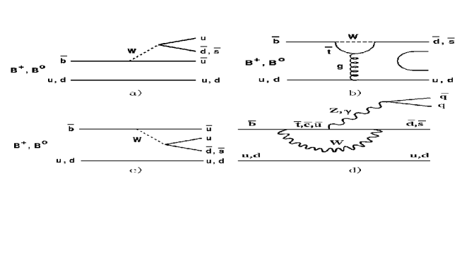
Figure 1: The dominant decay processes are expected to be a) external W-emission, b)gluonic Penguin, c) internal W-emission, d) external electroweak Penguin.

The CLEO II experiment [2] has accumulated $3.3\times 10^{6}\ B\bar{B}$ pairs. With typical efficiencies for two-body final states of $20-40\%$, and backgrounds of only a fraction of an event per million $B\bar{B}$ pairs we are sensitive to branching fractions as low as a few times $10^{-6}$, in some cases. Predictions for the dominant $T$ and $P$ amplitudes translate into branching fractions at a level of one to few times $10^{-5}$. We are therefore in a position to provide first experimental tests of theoretical predictions for absolute [3], as well as ratios of branching fractions [4].

Many authors have proposed to use charmless hadronic $B$ decays to probe the CKM sector of the standard model. For a recent review of this topic see for example Ref. [5]. An experimental test of the hierarchy of decay amplitudes presented above is crucial to assess the experimental and theoretical feasibility of probing the standard model in this manner.

2 Experimental Results

The Cornell Electron Storage Ring (CESR) is a symmetric $e^{+}e^{-}$ collider operating at a center of mass energy near the $\Upsilon$ resonances. The hadronic cross section for continuum production of u, d, s, or c quark anti-quark pairs is about a factor of 3 higher than that for $e^{+}e^{-}\to\Upsilon(4S)\to B\bar{B}$. This continuum production is the dominant background to the $B$ decays of interest here.

The CLEO II detector [2] boasts excellent charged and neutral particle detection. The momenta of charged particles is measured in a tracking system consisting of a 6-layer straw tube chamber,a 10-layer precision drift chamber, and a 51-layer main drift chamber, all operating inside a 1.5 T superconducting solenoid. The main drift chamber also provides a measurement of dE/dx used for particle identification. Photons are detected using 7800 CsI crystals, which are also inside the solenoid. The return yoke is instrumented at various depths with proportional counters to identify muons. CLEO II has accumulated a grand total of $3.3$ million $B\bar{B}$ pairs.

Table 1 lists the measured branching fractions and upper limits for charmless hadronic $B$ decays to $\pi\pi,\ K\pi,\ KK$ as well as final states containing an $\eta$ or $\eta^{{}^{\prime}}$. This is an update to a previously published analysis [6]. The main difference being a $30\%$ increase in data, and loosening of continuum background suppression cuts to increase the efficiency by $\approx 12\%$. Furthermore, we have extended the analysis to look for modes containing $\eta$ or $\eta^{{}^{\prime}}$.

Table 1: Summary of PRELIMINARY CLEO results for $B\to K\pi,\pi\pi,KK,h^{+}\eta,h^{+}\eta^{{}^{\prime}}$. The results for $K^{0}\pi^{0}$ and $\pi^{0}\pi^{0}$ are CLEO(1995) Results (PRD 53, 1039 (1996)). An update for these final states is still in progress.

Mode	Eff (%)	Yield	Signif	BR ($10^{-5}$)	UL ($10^{-5}$)
$K^{\pm}\pi^{\mp}$	44	$21.7_{-6.0}^{+6.8}$	5.6$\sigma$	$1.5^{+0.5+0.1}_{-0.4-0.1}\pm 0.1$
$K^{\pm}\pi^{0}$	37	$8.7_{-4.2}^{+5.3}$	2.7$\sigma$	$0.7\pm 0.4$	1.6
$K^{0}\pi^{\pm}$	12	$9.2_{-3.8}^{+4.3}$	3.2$\sigma$	$2.3^{+1.1+0.2}_{-1.0-0.2}\pm 0.2$	4.4
$K^{0}\pi^{0}$ *	7	$2.3^{+2.2}_{-1.5}$			4.0
$\pi^{\pm}\pi^{\mp}$	44	$10.0^{+6.8}_{-6.0}$	2.2$\sigma$	$0.7\pm 0.4$	1.5
$\pi^{\pm}\pi^{0}$	37	$11.3^{+6.3}_{-5.2}$	2.8$\sigma$	$0.9^{+0.6}_{-0.5}$	2.0
$\pi^{0}\pi^{0}$ *	26	$1.2^{+1.7}_{-0.9}$			0.9
$K^{\pm}K^{\mp}$	44	$0.0_{-0.0}^{+1.3}$	0.0$\sigma$		0.4
$K^{\pm}K^{0}$	12	$0.6_{-0.6}^{+3.8}$	0.2$\sigma$		2.1
$K^{0}\bar{K^{0}}$	5	0			1.7
$K^{+}\eta^{{}^{\prime}}$	5	$12.0\pm 3.7$	5.5$\sigma$	$7.8^{+2.7}_{-2.2}\pm 1.0$
$\pi^{+}\eta^{{}^{\prime}}$	5	$1.4^{+2.0}_{-1.0}$	2.0$\sigma$		4.4
$h^{+}\eta$	9	0			0.8
$h^{\pm}\pi^{\mp}$	44	$31.7^{+8.4}_{-7.3}$	7.8$\sigma$	$2.2^{+0.6}_{-0.5}$
$h^{\pm}\pi^{0}$	37	$20.0^{+6.8}_{-5.9}$	5.5$\sigma$	$1.6^{+0.6+0.3}_{-0.5-0.2}\pm 0.1$
$h^{\pm}{K^{0}}$	12	$9.8^{+4.5}_{-4.0}$	4.4$\sigma$	$2.4^{+1.1+0.2}_{-1.0-0.2}\pm 0.2$

In this paper we provide only a brief description of the analysis. Further details can be found in Refs. [6, 7]. Two kinematic variables, $\mathrm{M_{B}}=\sqrt{\mathrm{E^{2}_{beam}}-\mathrm{P^{2}_{B}}},\mathrm{\ and\ }\Delta\mathrm{E}=\mathrm{E}_{1}+\mathrm{E}_{2}-\mathrm{E_{beam}}$ are used to form a two dimensional signal plus sideband region. Using the beam energy in $M_{B}$ improves the mass resolution by an order of magnitude, resulting in $\sigma_{\mathrm{M_{B}}}\approx 2.6$MeV.

The main continuum background suppression is obtained by requiring $|\cos\theta_{sph}|<0.8$. The angle $\theta_{sph}$ here is the angle between the candidate axis and the sphericity axis of the rest of the event. Candidate $B$ daughters from continuum background tend to be the leading particles in two back to back 5 GeV “jets”. Background therefore peaks towards $\cos\theta_{sph}=\pm 1$. Signal is flat in $\cos\theta_{sph}$ as the two $B$’s are approximately at rest in the labframe, leading to uncorrelated directions for the decay products. This difference in “event shape” between $B\bar{B}$ signal and continuum background is exploited further using a Fisher Discriminant technique ($\cal F$) described in detail in Ref. [7]. The yield is determined using a maximum likelihood fit for the fraction of signal and background events out of the total number of events. As input to the fit $M_{B},\ \Delta E,\ {\cal F},\ \cos\theta_{B}$, and $dE/dx$ information are used. The angle $\theta_{B}$ is the $B$ decay angle with respect to the z-axis in the labframe. Decays of $\eta^{{}^{\prime}}$ are reconstructed in $\eta^{{}^{\prime}}\to\eta\pi^{+}\pi^{-}\to\gamma\gamma\pi^{+}\pi^{-}$. The search for $B^{+}\to h^{+}\eta$ includes $\eta\to\gamma\gamma$ as well as $\eta\to\pi^{+}\pi^{-}\pi^{0}$. The $\eta,\ \eta^{{}^{\prime}}$ mass is used as further input to the maximum likelihood fit where applicable. And $\cos\theta_{B}$ is used as part of $\cal F$ rather than in the fit in those cases.

Mass distributions for $B$ decays to $K^{+}\pi^{-},\ K^{0}h^{+},\ K^{+}\eta^{{}^{\prime}}$ and $h^{+}\pi^{0}$ are shown in Figure 2. Additional cuts are applied to suppress backgrounds in these plots. The curves are the PDF used in the fit normalized to the fit result times the efficiency of the additional cuts applied.

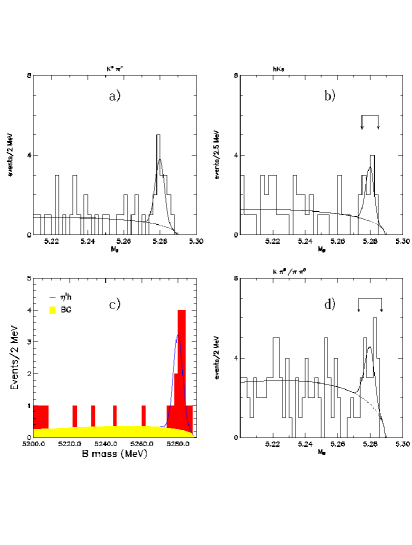
Figure 2: Mass distributions for $B$ decays to a)$K^{+}\pi^{-}$, b)$K^{0}h^{+}$, c)$K^{+}\eta^{{}^{\prime}}$ and d)$h^{+}\pi^{0}$. Projections from the fit are also shown.

3 Discussion of Results

3.1 $\Delta S=1$ Transitions

We have measured the branching fractions for exclusive $B$ decays to the final states $K^{+}\pi^{-},\ K^{0}\pi^{+}$ and $K^{+}\eta^{{}^{\prime}}$. All three of these are $\Delta S=1$ transitions.

It is very instructive to compare the square root of the three measured branching fractions with each other, as well as the diagrams that are expected to contribute. For simplicity we ignore diagrams that are expected to be suppressed by $O(\lambda^{2})$. For completeness, we have also listed the upper limits in $h^{+}\eta,\ K^{0}\pi^{0}$ and the central value from the fit in $K^{+}\pi^{0}$.

$$\begin{array}[]{ccccc}A_{K^{0}\pi^{+}}&=&(4.8^{+1.1}_{-1.0})\times 10^{-3}&&|P|\\ A_{K^{+}\pi^{-}}&=&(3.9^{+0.6}_{-0.5})\times 10^{-3}&&|T+P|\\ \sqrt{6}/3\times A_{K^{+}\eta^{{}^{\prime}}}&=&(7.2^{+1.5}_{-1.2})\times 10^{-3}&&{1\over 3}|T+3P+4P_{1}+(c_{u}+3c_{d})P_{EW}|\\ \sqrt{3}\times A_{K^{+}\eta}&<&4.9\times 10^{-3}&&|T+P_{1}+c_{u}P_{EW}|\\ \sqrt{2}\times A_{K^{0}\pi^{0}}&<&8.9\times 10^{-3}&&|P-(c_{u}-c_{d})P_{EW}|\\ \sqrt{2}\times A_{K^{+}\pi^{0}}&=&(3.7^{+1.1}_{-0.9})\times 10^{-3}&&|T+P+(c_{u}-c_{d})P_{EW}|\\ \end{array}$$ (2)

The amplitude $P_{1}$ enters due to $\eta_{1}-\eta_{8}$ mixing. It refers to the flavor singlet penguin diagram. We have followed Ref. [8] in our choice of mixing angle of $\phi=\sin^{-1}(1/3)\approx 20^{\circ}$. For this choice of $\phi$ there is no flavor octet contribution $P$ in $B^{+}\to K^{+}\eta$. Varying this angle within its known range [9] makes no difference to the general arguments presented here.

The branching fraction in $K^{0}\pi^{+}$ sets the scale by providing a direct measurement of the $P$ amplitude. Measured branching fractions and upper limits for all other $\Delta S=1$ transitions are consistent with being dominated by the measured $P$ amplitude. In particular, we see no need to invoke a $c\bar{c}$ or glueball component, nor anomalous coupling of two gluons to $\eta^{{}^{\prime}}$ in order to explain the relative size of these branching fractions [10].

Theoretical predictions of absolute branching fractions have large uncertainties due to factorization hypothesis and poorly known form factors. Keeping that in mind, theoretical predictions  [3, 11, 15]  of ${\cal B}(B^{+}\to\pi^{+}K^{0})\approx(1-2)\times 10^{-5}$ agree surprisingly well with our experimental result.

Let us look at Eq. (2) in some more detail. To $O(\lambda^{4})$, the only non-trivial weak phases in the CKM-matrix are those of $V_{ub}$ and $V_{td}$. The relative weak phase between $T$ and $P$ for $\Delta S=1$ transitions is thus the phase of $V_{ub}$. The ratio of ${\cal B}(B^{0}\to K^{+}\pi^{-})/{\cal B}(B^{+}\to K^{0}\pi^{+})$ may therefore provide constraints on the poorly known phase of $V_{ub}$ as was pointed out in Ref. [11].

The ratio of flavor singlet to flavor octet gluonic penguin diagrams $|P_{1}/P|$ is rather difficult to estimate theoretically. Neglecting $T$ and $P_{EW}$, we find that our current upper limit on ${\cal B}(B^{+}\to K^{+}\eta)$ is consistent with the naive expectation of $|P_{1}|<|P|$. This may provide a more stringent limit on $|P_{1}|$ as we increase our data set. Similarly, a significant discrepancy between the ratio of branching fractions for $K^{0}\pi^{+}/K^{+}\pi^{-}$ and $K^{0}\pi^{0}/K^{+}\pi^{0}$ may in the future provide a lower limit on $|$$P_{EW}$$|$. Construction of an amplitude quadrangle for these modes may in certain cases even provide information on the relative phases of these amplitudes.

3.2 $\Delta S=0$ Transitions

While we do see some excess of events above background in $\pi^{+}\pi^{-}$ and $\pi^{+}\pi^{0}$, the respective statistical significance of $2.2\sigma$ and $2.8\sigma$ is quite marginal. Both of these decay modes are expected to be dominated by simple external W-emission ($T$) diagrams. Factorization may therefore be less questionable here than in the $\Delta S=1$ transitions discussed above.

Using the CLEO measurement ${\cal B}(B^{0}\to\pi^{-}l^{+}\nu)=(2.0\pm 0.5\pm 0.3)\times 10^{-4}$  [12] we can use the factorization hypothesis, ISGW II, and the QCD factor $a_{1}=1.01\pm 0.02$ [13] to predict the branching fractions ${\cal B}(B^{0}\to\pi^{+}\pi^{-})=(1.3\pm 0.4)\times 10^{-5}$ and ${\cal B}(B^{+}\to\pi^{+}\pi^{0})=(0.7\pm 0.2)\times 10^{-5}$ respectively [14]. Uncertainties in the formfactor and factorization hypothesis are not reflected in the errors quoted here. Furthermore, contributions from anything other than the $T$diagram are neglected in this kind of comparison. Keeping this in mind, we conclude that the central value from the fit to the experimental data as shown in Table 1 compares well with these predictions.

We do not see any evidence for $B^{0}\to\pi^{0}\pi^{0}$ or $K^{0}\bar{K}^{0}$. The dominant contributions to these decays are due to ($C-P$), and $P$ respectively. The penguin diagrams in both cases are $b\to d$ penguins. Theoretical predictions for these modes range from less than $10^{-7}$ to few times $10^{-6}$[3, 15].

Finally, we see no evidence for $B^{0}\to K^{+}K^{-}$. This is not surprising as this decay can only proceed via $E$ or $PA$ diagrams. Theoretical predictions for this process are at the level of at most a few times $10^{-8}$[16].

We can therefore conclude that an overall consistent picture of charmless hadronic $B$ decays to two pseudoscalar mesons is starting to emerge. CLEO has measured the dominant $\Delta S=1$ transitions at levels consistent with theoretical predictions. No signals are found in any of the decay modes that are expected to be suppressed.

4 Acknowledgments

Many thanks to all the other people involved in the search for $B$ decays to two charmless pseudoscalar mesons at CLEO: Peter Gaidarev, Jim Alexander, Peter Kim, Andrei Gritsan, Jean Roy, and Jim Smith. Further thanks go to Lawrence Gibbons for information concerning the factorization test, and to Robert Fleischer, Karl Berkelman and Jim Smith for many useful discussions.

References

- [1] M. Gronau, O.F. Hernández, D. London, and J.L. Rosner, Phys. Rev. D 52, 6374 (1995); M. Gronau, O.F. Hernández, D. London, and J.L. Rosner, Phys. Rev. D 52, 6356 (1995).
- [2] Y.Kubota Nucl. Instrum. Methods A320, 66 (1992)
- [3] A.Deandrea et al.,Phys. Lett. B 318, 549 (1993), Phys. Lett. B 320, 170 (1994); L.-L.Chau,Phys. Rev. D 43, 2176 (1991), N.G.Deshpande and J.Trampetic Phys. Rev. D 41, 895 (1990); M.Bauer, B.Stech, M.Wirbel, Z. Phys. C 34, 103 (1987).
- [4] D. Zeppenfeld, Z. Phys. C 8, 77 (1981); M.J.Savage, M.B.Wise, Phys. Rev. D 39, 3346 (1989), Erratum: Phys. Rev. D 40, 3127 (1989); M.Gronau and D.London, Phys. Rev. Lett. 65, 3381 (1990); M. Gronau, O.F. Hernández, D. London, and J.L. Rosner, Phys. Rev. D 50, 4529 (1994);
- [5] R.Fleischer, Int.J.Mod.Phys.A12, 2459 (1997).
- [6] CLEO, Phys. Rev. D 53, 1039 (1996).
- [7] F.Würthwein, Ph.D., Cornell Jan. 1995; P.Gaidarev, Ph.D., Cornell 1997.
- [8] A.S. Dighe, M. Gronau, and J.L. Rosner, Phys. Lett. B 367, 357 (1996); Erratum: B377 325 (1996).
- [9] F.J. Gilman, R. Kaufman, Phys. Rev. D 36, 2761 (1987); 37 3348(E) (1988).
- [10] I.Halperin, A.Zhitnitsky, hep-ph/9704412; D.Atwood, A.Soni, hep-ph/9704357.
- [11] R.Fleischer, T.Mannel, hep-ph/9704423.
- [12] CLEO, Phys. Rev. Lett. 77, 5000 (1996).
- [13] A.J.Buras, Nucl. Phys. B 434, 606 (1995). Using the measured value (T.E.Browder hep-ph/9611373) makes no difference.
- [14] L.Gibbons, private communication.
- [15] M.Ciuchini, E.Franco, G.Martinelli, L.Silvestrini, hep-ph/9703353.
- [16] D.Du, L.Guo, D.Zhang predict (hep-ph/9706214) . Multiplying this by leads to .