B. Abbott
28
M. Abolins
25
B.S. Acharya
43
I. Adam
12
D.L. Adams
37
M. Adams
17
S. Ahn
14
H. Aihara
22
G.A. Alves
10
E. Amidi
29
N. Amos
24
E.W. Anderson
19
R. Astur
42
M.M. Baarmand
42
A. Baden
23
V. Balamurali
32
J. Balderston
16
B. Baldin
14
S. Banerjee
43
J. Bantly
5
J.F. Bartlett
14
K. Bazizi
39
A. Belyaev
26
S.B. Beri
34
I. Bertram
31
V.A. Bezzubov
35
P.C. Bhat
14
V. Bhatnagar
34
M. Bhattacharjee
13
N. Biswas
32
G. Blazey
30
S. Blessing
15
P. Bloom
7
A. Boehnlein
14
N.I. Bojko
35
F. Borcherding
14
J. Borders
39
C. Boswell
9
A. Brandt
14
R. Brock
25
A. Bross
14
D. Buchholz
31
V.S. Burtovoi
35
J.M. Butler
3
W. Carvalho
10
D. Casey
39
Z. Casilum
42
H. Castilla-Valdez
11
D. Chakraborty
42
S.-M. Chang
29
S.V. Chekulaev
35
L.-P. Chen
22
W. Chen
42
S. Choi
41
S. Chopra
24
B.C. Choudhary
9
J.H. Christenson
14
M. Chung
17
D. Claes
27
A.R. Clark
22
W.G. Cobau
23
J. Cochran
9
W.E. Cooper
14
C. Cretsinger
39
D. Cullen-Vidal
5
M.A.C. Cummings
16
D. Cutts
5
O.I. Dahl
22
K. Davis
2
K. De
44
K. Del Signore
24
M. Demarteau
14
D. Denisov
14
S.P. Denisov
35
H.T. Diehl
14
M. Diesburg
14
G. Di Loreto
25
P. Draper
44
Y. Ducros
40
L.V. Dudko
26
S.R. Dugad
43
D. Edmunds
25
J. Ellison
9
V.D. Elvira
42
R. Engelmann
42
S. Eno
23
G. Eppley
37
P. Ermolov
26
O.V. Eroshin
35
V.N. Evdokimov
35
T. Fahland
8
M. Fatyga
4
M.K. Fatyga
39
J. Featherly
4
S. Feher
14
D. Fein
2
T. Ferbel
39
G. Finocchiaro
42
H.E. Fisk
14
Y. Fisyak
7
E. Flattum
14
G.E. Forden
2
M. Fortner
30
K.C. Frame
25
S. Fuess
14
E. Gallas
44
A.N. Galyaev
35
P. Gartung
9
T.L. Geld
25
R.J. Genik II
25
K. Genser
14
C.E. Gerber
14
B. Gibbard
4
S. Glenn
7
B. Gobbi
31
M. Goforth
15
A. Goldschmidt
22
B. Gómez
1
G. Gómez
23
P.I. Goncharov
35
J.L. González Solís
11
H. Gordon
4
L.T. Goss
45
K. Gounder
9
A. Goussiou
42
N. Graf
4
P.D. Grannis
42
D.R. Green
14
J. Green
30
H. Greenlee
14
G. Grim
7
S. Grinstein
6
N. Grossman
14
P. Grudberg
22
S. Grünendahl
39
G. Guglielmo
33
J.A. Guida
2
J.M. Guida
5
A. Gupta
43
S.N. Gurzhiev
35
P. Gutierrez
33
Y.E. Gutnikov
35
N.J. Hadley
23
H. Haggerty
14
S. Hagopian
15
V. Hagopian
15
K.S. Hahn
39
R.E. Hall
8
S. Hansen
14
J.M. Hauptman
19
D. Hedin
30
A.P. Heinson
9
U. Heintz
14
R. Hernández-Montoya
11
T. Heuring
15
R. Hirosky
15
J.D. Hobbs
14
B. Hoeneisen
1,†
J.S. Hoftun
5
F. Hsieh
24
Ting Hu
42
Tong Hu
18
T. Huehn
9
A.S. Ito
14
E. James
2
J. Jaques
32
S.A. Jerger
25
R. Jesik
18
J.Z.-Y. Jiang
42
T. Joffe-Minor
31
K. Johns
2
M. Johnson
14
A. Jonckheere
14
M. Jones
16
H. Jöstlein
14
S.Y. Jun
31
C.K. Jung
42
S. Kahn
4
G. Kalbfleisch
33
J.S. Kang
20
R. Kehoe
32
M.L. Kelly
32
C.L. Kim
20
S.K. Kim
41
A. Klatchko
15
B. Klima
14
C. Klopfenstein
7
V.I. Klyukhin
35
V.I. Kochetkov
35
J.M. Kohli
34
D. Koltick
36
A.V. Kostritskiy
35
J. Kotcher
4
A.V. Kotwal
12
J. Kourlas
28
A.V. Kozelov
35
E.A. Kozlovski
35
J. Krane
27
M.R. Krishnaswamy
43
S. Krzywdzinski
14
S. Kunori
23
S. Lami
42
H. Lan
14,∗
R. Lander
7
F. Landry
25
G. Landsberg
14
B. Lauer
19
A. Leflat
26
H. Li
42
J. Li
44
Q.Z. Li-Demarteau
14
J.G.R. Lima
38
D. Lincoln
24
S.L. Linn
15
J. Linnemann
25
R. Lipton
14
Q. Liu
14,∗
Y.C. Liu
31
F. Lobkowicz
39
S.C. Loken
22
S. Lökös
42
L. Lueking
14
A.L. Lyon
23
A.K.A. Maciel
10
R.J. Madaras
22
R. Madden
15
L. Magaña-Mendoza
11
S. Mani
7
H.S. Mao
14,∗
R. Markeloff
30
L. Markosky
2
T. Marshall
18
M.I. Martin
14
K.M. Mauritz
19
B. May
31
A.A. Mayorov
35
R. McCarthy
42
J. McDonald
15
T. McKibben
17
J. McKinley
25
T. McMahon
33
H.L. Melanson
14
M. Merkin
26
K.W. Merritt
14
H. Miettinen
37
A. Mincer
28
J.M. de Miranda
10
C.S. Mishra
14
N. Mokhov
14
N.K. Mondal
43
H.E. Montgomery
14
P. Mooney
1
H. da Motta
10
C. Murphy
17
F. Nang
2
M. Narain
14
V.S. Narasimham
43
A. Narayanan
2
H.A. Neal
24
J.P. Negret
1
P. Nemethy
28
M. Nicola
10
D. Norman
45
L. Oesch
24
V. Oguri
38
E. Oltman
22
N. Oshima
14
D. Owen
25
P. Padley
37
M. Pang
19
A. Para
14
Y.M. Park
21
R. Partridge
5
N. Parua
43
M. Paterno
39
J. Perkins
44
M. Peters
16
R. Piegaia
6
H. Piekarz
15
Y. Pischalnikov
36
V.M. Podstavkov
35
B.G. Pope
25
H.B. Prosper
15
S. Protopopescu
4
J. Qian
24
P.Z. Quintas
14
R. Raja
14
S. Rajagopalan
4
O. Ramirez
17
L. Rasmussen
42
S. Reucroft
29
M. Rijssenbeek
42
T. Rockwell
25
N.A. Roe
22
P. Rubinov
31
R. Ruchti
32
J. Rutherfoord
2
A. Sánchez-Hernández
11
A. Santoro
10
L. Sawyer
44
R.D. Schamberger
42
H. Schellman
31
J. Sculli
28
E. Shabalina
26
C. Shaffer
15
H.C. Shankar
43
R.K. Shivpuri
13
M. Shupe
2
H. Singh
9
J.B. Singh
34
V. Sirotenko
30
W. Smart
14
A. Smith
2
R.P. Smith
14
R. Snihur
31
G.R. Snow
27
J. Snow
33
S. Snyder
4
J. Solomon
17
P.M. Sood
34
M. Sosebee
44
N. Sotnikova
26
M. Souza
10
A.L. Spadafora
22
R.W. Stephens
44
M.L. Stevenson
22
D. Stewart
24
D.A. Stoianova
35
D. Stoker
8
M. Strauss
33
K. Streets
28
M. Strovink
22
A. Sznajder
10
P. Tamburello
23
J. Tarazi
8
M. Tartaglia
14
T.L.T. Thomas
31
J. Thompson
23
T.G. Trippe
22
P.M. Tuts
12
N. Varelas
25
E.W. Varnes
22
D. Vititoe
2
A.A. Volkov
35
A.P. Vorobiev
35
H.D. Wahl
15
G. Wang
15
J. Warchol
32
G. Watts
5
M. Wayne
32
H. Weerts
25
A. White
44
J.T. White
45
J.A. Wightman
19
S. Willis
30
S.J. Wimpenny
9
J.V.D. Wirjawan
45
J. Womersley
14
E. Won
39
D.R. Wood
29
H. Xu
5
R. Yamada
14
P. Yamin
4
C. Yanagisawa
42
J. Yang
28
T. Yasuda
29
P. Yepes
37
C. Yoshikawa
16
S. Youssef
15
J. Yu
14
Y. Yu
41
Z.H. Zhu
39
D. Zieminska
18
A. Zieminski
18
E.G. Zverev
26
and A. Zylberstejn40
(DØ Collaboration)
1Universidad de los Andes, Bogotá, Colombia 2University of Arizona, Tucson, Arizona 85721 3Boston University, Boston, Massachusetts 02215 4Brookhaven National Laboratory, Upton, New York 11973 5Brown University, Providence, Rhode Island 02912 6Universidad de Buenos Aires, Buenos Aires, Argentina 7University of California, Davis, California 95616 8University of California, Irvine, California 92697 9University of California, Riverside, California 92521 10LAFEX, Centro Brasileiro de Pesquisas Físicas,
Rio de Janeiro, Brazil 11CINVESTAV, Mexico City, Mexico 12Columbia University, New York, New York 10027 13Delhi University, Delhi, India 110007 14Fermi National Accelerator Laboratory, Batavia,
Illinois 60510 15Florida State University, Tallahassee, Florida 32306 16University of Hawaii, Honolulu, Hawaii 96822 17University of Illinois at Chicago, Chicago,
Illinois 60607 18Indiana University, Bloomington, Indiana 47405 19Iowa State University, Ames, Iowa 50011 20Korea University, Seoul, Korea 21Kyungsung University, Pusan, Korea 22Lawrence Berkeley National Laboratory and University of
California, Berkeley, California 94720 23University of Maryland, College Park, Maryland 20742 24University of Michigan, Ann Arbor, Michigan 48109 25Michigan State University, East Lansing, Michigan 48824 26Moscow State University, Moscow, Russia 27University of Nebraska, Lincoln, Nebraska 68588 28New York University, New York, New York 10003 29Northeastern University, Boston, Massachusetts 02115 30Northern Illinois University, DeKalb, Illinois 60115 31Northwestern University, Evanston, Illinois 60208 32University of Notre Dame, Notre Dame, Indiana 46556 33University of Oklahoma, Norman, Oklahoma 73019 34University of Panjab, Chandigarh 16-00-14, India 35Institute for High Energy Physics, 142-284 Protvino,
Russia 36Purdue University, West Lafayette, Indiana 47907 37Rice University, Houston, Texas 77005 38Universidade Estadual do Rio de Janeiro, Brazil 39University of Rochester, Rochester, New York 14627 40CEA, DAPNIA/Service de Physique des Particules,
CE-SACLAY, Gif-sur-Yvette, France 41Seoul National University, Seoul, Korea 42State University of New York, Stony Brook,
New York 11794 43Tata Institute of Fundamental Research,
Colaba, Mumbai 400005, India 44University of Texas, Arlington, Texas 76019 45Texas A&M University, College Station, Texas 77843
Abstract
We present limits on anomalous and couplings from a
search for and production in collisions at
TeV. We use events recorded
with the DØ detector at the Fermilab Tevatron Collider during the
1992–1995 run. The data sample corresponds to an integrated luminosity of
pb-1. Assuming identical and coupling
parameters, the 95% CL limits on the –conserving couplings are
() and
(), for a form factor scale TeV. Limits based
on other assumptions are also presented.
pacs:
Submitted to Phys. Rev. Lett.
††preprint: Fermilab–Pub–97/136–E
The vector boson trilinear couplings predicted by the non-Abelian gauge
symmetry of the Standard Model (SM) can be measured directly in pair
production processes such as ,
, , and . Deviations from the SM
couplings would signal new physics. Studies of such effects have been
reported by the UA2 [3], CDF [4] and
DØ [5, 6, 7] collaborations. In this letter we report on the
measurement of couplings (where or ) using the
diboson production processes
and , where represents a
jet.
The Lorentz invariant Lagrangian which describes the and
interactions has fourteen independent coupling parameters [8],
seven describing the vertex and seven for the vertex.
Assuming electromagnetic gauge invariance and conservation, the
number of parameters is reduced to five: , ,
, and . In the SM at tree
level, the coupling parameters have the values , , . The SM cross sections for and production at the Tevatron,
at TeV, are 9.5 pb and 2.7 pb [9] respectively.
Non-SM values of the coupling parameters would result in an increase of
the production cross section, especially for large values of the
transverse momentum of the boson (). Since tree level unitarity
restricts the couplings to their SM values at asymptotically high
energies, each of the couplings must be modified by a form factor e.g.
, where
is the square of the invariant mass of the or system and
is the form-factor scale. We have used , and
TeV.
The analysis reported here uses events
recorded with the DØ detector during the 1992–1993 and 1993–1995
Fermilab Tevatron Collider runs at TeV, corresponding to
a total integrated luminosity of pb-1. The DØ detector and data collection system are described
elsewhere [10]. The basic elements of the trigger and
reconstruction algorithms for jets, electrons, and neutrinos are given in
Ref. [7]. The analysis of events from the 1992–1993
Tevatron Collider run ( pb-1) was reported
previously [6]. This letter focuses on the analysis of the
1993–1995 data set of pb-1 and gives the combined
results for both analyses. Further details are available in
Ref. [11].
The data sample was obtained with a trigger which required an isolated
electromagnetic (EM) calorimeter cluster with transverse energy
GeV and missing transverse energy
GeV. The offline event
selection required that the EM cluster have in the central
calorimeter or in an end calorimeter, where is the
pseudorapidity. Electrons were identified by requiring that the EM cluster
pass the shower profile and tracking information criteria, as described in
our earlier analysis [6]. The presence of a neutrino was inferred
from the , calculated from
the vector sum of the measured in each calorimeter tower. Jets were
reconstructed using a cone algorithm with radius . To remove spurious jets due
to detector effects, this analysis used the same quality cuts as were used
in Ref. [12]. Jets were required to be within .
The jet energies were corrected for effects of jet energy scale
calibration, out-of-cone showering, energy from the underlying
event [13], and energy loss due to out-of-cone gluon radiation.
The candidates were selected by searching for events containing an
isolated electron with high ( GeV), large
( GeV) and at least
two high jets ( GeV). The transverse mass of the electron
and neutrino system was required to be consistent with a decay ( GeV/c2, where is the azimuthal angle between the
electron and vector). The
invariant mass () of the two jet system (the largest invariant
mass if there were more than two jets with GeV in the event)
was required to be GeV/c2, as expected for a
or decay. Monte Carlo studies showed
that the dijet invariant mass resolution for signal events is 16
GeV/c2. The transverse momentum of the two gauge bosons was required to
be within GeV/c, as expected for
production.
There are two major sources of background to production: (i) jets with ; and (ii)
QCD multijet events where one of the jets is misidentified as an electron
and there is significant in
the event due to mismeasurement. Other backgrounds such as:
production with subsequent decay to followed by
; or production with
followed by ; , where
one electron is mismeasured or not identified; and with , are negligible.
The jets background was estimated using the vecbos [14] event generator, with , followed by
parton fragmentation using the herwig [15] package and a
detailed geant [16] based simulation of the detector.
Normalization of the jets background was determined by
comparing the number of events expected from the vecbos estimate to
the number of candidate events outside the dijet mass window, after the
multijet backgrounds had been subtracted. The systematic uncertainties in
this background are due to the normalization and to the jet energy scale
correction. The multijet background was estimated following the same
procedure used in our previous analysis [6]. The background sample,
which consisted of data events containing a jet satisfying the electron
trigger selection but failing the electron identification, was normalized
to the signal sample in the region
GeV where the actual
contribution is negligible. The number of background events was
then determined from this scaled background sample with the rest of the
selection criteria applied [11]. The backgrounds from
and other minor sources were
estimated using the isajet event generator [17] followed by
detector simulation. Table I summarizes the background estimates and the
total number of events seen. The number of observed events was consistent
with the background estimates which dominate the SM signal.
The trigger and offline electron identification efficiencies were
estimated using events. The trigger efficiency was
()% [5]. The electron identification efficiencies
were found to be ()% in the central calorimeter and
()% in the end calorimeters. We studied the efficiency for the jet cone size using the isajet and pythia [18] event generators followed by
detector simulation. The selection criteria were applied to these samples
and it was found that the efficiency was % for
GeV/c and that this decreased significantly for GeV/c due to
merging of the two jets into one. The efficiencies obtained from isajet were used to estimate the detection efficiencies of the
processes since they gave more conservative results.
The overall event selection efficiency was calculated using the
leading order event generator of Ref. [19] to generate four-momenta
for and processes as a function of the coupling parameter
values. A fast detector simulation was used to take into account the
detector resolutions and efficiencies described above. Higher order QCD
effects were approximated by a –factor [9] and a smearing of the transverse momentum of the
diboson system according to the experimentally determined spectrum
from the inclusive sample. The total selection
efficiencies for the detection of SM and events were estimated
to be [ (stat) (syst)]% and [ (stat) (syst)]%, respectively. The systematic uncertainty
(8%) includes: electron trigger and selection efficiencies (1%);
smearing and of the
diboson system (5%); difference between the isajet and pythia programs for efficiency parametrization (5%);
statistical uncertainty for efficiency parametrization
(2%); and jet energy scale (3%).
The expected signal for plus production with SM couplings is
events based on the total integrated luminosity of 96.0
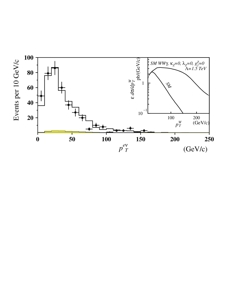
pb-1. Figure 1 shows the distributions
for candidate events from 1993–1995 data, total background estimate plus
SM expectations, and SM expectations for and production, after
all selection criteria have been applied. There is no clear difference
between the observed spectrum and that expected from
background plus SM and prediction.
Using the detection efficiencies for SM and production and the
background subtracted signal, and assuming the SM ratio of cross sections
for and production, we can set an upper limit at the 95% CL on
the cross section of pb.
Since we observed no excess of high events, large deviations
from the SM trilinear coupling values are excluded. Limits on the
anomalous coupling parameters were set by performing a binned likelihood
fit to the observed spectrum with the Monte Carlo signal
prediction plus the estimated background. Unequal width bins were used to
evenly distribute the observed events, especially those at the end of the
spectrum. In each bin for a given set of anomalous coupling
parameters, we calculated the probability for the sum of the background
estimate and Monte Carlo prediction to fluctuate to the observed
number of events. The limits on the anomalous coupling parameters are from
a combined likelihood fit to both data sets. The uncertainties in the
background estimates, efficiencies, integrated luminosity, and higher
order QCD corrections to the signal were convoluted with Gaussian
distributions into the likelihood function. Uncertainties common to both
analyses, e.g. theoretical uncertainties, were convoluted only once.
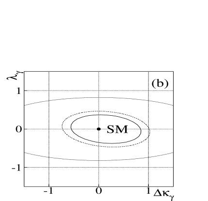
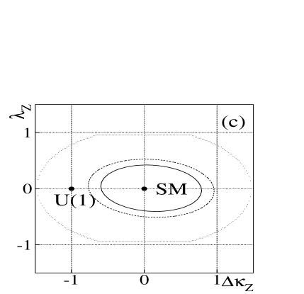
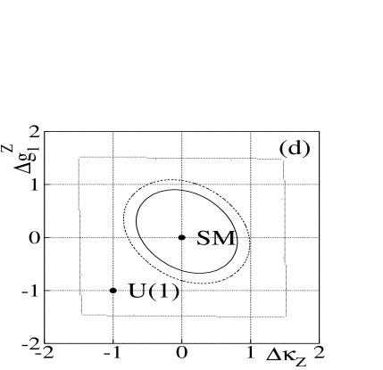
In Fig. 2, bounds on four pairs of coupling parameters
are shown using TeV. In each case all other couplings are
fixed to their SM values. The one- and two-degree-of-freedom 95% CL
contour limits (corresponding to likelihood function values 1.92 and 3.00
units below the maximum, respectively) are shown as the inner curves,
along with the S-matrix unitarity limits, shown as the outermost curves,
which are obtained by evaluating all (i.e. , , and )
processes. Figure 2(a) shows the contour limits when coupling parameters
for are assumed to be equal to those for . Figure 2(b)
shows contour limits assuming HISZ relations [20]. In Fig. 2(c) and
2(d) SM couplings are assumed and the coupling limits for
are shown.
When SM couplings are assumed, the U(1) point (,
, ) is excluded at the 99% CL. This is direct
evidence for the existence of the couplings.
Table II lists the 95% CL axis limits for three different values of
and four assumptions:
(i) ,
; (ii) HISZ relations; (iii) SM
couplings; and (iv) SM couplings. The results with the SM
assumption are unique to production since the
couplings are not accessible with production. The results
indicate that this analysis is more sensitive to couplings than to
ones as expected from the larger overall couplings for
than [8]. The dependence of the coupling parameters on
is clearly seen. Tighter limits are obtained when a larger value
for is used. When SM couplings are assumed, our limits on
and with TeV are
not tight enough to lie within the S-matrix unitarity limit.
In conclusion, we have presented limits on anomalous and
coupling parameters which are the most stringent to date. They are
significantly tighter than those from the analyses of the 1992–1993 data
set [4, 6], and significantly better on (but
comparable on ) to those measured using production with
the 1992–1995 data set [5].
We thank U. Baur for useful discussions and D. Zeppenfeld for providing us
with the and Monte Carlo generators. We thank the staffs at
Fermilab and collaborating institutions for their contributions to this
work, and acknowledge support from the Department of Energy and National
Science Foundation (U.S.A.), Commissariat à L’Energie Atomique
(France), State Committee for Science and Technology and Ministry for
Atomic Energy (Russia), CNPq (Brazil), Departments of Atomic Energy and
Science and Education (India), Colciencias (Colombia), CONACyT (Mexico),
Ministry of Education and KOSEF (Korea), CONICET and UBACyT (Argentina),
and the A.P. Sloan Foundation.
REFERENCES
[1]
Visitor from IHEP, Beijing, China.
[2]
Visitor from Universidad San Francisco de Quito, Quito, Ecuador.
[3] J. Alitti et al. (UA2 Collaboration), Phys.
Lett. B277, 194 (1992).
[4] F. Abe et al. (CDF Collaboration), Phys. Rev.
Lett. 74, 1936 (1995);
ibid., 74, 1941 (1995);
ibid., 75, 1017 (1995);
F. Abe et al. (CDF Collaboration), Fermilab–Pub–96/311–E,
to be published in Phys. Rev. Lett.
[5] S. Abachi et al. (DØ Collaboration),
Phys. Rev. Lett. 75, 1023 (1995);
ibid., 75, 1028 (1995);
ibid., 75, 1034 (1995);
ibid., 78, 3634 (1997);
ibid., 78, 3640 (1997).
[6] S. Abachi et al. (DØ Collaboration), Phys. Rev.
Lett. 77, 3303 (1996).
[7] S. Abachi et al. (DØ Collaboration),
Fermilab–Pub–97/088–E, hep–ex/9704004, submitted to Phys. Rev. D.
[8] K. Hagiwara, R.D. Peccei, D. Zeppenfeld and K. Hikasa,
Nucl. Phys. B282, 253 (1987).
[9] J. Ohnemus, Phys. Rev. D 44, 1403 (1991);
ibid., 44, 3477 (1991).
[10] S. Abachi et al. (DØ Collaboration), Nucl.
Instrum. Methods A338, 185 (1994).
[11] A. Sánchez-Hernández, Ph.D.
Dissertation, CINVESTAV,
Mexico City, Mexico (1997), unpublished.
[12] S. Abachi et al. (DØ Collaboration), Phys. Rev.
Lett. 75, 618 (1995).
[13] R. Kehoe (for the DØ Collaboration), preprint
Fermilab–Conf–96/284–E, to appear in Proc. 6th International Conf.
on Calorimetry in High Energy Physics, Frascati (1996).
[14] F.A. Berends et al., Nucl. Phys. B357,
32 (1991). We used version 3.0.
[15] G. Marchesini et al., Comput. Phys. Commun. 67, 465 (1992). We used version 5.7.
[16] F. Carminati et al., geant Users
Guide, CERN Program Library Long Writeup WS013 (1993), unpublished.
[17] F. Paige and S. Protopopescu, BNL Report BNL38034 (1986),
unpublished. We used version 7.22.
[18] T. Sjöstrand, Comput. Phys. Commun. 82, 74
(1994).
[19] K. Hagiwara, J. Woodside and D. Zeppenfeld, Phys. Rev. D
41, 2113 (1990); D. Zeppenfeld (private communication).
[20] K. Hagiwara, S. Ishihara, R. Szalapski and D. Zeppenfeld,
Phys. Rev. D 48, 2182 (1993); Phys. Lett. B 283, 353 (1992).
They parametrize the couplings in terms of the couplings:
, and .
TABLE I.: Summary of signal and backgrounds.
1992–1993
1993–1995
Luminosity
13.7 pb-1
82.3 pb-1
Backgrounds
2 jets
62.2
13.0
279.5
36.0
QCD Multijet
12.2
2.6
104.3
12.3
0.9
0.1
3.7
1.3
Total Background
75.3
13.3
387.5
38.1
Data
84
399
SM + prediction
3.2
0.6
17.5
3.0
TABLE II.: Axis limits at the 95% CL with various assumptions and three
different values.
Couplings / (TeV)
1.0
1.5
2.0
(i)
,
,
,
,
,
,
(ii)
(HISZ)
,
,
,
(HISZ)
,
,
,
(iii)
(SM )
,
,
,
(SM )
,
,
,
(SM )
,
,
,
(iv)
(SM )
,
,
(SM )
,
,
FIG. 1.:
distributions of the system for the 1993–1995 data set. The
points with error bars represent the data. The solid histogram is the
total background estimate plus the SM Monte Carlo predictions of and
production (shown as shaded histogram). The inset shows the predicted
, folded with the detection efficiencies, for SM
and couplings (lower curve), and for SM and
the indicated anomalous couplings (upper curve).
FIG. 2.:
Limits on –conserving anomalous couplings parameters: (a)
,
; (b) HISZ relations; (c) and
(d) SM couplings. The inner and middle curves represent 95% CL
one- and two-degree-of-freedom exclusion contours, respectively. The
outermost curves show S–matrix unitarity bounds. TeV is
used for all four cases. The SM prediction is ,
.