High Energy Muon Momentum Estimation from Multiple Coulomb Scattering in Dense Detectors

Abstract

A method is described for estimating muon track momentum from the distribution of hits along tracks in dense calorimeters due to multiple Coulomb scattering (MCS). The method requires only well-aligned conventional drift chambers or similar tracking devices and can be implemented with or without a magnetic field present. Neutrino experiments can use this technique to increase acceptance for large angle charged-current scattering events. Resolutions in a typical detector geometry vary from $\sim 10\%$ at $p=20$ GeV$/c$ to $\sim 50\%$ for $p=500$ GeV$/c$, if the number of hits on the track is sufficient.

1 Introduction

Neutrino detectors are commonly constructed as long dense calorimeters to maximize interaction rate. This geometry results in loss of acceptance for charged current $\nu_{\mu}$ interactions from muons that exit the sides before they reach the spectrometer that is typically immediately downstream of the calorimeter. In toroidally magnetized calorimeters, muons can exit before sufficient $BdL$ is accumulated to measure momentum, or they may leave a large fraction of their track length in the central hole of the toroid. Losses are greatest at high values of Bjorken scaling variable $x$ and inelasticity $y$.

Fortunately, these detectors are often instrumented with a large number of tracking chambers to determined the neutrino interaction vertex and muon scattering angle. Resolution on this angle can be dominated by multiple Coulomb scattering (MCS) up to TeV energies. Strong dependence of MCS error contribution on momentum and the large number of hits on a track in neutrino detectors permits a different momentum determination scheme. The procedure dates from the late thirties[1], has been used in many emulsion experiments[2], and is still used in balloon-borne cosmic ray experiments with a variety of tracking technologies[3]. It entails a straight line fit to a muon track that varies slope, intercept, and momentum such that the probability distribution for the observed pattern of hits is maximized. The MCS-based momentum estimation does not require a magnetic field and allows for a substantial recovery of the acceptance loss from exiting muons. Reasonable resolution can be obtained for muons with momenta up to several hundred GeV$/c$ using a straightforward track finding and fitting algorithm

The following sections describe the procedure in more detail and the results of calculations for a detector geometry consisting of $N$ identical tracking chambers with spatial resolution $\sigma_{0}$ separated from each other by a constant thickness $\Delta$ of material with radiation length $X_{0}$. The calculations are tested with a Geant[4] Monte Carlo simulation of the NuTeV neutrino experiment[5] at Fermi National Accelerator Laboratory. This experiment, chosen for its “typical” neutrino detector, is briefly described in Appendix A. It has parameter values of $N\leq 42$, $\sigma_{0}=0.05$ cm, $\Delta=42.4$ cm, and $X_{0}=3.45$ cm for the purposes of this paper. A forthcoming publication will provide results of application of the procedure to NuTeV data.

2 Tracks in a Dense Detector

2.1 $\chi^{2}$ Based Momentum Estimation

Consider fitting a small-angle muon track to a straight line in a dense calorimeter instrumented with many equally spaced tracking detectors (assumed to be drift chambers for the sake of discussion). This may be accomplished by minimizing a $\chi^{2}$ function that compares measured hit positions to a linear trajectory,

$$\chi^{2}=\left(\vec{y}-\theta_{0}\vec{z}_{1}-y_{0}\vec{z}_{0}\right){\bf V}^{-1}(p)\left(\vec{y}-\theta_{0}\vec{z}_{1}-y_{0}\vec{z}_{0}\right),$$ (1)

with respect to the slope $\theta_{0}$ and intercept $y_{0}$. Here, $\vec{y}$ and $\vec{z}_{1}$ are the $N$ measured $y,z$ points, and $\vec{z}_{0}$ is an $N$ dimensional vector with all of its elements equal to unity. The covariance matrix ${\bf V}(p)$ contains constant contributions from chamber resolution and momentum dependent terms from multiple Coulomb scattering (MCS):

$$V_{ij}=\sigma_{0}^{2}\delta_{ij}+S_{ij}(p),$$ (2)

where the scattering matrix element, usually attributed to Fermi[2], is

$$S_{ij}(p)=\sum_{k=1}^{\min(i,j)}\frac{\mu_{k}^{2}}{p_{k}^{2}}\left[\frac{\Delta_{k}^{2}}{3}+\frac{\Delta_{k}}{2}(z_{i}-z_{k}+z_{j}-z_{k})+(z_{i}-z_{k})(z_{j}-z_{k})\right].$$ (3)

In these expressions for the covariance matrix, $\sigma_{0}$ is the drift chamber resolution, $\Delta_{k}$ is the distance in $z$ between hits $k$ and $k-1$, $z_{i}$ is the distance from the track start to the $i^{th}$ hit, and $p_{k}$ is the momentum (in GeV$/c$) in the gap between hit $k$ and $k-1$; $\mu_{k}\simeq 0.015\sqrt{\Delta_{k}/X_{k}}$, with $X_{k}$ the radiation length, is a constant depending on the composition and thickness of the tracking medium. Parametrizations for $\mu_{k}$ are discussed further in Appendix C. The rms displacement in the length $\Delta_{k}$ of

$$\delta_{k}=\sqrt{\frac{1}{3}}\frac{\mu_{k}\Delta_{k}}{p_{k}},$$ (4)

is, for iron, given by

$$\delta_{k}\simeq 320\mbox{ }\mu\mbox{m }\frac{10\mbox{ GeV}/c}{p}\left(\frac{\Delta_{k}}{10\mbox{ cm}}\right)^{3/2}.$$ (5)

For 10 cm tracking chamber separation, this displacement is the same as a typical spatial resolution measurement of a drift chamber.

For constant chamber separation, one can set $\Delta_{k}=\Delta$, $\mu_{k}=\mu$ and incorporate energy loss effects in an approximate way to yield simplification:

$$S_{ij}(p) \simeq \frac{\mu^{2}\Delta^{2}\min\left(i,j\right)}{6p^{2}}\left\{\left[2\min\left(i,j\right)^{2}-3\left(i+j\right)\min\left(i,j\right)+6ij\right]\right.$$ (7)

$$+\frac{\Delta}{p}\left\langle\frac{dp}{dz}\right\rangle\left[\left(\min\left(i,j\right)+1\right)3\min\left(i,j\right)^{2}-4\left(i+j\right)\min\left(i,j\right)\right.$$

$$\left.\left.+i+j-\min\left(i,j\right)\right]\right\},$$

with $p$ the momentum at the start of the track. Many of the formulas presented here will assume the mean energy loss, $\left\langle\frac{dp}{dz}\right\rangle$, is zero for simplicity, although, as will be seen, incorporation of finite $\left\langle\frac{dp}{dz}\right\rangle$ can significantly improve momentum estimates from MCS.

If the calorimeter is instrumented with a sufficiently large number of drift chambers, it is possible to exploit MCS to estimate muon track momentum from the scatter of the hits along a muon track. This can be seen from the following intuitive argument: Best estimates for $\theta$ and $y_{0}$ follow from minimizing the $\chi^{2}:$

$$\theta_{0} = \frac{<yz_{1}>-<yz_{0}><z_{1}z_{0}>}{<z_{1}z_{1}>-<z_{1}z_{0}>^{2}},$$ (8)

$$y_{0} = \frac{<z_{1}z_{1}><yz_{0}>-<z_{1}z_{0}><yz_{1}>}{<z_{1}z_{1}>-<z_{1}z_{0}>^{2}}.$$ (9)

Bracketed quantities $<ab>$ are defined as

$$<ab>=\frac{\vec{a}{\bf V}^{-1}\vec{b}}{\vec{z}_{0}{\bf V}^{-1}\vec{z}_{0}};$$ (10)

they are unchanged by a re-scaling of the error matrix. In the MCS limit, it follows that $\theta_{0}$ and $y_{0}$ are independent of the momentum, implying that $\chi^{2}\propto p^{2}$. Now, suppose one adjusts $p$ until the $\chi^{2}$ probability density function attains its maximum. This occurs at $\chi^{2}\simeq N$, and if the fit is performed at some nominal momentum $p_{0}$ achieving $\chi^{2}=\chi_{0}^{2}$, then an estimate for the true momentum of the track is

$$p=p_{0}\sqrt{\frac{N}{\chi_{0}^{2}}.}$$ (11)

The MCS technique thus provides a momentum estimation method that does not require a magnetic field.

2.2 Likelihood Function Method

A more rigorous derivation begins with the observation that the joint probability function for $N$ correlated drift chamber hits can be written, assuming Gaussian errors, as

$$P(\vec{y};\theta_{0},y_{0},p)=\left(\frac{1}{2\pi}\right)^{N/2}\frac{1}{\sqrt{\det{\bf V}(p)}}\exp\left[-\frac{1}{2}\chi^{2}(\theta_{0},y_{0},p)\right],$$ (12)

with $\chi^{2}$ defined in equation 1. This can be converted to a $(-)$log likelihood function,

$${\cal L}=\frac{1}{2}\log(\det{\bf V}(p))+\frac{1}{2}\chi^{2}(\theta_{0},y_{0},p),$$ (13)

where terms independent of $y_{0}$, $\theta_{0}$, and $p$ have been dropped. Estimates for $y_{0}$, $\theta_{0}$, and $p$ follow from minimizing ${\cal L}$.

2.2.1 MCS dominated limit

In the multiple scattering limit, one can write ${\bf V}(p)\simeq\frac{p_{0}^{2}}{p^{2}}{\bf V}(p_{0})$, where $p_{0}$ is some nominal estimate of the momentum. From this, it follows that $\det{\bf V}(p)=\left(\frac{p_{0}^{2}}{p^{2}}\right)^{N}\det{\bf V}(p_{0})$ and $\chi^{2}(\theta_{0},y_{0},p)=\frac{p^{2}}{p_{0}^{2}}\chi^{2}(\theta_{0},y_{0},p_{0})$. In this limit, the log likelihood becomes, after dropping terms that are independent of $\theta_{0}$, $y_{0}$, and $p$

$${\cal L}\rightarrow-N\log p+\frac{p^{2}}{2p_{0}^{2}}\chi^{2}(\theta_{0},y_{0},p_{0}).$$ (14)

Minimizing with respect to the three fit parameters yields $\frac{\partial\chi^{2}}{\partial\theta_{0}}=\frac{\partial\chi^{2}}{\partial y_{0}}=0$, as before, and equation 11. One can also obtain an estimate of the uncertainty in $p$ from

$$\frac{1}{\sigma_{p}^{2}}=\frac{\partial^{2}{\cal L}}{\partial p^{2}}_{{\cal L=L}_{\max}}=\frac{2\chi^{2}(\theta_{0},y_{0},p_{0})}{p_{0}^{2}}.$$ (15)

If the fit is iterated until $p=p_{0}$ and the fit is reasonable so that $\chi^{2}\simeq N$, then

$$\frac{\sigma_{p}}{p}\rightarrow\frac{1}{\sqrt{2N}}\mbox{ (MCS limit)}.$$ (16)

2.2.2 Effects of Finite Spatial Resolution

In the more typical case where chamber resolution is not negligible, one must solve the coupled equations

$$\frac{\partial}{\partial y_{0}}\chi^{2}(\theta_{0},y_{0},p) = 0$$ (17)

$$\frac{\partial}{\partial\theta_{0}}\chi^{2}(\theta_{0},y_{0},p) = 0,$$ (18)

$$\frac{\partial}{\partial p}\left[\log(\det{\bf V}(p))+\chi^{2}(\theta_{0},y_{0},p)\right] = 0,$$ (19)

which can be accomplished via straightforward iterative methods by computer.

Insight into the intrinsic resolution of the MCS momentum error estimate can be gained by examining an approximate expression for the momentum resolution, derived in Appendix B:

$$\frac{\sigma_{p}}{p}=\left[2\sum_{n=1}^{N}\frac{\xi_{n}^{4}}{\left(\xi_{n}^{2}+\frac{p^{2}\sigma_{0}^{2}}{\mu^{2}\Delta^{2}}\right)^{2}}\right]^{-1/2},$$ (20)

where $\xi_{n}^{2}$ are the eigenvalues of the dimensionless scattering matrix ${\bf\tilde{S}}=\frac{p^{2}}{\mu^{2}\Delta^{2}}{\bf S}(p)$. For the geometry considered here, and ignoring energy loss, the relative momentum error is seen to be a universal function of the number of chambers $n$ and the ratio $p^{2}/p_{MCS}^{2},$

$$\frac{\sigma_{p}}{p}=F(n,p^{2}/p_{MCS}^{2}),$$ (21)

where

$$p_{MCS}=\frac{\mu\Delta}{\sigma_{0}},$$ (22)

defines a characteristic momentum scale (approximately $73$ GeV for the NuTeV detector). Figure 1 shows plots of $F(n,x)$ vs $n$ for different values of $x=p^{2}/p_{MCS}^{2}$. About 7 chambers are required to measure $p_{MCS}$ to $50\%$ fractional momentum error and 25 chambers to measure $10\times p_{MCS}$ to $50\%$. For a given number of chambers $n$ used on a track fit, one can define a critical value $x_{crit}(n)$, such that $\sigma_{p}/p\leq 50\%$ for $x\leq x_{crit}(n)$. Figure 2 shows a plot of $x_{crit}(n)$ vs $n$. For a given detector geometry, $x_{crit}(n)$ can be converted to $p_{crit}(n)$, the largest momentum that can be estimated from MCS scattering alone to $50\%$ resolution. Figure 3 shows a plot of $p_{crit}(n)$ vs $n$ for the NuTeV detector. Momentum values of to 300 GeV can be estimated using 21 chambers in the detector, and up to 1 TeV using all 42 chambers.

The MCS limit is $p^{2}/p_{MCS}^{2}\ll\xi_{n}^{2}$ for all $n$, in which case Eq. 16 is recovered. If intrinsic chamber resolution dominates, MCS-based momentum estimates will then provide resolutions that behave as

$$\frac{\sigma_{p}}{p}\rightarrow\sqrt{\frac{1}{2N}}\left(\frac{p}{p_{MCS}}\right)^{2}\mbox{ (resolution limit),}.$$ (23)

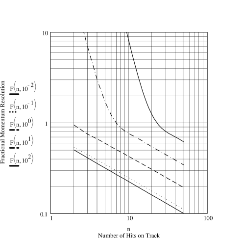
Figure 1: Universal resolution function $F(n,x)$ for MCS determination of momentum. The curves represent different values of $x=\frac{p\sigma_{0}}{\mu\Delta}$ which are $x=0.01$ (solid-lower), $x=0.1$ (dots), $x=1$ (dashed), $x=10$ (dot-dashed), and $x=100$ (solid-top).

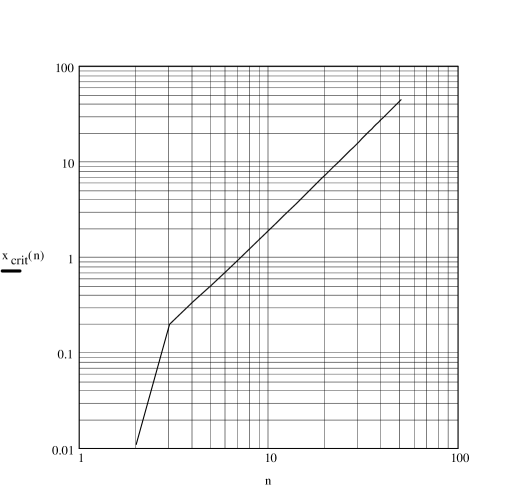
Figure 2: Critical value of $x=\frac{p\sigma_{0}}{\mu\Delta}$ as a function of number of drift chamber hits. For this value of $x$, the fractional momentum resolution will be 50%.

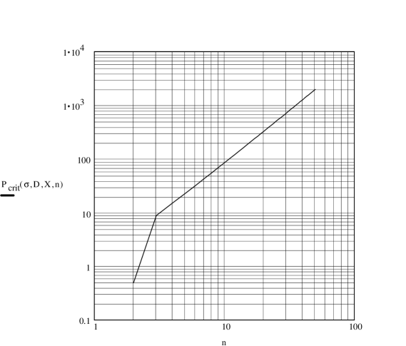
Figure 3: Value of critical momentum $P_{crit}$, above which the fractional momentum resolution will exceed 50% for a given number of drift chambers $n$. This plot assumes the NuTeV detector geometry, with $\sigma_{0}=0.05$ cm, $\Delta=42.4$ cm and 12.2 radiation lengths of material between each tracking chamber.

2.3 Tracking in a Magnetic Field

The much more straightforward way to determine momentum is via track displacement in a magnetic field. It is possible to combine the curvature measurement with the MCS momentum technique to improve the overall momentum estimation.

For simplicity, the analysis will be restricted to a geometry of evenly spaced tracking chambers immersed in a uniform magnetic field oriented at right angles to the track propagation. It is further assumed that the magnet $p_{T}$ kick is much less that the momentum of the track being analyzed. In this case there is no dependence of the covariance matrix on fit parameters other than momentum, and the variance matrix for the fitted momentum takes the form

$${\bf E}_{pp}^{-1}={\bf\Psi}^{-1}+\frac{1}{\sigma_{p}^{2}}\left(\begin{array}[]{lll}0&0&0\\ 0&0&0\\ 0&0&1\end{array}\right),$$ (24)

where $\sigma_{p}^{2}$ is given Eq. 20 and ${\bf\Psi}$ is the conventional spectrometer error matrix, with

$$\Psi_{11}^{-1} = \vec{z}_{0}{\bf V}^{-1}(p)\vec{z}_{0},$$ (25)

$$\Psi_{12}^{-1} = \vec{z}_{1}{\bf V}^{-1}(p)\vec{z}_{0},$$ (26)

$$\Psi_{22}^{-1} = \vec{z}_{1}{\bf V}^{-1}(p)\vec{z}_{1},$$ (27)

$$\Psi_{13}^{-1} = -\frac{k}{2p^{2}}\vec{z}_{0}{\bf V}^{-1}(p)\vec{z}_{2},$$ (28)

$$\Psi_{23}^{-1} = -\frac{k}{2p^{2}}\vec{z}_{1}{\bf V}^{-1}(p)\vec{z}_{2},$$ (29)

$$\Psi_{33}^{-1} = \frac{k^{2}}{4p^{4}}\vec{z}_{2}{\bf V}^{-1}(p)\vec{z}_{2},$$ (30)

Here,

$$\vec{z}_{0} = \left(1,1,1,...,1\right),$$ (31)

$$\vec{z}_{1} = \left(z_{1},z_{2},z_{3},...,z_{N}\right),$$ (32)

$$\vec{z}_{2} = \left(z_{1}^{2},z_{2}^{2},z_{3}^{2},...,z_{N}^{2}\right),$$ (33)

and $k=0.003B$, with $B$ the magnetic field in Tesla assuming all spatial coordinates are in cm.

In some detectors, such as NuTeV, the spectrometer follows the calorimeter. Spectrometer momentum determination and MCS-based calorimeter determination are then independent and can be averaged.

3 Results from Calculations

3.1 Tracking in Unmagnetized Calorimeter

Figures 4, 5, and 6 show results for the estimated fractional momentum error $\delta_{P}=(\sigma_{p}/p)$ calculated for the NuTeV detector geometry from Eq. 20 as a function of various parameters appearing in Eq. 20.

Figure 4 shows the dependence of fractional resolution on momentum for various numbers of drift chambers. Momentum dependence is present for all momenta and all numbers of chambers, indicating that the MCS resolution limit of $\sigma_{p}/p=1/\sqrt{2N}$ is not reached until lower momentum.

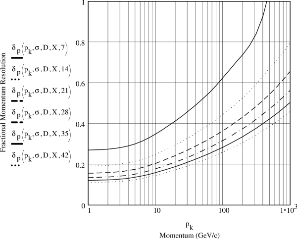
Figure 4: Momentum dependence of fractional momentum resolution for different numbers of chambers used in the fit. The curves correspond to 7 chambers (upper-solid), 14 chambers (upper-dotted), 21 chambers (dashed), 28 chambers (dot-dashed), 35 chambers (lower-solid), and the maximum possible 42 chambers (lower-dotted). This plot assumes the NuTeV detector geometry, with $\sigma_{0}=0.05$ cm, $\Delta=42.4$ cm, and 12.2 radiation lengths of material between each tracking chamber.

Figure 5 shows the dependence of $\sigma_{p}/p$ on the number of drift chamber hits. While the $1/\sqrt{2N}$ limit is not reached, the resolution does scale as $A/\sqrt{2N}$, with $A$ increasing with momentum.

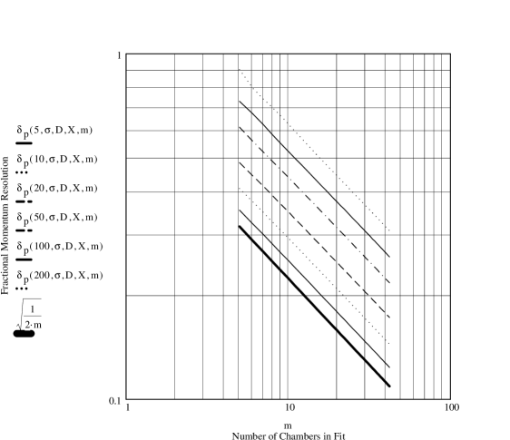
Figure 5: Dependence on number of drift chamber hits of fractional momentum resolution for different muon momenta. The dark solid curve represents the MCS limit. The other curves correspond to $p=5$ GeV$/c$ (lower-lighter solid), $p=10$ GeV$/c$ (lower-dotted), $p=20$ GeV$/c$ (dashed), $p=50$ GeV$/c$ (dot-dashed), $p=100$ GeV$/c$ (upper-solid), and $p=200$ GeV$/c$ (upper-dotted). This plot assumes the NuTeV detector geometry, with $\sigma_{0}=0.05$ cm, $\Delta=42.4$ cm, and 12.2 radiation lengths of material between each tracking chamber.

Figure 6 shows the dependence on chamber resolution. Effects are sizable, indicating that a careful assessment of the intrinsic chamber resolution is necessary.

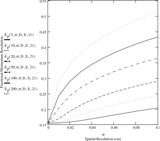
Figure 6: Spatial resolution dependence of fractional momentum resolution for different muon momenta assumes 21 drift chamber hits in the NuTeV geometry. The curves correspond to $p=5$ GeV$/c$ (lower-solid), $p=10$ GeV$/c$ (lower-dotted), $p=20$ GeV$/c$ (dashed), $p=50$ GeV$/c$ (dot-dashed), $p=100$ GeV$/c$ (upper-solid), and $p=200$ GeV$/c$ (upper-dotted). This plot otherwise assumes the NuTeV detector geometry, with $\Delta=42.4$ cm, and 12.2 radiation lengths of material between each tracking chamber.

3.2 Tracking in Magnetized Calorimeter

Figure 7, 8, and 9 show the dependence of fractional momentum resolution in a magnetized calorimeter as a function of muon momentum, magnetic field, and number of chambers respectively. Also shown is the resolution estimate for a conventional momentum fit that incorporates MCS effects into the error matrix, but uses only the track curvature, not the pattern of scatter in the hits, to estimate momentum. The three plots assume a geometry with 0.05 cm resolution drift chambers separated by 10 radiation lengths of material. Figures 7 and 9 assume a magnetic field of 1 T, Figs. 8 and 9 assume a muon momentum of 50 GeV, and Figs. 8 and 9 assume 20 chambers used in the fit.

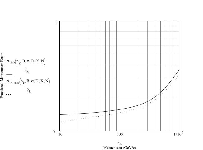
Figure 7: Dependence of fractional momentum resolution on muon momentum assuming twenty 0.05 cm resolution drift chamber hits spaced by 10 radiation lengths of iron. The top (solid) curve assumes a conventional spectrometer fit, while the lower (dotted) curve incorporates information from MCS into the fit.

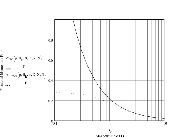
Figure 8: Dependence of fractional momentum resolution on magnetic field assuming twenty 0.05 cmm resolution drift chamber hits spaced by 10 radiation lengths of iron. The top (solid) curve assumes a conventional spectrometer fit, while the lower (dotted) curve incorporates information from MCS into the fit.

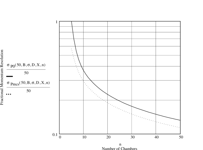
Figure 9: Dependence of fractional momentum resolution on number of drift chamber hits for 50 GeV muon momentum and 0.05 cm resolution drift chambers spaced by 10 radiation lengths of iron. The top (solid) curve assumes a conventional spectrometer fit, while the lower (dotted) curve incorporates information from MCS into the fit.

Figure 10 shows the combined momentum resolution that can be achieved from the spectrometer and a varying number of calorimeter chambers used in the NuTeV experiment. The spectrometer alone provides a resolution of $\varepsilon_{S}=10\%$.

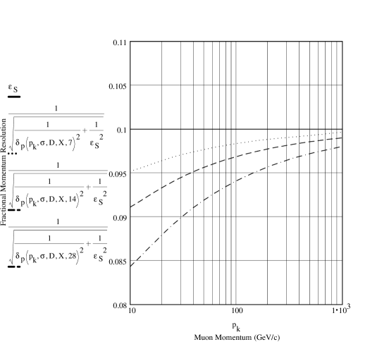
Figure 10: Dependence of fractional momentum resolution on muon momentum for different number of chambers used in the MCS determination in a momentum estimate that combines the MCS estimate with a 10% spectrometer measurement, $\varepsilon_{S}$, in the NuTeV geometry ($\sigma_{0}=0.05$ cm, $\Delta=42.4$ cm, and 12.2 radiation lengths of material between each tracking chamber). The curves correspond to 28 chambers (dot-dashed), 14 chambers (dashed), and 7 chambers (dotted). The solid horizontal line at 0.1 represents the spectrometer-only resolution.

4 Results of Monte Carlo Simulation

The formulas developed in the previous section have been tested using a Geant simulation of the NuTeV detector (see Appendix A) using track finding and fitting algorithms described in Appendix D. This section presents results only for tracking in the unmagnetized NuTeV calorimeter..

Figures 11 and 12 show distributions of fitted values of $1/p$ as a function of track momentum using all 42 chambers in the NuTeV detector. Results are presented for momentum determination using only a single view in the drift chamber, and for fits that combine both views. Table 1 summarizes momentum dependence of reconstructed momentum, fractional resolution, and tracking efficiency.

Figure 11: Distributions of $1/p$ (in (GeV$/c$)^-1) estimated from MCS technique for 20 GeV$/c$, 50 GeV$/c$, 100 GeV$/c$, and 200 GeV$/c$ muons passing through 42 drift chambers in a Geant simulation of the NuTeV neutrino detector. Only one of two drift chamber views is used in the fitting. The histograms are for, from right to left, 20 GeV$/c$ (solid), 50 GeV$/c$ (dashed), 100 GeV$/c$ (dotted), and 200 GeV$/c$ (dot-dashed) muons, respectively. The curves superimposed on the histograms represent simple Gaussian fits.

Figure 12: Distributions of $1/p$ (in (GeV$/c$)^-1) estimated from MCS technique for 20 GeV$/c$, 50 GeV$/c$, 100 GeV$/c$, and 200 GeV$/c$ muons passing through 42 drift chambers in a Geant simulation of the NuTeV neutrino detector. Both drift chamber views are used in the fitting. The histograms are for, from right to left, 20 GeV$/c$ (solid), 50 GeV$/c$ (dashed), 100 GeV$/c$ (dotted), and 200 GeV$/c$ (dot-dashed) muons, respectively. The curves superimposed on the histograms represent simple Gaussian fits.

${\bf p}_{in}$ (GeV$/c$)	20	50	100	200
${\bf p}_{rec}^{\mbox{1 view}}$(GeV$/c$)	20.6	46.0	93.4	194.0
${\bf p}_{rec}^{\mbox{2 views}}$(GeV$/c$)	20.8	46.5	94.0	195.0
${\bf\sigma/p}^{\mbox{1 view}}$	0.078	0.21	0.30	0.42
${\bf\sigma/p}^{\mbox{1 view}}$(pred)	0.17	0.22	0.26	0.31
${\bf\sigma/p}^{\mbox{2 views}}$	0.065	0.15	0.21	0.30
${\bf\sigma/p}^{\mbox{2 views}}$(pred)	0.12	0.15	0.18	0.22
${\bf\epsilon}_{p}^{\mbox{1 view}}{\bf(\%)}$	99	99	99	96
${\bf\epsilon}_{p}^{\mbox{2 views}}{\bf(\%)}$	99	99	99	93

Table 1: Momentum dependence of MCS momentum estimate from a Geant simulation of the NuTeV calorimeter. Results for reconstructed momentum ($p_{rec}$), resolution ($\sigma_{p}/p$), and reconstruction efficiency ($\epsilon_{p}$) are given assuming that either one or two views of drift chamber hits are used. The Monte Carlo sample contained $10^{4}$ events, so statistical errors are of order 1%.

Figures 13 and 14 show distributions of fitted values of $1/p$ as a function of the number of drift chambers used for a track momentum of 50 GeV$/c$. Results are presented for momentum determination using only a single view in the drift chamber, and for fits that combine both views. Table 2 summarizes chamber number dependence of fractional resolution and tracking efficiency.

Figure 13: Distributions of $1/p$ (in (GeV$/c$)^-1) estimated from MCS technique for 50 GeV$/c$ muons passing through different numbers of drift chambers in a Geant simulation of the NuTeV neutrino detector. Only one of two drift chamber views is used in the fitting. The plots are for, clockwise from top-left, 7 chambers, 14 chambers, 42 chambers, and 28 chambers used in the fit. The superimposed curves represent simple Gaussian fits.

Figure 14: Distributions of $1/p$ (in (GeV$/c$)^-1) estimated from MCS technique for 50 GeV$/c$ muons passing through different numbers of drift chambers in a Geant simulation of the NuTeV neutrino detector. Both drift chamber views are used in the fitting. The plots are for, clockwise from top-left, 7 chambers, 14 chambers, 42 chambers, and 28 chambers used in the fit. The curves superimposed on the histograms represent simple Gaussian fits.

${\bf N}$(chambers)	7	14	28	42
${\bf\sigma/p}^{\mbox{1 view}}$	0.56	0.49	0.30	0.20
${\bf\sigma/p}^{\mbox{1 view}}$(pred)	0.52	0.37	0.27	0.22
${\bf\sigma/p}^{\mbox{2 views}}$	0.44	0.35	0.22	0.16
$\sigma/p^{\mbox{2 views}}$(pred)	0.37	0.26	0.19	0.15
${\bf\varepsilon}^{\mbox{1 view}}{\bf(\%)}$	65	91	99	97
${\bf\varepsilon}^{\mbox{2 views}}{\bf(\%)}$	32	82	99	95

Table 2: Dependence of resolution, ($\sigma_{p}\over{p}$) and reconstruction efficiency ($\epsilon$) on number of chambers used in the fit for 50 GeV$/c$ input muons. Resulted are presented for fits using one or both views of the drift chamber. The Monte Carlo sample contained $10^{4}$ events, so statistical errors are of order 1%.

Agreement between observed resolution from the full reconstruction and Eq. 20 is satisfactory at 50 and 100 GeV$/c$. At 20 GeV$/c$, the observed resolution is considerably better than the prediction. Energy loss in the target is a significant fraction of the total muon energy in this case. The fitting procedure incorporates energy loss effects. Their inclusion introduces a second source of correlation between longitudinal chamber position and momentum that evidently enhances the resolution. Resolution at 200 GeV$/c$ is about $30\%$ worse in the Monte Carlo than predicted. The source for this disagreement is not fully understood, although it may be related to the significant tail that occurs on the high momentum side for fits to very high energy muons tracks. There are also small biases evident in the momentum reconstruction that, while much less than the momentum resolution, are not yet understood. For 50 GeV$/c$ muons, the resolution is observed to scale with the number of chambers as $1/\sqrt{N}$, in agreement with the prediction. The expected $\sqrt{1/2}$ improvement in resolution when combing the independent $x$ and $y$ views is also observed.

5 Systematic Errors

A proper survey of systematic errors requires treatment of real data, which will be presented in a forthcoming publication. A few obvious sources are commented upon here.

The theory of multiple Coulomb scattering is well-established[6, 7, 8]. The critical parameter that enters into fitting is $\mu_{k}$, which represents the effective rms of a Gaussian approximation to the distribution of the projected scattering angle. As discussed in Appendix C, different estimates for $\mu_{k}$ agree to within $\sim 2\%$ using simple parametrizations. It seems likely that this error could be reduced to negligible levels if a careful application of the Moliere theory is applied to a single material.

Any drift chamber misalignment will produce a bias in the MCS fitting procedure that produces a fitted momentum estimate that is systematically lower than the true value. Misplaced chambers will effectively introduce extra scatter between hits on a track. The only way the fitting routine can account for the extra scatter is to lower the momentum, thus increasing the contribution of MCS to ${\bf V}(p)$. If the misalignment is random, then the MCS fit will return relatively poor (high) values of the likelihood function. However, a correlated mis-alignment can mimic the effects of MCS fairly well. It is thus critical to have an accurate tracking chamber alignment.

Spurious hits not directly associated with the muon track from chamber noise or multiple-pulsing of electronics will also produce undesirable scatter that will bias momentum fits towards too low values. Electromagnetic shower particles produced by high energy particles in dense calorimeters will produce similar effects. It is thus important to use only hits from “quiet” intervals of the muon track where there is no possible ambiguity.

As is evident in Fig. 6 the resolution on the MCS fit is a fairly strong function of the chamber resolution $\sigma_{0}$. The MCS momentum estimate will also be biased by incorrect $\sigma_{0}$ values in a positively correlated way, i.e., the fit will return too high values of momentum to reduce the MCS error contribution if $\sigma_{0}$ is input at a value larger than its true value.

6 Conclusions

It has been demonstrated that momentum estimates based on multiple Coulomb scattering can be extended to work for very high energy muons in dense calorimeters instrumented with a sufficient number of typical drift chamber tracking detectors. Using the MCS technique could allow high energy neutrino experiments such as NuTeV at Fermilab to increase their acceptance for low energy, wide angle muons that exit their detector before a spectrometer momentum measurement is possible. Other possible applications exist in large detectors being assembled for long baseline neutrino oscillation searches, such as MINOS[14] at Fermilab.

Appendix A The NuTeV Detector

The NuTeV experiment will be used to provide specific examples of MCS momentum determination using analytic calculations and a detailed Monte Carlo simulation. NuTeV employs the Fermilab Lab E neutrino detector[11, 12] in a newly constructed high intensity sign-selected neutrino beam[13]. The experiment is currently taking data with the primary goal of measuring the weak mixing angle $\sin^{2}\theta_{W}\equiv 1-M_{W}^{2}/M_{Z}^{2}$ to a factor of 2-3 times the precision achieved in previous neutrino experiments. NuTeV will also make improved measurements of nucleon structure functions and will perform high sensitivity searches for processes not predicted by the Standard Model of electroweak physics.

The detector consists of a 690 ton iron target-calorimeter followed by an iron-core toroid spectrometer. The target-calorimeter is a 3 m$\times$3 m$\times$18 m volume centered with its long side parallel to the neutrino beam. Hadron energy measurement, longitudinal event vertex determination, and event triggering and timing are performing using eighty-four 3 m$\times$3 m $\times$2.5 cm liquid scintillation counters read out through wavelength-shifter bars to phototubes on each of the four corners of the counter. The scintillation counters are separated by 10 cm of steel, and provide a sampling-dominated hadronic energy resolution of $\sigma_{E}/E=0.9/\sqrt{E}+0.3/E$.

Transverse event vertex position and muon track angle in charged current events are measured in the target-calorimeter using up to forty-two 3m$\times$3m drift chambers which are spaced every 20 cm of steel. The drift chambers consist of two orthogonal planes, each containing twenty-four 12.7 cm wide cells. Each cell has two sense wires, permitting local left-right position ambiguity resolution. The chambers use a mixture of $50\%$ argon- $50\%$ ethane that produces a uniform 50 $\mu$m/ns drift velocity. Both sense wires of each cell are connected through shaping pre-amplifiers to multi-hit TDC’s; the TDC’s have 4 ns time buckets and can buffer up to 32 hits. When constructed and initially tested in the early eighties, the drift chamber resolution was measured to be 225 $\mu$m; the current resolution is estimated for studies in this paper to be $\sigma_{0}\simeq 500$ $\mu$m. Counting support structure, scintillation oil and other passive detector components, the drift chambers are separated by $42.4$ cm, corresponding to $12.2$ radiation lengths.

The toroid spectrometer the follows the calorimeter provides a $10\%$ MCS momentum resolution for muons from $5-500$ GeV$/c$.

NuTeV detector response is simulated using a Geant-based package[4] that produces output in the same form as the on-line data acquisition system. Multiple scattering is simulated using the default Moliere scattering option of Geant. Muon energy loss in iron is simulated using the Landau fluctuation process for restricted energy loss. Important contributions from catastrophic energy loss from muon bremsstrahlung and $e^{+}e^{-}$ pair emission are carefully modelled by lowering Geant photon and electron energy tracking cuts to 0.1 and 1.0 MeV, respectively.

Appendix B Derivation of MCS Momentum Resolution

If one ignores energy loss effects, the track error matrix can be expressed as

$${\bf V}(p) = \sigma^{2}{\bf I}+\frac{p_{0}^{2}}{p^{2}}{\bf S}(p_{0}^{2})$$

$$= {\bf V}(p_{0})+\left(\frac{p_{0}^{2}}{p^{2}}-1\right){\bf S}(p_{0}).$$

If

$${\bf V}(p_{0})\left|n\right\rangle=\lambda_{n}^{2}\left|n\right\rangle,$$ (35)

i.e., $\left\{\lambda_{n}^{2}\right\}$ are the eigenvalues of ${\bf V}(p_{0})$, then

$${\bf S}(p_{0})\left|n\right\rangle=\left(\lambda_{n}^{2}-\sigma^{2}\right)\left|n\right\rangle,$$ (36)

and thus,

$${\bf V}(p)\left|n\right\rangle=\left[\frac{p_{0}^{2}}{p^{2}}\left(\lambda_{n}^{2}-\sigma^{2}\right)+\sigma^{2}\right]\left|n\right\rangle,$$ (37)

so that

$$\log(\det{\bf V}(p))=\sum_{n}\log\left[\frac{p_{0}^{2}}{p^{2}}\left(\lambda_{n}^{2}-\sigma^{2}\right)+\sigma^{2}\right].$$ (38)

Letting $p=p_{0}+\delta_{p}:$

$$\log(\det{\bf V}(p)) \simeq \sum_{n}\log\left(\lambda_{n}^{2}\right)-\frac{2\left(\lambda_{n}^{2}-\sigma^{2}\right)}{\lambda_{n}^{2}}\left(\frac{\delta_{p}}{p_{0}}\right)$$

$$+\frac{\left(\lambda_{n}^{2}-\sigma^{2}\right)\left(\lambda_{n}^{2}+2\sigma^{2}\right)}{\lambda_{n}^{4}}\left(\frac{\delta_{p}}{p_{0}}\right)^{2}.$$

Expanding the $\chi^{2}$ function yields, for a linear fit, only one momentum dependence that remains after averaging:

$$\left\langle\frac{1}{2}\frac{\partial\chi^{2}(\theta_{0},y_{0},p_{0})}{\partial p\partial p}\delta_{p}\delta_{p}\right\rangle = \frac{1}{2}\left\langle\left(\vec{y}-\theta_{0}\vec{z}_{1}-y_{0}\vec{z}_{0}\right)^{T}\frac{\partial^{2}{\bf V}(p)^{-1}}{\partial p\partial p}\right.$$

$$\left.\times\left(\hat{y}-\theta_{0}\vec{z}_{1}-y_{0}\vec{z}_{0}\right)\right\rangle\delta_{p}\delta_{p}$$

$$= \frac{1}{2}Tra\left(\frac{\partial^{2}{\bf V}(p)^{-1}}{\partial p\partial p}{\bf V}(p)\right)\delta_{p}\delta_{p}.$$

The trace can be expanded in the eigenvalues of ${\bf V}(p_{0}):$

$$Tra\left(\frac{\partial^{2}{\bf V}(p)^{-1}}{\partial p^{2}}{\bf V}(p)\right) = \sum_{n,m}\left\langle n\right|\frac{\partial^{2}{\bf V}(p_{0})^{-1}}{\partial p^{2}}\left|m\right\rangle\left\langle m\right|{\bf V}(p_{0})\left|n\right\rangle$$

$$= \sum_{n}\frac{2\left(\lambda_{n}^{2}-\sigma^{2}\right)\left(\lambda_{n}^{2}-4\sigma^{2}\right)}{p_{0}^{2}\lambda_{n}^{4}}.$$

Combining Eq. B with Eq. B yields

$$\frac{\partial^{2}{\cal L}}{\partial\left(\delta_{p}\right)^{2}}=2\sum_{n}\frac{\left(\lambda_{n}^{2}-\sigma_{0}^{2}\right)^{2}}{p_{0}^{2}\lambda_{n}^{4}}.$$ (42)

For a linear fit, there are no correlation terms between $p$ and $\theta_{0}$ or $p$ and $y_{0}$, so one has directly

$$\frac{p_{0}^{2}}{\sigma_{p}^{2}}=2\sum_{n}\frac{\left(\lambda_{n}^{2}-\sigma_{0}^{2}\right)^{2}}{\lambda_{n}^{4}}.$$ (43)

The inverse of the squared fractional momentum error is twice the sum of the ratios of squared eigenvalues of the MCS matrix to the total error matrix.

One can alternatively write

$$\lambda_{n}^{2}-\sigma_{0}^{2}=\frac{\mu^{2}}{p^{2}}\xi_{n}^{2},$$

where $\left\{\xi_{n}^{2}\right\}$ are the eigenvalues of the dimensionless reduced scattering matrix

$${\bf\tilde{S}\ =}\frac{p^{2}}{\mu^{2}\Delta^{2}}{\bf S}(p),$$

yielding equation 20.

Appendix C MCS Scattering Parameter

The critical parameter in the error matrix is the quantity $\mu_{k}$ appearing in Eq. 44. The conventional PDG parametrization[9, 10]

$$\mu_{k}=0.0136\sqrt{\frac{\Delta_{k}}{X_{k}}}\left(1+0.038\ln(\Delta_{k}/X_{k})\right),$$ (44)

is the effective $\sigma$ of a Gaussian approximation to that part of the exact Moliere distribution that encompasses $98\%$ of scattering angles. The NuTeV drift chambers are separated by $12.2\pm 0.1$ radiation lengths, yielding a value of $\mu_{k}$ of $0.0520\pm 0.0002$ GeV$/c$ for single chamber separation. This value differs by $(-0.7+3.4\ln n)\%$ from the still-used simpler expression $\mu_{k}=0.015\sqrt{\Delta_{k}/X_{0}}$, where $n$ is the separation between hits in numbers of chambers. The difference is small for hits separated by a single chamber, but becomes non-negligible for cases where multi-chamber gaps between hits develop due to inefficiency and noise.

Lynch and Dahl[10] have analyzed the validity of Eq. 44 and give an alternate and more accurate parametrization in terms of the Moliere characteristic angle $\chi_{c}$ and screening angle $\chi_{\alpha}$, given by

$$\left(\frac{p_{k}}{1\mbox{ GeV}/c}\right)\chi_{c}(k) = \left(4.0\times 10^{-4}\right)\sqrt{Z_{k}\left(Z_{k}+1\right)\rho_{k}\Delta_{k}/A_{k}},$$ (45)

$$\left(\frac{p_{k}}{1\mbox{ GeV}/c}\right)\chi_{\alpha}(k) = \left(4.48\times 10^{-6}\right)\sqrt{Z_{k}^{2/3}\left(1+3.34Z_{k}^{2}\alpha^{2}\right)},$$ (46)

where $Z_{k}$ and $A_{k}$ are the atomic number and atomic weight of the material in the scattering region, $\rho_{k}\Delta_{k}$ is the thickness of the region in g-cm², $p_{k}$ is the momentum of the charge 1$e$ ultra-relativistic particle, and $\alpha$ is the fine-structure constant. With these definitions,

$$\left(\frac{\mu_{k}}{p/\left(\mbox{1 GeV}/c\right)}\right)^{2}=\frac{\chi_{c}^{2}(k)}{1+F^{2}}\left(\frac{1+v(k)}{v(k)}\ln\left(1+v(k)\right)-1\right),$$ (47)

where $v(k)=0.5\Omega(k)/(1-F)$, $\Omega(k)=\chi_{c}^{2}(k)/\chi_{\alpha}^{2}(k)$ is the mean number of scatters, and $F$ is the fraction of scatters defined in a Gaussian fit to the Moliere distribution. Using Lynch and Dahl’s prescription for including small effects of non-steel components of the NuTeV target yields, for $F=0.98$, $\mu_{k}=0.0528$ GeV$/c$-for one chamber separation in NuTeV, $1.9\%$ higher than the PDG formula prediction.

Appendix D MCS Fitting Procedure

D.1 Hit Selection

Initial track selection is performed using NuTeV’s conventional calorimeter track finding and reconstruction software which has been tested over a period of many years in dozens of physics analyses. Inclusion of hits not associated with the muon track bias the MCS momentum fit by pulling the momentum to low values to handle the anomalously large scatter. These hits can originate from the hadron shower induced by the neutrino interaction, from delta rays and other electromagnetic shower components produced by muon, and from electronic noise. To minimize their effect, only drift chamber cells with a single hit are used and a local trajectory requirement is imposed. The latter condition requires a hit position in a given drift chamber to be within 1 mm of the average position of hits from immediately neighboring chambers. One mm is about three times the typical single chamber MCS displacement for a 10 GeV$/c$ muon.

D.2 Energy Loss Correction

A 50 GeV$/c$ muon passing completely through the target calorimeter loses $\sim 17$ GeV of energy on average. This degradation of energy causes downstream hits to spread further than would be predicted by the MCS error matrix calculated with a single momentum. This effect is taken into account by assuming an average energy loss of $\left\langle dp/dz\right\rangle=0.0249$ GeV/cm of detector, as calculated from the Geant simulation. No attempt is made to correct on an event-by-event basis for catastrophic energy loss, although such a procedure could be developed using the target scintillation counters.

A smaller issue is the momentum $p_{k}$ that should be used in Eq. 3. A simple analysis shows that this value is the geometric mean of the momentum evaluated at the beginning and end of scattering medium $k$

$$p_{k}=\sqrt{\left[p_{0}-\left\langle\frac{dp}{dz}\right\rangle\left(z_{k-1}-z_{0}\right)\right]\left[p_{0}-\left\langle\frac{dp}{dz}\right\rangle\left(z_{k}-z_{0}\right)\right]}.$$ (48)

D.3 Fitting Algorithm

Events with at least five drift chamber hits in at least one view are input to a likelihood minimization routine. The routine operates iteratively, varying the momentum from iteration to iteration, but holding $p_{0}$ fixed in the minimization of $\chi^{2}(\theta_{0},y_{0},p_{0})$ with respect to $\theta_{0}$ and $y_{0}$. The momentum is set to 25 and 50 GeV/$c$ for the first two iterations, and then minimized by approximating ${\cal L}$ as a quadratic function of $\log p$. A fit typically converges in 8-10 iterations. A straight-through muon with 42 hits in each of two views requires about one second of CPU time on a 200 MHz Intel workstation.

Figure 15 show the likelihood function profile for typical fits to 20 GeV$/c$, 50 GeV$/c$, 100 GeV$/c$, and 200 GeV$/c$ momentum muons using 42 drift chambers. The shape of the function is approximately parabolic for a large region about the minimum when plotted vs $\log p$. Figure 16 shows ${\cal L}$ vs $\log p$ profiles for 50 GeV$/c$ muons with 7, 14, 28, and 42 drift chambers used in the fit. As the number of chambers becomes small, the ${\cal L}$ distribution becomes skewed with a marked tail at high momentum. This behavior is expected since the relatively small and poorly determined scatter that occurs among a small number of chambers can be consistently described by nearly any momentum value higher than the true value. Note that ${\cal L}$ rises steeply for momentum values lower than the true value even for a small number of chambers. The MCS method may thus be used to set a useful lower bound on track momentum even if a reliable estimate of the true value is not feasible.

Figure 15: Typical likelihood function profiles plotted vs $\log{p}$ for (clockwise from upper left) 20 GeV$/c$, 50 GeV$/c$, 200 GeV$/c$, and 100 GeV$/c$ muons fitted using 42 drift chambers in the NuTeV geometry.

Figure 16: Typical likelihood function profiles plotted vs $\log{p}$ for 50 GeV$/c$ muons fitted using (clockwise from upper left) 7, 14, 42, and 28 drift chambers in the NuTeV geometry.

References

- [1] E. J. Williams, Phys. Rev. 58 (1939) 292.
- [2] B. Rossi, High Energy Particles, Prentice Hall, New York (1952), pp 66, 136, 513.
- [3] See, for example, D.L. Bertsch, Nucl. Instrum. Methods, A220 (1984) 489, and references cited therein.
- [4] R. Brun, et al., GEANT3 User’s Guide, CERN document DD/EE/84-1, September, 1987.
- [5] T. Bolton et al. (NuTeV Collaboration), “Precision Measurements of Neutrino Neutral Current Interactions Using a Sign Selected Beam”, Fermilab-Proposal-P-815 (1990).
- [6] G. Molière, Z. Naturforsch. 3a (1948) 78 .
- [7] H.A. Bethe, Phys. Rev. 89 (1953) 1256.
- [8] W.T. Scott, Rev. Mod. Phys. 35 (1963) 231.
- [9] V.L. Highland, Nucl. Instrum. Meth. 129 (1975) 497; V.L. Highland, Nucl. Instrum. Meth. 161 (1979) 171.
- [10] G. R. Lynch and O. I. Dahl, Nucl. Instrum. Meth. B58 (1991) 6. Note that Eq. 7 of this reference contains a typographical error; should be replaced by . (G. R. Lynch, private communication).
- [11] W. Sakumoto et al. (CCFR Collaboration) , Nucl. Instrum. Methods, A294 (1990) 179.
- [12] B.J. King et al. (CCFR Collaboration), Nucl. Instrum. Methods, A302 (1990) 179.
- [13] R. Bernstein et al. (NuTeV Collaboration), Fermilab-TM-1884. (1994).
- [14] E. Ables et al., “A Long Baseline Neutrino Oscillation Experiment at Fermilab”, Fermilab-Proposal-P-875 (1995).