Observation of the Decay $D_{s}^{+}\to\omega\pi^{+}$

Abstract

Using $e^{+}e^{-}$ annihilation data collected by the CLEO II detector at CESR, we have observed the decay $D_{s}^{+}\to\omega\pi^{+}$. This final state may be produced through the annihilation decay of the $D_{s}^{+}$, or through final state interactions. We find a branching ratio of $\Gamma(D_{s}^{+}\to\omega\pi^{+})/\Gamma(D_{s}^{+}\to\eta\pi^{+})=0.16\pm 0.04\pm 0.03$, where the first error is statistical and the second is systematic.

PACS numbers: 13.25.Ft, 14.40.Lb

It has been suggested that the $\omega\pi^{+}$ decay mode could be a clean signature for the annihilation decay of the $D_{s}^{+}$[1]. While the simple annihilation diagram can produce $\rho^{0}\pi^{+}$, it cannot produce $\omega\pi^{+}$, because this final state has isospin and $G$-parity $I^{G}=1^{+}$; to do so would require a second-class axial current[2]. If at least two gluons connect the initial state quarks to the final state quarks, the decay $D_{s}^{+}\to\omega\pi^{+}$ through the annihilation diagram is allowed. The possibility that this final state might arise through final state interactions (FSI) has also been extensively discussed [3, 4, 5]. Fermilab E691 set a 90% C.L. upper limit of $\Gamma(D_{s}^{+}\to\omega\pi^{+})/\Gamma(D_{s}^{+}\to\phi\pi^{+})<0.5$[6], or $B(D_{s}^{+}\to\omega\pi^{+})<1.8\%$[7]; this is the most sensitive published limit. To date, the only clear evidence for the annihilation decay of a charmed meson is $D_{s}^{+}\to\mu^{+}\nu$[8]. This letter describes the first observation of the decay $D_{s}^{+}\to\omega\pi^{+}$, and the measurement of the branching ratio $\Gamma(D_{s}^{+}\to\omega\pi^{+})/\Gamma(D_{s}^{+}\to\eta\pi^{+})$.

A recent paper by Buccella et al. predicts nonresonant FSI should produce $B(D_{s}^{+}\to\omega\pi^{+})=2.9\times 10^{-3}$ [5]; however, their prediction for the related decay mode, $D_{s}^{+}\to\eta^{\prime}\rho^{+}$, does not agree well with measurements[7, 9]. There could be a small contribution to the $\omega\pi^{+}$ decay rate from spectator decay, due to the tiny $s\overline{s}$ component of the $\omega$. The $s\overline{s}$ content of the $\omega$ is estimated to be $\approx 0.4\%$, assuming a vector octet-singlet mixing angle of $39^{\circ}$ [7]. The branching fraction for spectator decay to $\omega\pi^{+}$ can naively be estimated to be about $0.004\times B(D_{s}^{+}\to\phi\pi^{+})\approx 1.5\times 10^{-4}$. This is below our current sensitivity. There may also be mixing of the $\omega$ with the $\phi$ through their common decay modes.

The data used in this analysis were collected with the CLEO II detector[10] at the Cornell Electron Storage Ring (CESR). The detector consists of a charged particle tracking system surrounded by an electromagnetic calorimeter. The inner detector resides in a solenoidal magnet, the coil of which is surrounded by iron flux return instrumented with muon counters. Charged particle identification is provided by specific ionization ($dE/dx$) measurements in the main drift chamber. The data were taken at center-of-mass energies equal to the mass of the $\Upsilon(4S)$ (10.58 GeV) and in the continuum approximately 50 MeV below the $\Upsilon(4S)$. The total integrated luminosity was 4.7 fb^-1.

Events used in this analysis were required to have a minimum of three charged tracks, and energy in the calorimeter greater than 15% of the center-of-mass energy. Charged tracks were required to have $dE/dx$ measurements within 2.5 standard deviations of that expected for pions. Only energy clusters in the calorimeter with $|\cos\theta|\leq 0.71$ (where $\theta$ is the polar angle with respect to the beam axis) that were not matched to charged tracks were used as photons. Photons with energy greater than 30 MeV were combined in pairs to reconstruct $\pi^{0}$’s. The invariant mass of the two photons was required to be within 2.5 $\sigma$ of the $\pi^{0}$ mass, where $\sigma$ is the rms mass resolution, about 5 MeV/$c^{2}$. The $\pi^{0}$ candidates were kinematically fit to the $\pi^{0}$ mass to improve momentum resolution; they were required to have a minimum momentum of 350 MeV/$c$.

To detect the decay $D_{s}^{+}\to\omega\pi^{+}$, we reconstructed the $\omega$ in its dominant decay mode: $\pi^{+}\pi^{-}\pi^{0}$[7]. We normalized to $D_{s}^{+}\to\eta\pi^{+}$, $\eta\to\pi^{+}\pi^{-}\pi^{0}$, because it has the same final state, so the relative reconstruction efficiencies should be near unity and many systematic errors cancel in the ratio. We used the CLEO Monte Carlo simulation[11] to determinine the ratio of efficiencies: ${\epsilon(\omega\pi^{+})/\epsilon(\eta\pi^{+})}=0.91\pm 0.03$ (statistical error). The difference from 1.00 is primarily due to two kinematic cuts applied to the $\omega\pi^{+}$ sample that were not applied to the $\eta\pi^{+}$ sample (described below).

All requirements were chosen to maximize $\epsilon/\sqrt{N}$, where the detection efficiency, $\epsilon$, was determined from Monte Carlo, and the background level, $N$, from the data. The latter was done using $\omega\pi^{+}$ combinations near the $D_{s}^{+}$ mass, but excluding a window around the $D_{s}^{+}$ mass.

We began the $\omega$ and $\eta$ reconstruction by taking pairs of oppositely charged pions, together with a $\pi^{0}$, and calculating the invariant mass. Three-pion combinations whose invariant mass was between 538 and 558 MeV/$c^{2}$ ($\pm 2\sigma$ around the $\eta$ mass) were used as $\eta$ candidates. Combinations with invariant mass between 762 and 802 MeV/$c^{2}$ were used as $\omega$ candidates; this is about a $\pm 0.9$ FWHM cut around the $\omega$ mass The $\omega$ line shape is the convolution of its natural width ($\Gamma=8.4$ MeV/$c^{2}$ [7]) and the detector resolution ($\sigma\approx 8$ MeV/$c^{2}$).

The $\eta$ and $\omega$ candidates were combined with a charged pion to form $D_{s}^{+}$ candidates. The three charged tracks, two from the $\eta$ or $\omega$, along with this “bachelor” pion, were required to be consistent with coming from a common vertex. The tracks were refit to pass through this vertex, which improves the $D_{s}^{+}$ mass resolution by about 4%.

To take advantage of the hard fragmentation of continuum charm, we required all $D_{s}^{+}$ candidates to have $x\geq 0.6$, where $x$ is the scaled momentum: $x\equiv p/p_{max}$ and $p_{max}=(E_{beam}^{2}-{M_{D_{s}^{+}}}^{2})^{1/2}$. This suppresses combinatoric background. A cut on the decay angle of the $D_{s}^{+}$ was also applied. The decay angle ($\theta_{\pi}$) is defined as the angle between the bachelor pion in the $D_{s}^{+}$ rest frame, and the $D_{s}^{+}$ momentum in the lab frame. Since the $D_{s}^{+}$ has $J=0$, the decay angle must have a flat distribution for the signal, while the background peaks toward $\cos\theta_{\pi}=-1$. A cut of $\cos\theta_{\pi}\geq-0.85$ was used; this retains 92% of the signal and 60% of the background.

Two kinematic cuts were applied to the $\omega\pi^{+}$ combinations. First, because the $\omega$ is a vector particle, it must be produced in the helicity-zero state in the decay $D_{s}^{+}\to\omega\pi^{+}$. We define the helicity angle, $\alpha$, to be the angle between the normal to the $\omega$ decay plane and the $D_{s}^{+}$ direction, both measured in the $\omega$ rest frame. This angle must have a distribution proportional to $\cos^{2}\alpha$. We required $|\cos\alpha|\geq 0.45$. This cut keeps more than 90% of the signal and about 55% of the background.

Second, the amplitude for the $\omega$ decay is maximal at the center of the Dalitz plot. We calculated a parameter which is proportional to this decay amplitude; it is simply the cross-product of two of the pions’ momenta, measured in the $\omega$ rest frame. The parameter ($R$) was normalized so that it equals one at the center of the Dalitz plot, and goes to zero at the edge. We required $R^{2}\geq 0.2$; this retains 97% of the signal and about 80% of the background.

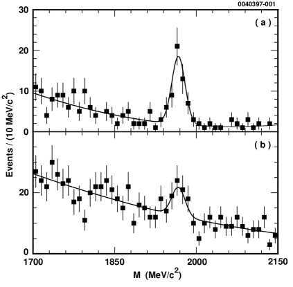
FIG. 1.: Histogram of (a) $\eta\pi^{+}$, and (b) $\omega\pi^{+}$ invariant mass for tagged events. The points with error bars are the data; the solid lines are the result of the constrained fit to the data, as described in the text.

Finally, we sorted the $D_{s}^{+}$ candidates into two categories: “tagged” and “untagged”. The tagged events are those that are consistent with coming from the decay $D^{*+}_{s}\to D_{s}^{+}\gamma$. To tag events, we combined the $D_{s}^{+}$ candidates with photons and calculated the invariant mass of each $D_{s}^{+}\gamma$ combination. To suppress mistags from energy clusters produced by hadronic interactions, we required the tagging photon’s energy be at least 250 MeV and its lateral shape to be consistent with an electromagnetic shower. We calculated the mass difference $\Delta M_{\gamma}\equiv M(D_{s}^{+}\gamma)-M(D_{s}^{+})$. The $D_{s}^{+}$ is “tagged” if 134 MeV/$c^{2}\leq\Delta M_{\gamma}<154$ MeV/$c^{2}$. Events in which no photon meets this criterion are “untagged”. The invariant mass distribution of the tagged $\eta\pi^{+}$ combinations is shown in Fig. 1a. The histogram has been fit with a Gaussian for the $D_{s}^{+}\to\eta\pi^{+}$ events and a second-order polynomial for the combinatoric background. The mean and width of the Gaussian were fixed to the values predicted by Monte Carlo. The fit finds $48.4^{+8.4}_{-7.7}$ signal events (statistical error only). The overlayed functions shown in the figure are the result of a more constrained fit described below. About 3% of the events contained more than one $\eta\pi^{+}$ combination which satisfied our criteria. The same is true in the $\omega\pi^{+}$ mode. Since this occurred at the same rate in the data and Monte Carlo, and in both the signal and normalizing modes, we accepted these double-counts; they have negligible effect on our results.

A histogram of the invariant mass of the tagged $\omega\pi^{+}$ combinations is shown in Fig. 1b. It was fit with the same functions as the $\eta\pi^{+}$ data, using the same Gaussian parameters, as predicted by the Monte Carlo. This fit finds $35.7^{+10.8}_{-10.2}\ D_{s}^{+}\to\omega\pi^{+}$ events (statistical error only). We consider this to be a significant signal and describe further tests of the data below.

A number of checks have been performed to help validate this signal. Three-pion combinations were selected in sidebands to the $\omega$ signal region: 670 MeV/$c^{2}\leq M(\pi^{+}\pi^{-}\pi^{0})<710$ MeV/$c^{2}$ and 855 MeV/$c^{2}\leq M(\pi^{+}\pi^{-}\pi^{0})<895$ MeV/$c^{2}$. When these are combined with a fourth pion, and the $\omega\pi^{+}$ selection criteria applied, no $D_{s}^{+}$ signal is seen in either sideband. To reproduce the observed $\omega\pi^{+}$ signal would require a 6 standard deviation fluctuation.

One can also fit the $\Delta M_{\gamma}$ distributions for a signal. Requiring that the four-pion ($\eta\pi^{+}$ or $\omega\pi^{+}$) mass be between 1943 and 1991 MeV/$c^{2}$ and removing the cut on $\Delta M_{\gamma}$, we found $50^{+10}_{-9}$ $\eta\pi^{+}$ events and $42^{+14}_{-13}$ $\omega\pi^{+}$ events, in good agreement with the yields found in the previous fits to the $\eta\pi^{+}$ and $\omega\pi^{+}$ mass distributions (Fig. 2). In these $\Delta M_{\gamma}$ histograms, double-counting occurred at a rate of about 10%; this is neglible compared to the statistical errors.

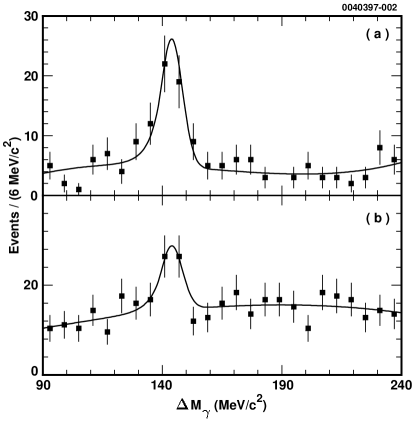
FIG. 2.: Histogram of $\Delta M_{\gamma}$ for (a) $\eta\pi^{+}$ events, and (b) $\omega\pi^{+}$ events. The points with error bars are the data. The solid lines are fits, using a modified Gaussian for the signal, whose shape was fixed using Monte Carlo events, and a third-order polynomial for the background.

To confirm that these events are in fact $D_{s}^{+}\to\omega\pi^{+}$, rather than some other four-pion decay of the $D_{s}^{+}$, we loosened the $\omega$ mass cut and took all $\pi^{+}\pi^{-}\pi^{0}$ combinations with masses between 650 and 900 MeV/$c^{2}$. These were then combined with a fourth pion; the four-pion combinations that passed the tagging criteria (and all other cuts) were kept. Again requiring that the four-pion mass be between 1943 and 1991 MeV/$c^{2}$, we made a histogram of the three-pion invariant mass. A fit to this histogram yields $44\pm 12$ events. However, there are also real $\omega$’s in the $\omega\pi^{+}$ random combinations under the $D_{s}^{+}$ peak. To account for this, we performed a sideband subtraction, using upper and lower sidebands in four-pion mass. After the subtraction, a fit to the three-pion invariant mass found $32\pm 12$ $\omega$’s, consistent with our previous results.

We have calculated the invariant mass of the “other” three pion combination in each $\omega\pi^{+}$ candidate event. We define ${M_{3}}^{\prime}$ to be the invariant mass of the bachelor $\pi^{+}$ with the $\pi^{-}$ and $\pi^{0}$ from the $\omega$. For the $\omega\pi^{+}$ events, all of the events in the $D_{s}^{+}$ signal region have ${M_{3}}^{\prime}>1100$ MeV/$c^{2}$. Thus these events are not simply $D_{s}^{+}\to\eta\pi^{+}$ or $D_{s}^{+}\to\phi\pi^{+}$ (with $\phi\to\pi^{+}\pi^{-}\pi^{0}$) events feeding into $\omega\pi^{+}$ by combining the pions in the “wrong” order. The ${M_{3}}^{\prime}$ distribution agrees with the signal Monte Carlo prediction.

Similarly, we reconstructed events in the signal region as $K^{-}\pi^{+}\pi^{+}\pi^{0}$, as might come from $D^{*+}$ decay, by assigning the kaon mass to the negatively-charged track. We found that the invariant mass for this alternate particle assignment in every case is more than 2040 MeV/$c^{2}$, so these cannot be misreconstructed $D^{*+}$ events. Again, the measured distribution agrees with the Monte Carlo prediction.

The untagged sample of $\omega\pi^{+}$ events contains a small excess at the $D_{s}^{+}$ mass (Fig. 3). A fit yields $133\pm 57$ signal events. Fitting the untagged $\eta\pi^{+}$ distribution finds $312\pm 31$ signal events. We included these untagged events in the branching ratio measurement.

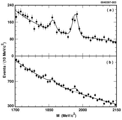
FIG. 3.: Histogram of (a) $\eta\pi^{+}$, and (b) $\omega\pi^{+}$ invariant mass for untagged events. The points with error bars are the data; the solid lines are the result of the constrained fit to the data, as described in the text. The fits include a Gaussian of fixed mean and width for $D^{+}$ events near 1869 MeV/$c^{2}$. In the lower plot, the dashed line shows the background function underneath the $D_{s}^{+}$ signal; the $y$-axis scale has been zero-suppressed.

The ratio of reconstruction efficiencies, $\epsilon(\omega\pi^{+})/\epsilon(\eta\pi^{+})$, is the same for tagged and untagged events, so the raw ratio of signal events should also be the same in both samples. For the tagged events, we find a ratio of $0.74\pm 0.25$  $\omega\pi^{+}$ event per $\eta\pi^{+}$ event. For the untagged events, the ratio is $0.43\pm 0.19$. The two ratios are statistically consistent.

We also performed a simultaneous fit to the four distributions ($\eta\pi^{+}$ and $\omega\pi^{+}$, tagged and untagged), and constrained the ratio of $\omega\pi^{+}$ to $\eta\pi^{+}$ events to be the same for both samples. This yielded a ratio of $0.56^{+0.15}_{-0.14}$; the $\chi^{2}$ of the fit to the four histograms was 146.8 with 161 degrees of freedom. We used the result of this constrained fit in the branching ratio calculation; the fit functions shown in figures 1 and 3 are also the result of this fit. Refitting the histograms with the number of $D_{s}^{+}\to\omega\pi^{+}$ events fixed to be zero yielded a $\chi^{2}$ of 166.9, an increase of 20.1.

Using the ratio of efficiencies determined from Monte Carlo and the $\eta$ and $\omega$ branching fractions to $\pi^{+}\pi^{-}\pi^{0}$[7], we determined the branching ratio:

$${\Gamma(D_{s}^{+}\to\omega\pi^{+})\over\Gamma(D_{s}^{+}\to\eta\pi^{+})}=0.16\pm 0.04\pm 0.03.$$ (1)

The first error is statistical; the systematic error is dominated by variations in the branching ratio caused by varying the cuts used in the analysis. These variations help gauge the accuracy of our event simulation. The systematic error also includes contributions from the uncertainty in the efficiencies, the branching fractions of the $\eta$ and $\omega$, and from variations in the result using different fitting functions.

In order to calculate an absolute branching fraction for $D_{s}^{+}\to\omega\pi^{+}$, we used the new CLEO measurement ${\Gamma(D_{s}^{+}\to\eta\pi^{+})/\Gamma(D_{s}^{+}\to\phi\pi^{+})}=0.47\pm 0.07\cite[cite]{[\@@bibref{Number}{CLEOETAPI}{}{}]},$ and the PDG value of $B(D_{s}^{+}\to\phi\pi^{+})=0.036\pm 0.009$[7]. This yields a branching fraction:

$$B(D_{s}^{+}\to\omega\pi^{+})=(2.7\pm 1.2)\times 10^{-3},$$ (2)

where all the errors have been added in quadrature. Thus we have observed the decay $D_{s}^{+}\to\omega\pi^{+}$, which may be the result of annihilation decay, final state interactions, or both.

We gratefully acknowledge the effort of the CESR staff in providing us with excellent luminosity and running conditions. This work was supported by the National Science Foundation, the U.S. Department of Energy, the Heisenberg Foundation, the Alexander von Humboldt Stiftung, Research Corporation, the Natural Sciences and Engineering Research Council of Canada, and the A.P. Sloan Foundation.

REFERENCES

- [1] Throughout this paper, reference to a particular charge state implies the inclusion of the charge-conjugate state as well.
- [2] Some theoretical papers made a sign error regarding this, and thus predicted a significant rate for decay to and a vanishing rate to ; for example, B. Yu. Blok and M. A. Shifman, Sov. J. Nucl. Phys. 45, 522 (1987) [Yad. Fiz. 45, 841 (1987)]; Sov. J. Nucl. Phys. 46, 767 (1987) [Yad. Fiz. 46, 1310 (1987)] and L-L. Chau and H-Y. Cheng, Phys. Lett. B222, 285 (1989); cf. reference 4.
- [3] A. N. Kamal, N. Sinha, & R. Sinha, Phys. Rev. D, 39, 3503 (1989).
- [4] H. J. Lipkin, “Symmetry, Topology and Helicity in and Decays,” in the Proceedings, International Symposium on Heavy Quark Physics, Ithaca, NY; edited by P. S. Drell and D. L. Rubin (1989).
- [5] F. Buccella, M. Lusignoli and A. Pugliese, Phys. Lett. B379, 249 (1996).
- [6] Fermilab E691 Collaboration, J. C. Anjos et al., Phys. Lett. B223, 267 (1989).
- [7] Particle Data Group, R. M. Barnett et al., Phys. Rev. D 54, 1 (1996).
- [8] CLEO Collaboration, D. Acosta et al., Phys. Rev. D 49, 5690 (1994); also WA75, S. Aoki et al., Progress of Theoretical Physics 89, 131 (1993); and BES, J. Z. Bai et al., Phys. Rev. Lett. 74, 4599 (1995).
- [9] CLEO Collaboration, J. Bartelt et al., CLEO CONF 96-19, ICHEP96 PA05-114 (1996).
- [10] CLEO Collaboration, Y. Kubota et al., Nucl. Instrum. Methods Phys. Res. Sect. A 320, 66 (1992).
- [11] The CLEO detector simulation is based on GEANT 3.14, R. Brun et al.. CERN Report No. CC/EE84-1 (unpublished).