Search for the Decays ${B^{0}}\!\to\!{D^{(*)+}}\,{D^{(*)-}}$

Abstract

Using the CLEO-II data set we have searched for the Cabibbo-suppressed decays ${B^{0}}\!\to\!{D^{(*)+}}\,{D^{(*)-}}$. For the decay ${B^{0}}\!\to\!{D^{*+}}\,{D^{*-}}$, we observe one candidate signal event, with an expected background of $0.022\pm 0.011$ events. This yield corresponds to a branching fraction of ${\cal B}({{B^{0}}\!\to\!{D^{*+}}\,{D^{*-}}})={{(5.3^{+7.1}_{-3.7}(\rm{stat})\pm 1.0(\rm{syst}))\times 10^{-4}}}$ and an upper limit of ${\cal B}({{B^{0}}\!\to\!{D^{*+}}\,{D^{*-}}})<{2.2\times 10^{-3}}$ at the $90\%$ CL. For ${B^{0}}\!\to\!{D^{*\pm}\,D^{\mp}}$ and ${B^{0}}\!\to\!{D^{+}}\,{D^{-}}$, no significant excess of signal above the expected background level is seen, and we calculate the $90\%$ CL upper limits on the branching fractions to be ${\cal B}({{B^{0}}\!\to\!{D^{*\pm}\,D^{\mp}}})<{1.8\times 10^{-3}}$ and ${\cal B}({{B^{0}}\!\to\!{D^{+}}\,{D^{-}}})<{1.2\times 10^{-3}}$.

D. M. Asner,¹ D. W. Bliss,¹ W. S. Brower,¹ G. Masek,¹ H. P. Paar,¹ V. Sharma,¹ J. Gronberg,² R. Kutschke,² D. J. Lange,² S. Menary,² R. J. Morrison,² H. N. Nelson,² T. K. Nelson,² C. Qiao,² J. D. Richman,² D. Roberts,² A. Ryd,² M. S. Witherell,² R. Balest,³ B. H. Behrens,³ K. Cho,³ W. T. Ford,³ H. Park,³ P. Rankin,³ J. Roy,³ J. G. Smith,³ J. P. Alexander,⁴ C. Bebek,⁴ B. E. Berger,⁴ K. Berkelman,⁴ K. Bloom,⁴ D. G. Cassel,⁴ H. A. Cho,⁴ D. M. Coffman,⁴ D. S. Crowcroft,⁴ M. Dickson,⁴ P. S. Drell,⁴ K. M. Ecklund,⁴ R. Ehrlich,⁴ R. Elia,⁴ A. D. Foland,⁴ P. Gaidarev,⁴ B. Gittelman,⁴ S. W. Gray,⁴ D. L. Hartill,⁴ B. K. Heltsley,⁴ P. I. Hopman,⁴ J. Kandaswamy,⁴ N. Katayama,⁴ P. C. Kim,⁴ D. L. Kreinick,⁴ T. Lee,⁴ Y. Liu,⁴ G. S. Ludwig,⁴ J. Masui,⁴ J. Mevissen,⁴ N. B. Mistry,⁴ C. R. Ng,⁴ E. Nordberg,⁴ M. Ogg,^4, J. R. Patterson,⁴ D. Peterson,⁴ D. Riley,⁴ A. Soffer,⁴ C. Ward,⁴ M. Athanas,⁵ P. Avery,⁵ C. D. Jones,⁵ M. Lohner,⁵ C. Prescott,⁵ S. Yang,⁵ J. Yelton,⁵ J. Zheng,⁵ G. Brandenburg,⁶ R. A. Briere,⁶ Y.S. Gao,⁶ D. Y.-J. Kim,⁶ R. Wilson,⁶ H. Yamamoto,⁶ T. E. Browder,⁷ F. Li,⁷ Y. Li,⁷ J. L. Rodriguez,⁷ T. Bergfeld,⁸ B. I. Eisenstein,⁸ J. Ernst,⁸ G. E. Gladding,⁸ G. D. Gollin,⁸ R. M. Hans,⁸ E. Johnson,⁸ I. Karliner,⁸ M. A. Marsh,⁸ M. Palmer,⁸ M. Selen,⁸ J. J. Thaler,⁸ K. W. Edwards,⁹ A. Bellerive,¹⁰ R. Janicek,¹⁰ D. B. MacFarlane,¹⁰ K. W. McLean,¹⁰ P. M. Patel,¹⁰ A. J. Sadoff,¹¹ R. Ammar,¹² P. Baringer,¹² A. Bean,¹² D. Besson,¹² D. Coppage,¹² C. Darling,¹² R. Davis,¹² N. Hancock,¹² S. Kotov,¹² I. Kravchenko,¹² N. Kwak,¹² S. Anderson,¹³ Y. Kubota,¹³ M. Lattery,¹³ J. J. O’Neill,¹³ S. Patton,¹³ R. Poling,¹³ T. Riehle,¹³ V. Savinov,¹³ A. Smith,¹³ M. S. Alam,¹⁴ S. B. Athar,¹⁴ Z. Ling,¹⁴ A. H. Mahmood,¹⁴ H. Severini,¹⁴ S. Timm,¹⁴ F. Wappler,¹⁴ A. Anastassov,¹⁵ S. Blinov,^15, J. E. Duboscq,¹⁵ K. D. Fisher,¹⁵ D. Fujino,^15, R. Fulton,¹⁵ K. K. Gan,¹⁵ T. Hart,¹⁵ K. Honscheid,¹⁵ H. Kagan,¹⁵ R. Kass,¹⁵ J. Lee,¹⁵ M. B. Spencer,¹⁵ M. Sung,¹⁵ A. Undrus,^15,† R. Wanke,¹⁵ A. Wolf,¹⁵ M. M. Zoeller,¹⁵ B. Nemati,¹⁶ S. J. Richichi,¹⁶ W. R. Ross,¹⁶ P. Skubic,¹⁶ M. Wood,¹⁶ M. Bishai,¹⁷ J. Fast,¹⁷ E. Gerndt,¹⁷ J. W. Hinson,¹⁷ N. Menon,¹⁷ D. H. Miller,¹⁷ E. I. Shibata,¹⁷ I. P. J. Shipsey,¹⁷ M. Yurko,¹⁷ L. Gibbons,¹⁸ S. D. Johnson,¹⁸ Y. Kwon,¹⁸ S. Roberts,¹⁸ E. H. Thorndike,¹⁸ C. P. Jessop,¹⁹ K. Lingel,¹⁹ H. Marsiske,¹⁹ M. L. Perl,¹⁹ S. F. Schaffner,¹⁹ D. Ugolini,¹⁹ R. Wang,¹⁹ X. Zhou,¹⁹ T. E. Coan,²⁰ V. Fadeyev,²⁰ I. Korolkov,²⁰ Y. Maravin,²⁰ I. Narsky,²⁰ V. Shelkov,²⁰ J. Staeck,²⁰ R. Stroynowski,²⁰ I. Volobouev,²⁰ J. Ye,²⁰ M. Artuso,²¹ A. Efimov,²¹ F. Frasconi,²¹ M. Gao,²¹ M. Goldberg,²¹ D. He,²¹ S. Kopp,²¹ G. C. Moneti,²¹ R. Mountain,²¹ Y. Mukhin,²¹ S. Schuh,²¹ T. Skwarnicki,²¹ S. Stone,²¹ G. Viehhauser,²¹ X. Xing,²¹ J. Bartelt,²² S. E. Csorna,²² V. Jain,²² S. Marka,²² A. Freyberger,²³ R. Godang,²³ K. Kinoshita,²³ I. C. Lai,²³ P. Pomianowski,²³ S. Schrenk,²³ G. Bonvicini,²⁴ D. Cinabro,²⁴ R. Greene,²⁴ L. P. Perera,²⁴ B. Barish,²⁵ M. Chadha,²⁵ S. Chan,²⁵ G. Eigen,²⁵ J. S. Miller,²⁵ C. O’Grady,²⁵ M. Schmidtler,²⁵ J. Urheim,²⁵ A. J. Weinstein,²⁵ and F. Würthwein²⁵

The decays ${B^{0}}\!\to\!{D^{(*)+}}\,{D^{(*)-}}$ are favorable modes for studying $CP$ violation in $B$ decays. In the Standard Model, time-dependent asymmetries in the decays can be related to the angle $\beta$ of the unitarity triangle [1]. This angle can also be measured with ${B^{0}}\!\to\!{\psi}\,{K^{0}_{S}}$ decays; any difference between the values obtained in ${B^{0}}\!\to\!{D^{(*)+}}\,{D^{(*)-}}$ decays and ${B^{0}}\!\to\!{\psi}\,{K^{0}_{S}}$ would indicate non-Standard Model mechanisms for $CP$ violation [2, 3]. Although ${B^{0}}\!\to\!{D^{*+}}\,{D^{*-}}$ and ${B^{0}}\!\to\!{D^{*\pm}\,D^{\mp}}$ are not pure $CP$ eigenstates, estimates indicate that a dilution of the $CP$ asymmetry of only a few percent would be incurred by treating these modes as pure $CP$ eigenstates [1].

The modes ${B^{0}}\!\to\!{D^{(*)+}}\,{D^{(*)-}}$ have never been observed, and no published limits on their branching fractions exist. The decay amplitude is dominated by a spectator diagram with $\bar{b}\to\bar{c}W^{+}$ followed by the Cabibbo-suppressed process $W^{+}\to c\bar{d}$. One can estimate the branching fractions for ${B^{0}}\!\to\!{D^{(*)+}}\,{D^{(*)-}}$ by relating them to the Cabibbo-favored decays ${B^{0}}\!\to\!{D^{(*)+}_{s}}\,{D^{(*)-}}$:

$${\cal B}({{B^{0}}\!\to\!{D^{(*)+}}\,{D^{(*)-}}}) \simeq \left(\frac{f_{D^{(*)}}}{f_{D_{s}^{(*)}}}\right)^{2}\tan^{2}\theta_{C}\ {\cal B}({{B^{0}}\!\to\!{D^{(*)+}_{s}}\,{D^{(*)-}}}),$$ (1)

where the $f_{X}$ are decay constants and $\theta_{C}$ is the Cabibbo angle. Table I shows the expected ${B^{0}}\!\to\!{D^{(*)+}}\,{D^{(*)-}}$ branching fractions, where the CLEO measurements of ${\cal B}({{B^{0}}\!\to\!{D^{(*)+}_{s}}\,{D^{(*)-}}})$ have been used [4].

TABLE I.: Estimated branching fractions for ${B^{0}}\!\to\!{D^{(*)+}}\,{D^{(*)-}}$ based on the measured branching fractions of the Cabibbo-favored decays ${B^{0}}\!\to\!{D^{(*)+}_{s}}\,{D^{(*)-}}$.

Mode	${\cal B}$ of Related	Estimated ${\cal B}$ for
	$D^{(*)+}_{s}$$D^{(*)-}$ Mode (%)	$D^{(*)+}$$D^{(*)-}$ ($10^{-4}$)
${B^{0}}\!\to\!{D^{*+}}\,{D^{*-}}$	2.4	9.7
${B^{0}}\!\to\!{D^{*\pm}\,D^{\mp}}$	2.0	8.1
${B^{0}}\!\to\!{D^{+}}\,{D^{-}}$	1.1	4.5

The data used in this analysis were recorded with the CLEO-II detector [5] located at the Cornell Electron Storage Ring (CESR). An integrated luminosity of $3.09~{}{\rm fb}^{-1}$ was taken at the $\Upsilon(4{\rm S})$ resonance, corresponding to approximately $3.3\times 10^{6}~{}{{B}{\bar{B}}}$ pairs produced.

At the $\Upsilon(4{\rm S})$, the $B$$\bar{B}$ pairs are produced nearly at rest, resulting in a spherical event topology. In contrast, non-$B$$\bar{B}$, continuum events have a more jet-like topology. To select spherical events we required that the ratio $R_{2}$ of the second and zeroth Fox-Wolfram moments [6] be less than 0.25.

We required charged tracks to be of good quality and consistent with coming from the interaction point in both the $r-\phi$ and $r-z$ planes. We defined photon candidates as isolated clusters in the CsI calorimeter with energy greater than 30 MeV in the central region ($\cos\theta\leq 0.71$, where $\theta$ is measured from the beamline) and greater than 50 MeV elsewhere. Pairs of photons with measured invariant masses within 2.5 standard deviations of the nominal $\pi^{0}$ mass were used to form $\pi^{0}$ candidates. Selected $\pi^{0}$ candidates were then kinematically fitted to the nominal $\pi^{0}$ mass.

A particle identification system consisting of $dE/dx$ and time-of-flight was used to distinguish charged kaons from charged pions. For charged pion candidates, we required the likelihood of the pion hypothesis, $L_{\pi}$, to be greater than 0.05. Since all signal modes require two charged kaons, the kaon candidates were required to have a joint kaon hypothesis likelihood, $L_{K_{1}}L_{K_{2}}$, greater than 0.10.

We reconstructed all $D^{*+}$ candidates in the mode ${D^{*+}}\!\to\!{\pi^{+}}\,{D^{0}}$ (charge-conjugate modes are implied). $D^{0}$ candidates were reconstructed in the modes ${D^{0}}\!\to\!{K^{-}}\,{\pi^{+}}$, ${D^{0}}\!\to\!{K^{-}}\,{\pi^{+}}\,{\pi^{0}}$ and ${D^{0}}\!\to\!{K^{-}}\,{\pi^{+}}\,{\pi^{-}}\,{\pi^{+}}$. $D^{+}$ candidates were reconstructed via ${D^{+}}\!\to\!{K^{-}}\,{\pi^{+}}$ $\pi^{+}$. Table II summarizes the branching fractions of the $D^{(*)}$ modes used [7].

TABLE II.: Branching fractions of $D^{(*)}$ modes used in reconstruction.

Decay Mode	Branching Fraction (%)
${D^{*+}}\!\to\!{\pi^{+}}\,{D^{0}}$	$68.3\pm 1.4$
${D^{0}}\!\to\!{K^{-}}\,{\pi^{+}}$	$3.83\pm 0.12$
${D^{0}}\!\to\!{K^{-}}\,{\pi^{+}}\,{\pi^{0}}$	$13.9\pm 0.9$
${D^{0}}\!\to\!{K^{-}}\,{\pi^{+}}\,{\pi^{-}}\,{\pi^{+}}$	$7.5\pm 0.4$
${D^{+}}\!\to\!{K^{-}}\,{\pi^{+}}$ $\pi^{+}$	$9.1\pm 0.6$

For the decay mode ${D^{0}}\!\to\!{K^{-}}\,{\pi^{+}}\,{\pi^{0}}$, we make a cut on the weight in the Dalitz plot in order to take advantage of the resonant substructure present in the decay. The cut choosen was 76% efficient for good ${D^{0}}\!\to\!{K^{-}}\,{\pi^{+}}\,{\pi^{0}}$ decays while rejecting 69% of the background.

We performed a vertex-constrained fit on all the charged tracks in the $B^{0}$ candidate for modes that contained a $D^{*+}$. The $\chi^{2}$ from the vertex fit was required to be less than 100. The fit improved the determination of the angular track parameters for the slow $\pi^{+}$ from the $D^{*+}$ decay. The resulting r.m.s. resolution on the reconstructed mass difference ${\Delta m_{{D^{*}}-{D}}}\equiv m_{{D^{*+}}}-m_{{D^{0}}}$ was approximately 0.69 MeV.

Because ${B^{0}}\!\to\!{D^{*\pm}\,D^{\mp}}$ is a $Pseudoscalar\to Vector+Pseudoscalar$ decay, the cosine of the decay angle, $\cos\theta_{\pi^{+}}$, of the slow $\pi^{+}$ from the $D^{*+}$ has a $\cos^{2}\theta$ distribution, while background events have a uniform distribution in this variable. For ${B^{0}}\!\to\!{D^{*\pm}\,D^{\mp}}$ candidates we required $|{\cos\theta_{\pi^{+}}}|>0.5$.

To select $B^{0}$ candidates that contain well-identified $D^{(*)}$s we combine the reconstructed $D^{(*)}$ masses into a single quantity, $\chi^{2}_{M}$. The definition of $\chi^{2}_{M}$ for each mode is given by

$$\chi^{2}_{M}({{D^{*+}}{D^{*-}}}) = {{\left(\frac{({\Delta m})_{1}-\langle{\Delta m}\rangle}{\sigma_{\Delta m}}\right)^{2}+\left(\frac{({\Delta m})_{2}-\langle{\Delta m}\rangle}{\sigma_{\Delta m}}\right)^{2}+}}$$ (3)

$${{\left(\frac{(m_{{D^{0}}})_{1}-\langle m_{{D^{0}}}\rangle}{\sigma_{m_{{D^{0}}}}}\right)^{2}+\left(\frac{(m_{{D^{0}}})_{2}-\langle m_{{D^{0}}}\rangle}{\sigma_{m_{{D^{0}}}}}\right)^{2}}}$$

$$\chi^{2}_{M}({{D^{*\pm}\,D^{\mp}}}) = {{\left(\frac{{\Delta m}-\langle{\Delta m}\rangle}{\sigma_{\Delta m}}\right)^{2}+\left(\frac{m_{{D^{0}}}-\langle m_{{D^{0}}}\rangle}{\sigma_{m_{{D^{0}}}}}\right)^{2}+\left(\frac{m_{{D^{+}}}-\langle m_{{D^{+}}}\rangle}{\sigma_{m_{{D^{+}}}}}\right)^{2}}}$$ (4)

$$\chi^{2}_{M}({{D^{+}}{D^{-}}}) = {{\left(\frac{(m_{{D^{+}}})_{1}-\langle m_{{D^{+}}}\rangle}{\sigma_{m_{{D^{+}}}}}\right)^{2}+\left(\frac{(m_{{D^{+}}})_{2}-\langle m_{{D^{+}}}\rangle}{\sigma_{m_{{D^{+}}}}}\right)^{2}}},$$ (5)

where the values in angle brackets represent the nominal values and the sigmas are the r.m.s. resolutions on the given quantity. We require $\chi^{2}_{M}({{D^{*+}}{D^{*-}}})<8.0$, $\chi^{2}_{M}({{D^{*\pm}\,D^{\mp}}})<4.0$ and $\chi^{2}_{M}({{D^{+}}{D^{-}}})<2.0$. From studies of Monte Carlo and regions in the data outside of the signal areas in other variables, we find that the backgrounds are uniform in $\chi^{2}_{M}$.

Since the energy of the $B^{0}$ is equal to the beam energy at CESR, we used the beam energy instead of the measured energy of the $B^{0}$ candidate to calculate the beam-constrained mass: ${m_{B}}=\sqrt{E_{beam}^{2}-{\bf p}_{B}^{2}}$. The r.m.s. resolution in $m_{B}$ for signal events, as determined from Monte Carlo, is $2.8$ MeV. In addition, the energy difference, ${\Delta E}\equiv E_{B}-E_{beam}$, where $E_{B}$ is the measured $B^{0}$ energy, was used to distinguish signal from background. The resolution in $\Delta E$ is 12 MeV after performing a mass-constrained fit that included the masses of all secondary particles ($D^{(*)}$ and $\pi^{0}$). The signal region in all modes was defined as $|{\Delta E}|<2\sigma_{{\Delta E}}$ and $|{m_{B}}-\langle{m_{B^{0}}}\rangle|<2\sigma_{{m_{B}}}$.

We used a Monte Carlo simulation of the CLEO-II detector to optimize all cuts. Since the number of observed signal events was expected to be small, all cuts were optimized to minimize the probability that the expected background level would fluctuate up to or beyond the expected signal level. For calculating the expected number of signal events during this optimization we assumed a branching fraction of 0.1% for all ${B^{0}}\!\to\!{D^{(*)+}}\,{D^{(*)-}}$ modes.

Using the cuts defined above, we determined the signal reconstruction efficiency using Monte Carlo. The reconstruction efficiency and single event sensitivity ($SES\equiv(\epsilon\ {\cal B}\ N_{{B}{\bar{B}}})^{-1}$, where $\epsilon$ is the detection efficiency, ${\cal B}$ is the product of the daughter branching fractions and $N_{{B}{\bar{B}}}$ is the number of $B$$\bar{B}$ pairs produced in the data set) for each mode are summarized in Table III. The systematic uncertainty on the $SES$ is dominated largely by uncertainties in the $D$ and $D^{*}$ branching fractions, and, due to the large mean multiplicity of the final states, the uncertainty in the tracking efficiency.

TABLE III.: Summary of reconstruction efficiencies and single event sensitivities for the three ${B^{0}}\!\to\!{D^{(*)+}}\,{D^{(*)-}}$ modes.

Mode	Efficiency, $\epsilon$	$SES\equiv(\epsilon\ {\cal B}\ N_{{B}{\bar{B}}})^{-1}$
	(%)	($10^{-4}$)
${B^{0}}\!\to\!{D^{*+}}\,{D^{*-}}$	1.86	$5.45\pm 0.99$
${B^{0}}\!\to\!{D^{*\pm}\,D^{\mp}}$	5.07	$3.79\pm 0.53$
${B^{0}}\!\to\!{D^{+}}\,{D^{-}}$	14.41	$2.52\pm 0.40$

The dominant background is due to random combinations from $B$$\bar{B}$ and continuum events. The Monte Carlo predicts that this background varies smoothly in $\Delta E$ and $m_{B}$ , and this is verified in the data. The $m_{B}$ distribution for data in $\Delta E$ sidebands ($50~{}{\rm MeV}\leq|{\Delta E}|\leq 400~{}{\rm MeV}$) varies smoothly with no peaking in the signal region. The same is true for the $\Delta E$ distribution for data with ${m_{B}}<5.27~{}{\rm GeV}$. To estimate the background in the signal region, we count the events in a sideband in the $\Delta E$-$m_{B}$ plane ($50~{}{\rm MeV}\leq|{\Delta E}|\leq 400~{}{\rm MeV}$; $5.2~{}{\rm GeV}\leq{m_{B}}\leq E_{beam}$) and multiply by the relative efficiencies of the signal and sideband regions determined from background Monte Carlo.

Figures 1, 2 and 3 show the resulting plots of $\Delta E$ vs. $m_{B}$ for the three modes. The signal region is indicated with a solid line, and the sideband region is indicated with a dotted line.

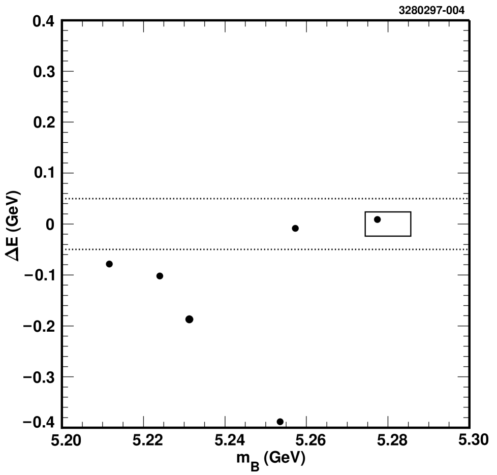
FIG. 1.: $\Delta E$ vs. $m_{B}$ for data in the ${B^{0}}\!\to\!{D^{*+}}\,{D^{*-}}$analysis. The signal region is indicated by a solid box. The sideband region lies above the top and below the bottom dotted lines.

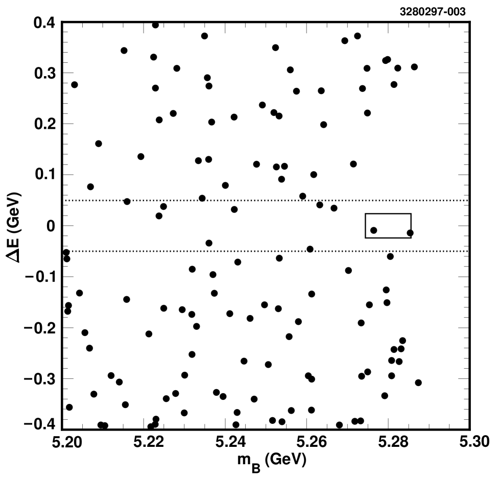
FIG. 2.: $\Delta E$ vs. $m_{B}$ for data in the ${B^{0}}\!\to\!{D^{*\pm}\,D^{\mp}}$analysis. The signal region is indicated by a solid box. The sideband region lies above the top and below the bottom dotted lines.

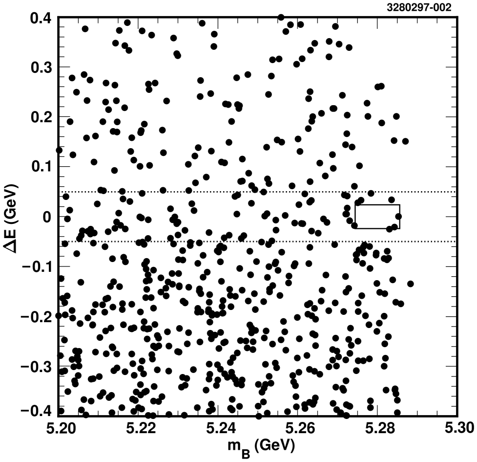
FIG. 3.: $\Delta E$ vs. $m_{B}$ for data in the ${B^{0}}\!\to\!{D^{+}}\,{D^{-}}$analysis. The signal region is indicated by a solid box. The sideband region lies above the top and below the bottom dotted lines.

Table IV lists the event yields in the sideband and signal regions. The expected number of background events in the signal region is also given. The uncertainty on the expected number of background events is a combination of statistical error on the number of events in the $\Delta E$ sideband regions and the uncertainty in the background shape through the signal region.

TABLE IV.: Summary of events found in the data, both in the $\Delta E$ sidebands and in the signal region, for each of the three modes.

Mode	Events in $\Delta E$	Predicted Background	Events found in
	Sidebands	in the Signal Region	Signal Region
${B^{0}}\!\to\!{D^{*+}}\,{D^{*-}}$	4	$0.022\pm 0.011$	1
${B^{0}}\!\to\!{D^{*\pm}\,D^{\mp}}$	117	$0.64\pm 0.10$	2
${B^{0}}\!\to\!{D^{+}}\,{D^{-}}$	539	$2.64\pm 0.34$	3

The probability that the expected background of $0.022\pm 0.011$ events in ${B^{0}}\!\to\!{D^{*+}}\,{D^{*-}}$ fluctuates up to one or more events is 2.2%. If we interpret the one observed event as evidence for a signal, the resulting branching fraction would be

$${\cal B}({{B^{0}}\!\to\!{D^{*+}}\,{D^{*-}}})={(5.3^{+7.1}_{-3.7}(\rm{stat})\pm 1.0(\rm{syst}))\times 10^{-4}},$$ (6)

where the systematic uncertainty comes from the uncertainty in the $SES$.

No significant excess of events is seen in the other two modes. We calculate upper limits on the branching fractions for all three modes, and these results are summarized in Table V. The systematic uncertainty in the $SES$ and the uncertainty in the background level have been incorporated into the upper limits [8].

TABLE V.: Summary of upper limits on the ${B^{0}}\!\to\!{D^{(*)+}}\,{D^{(*)-}}$ branching fractions. All upper limits are quoted at the 90% confidence level.

Mode	Upper Limit (90% CL)
${B^{0}}\!\to\!{D^{*+}}\,{D^{*-}}$	$2.2\times 10^{-3}$
${B^{0}}\!\to\!{D^{*\pm}\,D^{\mp}}$	$1.8\times 10^{-3}$
${B^{0}}\!\to\!{D^{+}}\,{D^{-}}$	$1.2\times 10^{-3}$

We have performed a search for the decays ${B^{0}}\!\to\!{D^{(*)+}}\,{D^{(*)-}}$. In the mode ${B^{0}}\!\to\!{D^{*+}}\,{D^{*-}}$, one event is seen in the signal region where the expected background is $0.022\pm 0.011$. The one event in ${B^{0}}\!\to\!{D^{*+}}\,{D^{*-}}$ is seen at a rate that is consistent with predictions, and in all three modes the upper limits are within about a factor of two from the predicted branching fractions.

- [1] R. Aleksan et al., Phys. Lett. B317, 173 (1993).
- [2] The BaBar Collaboration, Technical Design Report, SLAC-R-95-457 (1995).
- [3] K. Lingel et al., “Physics Rationale for a B Factory”, CLNS 91-1043 (1991).
- [4] CLEO Collaboration, D. Gibaut et al., Phys. Rev. D 53, 4734 (1996).
- [5] CLEO Collaboration, Y. Kubota et al., Nucl. Instrum. Methods A 320, 66 (1992).
- [6] G. Fox and S. Wolfram, Phys. Rev. Lett. 41, 1581 (1978).
- [7] Particle Data Group, R. M. Barnett et al., Phys. Rev. D 54, 1 (1996).
- [8] R. D. Cousins and V. Highland, Nucl. Instrum. Methods A 320, 331 (1992).