Erez Etzion

July 1994

.

.

The research work for this thesis was carried out
in the Experimental High Energy Group
of the School of Physics and Astronomy
under the supervision of Prof. Gideon Alexander

.

Abstract

This thesis describes a new a measurement of the tau lepton polarization and its forward-backward asymmetry at the Z⁰  resonance using the OPAL detector. This measurement is based on analyses of the $\tau$$\rightarrow$e$\bar{\nu}_{e}$$\nu_{\tau}$ , $\tau$$\rightarrow$$\mu$$\bar{\nu}_{\mu}$$\nu_{\tau}$ and $\tau$$\rightarrow$$\pi$(K)$\nu_{\tau}$ decays from a sample of $30663$ e⁺e^- $\rightarrow$$\tau^{+}$$\tau^{-}$ events collected in the polar angle range of $\mbox{$|\cos\theta|$}<0.68$ during the 1990-1992 data taking period. Taking then the Standard Model with the V–A structure of the tau lepton decay, we measure the average $\tau$ polarization to be

$$\mbox{$\langle P_{\tau}\rangle$}=(-13.5\pm 2.9\pm 2.2)\%$$

and the $\tau$ polarization forward-backward asymmetry to be

$$\mbox{\rm A${}_{pol}^{FB}$}=(-11.0\pm 3.5\pm 0.5)\%$$

where the first error is statistical and the second systematic. Combining these figures with the OPAL $\langle P_{\tau}\rangle$ and A${}_{pol}^{FB}$ measured with the $\tau$$\rightarrow$$\rho$$\nu_{\tau}$ channel we get an average $\tau$ polarization,

$$\mbox{$\langle P_{\tau}\rangle$}=(-14.9\pm 1.9\pm 1.3)\%$$

and for the asymmetry in the polarization,

$$\mbox{\rm A${}_{pol}^{FB}$}=(-8.9\pm 2.2\pm 0.9)\%$$

These results are consistent with lepton universality. Combining the two results we obtain for the electroweak mixing angle the value

$$\mbox{$\sin^{2}\theta_{W}^{\mbox{\small\it eff}}$}=0.2331\pm 0.0023$$

within the context of the Standard Model, where the error includes both statistical and systematic uncertainties.

Contents

1. 1 Introduction
2. 2 The LEP Accelerator
   1. 2.1 General Features
   2. 2.2 Luminosity
   3. 2.3 The Injection Chain
3. 3 The OPAL Detector
   1. 3.1 The Central Detector
   2. 3.2 The Electromagnetic Calorimeter
   3. 3.3 The Hadron Calorimeter
   4. 3.4 The Muon Detector
   5. 3.5 The Forward Detector
   6. 3.6 The Silicon Tungsten Detector
   7. 3.7 The Trigger
   8. 3.8 Online Dataflow
4. 4 Theoretical Background
   1. 4.1 A Brief Review of the Standard Model
   2. 4.2 The $\tau$-Asymmetry Formalism
   3. 4.3 The Charged Weak Decay Structure
   4. 4.4 Correlations Between A_FB, $\langle P_{\tau}\rangle$ and A${}_{pol}^{FB}$
   5. 4.5 The Fit Method
5. 5 Data Selection
   1. 5.1 Data
   2. 5.2 Monte Carlo and Control Samples
   3. 5.3 Tau Pair Selection
   4. 5.4 Tau Decay Identification
6. 6 Physics Analysis
   1. 6.1 The Fit Procedure
   2. 6.2 Radiative and Threshold Effects
   3. 6.3 Detector Resolution
   4. 6.4 Tau-Pair Selection Efficiency
   5. 6.5 Efficiencies of the $\tau$ Decay Identification
   6. 6.6 Background
7. 7 Results and Cross Checks
   1. 7.1 Maximum Likelihood Fit Results
   2. 7.2 Summary of Systematic Studies
   3. 7.3 Monte Carlo checks
   4. 7.4 Cross Checks
   5. 7.5 $\langle P_{\tau}\rangle$  and A${}_{pol}^{FB}$  from $\tau$$\rightarrow$$\rho$$\nu_{\tau}$  decays
   6. 7.6 Comparison With Previous Measurements
8. 8 Summary

List of Figures

1. 2.1 A schematic layout of the LEP storage ring.
2. 2.2 LEP injection chain
3. 3.1 A schematic view of the OPAL detector.
4. 4.1 Feynman diagrams for the $\tau$ pair production
5. 4.2 The average tau polarization as a function of the polar angle.
6. 4.3 $\tau^{-}$ and $\tau^{+}$ decay into leptons .
7. 4.4 $\tau$$\rightarrow$$\ell$$\bar{\nu}_{\ell}$$\nu_{\tau}$ decay in the $\tau$ rest frame ( $x=1$)
8. 4.5 $\tau$$\rightarrow$$\ell$$\bar{\nu}_{\ell}$$\nu_{\tau}$ decay in the $\tau$ rest frame (low $x$)
9. 4.6 $\tau$$\rightarrow$$\pi$(K)$\nu_{\tau}$  decay and the $\tau$ helicity orientation.
10. 4.7 The momentum distribution of $\tau$$\rightarrow$$\ell$$\bar{\nu}_{\ell}$$\nu_{\tau}$ and $\tau$$\rightarrow$$\pi$(K)$\nu_{\tau}$.
11. 4.8 The $\tau$ asymmetries as a function of the Weinberg mixing angle.
12. 4.9 The $\tau$ asymmetries as a function of $E_{cm}$
13. 5.1 Comparison of 1990+1991 with 1992 data samples.
14. 5.2 Comparison of 1990+1991 with 1992 data samples.
15. 5.3 Comparison of MC samples of 1991 with 1992 detector setups.
16. 5.4 Comparison of MC samples of 1991 with 1992 detector setups.
17. 5.5 $E_{cm}$ distribution of the data.
18. 5.6 Global efficiencies as a function of $x$.
19. 5.7 A display of a typical $\tau^{+}$$\tau^{-}$ event in the OPAL detector.
20. 6.1 Radiative corrections and the Born term expectation.
21. 6.2 Parametrization of the finite $\mu$ mass effect.
22. 6.3 Momentum resolution in $\tau$$\rightarrow$$\pi$(K)$\nu_{\tau}$ MC
23. 6.4 Momentum resolution in $\tau$$\rightarrow$$\mu$$\bar{\nu}_{\mu}$$\nu_{\tau}$ MC
24. 6.5 The resolution ${\cal R}(x,\mbox{$x$})$ as a function of $y_{\pi}$.
25. 6.6 The resolution ${\cal R}(x,\mbox{$x$})$ as a function of $y_{\mu}$.
26. 6.7 $x$ vs. $\cos\theta$ for data $\mu$-pairs.
27. 6.8 $\Delta E/E$ dependence on $x$.
28. 6.9 The energy resolution as a function of $y_{e}$.
29. 6.10 Tau-pair selection efficiencies as functions of $x$.
30. 6.11 Efficiencies of $\tau$$\rightarrow$e$\bar{\nu}_{e}$$\nu_{\tau}$ and $\tau$$\rightarrow$$\pi$(K)$\nu_{\tau}$ identification.
31. 6.12 Efficiencies of $\tau$$\rightarrow$$\mu$$\bar{\nu}_{\mu}$$\nu_{\tau}$ identification (I).
32. 6.13 Efficiencies of $\tau$$\rightarrow$$\mu$$\bar{\nu}_{\mu}$$\nu_{\tau}$ identification (II).
33. 6.14 Data corrections to the efficiencies for the tau identification
34. 6.15 Background from other tau decays as functions of $x$.
35. 6.16 Background from other tau decays as functions of $|\cos\theta|$.
36. 6.17 Background from non-tau sources.
37. 7.1 Measurement of $\langle P_{\tau}\rangle$ in MC with different input $\langle P_{\tau}\rangle$.
38. 7.2 MC $x$ distributions of the $\tau$$\rightarrow$e$\bar{\nu}_{e}$$\nu_{\tau}$ decay channel.
39. 7.3 MC $x$ distributions for the $\tau$$\rightarrow$$\mu$$\bar{\nu}_{\mu}$$\nu_{\tau}$ decay channel.
40. 7.4 MC $x$ distributions of the $\tau$$\rightarrow$$\pi$(K)$\nu_{\tau}$ decay channel.
41. 7.5 MC $x$ distributions of the $\tau$$\rightarrow$e$\bar{\nu}_{e}$$\nu_{\tau}$, $\tau$$\rightarrow$$\mu$$\bar{\nu}_{\mu}$$\nu_{\tau}$ and $\tau$$\rightarrow$$\pi$(K)$\nu_{\tau}$.
42. 7.6 $x$ distributions of the $\tau$$\rightarrow$e$\bar{\nu}_{e}$$\nu_{\tau}$ decay channel
43. 7.7 $x$ distributions of the $\tau$$\rightarrow$$\mu$$\bar{\nu}_{\mu}$$\nu_{\tau}$ decay channel
44. 7.8 $x$ distributions of the $\tau$$\rightarrow$$\pi$(K)$\nu_{\tau}$ decay channel
45. 7.9 $x$ distributions of the $\tau$$\rightarrow$e$\bar{\nu}_{e}$$\nu_{\tau}$, $\tau$$\rightarrow$$\mu$$\bar{\nu}_{\mu}$$\nu_{\tau}$ and $\tau$$\rightarrow$$\pi$(K)$\nu_{\tau}$ decays.
46. 7.10 Tau polarization as function of $\cos\theta$.
47. 7.11 LEP 1990-1992  $\langle P_{\tau}\rangle$ and A${}_{pol}^{FB}$ (preliminary) results
48. 8.1 Comparison of several determinations of the weak mixing angle

List of Tables

1. 2.1 Integrated luminosity in OPAL.
2. 2.2 The design LEP parameters.
3. 4.1 The leptons weak coupling constants.
4. 4.2 The Michel parameters for some different $V$ and $A$ combinations
5. 4.3 The correlation coefficients between $\tau$- asymmetries.
6. 4.4 An estimate of the $\tau$  asymmetries statistical errors
7. 4.5 An estimate of the $\tau$  asymmetries correlations
8. 4.6 The errors in the $\tau$ asymmetries for different fit approachs
9. 4.7 Estimated errors for events where both decays are identified
10. 4.8 Estimated correlations for events where both decays are identified
11. 5.1 Detector and trigger status requirements.
12. 5.2 $\tau$-pair events classified according to their identification
13. 6.1 Forward-backward asymmetries.
14. 6.2 Systematic errors associated with radiative effects.
15. 6.3 Parametrization of the finite $\mu$-mass effect.
16. 6.4 MC detector response parametrization
17. 6.5 Parameterization of the $x$ resolution of pions.
18. 6.6 Parameterization of the $x$ resolution of muons.
19. 6.7 Systematic errors of $\mu$ and $\pi$ resolution function
20. 6.8 Parameters of the electron energy resolution functions.
21. 6.9 Systematic errors associated with electron resolution function.
22. 6.10 $\chi^{2}/D.O.F.$ of the $\tau$-pair selection efficiency fits.
23. 6.11 Systematic errors associated with $\tau$-pair selection efficiency.
24. 6.12 $\chi^{2}/D.O.F.$ of the $\tau$ decay identification fits.
25. 6.13 Systematic errors associated with $\tau$ decay identification
26. 6.14 Tau branching fractions.
27. 6.15 Background fractions from the various sources.
28. 6.16 Systematic errors of background from other tau decays
29. 6.17 Non-tau background sources.
30. 6.18 Systematic errors associated with the non-tau background.
31. 7.1 Summary of systematic uncertainties.
32. 7.2 Polarization results in MC sample.
33. 7.3 Results for the nine independent subsamples.
34. 7.4 Tau polarization results calculated by $\chi^{2}$ fit.
35. 7.5 $\tau$ polarization results.
36. 7.6 LEP 1990-1992  $\langle P_{\tau}\rangle$ and A${}_{pol}^{FB}$ (preliminary) results
37. 8.1 OPAL combined $\tau$ polarization results.

.

Chapter 1 Introduction

One of the central phenomena characterizing weak interactions is the non-conservation of parity. This effect, originally established for weak charged-current interactions, is also embedded in the Standard Model [1, 2, 3] to exist in neutral-current interactions, resulting in different Z⁰ couplings to left-handed and right-handed fermions. Consequently, the Z⁰ boson produced by e⁺e^- annihilation is expected to be polarized because of its different couplings to the incoming left-handed and right-handed electrons. Similarly, fermions produced in Z⁰ decay are expected to have a degree of polarization depending on their coupling constants. Another consequent of this Z⁰ polarization is a forward-backward asymmetry in the polarization of the outgoing fermions. Hence, some of the best Standard Model tests in the annihilation of $e^{+}e^{-}$ at the Z⁰ pole provided by the following asymmetries measurements:

• The Forward Backward asymmetry, A_FB, which can be measured in all the $e^{+}e^{-}\to f\bar{f}$ channels.

• The Left Right Asymmetry, $A_{LR}$, which can be measured in the annihilation of longitudinal polarized $e^{+}e^{-}$ beams (at the moment available only at SLAC’s SLD experiment).

• The Final Lepton Polarization Asymmetry, $\langle P_{f}\rangle$ which can be measured only in the $\tau$ decay ($\langle P_{\tau}\rangle$).

• The Forward Backward Asymmetry in the Lepton Polarization, A${}_{pol}^{FB}$, which again can be measured only in the $\tau$ decay .

The $\langle P_{\tau}\rangle$ and the A${}_{pol}^{FB}$ asymmetries can be studied in the process e⁺e^- $\rightarrow$$\tau^{+}$$\tau^{-}$  using the energy distribution of the $\tau$ decay products in the laboratory frame [4].

The mixing angle between the electromagnetic and the weak interaction, $\sin^{2}\theta_{W}$, plays a central role in the theory of the Standard Model. Being so it is measured by the LEP experiments in several processes and by various methods. The Standard Model gives predictions for A_FB, $\langle P_{\tau}\rangle$ and A${}_{pol}^{FB}$ as a functions of $s=\mbox{$E_{cm}$}^{2}$ in terms of the Z⁰ parameters (mass and width) and its vector ($v_{l}$) and axial-vector ($a_{l}$) couplings to the electron and the tau. Using the improved Born approximation [5] which accounts for most weak radiative corrections, our measurements of $\langle P_{\tau}\rangle$ and A${}_{pol}^{FB}$ provide a test of e-$\tau$ universality in the neutral current which is independent of lepton universality tests performed by studying the line shapes and the forward-backward asymmetries of the Bhabha, $\mu$-pair and $\tau$-pair cross-sections [6].

Our results supercede OPAL’s first $\tau$ polarization measurements [7] which was based solely on the 1990 data. The other LEP collaborations have also reported their measurements of the $\tau$ polarization [8]-[13] forward-backward asymmetry [11]-[13], based on their 1990 and 1991 data.

The present thesis describes a measurement of the $\tau$ polarization,  $\langle P_{\tau}\rangle$, and its forward-backward asymmetry,  A${}_{pol}^{FB}$, using the $\tau$-pair events collected with the OPAL detector at LEP during the period 1990-1992. It is based on a sample of 30663 e⁺e^- $\rightarrow$$\tau^{+}$$\tau^{-}$ events which were detected within the polar angle range of $|\cos\theta|<0.68$. Most of these events (91.5%) were measured on the Z⁰ peak and the remainder at center-of-mass energies ($E_{cm}$) of 1, 2, and 3  $GeV$ below and above the peak of Z⁰ resonance. The decay channels $\tau$$\rightarrow$e$\bar{\nu}_{e}$$\nu_{\tau}$, $\tau$$\rightarrow$$\mu$$\bar{\nu}_{\mu}$$\nu_{\tau}$ and $\tau$$\rightarrow$$\pi$(K)$\nu_{\tau}$ are used.

These results combined with the analysis of the $\tau$$\rightarrow$$\rho$$\nu_{\tau}$ decay channel [14, 15] were presented as an OPAL publication [17, 16]. Therefore for the sake of completeness we present here also the combined results.

The analysis is based on an event-by-event Maximum Likelihood fit to the theoretical energy distributions of the $\tau$ decay product. The energy is corrected for radiative effects and detector response, in which all correlations between the two tau decays are taken into account. We apply our ‘global fit’ method to the three $\tau$ decay channels from which the polarization is extracted using distributions in simple observables. This method has the advantage of taking explicitly into account the correlations between polarization observables of the two taus introduced by the selection and identification criteria. This is particularly important for the leptonic channels where requirements are made on the whole event in order to suppress backgrounds from Bhabha and mu-pair events. In addition, the method correctly extracts information using the tau-tau spin correlations in those events where both taus have identified decays.

The thesis is organized as follows: A description of the LEP accelerator and the OPAL detector are presented in the following two Chapters. A brief description of the Standard Model and a discussion of the polarization formalism, are given in the Chapter 4. It includes the definition of the various observables used in this analysis and the relations between them.

Chapter 5 presents the data and Monte Carlo samples used in the analysis, the event selection and $\tau$-decay identification. Chapter 6 describes the fit procedure and all the corrections used in our analysis, starting with radiative effects (Sect. 6.2), detector resolution (Sect. 6.3), $\tau$-pair selection efficiency (Sect. 6.4), $\tau$ decay identification efficiency (Sect. 6.5), and completing this list with background from other $\tau$ decay channels (Sect. 6.6.1) and from non-$\tau$ events (Sect. 6.6.2). Each correction is described along with the associated systematic studies. The results, including a summary of the systematic errors, and a presentation of the consistency checks done on the analysis, are included in Chapter 7. Finally the analysis is summarized in Chapter 8.

Chapter 2 The LEP Accelerator

2.1 General Features

The electrons and positrons which annihilate in the experiment are produced in the Large Electron Positron ring LEP, the current worlds largest $e^{+}e^{-}$ collider [19]-[22]. At the present stage LEP-I can provide colliding beams of energies upto $\sim 47$ $GeV$. With the machine upgrade planed for the next years LEP-II will accelerate the beam to $\sim 100$ $GeV$. The circumference of LEP is 26.66 $km$, partly in France and partly in Switzerland. The collider tunnel lies between about 43 $m$ and 140 $m$ below the surface. As injectors, LEP uses existing CERN machines. The LEP ring, has four interaction regions and was designed to reach a maximum luminosity of about L $\sim 1.7\times 10^{31}~{}cm^{-2}s^{-1}$ at a center of mass energy around $\mbox{$E_{cm}$}=90$ $GeV$. The storage ring has eight long straight sections, four of which are used for the particle physics experiments: L3, ALEPH, OPAL, and DELPHI. Fig. 2.1 shows a schematic layout of the LEP installations. The construction of LEP and its four detectors were completed in July 1989, and the first $Z^{0}$ event was seen in OPAL on the $13^{th}$ of August 1989.

2.1.1 Structure

The LEP storage ring is constructed out of four basic types of components, namely:

• The arc. The arc bends the beam in a circle and focuses it at the same time. These regions consists of regular arrays of quadrupoles and bending magnets, and most of the beam parameters are determined by its optics.

• Dispersion suppressor. Particles with different energies have different orbits in the ring. This can increase the beam size in the interaction point which reduces the luminosity. In order to avoid the luminosity reduction the dispersion suppressor are introduced in the RF section and in the low beta insertion.

• RF cavities. The function of it is to replace the energy lost by the particles through synchrotron radiation and other effects, and to provide a phase focussing.

• Interaction region. In theses regions the two beams collide. In order to get a high rate of interactions the beams are strongly focussed at these collision points. This is obtained by the low beta quadrupoles and a set of additional electro-magnetic lenses which optically match the insertion to the rest of the machine.

The focussing and bending property of the beam optics leads to two effects. First, a particle with nominal energy but with an uncertainty in position $\Delta x$ and/or in angle $\Delta\varphi$, will get focussed toward the nominal orbit and oscillate around it. This oscillation is called the betatron oscillation and it has the form

$$x(\ell)=\alpha\sqrt{\beta(\ell)}\cos(\phi(\ell)+\phi_{0}).$$ (2.1)

.

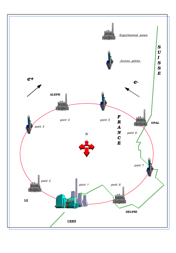
Figure 2.1: A schematic layout of the LEP storage ring. Point 1 is the injection point, while the even points are the four detectors: L3, ALEPH, OPAL, and DELPHI. The circumference of this ring is 26.6$~{}km$ and it lies between $43~{}m$ and $140~{}m$ under the ground.

where $\ell$ is the longitudinal position in the ring. The square root of the periodic function $\beta(\ell)$ gives the envelope of the betatron oscillation over many turns. The $\beta$ function value is large in a focussing quadrupole and small in a defocussing one.

The additional properties of the focussing and bending is to restrict the particles to an energy region $\Delta$E around the nominal energy . On one hand such particles with an excess energy do bend less in the dipole magnets, but on the other hand they go off center through the quadrupoles and therefore receive an extra bending. The result is, that the off-energy closed orbit particles have a horizontal displacement $\Delta x_{h}$

$$\Delta x_{h}=D_{x}\frac{\Delta E}{E}$$ (2.2)

where $D_{x}$ is called the periodic dispersion, and is a function of the longitudinal position in the ring, $D_{x}=D_{x}(\ell)$. The dispersion is typically large at the horizontally focussing quadrupoles and typically small at the defocussing ones. In LEP it is arranged so that the dispersion vanishes in all the straight sections by using proper transition to the arc, namely, the dispersion suppressors. In the arc section, where there is a finite dispersion, the deviation of the circumference is proportional to the energy deviation. The RF acceleration works in such a periodic function that a particle with an excess energy, which has a longer path length than a nominal energy one, will arrive later to the RF voltage area. In its time of arrival the voltage is smaller, and therefore it will suffer an energy loss. All this leads to oscillation around a Gaussian equilibrium of the LEP particles in their energy, longitudinal position, and transverse angle and position.

2.2 Luminosity

The reaction rate is proportional to the luminosity, $L$, and the reaction cross section, $\sigma$. The luminosity is a machine parameter, given by:

$$L=\frac{N^{2}kf_{0}}{4\pi\sigma_{x}\sigma_{y}}$$ (2.3)

where $N$ is the number of particles per bunch, $k$ the number of bunches,$f_{0}$ the revolution frequency and $\sigma_{x}$ and $\sigma_{y}$ the RMS values of the transverse radii at the collision points.

However there is an important limitation imposed by the beam-beam effect, due to the electromagnetic forces between the electrons and the positrons in the two crossing beams. This force has a linear part which leads to a change of the betatron frequency called the beam-beam tune shift. The particles oscillating with small amplitudes compared to $\sigma_{x}$ and $\sigma_{y}$ at the interaction points, suffer from the largest change in their tune. This shift is given by:

$$\xi_{i}=\frac{Nr_{e}\beta_{i}}{2\pi y\sigma_{x}(\sigma_{x}+\sigma_{i})}$$ (2.4)

where the index $i$ stands for $x$ or $y$, $r_{e}$ is the classical electron radius, $\beta_{x}$ and $\beta_{y}$ are the transverse beta function at the crossing points. It turns out that for most storage rings experiments, that the upper limit on $\xi_{y}$ is between 0.03 and 0.06. To optimize the luminosity estimation we can choose a tune shift as large as possible and this leaves us with

$$L=\frac{Nf_{0}k_{y}\xi_{y}}{2r_{e}\beta_{y}}.$$ (2.5)

Therefore, the experimental collision points are arranged in low $\beta$ insertions where $\beta_{x}$ and $\beta_{y}$ are much smaller than in the rest of LEP, namely that $\sigma_{x}$ and $\sigma_{y}$ become a fraction of a millimeter.

The cross section $\sigma$ is a property of the reaction itself, and one often compares it to the QED process $e^{+}e^{-}\stackrel{{\scriptstyle\gamma}}{{\rightarrow}}\mu^{+}\mu^{-}$. The cross section to this process decreases with $1/s$. It value is $\sim 10^{-35}~{}cm^{2}$ when $E_{beam}=M_{Z}/2$, which means that with a typical LEP luminosity of $10^{31}~{}cm^{-2}s^{-1}$ one will obtain a Z⁰ counting rate of $\sim 0.36~{}hour^{-1}$. On the $Z^{0}$ mass the main annihilation channel is via the formation of Z boson, $e^{+}e^{-}\stackrel{{\scriptstyle Z^{0}}}{{\rightarrow}}X$, with a cross section higher by a factor of $5\times 10^{3}$ than the propagation via a $\gamma$. Thus we expect on the peak about 1800 events per hour.

A typical luminosity for LEP during 1990 was about $0.4\times 10^{31}~{}cm^{-2}s^{-1}$ at the beginning of a fill. This leads to an average of one multihadronic event every $8~{}sec$, forward Bhabha event every $5~{}sec$, and $Z^{0}$ decay into charge leptons every $50~{}sec$. The Z⁰  production rate has further increased in the following years as can be seen in Table 2.1 which gives the OPAL integrated luminosity in the years 1990-1992. In 1993 the four LEP experiments together saw 3 million Z⁰ s, making a total of some 8 million since LEP began operating.

Year	Int. luminosity	No. of MH
1990	5.637 $pb^{-1}$	147425
1991	12.236 $pb^{-1}$	353324
1992	21.6319 $pb^{-1}$	767156

Table 2.1: The integrated luminosity and the number of MH events measured with the OPAL detector in the years 1990-1992.

2.2.1 Energy Loss Due to Synchrotron Radiation

The energy and the number of particles in a bunch are both limited by the synchrotron radiation. Electrons and positrons circulating in an orbit with radius $\rho$ lose energy due to synchrotron radiation. This loss per turn is given by:

$$U_{s}=\frac{4\pi}{3}\frac{r_{e}m_{0}c^{2}E^{4}}{\rho}$$ (2.6)

where $\rho$ is the bending radius of the arc which is 3096 $m$ in LEP. From this follows that the energy loss is 140 $MeV$ and 2330 $MeV$ for LEP operated at energies of 47 $GeV$ and 95 $GeV$ respectively. This loss has to be replaced by the RF system. The RF requirements are dominated by the losses in the cavities, which in storage rings increase with the beam energy. Therefore, synchrotron radiation causes sharp upper limits on both current and energy.

2.3 The Injection Chain

.

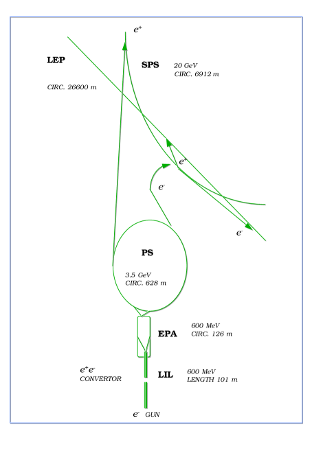
Figure 2.2: Injection into LEP. The LIL output are $600~{}MeV$ electrons and positrons. The EPA transfer the $e^{-}$ and $e^{+}$ as appropriate into the $3.5~{}GeV$ PS ring. From the PS the $e^{-}$ and $e^{+}$ are injected to the SPS ring where they are accelerated to $20~{}GeV$, and finally injected into LEP in eight equally spaced bunches of electrons and positrons.

The scheme for injection into LEP is shown in Fig. 2.2. An electron linac (LINear ACcelerator) which is a high current, 200 $MeV$ machine producing an output current of 2.5 $A$ for electron-to-positron conversion in a tungsten target. From there a positron current of 12 $mA$ is produced in a form suitable for subsequent acceleration in another linac which is used to accelerate these positrons up to an energy of 600 $MeV$. The first linac is also used to provide electrons for LEP by detuning its electron gun to produce 110 $mA$ at the linac output for acceleration to 600 $MeV$ in the second linac. The next stage in this chain is transferring the electrons or positrons, as appropriate, into an electron-positron accumulator ring (EPA) where they are stored and accumulated before injection into the Proton Synchrotron (PS). Acceleration to 3.5 $GeV$ takes place in the PS, followed by transfer to the Super Proton Synchrotron (SPS) for acceleration to 20 $GeV$ and finally injection into LEP. The 20 $GeV$ electrons and positrons are stacked in LEP in eight (four until the middle of 1992) equally spaced bunches for each sign of particles. This whole process is repeated successively until the required currents are reached.

2.3.1 Magnet System

For bending, magnets at LEP have low fields between $0.05~{}T$ and $0.1~{}T$. The accelerated $e^{+}$ and $e^{-}$ trajectories are bent by 3304 dipole cores installed over the whole $20~{}km$ of the arcs. At each end of an arc, there is a special weak-field dipole where the magnetic field has about $\frac{1}{10}$ of its normal value, to shield the experiments from synchrotron photons emitted in the main bending dipoles. At regular intervals 488 quadrupoles magnets are installed, to focus the beam around the arc. These quadrupoles, $1.6~{}m$ magnetic length, have a maximum gradient of 9.7 $Tm^{-1}$. In the long straight sections, there are 288 stronger quadrupoles 2 $m$ long with a maximum gradient of 10.9 $Tm^{-1}$. On each side of the of the four experiments a stronger 2 $m$ superconducting quadrupole is installed providing a field gradient of 36 $Tm^{-1}$ to squeeze the transverse beam dimension as much as possible in order to increase the luminosity.

LEP, as other colliders, suffers from chromaticity, which is a phenomenon of particles with off momentum values which are focused differently in the quadrupoles. In order to correct the machine’s chromaticity, 504 sextupoles magnets of two different lengths 0.4 $m$ and 0.76 $m$, with a maximum strength $B^{\prime\prime}=180~{}Tm^{-2}$, were installed near the quadrupoles in the arc. This produce a quadratic field variation across the apparatus. The closest orbit distortions resulting from the remaining field, and alignment errors of the dipoles and quadrupoles, are corrected by means of $616\times 0.5\>m$ long orbit correctors, which have a maximum field between 0.04 $T$ and 0.08 $T$ and are also placed near the quadrupoles. Other magnets exist in smaller numbers, mainly near the interaction and the injection points. Most of the magnet coils are water-cooled to remove the electrical power dissipated.

2.3.2 RF System

There are eight $e^{-}$ bunches turning counter-clockwise, and eight $e^{+}$ bunches turning clockwise symmetrically spaced in the LEP ring (four$\times$four at until 1992). The beam intensity is built up by multiple injections from the SPS into the same eight bunches. Once the required intensity is reached, the two beams are simultaneously accelerated to their final energy by the RF system and kept in their respective trajectories throughout the run. The acceleration structure consists of 128 coupled cavity units, each containing a five-cell accelerating cavity of 2.12 $m$ active length, which can give a peak gain of 3.1 $MeV$ to an electron or positron, i.e. the whole structure gives a maximum accelerating gradient of 1.47 $MVm^{-1}$. The nominal value of peak RF voltage per revolution is 400 $MV$, and to drive the cavities at their full rating, a total of 16 $MW$ RF power is required.

2.3.3 Vacuum System

In order to limit the particle loss rate due to beam-gas interactions, LEP requires a vacuum of $10^{-9}~{}Torr$ when the beam is circulating, which is equivalent to the requirement of $10^{-11}~{}Torr$ without beam. The main difficulty of the vacuum system, is the synchrotron radiation which causes an outgassing of gas molecules, and can in this way raise the pressure by orders of magnitude during the beginning of a run. The outgassing is highly reduced with the increasing of the beam. This effect, called the beam cleaning, allows the installation of a smaller pumping system. The huge 26.66 $km$ vacuum chamber of LEP is divided into sectors of up to 474 $m$ length. Each sector consists of two pumping systems, one for obtaining the starting vacuum of $\sim 10^{-5}$ $Torr$, and the second for reaching and maintaining the needed ultra-high vacuum. The synchrotron radiation also causes the heating of the vacuum chambers. Therefore the chambers are made of aluminum which has a good thermal conductivity and these chambers are also surrounded by water-cooling channels. The heat which escapes the aluminum can cause severe radiation problems and therefore the aluminum is covered with lead of up to 8 $mm$ in thickness.

2.3.4 Electrostatic Separators

During the injection and acceleration, it is necessary to separate the $e^{+}$ and the $e^{-}$ beams. To achieve this, each of the eight collision points is equipped with four electrostatic separators. These separators can force a total distance of 0.49 $mm$ between the $e^{+}$ and the $e^{-}$ bunches at 55 $GeV$ in the low beta insertions, and a 3.25 $mm$ at the high beta insertions. The system is designed so that at higher LEP energies, sufficient separation can be obtained by adding two more separators at each experimental collision region. After the needed energy is reached, the beams are brought into collision in the four experimental points, while being kept separated elsewhere in LEP.

2.3.5 LEP Parameters

Table 2.2 gives some general details on the LEP accelerator, and its magnetic and RF system. In one column are the LEP-I parameters as they are at present, and for a comparison, the LEP-II designed parameters are also given.

	units	phase 1	phase 2
Circumference of the machine	$km$	26.658	26.658
Inner diameter of the tunnel	$m$	3.80	3.80
Radius of curvature in one dipole	$m$	3096	3096
Injection energy	$GeV$	20	20
Number of $e^{+}$ and $e^{-}$ bunches		8(4)	4
Bunch length	$m$	0.013 to 0.04	0.012 to 0.04
Maximum luminosity	$cm^{-2}s^{-1}$	$1.7\times 10^{31}$	$7\times 10^{31}$
Circulating current per beam	$mA$	3.0	3.0
Magnetic System
Dipoles magnetic field at injections	$T$	0.0215	0.0215
Maximum dipoles magnetic field	$T$	0.0590	0.1075
Number of iron dipoles		3304	3304
Number of dipoles with weak fields		64	64
Number of dipoles in the injection region		24	24
Number of quadrupoles		816	800 to 816
Number of focussing sextupoles		248	248
Number of defocussing sextupoles		256	256
Radio-Frequency System
Number of equipped straight sections		2	4
Number of klystrons		16	20
RF frequency	$MHz$	352.21	352.21
Necessary circumferential voltage	$MV/turn$	360	3224
Synchrotron energy loss per particle	$MeV/turn$	260	2830
Total synchrotron radiation power	$MW$	1.6	17.1

Table 2.2: Design LEP parameters. The third column shows LEP-I parameters, the LEP-II designed parameters are given in the fourth column.

Chapter 3 The OPAL Detector

OPAL (Omni-Purpose Apparatus for LEP) is a multipurpose apparatus designed to reconstruct efficiently and identify all types of e⁺e^- events. Furthermore, OPAL was designed so that it will has a good acceptance for $Z^{0}$ decays over a solid angle of nearly $4\pi$. A general layout of the detector is shown in Fig. 3.1, indicating the location and relative size of the various components.

.

Figure 3.1: A schematic view of the entire OPAL detector. The incident beams travel along the central beam pipe and collide at the center of the detector. In each direction particles traverse the central detector, followed by the electromagnetic and hadronic calorimeters and finally the muon chambers. Particles produced at small angles are detected by the forward detectors.

The main features of the detector are:

• Tracking of charged particles, performed by the central detector, and providing measurements of the particles direction and momentum, their identification by $dE/dx$ and reconstruction of primary and secondary vertices at and near the interaction region.

• Identification of photons and electrons by the Electromagnetic Calorimeter and measurement of their energy.

• Measurement of hadronic energy by total absorption using the magnet yoke instrumented as a Hadron Calorimeter.

• Identification of muons by measurement of their position and direction within and behind the hadron absorber.

• Measurement of absolute machine luminosity using Bhabha scattering events in the very forward direction with respect to the beam line.

The OPAL has a 3D cartesian coordinate system whose origin is at the nominal interaction point. It has the $z$-axis along the nominal electron beam direction (this is anticlockwise around LEP when viewed from above), the $x$-axis horizontal and directed towards the center of LEP, and the $y$-axis normal to the $z$-$x$ plane.

Full details of the OPAL detector can be found in Ref. [23, 24]. Only a very brief introduction is given in the successive sections describing the parts of the detector most important to this analysis. In particular we concentrate on the methods the sub-detectors information are utilized in the event selection and the physics analysis.

3.1 The Central Detector

The Central Detector (CD) consists of a Silicon Microvertex detector and three drift chamber devices, the vertex detector, jet chamber and surrounding Z-chambers situated inside a pressure vessel of 4 bar. The central detector is inside a solenoid supplying a uniform axial magnetic field of 0.435 $T$. Originally and until 1991 there was no Silicon detector and the inner wall of the pressure vessel at 7.8 $cm$ radius formed the beam pipe. This beam pipe consisted of 0.13 $cm$ thick carbon fibre with a $100~{}\mu m$ aluminium inner lining. In 1991 a second beam pipe was added at a radius of 5.35 $cm$, consisting of 0.11 $cm$ thick Beryllium, and the Silicon detector inserted between the pipes.

3.1.1 Jet Chamber

The jet chamber (CJ) is a cylindrical drift chamber of length 400 $cm$ with an outer radius of 185 $cm$ and inner of 25 $cm$. The chamber consists of 24 identical sectors each containing a sense wire plane of 159 wires strung parallel to the beam direction. The end planes are conical and can be described by $|z|=147+0.268\times R$.

The coordinates of wire hits in the $r-\phi$ plane are determined from a measurement of drift time. The $z$ coordinate is measured using a charge division technique and by summing the charges received at each end of a wire allows the energy loss, ${\rm d}E/{\rm d}x$, to be calculated.

3.1.2 Z-Chambers

The Z-chambers (CZ) provide a precise measurement of the $z$ coordinate of tracks as they leave the jet chamber. They consist of a layer of 24 drift chambers 400 $cm$ long, 50 $cm$ wide and 5.9 $cm$ thick covering 94% of the azimuthal angle at the polar angle range of $|\cos\theta|$$<0.72$. Each chamber is divided in the $z$ axis into 8 cells of $50\times 50~{}cm^{2}$, each of which has 6 sense wires spaced at 0.4 $cm$.

3.1.3 Vertex Detector

The vertex detector (CV) is a high precision cylindrical jet drift chamber. It is 100 $cm$ long with a radius of 23.5 $cm$ and consists of two layers of 36 sectors each. The inner layer contains the axial sectors, each containing a plane of 12 sense wires strung parallel to the beam direction. The wires range radially from 10.3 to 16.2 $cm$ with a spacing of 0.583 $cm$. The outer layer contains the stereo sectors each containing a plane of 6 sense wires inclined at a stereo angle of $\sim$4^∘. The stereo wires lie between the radii 18.8 and 21.3 $cm$ with a spacing of 0.5 $cm$.

A precise measurement of the drift time on to the axial sector sense wires allows the $r-\phi$ position to be calculated. Measuring the time difference between signals at either end of the sense wires allows a fast but relatively coarse $z$ coordinate measurement that is used by the OPAL track trigger and in pattern recognition. A more precise $z$ measurement is then obtained offline by combining axial and stereo drift time information offline. Multiple hits on a wire can be recorded.

3.1.4 Silicon Microvertex Detector

The Silicon Microvertex Detector (SI) consists of two barrels of single sided Silicon Microstrip Detectors at radii of 6 and 7.5 $cm$. The inner layer consists of 11 ladders and the outer of 14. Each ladder is 18 $cm$ long and consists of 3 silicon wafers daisy chained together. There are 629 strips per detector at 25 $\mu m$ pitch and every other strip is read out at 50 $\mu m$ pitch. The detector was originally installed in OPAL in 1991 and had $r-\phi$ readout only. In 1993 an upgraded detector was installed that has $r-\phi$ and $r-z$ wafers glued back to back.

3.2 The Electromagnetic Calorimeter

The function of the electromagnetic calorimeter (ECAL) is to detect and identify electrons and photons. It consists of a lead glass total absorption calorimeter split into a barrel and two end cap arrays. This arrangement together with two forward lead scintillator calorimeters of the forward detector makes the OPAL acceptance for electron and photon detection almost 99% of the solid angle.

The presence of $\sim$2 radiation lengths of material in front of the calorimeter (mostly due to the solenoid and pressure vessel), results most of the electromagnetic showers to start before reaching the lead glass. Presampling devices are therefore installed in front of the lead glass in the barrel and endcap regions to measure the position and energy of showers to improve overall spatial and energy resolution and give additional $\gamma/\pi^{0}$ and electron/hadron discrimination. In front of the Barrel Presampler is the Time Of Flight detector.

3.2.1 Barrel Lead Glass Calorimeter

The barrel lead glass calorimeter (EB) consists of a cylindrical array of 9440 lead glass blocks at a radius of 246 $cm$ covering the polar angle range $|\cos\theta|$$<0.81$. Each block is 24.6 radiation lengths, 37 $cm$ in depth and $\sim 10\times 10~{}{\rm cm}^{2}$. In order to maximize detection efficiency the longitudinal axis of each block is angled to point at the interaction region. The focus of this pointing geometry is slightly offset from the e⁺e^- collision point in order to reduce particle losses in the gaps between blocks.

Čerenkov light from the passage of relativistic charged particles through the lead glass is detected by 3 $inch$ diameter phototubes at the base of each block.

3.2.2 Endcap Electromagnetic Calorimeter

The endcap electromagnetic calorimeter (EE) consists of two dome-shaped arrays of 1132 lead glass blocks located in the region between the pressure bell and the pole tip hadron calorimeter. It has an acceptance coverage of the full azimuthal angle and $0.81<$$|\cos\theta|$$<0.98$.

As opposed to the barrel calorimeter, the endcap lead glass blocks follow a non-pointing geometry being mounted coaxial with the beam line. The lead glass blocks provide typically 22 radiation lengths of material and come in three lengths (38, 42 and 52 $cm$) to form the domed structure following the external contours of the pressure bell.

The blocks are read out by special Vacuum Photo Triodes (VPTs) operating in the full OPAL magnetic field.

3.2.3 Barrel Electromagnetic Presampler

The Barrel Electromagnetic Presampler (PB) consists of 16 chambers forming a cylinder of radius 239 $cm$ and length 662 $cm$ covering the polar angle range $|\cos\theta|$$<0.81$. Each chamber consists of two layers of drift tubes operated in the limited streamer mode with the anode wires running parallel to the beam direction. Each layer of tubes contains 1 $cm$ wide cathode strips on both sides at $\pm 45$^∘  to the wire direction. Spatial positions can then be determined by reading out the strips in conjunction with a measurement of the charge collected at each end of the wires to give a $z$ coordinate by charge division. The hit multiplicity is approximately proportional to the energy deposited in the material in front of the presampler allowing the calorimeter shower energy to be corrected with a corresponding improvement in resolution.

3.2.4 Endcap Electromagnetic Presampler

The endcap electromagnetic presampler (PE) is an umbrella shaped arrangement of 32 chambers in 16 wedges (sectors). It is located between the pressure bell of the central tracking system and the endcap lead glass calorimeter, covering the full azimuthal angle in the polar angle range $0.83<$$|\cos\theta|$$<0.95$.

3.2.5 Time-Of-Flight Counters

The time-of-flight (TOF) system provides charged particle identification in the range 0.6 to 2.5 $GeV$, fast triggering information and an effective rejection of cosmic rays.

The TOF system consists of 160 scintillation counters forming a barrel layer 684 $cm$ long at a mean radius of 236 $cm$ surrounding the OPAL coil covering the polar angle range $|\cos\theta|$$<0.82$.

3.3 The Hadron Calorimeter

The hadron calorimeter (HCAL) is built in three sections - the barrel, the endcaps and the pole-tips. By positioning detectors between the layers of the magnet return yoke a sampling calorimeter is formed covering a solid angle of $0.97\times 4\pi$ and offering at least 4 interaction lengths of iron absorber to particles emerging from the electromagnetic calorimeter. Essentially all hadrons are absorbed at this stage leaving only muons to pass on into the surrounding muon chambers.

To correctly measure the hadronic energy, the hadron calorimeter information must be used in combination with that from the preceding electromagnetic calorimeter. This is necessary due to the likelihood of hadronic interactions occurring in the 2.2 interaction lengths of material that exists in front of the iron yolk.

3.3.1 Hadron Endcap and Barrel Calorimeter

The barrel region (HB) contains 9 layers of chambers sandwiched between 8 layers of 10 $cm$ thick iron. The barrel ends are then closed off by toroidal endcap regions (HE) which consist of 8 layers of chambers sandwiched between 7 slabs of iron.

The chambers themselves are limited streamer tube devices strung with anode wires 1 $cm$ apart in a gas mixture of isobutane (75%) and argon (25%) that is continually flushed through the system. The signals from the wires themselves are used only for monitoring purposes. The chamber signals result from induced charge collected on pads and strips located on the outer and inner surfaces of the chambers respectively.

The layers of pads are grouped together to form towers that divide up the detector volume into 48 bins in $\phi$ and 21 bins in $\theta$. The analogue signals from the 8 or so pads in each chamber are then summed to produce an estimate of the energy in hadronic showers.

The strips consist of 0.4 $cm$ wide aluminium that run the full length of the chamber, centered above the anode wire positions. They hence run parallel to the beam line in the barrel region and in a plane perpendicular to this in the endcaps. Strip hits thus provide muon tracking information with positional accuracy limited by the 1 $cm$ wire spacing. Typically, the hadronic shower initialized by a normally incident 10 $GeV$ pion produces 25 strip hits and generates a charge of 600 $pc$.

3.3.2 Hadron Pole-Tip Calorimeter

The pole-tip hadron calorimeter (HP) complements the barrel and endcap ones by extending the solid angle coverage 0.91 $<$ $|\cos\theta|$$<$ 0.99. Here the gap between the iron plates, available for detectors, was reduced to 10 $mm$ to avoid perturbing the magnetic field. In order to improve the energy resolution in the forward direction, where the momentum resolution of the central detector is falling off, the distance between samplings was reduced to 8 $cm$ and the number of samplings increased to 10.

The detectors themselves are 0.7 $cm$ thick containing a gas mixture of CO₂ (55%) and n-pentane (45%), strung with anode wires at a spacing of 0.2 $cm$. Again, the chambers have pads on one side (of typical area 500 $cm^{2}$) and strips on the other. Corresponding pads from the 10 layers then form towers analogous to the treatment in the rest of the calorimeter.

3.4 The Muon Detector

The muon detector aims to identify muons in an unambiguous way from a potential hadron background. To make the background manageable, particles incident on the detector have traversed the equivalent of 1.3 $m$ of iron so reducing the probability of a pion not interacting to be less than 0.001.

3.4.1 Barrel Muon Detector

The barrel region (MB) consists of 110 drift chambers that cover the acceptance $|\cos\theta|$$\,<\,0.68$ for four layers and $|\cos\theta|$$\,<\,0.72$ for one or more layers. The chambers range in length between 10.4 $m$ and 6 $m$ in order to fit between the magnet support legs and all have the same cross sectional area of $120\times 9~{}cm^{2}$.

Each chamber is split into two adjoining cells each containing an anode signal wire running the full length of the cell, parallel to the beam line. The inner surfaces of the cells have 0.75 $cm$ cathode strips etched in them to define the drift field and in the regions directly opposite the anode wires are diamond shaped cathode pads. In all, six signals are read out from each cell namely, one from each end of the anode wire and four from the cathode pads and these are digitized via an 8-bit FADC.

Spatial position in the $\phi$ plane is derived using the drift time onto the anode and can be reconstructed to an accuracy of better than 0.15 $cm$. A rough estimate of the $z$ coordinate is also achieved by using the difference in time and pulse height of the signals arriving at both ends of the anode wire. A much better measure of the $z$ coordinate is given by using induced signals on two sets of cathode pads whose diamond shape repeats every 17.1 $cm$ and 171 $cm$ respectively. This results in a $z$ coordinate accurate of 0.2 $cm$, modulo 17.1 $cm$ or accurate to 3 $cm$ modulo 171 $cm$.

3.4.2 Endcap Muon Detector

Each endcap muon detector (ME) consists of two layers of four quadrant chambers ($6\times 6\;\;m^{2}$) and two layers of two patch chambers (3 $\times 2.5~{}m^{2}$), for an angular coverage of $0.670<$$|\cos\theta|$$<0.985$. Each chamber is an arrangement of two layers of limited streamer tubes in the plane perpendicular to the beam line, where one layer has its wires horizontal and the other vertical.

The basic streamer tube used has a cross section of $0.9\times 0.9~{}cm^{2}$ with the inner walls coated with a carbon-suspension cathode. Each plane of tubes is open on one side and closed on the other to rows of aluminium strips 0.8 $cm$ wide. The strips on the open side, run perpendicular to the tube anode wires and typically have charge induced over five or so strips. By finding a weighted average using the recorded pulse heights, the streamer is located to better than 0.1 $cm$. The strips on the closed side run parallel to the tube wires and so can only give that coordinate to the nearest wire or 0.9/$\sqrt{12}~{}cm$.

Within each chamber therefore, with two layers of tubes each with two layers of strips, the $x$ and $y$ coordinates of a track can be measured once accurately and once relatively coarsely. As with the barrel region, the actual position of the strips is known to about 0.1 $mm$ via survey information.

3.5 The Forward Detector

The forward detector (FD) consists of an array of devices, listed below, whose primary objective is to detect low angle Bhabha scattering events as a way of determining the LEP luminosity for the normalization of measured reaction rates from Z⁰ decays.

To achieve this, the forward detector enjoys a relatively clean acceptance for particles between 47 and 120 $mrad$ from the interaction point, with the only obstructions being the beam pipe and 2 $mm$ of aluminium from the central detector pressure vessel.

• Calorimeter. The forward calorimeter consists of 35 sampling layers of lead-scintillator sandwich divided into a presampler of 4 radiation lengths and the main calorimeter of 20 radiation lengths.

• Tube Chambers. There are three layers of proportional tube chambers positioned between the presampler and main sections of the calorimeter. The positioning is known to $\pm$0.05 $cm$ and they can give the position of a shower centroid to $\pm 0.3~{}cm$.

• Gamma Catcher. The gamma catcher is a ring of lead scintillator sandwich sections of 7 radiation lengths thickness. They plug the hole in acceptance between the inner edge of EE and the start of the forward calorimeter.

• Far Forward Monitor. The far forward monitor counters are small lead-scintillator calorimeter modules, 20 radiation lengths thick, mounted either side of the beam pipe 7.85 $m$ from the intersection region. They detect electrons scattered in the range 5 to 10 $mrad$ that are deflected outwards by the action of LEP quadrupoles.

3.6 The Silicon Tungsten Detector

The silicon tungsten detector (SW) is a sampling calorimeter designed to detect low angle Bhabha scattering events in order to measure the luminosity. There are 2 calorimeters at $\pm 238.94~{}cm$ in $z$ from the interaction point with an angular acceptance of 25  to 59 $mrad$. Each calorimeter consists of 19 layers of silicon detectors and 18 layers of tungsten. At the front of each calorimeter is a bare layer of silicon to detect preshowering. The next 14 silicon layers are each behind 1 radiation length (3.8 $mm$) of tungsten and the final 4 layers are behind 2 radiation lengths (7.6 $mm$) of tungsten.

Each silicon layer consists of 16 wedge shaped silicon detectors. The wedges cover $22.5^{o}$ in $\phi$ with an inner radius at $6.2~{}cm$ and an outer one at $14.2~{}cm$. The wedges are subdivided into 64 pads (32 in $r$ and 2 in $\phi$) giving a total of 38912 channels which are read out individually. Adjacent wedges in a layer are offset by 800 $\mu m$ in $z$ and positioned in such a way that there is no gap in the active area of the silicon. Consecutive layers in the detector are offset in $\phi$ by half a wedge ($11.25$^∘) so that any cracks between the tungsten half–rings do not line up.

3.7 The Trigger

Events are only recorded by the data acquisition system if they satisfy certain trigger conditions (and since 1992 pretrigger conditions). From a bunch crossing rate of 45 $kHz$, in the original 4+4 bunch mode, the trigger system reduces the event rate to 2–3 $Hz$ at a typical luminosity of 0.5$\times$10³¹ $cm^{-2}s^{-1}$. The data are subsequently processed by a software “filter” which uses a partial event reconstruction and some preliminary event classification to reduce the event rate by a further $\sim$30%.

Subdetector trigger signals divide into two categories, “stand-alone” signals such as multiplicity counts or energy sums, and lower threshold signals from a $6\times 24$ bins in $\theta$ and $\phi$ respectively. The trigger processor makes its decision by forming correlations in space between subdetectors in $\theta/\phi$ together with the stand-alone signals.

The original trigger system was designed as a single stage trigger, because the time between a bunch crossing and the decision being made plus the time required by detector components to clear their electronics (“reset time”) amounts to $\sim$20$\,\mu$s, which is less than the interbunch time of 22$\,\mu$s in 4+4 bunch mode.

From the start of data-taking in 1992, the detector has run with a two-stage trigger system suitable for operation with more than 4+4 bunches. With 8+8 bunches in LEP (and potentially even more bunches), the pretrigger performs a deadtime-free first level decision without compromising trigger efficiency or acceptance, reducing the 90 kHz bunch crossing rate down to a rate of positive pretriggers of 1–2 kHz. Similarly to the trigger system, subdetector pretrigger signals divide into “stand-alone” signals from energy sums, and lower threshold signals from 12 bins in $\theta/\phi$. The pretrigger processor makes its decision by multiplicity counting and possibly forming correlations in $\theta/\phi$ between subdetectors, together with the stand–alone signals.

3.8 Online Dataflow

When a beam crossing is selected by the trigger as containing a potentially interesting event, the subdetectors are read out. Each one of the sixteen subdetectors is read out separately by its own special front-end readout electronics into its local system crate(s) (“LSC”) [26]. The subevent structures from the different LSCs (eighteen of them, including the trigger and track trigger) are assembled by the event builder (“EVB”).

When the complete events have been assembled by the EVB, they are passed in sequence to the filter program. In the filter, the events are checked, analyzed, monitored and compressed, where some obvious background, typically 15-35 % of all triggers, are rejected. At this stage, a MH event typically occupies 210  $kbytes$ of data storage and other events 60  $kbytes$. This is reduced by the filter by an average factor of five, and than events are written to a buffer disk. The buffer with a capacity of several hours of data taking is used to decouple the data acquisition from subsequent event reconstruction and data recording. As a backup the events are also copied from the filter disk buffer to IBM cartridges tapes.

The event reconstruction program, “ROPE” based on a network of HP Apollo workstations, fetches the event files from the filter buffer disk, and records them on optical disks for long term storage. The full reconstruction is performed as soon as up-to-date calibration data from the LSC’s are available, usually within an hour of the events being taken.

The event data are in ZEBRA [27] format data structure. Each ZEBRA structure of a complete event includes a “header” with 64 words of basic event information, such as trigger pattern and filter event classification. it can be updated during the event processing and is used for fast selection of events of a particular type.

Monitoring is performed at various levels in the data acquisition chain. The LSC’s perform detailed monitoring of subdetectors. At filter level, complete event are given, so correlation between subdetectors can be made and event classification can be used. The results are immediately available. The ROPE monitors the combined detector performance after full processing has been performed. The events are available for analysis when moved to a permanent storage area. Data are often ready for analysis within a few hours from the end of a run.

Chapter 4 Theoretical Background

4.1 A Brief Review of the Standard Model

A common aim of all science is to explain as many facts as possible with a few simple principles. This leads to the efforts to relate the known phenomena and the attempts to reach unification in our theories (see for example reference [28]).

Our experimental evidences nowadays suggest that all matter is composed of structureless, point like, quarks and leptons, both obey Fermi statistic rules, and the interactions between them are mediated by gauge massive and massless bosons. The theories describing these interactions are all gauge theories which can be described as a change from global symmetry to local symmetry. The nature of transmission of forces is the interaction between a gauge field, and a conserved matter current.

The fermions are grouped in three families  [29] (sometimes refers as generations), each consist of two quarks, a massive charged lepton, and its light (or even massless) uncharged partner, the neutrino. In rising weight order the families are:

$\left(\begin{array}[]{c}u\\ d\end{array}\right)$                     $\left(\begin{array}[]{c}c\\ s\end{array}\right)$                     $\left(\begin{array}[]{c}t\\ b\end{array}\right){\bf Quarks}$

$\left(\begin{array}[]{c}e\\ \nu_{e}\end{array}\right)$                   $\left(\begin{array}[]{c}\mu\\ \nu_{\mu}\end{array}\right)$                   $\left(\begin{array}[]{c}\tau\\ \nu_{\tau}\end{array}\right){\bf Leptons}$

(I)                          (II)                         (III)

The forces of nature are traditionally reduced to 4 fundamental forces:

• Electromagnetic, carried by the uncharged massless particle, the photon, $\gamma$.

• Weak nuclear force, mediated by the massive bosons $Z^{0}$, $W^{+}$, and $W^{-}$.

• Strong nuclear force, carried by the massless boson, the gluon, g.

• Gravitation, carried by the massless particle with spin 2 the graviton, $g_{r}$.

QED, quantum electrodynamics, is the exact theory of electromagnetism. The agreement between the theory and experiment is excellent, in fact QED is the most precise theory in the field of physics.

The weak nuclear force, is the force which is responsible, among other things, for the $\beta$ decay: $n\to p\>e\>\bar{\nu_{e}}$ and the muon decay $\mu\to e\nu_{\mu}\bar{\nu_{e}}$. The weak force is known to be of a short range ($\sim 10^{-17}~{}m$) with a maximal violation of parity.

Quantum-Chromo-Dynamics, QCD, the strong field theory, is the gauge field theory which describes the interaction of colored quarks and gluons. The principle of ”asymptotic freedom” determines that the renormalized QCD coupling to be small only at high energies, and therefore only at that region high precision tests can be performed using perturbation theory.

QCD, the weak force, and QED are the three components of the Standard Model (SM) SU(3) $\times$ SU(2) $\times$ U(1) theory.

The Glashow-Weinberg-Salam Theory

The $V-A$ weak interaction is only a phenomenological theory, because it is not renormalizable. Attempts to construct renormalizable weak interaction theory have failed, until Glashow (1961) [1], Weinberg and Salam (1967) [2, 3] constructed a spontaneously broken gauge theory, which unified the weak and the electromagnetic interactions. After a large number of different versions of this theory were tested during the 1970’s, it turned out that it is possible to describe all the experimental data using Glashow-Weinberg-Salam theory. One of the shortcomings of this model is its many parameters which their values are not predicted by the theory.

The electroweak interactions are mediated by 4 massless vector bosons $W_{1}$, $W_{2}$, $W_{3}$ and $B$. The $W$ triplet couples to the weak isospin of the fermions, and the singlet $B$ couples to the ”hypercharge” $(\;Y\;)$ a combination of weak isospin $(\;I\;)$, and the electric charge $(\;q_{f}\;)$: $Y=2q_{f}-I_{3}$.

The theory formulated in this way describes interactions between massless fermions, a postulate which clearly disagrees with the experimental observations. It is also involves with massless gauge bosons and therefore long range forces, which again is not realistic because it is experimentally known that the weak interaction are short-ranged. For these reasons a scalar complex ”Higgs” field, which spontaneously breaks the $SU(2)\times U(1)$ symmetry, was introduced to the theory. The spontaneous symmetry breaking leads to four physical particles:

• Two massive charged particles $W^{+}$ and $W^{-}$, which are responsible for the charged weak currents.

• Massive $Z^{0}$ which is responsible for weak neutral interactions.

• The massless particle $\gamma$, which is responsible for electromagnetic interactions.

The photon,$\gamma$, and the Z⁰ are correlated through:

$$\left(\begin{array}[]{c}\gamma\\ \mbox{\rm Z${}^{0}$ }\end{array}\right)=\left(\begin{array}[]{cc}\sin\theta_{W}&\cos\theta_{W}\\ \cos\theta_{W}&-\sin\theta_{W}\end{array}\right)\left(\begin{array}[]{c}W_{3}\\ B\end{array}\right)$$ (4.1)

where the mixing angle $\theta_{W}$ (Weinberg angle) is a free parameter. The masses of the four real bosons are related through the relations:

$$m_{W}=\frac{37.3~{}[GeV]}{\sin\theta_{W}},\>\>\>m_{Z^{0}}=\frac{37.3~{}[GeV]}{\sin\theta_{W}\cos\theta_{W}},\>\>\>m_{\gamma}=0.$$ (4.2)

The insertion of the Higgs field generates masses to the fermions. However, the fermions mass values are not predicted by the theory, and are left as free parameters. Another value which is almost unlimited is the mass of the Higgs boson which generates this spontaneously symmetry breaking.

There is a slight difference between the quarks listed at the beginning of this section which are essentially the mass eigenstates and the eigenstates of the elctroweak model. The $d^{\prime}$-type quarks ($d^{\prime},s^{\prime},b^{\prime}$) which are the eigenstates of EW are mixed with the mass eigenstates via the Cabbibo Kobayashi Maskawa (CKM) matrix:

$$\left(\begin{array}[]{c}d^{\prime}\\ s^{\prime}\\ b^{\prime}\end{array}\right)=\left(\begin{array}[]{ccc}V_{ud}&V_{us}&V_{ub}\\ V_{cd}&V_{cs}&V_{cb}\\ V_{td}&V_{ts}&V_{tb}\end{array}\right)\left(\begin{array}[]{c}d\\ s\\ b\end{array}\right)$$ (4.3)

The CKM matrix elements are not predicted by the SM hence they must be input from the experimental measurements.

In addition to the fermion masses and the CKM elements there are still three more degrees of freedom left to be experimentally obtained, and there are several parameter combinations one can choose to fix the theory with. A common set of three parameters is for example:

1. $\theta_{W}$ - the Weinberg mixing angle defined with $\tan\theta_{W}=g^{\prime}/g$ the ratio between the U(1) and the SU(2) coupling constants.

2. $e$ - the electric charge of the electron which before radiative correction $e^{2}=g^{2}\sin^{2}\theta_{W}$.

3. $M_{W}$ or $M_{Z}$ - the mass of the $W^{\pm}$ or Z⁰ bosons where without radiative correction hold the relation $\sin^{2}\theta_{W}=1-M_{W}^{2}/M_{Z}^{2}$.

The weak charged currents couple to fermions by a $V-A$ interaction. The electromagnetic interaction has only a vector coupling. The neutral currents are a mixture of $V$ and $A$, given by the couplings

$$g^{L,R}=\frac{I_{3}^{L,R}-q_{f}\sin^{2}\theta_{W}}{\sin\theta_{W}\cos\theta_{W}}$$ (4.4)

where $I^{L,R}$ is the weak isospin of the left or right handed fermions. $I_{3}=0$ for all right handed fermions, and for the left handed doublets:

$\left(\begin{array}[]{c}\nu_{e}\\ e\end{array}\right)_{L}\;$ $\left(\begin{array}[]{c}\nu_{\mu}\\ \mu\end{array}\right)_{L}\;$ $\left(\begin{array}[]{c}\nu_{\tau}\\ \tau\end{array}\right)_{L}\;\;\;\;\;\;$ $\left(\begin{array}[]{c}u\\ d\end{array}\right)_{L}\;$ $\left(\begin{array}[]{c}c\\ s\end{array}\right)_{L}\;$ $\left(\begin{array}[]{c}t\\ b\end{array}\right)_{L}$

the upper components have $I_{3}=+\frac{1}{2}$ and the lower components have
$I_{3}=-\frac{1}{2}$.

The vector, $v$, and the axial-vector, $a$, couplings are combinations of the left and right couplings:

$$v=\frac{1}{2}(g^{R}+g^{L}),\;\;\;a=\frac{1}{2}(g^{L}-g^{R})$$ (4.5)

The difference between the left and right coupling causes parity violation and helicity effects.

Table 4.1 presents the SM weak coupling constants for the lepton and antilepton doublets.

	$g^{R}$	$g^{L}$	$v$	$a$
e-,$\tau^{-}$,$\mu^{-}$	$\;\>\>\sin^{2}\theta_{W}$	$-\frac{1}{2}+\sin^{2}\theta_{W}$	$-\frac{1}{4}+\sin^{2}\theta_{W}$	$-\frac{1}{4}$
e+,$\tau^{+}$,$\mu^{+}$	$-\sin^{2}\theta_{W}$	$\;\>\>\frac{1}{2}-\sin^{2}\theta_{W}$	$\;\>\>\frac{1}{4}-\sin^{2}\theta_{W}$	$\;\>\>\frac{1}{4}$
$\nu_{e}$,$\nu_{\mu}$,$\nu_{\tau}$	$\;\>\>0$	$\;\>\>\frac{1}{2}$	$\;\>\>\frac{1}{4}$	$-\frac{1}{4}$
$\bar{\nu}_{e}$,$\bar{\nu}_{\mu}$,$\bar{\nu}_{\tau}$	$\;\>\>0$	$-\frac{1}{2}$	$-\frac{1}{4}$	$\;\>\>\frac{1}{4}$

Table 4.1: The weak coupling constants of the leptons doublets in units of $1/\sin\theta_{W}\cos\theta_{W}$

The electroweak model is currently consistent with all experimental findings and is generally accepted as giving the correct description of these interactions, even though some ingredients are still not well tested. The LEP experiments in general, and the $\tau$ decays tests in particular, represent a potential field for making rigorous tests of the SM predictions, measurements of its free parameters, and searching for possible deviations from the model.

4.2 The $\tau$-Asymmetry Formalism

The annihilation of $e^{+}e^{-}$ into tau pair supplies information on the relative strength of the neutral vector and axial-vector couplings to the charged heavy lepton. This tallies with the fact that one of the main physics goals of the LEP experiments, is a precision measurement of the electroweak mixing angle, $\sin^{2}\theta_{W}$, in many different ways.

The $\tau$ pairs are produced with a forward backward asymmetry, a longitudinal polarization and a forward backward asymmetry of its polarization, due to the interference of electromagnetic, and neutral currents  [31]- [42]. The presence of the $\tau$ polarzation is a purely parity violating effect (arising from the neutral current), while the forward backward asymmetry can arise also from higher order QED effects (interference of two photons).

The $\tau^{+}$$\tau^{-}$ pair, as a system of two fermions, can be produced in four polarization (helicity) combinations,

$$(P_{\mbox{$\tau^{-}$}},P_{\mbox{$\tau^{+}$}})=(+,+),\;\;(+,-),\;\;(-,+),\;\;(-,-),$$ (4.6)

with the corresponding cross sections,

$$\sigma(++),\;\;\sigma(+-),\;\;\sigma(-+),\;\;\sigma(--).$$ (4.7)

This leads to the following definitions of the average $\tau^{-}$ and $\tau^{+}$ polarizations,

$$\mbox{$\langle P_{\tau^{-}}\rangle$}=\frac{[\sigma(++)+\sigma(+-)]-[\sigma(-+)+\sigma(--)]}{\mbox{$\sigma_{tot}$}},$$ (4.8)

$$\mbox{$\langle P_{\tau^{+}}\rangle$}=\frac{[\sigma(++)+\sigma(-+)]-[\sigma(+-)+-\sigma(--)]}{\mbox{$\sigma_{tot}$}},$$

where,

$$\mbox{$\sigma_{tot}$}=\sigma(++)+\sigma(+-)+\sigma(-+)+\sigma(--).$$ (4.9)

However, in e⁺e^- annihilations, the $\tau^{+}$$\tau^{-}$ pair are known to be produced through an intermediate state of a spin-one boson which can be a photon or a Z⁰ . Looking first at QED scattering of an electron, it is known that the helicity of the electron is conserved at high energies, whereas at low energies the direction of the spin with respect to a fixed coordinate system in space is preserved. The analogous behavior is present in $e^{+}e^{-}\to\tau^{+}\tau^{-}$, namely:

• In the $\frac{m_{\tau}}{E}\to 0$ region: the helicities of the $\tau^{+}$ and the $\tau^{-}$ tend to be opposite to each other $(\uparrow\downarrow)$.

• While in the $\frac{m_{\tau}}{E}\to 1$ region : the helicities of the $\tau^{+}$ and the $\tau^{-}$ tend to be parallel $(\uparrow\uparrow)$.

In this case, the helicity conservation rule at high energies restricts the number of helicity combinations to two, namely $(+,-)$ and $(-,+)$ or
$(P_{\mbox{$\tau$}^{-}}=-P_{\mbox{$\tau$}^{+}})$, whereas the cross sections for the other two combinations, $\sigma(++)$ and $\sigma(--)$ are negligibly small. The $\mbox{$\tau$}^{-}$ and $\mbox{$\tau$}^{+}$ helicity relation stands also for their average polarization values. For these reasons we will denote in the following :

$$P_{\mbox{$\tau$}} \equiv P_{\mbox{$\tau^{-}$}} =-P_{\mbox{$\tau^{+}$}},$$ (4.10)

$$\langle P_{\tau}\rangle \equiv\mbox{$\langle P_{\tau^{-}}\rangle$} =-\mbox{$\langle P_{\tau^{+}}\rangle$}.$$

The general expression for a differential cross section of the reaction $e^{+}e^{-}\rightarrow\tau^{+}\tau^{-}$ intermediates by a vector boson is given by,

$$\frac{d\sigma}{d\mbox{$\cos\theta$}}(s,\mbox{$\cos\theta$},P_{\mbox{$\tau$}})=(1+\mbox{$\cos^{2}\theta$})F_{0}(s)+2\mbox{$\cos\theta$}F_{1}(s)$$

$$-P_{\mbox{$\tau$}}[(1+\mbox{$\cos^{2}\theta$})F_{2}(s)+2\mbox{$\cos\theta$}F_{3}(s)].$$ (4.11)

Where the $F_{i}(s)$ are form factors.

Fig. 4.1 presents the two SM $e^{+}e^{-}$ annihilation diagrams for the production of a $\tau$ pair: one via $\gamma$ and the other through a $Z^{0}$ exchange (while the Higgs exchange channel can be neglected [43])

$\left.\begin{array}[]{c}\\ \\ \\ \end{array}\right.^{e^{+}}_{e^{-}}$ $\left\rangle\begin{array}[]{c}\\ \sim\sim\stackrel{{\scriptstyle\gamma}}{{\sim}}\rightarrow\\ \\ \end{array}\right\langle^{\tau^{+}}_{\tau^{-}}\>\>\>\>\>\>+\>\>\>\>$ $\left.\begin{array}[]{c}\\ \\ \\ \end{array}\right.^{e^{+}}_{e^{-}}$ $\left\rangle\begin{array}[]{c}\\ -\stackrel{{\scriptstyle Z^{0}}}{{-}}\rightarrow\\ \\ \end{array}\right\langle^{\tau^{+}}_{\tau^{-}}$

Figure 4.1: Feynman diagrams for the $\tau$ pair production in $e^{+}e^{-}$ annihilation through the single photon and $Z^{0}$ exchange.

The tree level equation for the process $e^{+}e^{-}\rightarrow\tau^{+}\tau^{-}$ is a linear combination of the three terms [4, 44]:

• Pure QED contribution :

  $\sigma_{\gamma}=1+\cos^{2}\theta$.

• Electro-weak interference contribution:

  $\sigma_{\gamma Z^{0}}=-2q_{f}[v_{e}v_{\tau}(1+\cos^{2}\theta)+2a_{e}a_{\tau}\cos\theta]Re\chi$.

• Pure weak interaction contribution:

  $\sigma_{Z^{0}}=[(v_{e}^{2}+a_{e}^{2})(v_{\tau}^{2}+a_{\tau}^{2})(1+\cos^{2}\theta)+8v_{e}v_{\tau}a_{e}a_{\tau}\cos\theta]|\chi^{2}|$.

where the Z⁰ propagator,

$$\chi(s)=\frac{s}{s-M_{Z}^{2}+is\Gamma_{Z}/M_{Z}}.$$ (4.12)

describes the Z⁰ resonant shape without radiative corrections and is symmetric arounnd $\sqrt{s}=M_{Z}$. With radiative corrections $\sigma$ has a smaller value at the peak and an unsymmetric shape. $M_{Z}$ and $\Gamma_{Z}$ are the Z⁰ mass and width.

The $q_{f},v_{f}$ and $a_{f}$ ($f=e$ or $\tau$) are the electric charge, the vector and axial-vector coupling constants of the fermions to the Z⁰ respectively. The strength of the vertices following the SM structure [45] are:

• $\underline{e\;\gamma\;e}$ :              $V^{\mu}_{e\;\gamma\;e}=-iq_{e}\gamma^{\mu}$

• $\underline{\mbox{$\tau$}\;\gamma\;\mbox{$\tau$}}$ :             $V^{\mu}_{\mbox{$\tau$}\;\gamma\;\mbox{$\tau$}}=-iq_{\tau}\gamma^{\mu}$

• $\underline{e\;\mbox{\rm Z${}^{0}$ }\;e}$ :           $V^{\mu}_{e\;\mbox{\rm Z${}^{0}$ }\;e}=-i\frac{g_{weak}}{\mbox{$\cos\theta$}_{W}}\gamma^{\mu}(v_{e}-a_{e}\gamma^{5})$

• $\underline{\mbox{$\tau$}\;\mbox{\rm Z${}^{0}$ }\;\mbox{$\tau$}}$ :           $V^{\mu}_{\mbox{$\tau$}\;\mbox{\rm Z${}^{0}$ }\;\mbox{$\tau$}}=-i\frac{g_{weak,\mbox{$\tau$}}}{\mbox{$\cos\theta$}_{W}}\gamma^{\mu}(v_{\tau}-a_{\tau}\gamma^{5})$

• $\underline{\mbox{$\tau$}\;W\;\mbox{$\tau$}}$ :            $V^{\mu}_{\mbox{$\tau$}\;W\;\mbox{$\tau$}}=-i\frac{g_{weak,\mbox{$\tau$}}}{\mbox{$\cos\theta$}_{W}}\gamma^{\mu}(1-\gamma^{5})$

The corresponding four possible differential cross-sections are:

$$\frac{d\sigma}{d\mbox{$\cos\theta$}}(e^{-}_{L}e^{+}_{R}\to\mbox{$\tau$}^{-}_{L}\mbox{$\tau$}^{+}_{R})=\frac{2\pi\alpha^{2}}{s}\frac{(1+\mbox{$\cos\theta$})^{2}}{4}|q_{e}q_{\tau}+T^{-+}_{e}T^{-+}_{\mbox{$\tau$}}\chi(s)|^{2}$$

$$\frac{d\sigma}{d\mbox{$\cos\theta$}}(e^{-}_{L}e^{+}_{R}\to\mbox{$\tau$}^{-}_{R}\mbox{$\tau$}^{+}_{L})=\frac{2\pi\alpha^{2}}{s}\frac{(1-\mbox{$\cos\theta$})^{2}}{4}|q_{e}q_{\tau}+T^{-+}_{e}T^{+-}_{\mbox{$\tau$}}\chi(s)|^{2}$$

$$\frac{d\sigma}{d\mbox{$\cos\theta$}}(e^{-}_{R}e^{+}_{L}\to\mbox{$\tau$}^{-}_{L}\mbox{$\tau$}^{+}_{R})=\frac{2\pi\alpha^{2}}{s}\frac{(1-\mbox{$\cos\theta$})^{2}}{4}|q_{e}q_{\tau}+T^{+-}_{e}T^{-+}_{\mbox{$\tau$}}\chi(s)|^{2}$$ (4.13)

$$\frac{d\sigma}{d\mbox{$\cos\theta$}}(e^{-}_{R}e^{+}_{L}\to\mbox{$\tau$}^{-}_{R}\mbox{$\tau$}^{+}_{L})=\frac{2\pi\alpha^{2}}{s}\frac{(1+\mbox{$\cos\theta$})^{2}}{4}|q_{e}q_{\tau}+T^{+-}_{e}T^{+-}_{\mbox{$\tau$}}\chi(s)|^{2}$$

Here the $q_{e}q_{\tau}$ are QED contribution while the coupling of the weak neutral current are

$$T^{\pm\mp}_{f}=v_{f}\pm\beta a_{f}.$$ (4.14)

where $\beta$ is the velocity of $f$ in speed of light units.

Therefore according to the SM the form-factors $F_{i}(s)$ of Eq. 4.2 are given by,

$$F_{0}(s) = \frac{\pi\alpha^{2}}{4s}[q_{e}^{2}q_{\tau}^{2}+2Re\chi(s)q_{e}q_{\tau}v_{e}v_{\tau}+|\chi(s)|^{2}(v_{e}^{2}+a_{e}^{2})(v_{\tau}^{2}+a_{\tau}^{2})]$$

$$F_{1}(s) = \frac{\pi\alpha^{2}}{4s}[2Re\chi(s)q_{e}q_{\tau}a_{e}a_{\tau}+|\chi(s)|^{2}2v_{e}a_{e}2v_{\tau}a_{\tau}]$$

$$F_{2}(s) = \frac{\pi\alpha^{2}}{4s}[2Re\chi(s)q_{e}q_{\tau}v_{e}a_{\tau}+|\chi(s)|^{2}(v_{e}^{2}+a_{e}^{2})2v_{\tau}a_{\tau}]$$

$$F_{3}(s) = \frac{\pi\alpha^{2}}{4s}[2Re\chi(s)q_{e}q_{\tau}a_{e}v_{\tau}+|\chi(s)|^{2}2v_{e}a_{e}(v_{\tau}^{2}+a_{\tau}^{2})].$$ (4.15)

From Eq. 4.2, four independent cross sections can be constructed:

$$\sigma^{F}(s,P_{\tau}\!=\!+1)=\frac{4}{3}[F_{0}(s)-F_{2}(s)]+[F_{1}(s)-F_{3}(s)],$$

$$\sigma^{F}(s,P_{\tau}\!=\!-1)=\frac{4}{3}[F_{0}(s)+F_{2}(s)]+[F_{1}(s)+F_{3}(s)],$$ (4.16)

$$\sigma^{B}(s,P_{\tau}\!=\!+1)=\frac{4}{3}[F_{0}(s)-F_{2}(s)]-[F_{1}(s)-F_{3}(s)],$$

$$\sigma^{B}(s,P_{\tau}\!=\!-1)=\frac{4}{3}[F_{0}(s)+F_{2}(s)]-[F_{1}(s)+F_{3}(s)],$$

where the indices F (B) refer to events with $\tau^{-}$ scattering into the forward (backward) hemisphere, namely, $0\leq\cos\theta\leq 1$ ($-1\leq\cos\theta\leq 0$).

These four independent cross sections can be combined into four other cross sections which are simpler to measure, but are no longer independent,

$$\sigma^{F}(s)\equiv\sigma^{F}(s,P_{\tau}\!=\!+1)+\sigma^{F}(s,P_{\tau}\!=\!-1)=\frac{8}{3}F_{0}(s)+2F_{1}(s),$$

$$\sigma^{B}(s)\equiv\sigma^{B}(s,P_{\tau}\!=\!+1)+\sigma^{B}(s,P_{\tau}\!=\!-1)=\frac{8}{3}F_{0}(s)-2F_{1}(s),$$ (4.17)

$$\sigma(s,P_{\tau}\!=\!+1)\equiv\sigma^{F}(s,P_{\tau}\!=\!+1)+\sigma^{B}(s,P_{\tau}\!=\!+1)=\frac{8}{3}[F_{0}(s)-F_{2}(s)],$$

$$\sigma(s,P_{\tau}\!=\!-1)\equiv\sigma^{F}(s,P_{\tau}\!=\!-1)+\sigma^{B}(s,P_{\tau}\!=\!-1)=\frac{8}{3}[F_{0}(s)+F_{2}(s)],$$

and the total cross section is given by,

$$\sigma(s)=\sigma^{F}(s)+\sigma^{B}(s)=\sigma(s,P_{\tau}\!=\!+1)+\sigma(s,P_{\tau}\!=\!-1)=\frac{16}{3}F_{0}(s).$$ (4.18)

Summing over both helicity states of Eq. 4.2 one obtains the following $\cos\theta$ distribution,

$$\frac{1}{\mbox{$\sigma_{tot}$}}\frac{d\sigma}{d\mbox{$\cos\theta$}}=\mbox{$\frac{3}{8}$}(1+\mbox{$\cos^{2}\theta$}+\mbox{$\frac{8}{3}$}\mbox{\rm A${}_{FB}$}\mbox{$\cos\theta$}),$$ (4.19)

utilizing the forward-backward asymmetry, A_FB, defined as,

$$\mbox{\rm A${}_{FB}$}(s)\equiv\frac{\sigma^{F}(s)-\sigma^{B}(s)}{\sigma(s)}=\frac{3}{4}\frac{F_{1}(s)}{F_{0}(s)}.$$ (4.20)

In the same way the polarization asymmetry, $\langle P_{\tau}\rangle$, ($\equiv\mbox{$\langle P_{\tau}\rangle$}(s)$) can be written as,

$$\mbox{$\langle P_{\tau}\rangle$}\equiv\frac{\sigma(s,P_{\tau}\!=\!+1)-\sigma(s,P_{\tau}\!=\!-1)}{\sigma(s)}=\frac{F_{2}(s)}{F_{0}(s)},$$ (4.21)

consequently, the cross-section can be divided into

$$\sigma_{+} = \mbox{$\frac{1}{2}$}(1+\mbox{$\langle P_{\tau}\rangle$})\mbox{$\sigma_{tot}$}$$

$$\sigma_{-} = \mbox{$\frac{1}{2}$}(1-\mbox{$\langle P_{\tau}\rangle$})\mbox{$\sigma_{tot}$}.$$ (4.22)

The polarization asymmetry can be also defined separately for each hemisphere,

$$\langle P_{\tau}\rangle^{F}\equiv\frac{\sigma^{F}(s,P_{\tau}\!=\!+1)-\sigma^{F}(s,P_{\tau}\!=\!-1)}{\sigma^{F}(s)}$$

(4.23)

$$=-\frac{4F_{2}(s)+3F_{3}(s)}{4F_{0}(s)+3F_{1}(s)},$$

whereas for the backward hemisphere,

$$\langle P_{\tau}\rangle^{B}\equiv\frac{\sigma^{B}(s,P_{\tau}\!=\!+1)-\sigma^{B}(s,P_{\tau}\!=\!-1)}{\sigma^{B}(s)}$$

(4.24)

$$=-\frac{4F_{2}(s)-3F_{3}(s)}{4F_{0}(s)-3F_{1}(s)}.$$

The forward-backward polarization asymmetry is then defined as,

$$\mbox{\rm A${}_{pol}^{FB}$}\equiv\frac{[\sigma^{F}(s,P_{\tau}\!=\!+1)-\sigma^{F}(s,P_{\tau}\!=\!-1)]-[\sigma^{B}(s,P_{\tau}\!=\!+1)-\sigma^{B}(s,P_{\tau}\!=\!-1)]}{\sigma(s)}$$

(4.25)

$$=-\frac{3}{4}\frac{F_{3}(s)}{F_{0}(s)}.$$

Using these definitions one obtains,

$$\frac{1}{\mbox{$\sigma_{tot}$}}\frac{d\mbox{$\sigma_{+}$}}{d\mbox{$\cos\theta$}} = \mbox{$\frac{3}{16}$}[(1+\mbox{$\langle P_{\tau}\rangle$})(1+\mbox{$\cos^{2}\theta$})+\mbox{$\frac{8}{3}$}(\mbox{\rm A${}_{FB}$}+\mbox{\rm A${}_{pol}^{FB}$})\mbox{$\cos\theta$}]$$

$$\frac{1}{\mbox{$\sigma_{tot}$}}\frac{d\mbox{$\sigma_{-}$}}{d\mbox{$\cos\theta$}} = \mbox{$\frac{3}{16}$}[(1-\mbox{$\langle P_{\tau}\rangle$})(1+\mbox{$\cos^{2}\theta$})+\mbox{$\frac{8}{3}$}(\mbox{\rm A${}_{FB}$}-\mbox{\rm A${}_{pol}^{FB}$})\mbox{$\cos\theta$}].$$ (4.26)

From the expressions above, the average polarization for a given polar angle $\theta$ is given by,

$$\mbox{$\langle P_{\tau}\rangle_{\theta}$}=\frac{\mbox{$\langle P_{\tau}\rangle$}(1+\mbox{$\cos^{2}\theta$})+\mbox{$\frac{8}{3}$}\mbox{\rm A${}_{pol}^{FB}$}\mbox{$\cos\theta$}}{(1+\mbox{$\cos^{2}\theta$})+\mbox{$\frac{8}{3}$}\mbox{\rm A${}_{FB}$}\mbox{$\cos\theta$}}.$$ (4.27)

which is illustrated in Fig. 4.2.

.

Figure 4.2: The average tau polarization as a function of the polar angle. The B and F stand for the forward and backward regions.

Utilizing the three asymmetries ($\mbox{$\langle P_{\tau}\rangle$},\;\mbox{\rm A${}_{FB}$}$ and A${}_{pol}^{FB}$) as were determind here, the expression in Eq. 4.2 of the differential cross section for an explicit $\tau^{-}$ helicity state ($P_{\mbox{$\tau$}}=\pm 1$) can also be writen as,

$$\frac{d\sigma}{d\cos\theta}(s,\cos\theta,P_{\tau}) = F_{0}(s)\{(1+\cos^{2}\theta)+\frac{8}{3}\mbox{\rm A${}_{FB}$}(s)\cos\theta$$

$$+P_{\tau}[\mbox{$\langle P_{\tau}\rangle$}(s)(1+\cos^{2}\theta)+\frac{8}{3}\mbox{\rm A${}_{pol}^{FB}$}(s)\cos\theta]\}.$$

The distributions described by Eqs. 4.2 cannot be directly measured, because it is not possible to determine the $\tau$ helicity on an event-by-event basis. Instead, since the $\tau^{+}$ and the $\tau^{-}$ decay via weak interaction, where parity conservation is maximally violated, the angular distribution of the decay products depends strongly upon the spin orientation of the $\tau$. As the $\tau^{-}$ is expected to be produced with a negative polarization and the $\tau^{+}$ with a positive one, we expect to be able to measure in the lab. system a deviation from an unpolarized distribution, while measuring the momentum spectrum of the $\tau$ decay products. Thus for the determination of the average polarization we are using the kinematical distributions of the $\tau$ decay products, depending on the helicity and the decay mode.

The drawings in Fig. 4.3 illustrate the $\tau^{-}$ and $\tau^{+}$ decay configurations including their spin orientation. In these we are looking at an arbitrary decay of $\tau$ to lepton, $\tau$$\rightarrow$$\ell$$\bar{\nu}_{\ell}$$\nu_{\tau}$ ($\ell=e,\mu$). Letting $m_{\ell}\to 0$, leads to negative $\ell,\mbox{$\nu_{\ell}$},\nu_{\tau}$ helicities, while the $\mbox{$\ell^{+}$},\mbox{$\bar{\nu}_{\ell}$},\overline{\nu_{\tau}}$ get positive helicities.

Figure 4.3: $\tau^{-}$ and $\tau^{+}$ decay configurations including their spin orientation. a) Is an arbitrary configuration of $\tau^{-}$ decays to $\ell$. b) Is charge conjugation of (a) which is not a physically state because the $\mbox{$\ell^{+}$},\;\;\mbox{$\nu_{\ell}$},\>\>\overline{\nu_{\tau}}$, have forbidden helicities. c) Is an allowed state, the mirror image of (b).

If CP invariance is valid in these processes then the rate of (a) is equal to that of (c). Therefore, the distribution of the decay $\tau^{+}\to\mbox{$\ell^{+}$}$ can be obtained by changing the sign of the polarization vector in the distribution for $\tau^{-}\to\mbox{$\ell$}$. Following this argumentation one can also relate $\mbox{$\tau^{+}$}\to\pi^{+}$ and the $\mbox{$\tau^{-}$}\to\pi^{-}$ in the same way.

For $\tau$$\rightarrow$$\ell$$\bar{\nu}_{\ell}$$\nu_{\tau}$, the relevant kinematical variable for measring the $\tau$ polarization is the lepton energy, scaled by the beam energy, $x=\mbox{$E_{\ell}$}/\mbox{$E_{beam}$}$. The general form of energy and angular distribution of the lepton decaying from an arbitrarily polarized tau, can be written in the $\tau$ rest frame as [31]:

$$\Gamma(\mbox{\mbox{$\tau$}\mbox{$\rightarrow$}\mbox{$\ell$}\mbox{$\bar{\nu}_{\ell}$}\mbox{$\nu_{\tau}$}})=\frac{g_{\ell}g_{\tau}m_{\tau}^{5}}{384\pi^{4}}\int d\Omega_{\ell}\int^{1}_{0}dx\>x^{2}[3-2x-({\em\vec{P}_{\mbox{$\tau$}}\cdot\hat{p_{\ell}}})(2x-1)]$$ (4.29)

where ${\em\vec{P}_{\mbox{$\tau$}}}$ is the polarization vector of the $\tau$, ${\em\hat{p_{\ell}}}$ is the unit vector along the direction of the lepton. The polarization dependent term ${\em\vec{P}_{\mbox{$\tau$}}\cdot\hat{p_{\ell}}}$ is due to the parity violation.

Near x=1, the lepton is at its highest energy value, and the relative magnitude of the parity violation term is maximal. Here the $\ell$ tends to be emitted opposite to the direction of the $\tau^{-}$ spin, whereas the $\ell^{+}$ tends to be emitted parallel to the $\tau^{+}$ spin direction.

Near x=0, exactly the opposite holds.

To illustrate this behavior let us look at the following diagrams.

At $\underline{x=1}$, kinematics require that the $\nu$, and the $\overline{\nu}$ are both emitted in the opposite direction of the lepton (see Fig. 4.4). Since the component of the orbital angular momentum is zero along the $\ell$ direction, and the two neutrino spins add up to zero, the spin of the lepton must be parallel to that of the $\tau$. Since the $\ell$ has a negative helicity and the $\ell^{+}$ has a positive helicity, the $\ell$ tends to be emitted opposite to the $\tau^{-}$ spin.

Figure 4.4: $\tau$$\rightarrow$$\ell$$\bar{\nu}_{\ell}$$\nu_{\tau}$ decay in the $\tau$ rest frame for $x=1$.

When $\underline{x\simeq 0}$ (Fig. 4.5), the kinematics require that the $\nu$ and $\overline{\nu}$ come out in opposite directions to each other, hence their net spin is equal to unity and points toward the direction of the $\overline{\nu}$. In order to conserve angular momentum, the $\ell$ has to move in the direction of the $\overline{\nu}$ and the spin of the $\tau^{-}$ points in the direction of $\overline{\nu}$. Hence, near $x=0$, the $\ell$ tends to come out along the direction of spin of the $\tau^{-}$, which is exactly the opposite to the $x=1$ case.

Figure 4.5: $\tau$$\rightarrow$$\ell$$\bar{\nu}_{\ell}$$\nu_{\tau}$ decay in the $\tau$ rest frame for very low $x$.

Boosting the angular distribution of the $\tau$$\rightarrow$$\ell$$\bar{\nu}_{\ell}$$\nu_{\tau}$ from the $\tau$ into the lab. system one obtains the $x$ distribution as given by [31],

$$\frac{1}{\Gamma_{\ell}}\frac{d\Gamma_{\ell}}{dx}=\mbox{$\frac{1}{3}$}(5-9x^{2}+4x^{3})+P_{\mbox{$\tau$}}\mbox{$\frac{1}{3}$}(1-9x^{2}+8x^{3}).\;\;\;\;\;\;\;\;\;\;(0\leq x\leq 1)$$ (4.30)

This distribution, as well as the following expressions for the other decay channels, holds for $\tau^{-}$ as well as for $\tau^{+}$ provided that $P_{\mbox{$\tau$}}$ is always taken as the $\tau^{-}$ helicity. Terms of order $m_{\ell}/m_{\mbox{$\tau$}}$ have been neglected. This approximation is fully justified for $\ell=e$, whereas for $\ell=\mu$ there is a threshold effect around $x=0.005$ which has been accounted for in our analysis.

The angular distribution of $\pi(K)^{\pm}$ from a polarized $\mbox{$\tau$}^{\pm}$ is easier to understand. As it is a two-body decay the energy of each particle in the $\tau$ rest frame is fixed: $E_{h}=\frac{\mbox{$m_{\tau}^{2}$}+m^{2}_{h^{\pm}}}{2\mbox{$m_{\tau}$}}$ and $E_{\nu_{\mbox{$\tau$}}}=\frac{\mbox{$m_{\tau}^{2}$}-m^{2}_{h^{\pm}}}{2\mbox{$m_{\tau}$}}$ ($h=\pi,K$). Since the helicity of the $\nu_{\mbox{$\tau$}}$ is negative it prefers to be emitted opposite to the $\tau$ spin direction, Hence the $\pi(K)^{-}$ prefers to be emitted in the $\mbox{$\tau$}^{-}$ spin direction (Fig. 4.6).

Figure 4.6: $\tau$$\rightarrow$$\pi$(K)$\nu_{\tau}$  decay and the $\tau$ helicity direction.

The same kinematical variable used in the leptonic case can be used also for $\tau$$\rightarrow$$\pi$(K)$\nu_{\tau}$ decay. Here it is related to $\cos\theta^{\ast}$, where $\theta^{*}$ is the decay angle of the hadron in the $\tau$ rest frame,

$$\mbox{$\cos\theta^{\ast}$}=\frac{2x-1-\mbox{$m_{h}^{2}$}/\mbox{$m_{\tau}^{2}$}}{\beta(1-\mbox{$m_{h}^{2}$}/\mbox{$m_{\tau}^{2}$})}.\;\;\;\;\;\;\;\;$$ (4.31)

Henceforward, the $\tau$-velocity term, $\beta$, in the denominator will be approximated to 1 ($1-\beta=7.6\cdot 10^{-4}$ for $\mbox{$E_{cm}$}=\mbox{$m_{Z}$}$). The $\cos\theta^{\ast}$ distribution is given by [31],

$$\frac{1}{\Gamma_{h}}\frac{d\Gamma_{h}}{d\mbox{$\cos\theta^{\ast}$}}=\mbox{$\frac{1}{2}$}(1+P_{\mbox{$\tau$}}\mbox{$\cos\theta^{\ast}$})\;\;\;\;\;\;\;\;\;\;\;(-1\leq\mbox{$\cos\theta^{\ast}$}\leq 1),$$ (4.32)

corresponding to the following $x=p_{h}/\mbox{$E_{beam}$}$ distributions,

$$\frac{1}{\Gamma_{h}}\frac{d\Gamma_{h}}{dx}=\frac{1}{1-\mbox{$m_{h}^{2}$}/\mbox{$m_{\tau}^{2}$}}\left(1+P_{\mbox{$\tau$}}\frac{2x-1-\mbox{$m_{h}^{2}$}/\mbox{$m_{\tau}^{2}$}}{1-\mbox{$m_{h}^{2}$}/\mbox{$m_{\tau}^{2}$}}\right)\;\;\;\;\;\;\;\;\;\;(\mbox{$m_{h}^{2}$}/\mbox{$m_{\tau}^{2}$}\leq x\leq 1)$$ (4.33)

Fig. 4.7 presents the $x$ distribution of $\tau$$\rightarrow$$\ell$$\bar{\nu}_{\ell}$$\nu_{\tau}$ and $\tau$$\rightarrow$$\pi$(K)$\nu_{\tau}$ events for positive and negative $\tau$ helicity states, as parametrised in Eq. 4.30 for the leptonic decays and in Eq. 4.33 for the $\pi(K)$ $\tau$ decays.

.

Figure 4.7: The $x$ distribution $\frac{1}{\Gamma}\frac{d\Gamma}{dx}$ of a) $\tau$$\rightarrow$$\ell$$\bar{\nu}_{\ell}$$\nu_{\tau}$ events, b) $\tau$$\rightarrow$$\pi$(K)$\nu_{\tau}$ events. The solid (dashed) line is for positive (negative) $\tau$ helicity.

In this analysis we measure the hadron momentum, $p_{h}$, and do not distinguish between $\pi$ and $K$. Therefore, $\cos\theta^{\ast}$ cannot be calculated event-by-event using Eq. 4.31 and hence we choose the variable $x$ taking into account the $\pi/K$ mixture by using the distribution,

$$\frac{1}{\Gamma_{h}}\frac{d\Gamma_{h}}{dx}=(1-b_{K})\frac{1}{\Gamma_{\pi}}\frac{d\Gamma_{\pi}}{dx}+b_{K}\frac{1}{\Gamma_{K}}\frac{d\Gamma_{K}}{dx}$$ (4.34)

where, $b_{K}\equiv BR(\mbox{$\tau$}\mbox{$\rightarrow$}K\nu)/[BR(\mbox{$\tau$}\mbox{$\rightarrow$}\pi\nu)+BR(\mbox{$\tau$}\mbox{$\rightarrow$}K\nu)]=0.064\pm 0.007$ [49]. The uncertainty in $b_{k}$ is included in our systematic study (see Section 6.2). The difference between the momentum and energy of the hadron is also accounted for in our analysis.

In all $\tau$ decay channels considered above, the kinematical distribution is linear in $P_{\mbox{$\tau$}}$, and can be written in the general form,

$$\frac{1}{\Gamma}\frac{d\Gamma}{dx}=f(x)+P_{\mbox{$\tau$}}g(x).$$ (4.35)

Here, and in the remainder of this section, $x$ is a generic name of the relevant kinematical variable. As shown above, $f(x)$ and $g(x)$ may differ from one decay channel to another, but they always satisfy the following normalization conditions,

$$\int f(x)dx=1\;\;\;\;\;\;\;\;\int g(x)dx=0.$$ (4.36)

Since in $\mbox{\rm Z${}^{0}$ }\to\mbox{$\tau^{+}$}\mbox{$\tau^{-}$}$ the helicities of the two tau leptons are expected (assuming CP invariance) to be fully anti-correlated [31], their measurement carry less information compared with the case of $\tau$’s from two different events. Until now previous analyses have neglected this effect [7]-[13]. In order to take these anti-correlations into account, one has to analyze the double identified $\tau$ events using the triple differential cross section with respect to $\cos\theta$, $x_{i}$ and $x_{j}$ of the two $\tau$-decay products.

The joint distributions of the $\tau$-pair production and decay is obtained from Eqs. 4.2 by combining them with the corresponding decay distributions of the $\tau^{-}$ and the $\tau^{+}$ and summing up the two helicity configurations, resulting in,

$$\frac{d^{3}\mbox{$\sigma_{ij}$}}{d\cos\theta\>d\mbox{$x_{i}$}\>d\mbox{$x_{j}$}}= \mbox{$\frac{3}{16}$}\mbox{$\sigma_{ij}$}\sum_{hel=\pm\pm}\{[(1\pm\mbox{$\langle P_{\tau}\rangle$})(1+\mbox{$\cos^{2}\theta$})+\mbox{$\frac{8}{3}$}(\mbox{\rm A${}_{FB}$}\pm\mbox{\rm A${}_{pol}^{FB}$})\mbox{$\cos\theta$}]$$ (4.37)

$$\times(\mbox{$f_{i}$}\pm\mbox{$g_{i}$})(\mbox{$f_{j}$}\pm\mbox{$g_{j}$})\}.$$

Here, $\sigma_{ij}$ is the cross section to produce $\tau$’s decaying into channels $i,j$. (In the following we shall drop out the arguments $x_{i}$ and $x_{j}$ of the functions $f_{i}$ ($g_{i}$) and $f_{j}$ ($g_{j}$). This expression accounts for the correlation between the decay distributions of the two $\tau$’s, as it should be utilized when analyzing events where both $\tau$ decay channels are identified.

When one of the $\tau$-decay channels (e.g. the $\tau^{+}$) is not identified, we have to integrate over its kinematical variable ($x_{j}$) and we are left with,

$$\frac{d^{2}\sigma_{i}}{d\mbox{$\cos\theta$}\>d\mbox{$x_{i}$}}=\mbox{$\frac{3}{8}$}\sigma_{i}\sum_{hel=\pm}\{[(1+\mbox{$\cos^{2}\theta$})+\mbox{$\frac{8}{3}$}\mbox{\rm A${}_{FB}$}\mbox{$\cos\theta$}]\mbox{$f_{i}$}$$

$$\pm[\mbox{$\langle P_{\tau}\rangle$}(1+\mbox{$\cos^{2}\theta$})+\mbox{$\frac{8}{3}$}\mbox{\rm A${}_{pol}^{FB}$}\mbox{$\cos\theta$}]\mbox{$g_{i}$}\}.$$ (4.38)

When both $\tau$-decay channels cannot be identified, we are left with Eq. 4.19 and those events contribute information only to the forward backward asymmetry, A_FB.

Defining ${\cal A}_{e}$ and ${\cal A}_{\tau}$ as,

$$\mbox{${\cal A}_{e}$}\equiv\frac{2v_{e}a_{e}}{v_{e}^{2}+a_{e}^{2}}\;\;\;\;\;\mbox{${\cal A}_{\tau}$}\equiv\frac{2v_{\tau}a_{\tau}}{v_{\tau}^{2}+a_{\tau}^{2}},$$ (4.39)

then on the $Z^{0}$-peak, the SM in the improved Born approximation, neglecting the contribution of the intermediate photon yields the following relations for $\langle P_{\tau}\rangle$, A_FB and A${}_{pol}^{FB}$,

$$\mbox{\rm A${}_{FB}$}(s=m_{Z}^{2}) = \frac{F_{1}(\mbox{$m_{\mbox{\rm}Z}^{2}$})}{F_{0}(\mbox{$m_{\mbox{\rm}Z}^{2}$})}=\frac{3}{4}\mbox{${\cal A}_{e}$}\mbox{${\cal A}_{\tau}$}$$

$$\mbox{$\langle P_{\tau}\rangle$}(s=m_{Z}^{2}) = -\frac{F_{2}(\mbox{$m_{\mbox{\rm}Z}^{2}$})}{F_{0}(\mbox{$m_{\mbox{\rm}Z}^{2}$})}=-\mbox{${\cal A}_{\tau}$}$$ (4.40)

$$\mbox{\rm A${}_{pol}^{FB}$}(s=m_{Z}^{2}) = -\frac{3}{4}\frac{F_{3}(\mbox{$m_{\mbox{\rm}Z}^{2}$})}{F_{0}(\mbox{$m_{\mbox{\rm}Z}^{2}$})}=-\frac{3}{4}\mbox{${\cal A}_{e}$}.$$

Assuming the SM with lepton universality, one can write within the framework of the improved Born approximation,

$$\mbox{${\cal A}_{e}$}=\mbox{${\cal A}_{\tau}$}=\frac{2(1-4\sin^{2}\theta_{W})}{1+(1-4\sin^{2}\theta_{W})^{2}},$$ (4.41)

or the ratio between the vector and the axial-vector coupling, $v_{l}/a_{l}$, can than be given as

$$v_{l}/a_{l}=1-4\sin^{2}\theta_{W}$$ (4.42)

Fig. 4.8 shows the relations between the three asymmetries,$\langle P_{\tau}\rangle$, A_FB and A${}_{pol}^{FB}$, and the mixing angle, $\sin^{2}\theta_{W}$. Fig. 4.9 presents the asymmetries dependence on the center of mass energy.

.

Figure 4.8: The $\tau$ asymmetries as a function of the Weinberg mixing angle. The $\langle P_{\tau}\rangle$, A_FB and A${}_{pol}^{FB}$ are presented by a solid line, dotted and dashed lines respectively.

.

Figure 4.9: The $\tau$ asymmetries as a function of $E_{cm}$. The $\langle P_{\tau}\rangle$, A_FB and A${}_{pol}^{FB}$ are presented by a solid line, dotted and dashed lines respectively.

4.3 The Charged Weak Decay Structure

In the framework of the SM the decay of the $\tau$  proceeds via a charged ’$V-A$’ type current. A current of this kind has been choosen to reproduce the observed maximal parity violation in the charged weak interactions such as the $\beta$ decays. The $V-A$ characteristic of the current was well tested in $\mu$ decays. As the $\tau$  assymetries are extracted from the kinematical distribution of the  $\tau$  decay products, in the discussion of the polarization measurements it was implicity assumed that the  $\tau$  decay has also the same pure $V-A$ decay structure. However, any deviation from this behavior can directly effect our measurement. Thus, in the following we shall present again the Born term of the  $\tau$  decay differential cross section in a more general form, without restricting ourselves to the $V-A$ assumption. The matrix element of a  $\tau$  leptonic decay can be written as a four fermion interaction in the following way [46]

$${\cal M}=\frac{4G_{F}}{\sqrt{2}}\sum_{\gamma,\epsilon,\mu,n,m}{g^{\gamma}_{\epsilon\mu}\langle\bar{\ell_{\epsilon}}|\Gamma^{\gamma}|\mbox{$\nu_{\ell}$}^{n}\rangle\langle\bar{\nu}^{m}_{\mbox{$\tau$}}|\Gamma_{\gamma}|\mbox{$\tau$}_{\mu}\rangle},$$ (4.43)

where the index $\gamma$ labels the different types of interactions: scalar, vector or tensor, $\epsilon$ and $\mu$ stand for the chiral projection of the $\ell$ and $\tau$ lepton spinors , $n$ and $m$ represent the handness of the $\bar{\nu}_{\ell}$ and the $\nu_{\mbox{$\tau$}}$. There are 19 independent combinations which can be measured by experiment. The SM corresponds to $g^{V}_{LL}=1$ (vector interaction of left handed $\ell$ and $\tau$ leptons) and all the other $g^{\gamma}_{\epsilon\mu}$ being zero.

In this parametrization the lepton momentum spectrum of the $\tau$  decay particles is modified to

$$\frac{1}{\Gamma_{\ell}}\frac{d\Gamma_{\ell}}{dx} = f+\xi\cdot P_{\mbox{$\tau$}}\cdot g$$

where

$$f = f_{1}+\rho\cdot f_{2}$$

$$g = g_{1}+\delta\cdot g_{2}$$ (4.44)

and

$$f_{1} = 2-6x^{2}+4x^{3}$$

$$f_{2} = \frac{4}{9}(-1+9x^{2}-8x^{3})$$

$$g_{1} = -\frac{2}{3}+4x-6x^{2}+\frac{8}{3}x^{3}$$

$$g_{2} = \frac{4}{9}(1-12x+27x^{2}-16x^{3})]$$

The $\rho,\eta,\delta$ and $\xi$ are the familiar Michel parameters [48], and are function of the coupling constants as given in Ref. [47]. Terms proportional to $\eta(m_{\ell}/m_{\mbox{$\tau$}})$ have been neglected as only a vector interaction will be considered here ($\eta=0$).

Table 4.2 gives the predicted values of the Michel parameters for the simple cases where only vector and axial-vector components are allowed at each of the $\mbox{$\tau$}\nu_{\mbox{$\tau$}}$ and the $\ell\mbox{$\bar{\nu}_{\ell}$}$ vertices.

$\ell\mbox{$\bar{\nu}_{\ell}$}$	$\mbox{$\tau$}\nu_{\mbox{$\tau$}}$	$\rho$	$\xi$	$\delta$	$\eta$
$V-A$	$V-A$	$\frac{3}{4}$	1	$\frac{3}{4}$	0
$V$	$V$	$\frac{3}{8}$	0	0	0
$A$	$A$	$\frac{3}{8}$	0	0	0
$V+A$	$V+A$	$\frac{3}{4}$	-1	$\frac{3}{4}$	0
$V-A$	$V$	$\frac{3}{8}$	2	$\frac{3}{16}$	0
$V-A$	$A$	$\frac{3}{8}$	2	$\frac{3}{16}$	0
$V-A$	$V+A$	0	3	0	0

Table 4.2: The Michel parameters for some different $V$ and $A$ component combinations at the $\tau$  and it lepton decay vertices.

One can see that there are combinations other than $(V-A)(V-A)$ which lead to a value of 3/4 for the Michel parameter $\rho$. For this reason one needs also to measure the sign of the Michel polarization parameter $\xi$ in order to verify the $(V-A)(V-A)$ structure. Note that when extracting the assymetries looking separately at each $\tau$ , one really measures the product $\xi\cdot\mbox{$\langle P_{\tau}\rangle$}$ rather than $\langle P_{\tau}\rangle$.

The Matrix element of an hadronic $\tau$  decay is given by

$${\cal M}\propto\bar{\nu_{\mbox{$\tau$}}}\gamma_{\mu}(g^{W}_{V}+g^{W}_{A}\gamma^{5})\mbox{$\tau$}^{-}\cdot J^{\mu}$$ (4.45)

where $J^{\mu}$ stands for the hadronic current and $g^{W}_{V},g^{W}_{A}$ are the vector and axial-vector coupling constants. The parameter $\xi_{had}$ is the chirality parameter defined as

$$\mbox{$\xi_{had}$}=-\frac{2g^{W}_{V}g^{W}_{A}}{(g^{W}_{V})^{2}+(g^{W}_{A})^{2}},$$ (4.46)

and $-\mbox{$\xi_{had}$}$ can be interpeted as twice the $\nu_{\mbox{$\tau$}}$ helicity.

Using this definition of the charged weak interaction, the $x$ distributions of the $\tau$$\rightarrow$$\pi$(K)$\nu_{\tau}$ decay (Eq. 4.33) is modified to

$$\frac{1}{\Gamma_{h}}\frac{d\Gamma_{h}}{dx}=\frac{1}{1-\mbox{$m_{h}^{2}$}/\mbox{$m_{\tau}^{2}$}}\left(1+\mbox{$\xi_{had}$}\cdot P_{\mbox{$\tau$}}\frac{2x-1-\mbox{$m_{h}^{2}$}/\mbox{$m_{\tau}^{2}$}}{1-\mbox{$m_{h}^{2}$}/\mbox{$m_{\tau}^{2}$}}\right)$$ (4.47)

For the most general case one needs to have the following modifications in Eq. 4.37

• Incorporate $\xi_{i}$ and $\xi_{j}$ where both can stand for either $\xi$ or $\xi_{had}$ depending on the decay channel.

• Use the modified $f$ and $g$ terms in a leptonic decay channel including explicity the $\rho$ and $\delta$ parameters as in Eq. 4.3.

Rearranging expression 4.37, one gets the following form,

$$\frac{d^{3}\mbox{$\sigma_{ij}$}}{d\cos\theta\>d\mbox{$x_{i}$}\>d\mbox{$x_{j}$}} = \mbox{$\frac{3}{16}$}\mbox{$\sigma_{ij}$}\sum_{hel=\pm\pm}\{[(1+\mbox{$\cos^{2}\theta$})+\mbox{$\frac{8}{3}$}\mbox{\rm A${}_{FB}$}\mbox{$\cos\theta$}][1+(\mp\xi_{i})\cdot(\mp\xi_{j})]$$ (4.48)

$$-[\mbox{$\langle P_{\tau}\rangle$}(1+\mbox{$\cos^{2}\theta$})+\mbox{$\frac{8}{3}$}\mbox{\rm A${}_{pol}^{FB}$}\mbox{$\cos\theta$}][(\pm\xi_{i})+(\pm\xi_{j})]\}$$

$$\times(\mbox{$f_{i}$}(x,\rho)\pm\mbox{$g_{i}$}(x,\delta))\cdot(\mbox{$f_{j}$}(x,\rho)\pm\mbox{$g_{j}$}(x,\delta))$$

giving the possibility to extract the three asymmetries A_FB, $\langle P_{\tau}\rangle$ and A${}_{pol}^{FB}$, as well as the $\xi$, $\xi_{had}$, $\rho$ and $\delta$ parameters by fitting it to the data.

The $\rho$ parameter was already measured precise enough to exlude interactions different from $(V-A)$ at least in the $\ell\mbox{$\bar{\nu}_{\ell}$}$ vertex. Therefore, one can take a $(V-A)$ at the $\ell\mbox{$\bar{\nu}_{\ell}$}$ vertex and allow a combination of $(V-A)$ and $(V+A)$ at the $\tau$  one. This assumption reduces the number of parameters for the charged weak interaction and implies [47]:

$$\rho=\frac{3}{8}(1-h_{\nu_{\mbox{$\tau$}}})$$

$$\delta=\frac{3}{16}\frac{(1-h_{\nu_{\mbox{$\tau$}}})}{(1+\frac{h_{\nu_{\mbox{$\tau$}}}}{2})}$$ (4.49)

$$\xi=2+h_{\nu_{\mbox{$\tau$}}}$$

$$\mbox{$\xi_{had}$}=-h_{\nu_{\mbox{$\tau$}}}.$$

We see that the only way to extract the three $\tau$ asymmetries and the charged weak parameters all together, is to measure the triple differential distribution of the variables $\mbox{$x_{i}$},\mbox{$x_{j}$},\mbox{$\cos\theta$}$ using events where both $\tau$ decays are identified. However, one usually takes $\xi=\mbox{$\xi_{had}$}=1$, $\rho=\delta=3/4$, then the $\tau$ asymmetries can be obtained also from the double differential distributions of the variables $x_{i}$ (or $x_{j}$) and $\cos\theta$, using events where only one of the $\tau$ decays was identified.

It is evident from Eq. 4.48 that $\xi$ can be obtained also at low energies where the $\tau$ asymmetries vanish. This was done by the ARGUS collaboration for events where one $\tau$ decays to electron and the other $\tau$ decays into muon, with the preliminary result [50] $\xi=\sqrt{\xi_{e}\xi_{\mu}}$=0.90$\pm$0.13$(sys.)\pm 0.13(stat.)$.

In the following unless it is explicity stated we shell assume $(V-A)(V-A)$ couplings, and hence the $\xi$ and $\xi_{had}$ as well as the other Michel parameters ($\rho,\;\delta$ and $\eta$) we will substitute by their SM values.

4.4 Correlations Between A_FB, $\langle P_{\tau}\rangle$ and A${}_{pol}^{FB}$

At first sight, the measurement of the $\tau$-polarization carried via the momentum distribution of the $\tau$-decay products is independent of the measurement of the $\tau$-forward-backward asymmetry based on the $\tau$- angular distribution. This statement is however wrong, since the angular and momentum distributions are not independent. It is a direct consequence of the $\tau$-polarization dependence on the $\tau$-scattering angle, which can be seen for example by comparing the expressions for the polarization asymmetries in the forward and backward hemispheres (Eqs. 4.2 and 4.2).

In order to obtain the correlations between A_FB, $\langle P_{\tau}\rangle$ and A${}_{pol}^{FB}$, they must be expressed in terms of other variables which are mutually independent. We choose $\langle P_{\tau}\rangle^{F}$, $\langle P_{\tau}\rangle^{B}$ and the fraction $\zeta$ of the forward scattering events. $\langle P_{\tau}\rangle^{F}$ and $\langle P_{\tau}\rangle^{B}$ are clearly mutually independent since they relate to different event samples. They also do not depend on the relative size of each sample which is determined by $\zeta$. The expressions of A_FB, $\langle P_{\tau}\rangle$ and A${}_{pol}^{FB}$ in terms of $\langle P_{\tau}\rangle^{F}$, $\langle P_{\tau}\rangle^{B}$ and $\zeta$ are straightforward

A_FB $$= 2\zeta-1,$$

$$\langle P_{\tau}\rangle = \zeta\langle P_{\tau}\rangle^{F}+(1-\zeta)\langle P_{\tau}\rangle^{B},$$ (4.50)

A$${}_{pol}^{FB} = \zeta\langle P_{\tau}\rangle^{F}-(1-\zeta)\langle P_{\tau}\rangle^{B}.$$

Using the standard error propagation procedure, the non-diagonal elements of the covariance matrix can be calculated in terms of the variables $\zeta$, $\langle P_{\tau}\rangle$, A${}_{pol}^{FB}$ and their statistical errors,

$$\langle\Delta\mbox{\rm A${}_{FB}$}\Delta\mbox{$\langle P_{\tau}\rangle$}\rangle = 2(\langle P_{\tau}\rangle^{F}-\langle P_{\tau}\rangle^{B})\Delta\zeta^{2},$$

$$\langle\Delta\mbox{\rm A${}_{FB}$}\Delta\mbox{\rm A${}_{pol}^{FB}$}\rangle = 2(\langle P_{\tau}\rangle^{F}+\langle P_{\tau}\rangle^{B})\Delta\zeta^{2},$$ (4.51)

$$\langle\Delta\mbox{$\langle P_{\tau}\rangle$}\Delta\mbox{\rm A${}_{pol}^{FB}$}\rangle = [(\langle P_{\tau}\rangle^{F})^{2}-(\langle P_{\tau}\rangle^{B})^{2}]\Delta\zeta^{2}$$

$$+\zeta^{2}(\Delta\langle P_{\tau}\rangle^{F})^{2}-(1-\zeta)^{2}(\Delta\langle P_{\tau}\rangle^{B})^{2}.$$

Dividing those covariances by the corresponding statistical error products yields the correlation coefficients,

$$\rho_{\mbox{\rm A${}_{FB}$}\mbox{$\langle P_{\tau}\rangle$}} = \langle\Delta\mbox{\rm A${}_{FB}$}\Delta\mbox{$\langle P_{\tau}\rangle$}\rangle/(\Delta\mbox{\rm A${}_{FB}$}\Delta\mbox{$\langle P_{\tau}\rangle$}),$$

$$\rho_{\mbox{\rm A${}_{FB}$}\mbox{\rm A${}_{pol}^{FB}$}} = \langle\Delta\mbox{\rm A${}_{FB}$}\Delta\mbox{\rm A${}_{pol}^{FB}$}\rangle/(\Delta\mbox{\rm A${}_{FB}$}\Delta\mbox{\rm A${}_{pol}^{FB}$}),$$ (4.52)

$$\rho_{\mbox{$\langle P_{\tau}\rangle$}\mbox{\rm A${}_{pol}^{FB}$}} = \langle\Delta\mbox{$\langle P_{\tau}\rangle$}\Delta\mbox{\rm A${}_{pol}^{FB}$}\rangle/(\Delta\mbox{$\langle P_{\tau}\rangle$}\Delta\mbox{\rm A${}_{pol}^{FB}$}),$$

and in order to obtain their numerical values, we can take the SM values for the asymmetries, using the $\sin^{2}\theta_{W}$ value of 0.2337 yielding,

$$\begin{array}[]{lcr}\langle P_{\tau}\rangle^{F}=0.225&\;\langle P_{\tau}\rangle^{B}=0.032&\;\zeta=\frac{1}{2}(\mbox{\rm A${}_{FB}$}+1)=0.506.\end{array}$$

These numbers correspond to the full solid angle and they must be modified if a cut on $|\cos\theta|$ is performed on the data.

It is straightforward to calculate the statistical uncertainty in $\zeta$ using the binomial distribution expression,

$$\Delta\zeta^{2}=\frac{\zeta(1-\zeta)}{N},$$ (4.53)

where N is the total number of events. Hence,

$$\Delta\mbox{\rm A${}_{FB}$}=2\Delta\zeta=2\sqrt{\frac{\zeta(1-\zeta)}{N}}.$$ (4.54)

On the other hand, the statistical errors of the polarization asymmetries are not so easy to calculate and they depend on the way that these asymmetries are measured. The calculations will be performed in the next section, however a rough estimate can be done already with former values obtained in the experimental analyses. For example we made before our analysis (see Ref. [51]) an estimate of the correlation using the OPAL 1990+1991 values [7] of $\Delta\langle P_{\tau}\rangle^{F}$, $\Delta\langle P_{\tau}\rangle^{B}$, $\Delta\mbox{$\langle P_{\tau}\rangle$}$ and $\Delta\mbox{\rm A${}_{pol}^{FB}$}$ obtained within the angular region of $|\cos\theta|<.68$ The correlation results are given in Table 4.3 show that all the correlation coefficients turn out to be at the level of few percents.

$\tau$-decay mode	number of $\tau$’s	$\rho_{\mbox{\rm A${}_{FB}$}\mbox{$\langle P_{\tau}\rangle$}}$	$\rho_{\mbox{\rm A${}_{FB}$}\mbox{\rm A${}_{pol}^{FB}$}}$	$\rho_{\mbox{$\langle P_{\tau}\rangle$}\mbox{\rm A${}_{pol}^{FB}$}}$
		(%)	(%)	(%)
$\tau$$\rightarrow$e$\bar{\nu}_{e}$$\nu_{\tau}$	1809	1.77	2.76	1.82
$\tau$$\rightarrow$$\mu$$\bar{\nu}_{\mu}$$\nu_{\tau}$	1729	1.64	2.39	1.82
$\tau$$\rightarrow$$\pi$(K)$\nu_{\tau}$	553	4.00	6.10	1.91

Table 4.3: The SM correlation coefficients between $\tau$- asymmetries, calculated using the OPAL 1990-1991 results and their uncertainties.

4.5 The Fit Method

In order to choose and decide about the method of extraction the $\tau$ asymmetris and to show the strength of our selected fit tecnique we present in the following results of a comparison between several approaches (for details see Ref. [51]).

4.5.1 Events with only one Identified $\tau$-decays

In order to obtain $\langle P_{\tau}\rangle$  and A${}_{pol}^{FB}$ from the experimental data, the total (normalized) momentum, $x$, of the $\tau$-decay products (excluding the $\nu$’s) has to be measured. However, as shown in Eq. 4.2 the $\tau$-asymmetries A_FB, $\langle P_{\tau}\rangle$, A${}_{pol}^{FB}$ and their full covariance matrix can be obtained by fitting that expression to the data. One can also reduce Eq. 4.2 to a one parameter expression, namely $\sin^{2}\theta_{W}$, which is related by Eq. 4.2 and Eq. 4.41 to $\langle P_{\tau}\rangle$  and A${}_{pol}^{FB}$.

For an estimate of the theoretical expected errors prior to our measurements, we have normalized both sides of Eq. 4.2 to unity, and wrote it in the shorthanded form,

$$\frac{1}{\sigma}\frac{d^{2}\sigma}{d\cos\theta dx}(s,\cos\theta,x)=\sum_{i,j=0}^{1}A_{ij}f_{i}(x)h_{j}(\cos\theta),$$ (4.55)

where,

$$\begin{array}[]{cccc}A_{00}=1&\;A_{01}=\mbox{\rm A${}_{FB}$}&\;A_{10}=\mbox{$\langle P_{\tau}\rangle$}&\;A_{11}=\mbox{\rm A${}_{pol}^{FB}$},\end{array}$$

and,

$$\begin{array}[]{lr}h_{0}(\cos\theta)=\frac{3}{8}(1+\cos^{2}\theta)&\;h_{1}(\cos\theta)=\cos\theta.\end{array}$$

In order to estimate the covariance matrix, we divide the interval of $x$ into $n$ bins and define $f_{i}^{k}$ as the integral of $f_{i}(x)$ over the bin $k$ ($k=1\ldots n$). In the same way, the interval of $\cos\theta$ is divided into $m$ bins and $g_{j}^{l}$ is defined as the integral of $h_{j}(\cos\theta)$ over the bin $l$ ($l=1\ldots m$). The quantity to minimize is then,

$$W=\sum_{k=1}^{n}\sum_{l=1}^{m}[y^{kl}-\sum_{i,j=0}^{1}A_{ij}f_{i}^{k}h_{j}^{l}]^{2}/(\Delta y^{kl})^{2},$$ (4.56)

where $y^{kl}$ is the fraction of events in the two-dimensional bin (k,l) and its statistical error, $\Delta y^{kl}$, can be approximated for the case of large number of bins (namely, $y^{kl}\ll 1$) by,

$$\Delta y^{kl}=\sqrt{y^{kl}/N},$$ (4.57)

with N being the total number of $\tau$’s. The inverse of the covariance matrix is a $3\times 3$ matrix given by,

$$V^{-1}_{\;\;\;ij,i^{\prime}j^{\prime}}=\frac{1}{2}\frac{\partial^{2}W}{\partial A_{ij}\partial A_{i^{\prime}j^{\prime}}}=N\sum_{k=1}^{n}\sum_{l=1}^{m}\frac{f_{i}^{k}h_{j}^{l}f_{i^{\prime}}^{k}h_{j^{\prime}}^{l}}{y^{kl}}$$ (4.58)

where $i\!=\!j\!=\!0$ and $i^{\prime}\!=\!j^{\prime}\!=\!0$ are excluded, since $A_{00}\!=\!1$. Apart from the constant $N$, the matrix $V^{-1}$ can be calculated even without data, by using the SM estimates for $y^{kl}$.

The results listed in Table 4.4 are obtained from the elements of the covariance matrix $V$, using $100\times 100$ bins. The Table shows that the errors of A_FB are smaller than those of $\langle P_{\tau}\rangle$ and A${}_{pol}^{FB}$. By comparing between the two decay modes, one can see that the errors on $\langle P_{\tau}\rangle$ and A${}_{pol}^{FB}$ are smaller for the $\tau$$\rightarrow$$\pi$(K)$\nu_{\tau}$ decay mode. The factor between the two errors is 2.7. As expected, the errors on A_FB do not depend on the $\tau$-decay mode.

decay mode	$\sqrt{N}\Delta\mbox{\rm A${}_{FB}$}$	$\sqrt{N}\Delta\mbox{$\langle P_{\tau}\rangle$}$	$\sqrt{N}\Delta\mbox{\rm A${}_{pol}^{FB}$}$
$\tau$$\rightarrow$$\ell$$\bar{\nu}_{\ell}$$\nu_{\tau}$	0.935	4.58	4.28
$\tau$$\rightarrow$$\pi$(K)$\nu_{\tau}$	0.934	1.72	1.61

Table 4.4: The statistical errors of the $\tau$-asymmetries obtained from a two-dimensional fit using the SM estimates.

All the errors listed in Table 4.4 are for the ideal case. They were calculated with the implicit assumption of no background and a uniform efficiency over all $x$- and $\cos\theta$- values ($0\leq x\leq 1$, $|\cos\theta|\leq 1$). In practice however, this is not the case and therefore, our calculated errors should be considered as lower limits.

Table 4.5 lists the correlation coefficients obtained from the non-diagonal elements of the covariance matrix. They are slightly higher than the values obtained in the last section using a simpler method and the experimentally measured statistical errors. This is mainly because those correlation coefficients are inversely proportional to the statistical errors, and the values used here are for the ideal case.

decay mode	$\rho_{\mbox{\rm A${}_{FB}$}\mbox{$\langle P_{\tau}\rangle$}}$	$\rho_{\mbox{\rm A${}_{FB}$}\mbox{\rm A${}_{pol}^{FB}$}}$	$\rho_{\mbox{$\langle P_{\tau}\rangle$}\mbox{\rm A${}_{pol}^{FB}$}}$
	(%)	(%)	(%)
$\tau$$\rightarrow$$\ell$$\bar{\nu}_{\ell}$$\nu_{\tau}$	2.24	2.77	4.38
$\tau$$\rightarrow$$\pi$(K)$\nu_{\tau}$	5.96	7.44	0.18

Table 4.5: The correlations in the $\tau$-asymmetries obtained from a two-dimensional fit, using the SM estimates.

An alternative method to the two-dimensional fit is the use of two independent one-dimensional fits for the forward and backward scattering events. This method is based on the integration of Eq. 4.2 over $\cos\theta$, separately in the forward ($0\leq\cos\theta\leq 1$) and in the backward ($-1\leq\cos\theta\leq 0$) regions to obtain $\langle P_{\tau}\rangle^{F}$ and $\langle P_{\tau}\rangle^{B}$. From $\langle P_{\tau}\rangle^{F}$ and $\langle P_{\tau}\rangle^{B}$ one calculates then $\langle P_{\tau}\rangle$ and A${}_{pol}^{FB}$. This approach has been adopted in the previous published OPAL analysis [7].

A comparison between the two methods done in Ref. [51] has used 1241 $\tau$$\rightarrow$$\mu$$\bar{\nu}_{\mu}$$\nu_{\tau}$ decays from the OPAL 1990 data [42]. Performing a two-dimensional Maximum Likelihood (ML) fit, the result reached was,

$$\mbox{$\sin^{2}\theta_{W}^{\mbox{\small\it eff}}$}=0.2306\pm 0.0085.$$ (4.59)

On the other hand, separate one-dimensional fits on forward and backward scattering events gave  [42],

$$\mbox{$\sin^{2}\theta_{W}^{\mbox{\small\it eff}}$}=0.2342^{+0.0110}_{-0.0095}.$$ (4.60)

The statistical error of the last result is higher than the uncertainty of the value from the two-dimensional fit (Eq. 4.59). As one could expect, some information in the data was lost by changing from a two-dimensional fit to two separate one-dimensional fits.

For a study of the dependence of the error on the grid size, we repeated the two-dimensional fit by varying the number of bins. The results are listed in Table 4.6. The $\sin^{2}\theta_{W}^{\mbox{\small\it eff}}$ error values were obtained by combining the errors from A_FB, $\langle P_{\tau}\rangle$, and A${}_{pol}^{FB}$, taking into account their correlations.

$\tau$$\rightarrow$$\ell$$\bar{\nu}_{\ell}$$\nu_{\tau}$
	$x$	$\cos\theta$	$\sqrt{N}\>\times$
	bins	bins	$\Delta\mbox{\rm A${}_{FB}$}$	$\Delta\mbox{$\langle P_{\tau}\rangle$}$	$\Delta\mbox{\rm A${}_{pol}^{FB}$}$	$\Delta\mbox{$\sin^{2}\theta_{W}^{\mbox{\small\it eff}}$}$
$\chi^{2}$	10	2	1.000	4.61	4.61	0.390
	10	10	0.937	4.61	4.32	0.376
	100	100	0.935	4.58	4.28	0.373
ML			0.936	4.39	4.09	0.359
$\tau$$\rightarrow$$\pi$(K)$\nu_{\tau}$
	$x$	$\cos\theta$	$\sqrt{N}\>\times$
	bins	bins	$\Delta\mbox{\rm A${}_{FB}$}$	$\Delta\mbox{$\langle P_{\tau}\rangle$}$	$\Delta\mbox{\rm A${}_{pol}^{FB}$}$	$\Delta\mbox{$\sin^{2}\theta_{W}^{\mbox{\small\it eff}}$}$
$\chi^{2}$	10	2	1.000	1.73	1.73	0.173
	10	10	0.937	1.73	1.62	0.168
	100	100	0.934	1.72	1.61	0.167
ML			0.932	1.73	1.62	0.169

Table 4.6: The statistical errors in the $\tau$-asymmetries as obtained from a two-dimensional fit, using the least square method for different numbers of bins and the ML method.

As expected, all errors decrease with increasing number of bins. Using only two bins in $\cos\theta$ leads to errors which are 6-7% higher in A_FB and $\langle P_{\tau}\rangle$, corresponding to a 3-4% higher error in the combined value of $\sin^{2}\theta_{W}^{\mbox{\small\it eff}}$. The error on $\langle P_{\tau}\rangle$ is unaffected by varying the number of $\cos\theta$-bins, as expected. 10 bins in $\cos\theta$ and $x$ seem to be sufficient, since the improvement obtained by using 100 bins in each variable is marginal. The number of possible bins is of course limited by statistics. However, replacing our least square method with the (event by event) ML approach, one should get effectively an accuracy corresponding to infinite number of bins. This was also tested by performing this ML fit on 50000 Monte Carlo $\tau$-pair events. The results are listed in Table 4.6. They turn out to be very close to those of the least square method with $100\times 100$ bins, except for the errors in $\langle P_{\tau}\rangle$ and A${}_{pol}^{FB}$ from the $\tau$$\rightarrow$$\ell$$\bar{\nu}_{\ell}$$\nu_{\tau}$-decay channel which are lower. Hence, using a ML fit for this decay channel, may reduce the statistical uncertainty in $\sin^{2}\theta_{W}^{\mbox{\small\it eff}}$ even further, to a value which is about 10% below the value obtained by the one-dimensional fits. This improvement was also obtained at the beginning of this section, using fits on real data.

4.5.2 Events with Two Identified $\tau$-Decays

With a probability of 30% to identify a $\tau$-decay (to e, $\mu$, $\pi(K)$), about 9% of the events have two identified $\tau$’s. Since both helicities are fully anti-correlated, their measurement carries less information compared with the case of two $\tau$’s of different events. This effect was neglected in the previous LEP analyses. In order to take the anticorrelation into account, one has to analyze these events using the triple differential cross section of Eq. 4.48. With this expression, the covariance matrix of the three $\tau$-asymmetries can be estimated from a three-dimensional fit, in an analogous way to the two-dimensional fit of the last subsection. The results are listed in Tables 4.7 and 4.8. Comparing these with the results of events with one identified $\tau$ (Tables 4.4 and 4.5), one can see that the errors in $\langle P_{\tau}\rangle$ and A${}_{pol}^{FB}$ are smaller by a factor of $\sqrt{2}$ from that expected for the case of two uncorrelated $\tau$’s. The errors in A_FB are the same in both cases, but the correlations between A_FB and $\langle P_{\tau}\rangle$ or A${}_{pol}^{FB}$ become now more significant.

decay modes		$\sqrt{N}\;\times$
		$\Delta\mbox{\rm A${}_{FB}$}$	$\Delta\mbox{$\langle P_{\tau}\rangle$}$	$\Delta\mbox{\rm A${}_{pol}^{FB}$}$
$\tau_{1}$	$\tau_{2}$
$\ell$$\bar{\nu}_{\ell}$$\nu_{\tau}$	$\ell$$\bar{\nu}_{\ell}$$\nu_{\tau}$	0.937	3.31	3.10
$\ell$$\bar{\nu}_{\ell}$$\nu_{\tau}$	$\pi$(K)$\nu_{\tau}$	0.937	1.66	1.56
$\pi$(K)$\nu_{\tau}$	$\pi$(K)$\nu_{\tau}$	0.937	1.37	1.28

Table 4.7: The statistical errors in the $\tau$-asymmetries for events where both $\tau$-decay are identified.

decay modes		$\rho_{\mbox{\rm A${}_{FB}$}\mbox{$\langle P_{\tau}\rangle$}}$	$\rho_{\mbox{\rm A${}_{FB}$}\mbox{\rm A${}_{pol}^{FB}$}}$	$\rho_{\mbox{$\langle P_{\tau}\rangle$}\mbox{\rm A${}_{pol}^{FB}$}}$
$\tau_{1}$	$\tau_{2}$	(%)	(%)	(%)
$\ell$$\bar{\nu}_{\ell}$$\nu_{\tau}$	$\ell$$\bar{\nu}_{\ell}$$\nu_{\tau}$	3.09	3.84	3.71
$\ell$$\bar{\nu}_{\ell}$$\nu_{\tau}$	$\pi$(K)$\nu_{\tau}$	6.15	7.69	0.31
$\pi$(K)$\nu_{\tau}$	$\pi$(K)$\nu_{\tau}$	7.48	9.36	0.05

Table 4.8: The statistical correlations in the $\tau$-asymmetries for events where both $\tau$-decay are identified.

All our results lead to the conclusion that the data should be analyzed using a simultaneous fit to all the relevant kinematical variables which can be measured. The only way to realize it, especially for data with limited statistics, is the event by event ML method which has the following advantages:

• All the information included in the data is used and nothing gets lost through binning.

• All the correlations between the three asymmetries are obtained by this method. If one chooses to assume the SM and lepton universality, taking $\sin^{2}\theta_{W}^{\mbox{\small\it eff}}$ as the fit variable, all the correlations between the three asymmetries are implicitly taken into account.

• For events which are not exactly on the $Z^{0}$-peak, the asymmetry values vary as a function of $s$ (see Fig. 4.9). In this case it is advantageous to express the asymmetries as a function of $\sin^{2}\theta_{W}^{\mbox{\small\it eff}}$ which can then be fitted over the whole Z⁰ line shape.

• It is possible to use in the same fit events with different information content. For example, events where no $\tau$-decay mode was identified have only the $\cos\theta$- information. Events where only one $\tau$-mode was identified will have the $\cos\theta$ and $x$ variables. Events with both $\tau$-decay modes identified will have the $\cos\theta$, $x_{i}$ and $x_{j}$ variables.

Chapter 5 Data Selection

5.1 Data

This analysis uses $\tau$-pair events selected by the Tau Platform (TP) program (TP103 version) using data taken by OPAL in 1990 (PASS 4) and 1991-1992 (PASS 5). The detector and trigger status requirements are summarized in Table 5.1. They are identical to those required by TP103 except for the status cut on FD which is not imposed here, since the FD is not used in any stage of the event selection and the luminosity measured by this detector, is not needed in this analysis.

	CV	CJ	TB	PB	EB	EE	HS	MB
Detector	3	3∗	3†	2	3	3	3	3
Trigger		2			2	3
∗ CJ$\geq$2 for runs 2001-2293.
† only for 1991-1992 data.

Table 5.1: The detector and trigger minimal status requirement. The trigger and detector status of each subdetector is coded in the following way:
0 - Trigger / detector status unknown.
1 - Trigger / detector status not on.
2 - Detector partially on (low voltage or readout problems).
3 - Detector in a good operation mode.

In Figures 5.1 and 5.2 we compare the data samples of 1992 with the combined 1990+1991 by looking at the distributions of those measured variables which are used to select $\tau$-pairs and identify their decays. No statistically significant difference was found between the two samples. We therefore combine them into one sample.

.

Figure 5.1: (a) Comparison of 1990+1991 (histograms) with 1992 data samples (error bars). The variables compared here are: ptcl - transverse momentum using ECAL clusters, ptch - transverse momentum using charged tracks, cost - $\cos\theta$, acop - acoplanarity, ncls - no. of ECAL clusters, ntrk - no. of charged tracks, nhhc - no. of HCAL strip hits assigned to a cone, xttr - total track momentum/$E_{beam}$, xtcl - total ECAL cluster momentum/$E_{beam}$.

.

Figure 5.2: (b) Comparison of 1990+1991 (histograms) with 1992 data samples (error bars). The variables compared here are: conm - cone’s invariant mass, xels - ECAL energy excluding the clusters associated to track/$E_{beam}$, dphm - $\delta\phi_{max}$, maximum difference between the track and the presampler signals, eovp - E/P, nb90 - no. of blocks containing 90% of ECAL energy, pclc - ECAL energy, MUON hits, HCAL hits, HCAL hits (last 3 layers),

5.2 Monte Carlo and Control Samples

In order to simulate the various processes which potentially contribute to the selected tau-pair data sample, several Monte Carlo (MC) data sets were used. The response of the OPAL detector to the generated particles in each case was modelled fully using GOPAL, a simulation program [54] based on the CERN GEANT3 [55] package. We have further smeared the particles momenta and their electromagnetic energies of these MC events in order to account for effects not well modeled in GOPAL. In all cases, the MC and real data were reconstructed and analyzed in an identical manner.

Initial estimates of the efficiencies and purities of the selections for the individual tau decay channels were obtained using the KORALZ 3.8 MC generator [56]. This takes into account initial state bremsstrahlung (with exclusive exponentiation) up to ${\cal O}(\alpha^{2})$, final state bremsstrahlung and electroweak corrections up to ${\cal O}(\alpha)$, It accounts also for single bremsstrahlung (in the leading logarithmic approximation) in tau decay for the decay modes used in this analysis. Tau polarization and its effect on the decay spectra, as well as the correlation between the two $\tau$’s are included (see Sect. 6.2). 372K MC tau pair events were generated for these studies, which is a sample approximately six times larger than the data sample. 72K events were generated with the 1991 detector setup (GOPAL127/ROPE401) and the rest, 300K, were generated with the 1992 setup (GOPAL129/ROPE403). The MC samples illustrated in Figs. 5.3 and  5.4 show no significant difference between these two samples. Hence, also the MC samples are combined.

.

Figure 5.3: (a) Comparison of MC samples with 1991 (histograms) and 1992 (error bars) detector setups. The variables shown are identical to those given in Fig. 5.1

.

Figure 5.4: Comparison of MC samples with 1991 (histograms) and 1992 (error bars) detector setups. The variables shown are identical to those given in Fig. 5.2

In order to estimate the “non-tau background” coming from the multihadronic decays of the Z⁰, the JETSET MC [57] was used with the parameters tuned to fit the global event shape distributions of OPAL MH data [58]. Backgrounds from radiative dimuon and Bhabha events were estimated by using events generated with the KORALZ 3.8 MC program [56] and the BABAMC MC program [59], respectively. Non-resonant t-channel two-photon processes were simulated with the generator described in reference [60].

Other event samples were also used for further corrections in the analysis. Some of them were measured data samples of other processes such as $\mu$-pairs, Bhabha events, single electrons and photon-photon interactions. For this we used events recorded in 1990-1992 corresponding to our $\tau$-pair sample. The events were used as control samples to investigate some corrections needed in our analysis, as will be later described. MC simulations of these processes were used to test the quality of the detector simulation and to estimate the background to our signal. More details about these event samples will be given in the next chapters.

5.3 Tau Pair Selection

In this analysis we initially select $\tau$-pair candidates from which samples of $\tau$$\rightarrow$e$\bar{\nu}_{e}$$\nu_{\tau}$, $\tau$$\rightarrow$$\mu$$\bar{\nu}_{\mu}$$\nu_{\tau}$ and $\tau$$\rightarrow$$\pi$(K)$\nu_{\tau}$ candidates are subsequently identified. Detailed description of most of the $\tau$  selection and identification criteria can be found in the OPAL Tau Platform manual [53]. At $E_{cm}$=91 $GeV$, e⁺e^- $\rightarrow$$\tau^{+}$$\tau^{-}$  events have sizeable missing energy and unbalanced transverse momentum appearing with a topology characterized by a pair of back-to-back, narrow jets with low particle multiplicity. In the terminology of $\tau$ recognition we do not restrict ourselves to the conventional “jet” definition, in place of that it is used as a general name which stands for the low particle multiplicity jets of the $\tau$ hadronic decays, as well as for the single tracks characterizing the $\tau$ leptonic decay channels. These characteristics are exploited by dividing the event into jets as defined in Ref. [61] where charged tracks and ECAL clusters are assigned to a cone of $35^{\circ}$ half-angle . Signals occurring in the presampler, HCAL or MUON subdetectors within the solid angle defined by a jet cone are also assigned to the jet. Only presampler signals associated to an ECAL shower are included.

Charged tracks and electromagnetic clusters are defined as being “good” in this analysis if certain criteria on the quality of the reconstruction are met. A good track must have

• at least 20 hits registered in the jet chamber, the first one at a radius smaller than 75 $cm$,

• a distance of closest approach to the nominal beam axis in the r-$\phi$ plane ($d_{0}$) of less than 2 $cm$,

• the $z$ at this point ($z_{0}$) within 20 $cm$ of the nominal interaction point,

and

• a momentum transverse to the beam axis of greater than 100 $MeV$.

A good barrel ECAL cluster, which is a contiguous group of lead-glass blocks registering the deposition of some energy, must have a minimum energy of 100 $MeV$. A good endcap ECAL cluster has more than 200 $MeV$ deposited energy contained within at least two lead-glass blocks, no one of which may contribute more than 99% to the cluster’s energy. The energy of clusters used in the $\tau$$\rightarrow$e$\bar{\nu}_{e}$$\nu_{\tau}$ analysis is corrected for the expected energy loss of electrons in the material in front of the calorimeter. The visible energy of the cone is defined as the maximum between the (scalar) sum of the charged track momenta and the sum of the ECAL energies associated to the cone.

A $|\cos\theta|$ is calculated for each tau jet and the average of the two jets, $\overline{|\cos\theta|}$, must be less than 0.68. Background from two-photon processes is then suppressed by requiring that the event has a minimum total energy and significant missing transverse momentum when the total energy in the event is low. After removing cosmic ray backgrounds, the events which remain are almost entirely lepton-pairs. The tau-pair events are further isolated by identifying and removing the mu-pair and Bhabha events using their high $E_{visible}/\mbox{$E_{cm}$}$ characteristics.

An event is selected as a e⁺e^- $\rightarrow$$\tau^{+}$$\tau^{-}$  candidate if each of the following $\tau$ ($T_{i}$) requirements is met.

T1.] In order to reject MH the event is required to contain between one and six good charged tracks and no more than 10 ECAL clusters.

T2.

The event must have exactly two tau jets and the average $|\cos\theta|$ of the jets has to be below 0.68. This geometrical requirement, although introducing a 42.0% loss in efficiency, removes regions of non-uniform calorimeter response where the separation of different tau decay modes is degraded.

T3.

Cosmic rays events are removed by requiring that

($i$)

at least one track in the event has $|d_{0}|$ and $|z_{0}|$ below 0.5 $cm$ and 20 $cm$ respectively,

($ii$)

the average value of $|z_{0}|$ of all the good charged tracks at their point of closest approach to the beam is below 20 $cm$,

($iii$)

there is at least one TOF signal within 10 $ns$ of the expected value assuming particles in the event to originate at the e⁺e^-  interaction point,

($iv$)

the event is discarded if all pairs of TOF signals which are separated by more than $165^{\circ}$ in the azimuthal plane have a time difference of more than 10 $ns$.

T4.

Events from two-photon processes and events with extreme radiation are suppressed by requiring that the acollinearity between the two tau jets is below $15^{\circ}$. The two-photon background is further reduced by rejecting events if:

($i$)

the sum of the visible energies of the jets (defined as the maximum of the scalar sum of the charged track momenta and the sum of the ECAL energies in the jet) is below $3\%$ of $E_{cm}$,

or,

($ii$)

the sum of the visible energies of the tau jets is less than $20\%$ of $E_{cm}$ and the missing transverse momentum of the event is below 2 $GeV$. This requirement on transverse momentum must be satisfied by both the transverse momentum calculated from the charged tracks and that calculated from the ECAL clusters.

The events passing these T1-T4 criteria are almost entirely leptonic decays of the Z⁰ . The last stage in the tau-pair selection is the identification and removal of e⁺e^- $\rightarrow$e⁺e^-  and e⁺e^- $\rightarrow$$\mu^{+}$$\mu^{-}$  events through the following cuts.

T5.

An event is identified as e⁺e^- $\rightarrow$e⁺e^-  if

($i$)

the total ECAL energy in the event exceeds $80\%$ of $E_{cm}$,

and,

($ii$)

the total of ECAL energy plus 30% of the scalar sum of the charged track momenta in the event is greater than $E_{cm}$.

T6.

An event is classified as e⁺e^- $\rightarrow$$\mu^{+}$$\mu^{-}$  if each of the two jets is a muon candidate and if the scalar sum of the track momenta in the event plus the sum of the energies of the most energetic ECAL cluster in each jet is greater than $60\%$ of $E_{cm}$. A muon candidate jet must have at least one charged track and satisfy one or more of the following three requirements:

($i$)

there are at least two signals in the MUON chambers which are associated to the highest momentum track in the jet,

($ii$)

there are more than three signals in different HCAL layers in the jet, at least one of which is in the last three layers, and the total number of HCAL signals divided by the number of HCAL layers hit in the jet, N${}^{HC}_{hits/layer}$, is less than two,

($iii$)

the ECAL energy of the jet is less than 2 $GeV$.

We select 30663 tau-pair events by these criteria. The e⁺e^- $\rightarrow$$\tau^{+}$$\tau^{-}$  selection is estimated from MC studies [56, 54, 55] to have 93% efficiency within the geometrical acceptance used in our analysis (which is about 54.1% of all the $\mbox{\rm Z${}^{0}$ }\to\mbox{\mbox{$\tau^{+}$}\mbox{$\tau^{-}$}}$ events) and a background level of 1.7%. These selected events are spread over 7 center-of mass energy bins on the Z⁰ peak and 1,2 or 3 $GeV$ above or below the Z⁰ resonance. The $E_{cm}$ distribution of the selected events is plotted in Fig. 5.5 which shows that most of the events are measured on the peak bin itself.

. .

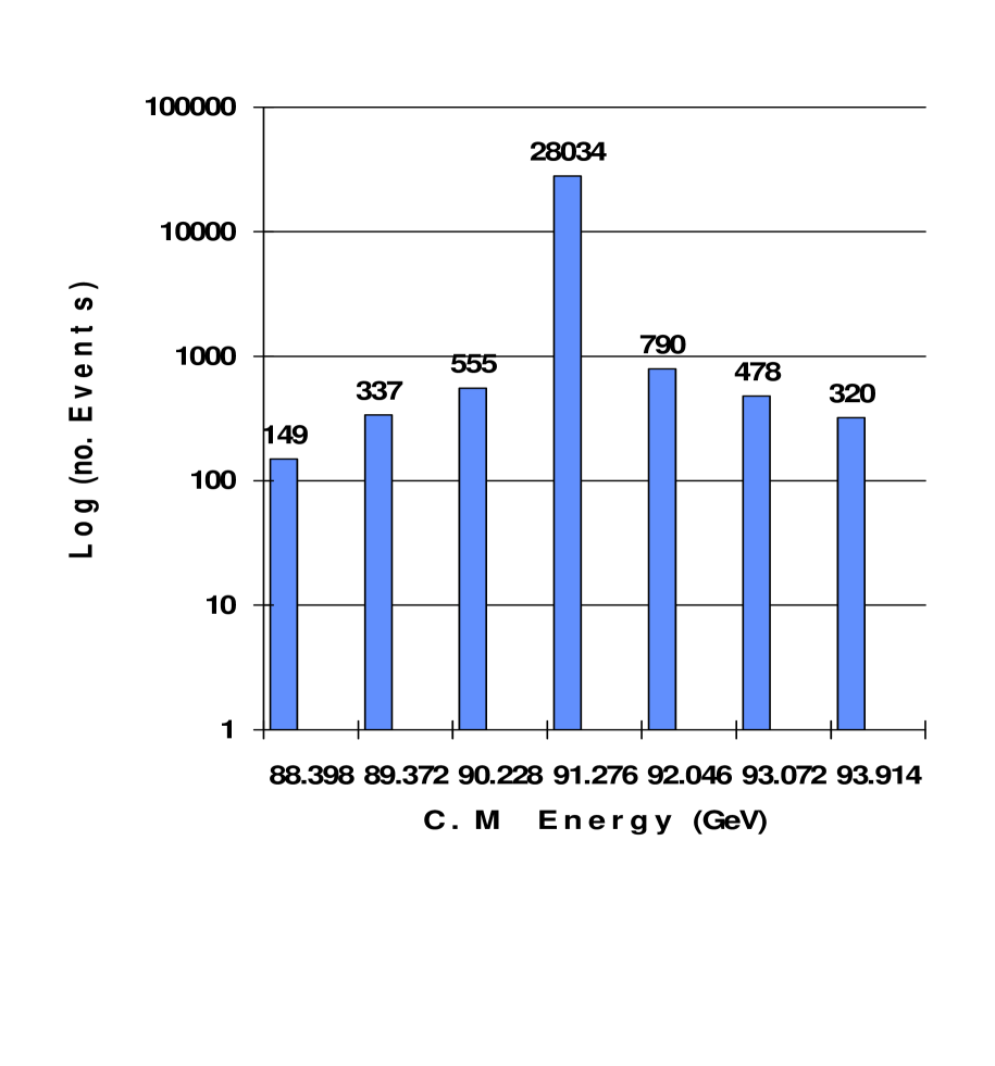
Figure 5.5: A logarithmic plot of the $E_{cm}$ distribution of the $\tau$-pairs selected in 1990-92. The numbers on top of each bin present the exact number of events. Most of the events (91.5%) are at the central energy bin (the Z⁰ peak).

Details of the background in each $\tau$-decay channel are discussed in the following chapters. Note that the criteria designed to remove two-photon (T4), Bhabha (T5) and mu-pair (T6) events introduce kinematic biases which must be studied for the measurement of the polarization. The treatment of the above selection criteria and the systematic uncertainties associated with them are considered in Chapter 6.

5.4 Tau Decay Identification

After selecting a $\tau$-pair event, an attempt is made to classify the $\tau$ decay channels of its two jets. Our $\tau$$\rightarrow$e$\bar{\nu}_{e}$$\nu_{\tau}$ identification algorithm selects jets containing a track which deposits almost all of its energy within a highly localized region of the ECAL. The $\tau$$\rightarrow$$\mu$$\bar{\nu}_{\mu}$$\nu_{\tau}$ selection requires an isolated charged track with energy deposition in the ECAL and HCAL consistent with the passage of a minimum-ionizing particle and signals in the MUON chambers associated with the track.

Unfortunately, the signature for a $\tau$$\rightarrow$$\pi$(K)$\nu_{\tau}$ decay is not as distinct as that for a $\tau$$\rightarrow$e$\bar{\nu}_{e}$$\nu_{\tau}$ or a $\tau$$\rightarrow$$\mu$$\bar{\nu}_{\mu}$$\nu_{\tau}$ decay because hadronic interactions may begin in the magnet coil, ECAL or HCAL. While electrons and muons can be efficiently removed from the $\tau$$\rightarrow$$\pi$(K)$\nu_{\tau}$ sample, the semi-leptonic tau decays containing neutral pions are problematic because at E_cm=91 $GeV$ the boost of the tau causes significant overlap in the ECAL of the charged pion hadronic shower and the electromagnetic showers from the $\pi^{0}$ decay to photons. We exploit the fact that electromagnetic interactions begin in the coil with a higher probability than hadronic interactions. The presampler thereby provides an effective veto against decays containing neutral pions.

5.4.1 $\tau$$\rightarrow$e$\bar{\nu}_{e}$$\nu_{\tau}$  identification

Typical candidate for the $\tau$$\rightarrow$e$\bar{\nu}_{e}$$\nu_{\tau}$ decays is characterized by a single track which deposits its energy in a narrow cone before the end of the ECAL. A tau jet is identified as a $\tau$$\rightarrow$e$\bar{\nu}_{e}$$\nu_{\tau}$ candidate if each of the following requirements are met.

E1.

The jet has one or two good charged tracks. If the jet has two tracks, the higher momentum track is taken as the electron candidate.

E2.

The ECAL energy associated to the candidate track divided by the track momentum, E/p, is between 0.7 and 2.

E3.

The electrons shower is expected not to be too wide. Hence, it is required that at least $90\%$ of the energy of the ECAL cluster associated with the candidate track is deposited within three lead-glass blocks.

E4.

The ECAL energy not associated to the candidate track, E_excess, is less than 4% of the beam energy. This removes tau decays containing neutral pions and highly radiative tau pair events.

E5.

The difference between the track and the presampler signal furthest away in $\phi$ but still assigned to the jet, $\delta\phi_{max}$, is less than $5^{\circ}$. This effectively removes tau decays containing neutral pions.

E6.

To reduce background coming from muons or from $\tau$ hadronic decays, the number of HCAL layers containing a signal which are assigned to the jet is less than two.

E7.

If the opposite tau jet contains a single charged track with a momentum greater than $75\%$ of the beam energy then the acoplanarity between the two jets must be greater than $0.1^{\circ}$. The acoplanarity is defined in the r-$\phi$ plane. This suppresses residual background from Bhabha events where one of the two electron energies is mismeasured.

E8.

The variable used for the polarization study of $\tau$$\rightarrow$e$\bar{\nu}_{e}$$\nu_{\tau}$ decays is the total electromagnetic energy associated with the jet divided by the beam energy, $x_{e}=E_{cls}/\mbox{$E_{beam}$}$. $E_{cls}$ is corrected for the energy lost in the material in front of ECAL where the correction uses presampler information. The $x$-parameter used in the fit is expected to be between 0 and 1. It can exceed 1 due to finite detector resolution. Values far above 1 might happen due to bad track reconstruction which is not fully taken into account in our parametrization of the resolution (see Sect. 6.3). Tau candidates with very high $x$ are few, but still may affect the result of the ML fit because of their extremely low probability. In order to restrict ourselves to a kinematic region with high and well understood electron identification efficiency, we require measured $x_{e}$ to be above 0.05 and below 1.1.

E9.

Fiducial requirements are imposed to remove candidates entering ECAL regions where the four subassemblies of the calorimeter come in contact. Good EB performance is important not only for the measurement of the electron energy, but also for electron pion identification using E/p cuts, and for Bhabha events rejection. The small gaps in the calorimeter coverage in these contact regions allow some Bhabha events to be accepted as $\tau$$\rightarrow$e$\bar{\nu}_{e}$$\nu_{\tau}$ candidates. Hence, a candidate is also removed if the track in the opposite jet points to one of these regions.

The PB subdetector is extremely important for the pion identification, but it is used also to correct the electron energy (see below in Sect. 6.3). If the track enters a region of the presampler which is not fully operational, the tau jet is also removed.

E10.

The jet is not identified as a $\tau$$\rightarrow$$\pi$(K)$\nu_{\tau}$ candidate according to the criteria listed below.

5.4.2 $\tau$$\rightarrow$$\mu$$\bar{\nu}_{\mu}$$\nu_{\tau}$  identification

The signature of this decay is an isolated charged track characterized by a small energy deposition in the ECAL and HCAL, and with associated signals in the MUON chambers, consistent with a passage of a minimum-ionizing particle. The $\tau$$\rightarrow$$\mu$$\bar{\nu}_{\mu}$$\nu_{\tau}$ candidate jet must satisfy each of the following requirements.

M1.

There is exactly one good charged track in the tau jet.

M2.

At least two of the following three criteria which characterize the passage of minimum ionizing particle must be met:

($i$) two or more hits in the MUON chambers are associated to the track,

($ii$) the number of HCAL layers containing associated hits, N${}^{HC}_{layers}$, is greater than three and N${}^{HC}_{hits/layer}$ is less than two,

($iii$) the ECAL energy in the jet is less than 2 $GeV$.

M3.

In order to further ensure the minimum ionizing particle characteristic, the jet is discarded if N${}^{HC}_{layers}$ is greater than two and N${}^{HC}_{hits/layer}$ is greater than or equal to three.

M4.

The combined invariant mass of the track (assuming a charged pion) and all the ECAL clusters in the jet (assuming $\gamma$) is less than 0.3 $GeV$. This is calculated after subtracting 0.5 $GeV$ from the cluster nearest to the track in order to account for energy deposition from a minimum ionizing particle. This suppresses contamination from semi-leptonic tau decays accompanied by neutral pions.

M5.

Residual background from e⁺e^- $\rightarrow$$\mu^{+}$$\mu^{-}$ events is suppressed by rejecting jets in which the opposite jet is consistent with a muon, and the sum of track momenta and ECAL energies, excluding the expected energy deposition of 0.5 $GeV$, is greater than $80\%$ of the beam energy. The opposite jet is considered to be a muon if:

($i$) one of the first two conditions of cut M2 is satisfied,

or if,

($ii$) the track extrapolates to a region not fully covered by any of the HCAL or MUON chambers.

M6.

A cut on the variable $x_{\mu}$ used for the polarization study of $\tau$$\rightarrow$$\mu$$\bar{\nu}_{\mu}$$\nu_{\tau}$ events. It is defined as $x_{\mu}=(p_{trk}+E_{cls}-0.5)/\mbox{$E_{beam}$}$ where $p_{trk}+E_{cls}$ is the sum of track momentum and ECAL energies associated to the jet, and 0.5 $GeV$ is the expected energy deposition of the muon. As in the electron case (see cut E8) the muon candidate is required to have $x_{\mu}$ above 0.05 and below 1.1 in order to ensure a reliable and well understood identification efficiency.

M7.

An additional fiducial requirement is imposed to suppress background from $\mu$-pair events having tracks close to an anode or cathode wire plane of the jet chamber. This source of background is not well simulated. A cut rejecting muon tracks near the anode wire planes has been included in the 1990 analysis [7]. Later this cut was removed from the TP standard cuts because it was believed that the momentum resolution near the anode wires has been improved and the remaining deficiency is properly described in GOPAL. However, a recent study [62] has demonstrated that there is still a problem, near the anode wires and even near the cathode wires. Due to the deteriorated resolution in those regions, $\mu$-pair events which should have been rejected by the cuts T6 and M5, still infiltrate to our sample more than expected from the MC. Consequently, a candidate track that is within 0.5^∘ of an anode plane or within 0.3^∘ of a cathode plane is removed if both tau jets are identified as muons or if one jet is identified as a muon and the opposite tau jet is not identified at all.

M8.

The jet is not accepted as a $\tau$$\rightarrow$$\mu$$\bar{\nu}_{\mu}$$\nu_{\tau}$ candidate if it also satisfies the $\tau$$\rightarrow$$\pi$(K)$\nu_{\tau}$ criteria listed below.

5.4.3 $\tau$$\rightarrow$$\pi$(K)$\nu_{\tau}$  identification

The difficulty in the identification of this channel arises from the fact that its signature is not highly distinct from those of other channels, and in particular hadronic channels with neutral pions.

A $\tau$$\rightarrow$$\pi$(K)$\nu_{\tau}$  candidate must satisfy the following requirements.

P1.

There is exactly one good charged track in the jet.

P2.

The total cluster energy associated to the track is less than $80\%$ of the reconstructed track momentum. This removes electrons and other contaminants having large deposited energy in ECAL.

P3.

E_excess is less than $2\%$ of the beam energy, and $\delta\phi_{max}$ is below $0.5^{\circ}$. This rejects semi-leptonic tau decays containing a neutral pion using the same variables described in the $\tau$$\rightarrow$e$\bar{\nu}_{e}$$\nu_{\tau}$ selection criteria E4 and E5.

P4.

In order to suppress the contamination from $\tau$$\rightarrow$$\mu$$\bar{\nu}_{\mu}$$\nu_{\tau}$ decays, only tracks extrapolating to a geometrical region in which there is active MUON chamber coverage are selected. Furthermore, if a track extrapolates to a region where HCAL is active, the jet is rejected if

($i$) the number of layers hit out of the four MUON chamber layers and the last three HCAL layers, N${}^{HC/MU}_{layers}$, is more than two,

and or,

($ii$) $\mbox{\rm N${}^{HC/MU}_{layers}$}=2$ and N${}^{HC}_{hits/layer}$ is below 3. If the track extrapolates to a region which is not fully covered by HCAL then the jet is rejected if the number of hit MUON layers is greater than 2.

P5.

The variable used in the polarization study of $\tau$$\rightarrow$$\pi$(K)$\nu_{\tau}$ is $x_{h}=p_{trk}/\mbox{$E_{beam}$}$. For the same arguments given for the electron and muon (cuts E8 and M5) the pion candidate is required to have $0.05<x_{h}<1.1$. This ensures a reliable and well understood identification efficiency.

P6.

Fiducial requirements are imposed to remove candidates entering ECAL regions where the eight subassemblies of the calorimeter come in contact (See E9). Tau jets are also removed if the track enters a region of the presampler which is not fully operational.

5.4.4 $\tau$$\rightarrow$$\rho$$\nu_{\tau}$  identification

The $\tau$$\rightarrow$$\rho$$\nu_{\tau}$ channel is not included in the present analysis. We utilize however, the results obtained by OPAL in other analyses (see Ref. [15] and  [14]) to combine with our findings. Hence, here we describe only briefly its selection procedure. Due to the fact the $\rho$ decays into a charged pion and a neutral pion, the signature of the $\tau$$\rightarrow$$\rho$$\nu_{\tau}$ decay is a single charged track accompanied by ECAL energy deposition consistent with the interaction of the two photons from the neutral pion decay.

Two analysis methods to identify rho decays were used in OPAL. The two $\tau$$\rightarrow$$\rho$$\nu_{\tau}$ identification algorithms (for Sample I and II) are similar to those used to measure the $\tau$$\rightarrow$h $\pi^{0}$ branching ratio [63]. The selection of sample I [14] is based on an attempt to reconstruct from the ECAL clusters the neutral pion which is then combined with the charged track to form a $\rho$-meson candidate.

The second $\tau$$\rightarrow$$\rho$$\nu_{\tau}$ selection procedure [15] uses a different $\pi^{0}$ identification algorithm. It finds clusters of activity in the ECAL which are restricted to a maximum size of 2$\times$2 blocks in $\theta$ and $\phi$ plane. Such clusters contain 99% of the energy of an electromagnetic shower and 95% of the energy of a hadronic shower. These clusters which are limited in size differ from those used in the $\tau^{+}$$\tau^{-}$selection or the $\tau$$\rightarrow$e$\bar{\nu}_{e}$$\nu_{\tau}$, $\tau$$\rightarrow$$\mu$$\bar{\nu}_{\mu}$$\nu_{\tau}$ and $\tau$$\rightarrow$$\pi$(K)$\nu_{\tau}$ identifications. Unlike the sample I selection, this algorithm accepts as $\pi^{0}$ candidates single clusters which are not associated to the track.

5.4.5 Summary of $\tau$ Decay Identification

The typical global efficiencies obtained by the selections described above are 65.8%, 72.1% and 30.4% for the $\tau$$\rightarrow$e$\bar{\nu}_{e}$$\nu_{\tau}$, $\tau$$\rightarrow$$\mu$$\bar{\nu}_{\mu}$$\nu_{\tau}$ and $\tau$$\rightarrow$$\pi$(K)$\nu_{\tau}$ , respectively. These numbers include the approximately 93% preselection efficiency within the fiducial region of the analysis and ignore decay or detection correlations. The corresponding background levels are 5.0%, 2.5% and 7.2%, respectively. Plots of the global efficiencies as a function of $x$ are shown in Fig. 5.6.

.

Figure 5.6: Global efficiencies as a function of $x$ for a) $\tau$$\rightarrow$e$\bar{\nu}_{e}$$\nu_{\tau}$b) $\tau$$\rightarrow$$\mu$$\bar{\nu}_{\mu}$$\nu_{\tau}$and c) $\tau$$\rightarrow$$\pi$(K)$\nu_{\tau}$ decays. The efficiencies include the 93% tau-pair selection efficiency and are after the fiducial cut of $|\cos\theta|<0.68$. The complex behavior in the low and high $x$ regions of a) and b) are caused by requirements designed to remove two-photon, Bhabha and mu-pair events.

The results from the $\tau$$\rightarrow$$\rho$$\nu_{\tau}$ decay are based on two samples of $\tau$$\rightarrow$$\rho$$\nu_{\tau}$ candidate events. Each sample is independently selected and values for $\langle P_{\tau}\rangle$ and A${}_{pol}^{FB}$ are determined separately. Both selections have an efficiency of approximately 50% and about one third of the combined number of candidates is common to both samples. Sample II candidates are selected only from the 1991 and 1992 data which contain 27353 tau-pair events. The efficiency for selecting sample I is 47.5% where the background is 21.2%. For sample II the efficiency is 57.5% and the background 22.5%.

In Table 5.2 we list the number of $\tau$-pair events in the data, according to their $\tau$ decay mode identifications. The percentage efficiencies and background are also presented for each event classification within $|\cos\theta|<0.68$. The efficiencies include the contributions from the tau-pair selection. The label ‘0’ refers to the case where the $\tau$ decay was not identified at all. The events in which none of the two jets was identified (23% of the whole sample) are not used in the analysis. As is evident from this table, the identification efficiencies of tau jets are not independent. The requirements that remove two-photon, Bhabha and mu-pair events introduce these correlations. Such correlations are, however, taken into account in the analysis.

Fig. 5.7 shows a ”typical” $\tau^{+}$$\tau^{-}$ selected event in the detector. In the figure we see an $e^{+}e^{-}\to\mbox{$\tau$}^{+}\mbox{$\tau$}^{-}$ event selected by our criteria. One of the tau decays into a one charged particle while on its back side we find a collimated 3 charged particles jet.

$\tau_{1}$ decay	$\downarrow$
No.	0	6833
No.	e	3585	574
$\epsilon$		54. (19.)	46.
$\beta$		5.	12.
No.	$\mu$	3897	1288	487
$\epsilon$		58. (23.)	58.	46.
$\beta$		3.	6.	5.
No.	$\pi(K)$	1145	346	385	55
$\epsilon$		26. (9.)	21.	25.	11.
$\beta$		7.	11.	8.	14.
No.	$\rho$	5879	1960	1985	623	1621
$\epsilon$		51. (19.)	44.	51.	20.	41.
$\beta$		27.	31.	29.	32.	48.
$\tau_{2}$ decay	$\rightarrow$	0	e	$\mu$	$\pi(K)$	$\rho$

Table 5.2: Classification of the $\tau$-pair events with $\mbox{$|\cos\theta|$}<0.68$ where the first figure in each box represent their number. The efficiency ($\epsilon$) and background ($\beta$) given in percentages are presented underneath. The efficiencies include the contributions from the tau-pair selection $\sim 93\%$. The efficiencies in the first column (i.e. when only one tau is identified) are subdivided into two classes: the first is for the case where the opposite tau does not decay into one of the four channels; the second (in brackets) is where the opposite tau decays into one of the four channels but is not identified. The label ‘0’ refers to the case where the $\tau$ decay was not identified.

.

Figure 5.7: A display of typical $\tau^{+}$$\tau^{-}$ event in the OPAL detector. Tracks in the central tracking system are shown in red. Small magenta boxes show hits in the TOF system. Clusters of energy in the lead glass ECAL are shown as blue boxes, of size proportional to their energy. Similarly, clusters of energy in the HCAL are drawn in green. Penetrating charged particle tracks, which are candidates for muons, are shown as light-blue arrows. In this event ,one of the taus (on the right side) has decayed to a penetrating muon, and the other to an electron.

Chapter 6 Physics Analysis

6.1 The Fit Procedure

For the analysis of the $\tau$$\rightarrow$e$\bar{\nu}_{e}$$\nu_{\tau}$, $\tau$$\rightarrow$$\mu$$\bar{\nu}_{\mu}$$\nu_{\tau}$ and $\tau$$\rightarrow$$\pi$(K)$\nu_{\tau}$ decays, $\langle P_{\tau}\rangle$  and A${}_{pol}^{FB}$ are determined using an event-by-event ML fit to the data of the theoretical distribution (Eq. 4.37). In this method, the following expression is minimized,

$$W=-2\ln{\cal L}=-2\sum_{n=1}^{N}\ln\left\{\frac{1}{\mbox{$\mbox{$\sigma^{\mbox{\small$\prime$}}$}_{ij}$}}\frac{d^{3}\mbox{$\mbox{$\sigma^{\mbox{\small$\prime$}}$}_{ij}$}}{d\mbox{$\cos\theta$}\>d\mbox{$x_{i}$}\>d\mbox{$x_{j}$}}\right\}_{n},$$ (6.1)

where ${\cal L}$ is the likelihood function. The sum in Eq. 6.1 runs over all $N$ selected $\tau$-pair events, where at least one of the two $\tau$’s has been identified as a $\tau$$\rightarrow$e$\bar{\nu}_{e}$$\nu_{\tau}$, $\tau$$\rightarrow$$\mu$$\bar{\nu}_{\mu}$$\nu_{\tau}$ or $\tau$$\rightarrow$$\pi$(K)$\nu_{\tau}$ candidate. The term in the logarithm is the differential cross-section for a production $\tau$-pairs where one $\tau$ decays into channel $i$ and the second one decays into channel $j$ ( Eq. 4.37). It is normalized to one, and corrected for radiation, $x$ resolution, efficiency and background effects, hence it will be denoted as primed $\sigma$. This term corresponds to the case where both $\tau$ decays are identified. When only one decay is identified, it must be replaced by $(1/\mbox{$\mbox{$\sigma^{\mbox{\small$\prime$}}$}_{i}$})d^{2}\mbox{$\mbox{$\sigma^{\mbox{\small$\prime$}}$}_{i}$}/d\mbox{$\cos\theta$}\;d\mbox{$x_{i}$}$.

When both $\tau$ decays are identified, the corrected cross-section can be written in the following form,

$$\frac{16}{3}\frac{1}{\mbox{$\mbox{$\sigma^{\mbox{\small$\prime$}}$}_{ij}$}}\frac{d^{3}\mbox{$\mbox{$\sigma^{\mbox{\small$\prime$}}$}_{ij}$}}{d\mbox{$\cos\theta$}\>d\mbox{$x_{i}$}\>d\mbox{$x_{j}$}} = \sum_{hel=\pm}\{[(1\pm\mbox{$\langle P_{\tau}\rangle$})(1+\mbox{$\cos^{2}\theta$})+\mbox{$\frac{8}{3}$}(\mbox{\rm A${}_{FB}$}\pm\mbox{\rm A${}_{pol}^{FB}$})\mbox{$\cos\theta$}]$$ (6.2)

$$\times \mbox{${\cal E}^{\pm}_{ij}(\mbox{$x_{i}$},\mbox{$x_{j}$},\mbox{$\cos\theta$})$}[\mbox{$h^{\pm}_{i}(\mbox{$x_{i}$})$}\mbox{$\epsilon_{i}(\mbox{$x_{i}$},\mbox{$\cos\theta$})$}+\mbox{$\beta^{\pm}_{i}(\mbox{$x_{i}$},\mbox{$\cos\theta$})$}]$$

$$\times [\mbox{$h^{\pm}_{j}(\mbox{$x_{j}$})$}\mbox{$\epsilon_{j}(\mbox{$x_{j}$},\mbox{$\cos\theta$})$}+\mbox{$\beta^{\pm}_{j}(\mbox{$x_{j}$},\mbox{$\cos\theta$})$}]\}$$

$$+ \mbox{$\beta^{non-\tau}_{ij}(\mbox{$x_{i}$},\mbox{$x_{j}$},\mbox{$\cos\theta$})$}.$$

Here ${\cal E}^{\pm}_{ij}(\mbox{$x_{i}$},\mbox{$x_{j}$},\mbox{$\cos\theta$})$ is the efficiency for selecting a $\tau$-pair event in which one tau decays via channel $i$ and the other via $j$, $\epsilon_{i}(\mbox{$x_{i}$},\mbox{$\cos\theta$})$ is the efficiency for identifying channel $i$ which for some of the decay combinations depends on the decay mode in the opposite jet and on the helicity. The $\beta^{\pm}_{i}(\mbox{$x_{i}$},\mbox{$\cos\theta$})$ is the distribution of background events from other $\tau$ decay channels when applying the channel $i$ selection procedure and $\beta^{non-\tau}_{ij}(\mbox{$x_{i}$},\mbox{$x_{j}$},\mbox{$\cos\theta$})$ corresponds to background contributions from events which are not tau-pairs. The function $h^{\pm}_{i}(\mbox{$x_{i}$})$ is the $x$ distribution for channel $i$, after applying corrections for detector resolution and radiative effects to $f_{i}(x_{i})\pm g_{i}(x_{i})$. It is given by the following convolution function

$$\mbox{$h^{\pm}_{i}(\mbox{$x_{i}$})$}=C_{i}\int_{0}^{1}[\mbox{$f_{i}$}(\mbox{$x_{i}$}^{0})\pm\mbox{$g_{i}$}(\mbox{$x_{i}$}^{0})]\mbox{$r^{\pm}_{i}(\mbox{$x_{i}$})$}\mbox{${\cal R}_{i}(\mbox{$x_{i}$}^{0},\mbox{$x_{i}$})$}d\mbox{$x_{i}$}^{0}.$$ (6.3)

where the normalization factor $C_{i}$ was introduced to satisfy,

$$\int_{0}^{\infty}\mbox{$h^{\pm}_{i}(\mbox{$x_{i}$})$}d\mbox{$x_{i}$}=1.$$ (6.4)

The $\mbox{$x_{i}$}^{0}$ is the $x_{i}$ before resolution effects are taken into account. The functions $f_{i}$ and $g_{i}$ are the Born distributions listed in Chapter  4, Eqs. 4.30, 4.33, 4.35, 4.36. The correction term $r^{\pm}_{i}(\mbox{$x_{i}$})$ is due to radiative effects and ${\cal R}_{i}(\mbox{$x_{i}$}^{0},\mbox{$x_{i}$})$ is the momentum resolution function.

If only one tau decay is identified, the corrected differential cross-section takes a simpler form,

$$\frac{16}{3}\frac{1}{\mbox{$\mbox{$\sigma^{\mbox{\small$\prime$}}$}_{i}$}}\frac{d^{2}\mbox{$\mbox{$\sigma^{\mbox{\small$\prime$}}$}_{i}$}}{d\mbox{$\cos\theta$}\>d\mbox{$x_{i}$}} = \sum_{hel=\pm}\{[(1\pm\mbox{$\langle P_{\tau}\rangle$})(1+\mbox{$\cos^{2}\theta$})+\mbox{$\frac{8}{3}$}(\mbox{\rm A${}_{FB}$}\pm\mbox{\rm A${}_{pol}^{FB}$})\mbox{$\cos\theta$}]$$ (6.5)

$$\times {\cal E}^{\mbox{\small$\prime$}\pm}_{i}(\mbox{$x_{i}$},\mbox{$\cos\theta$})[\mbox{$h^{\pm}_{i}(\mbox{$x_{i}$})$}\mbox{$\epsilon_{i}(\mbox{$x_{i}$},\mbox{$\cos\theta$})$}+\mbox{$\beta^{\pm}_{i}(\mbox{$x_{i}$},\mbox{$\cos\theta$})$}]\}$$

$$+ \mbox{$\beta^{non-\tau}_{ij}(\mbox{$x_{i}$},\mbox{$x_{j}$},\mbox{$\cos\theta$})$},$$

where ${\cal E}^{\mbox{\small$\prime$}\pm}_{i}(\mbox{$x_{i}$},\mbox{$\cos\theta$})$ is given by the following expression,

$${\cal E}^{\mbox{\small$\prime$}\pm}_{i}(\mbox{$x_{i}$},\mbox{$\cos\theta$}) = {\cal E}^{\pm}_{i}(\mbox{$x_{i}$},\mbox{$\cos\theta$})$$

$$+ \frac{1}{1-\sum_{j}B_{j}}\sum_{j\neq i}B_{j}\int d\mbox{$x_{j}$}\mbox{${\cal E}^{\pm}_{ij}(\mbox{$x_{i}$},\mbox{$x_{j}$},\mbox{$\cos\theta$})$}\mbox{$h^{\pm}_{j}(\mbox{$x_{j}$})$}[1-\mbox{$\epsilon_{j}(\mbox{$x_{j}$},\mbox{$\cos\theta$})$}].$$

Here, the first term is the efficiency for selecting a $\tau$-pair event in which one tau decays via channel $i$ and the other via a channel not included in our analysis. The second term is the contribution of events where the other channel is included in our analysis but is not identified due to inefficiency. The coefficients $B_{j}$ are the $\tau$ branching fractions. They were taken from the OPAL measurements [7]. The summation in Eq. 6.1 is over the three decay channels considered in this analysis.

The normalization factor in Eq. 6.1, $\mbox{$\sigma^{\mbox{\small$\prime$}}$}_{ij}$ (or $\mbox{$\sigma^{\mbox{\small$\prime$}}$}_{i}$ in the case of only one identified tau) are the total corrected cross sections evaluated in every step of the fitting procedure.

Our fitted parameters are $\langle P_{\tau}\rangle$ and A${}_{pol}^{FB}$. In a former work of OPAL [6] the values of A_FB($s$) have been determined using the distribution of $\cos\theta$ alone. In the present analysis we have used these reported values as an input. Since A_FB has a strong $s$ dependence (see Fig. 4.9), we divide the available c.m. energy range as shown in Fig. 5.5 into 7 intervals. For each interval we calculate the average of the OPAL A_FB measurements taken during 1989-1992. In our global fit we use for each event the corresponding A_FB value according to its c.m. energy. The energy intervals, the average energies, the sample sizes and the corresponding A_FB values are listed in Table 6.1. The uncertainties in the A_FB values were taken into account in the calculation of the overall systematic error.

$E_{cm}$	$\langle\mbox{$E_{cm}$}\rangle$	# of	AFB
($GeV$)	($GeV$)	events	(%)
87.7 - 88.7	88.398	149	$-29.0\pm 5.1$
88.7 - 89.7	89.372	337	$-8.4\pm 4.0$
89.7 - 90.7	90.228	555	$-7.8\pm 3.2$
90.7 - 91.7	91.276	28034	$1.2\pm 0.5$
91.7 - 92.7	92.046	790	$5.1\pm 2.8$
92.7 - 93.7	93.072	478	$10.8\pm 3.4$
93.7 - 94.7	93.914	320	$14.6\pm 4.0$

Table 6.1: Forward-backward asymmetries used in the fit and numbers of events for 7 c.m. energy intervals.

In performing the fit, the functions $h^{\pm}_{i(j)}$, $\epsilon_{i(j)}$, $\beta^{\pm}_{i(j)}$, ${\cal E}^{\pm}_{i(ij)}$ and $\beta^{non-\mbox{$\tau$}}_{i(ij)}$ as well as the normalization factors are calculated for each event. The $h^{\pm}_{i(j)}$ functions are obtained from the theoretical decay spectra corrected for radiative effects using large MC $\tau^{+}$$\tau^{-}$ event samples generated without detector simulation and corrected for resolution effects using resolution functions measured in data samples of e⁺e^- $\rightarrow$e⁺e^- events, low energy “single electron” events from highly radiative Bhabha scattering, and  e⁺e^- $\rightarrow$$\mu^{+}$$\mu^{-}$ events. The $\epsilon_{i(j)}$, ${\cal E}^{\pm}_{i(ij)}$, $\beta^{\pm}_{i(j)}$ and $\beta^{non-\mbox{$\tau$}}_{i(ij)}$ functions are parametrized in terms of simple functions, in most cases low order polynomials, using few parameters. The parameters are determined from fits to the pertinent MC samples and subsequently corrected using appropriate control samples from the data. The uncertainties in the parameters, their correlations and the corrections are taken into account in the treatment of systematic errors which are discussed in detail below. For this we are using the standard error propagation rule,

$$\Delta A=\sqrt{\sum_{i,j}\frac{\partial A}{\partial p_{i}}\frac{\partial A}{\partial p_{j}}\Delta p_{i}\Delta p_{j}\rho_{ij}}\;\;,$$ (6.7)

where $A$ is the final result ($\langle P_{\tau}\rangle$ or A${}_{pol}^{FB}$), $p_{i}$, $p_{j}$ are the parameters used to describe the correction function and $\rho_{ij}$ is the correlation matrix between them. The partial derivatives $\frac{\partial A}{\partial p_{i}}$ are calculated numerically, by modifying the parameter by its uncertainty, by repeating our fit and calculating the change in the final result $A$.

As suggested in Sect. 4.3 in order to check the parameters characterizing the structure of the charged weak decay of the $\tau$ one has also to treat them as free parameters. In that case we use Eqs. 4.3 and  4.48 to modify Eq. 6.2 in the following way:

$$\frac{d^{3}\mbox{$\mbox{$\sigma^{\mbox{\small$\prime$}}$}_{ij}$}}{d\mbox{$\cos\theta$}\>d\mbox{$x_{i}$}\>d\mbox{$x_{j}$}} =\frac{3\sigma}{64}\times\{ \;\;h^{+}_{i}h^{+}_{j}[{\cal C}(1+\xi_{i}\xi_{j})-{\cal P}(\xi_{i}+\xi_{j})]$$

$$+h^{-}_{i}h^{-}_{j}[{\cal C}(1+\xi_{i}\xi_{j})+{\cal P}(\xi_{i}+\xi_{j})]$$

$$+h^{+}_{i}h^{-}_{j}[{\cal C}(1-\xi_{i}\xi_{j})-{\cal P}(\xi_{i}-\xi_{j})]$$

$$+h^{+}_{i}h^{-}_{j}[{\cal C}(1-\xi_{i}\xi_{j})+{\cal P}(\xi_{i}-\xi_{j})]$$

$$+2(\rho-0.75) \;\;[f^{i}_{2}(\phi^{j}_{+}({\cal C}-{\cal P})+\phi^{j}_{-}({\cal C}+{\cal P})$$

$$+f^{j}_{2}(\phi^{i}_{+}({\cal C}-{\cal P})+\phi^{i}_{-}({\cal C}+{\cal P})]$$

$$+2(\delta-0.75) \;\;[\xi_{i}g^{i}_{2}(\phi^{j}_{+}({\cal C}-{\cal P})-\phi^{j}_{-}({\cal C}+{\cal P})$$

$$+\xi_{j}g^{j}_{2}(\phi^{i}_{+}({\cal C}-{\cal P})-\phi^{i}_{-}({\cal C}+{\cal P})]\}$$

where $\cal C,\cal P$, $h^{\pm}_{i(j)}$ and $\phi_{i(j)}^{\pm}$ are defined as following:

$${\cal C} = 1+\mbox{$\cos^{2}\theta$}+\mbox{$\frac{8}{3}$}\mbox{\rm A${}_{FB}$}\mbox{$\cos\theta$}$$

$${\cal P} = \mbox{$\langle P_{\tau}\rangle$}(1+\mbox{$\cos^{2}\theta$})+\mbox{$\frac{8}{3}$}\mbox{\rm A${}_{pol}^{FB}$}\mbox{$\cos\theta$}$$

$$h^{\pm}_{i} = f^{i}_{1}(\mbox{$x_{i}$})+\frac{3}{4}f^{i}_{2}(\mbox{$x_{i}$})\pm[g^{i}_{1}(\mbox{$x_{i}$})+\frac{3}{4}g^{i}_{2}(\mbox{$x_{i}$})]$$ (6.9)

$$\phi^{i}_{\pm} = f^{i}_{1}(\mbox{$x_{i}$})+\rho f^{i}_{2}(\mbox{$x_{i}$})\pm\xi_{i}[g^{i}_{1}(\mbox{$x_{i}$})+\delta g^{i}_{2}(\mbox{$x_{i}$})]$$

In the first two terms of Eq. 6.1 (first two lines) there is an exact repetition on Eq. 4.37 where a $V-A$ structure is assumed for the $\tau$ decay. These terms are corrected for radiation and detector (resolution, efficiency and purity) effects as in Eq. 6.2. For the other six terms, which vanish in the case when $V-A$ is exact, we cannot use the standard correction procedure as our calculated correction are helicity dependent. Therefore in order to correct these terms we used corrections averaged over the two helicity states. For example, $r_{i}(\mbox{$x_{i}$})=0.5\cdot[r_{i}^{+}(\mbox{$x_{i}$})+r_{i}^{-}(\mbox{$x_{i}$})]$.

Eqs. 6.1 and 6.1 as it is written is applicable to the $\tau$$\rightarrow$$\ell$$\bar{\nu}_{\ell}$$\nu_{\tau}$ events through which $\xi,\rho$ and $\delta$. In the case of $\tau$$\rightarrow$$\pi$(K)$\nu_{\tau}$ decay only $\xi_{had}$ can be measured. In order to generalize Eq. 6.1 and 6.1 we equate for the hadronic decays $f(g)^{had}=f(g)^{had}_{1}+f(g)^{had}_{2}$ where their values, not to change Eq. 4.33 relations, are:

$$f^{had}_{2} = 0$$

$$g^{had}_{2} = 0$$

$$f^{had}_{1} = \frac{1}{1-\mbox{$m_{h}^{2}$}/\mbox{$m_{\tau}^{2}$}}$$ (6.10)

$$g^{had}_{1} = \frac{2x-1-\mbox{$m_{h}^{2}$}/\mbox{$m_{\tau}^{2}$}}{(1-\mbox{$m_{h}^{2}$}/\mbox{$m_{\tau}^{2}$})^{2}}$$

6.2 Radiative and Threshold Effects

For a given helicity state, initial and final state radiation as well as radiation in the decay of the tau affect the spectra of the tau decay products. The radiative distortions to the spectrum for the decay mode $i$ are taken into account using a radiative correction function, $r^{\pm}_{i}(\mbox{$x_{i}$})$.

Radiative effects are usually separated into photonic (QED) and weak interaction effects. The QED effects are due to all the diagrams involving real or virtual photons. They do not depend on unknown parameters but they usually depend on the experimental cuts. The other effects are due to the weak corrections and depend on unknown theoretical parameters but not on the experimental cuts.

Since the $\tau$-polarization results are part of the Z⁰ OPAL lineshape parameters and are used with them in all sorts of overall electroweak fits, they are handled in the same way. Therefore, following the procedure used in all LEP experiments for the line shape analysis, we do not apply corrections due to QED and weak radiative effects on the measured $\langle P_{\tau}\rangle$ or A${}_{pol}^{FB}$. However, even for a given helicity state, initial and final state radiation modify the spectrum of outgoing leptons and pions.

The functions $r^{\pm}_{i}(\mbox{$x_{i}$})$ are determined from the ratio of the spectrum containing radiative effects to the spectrum where only the Born level cross-section is considered. A high statistics run of the KORALZ 4.0 MC generator, is used to create the radiative corrected spectrum.

The QED effects, and in particular the initial state radiation, depend on the c.m. energy. We use in this analysis data taken on the Z⁰ peak as well as at 1, 2 and 3  $GeV$ below and above the peak (see Table 6.1). Therefore the KORALZ 4.0 is used to generate events distributed at the same seven c.m. energies as in the data. We actually generated three samples of 420000 events each, corresponding to the three decay channels investigated here. In each sample, all the $\tau$’s were forced to decay into a single channel.

For the $\tau$-polarization measurement on the Z⁰ , the most important QED effect is the final state radiation from the $\tau$ or its decay products [4] . This would modify the decayed particle momentum and distort its distribution from the Born term expectation. In order to minimize this effect in our analysis, the electromagnetic calorimeter is used to detect the radiated photons in a $35^{\circ}$ cone around the track. The energy of these photons is added to the track energy and in this way, the effect of the final state radiation is minimized. This procedure is done only for lepton final states, since in the case of pions, events with extra photons are rejected anyhow, because they resemble $\tau$$\rightarrow$$\rho$$\nu_{\tau}$ decays. The same treatment is done also for the generated events in order to investigate the residual effect of radiative corrections.

.

Figure 6.1: $x$ distribution of the ratio between generated MC events with radiative corrections and the Born term expectation, plotted with our parametrization for the radiative effects (solid lines). Figs. a) and b) are for the $\tau$$\rightarrow$e$\bar{\nu}_{e}$$\nu_{\tau}$ channel for positive and negative helicity states respectively. Figs. c) and d) correspond to the $\tau$$\rightarrow$$\mu$$\bar{\nu}_{\mu}$$\nu_{\tau}$ channel and Figs. e) and f) are for the $\tau$$\rightarrow$$\pi$(K)$\nu_{\tau}$ channel.

We calculated separately the radiative corrections, $r^{\pm}_{i}(\mbox{$x_{i}$})$, separately for positive and negative helicity events. In this way the corrections are independent on the polarization measurement. The MC distributions are divided by the corresponding lowest order diagram expectations. The obtained ratios are the radiative corrections $r^{\pm}_{i}(\mbox{$x_{i}$})$ which are plotted in Fig. 6.1. These are slightly dependent on the helicity state. The reason of this dependence originates partly from the different slopes of the Born spectra. For instance, in the channel $\tau$$\rightarrow$$\pi$(K)$\nu_{\tau}$ the spectrum is increasing (decreasing) for positive (negative) helicity. The initial and final state radiation tend to decrease the energy of the outgoing pion. Therefore, one should expect the low $x$ range be enhanced and distorts the distribution.

The solid lines in Fig. 6.1 represent our parametrization. We needed 3 to 4 parameters to describe each distributions. The $\chi^{2}$ values between the distributions and their parametrization are indicated in the figures. The first bin in Figs. 6.1c and 6.1d is low due to the finite $\mu$-mass effect, which will be discussed in the following, and was not incorporated in the Born expression. Therefore, this bin was not included in the $\chi^{2}$ calculation. For the $\tau$$\rightarrow$$\pi$(K)$\nu_{\tau}$ channel the first bin starts at the kinematical threshold and therefore no depletion is presented.

The major uncertainty associated with these corrections arises from the fact that the ${\cal O}(\alpha)$ in the QED corrections to tau decay are included only in the leading logarithmic approximation. The effect of this correction on the polarization asymmetries is quantified by analyzing the MC event sample after full simulation as if it was measured data. The event sample is analyzed twice, once for the full event sample and also for a sample which excludes events with radiated photons in the tau decay process. The difference in the results is used as a measure of the magnitude of the correction. Following Ref. [65], the correction is assumed to have a systematic error of the order of $1/\ln(\mbox{$m_{\tau}$}/m_{i})$ of the correction. An additional but small contribution to

the error on $r^{\pm}_{i}(\mbox{$x_{i}$})$ arises from the parameters used to describe the radiative corrections due to the MC statistics which is large but nevertheless limited. These parameters are obtained, together with their correlations, from the fits of the parametrization functions. Their effect on the final $\langle P_{\tau}\rangle$ and A${}_{pol}^{FB}$ results was calculated with the method described in the last section.

Table 6.2 summarizes the systematic errors associated with the radiative corrections for the various decay channels and for the whole sample.

	all		$\tau$$\rightarrow$e$\bar{\nu}_{e}$$\nu_{\tau}$		$\tau$$\rightarrow$$\mu$$\bar{\nu}_{\mu}$$\nu_{\tau}$		$\tau$$\rightarrow$$\pi$(K)$\nu_{\tau}$
source	$\Delta\langle P_{\tau}\rangle$	$\Delta$ A${}_{pol}^{FB}$	$\Delta\langle P_{\tau}\rangle$	$\Delta$ A${}_{pol}^{FB}$	$\Delta\langle P_{\tau}\rangle$	$\Delta$ A${}_{pol}^{FB}$	$\Delta\langle P_{\tau}\rangle$	$\Delta$ A${}_{pol}^{FB}$
MC	0.15	0.01	0.44	0.06	0.56	0.04	0.14	0.01
LL	0.25	0.03	0.16	0.03	0.15	0.04	0.33	0.02
Total	0.29	0.03	0.47	0.07	0.58	0.06	0.36	0.02

Table 6.2: Systematic errors (in %) associated with radiative effects. MC is the systematic error introduced by the MC finite statistics and LL is the main contribution coming from the leading logarithm approximation. Their quadratic sum is given in the last line.

As can be seen the treatment of initial and final state radiation in KORALZ 4.0 introduces a smaller contribution to the error than the leading logarithm approximation. The total error assigned to the radiative correction uncertainties of $\langle P_{\tau}\rangle$ and A${}_{pol}^{FB}$ are 0.29% and 0.03%.

We also investigated the possible influence of the radiative corrections on the $\cos\theta$ distributions. Since we found this to be negligible we have further taken $r^{\pm}_{i}(\mbox{$x_{i}$})$ to be independent of $\cos\theta$.

To account for the finite muon mass in the $\tau$$\rightarrow$$\mu$$\bar{\nu}_{\mu}$$\nu_{\tau}$ channel we have multiplied the expression under the integral of Eq. 6.3 by the term $K^{\pm}(x)$ defined as

$$K^{\pm}(x)=\left\{\begin{array}[]{ll}1-\left(\frac{x_{m}^{\pm}}{x}\right)^{q^{\pm}}&\mbox{for $x>x_{m}^{\pm}$}\\ 0&\mbox{for $x\leq x_{m}^{\pm}$}\end{array}\right.$$ (6.11)

The $x_{m}$ and $q$ parameters are given in Table 6.3. They were derived from a large MC event sample. Fig. 6.2 shows the $x$ distribution of these MC events at the low $x$ region together with our parametrization.

helicity	$x_{m}^{\pm}$	$q^{\pm}$
$(+)$	0.0024	1.27
$(-)$	0.0047	1.56

Table 6.3: Parametrization of the finite $\mu$-mass effect.

.

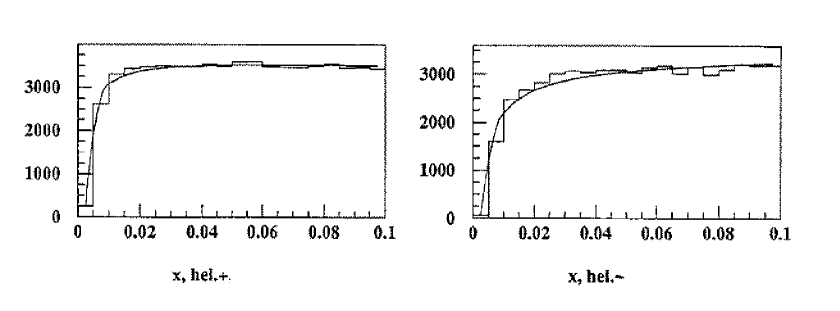
Figure 6.2: Low $x$ distributions of positive and negative helicity $\tau$$\rightarrow$$\mu$$\bar{\nu}_{\mu}$$\nu_{\tau}$ events obtained from high statistics MC sample (histograms), compared with our parametrization (solid line) of the finite $\mu$ mass effect.

The effect of the threshold for tau decays to kaons (Eq. 4.34) introduces an error on $\langle P_{\tau}\rangle$ and A${}_{pol}^{FB}$ associated with the uncertainties in the tau branching ratios to pions and kaons and leads to errors below 0.1%. There is also a very small error (less than 0.1%) introduced from the measurement uncertainty of A_FB [6]  which enters the analysis (see Eq. 4.27).

6.3 Detector Resolution

As in every experimental observation the measured quantities have a natural spread which depends on the detector resolution. The main influence of this in our analysis comes from the resolution in $x$ which is essential for the polarization measurement. We are less effected by the inaccuracy in the measurement of $\cos\theta$ since our fit to A${}_{pol}^{FB}$ is sensitive mainly to the numbers of forward and backward scattered particles and not to the specific shape of the $\cos\theta$-distribution. Our results are also not effected by the charge misassignment effect, which occurs only in a very small number of events.

A non-negligible effect on $\langle P_{\tau}\rangle$ and A${}_{pol}^{FB}$ can rise from the $x$-smearing, since the fit is sensitive to very small deviations from the true shape of the $x$-distribution. In particular, due to this smearing, some particles may have an unphysical $x$ value above one, which requires a special care.

To describe the resolution effect we introduce the $x$ resolution function, ${\cal R}_{i}(\mbox{$x_{i}$}^{0},\mbox{$x_{i}$})$, which is for a given $x^{0}$ the measured $x$. This function depends on the identification of the particle.

For pions, $x$ is the particle momentum normalized to the beam energy. For muons, we add to the particle momentum also the energy deposited in the EM calorimeter associated with the $\tau$-jet. From this EM energy we subtract 0.5  $GeV$, which is the expected energy deposited by the muon itself. This is done in order to include the energy of a photon which might be radiated from the tau or the muon. This correction is very small in most events, therefore, also for muons the resolution in $x$ is essentially the momentum resolution.

For electrons however, we are using only the EM calorimeter to define $x$, summing up all the clusters in the $\tau$-jet. Therefore, the resolution function for electrons is completely different than that of the $\mu$ or $\pi$. Both resolution

functions, for e, $\mu$ or $\pi$, are investigated in two steps. In the first step we determine a characteristic variable $y$, which takes into account the resolution dependence on $x$ and possibly also $\cos\theta$. In the second step we are using a control sample to investigate the exact shape of the $y$ distribution. In the following we shall discuss each resolution function separately.

6.3.1 The Resolution Function for Muons and Pions

First we examine only the shape of $\Delta x/x$ where as before $x=p_{track}/E_{beam}$ and $\Delta x$ is the difference between the true and measured normalized momentum, $\mbox{$x$}-x^{0}$, for each decay particle respectively. This was investigated by M. Sasaki [66] using $\tau$$\rightarrow$$\mu$$\bar{\nu}_{\mu}$$\nu_{\tau}$ and $\tau$$\rightarrow$$\pi$(K)$\nu_{\tau}$ MC events which were initially generated by KORALZ 3.8, and then processed by GOPAL129 and ROPE403. For this study a Gaussian distribution of the kind

$$P(\mbox{$x$},\bar{x})=\frac{1}{\sqrt{2\pi}\sigma(x)}e^{-\frac{(x-\bar{x})}{2\sigma^{2}(x)}}$$ (6.12)

was taken allowing also a possible shift in the average $\bar{x}$ parametrized as

$$\bar{x}=a_{1}+a_{2}x^{0}+a_{3}{(x^{0})}^{2}$$ (6.13)

The distribution of $\mbox{$x$}(x^{0})$ was investigated separately in 40 intervals between 0 to 1. Neglecting the non Gaussian tails the $\bar{x}$ shift and the width $\sigma(x)$ were determined for each $x$ interval. The relation between $\frac{\sigma(x)}{x}$ and the track momentum was taken to be

$$\frac{\sigma(x_{\pi})}{x_{\pi}}=\sqrt{b_{1}^{2}+b_{2}^{2}p_{track}^{2}}$$ (6.14)

and from this fitted values for $b_{1}$ and $b_{2}$ could be obtained (see Table 6.4). Fig. 6.3 illustrates the peak $(\bar{x}-x)$ shift and the Gaussian width as a function of $x_{\pi}^{0}$, together with the fitted curves estimated from the MC.

.

Figure 6.3: MC $\tau$$\rightarrow$$\pi$(K)$\nu_{\tau}$ resolution parametrization with the peak $(\bar{x}-x)$ shift (top) and the resolution $\sigma_{x}/x$ (bottom). The solid lines present the fit curves.

For the $\tau$$\rightarrow$$\mu$$\bar{\nu}_{\mu}$$\nu_{\tau}$ decays, $x_{\mu}$ has a more complicated definition, namely

$$\mbox{$x$}_{\mu}=\frac{p_{track}-E_{cls}-0.5~{}GeV}{E_{beam}}$$ (6.15)

where $\mbox{$x$}_{\mu}$ depends on both the $E_{cls}$ and the track momentum. Therefore the resolution function for the $\tau$$\rightarrow$$\mu$$\bar{\nu}_{\mu}$$\nu_{\tau}$ is a combination of the ECAL energy and the charged track momentum resolution. This combination introduces tuning parameters to weight the components assuming that this decay deposits the minimum ionizing energy of $0.5~{}GeV$ in the ECAL. Hence, the width term has the form

$$\sigma(\mbox{$x$}_{\mu})=\frac{\sqrt{b_{1}^{2}\cdot\sigma_{E_{cls}}^{2}+b_{2}^{2}\cdot\sigma^{2}_{ptrk}}}{E_{beam}}|_{E_{cls}=0.5\;GeV}$$ (6.16)

Fig. 6.4 illustrates $(\bar{x}-x)$ shift and the Gaussian width as a function of $x_{\mu}^{0}$, together with the fitted curves estimated from the MC.

.

Figure 6.4: MC $\tau$$\rightarrow$$\mu$$\bar{\nu}_{\mu}$$\nu_{\tau}$ resolution parametrization with the peak $(\bar{x}-x)$ shift (top) and the resolution $\sigma_{x}/x$ (bottom). The solid lines present the fit curves.

Table 6.4 presents the results of the fitted parameters. As can be seen, a shift in the peak appears only in the $\tau$$\rightarrow$$\mu$$\bar{\nu}_{\mu}$$\nu_{\tau}$ decays. This means that the energy of 0.5 $GeV$ assumed to be deposit by the muon in the ECAL was underestimated.

	$a_{1}$	$a_{2}$	$a_{3}$	$b_{1}$	$b_{2}$
$\tau$$\rightarrow$$\mu$$\bar{\nu}_{\mu}$$\nu_{\tau}$	0.0029	1.0000	0.0000	1.0610	1.1270
$\tau$$\rightarrow$$\pi$(K)$\nu_{\tau}$	0.0000	1.0000	0.0000	0.0131	0.0012

Table 6.4: The parameters for the detector response function determined from $\tau$$\rightarrow$$\mu$$\bar{\nu}_{\mu}$$\nu_{\tau}$ and $\tau$$\rightarrow$$\pi$(K)$\nu_{\tau}$ MC investigation.

To obtain the final resolution function for muons and pions we use real $\mu$-pair data events to investigate the exact shape of the $y_{\mu,\pi}$ distribution [$y_{\mu,\pi}=(\mbox{$x$}-x^{0})/\sigma(x)$]. These events were selected according to the standard criteria of the TP103 package [53] with two additional requirements:

• The event acollinearity must be below $0.2^{\circ}$. This cut was imposed in order to remove events with initial state radiation where the outgoing muons have less than the beam energy.

• The track must be away from an anode (cathode) wire plane by at least

  $0.3^{\circ}$ ($0.5^{\circ}$).

.

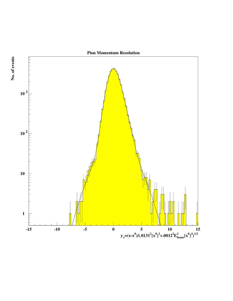
Figure 6.5: The number of events as a function of $y_{\mu}$ given in a logarithmic scale. The solid line is our parametrization which represent the energy resolution ${\cal R}$.

Fig. 6.5 and 6.6 show the resulting $y_{\pi}$ and $y_{\mu}$ distributions respectively. These distributions contain non-Gaussian tails. Therefore, they are parametrized as sums of three Gaussians with different width, mean and normalization parameters

$${\cal R}(x^{0},\mbox{$x$},\mbox{$\cos\theta$})=\sum_{i=1}^{3}\rho_{i}\exp\left[-\frac{1}{2}\left(\frac{y-\bar{y}_{i}}{\sigma_{i}}\right)^{2}\right].$$ (6.17)

The values of the fit parameters and their errors are listed in Tables 6.5 and 6.6 . The $\chi^{2}/D.O.F.$ values of the fit are 61/53 and 54/64 for the $\tau$$\rightarrow$$\pi$(K)$\nu_{\tau}$ and $\tau$$\rightarrow$$\mu$$\bar{\nu}_{\mu}$$\nu_{\tau}$ respectively.

.

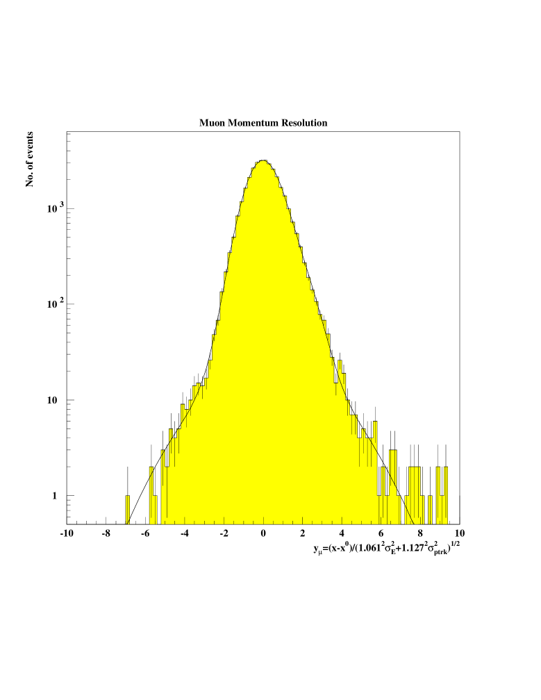
Figure 6.6: The number of events as a function of $y_{\mu}$ given in a logarithmic scale. The solid line is our parametrization which represent the energy resolution ${\cal R}$.

i	1	2	3
norm., $\rho_{i}$	1.	0.292$\pm$0.031	0.016 $\pm$ 0.012
mean, $\bar{y}_{i}$	-0.023$\pm$0.020	0.528$\pm$0.049	0.51$\pm$0.11
width, $\sigma_{i}$	0.818$\pm$0.010	1.22$\pm$0.072	2.57$\pm$0.44

Table 6.5: Parameters of the three Gaussians describing the exact shape of the pion $x$ resolution function.

i	1	2	3
norm., $\rho_{i}$	1.	0.2732$\pm$0.0048	0.0098$\pm$0.0037
mean, $\bar{y}_{i}$	-0.057$\pm$0.010	0.427$\pm$0.030	0.36$\pm$0.14
width, $\sigma_{i}$	0.7266$\pm$0.0071	1.127$\pm$0.029	2.60$\pm$0.

Table 6.6: Parameters of the three Gaussians describing the exact shape of the muon $x$ resolution function.

.

Figure 6.7: $x$ vs. $\cos\theta$ for data $\mu$-pairs.

We considered the following contributions to the systematic error associated with the muon and pion resolution function.

• The uncertainties in the parameters of the resolution functions coming from the limited statistics of the $\mu$-pair sample. We used the errors listed in Tables 6.5 and 6.6 including their correlations in order to propagate them to the final results.

• We investigated a possible dependence of the momentum measurement on $\cos\theta$. Such dependence could result from a possible twist of the two end-plates of the jet chamber, that will result in a tracks distortion so that the measured momentum would be larger or smaller than the true value, depending on the charge and $\cos\theta$ values. In this case, there would be a net bias in the A${}_{pol}^{FB}$ measurement. Fig. 6.7 shows a scatter plot of $x$ vs. $\cos\theta$ for $\mu$-pairs data which looks uniform. dividing the $\cos\theta$ range into 14 intervals, average over $x$ for each interval, and fitting $\bar{x}$ to $a(1+b\mbox{$\cos\theta$})$ we obtain $b=(-1.99\pm 0.94)\cdot 10^{-3}$ with $\chi^{2}/D.O.F.$=11.8/12. We introduced this small $b$ value in our ML fit the effect on the final results was found to be very small (see Table 6.7).

• We investigated whether there is any dependence of the $y_{\mu,\pi}$ distribution on $|\cos\theta|$, by considering separate distributions from MC $\tau$$\rightarrow$$\mu$$\bar{\nu}_{\mu}$$\nu_{\tau}$ decays for $|\cos\theta|$ below and above 0.35. The obtained RMS values were 0.0716 and 0.0759. Assuming a linear dependence of the RMS on $|\cos\theta|$, we multiplied $y_{\mu,\pi}$ by $0.996+0.011\mbox{$|\cos\theta|$}$ and the obtained deviations in $\langle P_{\tau}\rangle$ and A${}_{pol}^{FB}$ are listed in Table 6.7.

Table 6.7 summarizes all the systematic errors associated with the muon and pion momentum resolutions. This amounts a total of $0.38\%$ and $0.21\%$ for $\langle P_{\tau}\rangle$ and A${}_{pol}^{FB}$, respectively.

	whole sample		$\tau$$\rightarrow$$\mu$$\bar{\nu}_{\mu}$$\nu_{\tau}$		$\tau$$\rightarrow$$\pi$ $\nu_{\tau}$
source	$\Delta\langle P_{\tau}\rangle$	$\Delta$ A${}_{pol}^{FB}$	$\Delta\langle P_{\tau}\rangle$	$\Delta$ A${}_{pol}^{FB}$	$\Delta\langle P_{\tau}\rangle$	$\Delta$ A${}_{pol}^{FB}$
$\mu$-pair statistics	0.10	0.01	0.47	0.03	0.10	0.01
$\mbox{$x$}-\mbox{$\cos\theta$}$ dep.	0.21	0.21	1.03	1.17	0.32	0.72
resolution $|\cos\theta|$ dep.	0.30	0.02	0.98	0.11	0.11	0.00
Total	0.38	0.21	1.50	1.18	0.35	0.72

Table 6.7: Systematic errors (in %) associated with the muon and pion resolution function.

Before concluding this sub-section, one should mention two other sources of systematic errors associated with the track measurement, which are related to the A${}_{pol}^{FB}$ determination.

• Uncertainty in $\cos\theta$ measurement may affect the A${}_{pol}^{FB}$ determination, since events near $\mbox{$\cos\theta$}=0$ can migrate from positive to negative $\cos\theta$ value and vice versa. It also introduces an inaccuracy in the cut on $|\cos\theta|$ at 0.68. The $|\cos\theta|$ value is obtained in our analysis by averaging the corresponding values of the two $\tau$-jets, taking into account tracks and EB clusters. This is a measure of the $|\cos\theta|$ of the tau and not just the track. Therefore, part of the inaccuracy in $\cos\theta$ results from the invisible $\nu$’s in the event. We investigated the $\cos\theta$ resolution using MC events and obtained an uncertainty of 0.0225. We introduced in our ML fit a resolution function in $\cos\theta$ using an error in $\cos\theta$ twice as large, in order to account for possible data-MC differences. The resulting variation in A${}_{pol}^{FB}$ is smaller than 0.05%.

• Wrong charge assignment of the $\tau$-jets, resulting in a wrong sign of $\cos\theta$. The charge assignment is done by the following algorithm: The charge of each $\tau$-jet is defined as the sum of its track charges. If both $\tau$-jets have opposite charges, there is no ambiguity. If one jet charge is zero, only the second jet charge is used. If both jets have the same charge and this charge is not zero, then the correct charge is taken from the jet with a smaller number of tracks. In the remaining cases where the two jets have the same number of tracks, we consider only the most energetic track from each $\tau$-jet and take the charge of the track with the smaller momentum. As a result of this procedure, only 0.35% of the events have a wrong charge assignment, as obtained from the MC sample. This would reduce the value of A${}_{pol}^{FB}$ by a negligible amount of $0.007\times\mbox{\rm A${}_{pol}^{FB}$}$. If we assume that in the data the situation is twice as bad, we end up with a systematic error in A${}_{pol}^{FB}$ of 0.16%.

In total, the systematic error in A${}_{pol}^{FB}$ associated with these two sources is 0.17%. This uncertainty is common to all decay channels.

6.3.2 The Resolution Function for Electrons

The electron energy is taken from the EM calorimeter. We are using the corrected EB energy and we include a further correction depending on the total presampler multiplicity in the cone. In order to investigate the possibility of using the PB data, we used Bhabha events and tested the EB energy normalized by the beam energy ($x_{EB}$) as a function of the PB multiplicity (number of hits). A decrease in the EB energy for increasing PB multiplicity is found as expected due to electrons which started showering in the material in front of The result of our study is following correction to $x_{e}$,

$$x_{e}=x_{\scriptscriptstyle EB}+0.02\times Max(N_{\scriptscriptstyle PB}-10,0)/\mbox{$E_{beam}$},$$ (6.18)

where $N_{\scriptscriptstyle PB}$ is the PB multiplicity.

In order to investigate the energy resolution dependence on its energy, we are using real Bhabha electrons data, single electron events and $\tau$$\rightarrow$e$\bar{\nu}_{e}$$\nu_{\tau}$ decays. For $\tau$$\rightarrow$e$\bar{\nu}_{e}$$\nu_{\tau}$ electrons we are using our analysis sample and the other events were selected using the standard cuts of the TP103 package [53]. For Bhabha events we required also an acollinearity below $0.2^{\circ}$, to reduce radiative effects similarly to our procedure with $\mu$-pairs.

The Bhabha electrons events are assumed to have the beam energy. We do not know the real energy of the electrons from the other sources but we can utilize their $E/p$ and $\Delta p/p$ distributions at different energies in order to obtain the energy resolution,

$$\frac{\Delta x}{x}=\frac{\Delta E}{E}=\sqrt{[\Delta(\frac{E}{p})/(\frac{E}{p})]^{2}-(\frac{\Delta p}{p})^{2}}.$$ (6.19)

The width $\Delta(E/p)$ is obtained by a Gaussian fit to the distribution of $E/p$ at the different energy points. For the evaluation of $\Delta p/p$ we use $\Delta p/p=C\sqrt{x^{4}+(0.3x)^{2}+0.02x}/x$ where the factor $C=0.073\pm 0.006$ is obtained from Bhabha and $\mu$-pair events.

.

Figure 6.8: $\Delta E/E$ dependence on $x$. The last point is calculated with Bhabha events and in the first three points it is done with single electrons. For consistency we plot also the $E/p$ of the $\tau$$\rightarrow$e$\bar{\nu}_{e}$$\nu_{\tau}$ events from our data sample. The line represents our parametrization to this dependence.

Fig. 6.8 presents the $\Delta E/E$ dependence on $x$. The resolution in the last point is estimated from the Bhabha events, whereas the first three points, were calculated with the single electrons. As a consistency check we also plot the results of the electrons from $\tau$$\rightarrow$e$\bar{\nu}_{e}$$\nu_{\tau}$ decays, using their $E/p$ distribution. The error bars of all these results derived from the statistical uncertainties of the $E/p$ widths and the error factor $C$.

The $\frac{\Delta E}{E}$ values were fitted by the function $a+b/\sqrt{x}$,

$$\frac{\Delta x}{x}=\frac{\Delta E}{E}=(0.0192\pm 0.0008)+(0.0139\pm 0.0008)/\sqrt{x}.$$ (6.20)

This is shown in Fig. 6.8 having a $\chi^{2}/D.O.F.$ of 4.7 for 6 D.O.F.

As for the muons and pions, we define $y_{e}$ for electrons as,

$$y_{e}=\frac{\mbox{$x$}-x^{0}}{0.0192x^{0}+0.0139\sqrt{x^{0}}}.$$ (6.21)

As before also here the second step is the study of the exact resolution shape, including the tails of the distribution. For the $\tau$$\rightarrow$e$\bar{\nu}_{e}$$\nu_{\tau}$ it is investigated by using Bhabha events describing them by a sum of three Gaussians as in Eq. 6.17.

Fig. 6.9 presents the $y_{e}$ distribution and our parametrization. The values of the fit parameters and their errors are listed in Table 6.8. The $\chi^{2}/D.O.F.$ of the fit is 74/58.

.

Figure 6.9: The number of events as a function of $y_{e}$ given in a logarithmic scale. The solid line is our parametrization which represent the energy resolution ${\cal R}$.

i	1	2	3
normalization, $\rho_{i}$	1	0.192 $\pm$ 0.032	0.0067 $\pm$ 0.0018
mean, $\bar{y}_{i}$	0.120 $\pm$ 0.010	0.00 $\pm$ 0.039	-1.72 $\pm$ 0.52
width, $\sigma_{i}$	0.571 $\pm$ 0.016	1.317 $\pm$ 0.067	4.65 $\pm$ 0.67

Table 6.8: Parameters of the three Gaussians describing the electron energy resolution functions.

Two sources of uncertainties contribute to the systematic error associated with the electron energy resolution.

• The errors on the energy dependence of the resolution (see Eq. 6.20).

• The errors on the parameters describing the exact shape of the resolution function, shown in Table 6.8.

These errors were propagated properly to the final results, taking also their correlations into account.

A summary of the systematic errors associated with the electron energy resolution is presented in Table 6.9. The uncertainty in the calorimeter response introduces total errors of $0.48\%$ for $\langle P_{\tau}\rangle$ and $0.12\%$ for A${}_{pol}^{FB}$.

	whole sample		$\tau$$\rightarrow$e$\bar{\nu}_{e}$$\nu_{\tau}$
source	$\Delta\langle P_{\tau}\rangle$	$\Delta$ A${}_{pol}^{FB}$	$\Delta\langle P_{\tau}\rangle$	$\Delta$ A${}_{pol}^{FB}$
energy dependence	0.01	0.00	0.04	0.01
resolution function	0.32	0.10	1.46	0.45
energy scale	0.37	0.07	2.23	0.17
Total	0.48	0.12	2.67	0.48

Table 6.9: Systematic errors (in %) associated with electron resolution function.

6.4 Tau-Pair Selection Efficiency

The efficiency of $\tau$-pair selection, ${\cal E}^{\pm}_{i}(\mbox{$x_{i}$},\mbox{$\cos\theta$})$, is investigated using the $\tau$-pair MC events and comparing the kinematic variable distributions before and after the selection requirements. This is done separately for events with positive and negative $\tau^{-}$ helicities and for the various combinations of the decays of the two taus.

When both $\tau$’s decay via one of the modes considered here (e, $\mu$ or $\pi$(K)), the efficiency is parametrized as a function of the kinematic variables $x_{i}$, $x_{j}$ and $\cos\theta$. When the selection requirements involve two or even all three kinematic variables in a correlated manner then these are explicitly taken into account in the parametrization of the efficiency.

The efficiency used in our fit (Eqs. 6.2 and 6.5) is expressed as a function of the measured variables, $x_{i}$ and $x_{j}$, on which all the cuts are applied. However, we cannot obtain the efficiency as a function of the measured variables since for events which were not identified as $\tau$-pairs, very often those variables are not defined. Therefore, we have to use the corresponding generated variables $\mbox{$x_{i}$}^{0}$ and $\mbox{$x_{j}$}^{0}$. As long as the variation of efficiency with the variables is weak, it should not make any difference. However, for those $\tau$-pair selection cuts which depend on $x_{i}$ and $x_{j}$ variable one has to be more careful and include this fact in the efficiency function. The three cuts which depend on $x_{i}$ and $x_{j}$ are T4, T5 and T6 and these are treated in the following way:

• The efficiency ${\cal E}^{\pm}_{ij}(\mbox{$x_{i}$},\mbox{$x_{j}$},\mbox{$\cos\theta$})$ to select $\tau$-pair events where both taus decay into the same channel is set to be 0 if $\mbox{$x_{i}$}+\mbox{$x_{j}$}<0.4$ and $(\mbox{$x_{i}$}-\mbox{$x_{j}$})\sin\theta<0.04$. This corresponds to the cut against two photon events (T4). This cut rejects events with low visible energy namely, if both missing transverse momentum calculated from the tracks and the from the EM clusters are below 2  $GeV$. It therefore affect mainly $\tau$-pair events where both taus decay to the same channel.

• The efficiency ${\cal E}^{\pm}_{ij}(\mbox{$x_{i}$},\mbox{$x_{j}$},\mbox{$\cos\theta$})$ to select events where both taus decay into electron is required to vanish when $\mbox{$x_{i}$}+\mbox{$x_{j}$}>1.6$. This is due to the rejection of Bhabha events with cut T5 which influence $\tau$-pair events of this type.

• The rejection of mu-pair events by cut T6 affects mainly events where both taus decay into muons. For such events, we require that
  $\mbox{${\cal E}^{\pm}_{ij}(\mbox{$x_{i}$},\mbox{$x_{j}$},\mbox{$\cos\theta$})$}=0$ when ${\mbox{\mbox{$x_{i}$}}+\mbox{$x_{j}$}>1.2}$. A possible residual effect of this cut on events with one $\tau$$\rightarrow$$\mu$$\bar{\nu}_{\mu}$$\nu_{\tau}$ and one $\tau$$\rightarrow$$\pi$(K)$\nu_{\tau}$ decays was taken into account by allowing a step function change in ${\cal E}^{\pm}_{ij}(\mbox{$x_{i}$},\mbox{$x_{j}$},\mbox{$\cos\theta$})$ at $\mbox{$x_{i}$}+\mbox{$x_{j}$}=1.2$.

To determine the $\tau$-pair selection efficiency we investigate $\tau$-pair MC events which satisfy the three cuts mentioned above. We consider the distributions of the kinematic parameters before and after the $\tau$-pair selection. The ratio between the distributions after and before the selection gives the efficiency of the selection excluding the cuts T4, T5 and T6. This procedure is done separately for positive and negative $\tau^{-}$ helicity events. The $|\cos\theta|$ dependence of the efficiency turns out to be constant over the whole region from 0 to 0.68 and that for all decay channel combinations.

In the case where both taus decay into electron, muon or pion, we have to consider in addition to $|\cos\theta|$ the two kinematic variables, $x_{i}$ and $x_{j}$. Therefore, we consider two-dimensional efficiency distributions in a 6$\times$6 regions in $x_{i}$ and $x_{j}$ and fit them using expression of the following form

$${\cal E}_{ij}(\mbox{$x_{i}$},\mbox{$x_{j}$}) = a_{1}(1+a_{2}\mbox{$x_{i}$}+a_{4}\mbox{$x_{i}$}^{2})(1+a_{3}\mbox{$x_{j}$}+a_{5}\mbox{$x_{j}$}^{2})$$ (6.22)

$$+a_{6}\mbox{$x_{i}$}\mbox{$x_{j}$}+a_{7}\mbox{$x_{i}$}^{2}\mbox{$x_{j}$}+a_{8}\mbox{$x_{i}$}\mbox{$x_{j}$}^{2}+a_{9}\mbox{$x_{i}$}^{2}\mbox{$x_{j}$}^{2}.$$

For $\mbox{$x_{i}$}<.05$ or $\mbox{$x_{j}$}<.05$ the efficiency is reduced by a factor, while if both $x_{i}$ and $x_{j}$ are $<.05$ then the efficiency is set to 0. The parameter $a_{1}$ is expected to be close to 1 and all other parameters are expected to be close to 0. If after

doing the fit any of the parameters turns out to be consistent within error with its expected value it is set to that value as a constant in the fit, and the fit is repeated. In this way we are using just the number of parameters necessary to obtain a reasonable fit.

When only one $\tau$ decays to e, $\mu$ or $\pi$(K) and the other $\tau$ decay is not identified, the selection efficiency has two components. The first accounts for the case where the other $\tau$ does not decay via e, $\mu$ or $\pi$(K) while the second accounts for the case where it does decay via these channels but could not be identified. The first component is parametrized as a function of $x_{i}$ and $\cos\theta$, checking that these two kinematic variables are not correlated. The second component, which arises from identification inefficiencies, can have correlations which were taken into account.

.

Figure 6.10: Tau-pair selection efficiencies as functions of $x$ for events where only one tau decays into electron (Figs. a,b), muon (Figs. c,d) or pion (Figs. e,f). Figs. a,c,e (b,d,f) correspond to positive (negative) helicity events.

In the cases where only one $\tau$ decay is identified, the selection efficiency ${\cal E}_{i}(\mbox{$x_{i}$})$ is parametrized as a quadratic function of just one variable, $x_{i}$. For $\mbox{$x_{i}$}<.05$ the efficiency, ${\cal E}_{i}(\mbox{$x_{i}$})$, is further reduced by a factor. Also here, when any parameter is obtained from the fit as consistent with its expected value (1 for the normalization and 0 for the others) it is set to the expected value and the fit is redone.

In Fig. 6.10 we plot the $\tau$-pair selection efficiencies as function of $x$ for these cases where only one tau decays to $e$, $\mu$ or $\pi(K)$ together with our parametrization. In Table 6.10 we list the $\chi^{2}$ values obtained in our parametrization fits.

Decay channel combination	positive helicity	negative helicity
a) $\tau$$\rightarrow$e$\bar{\nu}_{e}$$\nu_{\tau}$, none	13.6/16	15.2/16
b) $\tau$$\rightarrow$$\mu$$\bar{\nu}_{\mu}$$\nu_{\tau}$, none	12.6/15	12.6/14
c) $\tau$$\rightarrow$$\pi$(K)$\nu_{\tau}$, none	11.4/14	9.0/14
d) $\tau$$\rightarrow$e$\bar{\nu}_{e}$$\nu_{\tau}$, $\tau$$\rightarrow$e$\bar{\nu}_{e}$$\nu_{\tau}$	15.9/29	24.9/32
e) $\tau$$\rightarrow$e$\bar{\nu}_{e}$$\nu_{\tau}$, $\tau$$\rightarrow$$\mu$$\bar{\nu}_{\mu}$$\nu_{\tau}$	35.9/24	41.6/24
f) $\tau$$\rightarrow$e$\bar{\nu}_{e}$$\nu_{\tau}$, $\tau$$\rightarrow$$\pi$(K)$\nu_{\tau}$	18.9/27	41.7/24
g) $\tau$$\rightarrow$$\mu$$\bar{\nu}_{\mu}$$\nu_{\tau}$, $\tau$$\rightarrow$$\mu$$\bar{\nu}_{\mu}$$\nu_{\tau}$	19.4/29	29.4/32
h) $\tau$$\rightarrow$$\mu$$\bar{\nu}_{\mu}$$\nu_{\tau}$, $\tau$$\rightarrow$$\pi$(K)$\nu_{\tau}$	32.4/25	44.9/24
i) $\tau$$\rightarrow$$\pi$(K)$\nu_{\tau}$, $\tau$$\rightarrow$$\pi$(K)$\nu_{\tau}$	12.1/33	20.0/28

Table 6.10: $\chi^{2}/D.O.F.$ coming from the parametrization fits for $\tau$-pair selection efficiency.

The error coming from the $\tau$-pair selection efficiency is composed of the MC statistics and the error related to the resolution and scale uncertainties in the ECAL and tracking detector.

Systematic uncertainties in the efficiency resulting from the MC statistics were investigated by propagating the statistical errors in the parameters obtained from the parametrization fits to the final results as explained in Sect. 6.1.

As for possible effects in the data not fully modeled by the MC, we were concerned with the momentum and energy resolutions being broader in the real data as compared with the MC. In order to investigate this effect on the final results we used our MC event sample and smeared the generated track momenta and electron/photon energies according to our resolution functions obtained from real data control samples (see Sect. 6.3). After replacing those smeared values with the corresponding MC simulated ones, we recalculated the $\tau$-pair selection efficiencies and parametrized them in the same way as before. The different tau selection efficiency parametrization, calculated with and without additional smear to the MC, has a negligible effect to the overall uncertainty in $\langle P_{\tau}\rangle$ and in A${}_{pol}^{FB}$ of the order of 0.03% and 0.05% respectively. Nevertheless, we have used in the analysis the MC sample with an additional smear.

Table 6.11 summarizes the systematic errors associated with the $\tau$-pair selection efficiency for each decay channel separately.

	$\tau$$\rightarrow$e$\bar{\nu}_{e}$$\nu_{\tau}$		$\tau$$\rightarrow$$\mu$$\bar{\nu}_{\mu}$$\nu_{\tau}$		$\tau$$\rightarrow$$\pi$(K)$\nu_{\tau}$
	$\Delta\langle P_{\tau}\rangle$	$\Delta$ A${}_{pol}^{FB}$	$\Delta\langle P_{\tau}\rangle$	$\Delta$ A${}_{pol}^{FB}$	$\Delta\langle P_{\tau}\rangle$	$\Delta$ A${}_{pol}^{FB}$
error	1.10	0.80	0.59	0.06	0.36	0.08

Table 6.11: Systematic errors (in %) associated with $\tau$-pair selection efficiency. This is essentially based on the MC statistics.

Thus, the contributions from the tau selection efficiency to the overall uncertainty on $\langle P_{\tau}\rangle$ and A${}_{pol}^{FB}$ are 0.39% and 0.19%, respectively.

6.5 Efficiencies of the $\tau$ Decay Identification

The efficiencies to identify the various $\tau$ decays are obtained in two steps. In the first step, the MC events are used in order to obtain the efficiency distributions for each decay channel, separately for events with positive or negative $\tau^{-}$ helicity. These distributions depend on the $x$ variables of the identified $\tau$ and on $\cos\theta$. However, some of the identification requirements, such as those designed to remove Bhabha and mu-pair events, also introduce a dependence on the $x$ variable of the $\tau$ on the opposite side. This dependence is taken into account as described below.

For $\tau$$\rightarrow$e$\bar{\nu}_{e}$$\nu_{\tau}$ decays we refer to the cut against residual Bhabha events (cut E7) which rejects electron candidates when the other side has a single track with $x>.75$, and its acoplanarity is below $0.1^{\circ}$. Therefore, in evaluation of the $\tau$$\rightarrow$e$\bar{\nu}_{e}$$\nu_{\tau}$ identification efficiency, the events where the other tau decay into $e,\mu$ or $\pi$(K) were divided to those with the $x$ of the opposite side below and above 0.75. We did not find any statistically significant difference between the efficiency distributions of those event subsamples. In the case where the other $\tau$ do not decay into these three channels our criteria are independent of its $x$ value.

For the $\tau$$\rightarrow$$\mu$$\bar{\nu}_{\mu}$$\nu_{\tau}$ decay, the against $\mu$-pair events (cut M5) introduces a dependence on the opposite $\tau$ properties. This cut rejects muon candidates if the opposite jet is consistent with being a muon and has $x>0.8$. Hence, for events where both taus are identified as muons we require both $x$-values to be below 0.8. This condition is applied already in the parametrization of ${\cal E}^{\pm}_{ij}(\mbox{$x_{i}$},\mbox{$x_{j}$},\mbox{$\cos\theta$})$ and therefore does not have to be repeated. However there might be still some residual effects of this cut on events where the opposite jet contains a charged pion, which resemble a muon. Therefore, we investigated the $\tau$$\rightarrow$$\mu$$\bar{\nu}_{\mu}$$\nu_{\tau}$ identification efficiency for the following cases.

• events where the other tau does not decay into $e,\mu$ or $\pi$(K);

• events where the other tau decays into a lepton ($e,\mu$);

• events where the other side is a $\tau$$\rightarrow$$\pi$(K)$\nu_{\tau}$ decay with $x<0.8$;

• events where the other side is a $\tau$$\rightarrow$$\pi$(K)$\nu_{\tau}$ decay with $x>0.8$;

It turned out that for each case the identification efficiency was different. Moreover, for the third case, there was even a difference between positive and negative $\tau^{-}$ helicity events. This is due to the fact that the pions in positive $\tau$$\rightarrow$$\mu$$\bar{\nu}_{\mu}$$\nu_{\tau}$ helicity events are more energetic and thus are more sensitive to the cut. We had, therefore, to parametrize each case separately.

The efficiency plots for $\tau$$\rightarrow$e$\bar{\nu}_{e}$$\nu_{\tau}$, $\tau$$\rightarrow$$\mu$$\bar{\nu}_{\mu}$$\nu_{\tau}$ and $\tau$$\rightarrow$$\pi$(K)$\nu_{\tau}$ are given in Figs. 6.11-6.13 along with their parametrization curves. To allow a possible correlation between the efficiency dependencies on $x$ and $\cos\theta$ we use in the analysis a two-dimensional distribution and fit it to an expression which depends on both. The list of $\chi^{2}/D.O.F.$ values of all the efficiency fits are given in Table 6.12.

Decay channel combination	$\chi^{2}/D.O.F.$
$\tau$$\rightarrow$e$\bar{\nu}_{e}$$\nu_{\tau}$	17.7/27
$\tau$$\rightarrow$$\pi$(K)$\nu_{\tau}$	26.5/28
$\tau$$\rightarrow$$\mu$$\bar{\nu}_{\mu}$$\nu_{\tau}$, none	41.0/292
$\tau$$\rightarrow$$\mu$$\bar{\nu}_{\mu}$$\nu_{\tau}$, $\tau$$\rightarrow$$\ell$$\bar{\nu}_{\ell}$$\nu_{\tau}$	14.5/24
$\tau$$\rightarrow$$\mu$$\bar{\nu}_{\mu}$$\nu_{\tau}$, $\tau$$\rightarrow$$\pi$(K)$\nu_{\tau}$, $x<0.8$, pos. helicity	19.9/30
$\tau$$\rightarrow$$\mu$$\bar{\nu}_{\mu}$$\nu_{\tau}$, $\tau$$\rightarrow$$\pi$(K)$\nu_{\tau}$, $x<0.8$, neg. helicity	28.6/28
$\tau$$\rightarrow$$\mu$$\bar{\nu}_{\mu}$$\nu_{\tau}$, $\tau$$\rightarrow$$\pi$(K)$\nu_{\tau}$, $x>0.8$	25.5/28

Table 6.12: $\chi^{2}/D.O.F.$ of the parametrization fits for the $\tau$ decay identification.

.

Figure 6.11: Efficiencies of $\tau$$\rightarrow$e$\bar{\nu}_{e}$$\nu_{\tau}$ (a,b) and $\tau$$\rightarrow$$\pi$(K)$\nu_{\tau}$ (c,d) identification as functions of $x$ and $|\cos\theta|$.

.

Figure 6.12: Efficiencies of $\tau$$\rightarrow$$\mu$$\bar{\nu}_{\mu}$$\nu_{\tau}$ identification as function of $x$ and $|\cos\theta|$. In (a,b) the decay mode of the second hemisphere is not identified, where in (c,d) the second $\tau$ decays into a lepton.

.

Figure 6.13: Efficiencies of $\tau$$\rightarrow$$\mu$$\bar{\nu}_{\mu}$$\nu_{\tau}$ identification as function of $x$ and $|\cos\theta|$ for different cases (see also text).

Control samples

A shortcoming of efficiency evaluation based on MC distributions alone comes mainly from possible effects not modelled correctly in the detector simulation. Therefore, events from control samples of the data are used to correct the MC derived $\tau$ decay identification efficiency. The selection procedures of these control samples are largely independent of the $\tau$ decay identification requirements. The efficiencies obtained from those real data events are compared with those from MC simulating the same process and the same selection criteria. In this way, any bias due to the selection of the control sample itself is minimized.

For $\tau$$\rightarrow$e$\bar{\nu}_{e}$$\nu_{\tau}$ decay, Bhabha and single electron events are used. Fig. 6.14a shows the ratio between the efficiencies of the data and MC control samples, where the low energy points are from the single electron events and the high energy point is from the Bhabha events. The straight line fitted to these points parametrizes the correction which must be multiplied with the $\tau$$\rightarrow$e$\bar{\nu}_{e}$$\nu_{\tau}$ MC derived efficiency.

.

Figure 6.14: Corrections to the MC derived efficiencies for the tau identification using data control samples: a) for $\tau$$\rightarrow$e$\bar{\nu}_{e}$$\nu_{\tau}$ decay, using single electron and Bhabha events; b) for $\tau$$\rightarrow$$\mu$$\bar{\nu}_{\mu}$$\nu_{\tau}$ decay, using e⁺e^-$\rightarrow$e⁺e^-$\mu^{+}$$\mu^{-}$ and $\mu$-pairs; c) for $\tau$$\rightarrow$$\pi$(K)$\nu_{\tau}$ decay, using $\tau$$\rightarrow$$\rho$$\nu_{\tau}$ events (see text). The solid lines are our parametrization. The dotted lines in b) are alternative parametrization used to estimate the systematic uncertainties.

For Bhabha events, namely for high energy electrons, the efficiency calculated from the data is lower by 4.1% than the efficiency calculated with the MC Bhabha events. For single electron events, which are low energy electrons, the data efficiency is lower by 5% than the MC derived efficiency, leading to an energy dependent correction of $(0.949\pm 0.005)+(0.009\pm 0.005)\mbox{$x$}$.

In order to investigate the muon detection efficiency we used $\mu$-pair events for high energy and $\gamma\gamma$$\rightarrow$$\mu^{+}$$\mu^{-}$  events for low energy muons. The resulting correction for effects not modelled in the MC, shown in Fig. 6.14b, is $(0.961\pm 0.010)+(0.026\pm 0.010)\mbox{$x$}$. The uncertainty of these corrections, for both electrons and muons, is increased beyond the quoted errors of the fit parameters in order to allow for possible non-linear interpolations between the extreme $x$ regimes of the control samples.

For single charged pions or kaons there are no clean non-tau control samples available over the momentum range of interest. Instead, decays of the tau into hadronic states containing neutral pions and a single charged hadron are used. For example, the $\pi$(K) identification requirements that remove muons (see P4) can be controlled using the $\tau$$\rightarrow$$\rho$$\nu_{\tau}$ sample since these requirements are not used in the  $\tau$$\rightarrow$$\rho$$\nu_{\tau}$ identification. The resulting correction for these requirements is approximately uniformed equal to 0.98, but can also be parametrized as a second order polynomial. This ratio between data and MC is shown in Fig. 6.14c. We use the flat correction function, but investigate the effect of using the other alternative for the systematic study. We investigated this correction also separately for positive and negative $\cos\theta$ values and did not find any statistically significant difference.

In order to study the requirements designed to remove background containing neutral pions (see P3) an alternative pion selection based on a low jet mass requirement is used. This sample has larger background (12%), but is clean enough to estimate the systematic dependence of the results on the requirements on the presampler signal and unassociated ECAL clusters. The conclusion of this study is that the MC modelling of the $x$ dependence of the efficiency is in excellent agreement with the data. This is verified using a subsample of the $\tau$$\rightarrow$$\rho$$\nu_{\tau}$ events in which the neutral pion is well separated from the track and with a sample of very high momenta $\tau$$\rightarrow$$\pi$(K)$\nu_{\tau}$ events which had little background from the other hadronic decays. The statistical error obtained from this control sample investigation is taken to be a systematic error. The $\tau$$\rightarrow$$\rho$$\nu_{\tau}$ events are also used to demonstrate that the requirement that removes electrons (see P2), introduces a negligible contribution to the overall systematic error.

To conclude, three different sources of systematic errors associated with the decay identification efficiencies were considered.

• The MC statistics, i.e. the statistical errors of the parameters obtained by the fits to the MC efficiency distribution.

• Control sample statistics, i.e. the statistical errors is the parameters describing the corrections to the MC efficiencies obtained from the control samples. For the $\tau$$\rightarrow$$\pi$(K)$\nu_{\tau}$ channel we made an alternative fit to a non-flat line, $a+bx$, and we used the deviation of the $b$ parameter from 0 and its statistical error.

• Uncertainty in the interpolation of the corrections obtained from the control samples. This uncertainty refers only to the $\tau$$\rightarrow$e$\bar{\nu}_{e}$$\nu_{\tau}$ and $\tau$$\rightarrow$$\mu$$\bar{\nu}_{\mu}$$\nu_{\tau}$ channels where the control samples cover only very low and very high lepton energies. In order to estimate the effect of this uncertainty, we applied two alternative interpolations, in addition to the straight line between the two regions. These interpolations are described by the dotted lines in Figs. 6.14a,b.

The effect of each uncertainty was propagated to the final $\langle P_{\tau}\rangle$ and A${}_{pol}^{FB}$ results using the same method as used in the previous sections, and the results are summarized in Table 6.13. For each decay channel we list separately the effect on the $\langle P_{\tau}\rangle$ and on the A${}_{pol}^{FB}$ results of the whole sample, and on the results of a subsample containing the individual decay modes.

		whole sample		corr. subsample
source	$\tau$ decay	$\Delta\langle P_{\tau}\rangle$	$\Delta$ A${}_{pol}^{FB}$	$\Delta\langle P_{\tau}\rangle$	$\Delta$ A${}_{pol}^{FB}$
MC statistics	$\tau$$\rightarrow$e$\bar{\nu}_{e}$$\nu_{\tau}$	0.52	0.14	2.36	0.64
	$\tau$$\rightarrow$$\mu$$\bar{\nu}_{\mu}$$\nu_{\tau}$	0.20	0.08	0.85	0.34
	$\tau$$\rightarrow$$\pi$(K)$\nu_{\tau}$	0.77	0.07	1.42	0.13
	all	0.95	0.18
Control sample	$\tau$$\rightarrow$e$\bar{\nu}_{e}$$\nu_{\tau}$	0.15	0.00	0.68	0.01
	$\tau$$\rightarrow$$\mu$$\bar{\nu}_{\mu}$$\nu_{\tau}$	0.24	0.01	1.02	0.04
	$\tau$$\rightarrow$$\pi$(K)$\nu_{\tau}$	1.33	0.06	2.47	0.10
	all	1.51	0.06
Interpolation	$\tau$$\rightarrow$e$\bar{\nu}_{e}$$\nu_{\tau}$	0.04	0.00	0.18	0.01
	$\tau$$\rightarrow$$\mu$$\bar{\nu}_{\mu}$$\nu_{\tau}$	0.11	0.00	0.61	0.04
	all	0.11	0.01
All sources	$\tau$$\rightarrow$e$\bar{\nu}_{e}$$\nu_{\tau}$	0.52	0.14	2.46	0.64
	$\tau$$\rightarrow$$\mu$$\bar{\nu}_{\mu}$$\nu_{\tau}$	0.38	0.08	1.46	0.34
	$\tau$$\rightarrow$$\pi$(K)$\nu_{\tau}$	1.54	0.08	2.85	0.16
	Total	1.79	0.19

Table 6.13: Systematic errors (in %) associated with tau decay identification efficiencies.

These various efficiency corrections contribute systematic errors on $\langle P_{\tau}\rangle$ and A${}_{pol}^{FB}$ of 1.79% and 0.19%, respectively.

6.6 Background

As seen from Eqs. 6.2 and 6.5, the correction for background contamination in channel $i$ is performed separately for background from other $\tau$ decay sources ($\beta^{\pm}_{i}$) and background from non-$\tau$ sources ($\beta^{non-\mbox{$\tau$}}_{i(j)}$). There are two reasons for this separation of background sources.

• The background from other $\tau$ decay channels depends on the $\tau$ helicity of the event and therefore it must be calculated for each helicity separately.

• The background from non-$\tau$ events depends on the whole event, whereas the background from other $\tau$ decays depends only on the $\tau$-jet considered.

For these reasons we had to handle those two background types differently (see Eqs. 6.2, 6.5). In Section  6.6.1 we describe only the first background and in the next Section we shall present the second one.

6.6.1 Background from Other Tau Decay Channels

The background from other tau decays was initially investigated using our $\tau$-pair MC sample and separating between the two $\tau^{-}$ helicity states and between five decay channels, $\tau$$\rightarrow$e$\bar{\nu}_{e}$$\nu_{\tau}$, $\tau$$\rightarrow$$\mu$$\bar{\nu}_{\mu}$$\nu_{\tau}$, $\tau$$\rightarrow$$\pi$ $\nu_{\tau}$, $\mbox{$\tau$}\mbox{$\rightarrow$}h\pi^{0}\nu$ and combining all other channels together. The separation between the sources was done in order to be able to correct for the MC branching fractions of the different decay channels and to investigate systematics (see below). We considered separately the dependence of the background on the kinematic variables, $\beta^{\pm}_{i}(\mbox{$x_{i}$},\mbox{$\cos\theta$})$, and its overall normalization, $\bar{\beta}^{\pm}_{i}=\int d\mbox{$x$}_{i}d\mbox{$\cos\theta$}\mbox{$\beta^{\pm}_{i}(\mbox{$x_{i}$},\mbox{$\cos\theta$})$}$.

To obtain the overall normalization, we calculate the background fraction to channel $i$ from source $j$ by,

$$\bar{\beta}^{\pm}_{ij}=\frac{n^{MC}_{ij}}{n^{MC}_{ii}}\frac{c_{j}}{c_{i}},$$ (6.23)

where $n^{MC}_{ij}$ is the number of MC events from source $j$, identified as coming from channel $i$. The correction factor $c_{i}$ is the ratio between the branching fractions to channel $i$ in data and MC. For the branching fractions in the data of the $\tau$$\rightarrow$e$\bar{\nu}_{e}$$\nu_{\tau}$, $\tau$$\rightarrow$$\mu$$\bar{\nu}_{\mu}$$\nu_{\tau}$ $\tau$$\rightarrow$$\pi$(K)$\nu_{\tau}$ and $\mbox{$\tau$}\mbox{$\rightarrow$}h\pi^{0}\nu$ channels we are using the published OPAL results [7], [63]. No correction was applied to the background from the fifth source (all other channels). Table 6.14 lists the MC and data branching fractions.

	$\tau$$\rightarrow$e$\bar{\nu}_{e}$$\nu_{\tau}$	$\tau$$\rightarrow$$\mu$$\bar{\nu}_{\mu}$$\nu_{\tau}$	$\tau$$\rightarrow$$\pi$(K)$\nu_{\tau}$	$\mbox{$\tau$}\mbox{$\rightarrow$}h\pi^{0}\nu$
$B^{MC}$	18.25	17.76	12.59	24.77
$B^{data}$	17.62$\pm$0.47	16.80$\pm$0.41	12.22$\pm$0.59	26.27$\pm$0.61
$c=B^{data}/B^{MC}$	0.965$\pm$0.026	0.946$\pm$0.023	0.971$\pm$0.047	1.061$\pm$0.025

Table 6.14: Tau branching fractions (in %) used in our analysis.

The overall background fraction for channel $i$ is obtained by summing up the contributions from the five sources, $\bar{\beta}^{\pm}_{i}=\sum_{j=1}^{5}\bar{\beta}^{\pm}_{ij}$. Table 6.15 lists the various contributions to the background fractions and their sums.

$\tau^{-}$-hel.	positive			negative
$\tau$ decay	$\tau$$\rightarrow$e$\bar{\nu}_{e}$$\nu_{\tau}$	$\tau$$\rightarrow$$\mu$$\bar{\nu}_{\mu}$$\nu_{\tau}$	$\tau$$\rightarrow$$\pi$ $\nu_{\tau}$	$\tau$$\rightarrow$e$\bar{\nu}_{e}$$\nu_{\tau}$	$\tau$$\rightarrow$$\mu$$\bar{\nu}_{\mu}$$\nu_{\tau}$	$\tau$$\rightarrow$$\pi$ $\nu_{\tau}$
$\tau$$\rightarrow$e$\bar{\nu}_{e}$$\nu_{\tau}$		0.00	0.92		0.01	0.92
$\tau$$\rightarrow$$\mu$$\bar{\nu}_{\mu}$$\nu_{\tau}$	0.03		0.26	0.02		0.27
$\tau$$\rightarrow$$\pi$(K)$\nu_{\tau}$	2.34	1.01		2.68	1.76
$\mbox{$\tau$}\mbox{$\rightarrow$}h\pi^{0}\nu$	1.52	0.03	5.55	1.83	0.03	3.68
other	0.19	0.02	1.57	0.17	0.01	1.96
overall	4.08	1.06	8.30	4.70	1.81	6.83

Table 6.15: Background fractions (in %) to the three decay channels $\tau$$\rightarrow$e$\bar{\nu}_{e}$$\nu_{\tau}$, $\tau$$\rightarrow$$\mu$$\bar{\nu}_{\mu}$$\nu_{\tau}$, $\tau$$\rightarrow$$\pi$(K)$\nu_{\tau}$ (columns) from the various sources (rows).

.

Figure 6.15: Background from other tau decays as functions of $x$ to the channel $\tau$$\rightarrow$e$\bar{\nu}_{e}$$\nu_{\tau}$ (Figs. a,b), $\tau$$\rightarrow$$\mu$$\bar{\nu}_{\mu}$$\nu_{\tau}$ (Figs. c,d) and $\tau$$\rightarrow$$\pi$(K)$\nu_{\tau}$ (Figs. e,f). Figs. a,c,e (b,d,f) correspond to positive (negative) helicity events. In Figs. a,b contamination contributions from $\tau$$\rightarrow$$\pi$(K)$\nu_{\tau}$, $\tau$$\rightarrow$$\rho$$\nu_{\tau}$ and other $\tau$ decay channels (including $\tau$$\rightarrow$$\mu$$\bar{\nu}_{\mu}$$\nu_{\tau}$) are presented by open, hatched and cross-hatched histograms correspondingly. In Figs. c,d contamination contributions from $\tau$$\rightarrow$$\pi$(K)$\nu_{\tau}$ and all other $\tau$-decay channels are shown by open and hatched histograms correspondingly. In Figs. e,f contamination contributions from $\tau$$\rightarrow$$\rho$$\nu_{\tau}$, $\tau$$\rightarrow$e$\bar{\nu}_{e}$$\nu_{\tau}$, $\tau$$\rightarrow$$\mu$$\bar{\nu}_{\mu}$$\nu_{\tau}$ and other $\tau$ decays are drawn with open, hatched, black and cross-hatched histograms correspondingly. The curves are our parametrization. The vertical scale is in arbitrary units.

.

Figure 6.16: Background from other tau decays as functions of $|\cos\theta|$. to the channel $\tau$$\rightarrow$e$\bar{\nu}_{e}$$\nu_{\tau}$ (Figs. a,b), $\tau$$\rightarrow$$\mu$$\bar{\nu}_{\mu}$$\nu_{\tau}$ (Figs. c,d) and $\tau$$\rightarrow$$\pi$(K)$\nu_{\tau}$ (Figs. e,f). Figs. a,c,e (b,d,f) correspond to positive (negative) helicity events. In Figs. a,b contamination contributions from $\tau$$\rightarrow$$\pi$(K)$\nu_{\tau}$, $\tau$$\rightarrow$$\rho$$\nu_{\tau}$ and other $\tau$ decay channels (including $\tau$$\rightarrow$$\mu$$\bar{\nu}_{\mu}$$\nu_{\tau}$) are presented by open, hatched and cross-hatched histograms correspondingly. In Figs. c,d contamination contributions from $\tau$$\rightarrow$$\pi$(K)$\nu_{\tau}$ and all other $\tau$-decay channels are shown by open and hatched histograms correspondingly. In Figs. e,f contamination contributions from $\tau$$\rightarrow$$\rho$$\nu_{\tau}$, $\tau$$\rightarrow$e$\bar{\nu}_{e}$$\nu_{\tau}$, $\tau$$\rightarrow$$\mu$$\bar{\nu}_{\mu}$$\nu_{\tau}$ and other $\tau$ decays are drawn with open, hatched, black and cross-hatched histograms correspondingly. The curves are our parametrization. The vertical scale is in arbitrary units.

The dependence on the kinematic variables of the background fractions was also taken from the MC events. The $x$ and $\cos\theta$ MC background distributions for each helicity and decay channel, and from each source were fitted to third order polynomials. The normalization of each background source was then corrected by multiplying with the corresponding branching fraction correction $c$. The contributions from all sources were then summed up and normalized to $\bar{\beta}^{\pm}_{i}$. The resulting functions, $\beta^{\pm}_{i}(\mbox{$x_{i}$},\mbox{$\cos\theta$})$, are plotted in Figs. 6.15 and 6.16, together with the corrected MC distributions. The $\chi^{2}$ values for the agreement between the MC distributions and their polynomial parametrization are indicated on the plots.

For $\tau$$\rightarrow$e$\bar{\nu}_{e}$$\nu_{\tau}$, the background level from other $\tau$ decays is $\approx 4.7\%$, differing slightly between positive and negative $\tau^{-}$ helicity events, and originating mainly from $\tau$$\rightarrow$$\pi$(K)$\nu_{\tau}$ and $\tau$$\rightarrow$$\rho$$\nu_{\tau}$ decays. For $\tau$$\rightarrow$$\mu$$\bar{\nu}_{\mu}$$\nu_{\tau}$ this background is $\approx 1.5\%$ coming from $\tau$$\rightarrow$$\pi$(K)$\nu_{\tau}$ decays, and the background to $\tau$$\rightarrow$$\pi$(K)$\nu_{\tau}$ is $\approx 7.8\%$, mainly from $\tau$$\rightarrow$$\rho$$\nu_{\tau}$, $\mbox{$\tau$}\mbox{$\rightarrow$}\pi K^{0}\nu$ and $\tau$$\rightarrow$e$\bar{\nu}_{e}$$\nu_{\tau}$ decays. The MC expectations for these background levels are checked against the data by studying the tau jets that are identified in more than one decay channel and from studies of contaminations with Bhabha and muon-pair control samples.

The following contributions to the systematic error associated with the background from tau sources were considered.

• The uncertainties in the parameters of the background functions, originating from the statistics of our MC sample. An error on the $\mbox{$\tau$}\mbox{$\rightarrow$}\pi K^{0}\nu$ background is estimated by varying the MC expectation by $\pm 100\%$.

• A small ($<$0.1%) additional contribution to the errors arising from the experimental uncertainties in the tau branching ratios has been included to correct the MC numbers.

• Possible disagreement between the data and MC simulation. This was investigated in two ways.

  1. We used our Bhabha and $\mu$-pair control samples and counted the number of particles identified as pions. We compared these numbers for data and MC, and the ratios were 0.72$\pm$0.48 for electrons and 1.17$\pm$0.39 for pions. These ratios represent correction factors to be multiplied with the MC estimates of the background to $\tau$$\rightarrow$$\pi$(K)$\nu_{\tau}$ from $\tau$$\rightarrow$e$\bar{\nu}_{e}$$\nu_{\tau}$ and $\tau$$\rightarrow$$\mu$$\bar{\nu}_{\mu}$$\nu_{\tau}$ decays.

  2. We counted tau decays which were identified by two decay algorithms and compare it to MC. Almost all those identified as a pion and electron or as a pion and muon are pions (from MC). Therefore we can get a correction of the pions background to the electrons and muons. These corrections turn out to be 0.41$\pm$0.09 and 0.58$\pm$0.08 respectively. 50% of those identified as a rho and pion or electron or muon are $\rho$’s. Therefore we can get a correction to the background from rho to electron, muon and pion which are 1.30$\pm$0.10, 5.0$\pm$1.0 and 1.09$\pm$0.09.

  These corrections are applied in the systematic studies. We use either their uncertainties or their difference from the factor one (whichever greater) and see the corresponding effects on the final results.

Table 6.16 summarizes the systematic errors associated with the background from other tau decays. The contribution of the branching fraction uncertainties actually affect not only the background estimates but are used also in the expression for ${\cal E}^{\mbox{\small$\prime$}\pm}_{i}(\mbox{$x_{i}$},\mbox{$\cos\theta$})$ (Eq. 6.1) and in the estimate of the $\pi/K$ mass threshold effect.

	all		$\tau$$\rightarrow$e$\bar{\nu}_{e}$$\nu_{\tau}$		$\tau$$\rightarrow$$\mu$$\bar{\nu}_{\mu}$$\nu_{\tau}$		$\tau$$\rightarrow$$\pi$(K)$\nu_{\tau}$
source	$\Delta\langle P_{\tau}\rangle$	$\Delta$ A${}_{pol}^{FB}$	$\Delta\langle P_{\tau}\rangle$	$\Delta$ A${}_{pol}^{FB}$	$\Delta\langle P_{\tau}\rangle$	$\Delta$ A${}_{pol}^{FB}$	$\Delta\langle P_{\tau}\rangle$	$\Delta$ A${}_{pol}^{FB}$
MC	0.29	0.04	0.50	0.09	0.44	0.06	0.45	0.05
Data	0.58	0.09	1.49	0.06	0.25	0.16	0.10	0.01
Diff	0.32	0.02	0.15	0.08	0.22	0.01	0.49	0.02
Total	0.72	0.10	1.58	0.13	0.55	0.17	0.67	0.05

Table 6.16: Systematic errors (in %) associated with background from other tau decays and tau branching fractions. MC, Data, and BR stand for MC statistics, the difference between data and MC and Branching ratio fraction respectively.

These background sources contribute errors of 0.72% and 0.10% on  $\langle P_{\tau}\rangle$ and  A${}_{pol}^{FB}$, respectively.

6.6.2 Background from non-tau Events

Concerning the residual non-$\tau$ background after the selection criteria, the following sources are considered.

• e⁺e^-$\rightarrow$$\mu^{+}$$\mu^{-}$. This source mainly contaminates events where one $\tau$ is identified as $\tau$$\rightarrow$$\mu$$\bar{\nu}_{\mu}$$\nu_{\tau}$ decay and the other as $\tau$$\rightarrow$$\pi$(K)$\nu_{\tau}$ or when one tau is identified as a $\tau$$\rightarrow$$\mu$$\bar{\nu}_{\mu}$$\nu_{\tau}$ and the other is not identified, at the level of $0.4\%$ and $1.3\%$, respectively.

• e⁺e^-$\rightarrow$e⁺e^-$\mu^{+}$$\mu^{-}$. This source contributes only to events with two identified muons or one identified muon and an unidentified tau, at the level of $1.6\%$ and $0.3\%$ respectively.

• e⁺e^-$\rightarrow$e⁺e^-. This source contributes background to events where only one $\tau$ decay is identified as e or $\pi$(K) and the other tau decay is unidentified, and events where both decays are identified as $\tau$$\rightarrow$e$\bar{\nu}_{e}$$\nu_{\tau}$. The corresponding contamination levels are $0.3\%$, $0.2\%$ and $0.3\%$, respectively.

• e⁺e^-$\rightarrow$e⁺e^-e⁺e^-. This source contaminates only events with one electron where the opposite tau decay is unidentified or two identified electrons, at the level of $0.3\%$ and $2.6\%$, respectively.

• $\mbox{\mbox{\rm e${}^{+}$}\mbox{\rm e${}^{-}$}}\mbox{$\rightarrow$}q\bar{q}$. The background from this source is negligible for all channels considered here.

The $\beta^{non-\mbox{$\tau$}}_{i(j)}(\mbox{$x_{i}$},\mbox{$x_{j}$},\mbox{$\cos\theta$})$ correction functions for each source were initially determined using the corresponding MC event samples. In practice the correlations between $x$_i(j)  and $\cos\theta$ are small and the $\beta^{non-\mbox{$\tau$}}_{i(j)}$ functions factorize into products of simple functions. These were adjusted by factors obtained from comparisons between the data and MC when the tau selection requirements designed to suppress these backgrounds were loosened.

Table 6.17 lists the five sources which were considered where for each source the size of the MC sample is quoted. These numbers were estimated from the integrated luminosity collected by OPAL during 1990-1992. In addition, we list the expected background fraction for each combination of decay channels.

source	$ee\mbox{$\rightarrow$}\mu\mu$	$ee\mbox{$\rightarrow$}q\bar{q}$	$ee\mbox{$\rightarrow$}ee$	$ee\mbox{$\rightarrow$}ee\mu\mu$	$ee\mbox{$\rightarrow$}eeee$	total
MC	200000	702400	46187∗	50.23 pb-1	42.98 pb-1
$e$, none	0.05$\pm$0.02	0.00	0.31$\pm$0.12	0.00	0.25$\pm$0.08	0.61$\pm$0.15
$\mu$, none	1.29$\pm$0.09	0.00	0.00	0.26$\pm$0.08	0.00	1.55$\pm$0.12
$\pi$, none	0.00	0.00	0.18$\pm$0.13	0.00	0.00	0.18$\pm$0.13
$e$, $e$	0.00	0.00	0.28$\pm$0.28	0.00	2.60$\pm$0.65	2.88$\pm$0.71
$e$, $\mu$	0.14$\pm$0.05	0.00	0.00	0.00	0.00	0.14$\pm$0.05
$\mu$, $\mu$	0.05$\pm$0.02	0.00	0.00	1.60$\pm$0.40	0.00	1.65$\pm$0.40
$\mu$, $\pi$	0.40$\pm$0.16	0.00	0.00	0.00	0.00	0.40$\pm$0.16
∗ numbers correspond to $\mbox{$|\cos\theta|$}<0.9$

Table 6.17: Non-tau background sources and their relative contributions (in %) to the various combinations of $\tau$ decay channels. The combinations not mentioned in this table have no background.

The $x$ and $\cos\theta$ dependence was taken from the MC distributions and parametrized by simple functions. Fig. 6.17 shows these distributions for those decay channel combinations where the overall non-tau background is above 0.5%.

.

Figure 6.17: Background from non-tau sources to events with one identified $\tau$$\rightarrow$e$\bar{\nu}_{e}$$\nu_{\tau}$ and the other side not identified (a,b); events with two identified $\tau$$\rightarrow$e$\bar{\nu}_{e}$$\nu_{\tau}$ (c,d); events with one identified $\tau$$\rightarrow$$\mu$$\bar{\nu}_{\mu}$$\nu_{\tau}$ and the other side not identified (e,f); events with two identified $\tau$$\rightarrow$$\mu$$\bar{\nu}_{\mu}$$\nu_{\tau}$ (g,h). Figs. a,c,e,g (b,d,f,h) show the $x$ ($\cos\theta$) dependence. In Figs. a-d, the open, hatched and cross-hatched histograms represent the background from Bhabha, $ee\mbox{$\rightarrow$}eeee$ and $\mu$-pairs respectively. In Figs. e-h, the open and hatched histograms are the background from $\mu$-pairs and $ee\mbox{$\rightarrow$}ee\mu\mu$ respectively. The dashed lines are our parametrization. The vertical scale is in arbitrary units.

Two sources of systematic errors associated with the non-tau background were considered.

• Finite statistics of our MC event samples, illustrated by the given errors in Table 6.17. To estimate their effect, we varied both the background levels and the parametrization of their $x$ ans $\cos\theta$ dependence within the statistical errors and examined the effect on the final results.

• Possible incompatibility between MC and data. This was investigated by J. Clayton [62] using background enriched subsample where he obtained correction factors for all the non-tau background sources. As we did for the tau background, we apply these correction factors only for the systematic study. We use either their uncertainties or their difference from the value one (whichever greater) and observe the corresponding effects on the final results.

Table 6.18 summarized the systematic errors associated with the non-tau background.

	all		$\tau$$\rightarrow$e$\bar{\nu}_{e}$$\nu_{\tau}$		$\tau$$\rightarrow$$\mu$$\bar{\nu}_{\mu}$$\nu_{\tau}$		$\tau$$\rightarrow$$\pi$(K)$\nu_{\tau}$
source	$\Delta\langle P_{\tau}\rangle$	$\Delta$ A${}_{pol}^{FB}$	$\Delta\langle P_{\tau}\rangle$	$\Delta$ A${}_{pol}^{FB}$	$\Delta\langle P_{\tau}\rangle$	$\Delta$ A${}_{pol}^{FB}$	$\Delta\langle P_{\tau}\rangle$	$\Delta$ A${}_{pol}^{FB}$
MC	0.48	0.16	1.56	0.60	1.20	0.17	0.33	0.15
Diff	0.48	0.08	0.72	0.26	1.97	0.26	0.07	0.03
Total	0.68	0.18	1.72	0.65	2.31	0.31	0.34	0.15

Table 6.18: Systematic errors (in %) associated with the non-tau background. MC and Data stand for the MC statistics and the difference between data and MC.

The contribution to the errors on $\langle P_{\tau}\rangle$ and A${}_{pol}^{FB}$ from the non-tau background corrections are 0.68% and 0.18%, respectively.

Chapter 7 Results and Cross Checks

7.1 Maximum Likelihood Fit Results

The ML fit, applied to the $\tau$$\rightarrow$e$\bar{\nu}_{e}$$\nu_{\tau}$, $\tau$$\rightarrow$$\mu$$\bar{\nu}_{\mu}$$\nu_{\tau}$ and $\tau$$\rightarrow$$\pi$(K)$\nu_{\tau}$ decay channels yields the following results,

$$\langle P_{\tau}\rangle = (-13.5\pm 2.9(stat))\%$$

A$${}_{pol}^{FB} = (-11.0\pm 3.5(stat))\%$$ (7.1)

where the correlation between the two numbers is 0.03.

The $\tau$  W $\nu_{\mbox{$\tau$}}$ Coupling

Since the $\tau$ decays via weak interaction, where parity is not conserved, the angular distribution of its decay products in the $\tau$ rest frame depends strongly both on the $\tau$ spin orientation and the characteristics of its charged weak decay process. The results given in the previous paragraph were calculated using the theoretical Eq. 4.37 which assume a $V-A$ structure for the $\tau$ decay. However, following Sect. 4.3 one can use the more general expression presented in Eq. 4.48, and extract not only the $\tau$ production parameters but also its decay parameters. Our results of a six parameters ML fit to the two polarization asymmetries and the Michel parameters $\rho,\delta,\xi$ and $\xi_{had}$ are:

$$\langle P_{\tau}\rangle = (-11.8\pm 3.2(stat))\%$$

A$${}_{pol}^{FB} = (-11.8\pm 3.7(stat))\%$$

$$\xi = 0.83\pm 0.18(stat)$$ (7.2)

$$\xi_{had} = 1.13\pm 0.16(stat)$$

$$\rho = 0.77\pm 0.01(stat)$$

$$\delta = 0.87\pm 0.13(stat)$$

which are consistent with a $(V-A)(V-A)$ structure (see Table 4.2).

The existing measurements of the Michel parameters are already precise enough to exclude interaction different from $V-A$ in the $\ell\mbox{$\bar{\nu}_{\ell}$}$ vertex ($\ell$=e,$\mu$), therefore one can use Eqs. 4.3 to evaluate the helicity of the $\nu_{\tau}$ from its relations with all last four parameters. This was further checked by fixing the $l\bar{\nu_{l}}$ vertex structure and allow only one free parameter to determine the characteristic of the $\mbox{$\tau$}\bar{\nu_{\mbox{$\tau$}}}$ vertex. The fit results are:

$$\langle P_{\tau}\rangle = (-12.3\pm 2.8(stat))\%$$

A$${}_{pol}^{FB} = (-11.4\pm 3.4(stat))\%$$

$$h_{\nu_{\mbox{$\tau$}}} = -1.06\pm 0.02(stat)$$ (7.4)

The measurement of the chirality parameter and the leptonic Michel parameters are all consistent with a $h_{\nu_{\mbox{$\tau$}}}=-1$ which is expected from a pure $V-A$ coupling at the $\mbox{$\tau$}\bar{\nu_{\mbox{$\tau$}}}$ vertex. It is also an indication for the $\nu_{\mbox{$\tau$}}$ being a left handed particle.

7.2 Summary of Systematic Studies

Table 7.1 summarizes the systematic errors in the ML analysis. Each error listed in Table 7.1 is a combined result of several related contributions. Since are no correlations between entries on different rows of the table, they are combined in quadrature to give the overall error listed in the last row. Thus, the values of the systematic errors of $\langle P_{\tau}\rangle$ and A${}_{pol}^{FB}$ using the $\tau$$\rightarrow$e$\bar{\nu}_{e}$$\nu_{\tau}$, $\tau$$\rightarrow$$\mu$$\bar{\nu}_{\mu}$$\nu_{\tau}$ and $\tau$$\rightarrow$$\pi$(K)$\nu_{\tau}$ decays are measured to be

$$\Delta\mbox{$\langle P_{\tau}\rangle$} = \pm 2.2\%(sys.)$$

$$\Delta\mbox{\rm A${}_{pol}^{FB}$} = \pm 0.5\%(sys.).$$ (7.6)

Source	$\Delta\langle P_{\tau}\rangle$	$\Delta$ A${}_{pol}^{FB}$
	(%)	(%)
$\tau$ decay identification	1.79	0.19
backg. from other $\tau$ decays	0.72	0.10
radiative effects	0.29	0.03
backg. from non-$\tau$ events	0.68	0.18
$\tau$-pair selection efficiency	0.39	0.20
calorimeter response	0.48	0.12
tracking response	0.38	0.21
AFB and K mass threshold	0.10	0.07
$\cos\theta$ and charge measurement	0.00	0.17
Total	2.19	0.43

Table 7.1: Summary of systematic uncertainties in the determination of $\langle P_{\tau}\rangle$ and A${}_{pol}^{FB}$ using $\tau$$\rightarrow$e$\bar{\nu}_{e}$$\nu_{\tau}$, $\tau$$\rightarrow$$\mu$$\bar{\nu}_{\mu}$$\nu_{\tau}$ and $\tau$$\rightarrow$$\pi$(K)$\nu_{\tau}$ channels .

The largest contribution to the systematic error of $\langle P_{\tau}\rangle$ is derived from the uncertainties in the efficiency of the $\tau$ decay mode identification. For the most part these arise from the limited statistics of the control samples, and in particular, the $\tau$$\rightarrow$$\rho$$\nu_{\tau}$ sample used to correct the efficiency of $\tau$$\rightarrow$$\pi$(K)$\nu_{\tau}$ identification. Therefore, one can expect that the systematic errors will decrease as more data is collected.

7.3 Monte Carlo checks

7.3.1 MC test of polarization biases

In order to check for potential biases in the fitting method, the analysis was performed on the $\tau$-pair MC sample. The ML fit is performed on the MC events, removing the corrections to the $\tau$ identification efficiencies derived from the data, and using resolution parameters extracted exclusively from MC events. Non-tau background correction is also switched off, since our sample contains only $\tau$-pair events. The input values for $\langle P_{\tau}\rangle$ and A${}_{pol}^{FB}$ are $-14.0$% and $-10.5$%, respectively and the fit returns values of ($-13.9\pm$1.0)% and ($-8.9\pm$1.3)%.

The fit results are listed in Table 7.2 which is similar to Table 7.3 for the data.

	$\langle P_{\tau}\rangle$	A${}_{pol}^{FB}$	Number of Events
Decay Channels	(%)	(%)
All decays	-13.9 $\pm$ 1.0	-8.9 $\pm$ 1.3	93462
1 $\tau$ identified	-13.9 $\pm$ 1.3	-8.5 $\pm$ 1.6	67199
(a) $\tau$$\rightarrow$e$\bar{\nu}_{e}$$\nu_{\tau}$, none	-11.9 $\pm$ 3.2	-5.5 $\pm$ 3.6	27058
(b) $\tau$$\rightarrow$$\mu$$\bar{\nu}_{\mu}$$\nu_{\tau}$, none	-15.6 $\pm$ 3.2	-8.1 $\pm$ 3.6	27120
(c) $\tau$$\rightarrow$$\pi$(K)$\nu_{\tau}$, none	-13.9 $\pm$ 1.7	-9.6 $\pm$ 2.0	13021
2 $\tau$’s identified	-13.9 $\pm$ 1.7	-9.5 $\pm$ 2.1	26263
(d) $\tau$$\rightarrow$e$\bar{\nu}_{e}$$\nu_{\tau}$, $\tau$$\rightarrow$e$\bar{\nu}_{e}$$\nu_{\tau}$	-8.9 $\pm$ 5.7	-15.0 $\pm$ 6.6	4684
(e) $\tau$$\rightarrow$e$\bar{\nu}_{e}$$\nu_{\tau}$, $\tau$$\rightarrow$$\mu$$\bar{\nu}_{\mu}$$\nu_{\tau}$	-13.7 $\pm$ 3.6	-8.3 $\pm$ 4.2	10328
(f) $\tau$$\rightarrow$e$\bar{\nu}_{e}$$\nu_{\tau}$, $\tau$$\rightarrow$$\pi$(K)$\nu_{\tau}$	-16.7 $\pm$ 3.2	-8.2 $\pm$ 4.0	3183
(g) $\tau$$\rightarrow$$\mu$$\bar{\nu}_{\mu}$$\nu_{\tau}$, $\tau$$\rightarrow$$\mu$$\bar{\nu}_{\mu}$$\nu_{\tau}$	-19.3 $\pm$ 9.4	0. $\pm$ 11.	4289
(h) $\tau$$\rightarrow$$\mu$$\bar{\nu}_{\mu}$$\nu_{\tau}$, $\tau$$\rightarrow$$\pi$(K)$\nu_{\tau}$	-13.4 $\pm$ 3.3	-9.1 $\pm$ 4.0	3195
(i) $\tau$$\rightarrow$$\pi$(K)$\nu_{\tau}$, $\tau$$\rightarrow$$\pi$(K)$\nu_{\tau}$	-9.4 $\pm$ 6.3	-19.5 $\pm$ 8.2	584
Average	-13.9 $\pm$ 1.0	-8.9 $\pm$ 1.3
$\chi^{2}/D.O.F.$	3.2/8	4.4/8
$\chi^{2}$ probability (%)	92.4	81.8

Table 7.2: $\tau$ polarization results (in %) from our MC sample. The average values the $\chi^{2}/D.O.F.$ and the $\chi^{2}$ probabilities correspond to the combined results of the 9 different channels (a) to (i). The input values are $\mbox{$\langle P_{\tau}\rangle$}=-14.0$% and $\mbox{\rm A${}_{pol}^{FB}$}=-10.5$%.

Although these values are consistent with the input values, we have changed the input parameters from purely negative to purely positive $\tau^{-}$ helicity and studied the dependence of the measured asymmetries on the input ones. Fig. 7.1 illustrates this investigation for the three individual channels as well as for the whole sample. We find no evidence for a bias in our measurement method.

.

Figure 7.1: Test of Bias in the $\langle P_{\tau}\rangle$ measurement. The error in the measurement of $\langle P_{\tau}\rangle$ as a function of the MC input polarization. Fig. a) - c) are for the $\tau$$\rightarrow$e$\bar{\nu}_{e}$$\nu_{\tau}$, $\tau$$\rightarrow$$\mu$$\bar{\nu}_{\mu}$$\nu_{\tau}$ and $\tau$$\rightarrow$$\pi$(K)$\nu_{\tau}$ respectively and d) present the results of all three channels together.

7.3.2 Check of the various parametrization using MC

For an overall check of our parametrization of the various corrections obtained from MC, we plot the MC $x$ distributions separately for each decay combination and compare it with the corresponding corrected theoretical curves (Figs. 7.2, 7.3, 7.4, 7.5). The $\chi^{2}$ values indicated on the figures show that the agreement between the MC distributions and the theoretical curves is good.

.

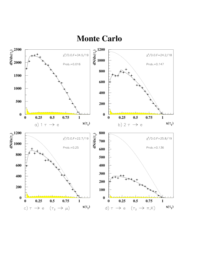
Figure 7.2: MC $x$ distributions for the $\tau$$\rightarrow$e$\bar{\nu}_{e}$$\nu_{\tau}$ decay channels and for various decays on the opposite side, compared with the theoretical predictions (solid lines) with all corrections included, taking the $\langle P_{\tau}\rangle$ value obtained from the global ML fit. The filled area represent the background part of the spectrum. The dotted lines are the uncorrected theoretical curves.

.

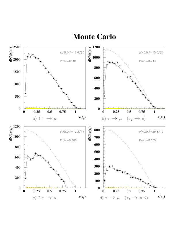
Figure 7.3: MC $x$ distributions of the $\tau$$\rightarrow$$\mu$$\bar{\nu}_{\mu}$$\nu_{\tau}$ decay channels and for various decays on the opposite side, compared with the theoretical predictions (solid lines) with all corrections included, taking the $\langle P_{\tau}\rangle$ value obtained from the global ML fit. The filled area represent the background part of the spectrum. The dotted lines are the uncorrected theoretical curves.

.

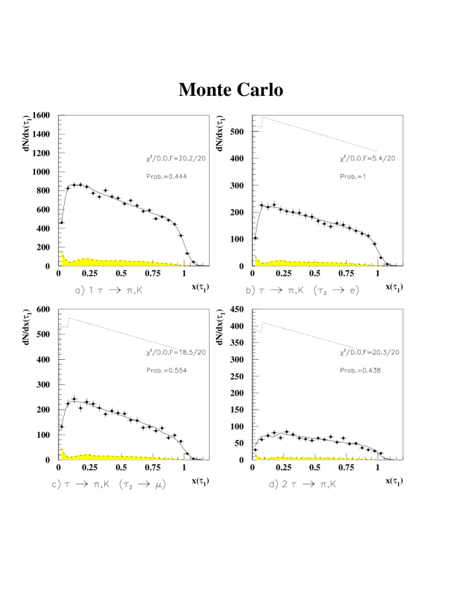
Figure 7.4: MC $x$ distributions for the $\tau$$\rightarrow$$\pi$(K)$\nu_{\tau}$ decay channels and for various decays on the opposite side, compared with the theoretical predictions (solid lines) with all corrections included, taking the $\langle P_{\tau}\rangle$ value obtained from the global ML fit. The filled area represent the background part of the spectrum. The dotted lines are the uncorrected theoretical curves.

.

Figure 7.5: MC $x$ distributions for the $\tau$$\rightarrow$e$\bar{\nu}_{e}$$\nu_{\tau}$, $\tau$$\rightarrow$$\mu$$\bar{\nu}_{\mu}$$\nu_{\tau}$ and $\tau$$\rightarrow$$\pi$(K)$\nu_{\tau}$ decays channels, summing over all decays on the other side and compared with the theoretical predictions (solid lines) with all corrections included, taking the $\langle P_{\tau}\rangle$ value obtained from the global ML fit. The filled area represent the background part of the spectrum. The dotted lines are the uncorrected theoretical curves.

7.4 Cross Checks

7.4.1 Statistical error examination

In order to convince ourselves that the statistical errors obtained from the fit are correct, we used a large sample of generated events without detector simulation and perform a simple ML fit to each decay, ignoring the other side and ommiting the corrections. We only applied the $x>0.05$ and $\mbox{$|\cos\theta|$}<0.68$ requirements. The errors obtained, after scaling them for the different numbers of events, were consistent with the statistical error obtained in our global fit within 3%.

7.4.2 Separate checks with the different decay topologies

The data has also been classified into nine independent subsamples, corresponding to all possible combinations of both $\tau$ decays excluding an identified $\tau$$\rightarrow$$\rho$$\nu_{\tau}$ decay. Doing this, nine independent results for $\langle P_{\tau}\rangle$ and A${}_{pol}^{FB}$ are obtained. These are listed in Table 7.3. The weighted mean of these values are within 0.3% of the global fit results and the $\chi^{2}$ probabilities for the consistency between the nine results for $\langle P_{\tau}\rangle$ and A${}_{pol}^{FB}$ are 17.2% and 81.6%, respectively.

Decay Channel combination	$\langle P_{\tau}\rangle$	A${}_{pol}^{FB}$	Number of Events
	(%)	(%)
Global fit value	$-13.5\pm$ 2.9	$-11.0\pm$ 3.5	12397
1 $\tau$ identified	$-17.5\pm$ 3.5	$-10.2\pm$ 4.3	9250
(a) $\tau$$\rightarrow$e$\bar{\nu}_{e}$$\nu_{\tau}$, none	$-24.7\pm$ 8.9	$-17.\pm$10.	3585
(b) $\tau$$\rightarrow$$\mu$$\bar{\nu}_{\mu}$$\nu_{\tau}$, none	$-8.7\pm$ 7.9	$-10.8\pm$ 9.0	3897
(c) $\tau$$\rightarrow$$\pi$(K)$\nu_{\tau}$, none	$-18.4\pm$ 4.4	$-8.1\pm$ 5.5	1768
2 $\tau$’s identified	$-5.5\pm$ 5.0	$-12.6\pm$ 5.9	3123
(d) $\tau$$\rightarrow$e$\bar{\nu}_{e}$$\nu_{\tau}$, $\tau$$\rightarrow$e$\bar{\nu}_{e}$$\nu_{\tau}$	9. $\pm$16.	$-28.\pm$18.	565
(e) $\tau$$\rightarrow$e$\bar{\nu}_{e}$$\nu_{\tau}$, $\tau$$\rightarrow$$\mu$$\bar{\nu}_{\mu}$$\nu_{\tau}$	$-16.\pm$10.	3. $\pm$12.	1288
(f) $\tau$$\rightarrow$e$\bar{\nu}_{e}$$\nu_{\tau}$, $\tau$$\rightarrow$$\pi$(K)$\nu_{\tau}$	$-9.5\pm$ 9.7	$-23.\pm$12.	346
(g) $\tau$$\rightarrow$$\mu$$\bar{\nu}_{\mu}$$\nu_{\tau}$, $\tau$$\rightarrow$$\mu$$\bar{\nu}_{\mu}$$\nu_{\tau}$	7. $\pm$24.	2. $\pm$27.	484
(h) $\tau$$\rightarrow$$\mu$$\bar{\nu}_{\mu}$$\nu_{\tau}$, $\tau$$\rightarrow$$\pi$(K)$\nu_{\tau}$	6.1 $\pm$ 8.9	$-13.\pm$11.	385
(i) $\tau$$\rightarrow$$\pi$(K)$\nu_{\tau}$, $\tau$$\rightarrow$$\pi$(K)$\nu_{\tau}$	$-29.\pm$20.	$-21.\pm$26.	55
Average	$-13.2\pm$ 2.9	$-11.1\pm$ 3.4
$\chi^{2}/D.O.F.$	11.6/8	4.4/8
$\chi^{2}$ probability (%)	17.2	81.6

Table 7.3: $\tau$ polarization results for the nine ($a$ to $i$) independent subsamples, corresponding to all possible combinations of both $\tau$ decays to e, $\mu$ or $\pi$(K). The average values, the $\chi^{2}/D.O.F.$ and the $\chi^{2}$ probability correspond to the combined results of these 9 different $\tau$ decay channels.

7.4.3 Graphical evaluation of the fit quality

In order to evaluate the fit quality, we plot the $x$ distributions separately for each decay combination and compare it with the corresponding corrected theoretical curves (Figs. 7.6, 7.7, 7.8). The bins corresponding to $x>1$ are not used in the fit, since they have low statistics and are dominated by the non-tau background which has large uncertainties. We note that the complex behavior of the theoretical distributions in the low $x$ region where both taus decay to electrons or both decay to muons is the result of the need to remove two-photon events. The effect of the kaon threshold in the $\tau$$\rightarrow$$\pi$(K)$\nu_{\tau}$ decays is also evident on these plots. The $x$ distributions for $\tau$$\rightarrow$e$\bar{\nu}_{e}$$\nu_{\tau}$, $\tau$$\rightarrow$$\mu$$\bar{\nu}_{\mu}$$\nu_{\tau}$ and $\tau$$\rightarrow$$\pi$(K)$\nu_{\tau}$,  summing over all decays of the opposite tau are presented in Fig. 7.9. The normalization of the theoretical curves is obtained by a fit to the experimental distributions. The low $\chi^{2}$ values verify the good agreement between the experimental distributions and the theoretical curves. The filled regions in the figures represent the background and the dotted lines are the uncorrected theoretical distributions. One can see that the background contributions are small, and the overall corrections to the theoretical curves, excluding the two lowest $x$ values, are smooth, and do not depend strongly on $x$.

.

Figure 7.6: $x$ distributions for the $\tau$$\rightarrow$e$\bar{\nu}_{e}$$\nu_{\tau}$ decay channels and for various decays on the opposite side, compared with the theoretical predictions (solid lines) with all corrections included, taking the $\langle P_{\tau}\rangle$ value obtained from the global ML fit. The filled area represent the background part of the spectrum. The dotted lines are the uncorrected theoretical curves.

.

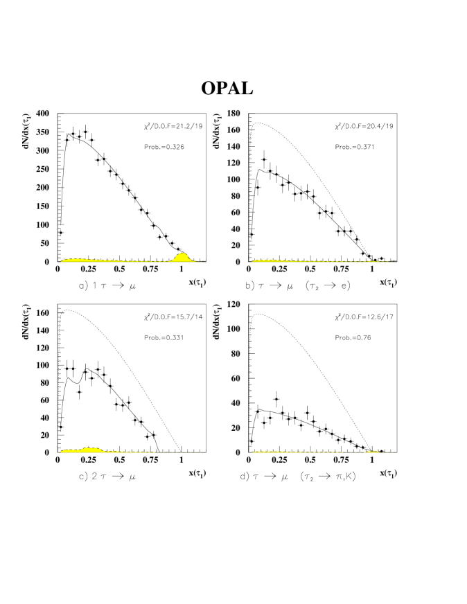
Figure 7.7: $x$ distributions for the $\tau$$\rightarrow$$\mu$$\bar{\nu}_{\mu}$$\nu_{\tau}$ decay channels and for various decays on the opposite side, compared with the theoretical predictions (solid lines) with all corrections included, taking the $\langle P_{\tau}\rangle$ value obtained from the global ML fit. The filled area represent the background part of the spectrum. The dotted lines are the uncorrected theoretical curves.

.

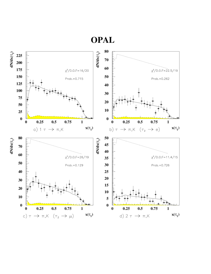
Figure 7.8: $x$ distributions for the $\tau$$\rightarrow$$\pi$(K)$\nu_{\tau}$ decay channels and for various decays on the opposite side, compared with the theoretical predictions (solid lines) with all corrections included, taking the $\langle P_{\tau}\rangle$ value obtained from the global ML fit. The filled area represent the background part of the spectrum. The dotted lines are the uncorrected theoretical curves.

.

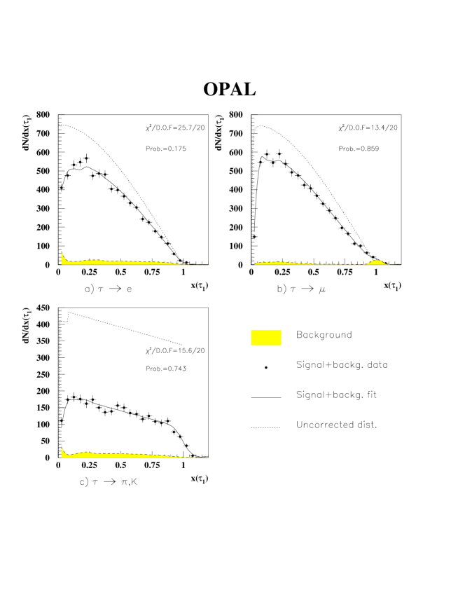
Figure 7.9: $x$ distributions for the $\tau$$\rightarrow$e$\bar{\nu}_{e}$$\nu_{\tau}$, $\tau$$\rightarrow$$\mu$$\bar{\nu}_{\mu}$$\nu_{\tau}$ and $\tau$$\rightarrow$$\pi$(K)$\nu_{\tau}$ decay channels, summing over all decays on the other side and compared with the theoretical predictions (solid lines) with all corrections included, taking the $\langle P_{\tau}\rangle$ value obtained from the global ML fit. The filled area represent the background part of the spectrum. The dotted lines are the uncorrected theoretical curves.

7.4.4 A $\chi^{2}$ fit consistency check

Another check of the ML fitting method is a $\chi^{2}$ fit of the $x$ distributions to a linear combination of the corrected theoretical curves for positive and negative helicity. The $\chi^{2}$ fit is meaningful only for the case where there is enough entries (at least 10) in each of the bins. Therefore, it was only applied to the case where just one tau was identified. The results which are listed in Table 7.4 are consistent with the ML fits listed in Table 7.3.

Decay Channel	$\langle P_{\tau}\rangle$
$\tau$$\rightarrow$e$\bar{\nu}_{e}$$\nu_{\tau}$	-21.1 $\pm$ 9.1
$\tau$$\rightarrow$$\mu$$\bar{\nu}_{\mu}$$\nu_{\tau}$	-4.2 $\pm$ 8.1
$\tau$$\rightarrow$$\pi$(K)$\nu_{\tau}$	-20.1 $\pm$ 4.6

Table 7.4: Tau polarization results calculated by $\chi^{2}$ fits to events where just one tau was identified.

7.4.5 Measurements of polarization as a function of $\cos\theta$

The results were also checked by dividing the $\cos\theta$ range into five intervals to determine the tau polarization in each of them separately using the ML fit. The results are plotted in Fig. 7.10. The solid line in the figure describes result of a $\chi^{2}$ fit of the tau polarization expected dependence on $\cos\theta$ (Eq. 4.27). The OPAL result for the Z⁰ peak $\mbox{\rm A${}_{FB}$}=1.2\%$  [6] is used (see Table 6.1). We obtained $(\mbox{$\langle P_{\tau}\rangle$}=-13.9\pm 2.9(stat.))\%$ and $\mbox{\rm A${}_{pol}^{FB}$}=(-10.8\pm 3.5(stat.))\%$, which is in excellent agreement with our nominal results. The fitted $\chi^{2}$ is 0.7 for 3 degrees of freedom and the correlation between $\langle P_{\tau}\rangle$ and A${}_{pol}^{FB}$ is 0.027.

7.4.6 A test of the A_FB influence

We also modified our fitting procedure allowing the seven A_FB values to be free parameters in the fit. They are consistent with the values which have been used in our standard fit, where the largest deviation is 1.8$\sigma$. Our statistical errors for A_FB are twice as large since we use only events in the barrel region and only those events where at least one tau was identified.

. .

Figure 7.10: Measured tau polarization results as function of $\cos\theta$. The solid line is our fit result (see text).

The corresponding results for $\langle P_{\tau}\rangle$ and A${}_{pol}^{FB}$ were $(-13.5\pm 2.9(stat.))\%$ and $(-10.9\pm 3.5(stat.))\%$ respectively, in an excellent agreement with our standard global fit values.

7.5 $\langle P_{\tau}\rangle$  and A${}_{pol}^{FB}$  from $\tau$$\rightarrow$$\rho$$\nu_{\tau}$  decays

In order to combine our results with those measured from the $\tau$$\rightarrow$$\rho$$\nu_{\tau}$  decays, we quote here the OPAL $\langle P_{\tau}\rangle$  and A${}_{pol}^{FB}$  measured from this decay channel. The two $\tau$$\rightarrow$$\rho$$\nu_{\tau}$ analyses done by OPAL has used a least squares fit to determine $\langle P_{\tau}\rangle_{\theta}$  in five $\cos\theta$ intervals, and than extracted the $\langle P_{\tau}\rangle$ and A${}_{pol}^{FB}$ parameters in a least squares fit of the $\langle P_{\tau}\rangle_{\theta}$ dependence on $\cos\theta$.

The results of these two $\tau$$\rightarrow$$\rho$$\nu_{\tau}$ analyses were combined, taking care of the fact that these two data sets have an overlap of 40%. The $\tau$$\rightarrow$$\rho$$\nu_{\tau}$ OPAL’s result is then:

$$\langle P_{\tau}\rangle = (-15.7\pm 2.4\pm 1.5)\%$$

A$${}_{pol}^{FB} = (-7.1\pm 2.8\pm 1.5)\%$$ (7.7)

It is worthwhile to know that there is no overlap between the events used in our analysis for $\tau$ decay to e, $\mu$ or $\pi$(K) and the events used by OPAL for the study of $\tau$$\rightarrow$$\rho$$\nu_{\tau}$. Specifically, in our analysis the events of the type $\ell$-$\rho$ (i.e. one tau decays to a lepton and the other tau decays to a $\rho$-meson) are discarded. On the other hand in the $\tau$$\rightarrow$$\rho$$\nu_{\tau}$ analyses events of the type $\pi$-$\rho$ were discarded. For events of the type $\rho$-$\rho$ each identified $\tau$$\rightarrow$$\rho$$\nu_{\tau}$ decay was weighted in the $\tau$$\rightarrow$$\rho$$\nu_{\tau}$ analyses by 0.5. Table 8.1 summarize the results of the $\mbox{$\tau$}\to$ e, $\mu$ or $\pi$(K) channels (ML fit), the results of the $\tau$$\rightarrow$$\rho$$\nu_{\tau}$ channel ($\chi^{2}$ fit) and the combined results.

7.6 Comparison With Previous Measurements

7.6.1 Previous determination of the Michel parameters

Muon decay has been used for determination of the structure of the charged weak interaction since the 1950’s [48, 68]. The Particle Data Group [69] values for the Michel parameters measured in muon decays are $\rho=0.7518\pm 0.0026$ [70], $\xi=1.0027\pm 0.0079\pm 0.0030$ [71], and $\delta=0.755\pm 0.009$ [72]. The ARGUS collaboration has recently published a measurement of two of the Michel parameters evaluated in leptonic tau decays [73]. For $\rho_{\mbox{$\tau$}\to\mu}$ and $\rho_{\mbox{$\tau$}\to e}$ they obtain from the $e$ and $\mu$ momentum spectra the values of $0.76\pm 0.07\pm 0.06$ and $0.79\pm 0.08\pm 0.06$ respectively. Assuming $\xi_{\mbox{$\tau$}\to\mu}=\xi_{\mbox{$\tau$}\to e}$ they have measured $\xi=0.90\pm 0.15\pm 0.10$. The ALEPH collaboration have used the correlation in $\tau$ pairs where both $\tau$’s decay into hadrons ($\pi$ or $\rho$) to measure $\xi_{had}$. Their values are [74]: $\xi_{\pi}=0.95\pm 0.11\pm 0.05$, $\xi_{\rho}=1.03\pm 0.11\pm 0.05$ or assuming $\xi_{\pi}=\xi_{\rho}$ they obtained $0.99\pm 0.07\pm 0.04$.

$\tau$ decay	Exp.	$\langle P_{\tau}\rangle$ (%)	A${}_{pol}^{FB}$ (%)
$\tau$$\rightarrow$e$\bar{\nu}_{e}$$\nu_{\tau}$	L3	-12.7$\pm$9.7$\pm$6.2	–
	DELPHI	-12$\pm$27$\pm$8	–
	ALEPH	-22.5$\pm$8.5$\pm$4.5	–
	OPAL 1	20$\pm$13$\pm$8	-16$\pm$19
	OPAL 2	-8.5 $\pm$ 5.8$\pm$4.5	-10.4 $\pm$ 6.6$\pm$1.3
$\tau$$\rightarrow$$\mu$$\bar{\nu}_{\mu}$$\nu_{\tau}$	L3	-2.0$\pm$ 10.1$\pm$5.5	–
	DELPHI	-5$\pm$18$\pm$7	–
	ALEPH	-15.4$\pm$6.5$\pm$2.9	–
	OPAL 1	-17$\pm$16$\pm$10	-88$\pm$22
	OPAL 2	-8.0 $\pm$ 5.4$\pm$3.3	-10.1 $\pm$ 6.2$\pm$1.3
$\tau$$\rightarrow$$\pi$(K)$\nu_{\tau}$	L3	-14.8$\pm$ 9.7$\pm$6.2	–
	DELPHI	-35$\pm$11$\pm$7	–
	ALEPH	-13.3$\pm$3.1$\pm$1.8	–
	OPAL 1	-8$\pm$10$\pm$7	-34$\pm$16
	OPAL 2	-14.3 $\pm$ 3.7$\pm$3.0	-10.9 $\pm$ 4.5$\pm$0.8
All	L3	-13.2$\pm$ 2.6$\pm$2.1	–
	DELPHI	-24$\pm$7	–
	ALEPH	-14.3$\pm$2.3	-9$\pm$2
	OPAL 1	-9.7$\pm$8.4	-22$\pm$10
	OPAL 2	-11.3 $\pm$ 3.3	-10.6 $\pm$ 3.3

Table 7.5: The LEP experiments $\tau$ polarization published results for the $\tau$$\rightarrow$e$\bar{\nu}_{e}$$\nu_{\tau}$,$\tau$$\rightarrow$$\mu$$\bar{\nu}_{\mu}$$\nu_{\tau}$ and $\tau$$\rightarrow$$\pi$(K)$\nu_{\tau}$ channels. When two errors are quoted the first is the statistical and second is the systematic error, when one error is quoted it is the combined statistical and systematic error. The L3 [10] and ALEPH [11] published the study of 1990-1991 data using five decay channels of $\tau$ (e, $\mu$, $\pi(K)$, $\rho$ and $a_{1}$). DELPHI’s publication [9] is based on the analysis of four decay channels (e, $\mu$, $\pi(K)$ and $\rho$) from the years 1990-1991. The OPAL 1 is the OPAL first publication [7] based on the analysis of three decay channels (e, $\mu$ and $\pi(K)$) during 1990. OPAL 2, is the present analysis using 1990-1992 e, $\mu$ and $\pi(K)$ decay channels. Note that for the comparison with the other numbers the individual results quoted assume, incorrectly, that there are no correlations between the taus. These correlations are fully taken into account in the global ML fit result.

7.6.2 Results to compare with other measurements

In the analyses published by OPAL in the past [7] and by other LEP collaborations [9]-[11], one did not look at the whole $\tau$-pair event. Instead, one did consider each decay separately, ignoring the opposite side. In order to be able to compare our results with those of other analyses, we repeated our ML fit adopting their policy. For that, we had to recalculate those corrections depending on the whole event, such as $\tau$-pair selection efficiencies and non-tau background. Each event, where both $\tau$’s were identified, was handled as two independent events. In Table 7.5 we list the results for each decay channel separately. One should note, however, that the results for the $\tau$$\rightarrow$e$\bar{\nu}_{e}$$\nu_{\tau}$, $\tau$$\rightarrow$$\mu$$\bar{\nu}_{\mu}$$\nu_{\tau}$ and $\tau$$\rightarrow$$\pi$(K)$\nu_{\tau}$ decays in this table cannot be interpreted as independent polarization measurements because the same tau-pair event can contribute to two channels.

7.6.3 LEP tau polarization results

The following Table 7.6, presents the up to date but preliminary $\langle P_{\tau}\rangle$ and A${}_{pol}^{FB}$ results of all other 3 LEP detectors presented at the La Thuile and Moriond Conferences in March 1994  [67]. The OPAL figures are those of the present analysis combined with the $\tau$$\rightarrow$$\rho$$\nu_{\tau}$ figures [18]. In averaging the results we repeat the procedure discussed by the LEP tau polarization group in Ref. [67]. Three common effects, which affect all the tau decay mode equally, were taken into account:

• A dependence of the results on $E_{cm}$ due to a direct $\gamma$ and $\gamma$ - Z⁰ interference contributions to the Z⁰ intermediate state. These were corrected so that the results quoted correspond to $\mbox{$E_{cm}$}=M_{Z}$.

• Electromagnetic initial and final state radiative corrections.

• Born level mass terms leading to helicity flip configurations.

As shown by the theoretical calculations in Refs.  [37, 56, 65, 75] the combined effect of these three is to reduce the strength of the measured $\langle P_{\tau}\rangle$ (A${}_{pol}^{FB}$) by about 0.3% (0.2%). Therefore the experiments results (including ours) were corrected by adding this amount to the measured $\langle P_{\tau}\rangle$ and A${}_{pol}^{FB}$. The four experiments results were combined without extracting a common systematic error. The $\chi^{2}/D.O.F.$ for the average is 2.2/3 and 1.7/3 for $\langle P_{\tau}\rangle$ and A${}_{pol}^{FB}$ respectively. The results of the four experiments and their average are summarized in Fig. 7.11.

Experiment	$\langle P_{\tau}\rangle$	A${}_{pol}^{FB}$
	(%)	(%)
OPAL	$-15.3\pm 2.3$	$-9.2\pm 2.4$
L3	$-17.4\pm 2.1$	$-9.8\pm 1.9$
DELPHI	$-15.4\pm 2.3$	$-6.1\pm 2.5$
ALEPH	$-13.7\pm 1.4$	$-9.5\pm 1.3$
LEP Average	$-15.0\pm 0.9$	$-9.1\pm 0.9$

Table 7.6: LEP results for  $\langle P_{\tau}\rangle$ and A${}_{pol}^{FB}$. The OPAL figures are the updated results where the figures of all other three experiments are preliminary results presented at MORIOND 94.

.

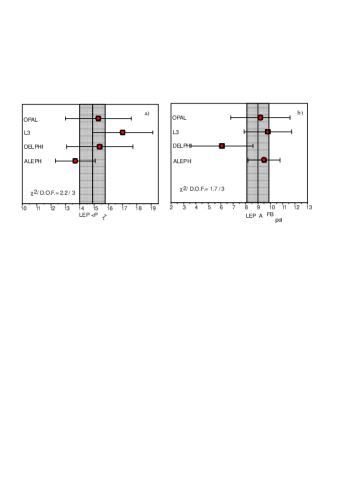
Figure 7.11: LEP results for  $\langle P_{\tau}\rangle$ and A${}_{pol}^{FB}$. The ALEPH, DELPHI and L3 are preliminary results given at the MORIOND 94 conference, whereas the OPAL figures are the updated results sent for publication. The shaded areas are the averages of the 4 experiments.

Chapter 8 Summary

We have measured the average tau polarization and its forward backward asymmetry using the tau decay channels $\tau$$\rightarrow$e$\bar{\nu}_{e}$$\nu_{\tau}$, $\tau$$\rightarrow$$\mu$$\bar{\nu}_{\mu}$$\nu_{\tau}$ and $\tau$$\rightarrow$$\pi$(K)$\nu_{\tau}$. The results of these measurements (taking into account all corrections) are

$$\langle P_{\tau}\rangle = (-13.5\pm 2.9\pm 2.2)\%$$

A$${}_{pol}^{FB} = (-11.0\pm 3.5\pm 0.5)\%$$ (8.1)

where the first error is statistical and the second systematic. Our Maximum Likelihood fit method takes into account correlations between the decay distributions of the $\tau^{-}$ and the $\tau^{+}$ in the same event due to their opposite helicity. The theoretical expectation had to be corrected for radiative effects, detector resolution, efficiencies of $\tau$-pair selection and tau decay identification, and background originating from other $\tau$ channels and non-$\tau$ events. These correction were calculated from Monte Carlo events and whenever possible, checked with control measured data.

A summary of the measurements from all channels is presented in Table 8.1.

Decay Channel	$\langle P_{\tau}\rangle$	A${}_{pol}^{FB}$
	(%)	(%)
$\mbox{\mbox{$\tau$}\mbox{$\rightarrow$}\mbox{\rm e}\mbox{$\bar{\nu}_{e}$}\mbox{$\nu_{\tau}$}},\mu\bar{\nu}_{\mu}\nu_{\mbox{$\tau$}},\pi(K)\nu_{\mbox{$\tau$}}$ present analysis	-13.5$\pm$2.9$\pm$2.2	-11.0$\pm$3.5$\pm$0.5
OPAL $\tau$$\rightarrow$$\rho$$\nu_{\tau}$	-15.7$\pm$2.4$\pm$1.5	-7.1$\pm$2.8$\pm$1.5
OPAL combined results	-14.9$\pm$1.9$\pm$1.3	-8.9$\pm$2.2$\pm$0.9

Table 8.1: OPAL combined $\tau$ polarization results.

The results are quoted for $\sqrt{s}=m_{Z}$. A very small correction ($1\%$ of the $\langle P_{\tau}\rangle$), which takes into account the fact that some data was collected off the peak of the Z⁰ resonance, is made. Our final result, combined with the OPAL $\tau$$\rightarrow$$\rho$$\nu_{\tau}$ results are:

$$\mbox{$\langle P_{\tau}\rangle$}= -\mbox{${\cal A}_{\tau}$}= (-14.9\pm 1.9\pm 1.3)\%$$

$$\mbox{\rm A${}_{pol}^{FB}$}= -\frac{3}{4}\mbox{${\cal A}_{e}$}= (-8.9\pm 2.2\pm 0.9)\%.$$ (8.2)

Following these results we obtain:

$$\mbox{${\cal A}_{\tau}$}= \frac{2v_{\tau}a_{\tau}}{v_{\tau}^{2}+a_{\tau}^{2}}= 0.153\pm 0.023$$ (8.3)

$$\mbox{${\cal A}_{e}$}= \frac{2v_{e}a_{e}}{v_{e}^{2}+a_{e}^{2}}= 0.122\pm 0.032$$

where the errors include both statistical and systematic uncertainties. These are already corrected, (using ZFITTER  [75]), for the contribution of the intermediate $\gamma$, $\gamma$-Z⁰ interference and other photonic radiative corrections. Therefore they can be interpreted in terms of the vector and axial-vector couplings within the improved Born approximation. In the context of the SM ${\cal A}_{\tau}$ and ${\cal A}_{e}$ yield a measured values for the coupling ratios of

$$v_{\tau}/a_{\tau} = 0.077\pm 0.012$$ (8.4)

$$v_{e}/a_{e} = 0.062\pm 0.016$$

where as before the error includes both statistical and systematic contributions.

These measured values of $\langle P_{\tau}\rangle$ and A${}_{pol}^{FB}$ correspond to the following values of $\sin^{2}\theta_{W}^{\mbox{\small\it eff}}$ (see Eq.  4.42):

$$\mbox{$\sin^{2}\theta_{W}^{\mbox{\small\it eff}}$}(\mbox{$\langle P_{\tau}\rangle$}) = 0.2308\pm 0.0030$$ (8.5)

$$\mbox{$\sin^{2}\theta_{W}^{\mbox{\small\it eff}}$}(\mbox{\rm A${}_{pol}^{FB}$}) = 0.2345\pm 0.0040.$$

These values are in a good agreement with the hypothesis of lepton universality. Therefore they can be averaged (with $\mbox{$\chi^{2}$}=0.56$) to give ,

$$v/a = 0.072\pm 0.010$$ (8.6)

$$\sin^{2}\theta_{W}^{\mbox{\small\it eff}} = 0.2331\pm 0.0023$$

Fig. 8.1 presents the result of various determinations of $\sin^{2}\theta_{W}^{\mbox{\small\it eff}}$measured at LEP and SLD. These were calculated from the observed forward backward asymmetries of leptons ($\mbox{\rm A${}_{FB}$}(\ell\ell))$ and quark pairs ($\mbox{\rm A${}_{FB}$}(b\bar{b}),\;\;\mbox{\rm A${}_{FB}$}(c\bar{c})$ and $\langle Q_{FB}\rangle$- the inclusive forward backward asymmetry of negative quarks), the tau polarization and its forward backward asymmetry.

The figures of the charge asymmetries are those which were presented as LEP results in the Moriond 94 conference [76]. The results given for the $\langle P_{\tau}\rangle$ and A${}_{pol}^{FB}$ are the modified OPAL numbers using the results of the present work. The obtained LEP average (with $\mbox{$\chi^{2}/D.O.F.$}=5.9/5$) is

$$\mbox{$\sin^{2}\theta_{W}^{\mbox{\small\it eff}}$}(LEP)=0.2322\pm 0.0004$$

For a comparison, also the SLD value of $\sin^{2}\theta_{W}^{\mbox{\small\it eff}}$ derived from their measurement of the left-right asymmetry, $A_{LR}$ is given. This asymmetry is defined in a fully polarized electrons beam as

$$A_{LR}=\frac{\sigma_{L}-\sigma_{R}}{\sigma_{L}+\sigma_{R}}=\mbox{${\cal A}_{e}$}$$ (8.7)

which means that it probes the same couplings as the A${}_{pol}^{FB}$. One can see from Fig. 8.1 that while there is a good agreement betwen all LEP results, the present SLD value for $\sin^{2}\theta_{W}^{\mbox{\small\it eff}}$ [77] is shifted from the LEP numbers. Therefore as expected, the $\chi^{2}$ obtained when combining the measured weak mixing angle of LEP and SLD there is no good agreement ($\mbox{$\chi^{2}/D.O.F.$}=13.3/6$). The average value being

$$\mbox{$\sin^{2}\theta_{W}^{\mbox{\small\it eff}}$}(LEP+SLD)=0.2317\pm 0.0003$$

.

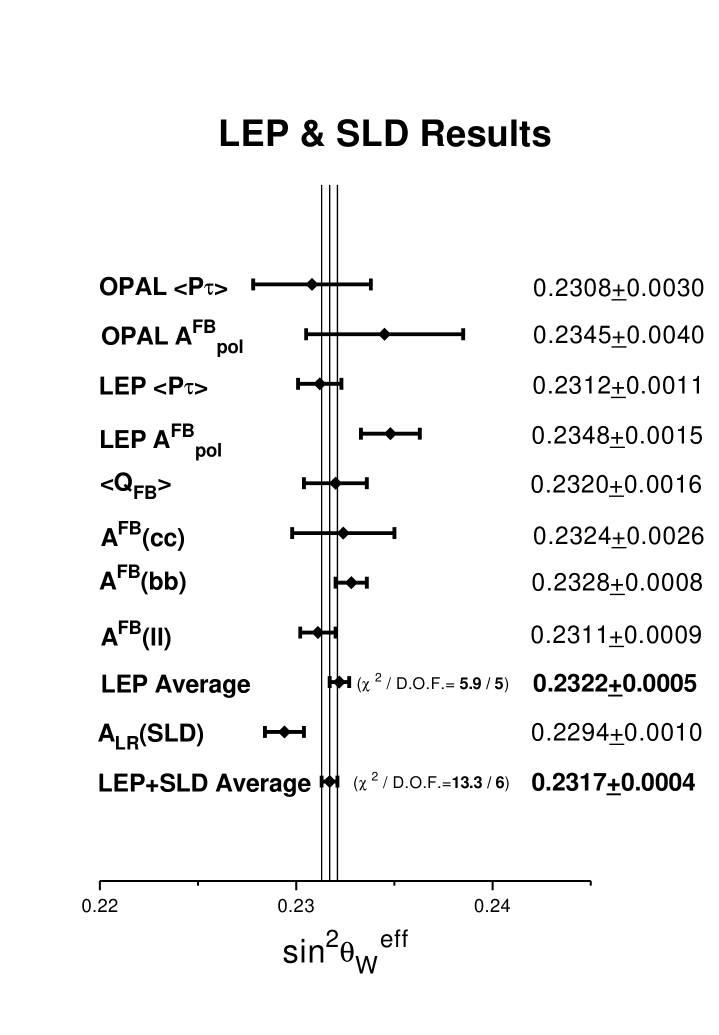
Figure 8.1: Comparison of several determinations of the weak mixing angle from asymmetries as was presented in the MORIOND 94 conference. The values of LEP were modified using the results of the present analysis. Combined results of the LEP experiments and a combined LEP-SLD results are obtained as weighted averages assuming no correlations.

Bibliography

- [1] S. L. Glashow, Nucl. Phys. 22 (1961) 579.
- [2] S. Weinberg, Phys. Rev. Lett. 19 (1967) 1264.
- [3] A. Salam, in proceeding of the Eight Nobel Symposium, on Elementary Particle Theory, ed. N. Svartholm (1968) 367.
- [4] S. Jadach and Z. Wa̧s in ”The Polarization Measurement”, Z physics at LEP1, CERN Yellow Report 89-08, eds. G. Altarelli et al., Vol. 1 (1989) p. 235, and an update of august 1990.
- [5] M. Consoli, W. Hollik and F. Jegerlehner in Z Physics at LEP1, CERN 89-08, ed. G. Altarelli et al., Vol. 1 (1989) 7.
-
[6]
OPAL Collaboration:
M.Z. Akrawy et al., Phys. Lett. B240 (1990) 497.
G. Alexander et al., Z. Phys. C52 (1991) 175.
R. Akers et al., Z. Phys. C61 (1994) 19. - [7] OPAL Collaboration, G. Alexander et al., Phys. Lett. B266 (1991) 201.
- [8] ALEPH Collaboration, D. Decamp et al., Phys. Lett. B265 (1991) 430.
- [9] DELPHI Collaboration, P. Abreu et al., Z. Phys. C55 (1992) 555.
- [10] L3 Collaboration, O. Adriani et al., Phys. Lett. B294 (1992) 466.
- [11] ALEPH Collaboration, D. Buskulic et al., Z. Phys. C59 (1993) 369.
- [12] DELPHI Collaboration, contribution to XVI International Symposium on Lepton-Photon Interactions, Cornell University, August 1993.
- [13] L3 Collaboration, contribution to the Int. Europhysics Conf. on High Energy Physics, Marseille, July 1993.
- [14] A. Beck, ”-Polarization and its Forward-Backward Asymmetry From The channel Using Dedicated Clustering”, OPAL technical note TN203 (1994).
- [15] M. Rosvick, ”Results of the Victoria analysis”, OPAL technical note TN142 (1993).
- [16] G. Bella and E. Etzion, ”Analysis of the Polarization and its Forward-Backward Asymmetry Using a Global Fit Method”, OPAL technical note TN202 (1994).
- [17] A. Beck,G. Bella,E. Etzion,M. Roney,M. Rosvick and M. Sasaki, ”Measurement of the tau lepton polarization and its forward-backwad asymmetry at LEP”, OPAL Physics Note, PN126 (1994).
- [18] OPAL Collaboration, R. Akers et al., ”Measurement of the Tau Lepton Polarization and its Forward-Backward Asymmetry from Z0 Decays”, CERN-PPE/94-120 (1994), submitted to Z. Phys. C .
- [19] P. Schmuser, ”Basic course on accelerator optics”, CERN acceleration school, General accelerator physics Aarhus Denmark, Sep. 86, ed. S. Turner CERN 87-10, (1987) 1.
- [20] A. Hofmann, Nucl. Phys. B3 (1988) 511.
- [21] J. J. Tresher, ”LEP: machine and experiment”, XXIV International conference on High energy Physics, eds. R. Kotthaus and J. H. Kuhn, Munich, Germany, (1988) 387.
- [22] ”Large Electron Positron storage ring - Technical notebook” CERN (1988) 1.
- [23] OPAL Technical Proposal, CERN/LEPC/83-4.
- [24] OPAL Collaboration, K. Ahmet et al., Nucl. Inst. and Meth. A305 (1991) 275.
- [25] OPAL Collaboration, M.Z. Akrawy et al., Phys. Lett. B231 (1989) 530.
- [26] D.G. Charlton et al., Nucl. Inst. and Meth. A325 (1993) 129 .
- [27] R. Brun, M. Goossens and J. Zoll, ZEBRA Dynamic Data Structure and Memory Manager, Program Library, CERN.
- [28] A. Zee, ”Unity of forces in the universe”, World Scientific (1982).
- [29] Mark II at SLAC and all four LEP detectors at CERN have measured this number of families (with ). See for example the OPAL publication ref. [25].
- [30] B.C. Barish and R. Stroynowski, Phys. Rep. 157 (1988) 1.
- [31] Y. S. Tsai, Phys. Rev. D4 (1971) 2821.
- [32] D. A. Dicus, Phys. Rev. D8 (1973) 890.
- [33] R. Koniuk, R. Leroux, N. Isgur, Phys. Rev. D17 (1978) 2915.
- [34] J.E. Augustin, ”Use of Hadronic Decay to Study Polarization Near Pole at LEP”, ECFA/LEP 29, Proceeding of the LEP summer study, CERN 79-01, vol. 2 (1979) 499.
- [35] G. Goggy, ”Study of Heavy Lepton Polarization in Annihilation at the Pole”, ECFA/LEP 2, Proceeding of the LEP summer study, CERN 79-01, vol. 2 (1979) 483.
- [36] G. Goggy, Letters al Nuovo Cimento , Vol 24 (1979) 2.
- [37] S. Jadach and Z. Wa̧s, Acta Physica Polonica, Vol B15 (1984) 1151.
- [38] D. Dorfan, ”Polarization Experiments without Polarized Beams: ”, SLAC PUB. 3407 (1984).
- [39] J. Chauveau, ”Testing the Standard Model by Measuring the Helicity at ”, Physics at LEP, eds. J. Elis R. Pecci, CERN report 86-02 (1986).
- [40] G. Burgers and W. Hollik, ”The shape and size of Z resonance”, Polarization at LEP, CERN report 88-06, eds. G. Alexander et al., CERN, Geneva (1988) 136.
- [41] K. Hagiwara, A.D. Martin, D. Zeppenfeld, Phys. Lett. B235 (1990).
- [42] E. Etzion, ” Measurements in the Channel Using Decay”, OPAL technical note TN031 (1991), and M.Sc. thesis, Tel Aviv University (June 1991).
- [43] G. Alexander, C. Milstène, W. Hollik, Z. Phys. C52 (1991) 283.
- [44] J. Ellis and M.K. Gaillard, CERN 76-18 (1976) p21.
- [45] see e.g. F. Halzen, A. D. Martin, Quarks & leptons, Wiley-Interscience (1984).
- [46] W. Fetscher, H.J. Gerber, K.F. Johnson, Phys. Lett. B173 (1986) 102.
- [47] P. Privitera, Phys. Lett. B288 (1992) 227.
- [48] L. Michel, Proc. Phys. Soc. A63 (1950) 514.
- [49] OPAL Collaboration, contribution to the Int. Europhys. conf. on High Energy Physics, Marseille, July 1993.
- [50] A. Gulotvin, ”New Determination of Michel Parameters in Leptonic Decays”, Contribution of the Second Workshop on Tau Lepton Physics, Ohio (September 1992).
- [51] G. Alexander, G. Bella and E. Etzion, ”The statistical Errors of -Asymmetries and their Correlations”, OPAL Technical Note TN062 (1992) .
- [52] G. Bella, ”The Weight Ratio Method and its Application to Identify -Decay Modes”, OPAL Technical Note TN058 (1992).
- [53] The Tau Platform (TP) Manual, Version 1.02.
- [54] J. Allison et al., Nucl. Inst. and Meth. A317 (1992) 47.
-
[55]
J. Allison et al., Comp. Phys. Comm. 47 (1987) 55;
R. Brun, F. Bruyant, M. Maire, A. C. McPherson, and P. Zanarini, GEANT3, CERN DD/EE/84-1 (1987). -
[56]
S. Jadach, B.F.L Ward and Z. Wa̧s, Comp. Phys. Comm. 66 (1991) 276;
S. Jadach, J.H. Kühn and Z. Wa̧s, Comp. Phys. Comm. 64 (1991) 275. -
[57]
T. Sjöstrand, Comp. Phys. Comm. 39 (1986) 347;
M. Bengtsson and T. Sjöstrand, Comp. Phys. Comm. 43 (1987) 367;
M. Bengtsson and T. Sjöstrand, Nucl. Phys. B289 (1987) 810 (JETSET). - [58] OPAL Collaboration, M. Z. Akrawy et al., Z. Phys. C47 (1990) 505.
-
[59]
M. Bohm, A. Denner and W. Hollik, Nucl. Phys. B304
(1988) 687;
F. A. Berends, R. Kleiss and W. Hollik, Nucl. Phys. B304 (1988) 712. -
[60]
R. Battacharya, J. Smith and G. Grammer, Phys. Rev. D15 (1977) 3267;
J. Smith, J. A. M. Vermaseren and G. Grammer, Phys. Rev. D15 (1977) 3280. - [61] OPAL Collaboration, G. Alexander et al., Z. Phys. C52 (1991) 175.
- [62] J. Clayton, private communication.
- [63] OPAL Collaboration, Phys. Lett. B328 (1994) 207.
- [64] G. Alexander and E. Etzion, ”Some Aspects Concerning the Selection of Events”, CERN August 1989.
- [65] E. Barberio, B. van Eijk and Z. Wa̧s, Comp. Phys. Comm. 66 (1991) 115.
- [66] M. Sasaki, ”Improved Extraction Method Used for Tau Polarization Measurement”, OPAL Technical Note TN192 (1993).
- [67] J. Harton et al., Tau Polarization Group of LEP, ”Combining the LEP tau polarisation results”, LEPTAU 94-01 and OPAL technical note TN226 (1994).
- [68] W. Fetscher, H.J. Gerber and K.F. Johnson, Phys. Lett. B173 (1986) 102.
- [69] Review of Particles Properties, K. Hikasa et al., (Partcle Data Group), Phys. Rev. D45 (1992) Part II.
- [70] S. E. Derenzo, Phys. Rev. 181 (1969) 1854.
- [71] I. Beltrami et al., Phys. Lett. B194 (1987) 326.
- [72] B. Bulke et al., Phys. Rev. D37 (1988) 587.
- [73] ARGUS Collaboration, Albrecht et al., Phys. Lett. B324 (121), 1994.
- [74] ALEPH Collaboration, D. Buskulic, et al., Phys. Lett. B321 (1994) 168.
- [75] D. Bardin et al., CERN-TH. 6443/92 (1992) (ZFITTER).
- [76] The LEP Electroweak Working Group, ”Updated Parameters of the Z0 Resonance from Combined Preliminary Data of the LEP Experiments”, LEPEWWG/94-01 and OPAL Technical Note TN235 (1994).
- [77] SLD Collaboration, K. Abe et al., ”Precise Measurement of the Left-Right Cross Section Asymmetry in Z Boson Production by Collisions” SLCA-PUB 6456 (1994), submitted to Phys. Rev. Lett.