PHYSICS PROSPECTS
— WHY DO WE WANT A LINEAR COLLIDER? –

Abstract

The need to understand physics of electroweak symmetry breaking is reviewed. An electron positron linear collider will play crucial roles in that respect. It is discussed how the LHC and a linear collider need each other to understand symmetry breaking mechanism unambiguously. Two popular scenarios, supersymmetry and technicolor-like models, are used to demonstrate this point.

1 Introduction

Now the long-awaited top quark is discovered.

I have been trying to tell my non-physicists friends how significant this result is. Some told me back before I began explanations,

“Oh, yeah, I read the story in The New York Times. I thought particle physics is over now.”

Everbody in this audience knows the impression my friend got from the newspaper article is wrong. But how wrong? I believe it is useful to start my talk by discussing where we are now. Then it becomes clearer where we are heading, and what experimental facilities we need to achieve our goals.

2 Where are we?

As everybody in this audience knows, there are (at least) two important and exciting progress in particle physics in recent years. The first one is of course the discovery of the top quark. The indication of its existence goes back to the discovery of $\tau$-lepton in 1975 for which Martin Perl was awarded the 1995 Nobel Prize in Physics. The existence of the third generation lepton, combined with the theoretical requirement of the anomaly cancellation, implies there must exist bottom and top quarks. The bottom quark was discovered by a group led by Leon Lederman in 1976. This was the start of the long search for the top quark. The electron positron colliders, PEP, PETRA, and TRISTAN established that the bottom quark has an isospin $g_{A}=-1/2$, which indicated the bottom quark has (at least) one partner with charge $2/3$. The precision electroweak measurements at LEP and SLC determined the mass range of the top quark to be $m_{t}=169^{+23}_{-27}$ GeV (PDG 94) indirectly. And finally, in year 1995, the long sought-after particle was discovered by CDF and D0 experiments at Fermilab, Tevatron. This was a great confirmation of our current understanding in particle physics based on SU(2)$\times$U(1) gauge theory.

Another important progress was that the universality of weak interactions was established at an extremely high precision. The ratio of strengths of the charged current interactions (CC) of quarks and leptons are known to be

$$\frac{\mbox{strengh of CC for up quark}}{\mbox{strengh of CC for $e$ and $\mu$}}=|V_{ud}|^{2}+|V_{us}|^{2}+|V_{ub}|^{2}=0.9983\pm 0.0015,$$ (1)

which supports strongly a universal strengh. More remarkably, experiments at LEP and SLC supplied many independent measurements of the strengh of weak neutral current, $\sin^{2}\theta_{W}$, which are consistent with each other with a healthy fluctuation (see Fig. 1).

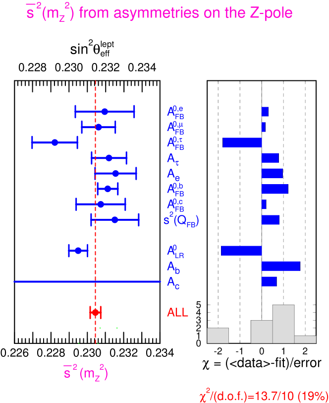
Figure 1: A plot showing the universality of $\sin^{2}\theta_{W}$ in many different experimental observables (asymmetries) from experiments at LEP and SLC. Made by S. Matsumoto.

The universality of both charged and neutral weak interactions, combined with the discovery of predicted top quark, strongly suggests that the weak interactions are described by a gauge theory. Or in other words, the $W^{\pm}$ and $Z^{0}$ bosons are gauge bosons. This is a natural analogue of the fact that other known universal forces, namely gravity, which acts univerally on all bodies (equivalence principle), and electromagnetism, which gives universal Coulomb force which does not depend on the properties of matter but only on their electric charges, are described by gauge theories. In fact, the universality was the main motivation for Glashow to describe the weak interactions by his SU(2)$\times$U(1) gauge theory, or electroweak theory.

However, here we encounter a contradiction. Other known gauge forces, gravity and electromagnetism, are known to be long-ranged. For instance, the range of electromagnetism is known to be larger than 1 kpc from the fact that the galactic magnetic field extends over a distance of this order of magnitude. On the other hand, the weak forces are very short-ranged; they do not act beyond a distance of $10^{-16}$ cm.

The short-rangedness of weak interactions tells us that the electroweak gauge symmetry has to be broken. The “vacuum” is filled with a condensate which is electrically neutral, but feels weak forces. Since the condensate is electrically neutral, photon can freely travel in the “vacuum” without knowing there exists a condensate. On the other hand, the carriers of weak forces, $W^{\pm}$ and $Z^{0}$ bosons, cannot travel freely in the “vacuum” because their motion is disturbed by the condenstate which feels the weak forces. Because of this disturbance due to the condensate, $W^{\pm}$ and $Z^{0}$ bosons cannot travel far, and the weak interactions become short-ranged.

In the Standard Model, the condensate is assumed to be a spinless boson which acquires a vacuum expectation value. In order to generate this condensate, one introduces a potential for the spinless boson and assumes it has a double-well form such that the minimum of the potential lies where the boson has a non-vanishing value. However, this “explanation” leaves many questions open. First of all, why such a spinless boson exists, while we have not seen any elementary spinless bosons in nature yet. Even if we accept the existence of such a spinless boson, it is mysterious why it has such a special form of the potential which is designed to generate a non-vanishing vacuum expectation value. Furthermore, we know that the masses of elementary fermions, leptons and quarks, vary between almost six orders of magnitudes. The “explanation” of this diversity in the Standard Model is that the top quark, the heavest particle, interacts with the condenstate strongly and its motion is substantially disturbed as the $W^{\pm}$ and $Z^{0}$ bosons, while the electron, the lightest charged particle, interacts only very weekly with the condensate so that it does little harm to the motion of electrons. It is left completely unexplained why the quarks and leptons interact with the condensate with so different strengths.

Because of this unsatisfactory nature, the Standard Model cannot be the whole story of nature. A true theory of the electroweak symmetry breaking, the mechanism which makes the weak interactions short-ranged, must explain why it is broken. I believe this is an experimental question which has to be answered by studing the properties of $W^{\pm}$, $Z^{0}$ bosons and search for new phenomena below TeV scale. Despite the efforts by both our experimental and theoretical colleagues for more than two decades, we have little clue on this point. The next generation experiments have to planned so that they will be able to give us clues to answer this question.

Now what kinds of experimental facilities are needed to explore the physics of electroweak symmetry breaking? To discuss this point, I use two popular scenarios, supersymmetry and technicolor, as representative models. Even though we probably have not exhausted all theoretical possibilities to explain the electroweak symmetry breaking, an experiment cannot cover a scenario which we could not think of so far if it cannot cover already-known scenarios. Therefore, future facilities have to be designed to cover at least these two scenarios of electroweak symmetry breaking.

In Table 1, I listed “explanations” to various questions in the Standard Model in both scenarios. As one can easily see, both of them predict very rich phenomena at TeV scale. Moreover, both of them leave further fundamental questions to physics at yet higher energies which are very distinct. Therefore, we will obtain very useful clues to the physics much above TeV scale once we understand the physics of electroweak symmetry breaking. TeV scale machines will give us hints on physics at much higher energy scales.

Table 1: “Explanations” given to basic questions on physics of electroweak symmetry breaking in various theory scenarios. The contents in this table are meant to be examples, rather than representative ones. Especially those on fermion masses are controversial.

	Standard Model	Supersymmetry	Technicolor
Existence	Only scalar boson	Just one of many	No Higgs boson.
of Higgs	introduced just to	scalar bosons,	There are only fermi-
boson	break EW symmetry	nothing special	ons and gauge bosons.
Why electro-	by an	$m^{2}$ driven negative	new strong
weak symmetry	ad hoc choice	dynamically by top	force binds fermions
is broken	$m^{2}<0$	quark Yukawa coupling	to let them condense
pattern of	choose size of	sequential breaking of	further new
quark, lepton	Yukawa couplings	flavor symmetry just	forces at 1 to 1000
masses	to reproduce them	below the Planck scale	TeV scales
new		superpartners of	resonances at 1–10
phenomena	only a Higgs boson	all known particles	TeV, PNGBs and new
		below TeV scale	fermions at 0.1–1 TeV

As clear from the Table 1, physics of electroweak symmetry breaking is necessarily rich and complex. The challenge in designing the next generation experiments is to disentangle such complex signatures. In later sections, I discuss the case of supersymmetry scenario and “techicolor-like” scenario to see how well we can understand physics of electroweak symmetry breaking at the LHC and a possible future electron positron linear collider. It will be argued that both types of colliders are necessary to understand rich physics of electroweak symmetry breaking unambiguously; they play different roles, and work together leading us to decide yet-further future direction of the field.

3 Light Higgs and supersymmetry case

Let me take the Minimal Supersymmetric Standard Model (MSSM) as an example below. There are five Higgs bosons in this model,

$$h^{0},H^{0},A^{0},H^{+},H^{-},$$

and the mass of the lightest neutral scalar $h^{0}$ has to be smaller than $m_{h^{0}}\mathrel{\mathchoice{\lower 3.0pt\vbox{\halign{$\m@th\displaystyle\hfill#\hfil$\cr<\crcr\sim\crcr}}}{\lower 3.0pt\vbox{\halign{$\m@th\textstyle\hfill#\hfil$\cr<\crcr\sim\crcr}}}{\lower 3.0pt\vbox{\halign{$\m@th\scriptstyle\hfill#\hfil$\cr<\crcr\sim\crcr}}}{\lower 3.0pt\vbox{\halign{$\m@th\scriptscriptstyle\hfill#\hfil$\cr<\crcr\sim\crcr}}}}130$ GeV including radiative corrections.[1] It decays primarily into $b\bar{b}$, and into $\gamma\gamma$ with a branching fraction of $\sim 10^{-3}$ or less.

The LHC will see the signal of a light neutral scalar decaying into $\gamma\gamma$ with an impressive capability even in the high luminosity environment (Fig. 2). The ATLAS and CMS experiments will discover the Standard Model Higgs boson over the entire mass range above LEP2 reach up to 600 GeV or so. The $\gamma\gamma$ rate is in general lower in the Minimal Supersymmetric Standard Model than in the Standard Model, but still they will cover most of the parameter space. This is a highly significant capability of these experiments.

Figure 2: Expected $h\rightarrow\gamma\gamma$ signal for the Standard Model Higgs $m_{h}=120$ GeV, combined with the prompt $\gamma\gamma$ background, assuming an integrated luminosity of $10^{5}$ pb^-1. Taken from ATLAS TDR.[3]

However I still have a worry if there were only LHC and no electron positron collider. It is not the fact that there remains a hole in the MSSM parameter space (Fig. 3), as some people emphasize. This may be filled by running experiments for 3 years at high luminosity and combine two experiments.[5] My worry is it is not clear what we will learn either by seeing this signal or by not seeing it.

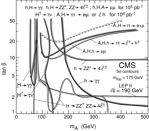
Figure 3: The coverage of the MSSM Higgs parameter space by CMS experiment.[4]

Suppose we will see a peak in $\gamma\gamma$ invariant mass distribution. I worry that it may not decide what is responsible for electroweak symmetry breaking. Let me first present a toy example of a model which has nothing to do with electroweak symmetry breaking but gives exactly the same signature and rate. This model has a new quark $U_{L}$ and $U_{R}$ with the same SU(3)${}_{C}\times$ SU(2)${}_{L}\times$ U(1)_Y quantum numbers as the right-handed up quark, (3, 1, $\frac{2}{3}$), and a scalar field $\phi$ which is singlet under the standard model gauge group. There is a Yukawa interaction between $U$ and $\phi$,

$${\cal L}=\bar{U}U\phi,$$ (2)

and a vacuum expectation value $\langle\phi\rangle\neq 0$ generates a mass for the $U$-quark. Since $\phi$ is singlet under the standard model gauge group, its condensate does not give masses to $W^{\pm}$ and $Z^{0}$, and has nothing to do with the electroweak symmetry breaking. The production cross section of $\phi$ from $gg$ fusion via $U$-quark is the same as that of the Standard Model Higgs boson via top quark loop because they are the same triangle diagram; it is known that the triangle diagram does not depend on the mass of internal fermion if the mass of the scalar particle is less than twice the mass of fermion. On the other hand, $\phi$ decays mainly back to $gg$, but decays also into $\gamma\gamma$ with a branching fraction of

$$\mbox{Br}(\phi\rightarrow\gamma\gamma)=\left(\frac{(2/3)^{2}\alpha}{(4/3)\alpha_{s}}\right)^{2}\simeq 10^{-3},$$ (3)

which is again the same as the Standard Model Higgs boson. Therefore, it remains not clear whether what we have seen is the Higgs boson or something else.

Of course the above toy model is not a well-motivated theory. But there are presumably many other examples which lead to similar experimental signatures. For instance, one of the pseudo–Nambu–Goldstone bosons (PNGB) in technicolor models, or techni-pions, can couple to $gg$ and $\gamma\gamma$, and can mimic the signal. In this case the $\gamma\gamma$ peak does see the physics of electroweak symmetry breaking, but its interpretation is ambiguous. It may not establish whether the physics is supersymmetry-like or technicolor-like.

The source of the ambiguity is that the $\gamma\gamma$ signature, or other possible ones like $t\bar{t}h$, $b\bar{b}h$, do not test the crucial characteristics of the Higgs boson. What are its crucial characteristics? There are three of them. (1) It has to be a scalar particle. (2) It has a condensate in the vacuum. (3) It generates $m_{W}$ and $m_{Z}$. Can we test these characteristics experimentally?

Figure 4: The invariant mass distributions in $Zh$ events for the standard model Higgs boson.[2] All decay modes of $Z$, (a) $Z\rightarrow\nu\bar{\nu}$, (b) $l^{+}l^{-}$, (c) $q\bar{q}$ can be used. The integrated luminosity 4 fb^-1 corresponds to about a week with the design luminosity.

It is not difficult to test the crucial characteristics of the Higgs boson at an electron positron linear collider once it is found (Fig. 4). The most promising production process for a light Higgs boson which we are discussing here is $e^{+}e^{-}\rightarrow Zh$. First of all, the polarization asymmetry of Higgs boson production is rather small, proportional to $1-4\sin^{2}\theta_{W}$. The smallness tells us that there is no significant $\gamma$-$Z$ interference, whose relative sign is roughly opposite for different electron polarization. Therefore we learn that either $\gamma$ or $Z$ dominates in the process. A small but finite asymmetry then confirms it is $Z$-dominated, and hence the production is due to $ZZh$ coupling. One can check that the final $Z$-boson is mainly longitudially polarized by reconstrucing $Z$ decay distribution, and hence the $Z$-boson can be regarded as a scalar boson. The angular distribution of the Higgs boson is $\sin^{2}\theta$ in the high energy limit, which tells us the discovered particle is a scalar, CP-even particle. Combining these observations, it establishes that the production occurs via $Z_{\mu}Z^{\mu}h$ operator. Since usual scalar fields without a condensate have only $Z_{\mu}Z^{\mu}\phi^{*}\phi$ coupling but no $Z_{\mu}Z^{\mu}\phi$ coupling, the existence of $Z_{\mu}Z^{\mu}h$ coupling implies $h$ has a vacuum expectation value. Finally the total production rate independent from the decay modes can be measured using leptonic decay of $Z$, which gives us 4% level measurement of the $ZZh$ coupling with 50 fb^-1 integrated luminosity.[6] If the observed particle is the Higgs boson, the $ZZh$ coupling has to be $g_{Z}m_{Z}=em_{Z}/\sin\theta_{W}\cos\theta_{W}$. Having $ZZh$ coupling with the right strength establishes that it is responsible for generating $m_{Z}$. In this way, one can unambiguously establish that the observed new particle is the Higgs boson. If the coupling is less, it contributes to a part of the $Z$ mass, and there should be more Higgs boson(s) to generate the entire $Z$ mass.

Furthermore, one can even measure relative branching ratios of the Higgs boson. Table 2 shows the expected accuracy of branching ratio measurements with 50 fb^-1 without using polarization.

Table 2: The errors in branching fraction measurement,[7] calculated assuming Standard Model coupling for the Higgs boson and 50 fb^-1 of integrated luminosity at $\sqrt{s}=400$ GeV.

	$m_{h}=140$ GeV	$m_{h}=120$ GeV
Branching Fraction	Expected error	Extrapolated error
$h\rightarrow b\bar{b}$	$\pm 12$ %	$\pm 7$ %
$h\rightarrow WW^{*}$	$\pm 24$ %	$\pm 48$ %
$h\rightarrow c\bar{c}+gg$	$\pm 116$ %	$\pm 39$ %
$h\rightarrow\tau^{+}\tau^{-}$	$\pm 22$ %	$\pm 14$ %

Nakamura[8] discussed much better measurement of $c\bar{c}+gg$ branching fraction with an aid of electron beam polarization which can suppress the $WW$ background substantially by employing right-handed polarization of electron. Such a measurement may hint that the Higgs boson is not that of the Standard Model but rather of an extended version like the Minimal Supersymmetric Standard Model.

A truly interesting strategy is to use information from all possible experiments, $pp$, $e^{+}e^{-}$ and $\gamma\gamma$ colliders. The LHC measures the product $\Gamma(h\rightarrow gg)\Gamma(h\rightarrow\gamma\gamma)/\Gamma_{h}$, while a $\gamma\gamma$ collider measures $\Gamma(h\rightarrow\gamma\gamma)^{2}/\Gamma_{h}$. An $e^{+}e^{-}$ linear collider will give us $\Gamma_{h}$ indirectly, knowing the $ZZh$ vertex from the total production rate and the relative branching fraction into $WW^{*}$. Combination of all three experiments will give us model-independent determination of $gg$ and $\gamma\gamma$ partial widths.[9] Such a measurement is of a great interest since any charged or colored particles which obtain their masses from electroweak symmetry breaking contribute to these partial widths and do not decouple even when they are heavy. Therefore a determination of these widths may signal the existence of heavy particles. This is a wonderful example how different colliders cooperate to give us useful information on physics of electroweak symmetry breaking and beyond.

4 Supersymmetry

The search for and study of superparticles offer us the best example where the LHC and an $e^{+}e^{-}$ linear collider play different roles, which combine to give us a coherent picture of physics at yet deeper level.

Discovery of supersymmetry at the LHC is regarded as a relatively easy job. In the ordinary framework of supersymmetry, the dominant signature of supersymmetry is large missing $E_{T}$ with many jets (Fig. 5). For instance, the gluon fusion produces a pair of gluinos, gluinos decays into a squark and a quark, the squark decays into a chargino and a quark, the chargino decays into the lightest neutralino and $W$, and $W$ into jets or a lepton and a neutrino. Since the lightest neutralino and the neutrino escape detectors, one sees large missing $E_{T}$ with many jets (and leptons).

Figure 5: Missing $E_{T}$ distribution of the supersymmetry signal with $m_{\tilde{q}}=m_{\tilde{g}}=1.5$ TeV (full line) together with physics background (open circles), instrumental background in the pessimistic case (black squares) and the realistic case (open triangles). Taken from ATLAS TDR.[3]

Similar to the case of the Higgs boson, again the interpretation of the signal is not clear. If one sees, in addition to the missing $E_{T}$ signal, like-sign dileptons, it is consistent with the “Majorana-ness” of gluino and the interpretation becomes more solid. But still, it is much more favorable if one can directly see that (1) there are new particles with the same quantum numbers as those of known particles, (2) their spin differ by 1/2, and (3) their interactions respect relations required by supersymmetry. All three are possible at an $e^{+}e^{-}$ linear collider in principle.

Figure 6: The angular distribution of $\tilde{\mu}_{R}^{-}$ in $e^{+}e^{-}\rightarrow\tilde{\mu}^{+}_{R}\tilde{\mu}^{-}_{R}$ reconstructed from final-state $\mu^{\pm}$ four-momenta, knowing the $\tilde{\mu}_{R}$ and $\tilde{\chi}_{1}^{0}$ masses: (a) with the two solutions unresolved and (b) with the “background” due to the wrong solutions subtracted. The histogram in (a) is the distribution of the right solutions, while that in (b) is the distribution of the original sample before selection cuts.[10]

Let us suppose we see sleptons at a future $e^{+}e^{-}$ linear collider. It is easy to determine that the sleptons have the same quantum numbers as the leptons, just by counting the number of events. For instance the production of $\tilde{\mu}$ is due to $s$-channel $\gamma$, $Z$ exchange. The total production cross section and the left-right asymmetry completely determines the coupling of $\tilde{\mu}$ to $\gamma$ and $Z$. Even though $\tilde{\mu}$ decays into $\mu$ and the lightest neutralino which escapes detection, the angular distribution of the $\tilde{\mu}$ can be also reconstructed up to a two-fold ambiguity. Fortunately, the “wrong” solution has a flat distribution which can be subtracted. Then one clearly sees $\sin^{2}\theta$ distribution which shows that $\tilde{\mu}$ is a scalar particle (Fig. 6). The goal (3) is more difficult to achieve. Fig. 7 shows a result of a case study how well one can establish the equality between two different couplings, the usual SU(2) gauge coupling $e$-$\nu$-$W$ and its supersymmetric version, $e$-$\tilde{\nu}$-$\tilde{W}$. We label the former by $g$ and the latter by $g^{\chi}$. Since two couplings are related by supersymmetry, $g=g^{\chi}$. The figure shows how well one can determine the ratio $g^{\chi}/g$ experimentally from a pair production of $\tilde{W}$-like chargino. Using the total cross section and the forward-backward asymmetry, one obtains three regions on $(m_{\tilde{\nu}},\,g^{\chi}/g)$ plane. By combining further with (negative) experimental search for $\tilde{\nu}$, one can select the solution $m_{\tilde{\nu}}=400$ GeV and $g^{\chi}/g=1$ consistent with the inputs in the analysis. In this way, one can unambiguously establish that the new phenomenon observed is indeed due to supersymmetry.

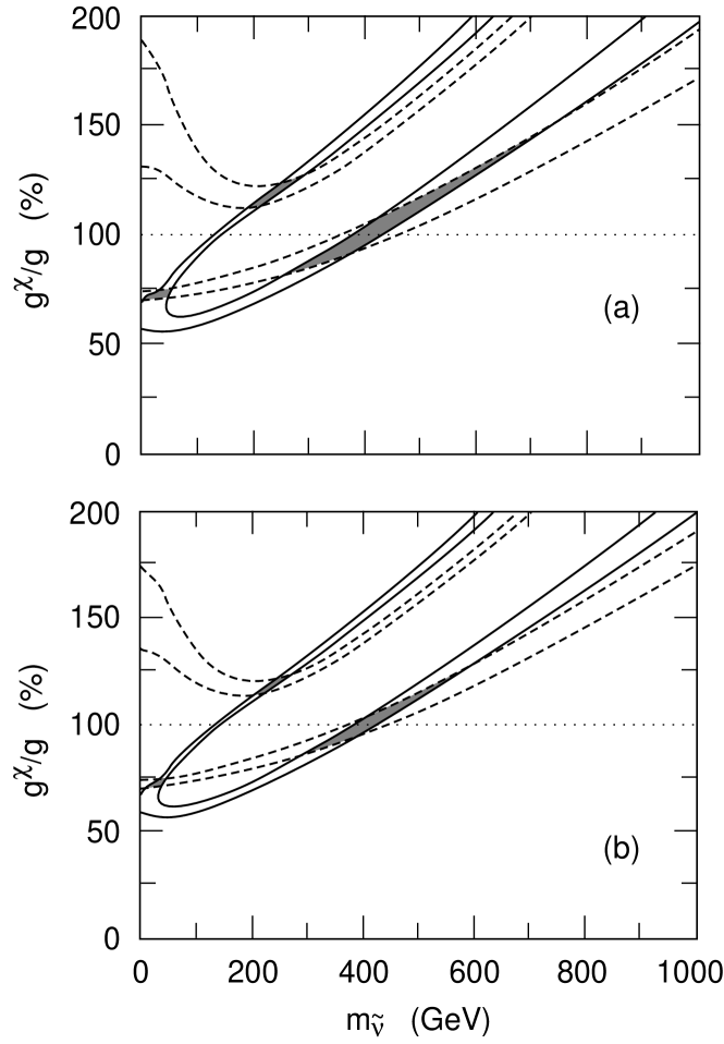
Figure 7: Allowed regions (shaded) of the $(m_{\tilde{\nu}},g^{\chi})$ plane for ${\cal L}_{L}$ = (a) 30 fb^-1 and (b) 100 fb^-1. Solid (dashed) curves are contours of constant $\sigma_{L}$ ($A_{FB}^{\chi}$) that bound the allowed regions. On the dotted lines, the SUSY relation $g^{\chi}=g$ is satisfied.[11]

There is even more excitement after the discovery. Measurement of superparticle masses will tell us physics at very high scales, like GUT- or Planck-scales. The best example is the following test of grand unified theories (GUT) using the masses of gauginos. It is now well-known that the measured value of $\sin^{2}\theta_{W}$ is remarkably consistent with the prediction of supersymmetric GUTs. The reason why we can test a theory at a very high scale in this case is because GUTs predict that the three gauge coupling constants are the same, $\alpha_{1}=\alpha_{2}=\alpha_{3}$ at the GUT-scale. We can extrapolate the measured gauge coupling constants to higher energies, and test whether they meet at a single point. Some people take this seriously, others think it is just a numerical accident. Now supersymmetric GUTs predict further relations. The masses of three gauginos, $M_{1}$, $M_{2}$, $M_{3}$ of bino, wino, and gluino, respectively, also have to be the same at the GUT-scale. Once superparticles are discovered, we can measure their masses, and extrapolate the measured values to higher energies. Then we can see whether they meet at a point. This gives us an independent test of GUTs from that using gauge couping constants, and if verified, it can hardly be an accident.

For such a measurement of gaugino masses, an $e^{+}e^{-}$ linear collider with polarized electron beam is crucial. Since gauginos $\tilde{B}$ and $\tilde{W}$ mix with higgsinos to form two chargino and four neutralino mass eigenstates, one needs to disentangle the mixing to measure the masses of gauginos. In our paper,[10] four experimental observables, $m(\tilde{\chi}_{1}^{0})$, $m(\tilde{\chi}_{1}^{\pm})$, $\sigma(e_{R}^{-}e^{+}\rightarrow\tilde{e}_{R}^{-}\tilde{e}_{R}^{+})$ and $\sigma(e_{R}^{-}e^{+}\rightarrow\tilde{\chi}_{1}^{-}\tilde{\chi}_{1}^{+})$ were used to extract four parameters $M_{1}$, $M_{2}$, $\mu$ and $\tan\beta$. The Fig. 8 shows the accuracy how well one can extract $M_{1}$ and $M_{2}$ consistent with the inputs, which satisfy a simple relation from GUTs. Therefore, one can make an important test of grand unified theories by measuring cross sections and masses of superparticles.

Figure 8: The $\Delta\chi^{2}=1$ contour in the $M_{1}$-$M_{2}$ plane obtained from the global fit.[10] The dotted line indicates the GUT prediction: $M_{1}=(5/3)\tan^{2}\theta_{W}~{}M_{2}$.

Finally, the spectrum of scalar particles will tell us what kind of GUTs it is,[12] or the energy scale where superymmetry is broken (“messenger scale”).[13] Hopefully a combination of the LHC and a linear collider would do this job. There are several differences between supersymmetry studies at the LHC and at a linear collider. The LHC produces superparticles top down. It produces the colored particles like gluino and squarks which are tyipcally 3 to 4 times heavier than their colorless counter parts, and they decay into the lightest superparticle in long chains of cascades. The decay pattern is a complicated function of all low-lying supersymmetry spectrum. Therefore, signature of supersymmetry at the LHC has many important information in it, but it is difficult to sort it out by itself because of very complex cascades. On the other hand, an electron positron linear collider would produce superparticles bottom up. As one raises the center-of-mass energy, the lightest one will be found and subsequently to the heavier ones. At each stage, one studies the newly-found superparticles in detail and determine all the parameters. Then there is no ambiguity in studying the next superparticle because you already know the spectrum below it. This approach is very useful for the colorless superparticles which are supposed to be rather light and likely to be within the reach of a linear collider. The LHC reach of gluino mass up to 2 TeV roughly equals with a 1 TeV linear collider which can find $\tilde{W}$ up to 500 GeV. By determining basic supersymmetry parameters at an $e^{+}e^{-}$ and analyzing the top-down data from the LHC using the inputs from a linear collider, we can eventually sort out the whole superparticle spectrum. This is a challenging, but a very fruitful and exciting program. And having both types of machines is crucial in this grand program.

5 Strong electroweak symmetry breaking sector

Now we come to the discussion of other type of scenario, where the electroweak symmetry is broken by a new strong force. A representative model is technicolor, where this new gauge interaction attracts pairs of technifermions very strongly with each other and let them condense, $\langle\bar{f}f\rangle\neq 0$. The generic signatures of this scenario are: (1) no light Higgs boson (below, say, $600$ GeV), (2) the scattering between two longitudinal $W$ bosons become strong at higher energies (say, $E\mathrel{\mathchoice{\lower 3.0pt\vbox{\halign{$\m@th\displaystyle\hfill#\hfil$\cr>\crcr\sim\crcr}}}{\lower 3.0pt\vbox{\halign{$\m@th\textstyle\hfill#\hfil$\cr>\crcr\sim\crcr}}}{\lower 3.0pt\vbox{\halign{$\m@th\scriptstyle\hfill#\hfil$\cr>\crcr\sim\crcr}}}{\lower 3.0pt\vbox{\halign{$\m@th\scriptscriptstyle\hfill#\hfil$\cr>\crcr\sim\crcr}}}}1.8$ TeV), and (3) there possibly are resonances due to new strong interactions (techni-$\rho$ decaying into $W^{+}W^{-}$ or $W^{\pm}Z^{0}$, techni-$\omega$ into $Z^{0}\gamma$, etc).

First general statement on this scenario is that all experimental signatures are rather rare and weak, and it will be difficult for experiments to see the effects of new strong interaction. Table 3 shows the expected event rates for several different models along with the size of the Standard Model background. Even though it is likely that one can see certain excess in like-sign dilepton with large missing $E_{T}$, it may not be easy to directly interpret it as a signal of strong $WW$ interaction.

Table 3: Expected numbers of events of like-sign dilepton after cuts in the $W^{+}_{L}W^{+}_{L}$ search for an integrated luminosity of $10^{5}$ pb^-1 and for different models, taken from ATLAS TDR.[3] The forward jet tag is used.

Model	Number of events
Standard Model ($m_{h}=1$ TeV)	23
Rescaled $\pi^{+}\pi^{-}$ scattering	25
Low energy theorm (LET)	39
Sharp-cutoff unitarization	40
O(2N) Higgs-Goldstone model	15
Standard Model background	$\mathrel{\mathchoice{\lower 3.0pt\vbox{\halign{$\m@th\displaystyle\hfill#\hfil$\cr<\crcr\sim\crcr}}}{\lower 3.0pt\vbox{\halign{$\m@th\textstyle\hfill#\hfil$\cr<\crcr\sim\crcr}}}{\lower 3.0pt\vbox{\halign{$\m@th\scriptstyle\hfill#\hfil$\cr<\crcr\sim\crcr}}}{\lower 3.0pt\vbox{\halign{$\m@th\scriptscriptstyle\hfill#\hfil$\cr<\crcr\sim\crcr}}}}46$

If one also has an electron positron linear collider in addition to the LHC, this difficult signal becomes convincing. A linear collider can unambiguously prove the absense of any kinds of light Higgs boson below its kinematic reach, $m_{h}\mathrel{\mathchoice{\lower 3.0pt\vbox{\halign{$\m@th\displaystyle\hfill#\hfil$\cr<\crcr\sim\crcr}}}{\lower 3.0pt\vbox{\halign{$\m@th\textstyle\hfill#\hfil$\cr<\crcr\sim\crcr}}}{\lower 3.0pt\vbox{\halign{$\m@th\scriptstyle\hfill#\hfil$\cr<\crcr\sim\crcr}}}{\lower 3.0pt\vbox{\halign{$\m@th\scriptscriptstyle\hfill#\hfil$\cr<\crcr\sim\crcr}}}}0.9(\sqrt{s}-m_{Z})$. The absense of a Higgs boson, combined with an excess in like-sign dilepton, implies a strongly interacting electroweak symmetry breaking sector. Recall that it is not easy to establish the absence of a light Higgs boson at the LHC alone. There is a small hole in the MSSM parameter space which is not easy to cover (Fig. 3). Also, the Higgs boson may decay mainly invisibly, which reduces the $\gamma\gamma$ signature substantially. The invisible decay is not specific to the supersymmetric models, where Higgs bosons may decay into a pair of neutralinos, but also possible in other models as well. For instance if the fourth generation exists with little mixing to lower generations, and if $2m_{\nu_{4}}<m_{H}<2m_{l_{4}}<2m_{q_{4}}$, the Higgs boson decays mainly into $\bar{\nu}_{4}\nu_{4}$ and is hard to be detected. One can also look for associate production processes like $t\bar{t}H$, $WH$ even in this case;[14] but it seems to be not easy to convince ourselves there is no Higgs boson. On the other hand, an invisibly decaying Higgs boson can be easily seen at a linear collider using $Zh$ production with $Z$ decaying leptonically.[6]

So far the role a linear collider plays may seem secondary, just to give a supportive evidence by proving there is no light Higgs boson. But there are more active roles an electron positron linear collider can play as well.

Table 4 shows the significance of strong $WW$ scattering studied at an $e^{\pm}e^{-}$ collider with $\sqrt{s}=1.5$ TeV and an integrated luminosity of 200 fb^-1. The statistical significance is comparable or sometimes better than that at the LHC.

Table 4: Total numbers of $W^{+}W^{-},ZZ\rightarrow 4$-jet signal $S$ and background $B$ events calculated for a 1.5 TeV $e^{\pm}e^{-}$ linear collider with integrated luminosity 200 fb^-1 after cuts. The statistical significance $S/\sqrt{B}$ is also given. The hadronic branching fractions of $WW$ decays and the $W^{\pm}/Z$ identification/misidentification are included. S/N is Improved by using $100\%$ polarized $e^{-}_{L}$ beams in a 1.5 TeV $e^{+}e^{-}/e^{-}e^{-}$ collider.[15]

channels	SM	Scalar	Vector	LET
	$m_{H}=1$ TeV	$M_{S}=1$ TeV	$M_{V}=1$ TeV
$S(e^{+}e^{-}\to\bar{\nu}\nu W^{+}W^{-})$	330	320	92	62
$B$(backgrounds)	280	280	7.1	280
$S/\sqrt{B}$	20	20	35	3.7
$S(e^{+}e^{-}\to\bar{\nu}\nu ZZ)$	240	260	72	90
$B$(backgrounds)	110	110	110	110
$S/\sqrt{B}$	23	25	6.8	8.5
$S(e^{-}e^{-}_{L}\to\nu\nu W^{-}W^{-})$	54	70	72	84
$B$(background)	400	400	400	400
$S/\sqrt{B}$	2.7	3.5	3.6	4.2
$S(e^{-}_{L}e^{-}_{L}\to\nu\nu W^{-}W^{-})$	110	140	140	170
$B$(background)	710	710	710	710
$S/\sqrt{B}$	4.0	5.2	5.4	6.3

If there is a techni-$\rho$ resonance, an electron positron collider will have an ideal signal. The production of $W$-pairs has one of the biggest cross sections at a future $e^{+}e^{-}$ linear collider. If the $W$-bosons in the final state are longitudinally polarized, they can rescatter due to a tail of the techni-$\rho$ resonance. The rescattering modifies various final state distributions of the $W$ decay products. Studies show that one can see the effects of a techni-$\rho$ up to 2 TeV at 95 % confidence level at a linear collider with $\sqrt{s}=500$ GeV and 50 fb^-1,[16] which is already comparable to the reach at the LHC. Fig. 9 contains confidence level contours for the real and imaginary parts ofthe rescattering amplitude $F_{T}$ at $\sqrt{s}=1.5$ TeV with 190 fb^-1.[17] Shown are the 95% confidence level contour about the light Higgs boson value of $F_{T}$, as well as the 68% confidence level contour about the value of $F_{T}$ for a 4 TeV techni-$\rho$. Even the non-resonant LET point is well outside the light Higgs boson 95% confidence level region. The 6 TeV and and 4 TeV techni-$\rho$ points correspond to 4.8$\sigma$ and 6.5$\sigma$ signals, respectively. At a slightly higher integrated luminosity of 225 fb^-1, it is possible to obtain 7.1$\sigma$, 5.3$\sigma$ and 5.0$\sigma$ signals for a 4 TeV techni-rho, a 6 TeV techni-rho, and LET, respectively.

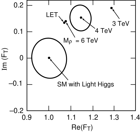
Figure 9: Confidence level contours for the real and imaginary parts of $F_{T}$ at $\sqrt{s}=1.5$ TeV with 190 fb^-1. The initial state electron polarization is 90%. The contour about the light Higgs boson value of $F_{T}=(1,0)$ is 95% confidence level and the contour about the $M_{\rho}=4$ TeV point is 68% confidence level.

The signatures of strong electroweak symmetry breaking sector discussed so far are $WW$ scattering and are relatively model-independent. There are signatures relevant at lower energies, though more model-dependent. Since our aim is to sort out the correct model which describes the electroweak symmetry breaking, such model-dependence is of great interest. Now we turn our discussions to the model-dependent signatures.

First of all, one needs to recall that the scenario of strongly interacting electroweak symmetry breaking sector has many problems. Just to name a few, Peskin–Takeuchi $S$-parameter, flavor-changing neutral currents, typically too small $m_{t}$, large isospin splitting $m_{b}\ll m_{t}$, $R_{b}$, etc. Since it is not so useful to discuss experimental signatures of models which are already excluded, I would like to discuss several attempts to cure some of the above problems. Interestingly enough, such attempts tend to give us signatures at lower energies than a model-independent discusssion gives.

The first example is the $Zt\bar{t}$ vertex. Suppose technicolor theory is right, in the sense that the source of $W$, $Z$ and all fermion masses originate from a single technifermion condensate $\langle\overline{T}T\rangle$. Since $m_{t}$ is large, $\simeq 175$ GeV, there needs to be a fairly strong four-fermi interaction, $\bar{t}t\overline{T}T$. Such an operator can be generated by an exchange of Extended Technicolor (ETC) gauge boson which converts a standard model fermion (top quark in this case) to a techni-fermion. Exchange of such an ETC gauge boson gives an interesting contribution to the $Zb\bar{b}$ vertex.[18] The naive ETC model reduces $R_{b}$, which is the wrong direction given the current tendency in experimental data. There are two modified ETC models which give positive contributions to $R_{b}$, a diagonal ETC boson[19] and a non-commuting ETC gauge boson.[20] In each case, one can choose a parameter such that the additonal contribution is consistent with the current value of $R_{b}$. Interesting point is that these models tend to give a rather large correction to $Zt\bar{t}$ vertex. An analysis[21] shows one can measure vector and axial form factors of the top quark at 10 % level with 50 fb^-1 for each electron beam polarization at $\sqrt{s}=400$ GeV. The predicted values of the vector form factor falls typically outside the 95 % confidence level contour.

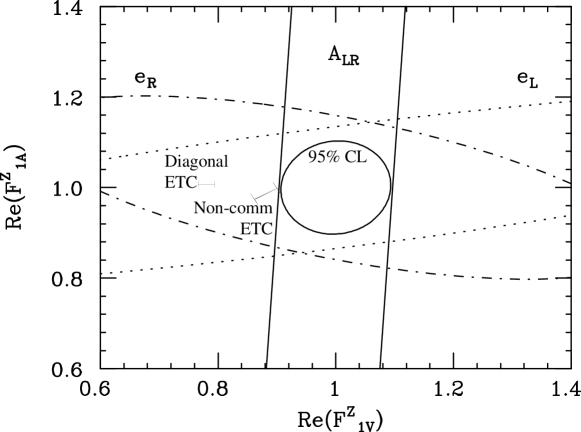
Figure 10: 95% confidence level contours for $F_{1V}^{Z}$ and $F_{1A}^{Z}$, obtained from the maximum-likelihood analysis using a sample of 50 fb^-1 each of right- and left-polarized electrons.[21] Predictions from diagonal ETC[19] and non-commuting ETC[20] put in.[22]

Another interesting model is an attempt to reduce the $S$-parameter which tends to be too large. Since the minimal model of technicolor, one-doublet model with $N_{TC}=2$, is now excluded at more than 99 % confidence level,[23] one needs to find a mechanism to reduce the $S$-parameter. An attempt by Appelquist and Terning[24] is to introduce large isospin splitting, thereby sacrificing $T$-parameter a little, to reduce the $S$-parameter even in a one-family model. Their point is that one can have techni-leptons to be rather light; then the contribution to $T$-parameter can be small enough even when there is a large isospin splitting between techni-electron and techni-neutrino. Their sample spectrum of techni-fermions is

$N$		50	GeV,
$E$		150	GeV,
$Q$		600	GeV.

As apparent from the spectrum, this model predicts light techni-$\rho$, $\overline{N}N$ at 100–300 GeV and a light charged pseudo-Nambu-Goldston boson $N\overline{E}$ at 50–150 GeV. This techni-$\rho$ does not contribute much to the $WW$ rescattering because the techni-neutrino contributes little to the $W$ and $Z$ masses. However it can appear as a narrow resonance in $e^{+}e^{-}$ collision. $N\bar{E}$ can be produced similar to a charged Higgs boson whose main decay mode is $\nu_{\tau}\tau^{+}$. A search for it is straight forward, looking for acoplanar $\tau$-pairs using right-handed electron polarization to suppress the $WW$ background. On the other hand there are many colored psudo-Nambu-Goldstone bosons at 250–500 GeV, which are targets of experiments at the LHC.

There are also attempts to solve the problem of flavor-changing neutral currents which have typically too large rates in extended technicolor models. The mechanism called techni-GIM[25] is one of such attempts. It requires a very complicated gauge strcture and needs many new fermion fields below 1 TeV to cancel anomalies. There typically are many pseudo-Nambu-Goldstone bosons as well, whose masses arise due to gauge interactions. Since colorless pseudo-Nambu-Goldstone bosons are typically lighter than colored one, the situation is quite similar to the supersymmetry. The LHC will look for colored ones, a linear collider for colorless ones.

Summarizing this section, a combination of two observations, (1) the absolute absense of a Higgs boson at a linear collider and (2) a slight excess in $WW$-scattering at the LHC can be a convincing signature of strong electroweak sector. Moreover, the excess in $WW$-scattering observed at the LHC can be cross-checked with a linear collider at $\sqrt{s}=1.5$ TeV; if the excess is due to a techni-$\rho$, $\sqrt{s}=500$ GeV may be already enough. There are other model-dependent signatures like $Zt\bar{t}$ coupling, pseudo-Nambu-Goldstone bosons, light techni-resonances, etc, which help sorting out the correct model. Here again it is clear that the combination of both types of colliders is important to understand physics of electroweak symmetry breaking.

6 Conclusion

Particle Physics is alive and well, it is approaching the most exciting stage of experiments exploring the physics of electroweak symmetry breaking. The combination of the LHC and an electron positron linear collider will allow us to sort out scenarios of electroweak symmetry breaking. Having only one of them may lead to an ambiguous and unsatisfactory exploration of the physics, while having both can give us hints to physics at yet higher energy scales.

References

References

- [1] Yasuhiro Okada, Masahiro Yamaguchi, and Tsutomu Yanagida, Prog. Theor. Phys. 85, 1 (1991); Howard E. Haber and Ralf Hempfling, Phys. Rev. Lett. 66, 1815 (1991); John Ellis, Giovanni Ridolfi, and Fabio Zwirner, Phys. Lett. B 257, 83 (1991).
- [2] JLC-I, JLC Group, KEK-92-16, Dec 1992.
- [3] ATLAS Collaboration, Technical Proposal. CERN/LHCC/94-43 (1994).
- [4] CMS Collaboration, Technical Proposal. CERN/LHCC/94-38 (1994).
- [5] ATLAS Collaboration, “Observability of Minimal Supersymmetric Standard Model Higgs boson at LHC”, Physics Note 074.
- [6] Patrick Janot, Invited talk at 2nd International Workshop on Physics and Experiments with Linear Colliders, Waikoloa, HI, 26-30 Apr 1993.
- [7] M.D. Hildreth, T.L. Barklow, and D.L. Burke (SLAC), Phys. Rev. D 49, 3441 (1994).
- [8] I. Nakamura, talk given at 3rd International Workshop on Physics and Experiments with Linear Colliders, Morioka-Appi, Iwate, Japan, 8–12 Sep 1995.
- [9] J. Gunion and H.E. Haber, private communication; J. Gunion, A. Stange, and S. Willenbrock, to appear in Electroweak Symmetry Breaking and New Physics at the TeV Scale, eds. T. L. Barklow, H. E. Haber, S. Dawson, and J. L. Siegrist, World Scientific, Singapore, 1996.
- [10] Toshifumi Tsukamoto, Keisuke Fujii, Hitoshi Murayama, Masahiro Yamaguchi, and Yasuhiro Okada, Phys. Rev. D D51, 3153 (1995).
- [11] J.L. Feng, M.E. Peskin, H. Murayama, and X. Tata, Phys. Rev. D 52, 1418 (1995).
- [12] Yoshiharu Kawamura, Hitoshi Murayama, and Masahiro Yamaguchi, Phys. Lett. B 324, 52 (1994)/
- [13] M.E. Peskin, plenary talk given at 3rd International Workshop on Physics and Experiments with Linear Colliders, Morioka-Appi, Iwate, Japan, 8–12 Sep 1995.
- [14] J.F. Gunion, Phys. Rev. Lett. 72, 199 (1994); Debajyoti Choudhury and D.P. Roy, Phys. Lett. B 322, 368 (1994); S.G. Frederiksen, N. Johnson, G. Kane, and J. Reid, Phys. Rev. D 50, 4244 (1994).
- [15] V. Barger, Kingman Cheung, T. Han, R.J. Phillips, Phys. Rev. D 52, 3815 (1995).
- [16] A. Miyamoto, K. Hikasa, and T. Izubuchi, KEK Preprint 94-203, “Heavy vector resonance effect on the process at JLC-I.”
- [17] T. Barklow, in the Albuquerque DPF94 Meeting, ed. by Sally Seidel, p. 1236; and references therein.
- [18] R. Sekhar Chivukula, Stephen B. Selipsky, and Elizabeth H. Simmons, Phys. Rev. Lett. 69, 575 (1992).
- [19] Kaoru Hagiwara and Noriaki Kitazawa, Phys. Rev. D 52, 5374 (1995).
- [20] R.S. Chivukula, E.H. Simmons, and J. Terning, Phys. Lett. B 331, 383 (1994).
- [21] T.L. Barklow and C.R. Schmidt, in DPF ’94: The Albuquerque Meeting, ed. by S. Seidel, World Scientific, Singapore, 1995.
- [22] Uma Mahanta, H. Murayama, M.V. Ramana, in preparation.
- [23] Kaoru Hagiwara, Talk given at International Symposium on Lepton Photon Interactions (IHEP), Beijing, P.R. China, 10-15 Aug 1995, hep-ph/9512425.
- [24] T. Appelquist and J. Terning, Phys. Lett. B 315, 139 (1993).
- [25] L. Randall, Nucl. Phys. B 403, 122 (1993); H. Georgi, Nucl. Phys. B 416, 699 (1994).