Critical Behaviour and Universality in Gravitational Collapse of a Charged Scalar Field
Abstract
We summarize results from a study of spherically symmetric collapse of a charged (complex) massless scalar-field [1]. We present an analytic argument which conjecture the generalization of the mass-scaling relation and echoing phenomena, originally discovered by Choptuik, for the charged case. Furthermore, we study the behaviour of the self-similar critical solution under external perturbations – addition of a cosmological constant and a charge-conjugation . Finally, we study the scaling-relation of the black-hole charge. Using an analytic argument we conjecture that black-holes of infinitesimal mass are neutral or obey the relation . We verify our predictions with numerical results.
I INTRODUCTION
Gravitational collapse is one of the most interesting phenomena in general relativity. The dynamics of a spherically-symmetric massless scalar-field coupled to general relativity has two kinds of possible end states. Either the scalar field eventually dissipates away leaving spacetime flat or a black-hole forms. Numerical simulations of this model problem [2] have revealed a very interesting phenomena – a kind of critical behaviour which is a feature of supercritical initial conditions very close to the critical case ( is a parameter which characterizes the strength of the initial configuration, and is the threshold value). More precisely, Choptuik found a power-law dependence of the black-hole mass on critical separation of the form:
| (1) |
Subsequently the same type of critical behaviour has been observed for other collapsing fields: the collapse of axisymmetric gravitational wave packets [3], the collapse of spherically symmetric radiative fluids [4]. In all these model problems the critical exponent turned out to be close to the value originally found by Choptuik , suggesting a universal behaviour. However, Maison [5] has shown that for fluid collapse models with an equation of state given by the critical exponent strongly depends on the parameter .
The second key feature of Choptuik’s results is the universality of the precisely critical evolution at the threshold of black-hole formation – it was found that the critical solution has a discrete self-similar behaviour (discrete echoing with a period ).
In this paper we summarize results from a study of spherically symmetric collapse of a charged (complex) massless scalar field. The main question we consider is whether it is possible to generalize Choptuik’s results for the general charged case [1]. This generalization is not trivial since the introduction of charge-conjugation destroys the invariance of the evolution equations under the rescaling , where is an arbitrary positive constant. This invariance characterizes the system in the special neutral case and is crucial for the self-similarity of the critical evolution. This lack of invariance hints that charge-conjugation might destroy the phenomena in the general situation.
Using a semi-quantitative arguments, which is based upon different behaviour of the mass and charge under the rescaling , we conjecture that the significance and influence of the charge decreases during the evolution and that the critical behaviour appears. Following this we provide a numerical evidence which confirms the generalization of the mass-scaling relation and echoing phenomena for the charged situation.
So far, the mass-scaling relation of the black-hole, and the influence of perturbations on the critical evolution itself, have been studied in context of internal perturbations in the initial conditions, such as a deviation of the field’s amplitude from the critical one. It is of interest to study the behaviour of the critical solution under external perturbations. We consider here the influence of the charge as such a perturbation. We also consider the effect of another external parameter, the cosmological constant .
The plan of the paper is as follows. In Sec. II we describe the evolution equations. In Sec. III we describe the algorithm and numerical methods. In Sec. IV we describe our discretization and error analysis. In Sec. V we describe our theoretical predictions and compare them with our numerical results. Sections V.A and V.B establish both qualitatively and quantitatively as well, the generalization of the mass-scaling relation and echoing phenomena for the charged case. In Sec. V.C we study the behaviour of the critical evolution under two such external perturbations: addition of a cosmological-constant to the critical solution and an addition of a charge-conjugation to critical initial-conditions of a complex neutral scalar-field. We also study the possibility of forming black-holes from subcritical initial conditions using external perturbations. In Sec. V.D we study the charge-mass relation for infinitesimal black-holes. We show that for the black-hole charge tends to zero more rapidly than its mass. From this we conclude that black-holes of infinitesimal mass, which can be created from near–critical evolutions, are neutral, or obey the relation . Our numerical results confirm this conjecture. We end in Sec. VI with a brief summary and conclusions.
II THE EVOLUTION EQUATIONS
We consider a spherically symmetric charged scalar field . This is a combination of two real scalar fields , which are combined into a complex one . The electromagnetic field is described by the potential , which is defined up to the addition of a gradient of a scalar function. The electromagnetic field tensor is defined as , i.e. .
The total Lagrangian of the scalar field and electromagnetic field is [6]:
| (2) |
Where is a constant and is the complex conjugate of .
Varying and independently, one obtains [6]:
| (3) |
and its complex conjugate, and:
| (4) |
We express the metric of a spherically symmetric spacetime in the form [7, 8]:
| (5) |
The radial coordinate is a geometric quantity which directly measures proper surface area, and is a retarded time null coordinate. Here is the two-sphere metric.
Because of the spherical symmetry, only the radial electric field is nonvanishing. This choice satisfies Maxwell’s equation:
| (6) |
We introduce the auxiliary field :
| (7) |
Using the radial component of Eq. (4), we express the charge contained within the sphere of radius , at a retarded time , as:
| (8) |
and the potential as:
| (9) |
The energy-momentum tensor of the charged scalar-field is [6]:
| (10) | |||||
| (11) |
The nontrivial Einstein equations are:
| (12) |
| (13) |
Regularity at the origin requires . The boundary condition forces us to integrate the equations outward, and impose the normalization , which corresponds to selecting the time coordinate as the proper time on the central world line.
The solution at a given depends only on the solution at . We integrate Eq. (12) and obtain:
| (14) |
Using Eqs. (12) and (13), we obtain after integration:
| (15) |
In terms of the variable , the wave-equation Eq. (3) takes the form
| (16) |
Using the characteristic method, we convert the scalar-field evolution-equation Eq. (16) into a pair of coupled differential equations:
| (17) |
| (18) |
We solve these equations together with the integral equations (7), (14), (15), (8) and (9). The mass contained within the sphere of radius at a retarded time , is:
| (19) |
Using Eqs. (14) and (15), we express as:
| (20) |
III ALGORITHM AND NUMERICAL METHODS.
A numerical simulation of the special uncharged case was first performed by Goldwirth and Piran [8]. Gundlach, Price and Pullin [9] used a version of this algorithm to study the scaling behavior of the mass of the black-hole for the special uncharged case. We have used a version of the algorithm of Refs. [8, 10], for the neutral case, and we have generalized it for the charged case. However, the methods used in Refs [8, 9] are not accurate enough for a treatment of the critical solution itself, because each successive echo appears on spatial and temporal scales a factor finer than its predecessor.
The main improvements of our version closely resembles that of Ref. [10]: Taylor expansion of the physical quantities near the origin, conservation of the number of grid points using interpolation and choosing the outermost grid point to be the ingoing light ray that hits the zero mass singularity of the critical solution .
To solve numerically Eqs. (17) and (18) we define a radial grid , where . We should emphasize that is a complex field: , and obtain a set of coupled differential equations.
| (21) | |||||
| (22) |
| (23) | |||||
| (24) |
| (25) |
where and satisfy the boundary conditions
| (26) |
The initial data for the Einstein-scalar-Maxwell equations is just the value of on the initial data surface, , the value of the parameter , and a numerical choice of the initial position in of each ingoing null lines of the grid. The algorithm proceeds as follows: first we integrate along for a fixed and find in succession the quantities and .
The integration is carried out using a three-point Simpson method for unequally spaced abscissas (Even if the grid is evenly spaced initially, it will not remain so during the evolution [8]). We next use Eqs. (21-25), to evolve and one time step forward. We solve the ordinary differential equations using the fifth-order Runge-Kutta method [11]. This process is iterated as many times as necessary: i.e. until either the field disperses or a charged black-hole forms.
The time step is determined so that in each step the change in is less half the distance between it and the null trajectory , i.e.:
| (27) |
Once a null trajectory arrives at the origin , it bounces and disperses along to infinity. The grid-point is therefore lost when the light ray hits the origin.
If for a given shell at some time then it is possible that
| (28) |
will vanish. We identify the formation of a black hole when there is an value that satisfies
| (29) |
In this case are the horizons of the shell.
As we approach the stage when a black-hole forms becomes infinite. In our algorithm this means that the step size . The numerical approach to the horizon is stopped eventually by an overflow of or underflow of . We can, still, estimate where and when a black-hole horizon appears from the condition .
In [9] this method was used to study the scaling behavior of the mass of the uncharged black-hole. However, this method is not accurate enough for a treatment of the critical solution itself. The main improvements of our version for the charged case closely resembles that of Ref. [10] where this method was used to study the critical solution for the special neutral case. We will now describe shortly the sources of inaccuracy and the methods that we use to overcome them.
The first source of an inaccuracy arises from the fact that the expressions for the quantities and contains an explicit factor of which diverges to the origin. We overcome this by using a Taylor expansion of in :
| (30) |
Then we expand the quantities and in , where the expansion coefficients are all functions of and . Thus, in order to treat the solution near the origin one needs to find only these coefficients. This is done by fitting the first three values of to a second-order polynome: i.e. we solve equation (30) for and to obtain and . We then use these coefficients to evaluate the values of and for the first two values of . The values of these quantities for other values of is then determined using a three-point Simpson method for unequally spaced abscissas.
A second source of inaccuracy arises directly from the behavior of the critical solution itself - as the critical solution evolves each successive echo appears on spatial and temporal scales a factor finer than its predecessor. This problem is solved as follows: The number of grid points decreases during the evolution. Once a null trajectory arrives at the origin it bounces and disperses along to infinity. The grid point is therefore lost when the light ray hits the origin. As the number of points decrease by half we double the number of grid points and we interpolate the new grid points which are half way in between the old ones. We chose the outermost grid point in such a way that this ingoing light ray hits the zero-mass singularity of the critical solution itself. Thus the doubling of the grid gives us just the exact logarithmic scaling needed at the origin.
IV DISCRETIZATION AND ERROR ANALYSIS
Our grid is highly nonuniform in if a horizon forms - as we approach to the horizon the step size decreases rapidly. Furthermore, even if the grid is evenly spaced initially, it will not remain so during the evolution [8]. However, when we consider two grids in which one has twice the number of grid points as the other, the coarser grid spacing will remain twice the size of the finer grid, when we consider points at the same physical location. We will discuss, therefore, our numerical convergence in terms of the initial grid spacing.
We denote the relative size of the initial grid spacing by . From the condition (27) we see that the spacing is proportional to . As we have mentioned, we treat Eqs. (17) and (18) as ordinary differential equations in , and we solve these using a fifth-order Runge-kutta method [11], the error-term is .
The calculation of the quantities and in these equations is nontrivial, and is given by Eqs. (7), (8), (14), (15), (9) and (20) respectively. The integrals are discretized using three-point Simpson method, the error term in the integration is , where is the fourth derivative of the integrand [11].
As we go from one grid to a finer one (i.e. doubling the grid when the number of grid points reach half of the original number) we have to interpolate to obtain the values at the new grid points. The error term in the interpolation is .
As was mentioned in [12], the main source of error is the boundary conditions and at . We treat these boundary-conditions by approximating the true value of using an interpolation according to Eq. (30), the error term is . The situation is even more complicated: The right hand-side of (17) contains an explicit factor of , which in the exact solution is canceled by the boundary conditions.
Three reasons lead to the crucial importance of checking the behaviour of the solution near the origin, in order to establish our confidence in the numerical results:
-
1.
The risk of numerical instability caused by the explicit factor of .
-
2.
The solution at some value of depends only on the solution at , so a numerical error in the quantity near , would cause an error at each , and in all the relevant physical quantities.
-
3.
The critical solution itself, which is the main issue of this work, appears on ever smaller spatial scales during its evolution, leading to the formation of a zero-mass singularity at , and the importance of our confidence in the numerical solution near the origin is therefore clear.
As we can see, is the basic quantity which influence all the other physical quantities, and at each and every value of .
Figure 1 displays the error in . In this figure the initial data is of family , with amplitude , and (see V) for a discussion of initial data). For these initial conditions the gravitational field is strong , and the scalar-field undergo a terminal gravitational collapse into a charged black-hole.

Due to the fact that there are no useful analytical solutions available, we use of the numerical solution itself as the reference solution. The reference solution was taken as the solution with 1600 grid-points, and it was compared with the solutions of 800, 400, 200, 100 and 50 grid-points.
The difference of between a given calculation and the reference calculation was squared, summed (for different vales of ) and the square root was taken. The top part of Fig. 1 establishes visually that the code converges: this graph displays the real part of the scalar field for different relative spacing of the grid-points: 1/1600, 1/800, 1/400, 1/200, 1/100 and 1/50. The numerical errors are so small that the six lines (for the different grids) actually overlap.
The bottom part of Fig. 1 establishes empirically the stability and convergence of the code when we decrease the grid spacing: the numerical error varies as , where . The fact that the power is close to 3 at the origin is an indication that this error is caused by our handling of the boundary conditions.
Furthermore, we have performed by a similar manner a calculation of the error in . The top part of Fig. 2 displays again the fact that the numerical errors are so small that the different lines (for the different grids) actually overlap. The bottom part of Fig. 2 establishes once again the stability and convergence of the code: the error varies as , where . This value of the power indicates that in this regime the discretization error due to the interpolation which we use in order to maintain the number of grid-points is dominant.

V THEORETICAL PREDICTIONS VS. NUMERICAL RESULTS
In this section we present our theoretical predictions and numerical results for the gravitational collapse of a scalar field, for both the uncharged and for the charged cases. The numerical results that we present arise from a study of several families of solutions, whose initial scalar field profiles are listed in Table I:
| Family | Form of initial data | |
|---|---|---|
| (a) | 0 | |
| (b) | 0 | |
| (c) | 1 | |
| (d) | 1 |
Families (a) and (b) represent uncharged scalar-field while families (c) and (d) represent charged (complex) scalar-field. The amplitude is the critical parameter .
A THE CRITICAL SOLUTION
In this section we discuss the critical solution itself, both for the previously studied uncharged case and for the newly studied charged one. First, we had to find the value of the critical parameter. This was done by a binary search until we found the value of the critical parameter to the desired accuracy.
Let denote the value of at which the singularity forms. We define
| (31) |
| (32) |
In terms of these variables, the critical solution for the neutral case is characterized by discrete self-similarity [2], i.e. and other form-invariant quantity such as or are periodic functions of .
The generalization to the charged case is not trivial. Charge-conjugation destroys the invariance of the evolution-equations under the rescaling , where is an arbitrary positive constant. This invariance characterizes the system in the neutral case and it is essential for the appearance of critical, self similar behaviour. The lack of this invariance raises the interesting question whether critical behaviour will appear in the charged case.
Using a semi-qualitative argument, which is based upon different behaviour of the mass and charge under the rescaling , we might be able to answer this question. As the critical solution evolves its structure appears on ever smaller spatial (and temporal) scales. For the special neutral case we know that each successive echo appears on spatial and temporal scales which are a factor smaller than its predecessor. Under the rescaling we have:
| (33) | |||||
| (34) | |||||
| (35) | |||||
| (36) | |||||
| (37) | |||||
| (38) |
where are the parts of and which do not depend on , and are the additions in the charged case. Since we learn from Eqs. (33-38) that as the field evolves, the significance and influence of the charge on the evolution near the origin is reduced.
Furthermore, as the oscilations proceed the scalar field approaches a real function times a constant phase [13]. This leads to an addtional decrease in the charge of the form:
| (39) | |||||
| (40) | |||||
| (41) | |||||
| (42) |
where is a positive constant (see Section V.D).
When both effects are combined together decreases with each echo, approximately from . Looking at the right hand side of equation (17) we find that the various terms scale according to
| (43) | |||||
| (44) | |||||
| (45) | |||||
| (46) |
From here we learn that as the evolution proceeds the last three terms in the right hand side of equation (17) becomes smaller relative to the first term by a factor larger than with each echo. From these arguments we expect to find that for near-critical evolutions the influence of the charge on the evolution should decrease with each echo.
We conjecture that in the precisely critical case and in the limit of an infinite train of echoes, the influence of the charge on the evolution near origin is “washed out” and we expect to have the Choptuik solution. In practice, using the fact that we expect the influence of the charge on the evolution to be negligible even after a small number of echoes. Thus, once echoing begins the solution will approach the neutral one rapidly. Our numerical solution verifies these predictions. Fig. 3 shows the quantity max as a function of for near-critical evolution of families (a), (b), (c) and (d). The solutions of families (b)-(d) were shifted horizontally but not vertically with respect to family (a) in order that the first echo of each family will overlap the first echo of family (a). After an initial phase of evolution the quantity max settles down to a periodic behaviour in . The period is which corresponds to previous numerical results found by Choptuik [2] for the neutral case.

Fig. 3 also provides a numerical evidence for the universality of the strong-field evolution of a critical configuration. In order to verify whether or not this universality exist for each and every value we display in Fig. 4 profiles of as a function of for values at which the quantity max takes its maximum as a function of . (It should be emphasized that Fig. 4 is composed of 16 profiles - 4 for each family.) The close similarity of the profiles illustrates two important properties:
-
1.
For each family by itself, the critical solution is periodic. Each successive echo appears on spatial and temporal scales a factor finer than its predecessor.
-
2.
The close similarity of the profiles illustrates the uniqueness of the critical solution, independent of the initial profile and charge.

FIG. 4.: The profiles of for each of the four families, are plotted as a function of the logarithmic coordinate in those times at which the quantity Max reaches its maximum as a function of . (It should be emphasized that this figure is composed from 16 profiles – 4 for each family.) For each family by itself, each echo appears on spatial and temporal scales a factor finer than its predecessor. Furthermore, the close similarity of the profiles illustrates the uniqueness of the critical solution, independent of the critical profile and charge.
B SCALING BEHAVIOR OF THE BLACK-HOLE MASS.
We turn now to the power-law dependence of the black-hole mass. The critical solution by itself does not yield the black-hole scaling relation; we should perturb the critical initial conditions, which has a self-similar character. This would lead to dynamical instability - a growing deviation from the critical evolution towards either subcritical dissipation or supercritical charged black-hole formation. To describe the run-away from the critical evolution we consider a perturbation mode with a power-law dependence [4, 5], where . Assume the range of validity of the perturbation theory is restricted to some maximal deviation from the critical evolution, i.e. the evolution is approximately self-similar until the deviation from the critical solution reach the value . From here on the evolution is outside the scope of the perturbation theory – there is subcritical dissipation of the field or supercritical black-hole formation. In either case, the evolution from this stage on has no self-similar character.
We assume the perturbation in the initial conditions develops into a charged black-hole the time requires in order to have a deviation from the critical solution is given by the relation
| (47) |
Of course, a bigger initial perturbation requires a smaller time – the horizon is formed sooner. The logarithmic time is given by
| (48) |
where depends on and .
In a following paper [1, 14] we prove that in order to have the total logarithmic time until the horizon formation one should add a periodic term with a universal period, , which depends on the previous universal parameters according to: , so that the full dependence of on critical separation , for the neutral case as well as for the charged case, is given by
| (49) |
Fig. 5 displays as a function of , where , for the neutral families (a), (b) and for the charged families (c), (d) as well. The points are well fit by a straight line whose slope is . This is consistent with the relation (49).

The exponent is related to the critical exponent that describes the power-law dependence of the black-hole mass. We define as the mass after echoes. Following this definition we define
| (50) |
where is the part of which does not depend on and is the charge contribution in the charged case. From (38 and 42) it follows that
| (51) |
We substitute (48) into (51) and obtain
| (52) |
and find that and is a family-dependent constant. Here we have assumed that and do not depend on .
Thus, according to the perturbation theory, the critical exponent describes both the system’s response to perturbations to the critical evolution, and the deviation rate from it. In a following paper [14, 1] ***see also [15] we show that one should add a periodic term with a universal period to the scaling relation (52).
Fig. 6 displays as a function of for the neutral families (a), (b) and for the charged families (c) and (d) as well, where is the normalized black-hole mass in units of the initial mass in the critical solution. The points are well fit by a straight line whose slope is . This is consistent with the prediction according to which . The measured value of the critical parameter in the charged case agrees with the one of Choptuik for the special non-charged case. Thus, Fig. 6 presents a generalization of the mass-scaling phenomenon for the charged case.

In the neutral case the black-hole mass is proportional to its radius and either the mass or the radius could be the physical order-parameter. In the charged case the black hole radius equals and in general it is no longer proportional to . However, as we approach the critical-solution, the significance of the charge decreases with each echo. The quantity becomes smaller as the black-hole mass gets smaller and it is impossible to distinguish between the two possibilities.
C EXTERNAL PERTURBATIONS TO THE CRITICAL SOLUTION
So far, the mass-scaling relation of the black-hole, and the influence of perturbations on the critical evolution itself, have been studied in context of internal perturbations in the initial conditions, such as a deviation of the field’s amplitude from the critical one. It is of interest to study the behaviour of the critical solution under external perturbations. In particular, we have studied the behaviour of the critical evolution under two external perturbations:
-
1.
Addition of a cosmological-constant to the critical solution itself.
-
2.
An addition of a charge-conjugation to critical initial-conditions of a complex neutral scalar-field.
Adding an external perturbation to the critical solution, which has a self-similar character, is expected to yield dynamical instability – a growing deviation from the critical evolution toward either subcritical dissipation or supercritical black-hole formation. In the situation where the external perturbation to the critical solution (which, in the unperturbed case, is expected to form a zero-mass singularity) leads to a formation of a black-hole, we have studied the question whether or not there is a power-law dependence of the black-hole mass on the external parameter: or .
1 Addition of a cosmological constant
The amplitude was first set to its critical value (for ). We then add a cosmological-constant, , and study its influence on the evolution of the critical solution. led to a dissipation of the critical solution and, on the other hand, was found to give a finite-mass black-hole formation.
We have studied the behaviour of the black-hole mass as a function of the cosmological constant. This is analogue to the addition of an external magnetic field to a system of magnetic moments and studying the magnetization dependence on the strength of the external field exactly at the critical temperature (at the magnetization is zero without an external magnetic field, just as the zero-mass singularity for and ). The analogy arises from the fact that in both cases the external perturbation, magnetic-field or a cosmological-constant, forces the order-parameter to have a non-zero value at or at , correspondingly.
For , the generalization of Eq. (15) is
| (53) |
In addition, one should add the term
| (54) |
in the right-hand side of Eq. (17). Evidence for the universality and the power-law dependence of the black hole mass on the external parameter is shown in Fig. 7 which displays as a function of for critical initial-conditions . The points are well fit by a straight line, i.e.
| (55) |
where .

2 Addition of a charge-conjugation
The amplitude was first set to its critical value for the families (c) and (d), with . For , the initial conditions represent uncharged complex scalar-field. We then add a charge-conjugation, , and studied its influence on the evolution of the critical solution. We have studied the behaviour of the black-hole mass as a function of the charge-conjugation (keeping the amplitude on its critical value ). The numerical results are shown in Fig. 8, which displays as a function of . The points are well fit by a straight line, i.e.
| (56) |
where .

In order to have a more detailed picture of the formation for a charged black-hole near the phase-transition we have studied the conditions required the formation of a charged black-hole and the dependence of its mass on the critical separation and on the charge-conjugation . This was done both for subcritical initial-conditions and for supercritical initial conditions as well, which are close to the phase-transition .
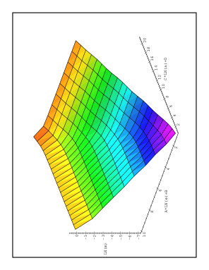
Fig. 9 displays the dependence of the black-hole mass which forms from subcritical initial conditions as a function of and , for family (c). This provides a numerical evidence for the conjecture that external perturbation such as charge-conjugation can lead to a black-hole formation with subcritical initial-conditions . Charge oppose gravitation but the electromagnetic energy density also contributes to the gravitational binding, and by doing so it permits the formation of a black-hole even from subcritical initial-conditions.
The critical charge-conjugation , needed to obtain large enough deviations from the otherwise evolution, followed by black-hole formation from subcritical initial conditions, is well described by a power-law dependence on critical-separation :
| (57) |
where (see Fig. 10).

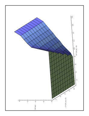
Fig. 11 displays the dependence of the black-hole mass formed from supercritical initial conditions as a function of and , for family (c). We learn that near the phase-transition, the larger the critical separation and the charge-conjugation , the larger is the black-hole mass. The slope of the right edge of the surface is , which is consistent with Eq. (52). The slope of the left edge of the surface is , which is consistent with Eq. (56).
It should be emphasized that the tight relation between the various critical-exponents and , which all describe the instability of the critical evolution under a variety of different perturbations, is a strong evidence supporting the conjecture that there exists one mechanism which can explain the power-law dependence of the black-hole mass on the various parameters, both for internal perturbations in the initial conditions, and for external perturbations as well.
D THE CHARGE-MASS RELATION FOR BLACK HOLES
We have shown in 5.A that the black-hole charge tends to zero faster than its mass for . We demonstrate now that as a power law with a critical exponent larger than (see also [13] for an independent analysis of this problem).. Define as the charge after echoes. From (35 and 39) it follows that
| (58) |
Substituting (48) into (58) and assuming that does not depend on we obtain
| (59) |
where is a family-dependent constant.
From this analytic argument we deduce two conclusions:
-
1.
The black-hole charge is expected to have a power-law dependence on critical separation , where the critical-exponent is closely related to the critical-exponent of the mass according to .
-
2.
The black-hole charge tends to zero with more rapidly than its mass.
Fig. 12 displays as a function of for near-critical black-holes, where is the normalized black-hole charge in units of the initial-charge in the critical-solution. The points are well fit by a straight line whose slope is . This is consistent with the relation (59).

Another way to determine the value of is directly from Eqs. (58 and 59). Fig. 13 displays as a function of , the number of echoes, along the critical solution. The slope is . Using and we find , in agreement with the prediction, , of Gundlach and Martin-Garcia[13] .

The data shown in Figs. 12 and 13 come from the charged family (c). For family (d) we have found that in general the charge increases as the critical separation increases although this correlation is not well described by a power-law dependence. The reason for this situation probably comes from the initial stage of the evolution (note that the initial data contains layers of both positive and negative charge whose relative magnitude depends on . Consequently, the assumption that does not depend on breaks down for this configuration.
Despite of this, our numerical results qualitatively confirm our prediction – the black-hole charge tends to zero with faster than its mass. From here we conclude black-holes with infinitesimal mass, which, according to this mechanism, can be created from near-critical evolutions, are neutral, or obey the relation .
VI SUMMARY AND CONCLUSION
We have studied the spherical gravitational collapse of a charged (complex) scalar-field. The main issue considered is the generalization of the critical behaviour, originally discovered by Choptuik for neutral fields, for the general charged case. This generalization is not trivial, since the introduction of a charge-conjugation destroys the invariance of the evolution equations under the rescaling , which characterizes the system in the neutral case and is crucial for the self-similarity of the critical evolution. This lack of invariance hints that charge-conjugation might destroy the phenomena in the general situation.
However, we have shown that the significance and influence of the charge decreases during the evolution and consequently the critical behaviour appears. As the black-hole charge tends to zero faster than its mass, i.e. . Thus, we conjecture that black-holes of infinitesimal mass, which can be created from near-critical evolutions, are neutral, or obey the relation . Consequently, we find both the mass scaling relations for supercritical solutions and the echoing phenomenon for the critical solution. The charge of the black hole also depends, as a power law on the separation from criticality. The critical exponent, is .
We have also studied the response of the critical solution to external perturbations. In particular, we have studied the behaviour of the critical evolution under an addition of a cosmological-constant , and an addition of charge-conjugation to critical initial-conditions of a complex neutral scalar-field. We have found a power-law dependence of the black-hole mass on external parameters and .
Under the influence of these external perturbations it is possible to form black-holes from subcritical initial conditions. Once more, the critical charge-conjugation , which is needed to form black-holes from subcritical initial-conditions, is well described by a power-law dependence on critical separation .
Acknowledgements.
We thank Amos Ori for helpful discussions and Carsten Gundlach for critical remarks. This research was supported by a grant from the US-Israel BSF and a grant from the Israeli Ministry of Science.REFERENCES
- [1] S. Hod, MSc. thesis, The Hebrew University, Jerusalem, (1995).
- [2] M.W. Choptuik, Phys. Rev. Lett. 70, 9-12 (1993).
- [3] A.M. Abrahams and C.R. Evans, Phys. Rev. Lett. 70, 2980-2983 (1993).
- [4] G.R. Evans and J.S. Coleman, Phys. Rev. Lett. 72, 1782-1785 (1994).
- [5] D. Maison, Phys. Lett. B366, 82 (1996).
- [6] S.W. Hawking and G.F.R. Ellis, The Large Scale Structure of Space Time, Cambridge University Press, (1973).
- [7] D. Christodoulou, Commun. Math. Phys. 105, 337-361 (1986).
- [8] D.S. Goldwirth and T. Piran, Phys. Rev. D36, 3575-3581 (1987).
- [9] C. Gundlach, R.H. Price and J. Pullin, Phys. Rev. D49 890-899 (1994).
- [10] D. Garfinkle, Phys. Rev. D51, 5558-5561 (1995).
- [11] W.H. Press, S.A. Teukolsky, W.T. Vetterling and B.P. Flannery, Numerical Recipes in Fortran: The Art of Scientific Computing, 2nd ed., Cambridge University Press, Cambridge, 1992.
- [12] M.W. Choptuik, D.S. Goldwirth and T. Piran, Class. Quantum Grav. 9, 721-750 (1992).
- [13] C. Gundlach, J. M. Martin-Garcia, gr-qc 9606072 (1996).
- [14] S. Hod and T. Piran, preprint, gr-gc 9606087 (1996).
- [15] C. Gundlach, gr-qc 9604019 (1996).