Fermilab Conf-95/288

Sept. 1995

$B_{s}$ Mixing via $\psi K^{*}$

Patricia McBride 

Fermilab, Batavia, IL 60510

Sheldon Stone 

Physics Dept., Syracuse Univ., Syracuse N.Y. 13244

Abstract

The decay mode $B_{s}\to\psi\overline{K}^{*}$ is suggested as a very good way to measure the $B_{s}$ mixing parameter $x_{s}$. These decays can be gathered using a $\psi\to\ell^{+}\ell^{-}$ trigger. This final state has a well resolved four track decay vertex, useful for good time resolution and background rejection.

Presented at

BEAUTY ’95 - 3rd International Workshop on B-Physics at Hadron Machines

1 Introduction

Measurement of $B_{s}$ mixing would accurately determine one side of the so called “unitarity” triangle, because theoretical uncertainties mostly cancel when the ratio of $B_{s}$ to $B_{d}$ mixing is used [1].

Time dependent mixing measurements using dileptons at LEP have given precise values for the mixing parameter $x_{d}$, and have shown that $x_{s}>8$ at 90% confidence level [2]. Standard model expectations are that $60>x_{s}>12$ [3]. In order to make these measurements the decay time is calculated according to:

$$t={L\over{c\beta\gamma}},$$ (1)

where $L$ is the decay length, c the speed of light and $\beta\gamma$ is equal to the momemtum divided by the mass. The error in $t$ is given by

$$\sigma^{2}_{t}=\left(\sigma_{L}\over c\beta\gamma\right)^{2}+\left(t\sigma_{\beta\gamma}\over\beta\gamma\right)^{2},$$ (2)

where the first term arises from the error in decay length and the second arises from the error in determining the $B_{s}$ momentum.

Use of several modes have been suggested for measuring $x_{s}$ with a $D_{s}^{+}$ in the final state. They are listed in Table 1 along with their predicted branching ratios [4].

Table 1: Branching Ratios for $B_{s}\to D_{s}$ Decays

Mode	$B_{s}$ rate	Product branching fraction
$D_{s}^{+}\ell^{-}\overline{\nu}$	0.105	$9\times 10^{-3}$
$D_{s}^{+}\pi^{-}$	$(2.6\pm 0.4)\times 10^{-3}$	$1.1\times 10^{-4}$
$D_{s}^{+}\pi^{+}\pi^{-}\pi^{-}$	$(6.3\pm 2.6)\times 10^{-3}$	$2.7\times 10^{-4}$
The observable rate for $D_{s}^{+}\to K^{+}K^{-}\pi^{-}$ through the
intermeadiate states $\phi\pi^{+}$ and $K^{*o}K^{-}$ is taken as 4.3%.

Unfortunately, there are several problems with using these modes to measure $x_{s}$. The semileptonic decay has a large branching ratio, 21% for the sum of $\mu$ and electron modes, but the undetected neutrino causes the determination of the $B_{s}$ momentum to have a relatively large uncertainty. This limits the maximum possible $x_{s}$ reach to about 12.

The $D_{s}^{+}\pi^{-}$ mode has a relatively low branching ratio. Furthermore, the $B$ decay vertex must be constructed by first forming a $D_{s}$ decay vertex and then swimming back this vector to intersect with the $\pi^{-}$. There also may be combinatorial background problems as $D_{s}$ production in $B$ decays is substantial, about 12%. The background problems could be worse in the higher multiplicity $D_{s}^{+}\pi^{+}\pi^{-}\pi^{-}$ mode.

2 Use of $B_{s}\to\psi\overline{K}^{*}$, $\overline{K}^{*}\to K^{\mp}\pi^{\pm}$

The simplest $B_{s}$ final states with $\psi$ mesons are $\psi\eta$ and $\psi\phi$. Neither of these can be used to measure $B_{s}$ mixing because they are not flavor specific, i.e. the final state can arise either from a $B_{s}$ or a $\overline{B_{s}}$. Several years ago the Cabibbo suppressed decay $B_{s}\to\psi\overline{K}^{*}$, $\overline{K}^{*}\to K^{\mp}\pi^{\pm}$ was suggested as a possible way to investigate mixing phenomena [5]. Here the sign of the kaon charge distinguishes between $B_{s}$ or $\overline{B}_{s}$.This mode would proceed via the diagram shown in Fig. 1. The recent CLEO observation of $B^{-}\to\psi\pi^{-}$ decays at the level expected from Cabibbo suppression is good evidence for the existance of such diagrams [6]. They measure

$${{\cal B}(B^{-}\to\psi\pi^{-})\over{\cal B}(B^{-}\to\psi K^{-})}=(5.2\pm 2.6)\%\approx\lambda^{2}.$$ (3)

We predict the branching ratio

$${\cal B}(B_{s}\to\psi\overline{K}^{*})={\cal B}(B_{d}\to\psi K^{*})\times\lambda^{2}=1.7\times 10^{-3}\times 0.05=8.5\times 10^{-5}.$$ (4)

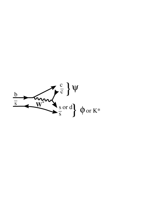
Figure 1: Weak decay diagrams for $\overline{B}_{s}\to\psi\phi$ and $\psi K^{*}$. The $K^{*}$ final state occurs when the virtual $W^{-}$ materializes as a $\bar{c}d$ pair.

Another way of describing the yield of these decays is to form the ratio with respect to $\psi K_{s}$. We have

$${{\cal N}(B_{d}\to\psi K_{s})\over{\cal N}(B_{s}\to\psi\overline{K}^{*})}={{\cal B}(B_{d}\to\psi K_{s})\times{\cal B}(K_{s}\to\pi^{+}\pi^{-})\times{\cal B}(\psi\to\mu^{+}\mu^{-})\over{\cal B}(B_{s}\to\psi\overline{K}^{*})\times{\cal B}(\overline{K}^{*}\to K^{-}\pi^{+})\times{\cal B}(\psi\to\mu^{+}\mu^{-})}=5,$$ (5)

where ${\cal N}$ indicates the number of observed events, for an equal sample of $B_{d}$ and $B_{s}$. We have assumed that the detection efficiency for $\overline{K}^{*}\to K^{-}\pi^{+}$ is equal to that for $K_{s}\to\pi^{+}\pi^{-}$. We expect, however, that the $K_{s}$ efficiency is significantly lower due to the long decay distance of the $K_{s}$. We need to correct for the difference in the relative production ratio between $B_{d}$ and $B_{s}$. An estimate is obtained from LEP data by using the measurement of the ratio of opposite sign dileptons to like sign dileptons and comparing with the same number found at the $\Upsilon(4S)$, where $B_{s}$ aren’t produced. Such a calculation gives 1/3-1/4 the number of $B_{s}$ relative to the number of $B_{d}$. Therefore we expect about 1/15 the number of reconstructed and flavor tagged $B_{s}\to\psi\overline{K}^{*}$ as $B_{d}\to\psi K_{s}$. For hadron collider experiments several thousand tagged $\psi K_{s}$ events implies several hundred tagged $\psi\overline{K}^{*}$ events.

There are several significant advantages using the $\psi\overline{K}^{*}$ decay mode. A $\psi\to\ell^{+}\ell^{-}$ trigger can be used to select these events. Furthermore, this decay mode has a particularly useful topology, having four charged tracks emanating from a single decay vertex. This is important both for background reduction and for exquisite decay time resolution.

Let us consider the $x_{s}$ sensitivity. With this fully reconstructed mode the momentum resolution can be made very good, so there is little effect from the error in $\gamma$ (second term in equation 2). We have made estimates of the time resolution possible in both “forward” and “central” detectors at the FNAL collider. These detectors consist of silicon strips, tracking chambers and have a dipole field for the foward detector and a solenoidal field for the central detector. The simulation program is capable of correctly taking into account the track smearing due to multiple scattering and detector resolution, although the full pattern recognition is not attempted. While detailed resolutions are subject to exact detector configurations some clear conclusions have emerged. We show the time resolution as a function of pseudorapidity ($\eta$) for the forward and central geometries in Fig. 2. Similarly the time resolution is plotted as a function of $\beta\gamma$ in Fig 3.

Figure 2: The time resolution plotted as a function of $\eta$ for a forward detector $(2.0<\eta<4.5)$ and a central detector $(|\eta|<1.5)$ for the decay $B_{s}\to\psi\overline{K}^{*}$ produced at a hadron collider with a center of mass energy of 1.8 TeV.

Figure 3: The time resolution plotted as a function of $\beta\gamma$ for a forward detector $(2.0<\eta<4.5)$ and a central detector $(|\eta|<1.5)$ for the decay $B_{s}\to\psi\overline{K}^{*}$ produced at a hadron collider with a center of mass energy of 1.8 TeV.

The time resolution, $\sigma_{t}$ for the forward geometry is approximately 0.02 ps, while it is about a factor of 10 worse, 0.2 ps for the central geometry. $\sigma_{t}$ appears to be independent of $\eta$ and independent of $\gamma$ for $\gamma>2.$ The latter can be understood as being a result of poorer decay length resolution in direct proportion to $\gamma$, a well know effect explained by the folding in spatial angle of the decay products as $\gamma$ increases. The superiority of the forward geometry results from the decay tracks not being limited from multiple scattering and the ability to place detectors with inherent 10$\mu$m resolution inside the beam pipe.

The number of events as a function of decay time is given by

$$N(t)=N_{o}e^{-{t\over\tau}}\left(1+cos(x_{s}{t\over\tau})\right).$$ (6)

These oscillations are rather rapid on the scale of the $B_{s}$ lifetime, $\tau$. A picture is shown in Fig. 4, where we have also included a Gaussian showing the smearing caused by have a time resolution of 0.05 ps. This resolution was chosen from a naive formula, that the time resolution will cause degradation in the $x_{s}$ measurement if it is poorer than $1/x_{s}$ (in units of ps). Thus, the good time resolution of the forward FNAL type detector in the $\psi K^{*}$ mode would allow a measurement of $x_{s}$ up to values of approximately 50. The average $\gamma$ for accepted decays is 9.5, giving an average decay length of 4.3 mm. For this $\gamma$ the resolution in decay length is 50 $\mu$m.

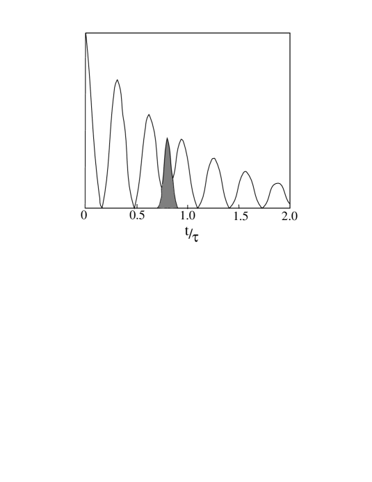
Figure 4: The time distribution $e^{-}{t\over\tau}\{1+cos\left(x_{s}{t\over\tau}\right)\}$ for $B_{s}$ decay for $x_{s}=20$. The shaded region shows a Gaussian with time resolution of 0.05 ps.

To estimate the real reach in $x_{s}$ for a particular experimental proposal requires studies not only of the vertex resolution, but of the backgrounds and fitting procedure as well. It is not the purpose of this paper to present such results. However, the measurement of this channel sets some requirements for a B detector. A detector with good vertex resolution will be able to take advantage of the clean $J/\psi$ signal and the four track $B$ decay vertex to significantly reduce the background from generic $B$ decays. Excellent mass resolution will be needed to eliminate backgrounds from $B^{0}_{d}\to J/\psi K^{*}$. Excellent particle identification will be required to identify the $K$ and $\pi$ in the $K^{*}$ decay and to remove background from other channels such as $B_{s}\to J/\psi\phi$.

Previous attempts at comparing various experiments [7] have used a naive estimate that the number of tagged $B_{s}$ required to measure $x_{s}$ to 20% of its value (i.e. 5 $\sigma$ requires a number of events:

$$N_{req}={5^{2}\over D^{2}d^{2}_{time}},$$ (7)

where $D$ is the dilution from mistagging including away side mixing and $d_{time}$ is the dilution from having finite time resolution. $D$ is taken as approximately 0.5 for most experiments. For $x_{s}<1/\sigma_{t}$, $d_{time}$ is close to one. Therefore it appears that it only takes a few hundred fully reconstructed and tagged $\psi K^{*}$ events to measure $x_{s}$ anywhere within the standard model range. We encourage a full Monte Carlo simulation of this process.

3 Conclusions

The decay mode $B_{s}\to\psi\overline{K}^{*}$ can be used to measure $x_{s}$. It is relatively easy to trigger on the $\psi\to\ell^{+}\ell^{-}$ decay. It has been shown that a forward detector in a hadron collider has excellent time resolution, of the order of 0.02 ps, which is sufficient to measure $x_{s}$ within the standard model range should a few hundred tagged events be accumulated.

References

- [1] H. Schroder, “ Mixing,” in Decays 2nd Editions, ed. S. Stone, World Scientific, Singapore (1994) p449, and references contained therein.
- [2] A. Stocchi, “ and Time Dependent Oscillations,” in these proceedings.
- [3] S. Stone, “Probing the CKM Matrix with Decays,” in The Albuquerque Meeting, ed. S. Seidel, World Scientific, Singapore (1995) p871.
- [4] The branching ratios are assumed to be equal to the branching ratios. In the case of the three pion final state, it is also assumed that rate for is equal to the rate for .
- [5] S. Stone, “ Physics at the SSC,” in Proc. of the 1991 Symposium on the SSC,” Corpus Christi, TX, SSCL-SR-11213 (1991) p225.
- [6] J. Alexander et al., (CLEO) Phys. Lett. B 341, 435 (1995); erratum ibid 347, 469 (1995).
- [7] T.H. Burnett, “Methodology for Comparison of -Mixing Experiments,” in ”Proc. of the Workshop of Physics at Hadron Accelerators,” ed. P. McBride and C.S. Mishra, Fermilab-CONF-93/267 (1993) p367.