Studies of Topological Distributions of Inclusive Three– and Four–Jet Events in Collisions at GeV with the DØ Detector
Abstract
The global topologies of inclusive three– and four–jet events produced in interactions are described. The three– and four–jet events are selected from data recorded by the DØ detector at the Tevatron Collider operating at a center–of–mass energy of GeV. The measured, normalized distributions of various topological variables are compared with parton–level predictions of tree–level QCD calculations. The parton–level QCD calculations are found to be in good agreement with the data. The studies also show that the topological distributions of the different subprocesses involving different numbers of quarks are very similar and reproduce the measured distributions well. The parton shower Monte Carlo generators provide a less satisfactory description of the topologies of the three– and four–jet events.
Abstract
Introduction
The Fermilab Tevatron Collider provides a unique opportunity to study the properties of strong interactions in collisions at short distances. The hard scattering is described by the theory of perturbative Quantum Chromodynamics (QCD) [5, 6, 7] and has been studied extensively in the last decade [8, 9]. Within the context of QCD, the hard process is described as a point–like scattering between constituent partons (quarks and gluons) of protons and anti–protons. The scattering cross sections can be written in expansions in terms of powers of the strong coupling constant convoluted with parton momentum distributions inside the nucleon. The lowest order term corresponds to the production of two–parton final states. Terms of order and in the expansion imply the existence of three– and four–parton final states, respectively. Colored partons from the hard scattering evolve via soft quark and gluon radiation and hadronization processes to form observable colorless hadrons, which appear in the detector as localized energy deposits identified as jets. High energy jets originating from partons in the initial hard scattering process are typically isolated from other collision products. They are expected to preserve the energy and direction of the initial partons, and therefore the topologies of the final jet system are assumed to be directly related to those of the initial parton system.
The cross section and angular distributions for two–jet events have been successfully compared with the predictions of QCD [9, 10]. A study of three– and four–jet events allows a test of the validity of the QCD calculations to higher order ( or beyond) and a probe of the underlying QCD dynamics. This paper explores the topological distributions of three– and four–jet events. The distributions provide sensitive tests of the QCD matrix element calculations. Topological distributions for the three– and four–jet events have been published previously by the UA1, UA2 and CDF Collaborations [11, 12, 13, 14]. However, all of these studies imposed requirements on the topological variables themselves, and therefore significantly reduced the phase space under study. This paper extends these studies to previously untested regions of phase space for a large number of topological variables. The measured normalized distributions, without restrictions on the topological variables themselves, are compared with the QCD tree–level matrix element calculations. The predictions from simple phase–space matrix elements are shown as a comparison, and the distributions of QCD subprocesses involving different numbers of quarks are also examined. Finally, the data are compared with the predictions of three parton shower event generators.
Definition of Topological Variables
The topological variables used in this paper are defined in the parton or jet center–of–mass system (CMS). The definitions refer to partons and jets interchangeably. The partons are assumed to be massless and the jet masses are ignored by using the measured jet energies as the magnitudes of jet momenta.
The topological properties of the three–parton final state in the center–of–mass system can be described in terms of six variables. Three of the variables reflect partition of the CMS energy among the three final–state partons. The other three variables define the spatial orientation of the planes containing the three partons. It is convenient to introduce the notation for the three–parton process. Here, numbers 1 and 2 refer to incoming partons while the numbers 3, 4 and 5 label the outgoing partons, ordered in descending CMS energies, i.e. . The final state parton energy is an obvious choice for the topological variables for the three–parton final state. For simplicity, is often replaced by the scaled variable , which is defined by , where is the center–of–mass energy of the hard scattering process. By definition, . The scaled parton energies and the angles between partons () for the three–parton final state have the following relationship:
| (1) |
where and . Clearly, the internal structure of the three–parton final state is completely determined by any two scaled parton energies. The angles that fix the event orientation can be chosen to be: (1) the cosine***Unless otherwise specified, the absolute values of the cosines of polar angles are implied throughout this paper. of the polar angle with respect to the beam () of parton 3, (2) the azimuthal angle of parton 3 (), and (3) the angle between the plane containing partons 1 and 3 and the plane containing partons 4 and 5 () defined by:
| (2) |
where is the parton momentum. Figure 2 illustrates the definition of the topological variables for the three–parton final state. For unpolarized beams (as at the Tevatron), the distribution is uniform. Therefore, only four independent kinematic variables are needed to describe the topological properties of the three–parton final state. In this paper, they are chosen to be , , and .
Another set of interesting variables is the scaled invariant mass of jet pairs:
| (3) |
where is the invariant mass of partons and and is the opening angle between the two partons. The scaled invariant mass () is sensitive to the scaled energies of the two partons, the angle between the two partons, and the correlations between these variables. Using dimensionless variables and making comparisons of normalized distributions minimizes the systematic errors due to detector resolution and jet energy scale uncertainty and therefore allows a direct comparison between data and theoretical calculation.
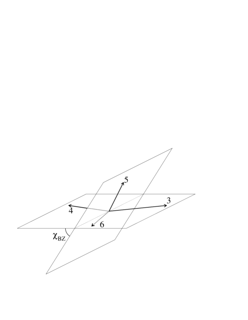
The four–parton final state is more complicated. Apart from the CMS energy, eight independent parameters are needed to completely define a four–parton final state in its center–of–mass system. Two of these define the overall event orientation while the other six fix the internal structure of the four–parton system. In contrast to the three–parton final state, there is no simple relationship between the scaled parton energies and the opening angles between partons. Consequently, the choice of topological variables is less obvious in this case. In this paper, variables are defined in a way similar to those investigated for the three–parton final state. The four partons are ordered in descending CMS energy and labeled from 3 to 6. The variables include the scaled energies (), the cosines of polar angles () of the four jets, the cosines of the opening angles between partons (, and ), and the scaled masses ( and ) of parton pairs. In addition, two variables characterizing the orientation of event planes are investigated. One of the two variables is the “Bengtsson–Zerwas” angle () [15] defined as the angle between the plane containing the two leading jets and the plane containing the two non–leading jets:
| (4) |
The other variable is the cosine of the “Nachtmann–Reiter” angle () [16] defined as the angle between the momentum vector differences of the two leading jets and the two non–leading jets:
| (5) |
Figure 2 illustrates the definitions of and variables. Historically, and were proposed for collisions to study gluon self–coupling. Their interpretation in collisions is more complicated, but the variables can be used as a tool for studying the internal structure of the four–jet events.
The Theoretical Model
The cross section for the production of the –parton final state , in collisions at a center–of–mass energy is described by the following expression:
| (6) |
where the sum runs over all possible parton subprocesses. The functions and are the parton density functions of the incoming partons, represents the matrix elements of the subprocess, and is the –body phase space. Theoretically is well behaved if calculated to all orders in the expansion. At present, this calculation is technically not possible and one has to deal with truncated expansion. As a result, diverges when the energy of any final state parton or the angle between any two partons approaches zero. The singularities in cause poles in the topological distributions. In comparison, a phase–space model in which where does not have singularities in the matrix element, therefore, the topology of the model is determined by the phase space . In this paper, the distributions from the phase–space model are used as references for the comparisons between the data and QCD.
Presently two approaches for modeling perturbative QCD for multi–jet production exist. The straight–forward method is the matrix element method, in which Feynman diagrams are calculated order–by–order in . Technical difficulties have limited the calculations to the tree–level of the relevant processes. The exact tree–level matrix element calculation for the three–parton final state has been available for some time [17]. The complete tree–level matrix element calculations for up to five final state partons have been recently calculated by Berends, Giele and Kuijf (BGK) [18] using a Monte Carlo method. The other commonly used approximate calculations are those of Kunszt and Stirling (KS) [19] and of Maxwell [20]. The perturbative QCD calculations have been incorporated into several partonic event generators. The exact tree–level matrix elements calculations for up to five jets are implemented in the NJETS [18] program. PAPAGENO [21] implements an exact matrix element calculation of tree–level contributions for final states with up to three partons and provides KS and Maxwell approximations for up to six partons. These approximations are used in part to speed up the calculations, in view of the complicated exact matrix elements. For the analysis described in this paper, the NJETSprogram is used to calculate QCD predictions while the PAPAGENOprogram is used as a cross check and to calculate distributions from the phase–space model.
The second approach is based on the parton shower scheme. In this method, the hard scattering begins with two initial outgoing partons. An arbitrary number of partons are then branched off from the two outgoing partons and the two incoming partons (backward evolution) to yield a description for multi–parton production, with no explicit upper limit on the number of partons involved. The parton shower picture is derived within the framework of the Leading Logarithmic Approximation (LLA) [22]. As a result of the approximation, the reliability of the parton shower is expected to decrease as parton multiplicity increases. Many parton shower Monte Carlo event generators are available. In this paper, HERWIG 5.8 [23], ISAJET 7.13 [24] and PYTHIA 5.6 [25] are used.
The Data Sample
The data used in this analysis were collected with the DØ detector during the 1992–1993 Tevatron run at a center–of–mass energy of 1800 GeV. The DØ detector consists of a central tracking system, a calorimeter, and muon chambers. Jets are measured in the calorimeter, which has a transverse segmentation of . The jet energy resolution is typically 15% at =50 GeV and 7% at =150 GeV [26]. The jet direction is measured with a resolution of 0.05 in both and . With the hermetic and uniform rapidity coverage () of the calorimeter, the DØ detector is well suited for studying multi–jet physics. A detailed description of the DØ detector can be found elsewhere [27].
The events used in this study passed hardware (Level 1) and software (Level 2) energy–cluster based triggers. In addition, a Level 0 hardware trigger required that vertices along the beam line be within 10.5 cm of . The Level 1 trigger was based on energy deposited in calorimeter towers of size . The events were required to have at least two such towers with transverse energy () above 7 GeV. The successful candidates were passed to the Level 2 trigger, which summed transverse energies of calorimeter towers in a cone of radius . The Level 2 trigger selected those events with at least one such cone, built around the Level 1 trigger tower, with transverse energy above 50 GeV. The total effective luminosity used in this analysis is 1.2 pb-1. The trigger efficiency for events with at least one jet with GeV is above 90% [35]. A detailed description of the trigger can be found elsewhere [28].
The offline reconstruction uses a fixed–cone jet algorithm with , similar to the algorithm used in the Level 2 trigger. The jet reconstruction begins with seed calorimeter towers of size containing more than 1 GeV transverse energy. Towers are represented by massless four–momentum vectors with directions given by the tower positions and event vertices. The four momenta of towers in the cone around the seed tower are summed to form the four–momentum vector of the jet. The jet direction is then recalculated using tower directions weighted by their transverse energies. The procedure is repeated until the jet axis converges. For two overlapping jets, if either jet shares more than 50% of its transverse energy with the other jet, the two jets are merged. Otherwise they are split and the shared transverse energy is equally divided between the two jets. The final jet is the sum of the transverse energies of towers within the cone, while the jet direction is determined by the jet four–momentum vector , i.e., , and .
The jet energy scale has been calibrated using direct photon candidates by balancing jet against that of the photon candidate. The electromagnetic energy scale was determined by comparing the measured electron pair mass of events with the mass [29] measured by experiments. The calibration takes into account the effects of out–of–cone particle showering using shower profiles from test beam data as well as the underlying event using events from minimum–bias triggers. Details can be found in Ref. [30].
After energy corrections, jets are required to have greater than 20 GeV and lie within a pseudorapidity range of to 3.0. The pseudorapidity is calculated with respect to the event vertex determined from tracks measured by the central tracking detector. Jets passing the above criteria are ordered in decreasing . The of the leading jet must be greater than 60 GeV to reduce possible trigger bias and threshold effects.
Three–jet events are selected by further demanding that there be at least three jets. This leaves about 94,000 events in the sample. The separation between jets is required to be greater than 1.4, which is twice the cone size used, to avoid systematic uncertainty associated with the merging/splitting of the cone jet algorithm. This requirement removes events with overlapping jets and therefore ensures good jet energy and direction measurements. Approximately 70% of the events pass this requirement. The invariant mass distribution of the three highest jets is shown in Fig 4. Also shown is the distribution from the exact tree–level calculations of perturbative QCD. The overall agreement between the data and QCD distributions is good with the exception of the low mass region, where the threshold and resolution effects are important. To reduce possible bias in this region, the invariant mass of the three leading jets is required to be above 200 GeV/c2. After all selection criteria, a sample of about 46 thousands three–jet events remains. The surviving events are then transformed to the CMS frame of the three leading jets. Any other jets in the event are ignored. The jets are re–ordered in descending energy in their CMS system. The topological variables (, , and ) are calculated. Unlike previous studies by other experiments, no requirements on these topological variables are imposed. If the topological requirements similar to those in Ref. [12] were imposed, the three–jet event sample would be reduced by more than a factor of ten.
Four–jet events are selected in a similar manner. Events are required to have at least four jets, which results in a data sample of 19,000 events. The between any jet pair is required to be greater than 1.4, reducing the data sample to about 8,400 events. As in the selection of the three–jet events, the invariant mass of the leading four jets must be above 200 GeV/c2. The mass distribution before this requirement is applied is shown in Fig. 4. A total of 8,100 events remains in the four–jet event sample. The four leading jets of the remaining events are boosted to their center–of–mass system, and are ordered in decreasing energy. Additional jets, if present, are ignored. The topological variables are calculated using the four boosted momentum vectors after ordering in decreasing energy. No requirements on the topological variables are imposed.
Predictions of Theoretical Models
The partonic event generator NJETS is used to calculate the exact tree–level QCD distributions. The PAPAGENO program is used to calculate the distributions of the phase–space model as well as the approximate calculations of KS. Unless otherwise specified, the parton distribution function used in the calculations is MRS (BCDMS fit) [31] for both NJETS and PAPAGENO. The QCD scale parameter is set to 200 MeV and the renormalization scales are set to the average transverse momentum of the outgoing partons for both matrix elements and parton distribution functions. The outgoing partons are analyzed as if they were observed jets and the selection criteria described above are applied to select three– and four–jet events.
To study the sensitivity to the choice of parton distribution function, the topological distributions of QCD calculations with different parton distribution functions are compared. For NJETS, the comparisons are made between MRS [31] and EHLQ [32] parton distribution functions. For PAPAGENO the parton distribution functions of MRS [31] and Morfin–Tung [33] are employed. Although the total three– and four–jet cross sections vary by as much as 30% for different parton distribution functions, the normalized topological distributions are found to be very insensitive to the choice. A typical difference of less than 3% is found for the variables studied. The dependences on the renormalization scale are investigated using the PAPAGENO program. The distributions for the renormalization scales of (1) the average transverse momentum, (2) one half the average value of transverse momentum and (3) the total transverse energy are compared. Despite large differences (as much as 60%) in the total production cross sections, the differences between normalized distributions are very small, typically less than 3%. Combining the effects described above, the uncertainty on the theoretical predictions is 4%.
The fragmentation effect is investigated using the HERWIG event generator. The parton–level distributions for three– and four–jet events are compared with the distributions at particle level. For parton shower Monte Carlo programs, partons are defined as those quarks and gluons after the parton showering and before the fragmentation. The differences between the distributions before and after fragmentation are found to be small, typically at less than 4% level. The small fragmentation effect combined with a small detector effect discussed below enable direct comparisons between data and theoretical parton–level calculations.
Both NJETS and PAPAGENO incorporate tree–level calculations for three– and four–parton final states. The effect on the normalized distributions due to higher–order loop corrections is expected [34] to be small in the phase–space region relevant to the analyses described in this paper. Although both Monte Carlo programs generate exclusive events, the three or four jets of the generated events predict the behavior of the leading three or four jets of an inclusive data sample [34]. Therefore the data distributions based on the inclusive samples are compared with QCD calculations from exclusive final states in this paper.
Uncertainties of the Measured Topological Distributions
The measured distributions of topological variables are affected by: (a) the trigger efficiency, (b) the detector acceptance and resolution, and (c) the uncertainty of the energy scale. However, most of these corrections and their uncertainties are minimized by normalizing the distributions to unit area and by selection requirements. In the following, residual uncertainties are discussed.
The non–uniformity of the detector acceptance and of the trigger efficiency in the topological variables and the detector energy resolution and angular resolution have direct effects on the measured distributions. These effects are estimated using a fast detector simulation program [35] which takes into account the detector energy and angular resolution and the trigger efficiency as functions of the pseudorapidity and the transverse energy of jets. The bin–by–bin correction factors are flat within 5%.
By definition, the topological variables have a weak dependence on the energy scale since only the scaled energies and directions of the jets are used. However, the event selection criteria, such as and invariant mass requirements, are vulnerable to the energy scale error. The possible distortion of the measured topological variables due to the uncertainty in the energy scale is studied by varying the energy calibration constants within their nominal errors. The selection procedure described above is repeated for the events calibrated with these modified constants. Apart from some low statistics bins, the variations in the measured topological variables are very small. We conservatively assign a 3% systematic error on the topological distributions due to energy scale uncertainty. The small variation is in part due to the fact that the topological distributions change slowly with the jet and the invariant mass of the jet system.
In principle, the measured distributions have to be corrected for detector effects before the data can be compared with the theoretical calculations. However, adding the above systematic effects in quadrature, we get a 6% uncertainty on the measured distributions. The small detector effects suggest that the data distributions can be directly compared with the parton–level distributions of perturbative QCD calculations. In the following, the measured distributions with a 6% estimated total systematic error are directly compared with the QCD tree–level calculations at the parton level. Finally, we note that changing the jet separation requirement from 1.4 to 1.0 does not change the degree of agreement between the data and QCD calculations.
The Topologies of Three–Jet Events
Figure 4 and Table II show the measured and distributions for the final selection of three–jet events. The three jets are labeled in order of decreasing energy in their CMS frame. The average values of and are 0.88 and 0.39 respectively. The data are compared with the predicted distributions of the exact QCD tree–level calculations and the expectations from the phase–space model. The QCD calculations reproduce the measured distributions well for the entire range. Unlike the predictions of the phase–space model, the data heavily populate the high region and have significant contributions at low values, a characteristic of gluon radiation. The decrease in distributions at high values is due to the requirement in the event selection. The bottom plot shows the fractional difference between the data and the QCD predictions with dotted lines indicating the estimated 6% systematic error on the measurement. The differences between the data and the predictions are generally within the systematic error band. The root mean square (RMS) of the fractional differences between the data and the QCD predictions are 3.4% for and 3.9% for .
The distribution is shown in Fig. 6(a). As in the angular distribution of two–jet events, an angular dependence characteristic of Rutherford –channel scattering is unmistakable. The large angular coverage of the DØ calorimeter allows the analysis to cover the entire range, extending the study into a previously untested region of phase space. As is evident in the figure, the data are well reproduced by the predictions of the exact QCD tree–level calculations over the entire range of , with a RMS 4.0% of the fractional differences. The phase–space distribution is mostly flat with high bins suppressed as a result of the pseudorapidity requirement in the event selection. The depletion in the data and the QCD calculations is compensated by a large cross section in this region and therefore is less visible. The measured distribution is shown in Fig. 6(b) together with the results of the exact QCD tree–level calculation and of the phase–space model. The phase–space distribution shows depletions at small and large angles, an effect of the event selection. However, the data and the QCD distributions are enhanced in these regions because of initial–state radiation in which one of the two non–leading jets is close to the beam line. As in the case of the , and distributions, the overall agreement between data and the QCD tree–level calculations is very good. The RMS of the fractional differences is 4.2%.
The scaled mass distributions are sensitive to the jet energies, the opening angles between jets, and the correlations between these quantities. The measured and distributions for the three–jet event sample are compared with the exact QCD predictions in Fig. 6. The QCD predictions agree with the data well, while the differences between the data and the phase–space model are large. We also note that some systematic shift in and distributions is clearly visible. The RMS’s of the fractional differences between the data and the QCD calculations are 3.6%, 6.7% and 6.9% for , and respectively.
Finally, we note that the KS approximate QCD calculations are essentially identical to the exact tree–level QCD calculations for the topological variables studied above. This implies that the topological distributions are insensitive to the approximation made in the KS calculations.
The Topologies of Four–Jet Events
The four measured energy fractions of four–jet events are shown in Fig. 7 and also listed in Table IV. The four jets are labeled in order of decreasing energy in their center–of–mass system. Although four scaled energy variables are shown, only three of these are independent. The other is fixed by the condition . The measured mean values of the four energy fractions are 0.76, 0.61, 0.39, and 0.24. The QCD predictions of the exact tree–level calculations are represented by the solid curves and are in an excellent agreement with the data for all four variables. As in the three–jet case, the distributions from the phase–space model do not reproduce the data. The fractional differences between the data and QCD are very similar to those of the three–jet events and are not shown for simplicity.
The cosines of the four polar angles of the four–jet events in their center–of–mass system are compared with QCD calculations in Fig. 8 for the entire range. While the two leading jets tend to be in the forward region, the cosine distribution of the least energetic jet is essentially flat, because the jet separation requirement in the event selection favors events with other jets in the central region. Although small differences between the data and the QCD calculations are visible, the overall agreement is good. Despite the large differences between the data and the phase–space model in and distributions, the differences in the other two distributions are relatively small.
The internal event structure can be further understood by examining the opening angles between jets. Figure 9 shows the distributions of the space angle between all possible jet pairs of the four–jet events in their center–of–mass system. While the two leading jets are mostly back–to–back, the angles between other jet pairs are distributed widely. The depletion in the regions where is again due to the requirement in the event selection. The structures of the data distributions are well described by the QCD predictions.
Figure 10 shows the scaled mass distributions of jet pairs of the four–jet events for both data and the QCD calculations. The average scaled mass is 0.65 for the two leading jets and is 0.23 for the two non–leading jets. The QCD calculations agree with the data well. Distributions of the phase–space model are generally too narrow and fail to reproduce the data distributions.
Figure 11 compares the measured and distributions with the predictions of the exact tree–level QCD calculations as well as those from the phase–space model. The agreement between the data and QCD is generally good and the differences between the data and the phase–space model are large. Although the jet separation requirement in the event selection favors large , the data and the QCD distributions have significant contributions in the small region, which corresponds to a planar topology of the four jets. In contrast, the phase–space distribution is highly suppressed in this region. The distributions for the data and QCD are essentially flat while the phase–space model peaks strongly as approaches zero.
For the four–jet events as was the case for the three–jet events, the normalized distributions from the KS approximate QCD calculations agree well with the data.
Comparison of QCD Subprocesses
At the parton level, five and six partons (including the two initial partons) are involved in the three– and four–jet processes respectively. It is difficult, if not impossible, to label quark or gluon jets in the data. However, with Monte Carlo event generators, the three–jet cross section can be broken into three subprocesses involving different numbers of quarks among the initial– or final–state partons: (1) 0–quark, (2) 2–quark and (3) 4–quark. The predicted fractional contributions by NJETS to the total three–jet cross section for the selection criteria described above are 32.9%, 50.8% and 16.2% for 0–quark, 2–quark and 4–quark subprocesses respectively. Similarly, the four–jet process can be divided into (1) 0–quark (29.4%), (2) 2–quark (49.6%), (3) 4–quark (20.2%) and (4) 6–quark (0.7%) subprocesses.
The studies described above show that the QCD calculations agree well with the data. It is therefore interesting to examine the topological distributions of these subprocesses. Figures 12 (a) and (b) show the and distributions of the three–jet events and Figs. 12 (c) and (d) show the and distributions of the four–jet events predicted by the exact tree–level QCD calculations (full QCD) and by the QCD calculations of the three subprocesses. The full QCD is normalized to unit area and the subprocesses are normalized to the fractional contribution to their respective total cross section. The data distributions are normalized to the respective QCD distributions. The distributions of the subprocesses are remarkably similar and agree well with the data. The 6–quark subprocess contributes less than 1% of the total cross section of the four–jet events and therefore is not shown in Figs. 12 (c) and (d). Nevertheless, the normalized distributions are very similar to those of the other three subprocesses. The similarity of the subprocesses is observed in all other variables of the three– and four–jet events investigated in this paper. This suggests that the distributions are insensitive to the relative contributions of these subprocesses to the total cross section and therefore have weak dependences on the quark–gluon content in parton distribution functions. Futhermore, Rutherford characteristics are visible in distributions for all subprocesses, implying that the matrix elements of these subprocesses are dominated by the –channel exchange.
Comparison with Parton Shower Event Generators
As discussed above, the measured topological distributions of three– and four–jet events are reproduced well by the exact tree–level QCD calculations. However, in many investigations, parton shower Monte Carlo event generators are used to model multi–jet production. Therefore, it is interesting to compare the data distributions with those predicted by parton shower event generators.
As an example, the and distributions of three–jet events and and distributions of four–jet events are shown in Fig. 13 for the data and for the HERWIG 5.8, ISAJET 7.13 and PYTHIA 5.6 parton shower event generators†††All parton shower events are generated with a GeV/c cutoff for the initial hard scattering, using their default parameters.. The Monte Carlo distributions are calculated using parton jets which are formed by quarks and gluons after parton showering and before hadronization. The parton jets are initially reconstructed using a cone jet algorithm implemented in the PYTHIA 5.6 program [25]. Then the jet direction is redefined using a DØ jet direction definition discussed above. Although the parton shower generators describe the general structures of these variables well, differences in details are clearly visible. The largest difference is seen in the distribution. All three parton shower event generators show excessive contributions in the forward region.
To generate three– and four–jet events using the parton shower generators, one has to start with processes with a cut and select events with hard gluon radiation. We note that a large fraction of the Monte Carlo events in the forward region which pass the 60 GeV leading jet requirement have process with GeV/c. Presumably the leading jets of the these events are from hard initial–state radiation. This observation suggests that the initial–state radiation is not well modeled by these parton shower generators in the phase–space region studied in this paper.
Although only four topological distributions are shown here, we have compared all other variables investigated in this paper. Apart from the distributions, the HERWIG event generator provides a reasonably good description of the data while the differences between the data and the predictions of ISAJET and PYTHIA event generators are large in many distributions. Overall, the HERWIG event generator describes the data better than the ISAJET and the PYTHIA do.
Summary
From the data sample recorded by the DØ detector in collisions at GeV at the Tevatron during the 1992–1993 running period, high statistics three–jet and four–jet event samples have been selected. A large number of distributions characterizing the global structures of the inclusive three– and four–jet events have been compared with QCD calculations of the exact tree–level matrix elements and with calculations of QCD subprocesses involving different numbers of quarks. This paper extends earlier studies to previously untested regions of phase space for a large number of topological variables. For example, compared with an earlier study [12] of the three-jet events, the region studied has been expanded from 0.8 to 1.0, the uplimit from 0.9 to 1.0 and the range from to for a minimum three-jet invariant mass of 200 GeV/c2. All comparisons have been made with the parton–level distributions and based on normalized distributions rather than cross sections.
For the three–jet events, the investigated topological variables are: the energy fractions carried by the two leading jets, the cosine of the leading jet polar angle, the angle between the plane containing the leading jet and the beam line, the plane containing the two non–leading jets, and the scaled invariant masses of the jet pairs. In the case of the four–jet events, the energy fractions and the cosines of the polar angles of all four jets, the six opening angles, scaled invariant masses of jet pairs, and the angles between jet planes have been studied.
Studies show that the measured topological distributions of the three– and four–jet events are well reproduced by the exact tree–level matrix elements QCD calculations. The good agreement implies that the topological distributions of the three– and four–jet events are determined by the tree–level diagrams and therefore the topological distributions are not very sensitive to higher–order corrections. Futhermore, the distributions are found to be insensitive to the uncertainties in parton distribution functions and to the quark/gluon flavor of the underlying partons. The dominance of the –channel gluon exchange to a large extent determines the structure of the event. The differences between the data and the phase space model are large for most of the distributions. The successful direct comparison between the data and the QCD calculations at the parton level reaffirms the assumption that jets closely follow their underlying partons at high energies. Finally, we note that apart from the distributions, the HERWIG 5.8 event generator provides a good description of the measured distributions while the differences between the data and the predictions of the ISAJET 7.13 and the PYTHIA 5.6 event generators are relatively large in many distributions.
ACKNOWLEDGMENTS
We thank the Fermilab Accelerator, Computing, and Research Divisions, and the support staffs at the collaborating institutions for their contributions to the success of this work. We also acknowledge the support of the U.S. Department of Energy, the U.S. National Science Foundation, the Commissariat à L’Energie Atomique in France, the Ministry for Atomic Energy and the Ministry of Science and Technology Policy in Russia, CNPq in Brazil, the Departments of Atomic Energy and Science and Education in India, Colciencias in Colombia, CONACyT in Mexico, the Ministry of Education, Research Foundation and KOSEF in Korea and the A.P. Sloan Foundation.
REFERENCES
- [1] Visitor from IHEP, Beijing, China.
- [2] Visitor from CONICET, Argentina.
- [3] Visitor from Universidad de Buenos Aires, Argentina.
- [4] Visitor from Univ. San Francisco de Quito, Ecuador.
-
[5]
M. Gell–Mann, Acta Physica Austriaca, Suppl. IX (1972) 733;
H. Fritzsch and M. Gell–Mann, 16th International Conference on High Energy Physics, Batavia, 1972; editors J.D. Jackson and A. Roberts, National Accelerator Laboratory (1972);
H. Fritzsch, M. Gell–Mann and H. Leytwyler, Phys. Lett. B47 (1973) 365. -
[6]
D.J. Gross and F. Wilczek, Phys. Rev. Lett. 30 (1973) 1343;
Phys. Rev. D8 (1973) 3633;
H.D. Politzer, Phys. Rev. Lett. 30 (1973) 1346. - [7] G. ’t Hooft, Nucl. Phys. B33 (1971) 173.
-
[8]
For recent reviews on QCD tests at collider see:
S. Bethke, J.E. Pilcher, Ann. Rev. Nucl. Part. Sci., 42 (1992) 251;
T. Hebbeker, Phys. Rep. 217 (1992) 69. -
[9]
For recent reviews on QCD tests at collider see:
J.E. Huth and M.L. Mangano, Ann. Rev. Nucl. Part. Phys., 43 (1993) 585;
R.K. Ellis and W.J. Stirling, Fermilab preprint, Fermilab–Conf–90/164–T (1990) (unpublished). - [10] V.D. Elvira, in proceedings of the 8th Meeting of the APS Division of Particles and Fields, Albuquerque (1994).
-
[11]
UA1 Collaboration, G. Arnison et al., Phys. Lett. B158 (1985)
494;
UA2 Collaboration, J.A. Appel et al., Z. Phys. C30 (1986) 341. - [12] CDF Collaboration, F. Abe et al., Phys. Rev. D45 (1992) 1448.
- [13] UA2 Collaboration, J. Alitti et al., Phys. Lett. B268 (1991) 145.
- [14] CDF Collaboration, F. Abe et al., Phys. Rev. D45 (1992) 2249; Phys. Rev. Lett. 75 (1995) 608.
- [15] M. Bengtsson and P.M. Zerwas, Phys. Lett. B208 (1988) 306.
- [16] O. Nachtmann and A. Reiter, Z. Phys. C16 (1982) 45.
-
[17]
Z. Kunszt and E. Pietarinen, Nucl. Phys. B164 (1980) 45;
T. Gottschalk and D. Sivers, Phys. Rev. D21 (1980) 102;
F.A. Berends et al., Phys. Lett., B118 (1981) 124. - [18] F.A. Berends, W.T. Giele and H. Kuijf, Nucl. Phys. B333 (1990) 120; Phys. Lett. B232 (1990) 266.
- [19] Z. Kunszt and W.J. Stirling, Phys. Lett. B171 (1986) 307; Phys. Rev. D56 (1988) 2439.
-
[20]
C.J. Maxwell, Phys. Lett. B192 (1987) 190;
Nucl. Phys. B316 (1989) 321;
M.L. Mangano and S.J. Parke, Phys. Rev. D39 (1989) 758;
C.J. Maxwell and S.J. Parke, Phys. Rev. D44 (1991) 2727. - [21] I. Hinchliffe, LBL preprint LBL–34372 (July 1993) (unpublished).
-
[22]
K. Konishi, A. Ukawa, and G. Veneziano, Nucl. Phys.
B157 (1979) 45;
R. Odorico, Nucl. Phys. B172 (1980) 157;
G.C. Fox and S. Wolfram, Nucl. Phys. B168 (1980) 285;
T.D. Gottschalk, Nucl. Phys. B214 (1983) 201;
G. Marchesini and B.R. Webber, Nucl. Phys. B238 (1984) 1;
B.R. Webber, Nucl. Phys. B238 (1984) 492. -
[23]
HERWIG 5.8 Program:
G. Marchesini and B. Webber, Nucl. Phys. B310 (1988) 461;
I.G. Knowles, Nucl. Phys. B310 (1988) 571;
G. Marchesini et al., Comp. Phys. Comm. 67 (1992) 465. -
[24]
ISAJET 7.13 Program:
F. Paige and S. Protopopescu, BNL Report No. BNL38034, 1986 (Unpublished). -
[25]
PYTHIA 5.6 Program:
H.U. Bengtsson and T. Sjöstrand, Comp. Phys. Comm. 46 (1987) 43. - [26] V.D. Elvira, Ph.D Thesis, Universidad de Buenos Aires, Argentina (1995) (unpublished).
- [27] DØ Collaboration, S. Abachi et al., Nucl. Instrum. Meth. A338 (1994) 185.
- [28] J. Linnemann, in proceedings of the 7th Meeting of the APS Division of Particles and Fields, Batavia (1992).
- [29] Particle Data Group, K. Hikasa et al., Phys. Rev. D45 (1992) II.1.
-
[30]
J. Kotcher,
in proceedings of the 1994 Beijing Calorimetry Symposium,
Beijing (1994).
H. Weerts, in proceedings of 9th Topical Workshop on Proton–Antiproton Collider Physics, edited by K. Kondo and S. Kim, (Universal Academy Press, Tokyo, Japan, 1994). - [31] A.D. Martin, R.G. Roberts and W.J. Stirling, Phys. Rev. D37 (1988) 1161; Phys. Lett. B206 (1988) 327; Mod. Phys. Lett. A4 (1989) 1135.
- [32] E. Eichten, I. Hinchliffe, K. Lane and C. Quigg, Rev. Mod. Phys. 56 (1984) 579; Rev. Mod. Phys. 58 (1985) 1065.
- [33] J. Morfin and W.K. Tung, Z. Phys., C52 (1991) 13.
- [34] W.T. Giele, private communication.
- [35] A.J. Milder, Ph.D Thesis, University of Arizona, Tucson (1993) (unpublished).
 |
 |
 |
 |

 |
 |
 |
 |
 |
 |
 |


 |
 |
 |
 |
 |
 |
 |
 |
| 0.660.68 | 0.0690.009 | 0.0750.100 | 0.1550.012 |
|---|---|---|---|
| 0.680.70 | 0.4090.021 | 0.1000.125 | 0.4170.019 |
| 0.700.72 | 0.7510.028 | 0.1250.150 | 0.6800.024 |
| 0.720.74 | 0.9970.033 | 0.1500.175 | 1.1250.031 |
| 0.740.76 | 1.4800.040 | 0.1750.200 | 1.4880.036 |
| 0.760.78 | 1.8280.044 | 0.2000.225 | 1.8810.040 |
| 0.780.80 | 2.1900.049 | 0.2250.250 | 1.9900.041 |
| 0.800.82 | 2.7520.055 | 0.2500.275 | 2.0510.042 |
| 0.820.84 | 3.2030.059 | 0.2750.300 | 2.1200.043 |
| 0.840.86 | 3.9460.065 | 0.3000.325 | 2.1160.043 |
| 0.860.88 | 4.7140.071 | 0.3250.350 | 2.1510.043 |
| 0.880.90 | 5.4880.077 | 0.3500.375 | 2.1850.043 |
| 0.900.92 | 6.2250.082 | 0.3750.400 | 2.2680.044 |
| 0.920.94 | 6.1890.082 | 0.4000.425 | 2.2510.044 |
| 0.940.96 | 5.4520.077 | 0.4250.450 | 2.3260.045 |
| 0.960.98 | 3.5370.062 | 0.4500.475 | 2.4680.046 |
| 0.981.00 | 0.7700.029 | 0.4750.500 | 2.5500.047 |
| 0.5000.525 | 2.6580.048 | ||
| 0.5250.550 | 2.3140.045 | ||
| 0.5500.575 | 1.8480.040 | ||
| 0.5750.600 | 1.3780.035 | ||
| 0.6000.625 | 0.9570.029 | ||
| 0.6250.650 | 0.5080.021 | ||
| 0.6500.675 | 0.0900.009 |
| 0.000.05 | 0.1560.008 | 0.0 10.0 | 0.007260.00013 |
|---|---|---|---|
| 0.050.10 | 0.1710.009 | 10.0 20.0 | 0.007800.00013 |
| 0.100.15 | 0.1770.009 | 20.0 30.0 | 0.007800.00013 |
| 0.150.20 | 0.1810.009 | 30.0 40.0 | 0.006730.00012 |
| 0.200.25 | 0.1990.009 | 40.0 50.0 | 0.005610.00011 |
| 0.250.30 | 0.1960.009 | 50.0 60.0 | 0.004400.00010 |
| 0.300.35 | 0.2520.010 | 60.0 70.0 | 0.003760.00009 |
| 0.350.40 | 0.2620.011 | 70.0 80.0 | 0.003270.00008 |
| 0.400.45 | 0.2910.011 | 80.0 90.0 | 0.003250.00008 |
| 0.450.50 | 0.3590.012 | 90.0100.0 | 0.003170.00008 |
| 0.500.55 | 0.4160.013 | 100.0110.0 | 0.003360.00009 |
| 0.550.60 | 0.5370.015 | 110.0120.0 | 0.003840.00009 |
| 0.600.65 | 0.6770.017 | 120.0130.0 | 0.004440.00010 |
| 0.650.70 | 0.9280.020 | 130.0140.0 | 0.005530.00011 |
| 0.700.75 | 1.2120.023 | 140.0150.0 | 0.006860.00012 |
| 0.750.80 | 1.6920.027 | 150.0160.0 | 0.007920.00013 |
| 0.800.85 | 2.1600.031 | 160.0170.0 | 0.007760.00013 |
| 0.850.90 | 2.7670.035 | 170.0180.0 | 0.007220.00012 |
| 0.900.95 | 3.6360.040 | ||
| 0.951.00 | 3.7290.040 |
| 0.580.60 | 0.2840.018 | 0.220.24 | 0.0990.010 | 0.080.10 | 0.0900.010 |
| 0.600.62 | 0.8150.030 | 0.240.26 | 0.2040.015 | 0.100.12 | 0.2650.017 |
| 0.620.64 | 1.3600.038 | 0.260.28 | 0.3360.019 | 0.120.14 | 0.4930.023 |
| 0.640.66 | 2.0550.047 | 0.280.30 | 0.5710.025 | 0.140.16 | 0.8430.030 |
| 0.660.68 | 2.6260.053 | 0.300.32 | 0.8430.030 | 0.160.18 | 1.2960.037 |
| 0.680.70 | 3.5350.062 | 0.320.34 | 1.2710.037 | 0.180.20 | 1.6830.043 |
| 0.700.72 | 3.7190.063 | 0.340.36 | 1.6470.042 | 0.200.22 | 2.2150.049 |
| 0.720.74 | 3.6290.063 | 0.360.38 | 1.9050.045 | 0.220.24 | 2.6660.054 |
| 0.740.76 | 3.4940.061 | 0.380.40 | 2.1700.048 | 0.240.26 | 3.1400.058 |
| 0.760.78 | 3.4970.061 | 0.400.42 | 2.3400.050 | 0.260.28 | 3.3170.060 |
| 0.780.80 | 3.4910.061 | 0.420.44 | 2.4650.052 | 0.280.30 | 3.6840.063 |
| 0.800.82 | 3.5140.062 | 0.440.46 | 2.6280.053 | 0.300.32 | 3.7160.063 |
| 0.820.84 | 3.5180.062 | 0.460.48 | 2.7770.055 | 0.320.34 | 3.5920.062 |
| 0.840.86 | 3.6250.063 | 0.480.50 | 2.9140.056 | 0.340.36 | 3.4340.061 |
| 0.860.88 | 3.4670.061 | 0.500.52 | 3.2970.060 | 0.360.38 | 3.2930.060 |
| 0.880.90 | 3.2730.059 | 0.520.54 | 3.3320.060 | 0.380.40 | 2.9160.056 |
| 0.900.92 | 2.2960.050 | 0.540.56 | 3.7500.064 | 0.400.42 | 2.5820.053 |
| 0.920.94 | 1.2670.037 | 0.560.58 | 4.0240.066 | 0.420.44 | 2.3690.051 |
| 0.940.96 | 0.4820.023 | 0.580.60 | 3.9190.065 | 0.440.46 | 2.1020.048 |
| 0.600.62 | 3.3900.061 | 0.460.48 | 1.8870.045 | ||
| 0.620.64 | 2.6790.054 | 0.480.50 | 1.5840.041 | ||
| 0.640.66 | 1.9450.046 | 0.500.52 | 1.1760.036 | ||
| 0.660.68 | 1.1360.035 | 0.520.54 | 0.9070.031 | ||
| 0.680.70 | 0.3010.018 | 0.540.56 | 0.5650.025 | ||
| 0.560.58 | 0.1540.013 |
| 0.5250.550 | 0.140.03 | 0.390.42 | 0.130.02 | 0.1000.125 | 0.150.03 | 0.0500.075 | 0.160.03 |
| 0.5500.575 | 0.430.05 | 0.420.45 | 0.360.04 | 0.1250.150 | 0.300.04 | 0.0750.100 | 0.970.07 |
| 0.5750.600 | 1.120.07 | 0.450.48 | 1.120.07 | 0.1500.175 | 0.460.05 | 0.1000.125 | 1.900.10 |
| 0.6000.625 | 1.510.09 | 0.480.51 | 2.350.10 | 0.1750.200 | 0.810.06 | 0.1250.150 | 3.080.12 |
| 0.6250.650 | 2.180.10 | 0.510.54 | 3.650.12 | 0.2000.225 | 1.100.07 | 0.1500.175 | 3.820.14 |
| 0.6500.675 | 2.770.12 | 0.540.57 | 4.490.14 | 0.2250.250 | 1.330.08 | 0.1750.200 | 4.490.15 |
| 0.6750.700 | 2.910.12 | 0.570.60 | 4.570.14 | 0.2500.275 | 1.770.09 | 0.2000.225 | 4.480.15 |
| 0.7000.725 | 3.390.13 | 0.600.63 | 3.940.13 | 0.2750.300 | 2.030.10 | 0.2250.250 | 4.250.15 |
| 0.7250.750 | 3.400.13 | 0.630.66 | 3.250.12 | 0.3000.325 | 2.510.11 | 0.2500.275 | 3.690.14 |
| 0.7500.775 | 3.530.13 | 0.660.69 | 2.670.10 | 0.3250.350 | 2.820.12 | 0.2750.300 | 3.260.13 |
| 0.7750.800 | 3.650.13 | 0.690.72 | 2.090.09 | 0.3500.375 | 3.100.12 | 0.3000.325 | 2.950.12 |
| 0.8000.825 | 3.520.13 | 0.720.75 | 1.680.08 | 0.3750.400 | 3.690.14 | 0.3250.350 | 2.250.11 |
| 0.8250.850 | 3.310.13 | 0.750.78 | 1.240.07 | 0.4000.425 | 4.220.14 | 0.3500.375 | 1.820.10 |
| 0.8500.875 | 2.830.12 | 0.780.81 | 0.890.06 | 0.4250.450 | 4.330.15 | 0.3750.400 | 1.350.08 |
| 0.8750.900 | 2.350.11 | 0.810.84 | 0.540.05 | 0.4500.475 | 4.080.14 | 0.4000.425 | 0.830.06 |
| 0.9000.925 | 1.590.09 | 0.840.87 | 0.230.03 | 0.4750.500 | 3.390.13 | 0.4250.450 | 0.520.05 |
| 0.9250.950 | 1.030.07 | 0.870.90 | 0.120.02 | 0.5000.525 | 2.220.10 | 0.4500.475 | 0.150.03 |
| 0.9500.975 | 0.300.04 | 0.5250.550 | 1.080.07 | ||||
| 0.5500.575 | 0.520.05 | ||||||
| 0.5750.600 | 0.110.02 |
| 0.000.05 | 0.180.02 | 0.270.03 | 0.600.04 | 0.790.04 |
|---|---|---|---|---|
| 0.050.10 | 0.170.02 | 0.240.02 | 0.560.04 | 0.900.05 |
| 0.100.15 | 0.130.02 | 0.290.03 | 0.560.04 | 1.050.05 |
| 0.150.20 | 0.230.02 | 0.270.03 | 0.600.04 | 0.930.05 |
| 0.200.25 | 0.180.02 | 0.270.03 | 0.610.04 | 0.950.05 |
| 0.250.30 | 0.230.02 | 0.340.03 | 0.580.04 | 0.940.05 |
| 0.300.35 | 0.220.02 | 0.330.03 | 0.740.04 | 0.910.05 |
| 0.350.40 | 0.280.03 | 0.300.03 | 0.670.04 | 0.930.05 |
| 0.400.45 | 0.350.03 | 0.430.03 | 0.740.04 | 0.950.05 |
| 0.450.50 | 0.350.03 | 0.460.03 | 0.720.04 | 0.940.05 |
| 0.500.55 | 0.380.03 | 0.470.03 | 0.850.05 | 1.060.05 |
| 0.550.60 | 0.490.03 | 0.580.04 | 0.740.04 | 1.160.05 |
| 0.600.65 | 0.630.04 | 0.640.04 | 0.940.05 | 1.130.05 |
| 0.650.70 | 0.790.04 | 0.780.04 | 0.940.05 | 1.180.05 |
| 0.700.75 | 0.930.05 | 0.880.05 | 1.110.05 | 1.170.05 |
| 0.750.80 | 1.210.05 | 1.060.05 | 1.300.06 | 1.190.05 |
| 0.800.85 | 1.680.06 | 1.470.06 | 1.620.06 | 1.280.06 |
| 0.850.90 | 2.320.08 | 2.090.07 | 2.190.07 | 1.240.06 |
| 0.900.95 | 3.620.09 | 3.530.09 | 2.530.08 | 0.980.05 |
| 0.951.00 | 5.630.12 | 5.290.11 | 1.390.06 | 0.320.03 |
| -1.0 -0.9 | 4.5570.075 | 1.1800.038 | 0.5500.026 | 0.0430.007 | 0.4070.022 | 0.7820.031 |
|---|---|---|---|---|---|---|
| -0.9 -0.8 | 2.2450.053 | 1.4750.043 | 0.4830.024 | 0.1510.014 | 0.5050.025 | 0.5390.026 |
| -0.8 -0.7 | 1.2110.039 | 1.4090.042 | 0.5150.025 | 0.2560.018 | 0.5310.026 | 0.6240.028 |
| -0.7 -0.6 | 0.8150.032 | 1.1500.038 | 0.5770.027 | 0.3000.019 | 0.5350.026 | 0.5960.027 |
| -0.6 -0.5 | 0.4510.024 | 0.9580.034 | 0.6510.028 | 0.3340.020 | 0.5420.026 | 0.5450.026 |
| -0.5 -0.4 | 0.2900.019 | 0.8330.032 | 0.6120.028 | 0.4110.023 | 0.5460.026 | 0.5940.027 |
| -0.4 -0.3 | 0.1970.016 | 0.7740.031 | 0.6510.028 | 0.4220.023 | 0.5660.026 | 0.6030.027 |
| -0.3 -0.2 | 0.0970.011 | 0.5550.026 | 0.6640.029 | 0.5110.025 | 0.5310.026 | 0.6290.028 |
| -0.2 -0.1 | 0.0580.008 | 0.4480.024 | 0.6880.029 | 0.5730.027 | 0.5500.026 | 0.6620.029 |
| -0.1 0.0 | 0.0260.006 | 0.3910.022 | 0.6430.028 | 0.6190.028 | 0.6200.028 | 0.6780.029 |
| 0.0 0.1 | 0.0210.005 | 0.2640.018 | 0.7010.029 | 0.7190.030 | 0.6000.027 | 0.7370.030 |
| 0.1 0.2 | 0.0220.005 | 0.2080.016 | 0.6970.029 | 0.7450.030 | 0.6360.028 | 0.7380.030 |
| 0.2 0.3 | 0.0070.003 | 0.1290.013 | 0.5880.027 | 0.7740.031 | 0.6030.027 | 0.7010.029 |
| 0.3 0.4 | 0.0010.001 | 0.1000.011 | 0.5110.025 | 0.8120.032 | 0.5970.027 | 0.4590.024 |
| 0.4 0.5 | 0.0620.009 | 0.4040.022 | 0.7470.030 | 0.5730.027 | 0.3960.022 | |
| 0.5 0.6 | 0.0370.007 | 0.3600.021 | 0.7450.030 | 0.5130.025 | 0.3110.020 | |
| 0.6 0.7 | 0.0200.005 | 0.3070.019 | 0.6720.029 | 0.4260.023 | 0.2220.017 | |
| 0.7 0.8 | 0.0050.002 | 0.2240.017 | 0.6260.028 | 0.3970.022 | 0.1190.012 | |
| 0.8 0.9 | 0.0020.002 | 0.1440.013 | 0.4200.023 | 0.2620.018 | 0.0540.008 | |
| 0.9 1.0 | 0.0310.006 | 0.1180.012 | 0.0580.008 | 0.0110.004 |
| 0.000.03 | ||||||
|---|---|---|---|---|---|---|
| 0.030.06 | 0.020.01 | 0.010.01 | 0.020.01 | |||
| 0.060.09 | 0.110.02 | 0.240.03 | 0.310.04 | 0.550.05 | ||
| 0.090.12 | 0.450.04 | 0.770.06 | 0.990.06 | 1.760.09 | ||
| 0.120.15 | 0.010.01 | 1.110.07 | 1.490.08 | 1.950.09 | 3.300.12 | |
| 0.150.18 | 0.050.01 | 1.580.08 | 2.130.09 | 2.790.11 | 4.520.14 | |
| 0.180.21 | 0.090.02 | 2.060.09 | 2.510.10 | 3.440.12 | 5.250.15 | |
| 0.210.24 | 0.190.03 | 3.030.11 | 2.770.11 | 4.280.13 | 4.800.14 | |
| 0.240.27 | 0.330.04 | 3.380.12 | 3.000.11 | 4.330.13 | 3.990.13 | |
| 0.270.30 | 0.620.05 | 3.620.12 | 3.470.12 | 3.990.13 | 3.140.11 | |
| 0.300.33 | 0.010.01 | 1.230.07 | 3.900.13 | 3.360.12 | 3.610.12 | 2.320.10 |
| 0.330.36 | 0.060.02 | 1.570.08 | 3.490.12 | 2.940.11 | 2.880.11 | 1.650.08 |
| 0.360.39 | 0.090.02 | 2.140.09 | 3.070.11 | 2.990.11 | 2.130.09 | 1.050.07 |
| 0.390.42 | 0.120.02 | 2.910.11 | 2.820.11 | 2.720.11 | 1.400.08 | 0.600.05 |
| 0.420.45 | 0.250.03 | 3.530.12 | 2.030.09 | 2.260.10 | 0.840.06 | 0.290.03 |
| 0.450.48 | 0.610.05 | 4.350.13 | 1.590.08 | 1.470.08 | 0.370.04 | 0.090.02 |
| 0.480.51 | 1.060.07 | 4.920.14 | 0.810.06 | 0.950.06 | 0.020.01 | |
| 0.510.54 | 1.640.08 | 4.600.14 | 0.250.03 | 0.260.03 | ||
| 0.540.57 | 2.740.11 | 3.630.12 | 0.040.01 | 0.010.01 | ||
| 0.570.60 | 3.860.13 | 2.030.09 | ||||
| 0.600.63 | 3.800.13 | 0.880.06 | ||||
| 0.630.66 | 4.150.13 | 0.240.03 | ||||
| 0.660.69 | 3.680.12 | 0.010.01 | ||||
| 0.690.72 | 3.150.11 | |||||
| 0.720.75 | 2.650.10 | |||||
| 0.750.78 | 2.050.09 | |||||
| 0.780.81 | 1.570.08 | |||||
| 0.810.84 | 0.980.06 | |||||
| 0.840.87 | 0.560.05 | |||||
| 0.870.90 | 0.300.04 |
| 0.010.0 | 0.00730.0003 | 0.00.1 | 1.0200.036 |
|---|---|---|---|
| 10.020.0 | 0.00790.0003 | 0.10.2 | 1.0680.036 |
| 20.030.0 | 0.00890.0003 | 0.20.3 | 0.9420.034 |
| 30.040.0 | 0.01020.0004 | 0.30.4 | 0.9820.035 |
| 40.050.0 | 0.01070.0004 | 0.40.5 | 0.9930.035 |
| 50.060.0 | 0.01240.0004 | 0.50.6 | 0.9880.035 |
| 60.070.0 | 0.01320.0004 | 0.60.7 | 0.9560.034 |
| 70.080.0 | 0.01460.0004 | 0.70.8 | 0.9860.035 |
| 80.090.0 | 0.01480.0004 | 0.80.9 | 0.9930.035 |
| 0.91.0 | 1.0720.036 |