Measurement of charmless $B$ Decays to $\eta K^{*}$ and $\eta\rho$

Abstract

We report measurements of branching fractions and $CP$ asymmetries for $B\to\eta K^{*}$ and $B\to\eta\rho$ decays. These results are obtained from a $414\,{\rm fb}^{-1}$ data sample collected at the $\Upsilon(4S)$ resonance with the Belle detector at the KEKB asymmetric-energy $e^{+}e^{-}$ collider. We measure the following branching fractions: ${\mathcal{B}}(B^{0}\to\eta K^{*0})=(15.2\pm 1.2\pm 1.0)\times 10^{-6}$ and ${\mathcal{B}}(B^{+}\to\eta K^{*+})=(19.3^{+2.0}_{-1.9}\pm 1.5)\times 10^{-6}$, where the first error is statistical and the second systematic. We also find a $2.7\sigma$ excess in the $B^{+}\to\eta\rho^{+}$ mode and measure $\mathcal{B}(B^{+}\to\eta\rho^{+})=(4.1^{+1.4}_{-1.3}\pm 0.4)\times 10^{-6}<6.5\times 10^{-6}$ at 90% confidence level. For $B^{0}\to\eta\rho^{0}$ decays, we determine the upper limit $\mathcal{B}(B^{0}\to\eta\rho^{0})<1.9\times 10^{-6}$ at 90% confidence level. The partial rate asymmetries are ${\mathcal{A}_{CP}}(\eta K^{*0})=0.17\pm 0.08\pm 0.01$, ${\mathcal{A}_{CP}}(\eta K^{*+})=0.03\pm 0.10\pm 0.01$, and ${\mathcal{A}_{CP}}(\eta\rho^{+})=-0.04^{+0.34}_{-0.32}\pm 0.01$.

I Introduction

Charmless hadronic $B$ decays play an important role in understanding $CP$ violation in the $B$ meson system. The decays $B\to\eta K^{*}$ and $B\to\eta\rho$ are key examples. In the standard model (SM), penguin (tree) diagrams are expected to dominate in $B\to\eta K^{*}$ ($B\to\eta\rho$) decays (Fig. 1). The large branching fraction for $B\to\eta K^{*}$ compared to that for $B\to\eta K$ CLEO ; BELLEETA ; BABARETA can be explained qualitatively in terms of the interference between non-strange and strange components of the $\eta$ meson, but is higher than recent theoretical predictions ali ; cheng ; pqcd ; rosner . In a similar vein, the larger measured branching fraction for charged ($B^{+}\to\eta K^{*+}$) versus neutral ($B^{0}\to\eta K^{*0}$) decays may suggest an additional SU(3)-singlet contribution pqcd ; rosner ; hou or constructive interference between SM penguin and tree amplitudes or between SM and new physics penguin amplitudes. Throughout this paper, the inclusion of charge-conjugate modes is implied unless stated otherwise.

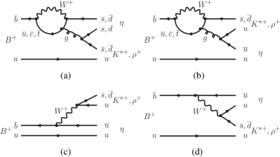
Figure 1: Feynman diagrams for $B^{+}\to\eta K^{*+}$ and $\eta\rho^{+}$ decays. The corresponding neutral decays are similar except that the spectator quark becomes a $d$ and (b) and (c) diagrams do not exist.

In the standard model, direct $CP$ violation (DCPV) occurs in decays due to interference between two (or more) amplitudes that have different strong and weak phases. The partial rate asymmetry can be written as

$${\mathcal{A}}_{CP}(B\to f)={\Gamma({\overline{B}\to\bar{f}})-\Gamma({B\to f})\over\Gamma({\overline{B}\to\bar{f}})+\Gamma({B\to f})}$$

$$={2|M_{1}||M_{2}|\sin\Delta\delta\sin\Delta\phi\over|M_{1}|^{2}+|M_{2}|^{2}+2|M_{1}||M_{2}|\cos\Delta\delta\cos\Delta\phi},$$ (1)

where $\overline{B}$ and $\bar{f}$ are the $CP$-conjugate states, and $\Delta\delta$ ($\Delta\phi$) is the difference of the strong (weak) phases between amplitudes $M_{1}$ and $M_{2}$. Here, the amplitude $M_{1}$($M_{2}$) represents the sum of the amplitudes from penguin (tree) diagrams having a common weak phase. The asymmetry will be sizable when the two type of amplitudes are of comparable strength with significant phase differences. However, $B\to\eta K^{*}$ and $B\to\eta\rho$ decay rates are expected to be dominated by penguin diagrams for $\eta K^{*}$ and tree diagrams for $\eta\rho$, so ${\mathcal{A}}_{CP}$ is expected to be small. On the other hand, amplitudes arising from new physics may interfere with these SM amplitudes to generate a sizable ${\mathcal{A}}_{CP}$ value. The experimental results BABARETA suggest that DCPV is small, albeit with large statistical uncertainties.

II Data Set and Apparatus

This analysis is based on a data sample collected at the $\Upsilon$(4S) resonance with the Belle detector BelleNIM at the KEKB kekb accelerator. The data sample corresponds to an integrated luminosity of $414\,{\rm fb}^{-1}$ and contains $449\times 10^{6}$ $B\overline{B}$ pairs.

The Belle detector is designed to measure charged particles and photons with high efficiency and precision. Charged particle tracking is provided by a silicon vertex detector (SVD) and a central drift chamber (CDC) that surround the interaction region. The charged particle acceptance covers the laboratory polar angle between $\theta=17^{\circ}$ and $150^{\circ}$, measured from the $z$ axis that is aligned anti-parallel to the positron beam. Charged hadrons are distinguished by combining the responses from an array of silica aerogel Cherenkov counters (ACC), a barrel-like array of 128 time-of-flight scintillation counters (TOF), and $dE/dx$ measurements in the CDC. The combined response provides $K/\pi$ separation of at least $2.5\sigma$ for laboratory momentum up to 3.5 GeV/$c$. Electromagnetic showers are detected in an array of 8736 CsI(Tl) crystals (ECL) located inside the magnetic volume, which covers the same solid angle as the charged particle tracking system. The 1.5-T magnetic field is contained via a flux return that consists of 4.7 cm thick steel plates, interleaved with resistive plate counters used for tracking muons. Two inner detector configurations were used. A 2.0 cm beampipe and a 3-layer silicon vertex detector were used for the first sample of $152\times 10^{6}$ $B\overline{B}$ pairs, while a 1.5 cm beampipe, a 4-layer silicon detector and a small-cell inner drift chamber were used to record the remaining $297\times 10^{6}$ $B\overline{B}$ pairs SVD2 .

We calculate the acceptance and study backgrounds using Monte Carlo (MC) simulation. For these simulation studies, the signal events, generic $b\to c$ decays and charmless rare $B$ decays are generated with the EVTGEN evtgen event generator. The continuum MC events are generated with the $e^{+}e^{-}\to\gamma^{*}\to q\bar{q}$ process in the JETSET jetset generator. The GEANT3 geant package is used for detector simulation.

III Event Selection and Reconstruction

Hadronic events are selected based on the charged track multiplicity and total visible energy sum, which give an efficiency greater than 99% for $B\overline{B}$ events. All primary charged tracks are required to be consistent with coming from the run-dependent interaction point within $\pm 2\,{\rm cm}$ along the $z$ axis and within $\pm 1.5\,{\rm cm}$ in the transverse plane. Particle identification (PID) is based on the likelihoods ${\mathcal{L}_{\rm K}}$ and ${\mathcal{L}_{\pi}}$ for charged kaons and pions, respectively. These likelihoods are calculated from CDC, TOF, and ACC information. A higher value of ${\mathcal{L}_{\rm K}}$/(${\mathcal{L}_{\pi}+\mathcal{L}_{\rm K}}$) indicates a more kaon-like particle. In this analysis, PID cuts are applied to all charged particles except those associated with $K^{0}_{S}\to\pi^{+}\pi^{-}$ decays. Unless explicitly specified, the PID cuts are ${\mathcal{L}_{\rm K}}$/(${\mathcal{L}_{\pi}+\mathcal{L}_{\rm K}}$) $>0.6$ for kaons and $<0.4$ for pions. The corresponding efficiencies are $85$% for kaons and $89$% for pions; $8$% of pions are misidentified as kaons and $11$% of kaons are misidentified as pions.

We form $\pi^{0}$ candidates from photon pairs with an invariant mass between 118 MeV/$c^{2}$ and $150\,{\rm MeV}/c^{2}$ ($2.5\sigma$). The photon energies must exceed 50 MeV, and the $\pi^{0}$ momentum in the center-of-mass (CM) frame must exceed 0.35 GeV/$c$. $K_{S}^{0}$ candidates are reconstructed from pairs of oppositely charged tracks whose invariant mass lies within $\pm 10\,{\rm MeV}/c^{2}$ ($2.5\sigma$) of the $K_{S}^{0}$ meson mass. We also require that the vertex of the $K^{0}_{S}$ be well-reconstructed and displaced from the interaction point, and that the $K^{0}_{S}$ momentum direction be consistent with the $K^{0}_{S}$ flight direction.

III.1 $\eta$ Meson Reconstruction

Candidate $\eta$ mesons are reconstructed in the $\eta\to\gamma\gamma$ and $\eta\to\pi^{+}\pi^{-}\pi^{0}$ modes. If one of the photons from the former $\eta$ decay mode can be paired with another photon and have a reconstructed $\gamma\gamma$ mass within $3\sigma$ of the $\pi^{0}$ meson mass, the $\eta$ candidate is discarded. We relax the PID requirement for charged pions from the latter $\eta$ decay mode to ${\mathcal{L}_{\rm K}}$/(${\mathcal{L}_{\pi}+L_{\rm K}}$) $<0.9$. Candidate $\eta$ mesons are required to satisfy the following mass selections: $500$ MeV/$c^{2}$$\leq M_{\gamma\gamma}\leq 575$ MeV/$c^{2}$ and $537$ MeV/$c^{2}$$\leq M_{\pi^{+}\pi^{-}\pi^{0}}\leq 557$ MeV/$c^{2}$, where the reconstructed mass resolutions are 12 MeV/$c^{2}$ for $\eta\to\gamma\gamma$ and 3.5 MeV/$c^{2}$ for $\eta\to\pi^{+}\pi^{-}\pi^{0}$. When reconstructing the $B$ meson candidate, the momentum of the $\eta$ candidate is recalculated by applying the $\eta$ mass constraint. The $\eta\to\gamma\gamma$ candidates must satisfy $|\cos\theta^{*}|<0.90$, where $\theta^{*}$ is the angle between the photon direction and the direction of the CM frame in the $\eta$ rest frame; this requirement suppresses soft photon combinatorial and $B\to K^{*}\gamma$ feed-across backgrounds.

III.2 $K^{*}$ and $\rho$ Meson Reconstruction

$K^{*0}$ candidates are reconstructed from $K^{+}\pi^{-}$ and $K_{S}^{0}\pi^{0}$ pairs, while the $K^{*+}$ candidates are reconstructed from $K^{+}\pi^{0}$ and $K_{S}^{0}\pi^{+}$ pairs. These candidates are required to have reconstructed masses within $\pm$75 MeV/$c^{2}$ of the nominal value PDG . Candidate $\rho^{0}$ ($\rho^{+}$) mesons are reconstructed from $\pi^{-}\pi^{+}$ ($\pi^{0}\pi^{+}$) pairs. Each combination is required to have a reconstructed mass within $\pm$150 MeV/$c^{2}$ of the nominal value PDG .

III.3 $B$ Meson Reconstruction

The $B$ meson candidates are reconstructed from $\eta K^{*0}$, $\eta K^{*+}$, $\eta\rho^{0}$, and $\eta\rho^{+}$ combinations. They are characterized by the beam-energy-constrained mass $M_{\rm bc}$ = $\sqrt{E^{2}_{\rm beam}/c^{4}-|P_{B}/c|^{2}}$ and the energy difference $\Delta E=E_{B}-E_{\rm beam}$, where $E_{\rm beam}=5.29$ GeV, and $P_{B}$ and $E_{B}$ are the momentum and energy, respectively, of the $B$ candidate in the CM frame. We define the fit region in the $M_{\rm bc}$–$\Delta E$ plane as $M_{\rm bc}>5.2\,{\rm GeV}/c^{2}$ and $|\Delta E|<0.25\,{\rm GeV}$. We define the signal region as the overlap of the bands $M_{\rm bc}>5.27\,{\rm GeV}/c^{2}$ and $|\Delta E|<0.05\,{\rm GeV}$.

From signal MC, we find that $8-10$% of the events contain multiple $B$ candidates. Only one $B$ candidate per event is retained for the likelihood fit. If there are multiple $\eta$ candidates, we choose the one with the smallest $\chi^{2}$ of the fit with a mass (vertex and mass) constraint to the kinematics of the $\eta$ meson in the case of $\eta\to\gamma\gamma$ ($\eta\to\pi^{+}\pi^{-}\pi^{0}$) decays. Among the $B$ candidates made of the same $\eta$ candidate, we choose the one with the smallest vertex $\chi^{2}$ in the cases of $K^{*0}\to K^{+}\pi^{-}$ or $\rho^{0}\to\pi^{+}\pi^{-}$; or then the one with the mass closest to nominal in the case of $K^{*+}\to K^{0}\pi^{+}$; or then the $\pi^{0}$ mass closest to the nominal in all other cases.

IV Background Suppression

The dominant background for exclusive two-body $B$ decays comes from the $e^{+}e^{-}\to\gamma^{*}\to q\bar{q}$ continuum ($q=u,\,d,\,s,\,c$), which has a jet-like event topology in contrast to more spherical $B\overline{B}$ events. The other major backgrounds involve feed-across from these and other charmless $B$ decays. The background from $b\to c$ decays has a small impact because the $M_{\rm bc}$ and $\Delta E$ distributions do not peak in the signal region. In this analysis, the fit does not distinguish non-resonant $B\to\eta K\pi$ decays from $B\to\eta K^{*}$ decays, since they have the same $M_{\rm bc}$ and $\Delta E$ distributions. The non-resonant contribution is estimated and subtracted independently using the $K\pi$ invariant mass distributions of the fitted $B$-decay yields.

IV.1 Continuum Background

Signal and continuum events are distinguished in two steps. Here, all the variables are calculated in the CM frame. First, we require $|\cos\theta_{T}|<0.9$, where $\theta_{T}$ is defined as the angle between the $\eta$ direction of a $B$ candidate and the thrust axis from all particles in the event not associated with that $B$ candidate. This retains 90% of signal and removes $\sim$56% of continuum. Second, a likelihood ${\cal L}_{s}$ (${\cal L}_{c}$) for signal (continuum) is formed from two independent variables—$\cos\theta_{B}$, where $\theta_{B}$ is the polar angle of the $B$ candidate momentum direction, and a Fisher discriminant fisher ${\cal F}=\vec{\alpha}\cdot\vec{R}$ that combines seven event shape variables: $\cos\theta_{T}$, $S_{\perp}$(the sum of the magnitudes of the momenta transverse to the $\eta$ direction for all particles more than $45^{\circ}$ away from the $\eta$ axis, divided by the sum of the magnitudes of the momenta of all particles not from the candidate $B$ meson sperp ), and the five modified Fox-Wolfram moments fw $R_{2}^{so}$, $R_{4}^{so}$, $R_{2}^{oo}$, $R_{3}^{oo}$, and $R_{4}^{oo}$. The Fisher discriminant’s weight vector $\vec{\alpha}$ is determined to maximize the separation between signal events and continuum background using MC data; these Fox-Wolfram moments are used since they are not correlated with $M_{\rm bc}$. The likelihood ratio ${\cal R}={\cal L}_{s}/({\cal L}_{s}+{\cal L}_{c})$, which peaks near one for signal and near zero for continuum, is used to distinguish signal from continuum.

The distribution of ${\cal R}$ is found to depend somewhat on the event’s $B$ flavor tagging quality parameter $r$ btag , which ranges from zero for no flavor identification to unity for unambiguous flavor assignment. We partition the data into three $r$ regions, $r\leq 0.5$, $0.5<r\leq 0.75$, and $r>0.75$. In each $r$ region, the optimal cut on ${\cal R}$ is determined by maximizing the significance $N_{S}/\sqrt{N_{S}+N_{B}}$, where $N_{S}$ and $N_{B}$ are the retained number of signal and continuum background events selected in MC samples. For cut optimization studies, we assume the branching fractions of $2.0\times 10^{-5}$ for $\eta K^{*}$, $5.0\times 10^{-6}$ for $\eta\rho^{+}$, and $1.0\times 10^{-6}$ for $\eta\rho^{0}$. For $B^{0}\to\eta K^{*0},\eta\to\gamma\gamma,K^{*0}\to K^{+}\pi^{-}$ decays, a typical cut of ${\mathcal{R}}>0.4$ is $\sim 87$% efficient for signal and removes $\sim 67$% of the continuum background for data in the region $r\leq 0.5$, and a cut of ${\mathcal{R}}>0.2$ is $\sim 94$% efficient for signal and removes $\sim 53$% of the continuum background for data in the region $r>0.75$.

IV.2 Backgrounds from $B$ Decays

$B\to K^{*}(\rho)\gamma$ is the dominant charmless $B$-decay background for $B\to\eta K^{*}(\rho)$, $\eta\to\gamma\gamma$ decays. The $\eta\to\gamma\gamma$ selection, $|\cos\theta^{*}|<0.90$, removes 85% of this background. To further suppress it, we pair each photon from the $\eta\to\gamma\gamma$ candidate with the $K^{*}$ or $\rho$ candidate and reject those events where $M_{\rm bc}>5.27\,{\rm GeV}/c^{2}$ and $-0.2\,{\rm GeV}<\Delta E<0.1\,{\rm GeV}$. We thus remove 96% of this background and retain 93% of the signal events. For $B\to\eta\rho$ decays, a measurable contribution from other charmless $B$ and $b\to c$ decays remains (see Table  1). The contributions of these backgrounds are taken into account in the analysis.

Table 1: Estimated $B-decay$ background contributions in the fit region to $B\to\eta\rho$ from $b\to c$ ($N_{\rm bc}$), charmless $B$ decay ($N_{\rm r}$), and $\eta K^{*}$ feed-across ($N_{\rm feed}$) and measured yields from all sources ($N$) but dominated by residual continuum background, after application of the $\cos\theta_{T}$ and ${\mathcal{R}}$ cuts. $N_{\rm bc}$ and $N_{\rm r}$ are estimated from MC samples.

Mode	$N_{\rm bc}$	$N_{\rm r}$	$N_{\rm feed}$	$N$
$\eta_{\gamma\gamma}\rho^{0}$	$62$	$81$	$17$	$2931$
$\eta_{\pi\pi\pi^{0}}\rho^{0}$	$67$	$27$	$5$	$1063$
$\eta_{\gamma\gamma}\rho^{+}$	$148$	$74$	$3$	$4169$
$\eta_{\pi\pi\pi^{0}}\rho^{+}$	$76$	$22$	$1$	$1809$

V Analysis Procedure

Signal yields are obtained using an extended unbinned maximum likelihood fit to the $M_{\rm bc}$ and $\Delta E$ distributions (2-D ML) for events that satisfy the $\cos\theta_{T}$ and ${\cal R}$ requirements.

For $N$ input candidates, the likelihood is defined as

$$L =\frac{e^{-(N_{S}+N_{qq}+N_{\rm bc}+N_{\rm r}+N_{\rm feed})}}{N!}\prod_{i=1}^{N}(N_{S}P_{S_{i}}+$$ (2)

$$N_{qq}P_{{qq}_{i}}+N_{\rm bc}P_{{\rm bc}_{i}}+N_{\rm r}P_{{\rm r}_{i}}+N_{\rm feed}P_{{\rm feed}_{i}}),$$

where $P_{S_{i}}$, $P_{{qq}_{i}}$, $P_{{\rm bc}_{i}}$, $P_{{\rm r}_{i}}$ and $P_{{\rm feed}_{i}}$ are the probability density functions for event $i$, with measured values $M_{{\rm bc},i}$ and $\Delta E_{i}$, to arise from signal, continuum background, $b\to c$ background, charmless $B$ decay background, and feed-across background, respectively. The small yields $N_{\rm bc}$, $N_{\rm r}$, and $N_{\rm feed}$ are fixed from the MC analysis.

The continuum, $b\to c$ and charmless $B$-decay background $\Delta E$ probability density functions (PDF) are modeled by second- or third-order polynomial functions. The continuum and $b\to c$ background components in $M_{\rm bc}$ are modeled by a smooth function argus . To account for the peaking behavior of $M_{\rm bc}$ in the signal region from charmless $B$ decay backgrounds, we use the sum of two bifurcated-Gaussian functions to model the distributions. The bifurcated Gaussian combines the left half of a wide-resolution Gaussian with the right half of a narrow-resolution Gaussian, both having a common mean. For $B\to\eta\rho$ decays, the $M_{\rm bc}$ and $\Delta E$ distributions from $\eta K^{*}$ feed-across will behave like signal with a $\Delta E$ shift of $-50$ MeV. The PDF shape for each contribution is determined from MC. The first-order coefficient of the continuum-background $\Delta E$ polynomial and the parameters of the $M_{\rm bc}$ function are allowed to float in each fit.

For the signal $\Delta E$ distribution, we combine two bifurcated-Gaussian functions. The first accounts for $60$-$80$% of the total area and the wider second models the low-energy tail. $M_{\rm bc}$ is weakly correlated with $\Delta E$, so we construct separate bifurcated Gaussians for $M_{\rm bc}$ in the three ranges $|\Delta E|<0.05\,{\rm GeV}$, $0.05\,{\rm GeV}<|\Delta E|<0.1\,{\rm GeV}$, and $0.1\,{\rm GeV}<|\Delta E|<0.25\,{\rm GeV}$. The parameters of these functions are estimated from MC first, then calibrated with a large control sample of $B^{+}\to\vbox{\halign{#\cr\hrulefill$\smash{\phantom{\scriptstyle 0}}$\crcr\kern-1.0pt\nointerlineskip\vskip 1.07639pt\cr$\hfil{D}^{0}\hfil$\crcr}}\pi^{+}$, $\vbox{\halign{#\cr\hrulefill$\smash{\phantom{\scriptstyle 0}}$\crcr\kern-1.0pt\nointerlineskip\vskip 1.07639pt\cr$\hfil{D}^{0}\hfil$\crcr}}\to K^{+}\pi^{-}\pi^{0}$ decays.

For decays with more than one sub-decay process, the final results are obtained by fitting the sub-decay modes simultaneously with the expected efficiencies folded in and with the branching fraction as the common output. The statistical significance ($\Sigma$) of the signal is defined as $\sqrt{-2\ln(L_{0}/L_{\rm max})}$, where $L_{0}$ and $L_{\rm max}$ denote the likelihood values for zero signal events and the best fit numbers, respectively.

The 90% confidence level (C.L.) upper limit $x_{90}$ on the signal yield is calculated from the equation

$$\frac{\int_{0}^{x_{90}}L(x)\,dx}{\int_{0}^{\infty}L(x)\,dx}=90\%\,.$$

To incorporate the systematic uncertainty in the calculation of $x_{90}$, the likelihood function is smeared with a Gaussian function with the resolution from the systematic uncertainty. That smeared likelihood function is also used to calculate the significance of the signal including the systematic uncertainty.

VI Measurements of Branching Fractions

VI.1 Efficiencies and Corrections

The overall reconstruction efficiency $\epsilon$ is first obtained using MC samples and then multiplied by PID efficiency corrections obtained from data. The PID efficiency correction is determined using $D^{*+}\to D^{0}\pi^{+}$, $D^{0}\to K^{-}\pi^{+}$ data samples. Other MC efficiency corrections are determined by comparing data and MC predictions for other well-known processes. The charged-particle tracking efficiency correction is studied using a high-momentum $\eta$ sample and is determined by comparing the ratios of $\eta\to\pi^{+}\pi^{-}\pi^{0}$ to $\eta\to\gamma\gamma$ in data and MC. The same high-momentum $\eta$ sample is also used for $\pi^{0}$ reconstruction efficiency corrections by comparing the ratio of $\eta\to\pi^{0}\pi^{0}\pi^{0}$ to $\eta\to\gamma\gamma$ between the data and MC sample. The $K^{0}_{S}$ reconstruction efficiency is verified by comparing four $K^{*}(892)$ decay channels ($K^{+}\pi^{-}$, $K^{+}\pi^{0}$, $K^{0}_{S}\pi^{+}$, $K^{0}_{S}\pi^{0}$) in inclusive $K^{*}$ and exclusive $B\to J/\psi K^{*}$ samples. The ${\mathcal{R}}$ cut efficiency correction is determined using $B^{+}\to\vbox{\halign{#\cr\hrulefill$\smash{\phantom{\scriptstyle 0}}$\crcr\kern-1.0pt\nointerlineskip\vskip 1.07639pt\cr$\hfil{D}^{0}\hfil$\crcr}}\pi^{+}$ decays. For $\eta$ and $K^{*}$ reconstruction and mass cuts, we use the high-momentum $\eta$ and $K^{*}$ sample for the efficiency correction studies. The above studies show good agreement between data and MC; the reconstruction and selection efficiencies differ by about $2$%. The PID, $\pi^{0}$, $\eta$ and $K^{*}$ reconstruction efficiency corrections are applied and the systematic uncertainties are also obtained from the above studies.

Table 2: Summary of results for each channel listed in the first column. The measured signal yield ($N_{S}$), reconstruction efficiency ($\epsilon$), total efficiency ($\epsilon_{\rm{tot}}$) including the secondary branching fraction, statistical significance ($\Sigma$) and measured branching fractions are shown. Uncertainties shown in second and sixth columns are statistical only. For the final combined branching fractions, corrections for contributions from non-resonant or higher resonance components have been applied. The total systematic uncertainties are given, and the combined significances include the systematic uncertainties.

Mode	$N_{S}$	$\epsilon$(%)	$\epsilon_{\rm{tot}}$(%)	$\Sigma$	${\mathcal{B}}(10^{-6})$
$\eta_{\gamma\gamma}K^{*0}_{K^{+}\pi^{-}}$	$336.2^{+30.1}_{-29.2}$	$16.9$	$4.4$	$14.2$	$16.9\pm 1.5$
$\eta_{\pi\pi\pi^{0}}K^{*0}_{K^{+}\pi^{-}}$	$93.4^{+14.6}_{-13.8}$	$9.8$	$1.5$	$8.7$	$14.1^{+2.2}_{-2.1}$
$\eta_{\gamma\gamma}K^{*0}_{K^{0}\pi^{0}}$	$20.1^{+7.5}_{-6.7}$	$2.1$	$0.27$	$3.6$	$16.7^{+6.3}_{-5.6}$
$\eta_{\pi\pi\pi^{0}}K^{*0}_{K^{0}\pi^{0}}$	$9.5^{+5.0}_{-4.2}$	$1.3$	$0.098$	2.6	$21.6^{+11.5}_{-9.7}$
$\eta K^{*0}$	-	-	-	$15.7$	$15.2\pm 1.2\pm 1.0$
$\eta_{\gamma\gamma}K^{*+}_{K^{+}\pi^{0}}$	$79.8^{+16.1}_{-15.3}$	$6.7$	$0.88$	6.1	$20.1^{+4.1}_{-3.9}$
$\eta_{\pi\pi\pi^{0}}K^{*+}_{K^{+}\pi^{0}}$	$24.1^{+8.7}_{-7.9}$	$4.2$	$0.32$	$3.5$	$16.9^{+6.1}_{-5.6}$
$\eta_{\gamma\gamma}K^{*+}_{K^{0}\pi^{+}}$	$120.3^{+16.2}_{-15.4}$	$4.5$	$1.2$	$10.1$	$22.6^{+3.1}_{-2.9}$
$\eta_{\pi\pi\pi^{0}}K^{*+}_{K^{0}\pi^{+}}$	$29.2^{+7.3}_{-6.6}$	$2.6$	$0.38$	$6.2$	$16.9^{+4.3}_{-3.8}$
$\eta K^{*+}$	-	-	-	$12.3$	$19.3^{+2.0}_{-1.9}\pm 1.5$
$\eta_{\gamma\gamma}\rho^{0}$	$19.5^{+11.3}_{-10.4}$	$8.9$	$3.5$	$2.1$	$1.25^{+0.73}_{-0.67}$
$\eta_{\pi\pi\pi^{0}}\rho^{0}$	$0.9^{+4.6}_{-3.9}$	$5.5$	$1.2$	$0.2$	$0.17^{+0.84}_{-0.66}$
$\eta\rho^{0}$	-	-	-	$1.3$	$0.84^{+0.56}_{-0.51}\pm 0.19$
$\eta_{\gamma\gamma}\rho^{+}$	$38.1^{+16.1}_{-15.2}$	$5.5$	$2.2$	$2.6$	$3.9^{+1.7}_{-1.6}$
$\eta_{\pi\pi\pi^{0}}\rho^{+}$	$15.8^{+8.9}_{-8.0}$	$3.50$	$0.79$	2.1	$4.4^{+2.5}_{-2.2}$
$\eta\rho^{+}$	-	-	-	$2.7$	$4.1^{+1.4}_{-1.3}\pm 0.4$

VI.2 Fit Results

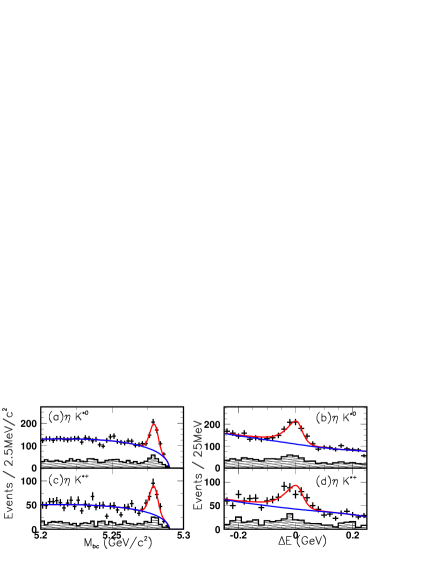
Figure 2: Projections on $M_{\rm bc}$ (for the signal slice in $\Delta E$) and $\Delta E$ (for the signal slice in $M_{\rm bc}$) for $\eta K^{*0}$ (a,b) and $\eta K^{*+}$ (c,d) with the expected signal and background curves overlaid. The shaded area represents $\eta\to\pi^{+}\pi^{-}\pi^{0}$ decays.

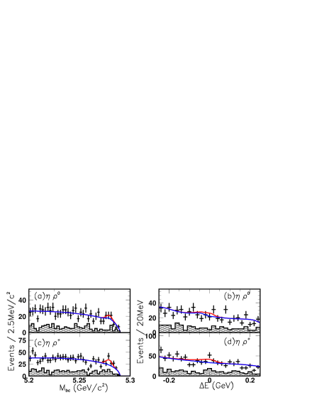
Figure 3: Projections on $M_{bc}$ (for the signal slice in $\Delta E$) and $\Delta E$ (for the signal slice in $M_{\rm bc}$) from 2-D ML fit results for $\eta\rho^{0}$ (a,b) and $\eta\rho^{+}$ (c,d) with the expected signal and background curves overlaid. The shaded area represents $\eta\to\pi^{+}\pi^{-}\pi^{0}$ decays.

The fitted signal yields and branching fractions are shown in Table 2. Several consistency checks are made, including tighter ${\mathcal{R}}$ cuts as well as 1-D ML $M_{\rm bc}$ and $\Delta E$ fits, and they are all found to be consistent. The total observed yields are $N_{\eta K^{*0}}=459.2^{+34.6}_{-33.3}$ for $B^{0}\to\eta K^{*0}$, $N_{\eta K^{*+}}=253.4^{+25.5}_{-24.0}$ for $B^{+}\to\eta K^{*+}$, $N_{\eta\rho^{0}}=20.4^{+12.2}_{-11.0}$ for $B^{0}\to\eta\rho^{0}$ and $N_{\eta\rho^{+}}=53.9^{+18.4}_{-17.1}$ for $B^{+}\to\eta\rho^{+}$. Figure 2 shows the projections of the data and the fits onto $M_{\rm bc}$ (for events in $\Delta E$ signal slice) and $\Delta E$ (for events in the $M_{\rm bc}$ signal slice) for the $B\to\eta K^{*}$ decays, while Fig. 3 shows the corresponding projections for the $B\to\eta\rho$ decays.

VI.3 Non $K^{*}(892)$ Components

The background-subtracted $K^{*}$ helicity distributions within the $M_{\rm bc}$ and $\Delta E$ signal regions (Fig. 4) are consistent with the expectation from $\eta K^{*}$ decays, indicating no significant S-wave or higher resonance contribution in the $K^{*}$ mass region. The $K^{*0}(K^{*+})$ helicity angle ($\theta_{\rm{hel}}$) is the angle between the $\pi^{-}(\pi^{0},K^{0})$ direction and the opposite of the $B$ direction in the $K^{*}$ rest frame. The binned $\chi^{2}$ per degree of freedom is $\chi^{2}/N=9.7/10$ for $K^{*0}$ and $\chi^{2}/N=3.6/10$ for $K^{*+}$.

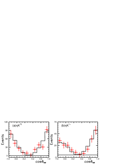
Figure 4: Distributions of the $K^{*}$ helicity for the (a) $K^{*0}$ and (b) $K^{*+}$ modes in case of $B\to\eta K^{*}$ decays. The overlaid histograms represent the distributions from MC normalized by the 2-D fit results.

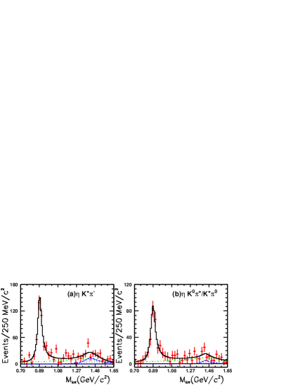
Figure 5: Fitted yields vs. the $K\pi$ invariant mass for the (a) $(K\pi)^{0}$ and (b) $(K\pi)^{+}$ modes. The overlaid functions are the results of a binned $\chi^{2}$ fit. The dashed line represents the contribution from the D-wave $K_{2}^{*}(1430)$, and the dot-dash line represents the LASS S-wave parameterization. LASS parameterization parameters, widths of P-wave and D-wave functions are allowed to float in the fits.

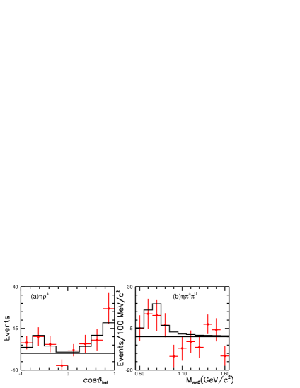
Figure 6: Fitted yields vs. (a) $\rho^{+}$ helicity and (b)$\pi^{+}\pi^{0}$ invariant mass from $B\to\eta\rho^{+}$ decays. The overlaid histograms are expected distributions from MC and normalized by the 2-D fit results with $\chi^{2}/N=6.8/8$ for (a) and $\chi^{2}/N=13.6/11$ for (b).

We use a 2D-ML fit to the $K\pi$ invariant mass distributions to evaluate the small S-wave or higher resonance $K\pi$ contaminations in the $K^{*}$ mass region. A clear excess in the higher $K\pi$ invariant mass region is observed (Fig. 5). To estimate these contributions, we fit the distributions with a P-wave relativistic Breit-Wigner function for the $K^{*}$(892), a D-wave relativistic Breit-Wigner function for the $K_{2}^{*}(1430)$ resonance and an ad hoc function for the S-wave contribution. Several functions are used to model the S-wave contribution in the $K\pi$ mass region $1.0$ GeV/$c^{2}$ to $1.5$ GeV/$c^{2}$, including a $K_{0}^{*}(1350)$ resonancelass , the LASS distributionlass , and a threshold function. The LASS distribution contains a non-resonant S-wave background function interfering with an S-wave $K_{0}^{*}(1430)$ resonance. Figure 5 shows one example of our fitting results with the S-wave contribution modeled by the LASS distribution. Based on these studies with various S-wave functions, the non-resonant $K\pi$ contributions are ($5.6\pm 3.0$)% for $\eta K^{*0}$ and ($5.0\pm 3.0$)% for $\eta K^{*+}$ decays. These corrections are applied to the final branching fraction measurements of $B\to\eta K^{*}$.

For $B^{+}\to\eta\rho^{+}$ decays, we examine the properties of the $\rho^{+}$ candidates through 2-D ML fits in bins of $\pi^{+}\pi^{0}$ invariant mass and $\rho^{+}$ helicity. Although statistically limited, a $\rho^{+}$ mass peak and a polarized $\rho^{+}$ helicity distribution are observed (Fig. 6) and are consistent with the expectation from $\eta\rho^{+}$. Due to the limited statistics for $B^{+}\to\eta\rho^{+}$ decays, a larger systematic error for the non-resonant or higher resonance contributions is assigned with no corrections applied.

VII Systematic Error

Systematic errors, enumerated in Table 3, arise from efficiency corrections, non-resonant corrections and fitting. The main sources of uncertainties in the efficiency corrections are from the reconstruction of low-momentum charged tracks, low-energy photon finding, and the ${\mathcal{R}}$ cut efficiency. The systematic errors include contributions of $1$% for ${\mathcal{R}}$ cuts, $1$% per reconstructed charged particle, $0.5$% for each charged particle identification, $4$% for $\pi^{0}$ reconstruction, $4.5$% for $K^{0}_{S}$ reconstruction, and $2$% for $\eta$ reconstruction with $\eta\to\gamma\gamma$. We use $B^{+}\to\vbox{\halign{#\cr\hrulefill$\smash{\phantom{\scriptstyle 0}}$\crcr\kern-1.0pt\nointerlineskip\vskip 1.07639pt\cr$\hfil{D}^{0}\hfil$\crcr}}\pi^{+}$ decays to estimate the uncertainties in the signal PDF’s used for fitting $M_{\rm bc}$ and $\Delta E$ by comparing the mean and the width of the $M_{\rm bc}$ and $\Delta E$ distributions between the $B^{+}\to\vbox{\halign{#\cr\hrulefill$\smash{\phantom{\scriptstyle 0}}$\crcr\kern-1.0pt\nointerlineskip\vskip 1.07639pt\cr$\hfil{D}^{0}\hfil$\crcr}}\pi^{+}$ data and the MC sample. In Table 3, “Fit” means the systematic uncertainty from the PDF function modeling. “$B_{s}$” means the systematic uncertainty from the braching fractions of $\eta$ and $K^{*}(\rho)$ decays, which is obtained from the PDG tables PDG . “Non-resonant” means the systematic uncertainty from the non-resonant or higher resonant contributions in the $K^{*}(\rho)$ mass window regions, which is obtained from the studies of a 2D-ML fit to the $K\pi$ invariant mass distribution. For MC estimated $b\to c$ and charmless $B$ decay backgrounds (“$N_{\rm bc}$” and “$N_{\rm r}$”, respectively), we vary the estimated yields by $\pm 50$% and refit the data. The difference between the resulting signal yield and the nominal value is taken as an additional systematic error. The overall relative systematic errors are $6.5$% for $\eta K^{*0}$, $7.5$% for $\eta K^{*+}$, $22.1$% for $\eta\rho^{0}$ and $9.6$% for $\eta\rho^{+}$.

Table 3: Relative systematic errors for $\eta K^{*}$ and $\eta\rho$. The unit is in percent $(\%)$.

Contribution	$\eta K^{*0}$	$\eta K^{*+}$	$\eta\rho^{0}$	$\eta\rho^{+}$
charged track/$K^{0}_{S}$ reconstruction	2.9	4.4	3.3	1.8
$\pi^{0}$/$\eta\to\gamma\gamma$ selection	2.8	3.5	3.2	4.8
$\eta$ mass window	2.0	2.0	2.0	2.0
$K^{*}(\rho)$ mass window	2.0	2.0	2.0	2.0
PID correction	1.3	1.0	1.6	0.8
$\mathcal{R}$ requirement	1.0	1.0	1.0	1.0
Fit	$1.7$	$1.8$	$7.5$	$4.2$
$N_{\rm bc}$, $N_{\rm r}$	$1.2$	$1.2$	$7.5$	$0.4$
$\eta K^{*}$ feed-across	-	-	$17.4$	$1.1$
$N_{B\overline{B}}$	1	1	1	1
$B_{s}$	1.0	1.0	1.4	0.8
Non-resonant	3.0	3.0	6.0	6.0
Total	$6.5$	$7.5$	$22.1$	$9.6$

VIII $\mathcal{A}_{CP}$ Measurements

We measure $\mathcal{A}_{CP}$ for $B\to\eta K^{*}$ and $B^{+}\to\eta\rho^{+}$. To account for the wrong-tag fraction $w$, the true value of $\mathcal{A}_{CP}$ is related to the measured $\mathcal{A}^{\rm obs}_{CP}$ via ${\mathcal{A}^{\rm obs}_{CP}}=(1-2w){\mathcal{A}_{CP}}$. Among the decay modes we study, only those in which the $\mathcal{A}_{CP}$ values are determined by low momentum charged pions have a significant $w$: the wrong-tag fractions for $K^{*+}\to K^{0}\pi^{+}$ is $\sim 1.5$% for $\eta K^{*+}$ decays and $\sim 2.0$% for $\eta\rho^{+}$ decays, while other decays have $w<0.1$%. Since the result for $\eta K^{*+}$ is obtained from a simultaneous fit to all four sub-decay modes with roughly equal statistics for $K^{*+}\to K^{+}\pi^{0}$ and $K^{*+}\to K^{0}\pi^{+}$, the wrong-tag effect for $\mathcal{A}_{CP}$ is less than 0.7%. Therefore, the only mode where we apply a correction due to the wrong tag fraction is $B^{+}\to\eta\rho^{+}$, where we estimate $w=2$%. To incorporate the $CP$ asymmetry in the fit, the coefficients of the signal and continuum background PDF’s in the likelihood are modified as follows: $N_{S}\to{1\over 2}N_{S}(1-q{\cal A}_{CP}^{\rm obs})$ and $N_{qq}\to{1\over 2}N_{qq}(1-q{\cal A}_{CP,qq})$, where $q=+1(-1)$ for a $B(\overline{B})$ meson tag and $\mathcal{A}^{\rm obs}_{CP}$,$\mathcal{A}_{CP,qq}$ are the $\mathcal{A}_{CP}$ outputs for signal and continuum, respectively. The results are ${\mathcal{A}^{\rm obs}_{CP}}(\eta K^{*0})=0.17\pm 0.08$, ${\mathcal{A}^{\rm obs}_{CP}}(\eta K^{*+})=0.03\pm 0.10$ and ${\mathcal{A}^{\rm obs}_{CP}}(\eta\rho^{+})=-0.04^{+0.34}_{-0.32}$.

Since the systematic errors in the reconstruction of the $\eta$ candidates and the number of $B\overline{B}$ events cancel in the ratio, the systematic uncertainty on $\mathcal{A_{CP}}$ comes mainly from the charge asymmetry in the identification of charged kaons and the fitting PDF’s. To estimated the fitting-PDF systematic uncertainty, we apply the same procedures as in the branching fraction measurements. The relative systematic errors from fitting PDF’s are estimated to be $3$% for $\eta K^{*0}$, $13$% for $\eta K^{*+}$, and $27$% for $\eta\rho^{+}$. The efficiency asymmetry for the PID of charged kaons is $0.01$ in absolute value.

IX Summary

In summary, we report measurements of the exclusive two-body charmless hadronic $B\to\eta K^{*}$ and $B\to\eta\rho$ decays with high statistics. Our results are consistent with previous measurements CLEO ; BABARETA and confirm that the branching fractions for $B^{0}\to\eta K^{*0}$ and $B^{+}\to\eta K^{*+}$ are large. The branching fractions obtained are ${\mathcal{B}}(B^{0}\to\eta K^{*0})=(15.2\pm 1.2\pm 1.0)\times 10^{-6}$, and ${\mathcal{B}}(B^{+}\to\eta K^{*+})=(19.3^{+2.0}_{-1.9}\pm 1.5)\times 10^{-6}$, where the first error is statistical and the second systematic. Our measurements indicate that the branching fraction for $B^{+}\to\eta K^{*+}$ is $1.4\sigma$ higher than that for $B^{0}\to\eta K^{*0}$. A $2.7\sigma$ excess is seen for $B^{+}\to\eta\rho^{+}$ decays. The branching fraction and 90% C.L. upper limits for $B\to\eta\rho$ decays are $\mathcal{B}$($B^{+}\to\eta\rho^{+}$)= $(4.1^{+1.4}_{-1.3}\pm 0.4)\times 10^{-6}$($<6.5\times 10^{-6}$) and $\mathcal{B}$($B^{0}\to\eta\rho^{0}$)$<1.9\times 10^{-6}$. The measurements of the $B\to\eta\rho$ branching fractions are consistent with theoretical predictions ali ; cheng ; pqcd ; rosner .

We have measured the direct $CP$ asymmetry in the $B\to\eta K^{*}$ and $B^{+}\to\eta\rho^{+}$ channels. Our results are ${\mathcal{A}_{CP}}(\eta K^{*0})=0.17\pm 0.08\pm 0.01,{\mathcal{A}_{CP}}(\eta K^{*+})=0.03\pm 0.10\pm 0.01$, and ${\mathcal{A}_{CP}}(\eta\rho^{+})=-0.04^{+0.34}_{-0.32}\pm 0.01$, all consistent with no asymmetry.

X Acknowledgments

We thank the KEKB group for the excellent operation of the accelerator, the KEK cryogenics group for the efficient operation of the solenoid, and the KEK computer group and the National Institute of Informatics for valuable computing and Super-SINET network support. We acknowledge support from the Ministry of Education, Culture, Sports, Science, and Technology of Japan and the Japan Society for the Promotion of Science; the Australian Research Council and the Australian Department of Education, Science and Training; the National Science Foundation of China and the Knowledge Innovation Program of the Chinese Academy of Sciences under contract No. 10575109 and IHEP-U-503; the Department of Science and Technology of India; the BK21 program of the Ministry of Education of Korea, the CHEP SRC program and Basic Research program (grant No. R01-2005-000-10089-0) of the Korea Science and Engineering Foundation, and the Pure Basic Research Group program of the Korea Research Foundation; the Polish State Committee for Scientific Research; the Ministry of Education and Science of the Russian Federation and the Russian Federal Agency for Atomic Energy; the Slovenian Research Agency; the Swiss National Science Foundation; the National Science Council and the Ministry of Education of Taiwan; and the U.S. Department of Energy.

References

(1)
CLEO Collaboration,
B.H. Behrens et al., Phys. Rev. Lett. 80, 3710 (1998);
S.J. Richichi et al., Phys. Rev. Lett. 85, 520 (2000).
(2)
Belle Collaboration,
P. Chang et al., Phys. Rev. D71, 091106(R) (2005).
(3)
BaBar Collaboration,
B. Aubert et al., Phys. Rev. Lett. 95, 131803 (2005);
B. Aubert et al., Phys. Rev. Lett. 97, 201802 (2006).
(4) A. Ali, G. Kramer, and C.-D. Lu,
Phys. Rev. D 58, 094009 (1998);
Xin Liu, Huisheng Wang, Zhenjun Xiao, Libo Guo and C.-D. Lu
Phys. Rev. D 73, 074002 (2006).
(5)Y.-H. Chen, H.-Y. Cheng, B. Tseng, and K.-C. Yang,
Phys. Rev. D 60, 094014 (1999); H.-Y. Cheng and K.C. Yang,
Phys. Rev. D 62, 054029 (2000).
(6)M.-Z. Yang and Y.D. Yang, Nucl. Phys. B 609, 469 (2001);
M. Beneke and M. Neubert, Nucl. Phys. B 651, 225 (2002);
D. Du, H. Gong, J. Sun, D. Yang, and G. Zhu,
Phys. Rev. D 65, 094025 (2002).
(7) M. Gronau and J.L. Rosner,
Phys. Rev. D 61, 073008 (2000);
C.-W. Chiang and J.L. Rosner, Phys. Rev. D 65, 074035 (2002);
C.-W. Chiang, M. Gronau, Z. Luo, J.L. Rosner and D.A. Suprun,
Phys. Rev. D 69, 034001 (2004).
(8) W.-S. Hou and K.-C. Yang, Phys. Rev. D 61,
073014 (2000).
(9)
Belle Collaboration, K. Abashian et al.,
Nucl. Instr. and Meth. A479, 117 (2002).
(10)
S. Kurokawa and E. Kikutani,
Nucl. Instr. and Meth. A499, 1 (2003),
and other papers therein.
(12)D.J. Lange,
Nucl. Instr. and Meth. A462, 152 (2001)
(13)T. Sjöstrand,
Comput. Phys. Commun.82, 74 (1994);
T. Sjöstrand and M. Bengston,
Comput. Phys. Commun.43, 367 (1987);
T. Sjöstrand, Comput. Phys. Commun.39, 347 (1986).
(14)R. Brun et al.,
GEANT 3.21, CERN Report DD/EE/84-1, 1984.
(15)
Particle Data Group, S. Eidelman et al.,
Phys. Lett. B 592, 1 (2004).
(16)
R.A. Fisher, Annals of Eugenics, 7, 179 (1936).
(17)
CLEO Collaboration, R. Ammar et al., Phys. Rev. Lett. 71, 674 (1993).
(18)The Fox-Wolfram moments were introduced in G.C. Fox
and S. Wolfram, Phys. Rev. Lett 41, 1581 (1978). The
modified Fox-Wolfram moments used in this paper is described
in C.H. Wang et al.(Belle Collaboration),
Phys. Rev. D 70, 012001 (2004) .
(19)
H. Kakuno et al., Nucl. Instr.and Meth. A533, 516 (2004).
(20)
H. Albrecht et al., Phys. Lett. B 241, 278 (1990).
(21)
LASS Collaboration, D. Aston et al., Nucl. Phys. B 296, 493 (1988).