Search for $B$ decays into $\eta^{\prime}\rho$, $\eta^{\prime}K^{*}$, $\eta^{\prime}\phi$, $\eta^{\prime}\omega$ and $\eta^{\prime}\eta^{(\prime)}$

Abstract

We report on a search for the exclusive two-body charmless hadronic $B$ meson decays $B\to\eta^{\prime}\rho$, $B\to\eta^{\prime}K^{*}$, $B^{0}\to\eta^{\prime}\phi$, $B^{0}\to\eta^{\prime}\omega$ and $B^{0}\to\eta^{\prime}\eta^{(\prime)}$. The results are obtained from a data sample containing 535 $\times 10^{6}$ $B\bar{B}$ pairs that were collected at the $\Upsilon(4S)$ resonance with the Belle detector at the KEKB asymmetric-energy $e^{+}e^{-}$ collider. We find no significant signals and report upper limits in the range $(0.5$–$6.5)\times 10^{-6}$ for all of the above decays.

I Introduction

Information on the two-body charmless hadronic $B$ meson decays with an $\eta^{\prime}$ meson in the final state ($B\to\eta^{\prime}h^{(*)}$) is incomplete at present. While the decay $B\to\eta^{\prime}K$ is observed with a large branching fraction, so far no other $B\to\eta^{\prime}h^{(*)}$ decay mode has been observed with greater than $5\sigma$ significance. The first evidence of $B\to\eta^{\prime}\pi$ has recently been reported  Aubert:2005bq ; Schuemann and BaBar found evidence for $B\to\eta^{\prime}K^{*}$ with larger than $4\sigma$ significance Aubert:2006as , and thus additional observations are expected in the near future. The study of these decay modes can improve the understanding of the flavor-singlet penguin amplitude with intermediate $t$, $c$ and $u$ quarks Chiang:2004nm . Furthermore, these studies increase our confidence in the reliability of a variety of other predictions, e.g, for the $CP$ violating parameter $\phi_{3}$ ($\gamma$), and are necessary to extract theory parameters such as the scalar penguin operator Chiang:2004nm ; Beneke:2003zv . Presently, theoretical predictions for the branching fractions of these decay modes cover the range (0.0001–7.6)$\times 10^{-6}$ Chiang:2004nm ; Beneke:2003zv ; Fu:2003fy . The most stringent upper limits for presently unobserved decays were reported by BaBar Aubert:2005bq ; Aubert:2006qd ; Aubert:2006as .

II Data set and apparatus

The study performed here includes the decays $B^{(0,+)}\to\eta^{\prime}\rho^{(0,+)}$, $B^{(0,+)}\to\eta^{\prime}K^{*(0,+)}$, $B^{0}\to\eta^{\prime}\phi$, $B^{0}\to\eta^{\prime}\omega$ and $B^{0}\to\eta^{\prime}\eta^{(\prime)}$ and is based on a data sample that contains 535 $\times 10^{6}$ $B\bar{B}$ pairs, collected with the Belle detector at the KEKB asymmetric energy $e^{+}e^{-}$ (3.5 GeV on 8 GeV) collider KEKB . Throughout this paper, the inclusion of the charge conjugate decay is implied unless stated otherwise.

KEKB operates at the $\Upsilon(4S)$ resonance ($\sqrt{s}=10.58$ GeV) with a peak luminosity that exceeds $1.7\times 10^{34}~{}{\rm cm}^{-2}{\rm s}^{-1}$. The Belle detector is a large-solid-angle magnetic spectrometer that consists of a silicon vertex detector (SVD), a 50-layer central drift chamber (CDC), an array of aerogel threshold Čherenkov counters (ACC), a barrel-like arrangement of time-of-flight scintillation counters (TOF), and an electromagnetic calorimeter comprised of CsI(Tl) crystals located inside a superconducting solenoid coil that provides a 1.5 T magnetic field. An iron flux-return located outside of the coil is instrumented to detect $K_{L}^{0}$ mesons and to identify muons. The detector is described in detail elsewhere Belle . Two inner detector configurations were used. A 2.0 cm beampipe and a 3-layer SVD were used for the first data sample of 152 $\times 10^{6}$ $B\bar{B}$ pairs (Set $I$), while a 1.5 cm beampipe, a 4-layer SVD and a small-cell inner drift chamber were used to record the remaining 383 $\times 10^{6}$ $B\bar{B}$ pairs (Set $II$)Ushiroda .

III Event selection and reconstruction

For what follows, unless stated otherwise, all variables are defined in the center-of-mass frame with the $z$ axis anti-parallel to the positron direction.

Charged hadrons are identified by combining information from the CDC ($dE/dx$), ACC and TOF systems. Both kaons and pions are selected with an average efficiency of 86% and are misidentified as pions or kaons, respectively, in 4% of the cases.

The $\eta^{\prime}$ mesons are reconstructed in the decays $\eta^{\prime}\to\eta\pi^{+}\pi^{-}$ (with $\eta\to\gamma\gamma)$ and $\eta^{\prime}\to\rho^{0}\gamma$, except for the decays $B^{0}\to\eta^{\prime}\eta$, $B^{0}\to\eta^{\prime}\eta^{\prime}$ and $B^{0}\to\eta^{\prime}\omega$, which use only the $\eta^{\prime}\to\eta\pi^{+}\pi^{-}$ channel. We define the $\eta^{\prime}$ ($h^{(*)}$) side as all particles involved in the decay of the $\eta^{\prime}$ ($h^{(*)}$) from the decay $B\to\eta^{\prime}h^{(*)}$. The $\eta$, $\rho^{0}$ and $\eta^{\prime}$ candidates on the $\eta^{\prime}$ side are reconstructed using the mass windows given in Table 1. Mass windows used to reconstruct the $h^{(*)}$ are given in Table 2. In addition, we require the following: photons originating from $\pi^{0}$ and $\eta$ decays are required to have energies of at least 100 MeV, photons from the $\eta^{\prime}$ in $\eta^{\prime}\to\rho^{0}\gamma$ have to be above 200 MeV in the laboratory frame. The transverse momenta of the $\pi^{\pm}$ for $\eta^{\prime}\to\eta_{\gamma\gamma}\pi^{+}\pi^{-}$ ($\eta^{\prime}\to\rho^{0}_{\pi^{+}\pi^{-}}\gamma$) candidates have to be greater than 100 MeV/$c$ (200 MeV/$c$). An additional requirement on the cosine of the $\rho^{0}$ helicity angle in $\eta^{\prime}\to\rho^{0}\gamma$ of $|\cos\theta_{h}|<0.85$ is applied, where $\theta_{h}$ is the angle between the momenta of one of the daughter pions of the $\rho^{0}$ and the $\eta^{\prime}$ in the $\rho^{0}$ rest frame. The vertex of the $K_{S}^{0}\to\pi^{+}\pi^{-}$ has to be displaced from the interaction point (IP) and the $K_{S}^{0}$ momentum direction must be consistent with its flight direction as indicated in Table 3 bib:ks .

Table 1: Invariant mass windows used to select intermediate states on the $\eta^{\prime}$ side. $\sigma$ denotes a standard deviation of the reconstructed mass distribution.

Mode	Mass window
	(MeV$/c^{2}$)	in units of $\sigma$
$\rho^{0}\to\pi^{+}\pi^{-}$	[550,870]	—
$\eta\to\gamma\gamma$	[500,570]	$+2.5/-3.3$
$\eta^{\prime}\to\eta\pi^{+}\pi^{-}$	[950,965]	$\pm 2.5$
$\eta^{\prime}\to\rho^{0}\gamma$	[941,970]	$\pm 2.5$

Table 2: Invariant mass windows used to select intermediate states on the $h^{(*)}$ side. $\sigma$ denotes a standard deviation of the reconstructed mass distribution.

Mode	Mass window
	(MeV$/c^{2}$)	in units of $\sigma$
$\pi^{0}\to\gamma\gamma$	[118,150]	$\pm 2.5$
$K_{S}^{0}\to\pi^{+}\pi^{-}$	[485,510]	$\pm 3$
$\rho^{+}\to\pi^{+}\pi^{0}$	[620,920]	—
$\rho^{0}\to\pi^{+}\pi^{-}$	[620,920]	—
$K^{*0}\to K^{+}\pi^{-}$	[820,965]	—
$K^{*+}\to K_{S}^{0}\pi^{+}$	[820,965]	—
$K^{*+}\to K^{+}\pi^{0}$	[820,965]	—
$\phi\to K^{+}K^{-}$	[1010,1030]	$\pm 3$
$\eta\to\gamma\gamma$	[510,575]	$\pm 2.5$
$\eta^{\prime}\to\eta\pi^{+}\pi^{-}$	[950,965]	$\pm 2.5$
$\omega\to\pi^{+}\pi^{-}\pi^{0}$	[750,810]	$\pm 2.5$

Table 3: Selection criteria for the distance of closest approach of one of the $K_{S}^{0}$ daughter pions to the IP ($dr$) in the $x$-$y$ plane, azimuthal angle between the momentum vector and the flight direction of the $K_{S}^{0}$ candidate inferred from the production and decay vertexes ($d\phi$), distance of closest approach between the two daughter tracks ($z$-dist.) and the flight length of the $K_{S}^{0}$ candidate in the $x$-$y$ plane ($fl$).

Momentum (GeV/$c$)	$dr$ (cm)	$d\phi$(rad)	$z$-dist. (cm)	$fl$ (cm)
$<0.5$	$>0.05$	$<0.3$	$<0.8$	—
$0.5-1.5$	$>0.03$	$<0.1$	$<1.8$	$>0.08$
$>1.5$	$>0.02$	$<0.03$	$<2.4$	$>0.22$

$B$ meson candidates are formed by combining an $\eta^{\prime}$ meson with one of the hadrons listed in Table 2 excluding $\pi^{0}$’s and $K_{S}^{0}$’s. $B$ candidates are identified using two kinematic variables: the energy difference, $\Delta E=E_{B}-E_{\mbox{\scriptsize beam}}$, and the beam-energy constrained mass, $M_{\mbox{\scriptsize bc}}=\sqrt{E_{\mbox{\scriptsize beam}}^{2}/c^{4}-(P_{B}/c)^{2}}$, where $E_{\mbox{\scriptsize beam}}$ is the beam energy and $E_{B}$ ($P_{B}$) is the reconstructed energy (momentum) of the $B$ candidate. Signal events peak at $\Delta E=0$ GeV and $M_{\mbox{\scriptsize bc}}=M_{B}$, where $M_{B}$ is the $B$ meson mass, with resolutions around $15$ MeV and $3$ MeV for $\Delta E$ and $M_{\mbox{\scriptsize bc}}$ respectively. An $\eta$ mass constraint fit is applied in the $\eta^{\prime}\to\eta\pi^{+}\pi^{-}$ subdecay in order to improve the $\Delta E$ resolution. Here the two photons from $\eta\to\gamma\gamma$ are constrained to have the nominal $\eta$ mass given by the Particle Data Group (PDG) bib:PDG04 . Events satisfying the requirements $M_{\mbox{\scriptsize bc}}>5.22$ GeV$/c^{2}$ and $|\Delta E|<0.25$ GeV are selected for further analysis. After all selections are applied, depending on the decay mode between 3% and 20% of the events have multiple $B$ candidates in one event. A $\chi^{2}$ variable is calculated to select the best candidate of such events. We select the $B$ with the smallest $\chi^{2}=\chi^{2}_{\text{vtx}}+\chi^{2}(M_{\eta^{\prime}})+\chi^{2}(M_{h^{(*)}})$, where $\chi^{2}_{\text{vtx}}$ is an estimator of the vertex quality for all charged particles not from the $K_{S}^{0}$ and $\chi^{2}(M_{X})=[(M_{X}-m_{X})/\sigma_{X}]^{2}$, where $M_{X}$ ($m_{X}$) is the reconstructed (nominal) mass of the particle candidate $X$ ($=$ $\eta^{\prime}$ or $h^{(*)}$) and $\sigma_{X}$ is the standard deviation of the reconstructed $X$ mass distribution as obtained from fits to MC distributions.

IV Background suppression

The dominant background for this analysis is continuum $e^{+}e^{-}\to q\bar{q}$ ($q=u,$ $d,$ $s,$ $c$). Other background sources are charmless $B$ decays such as $B\to\eta^{\prime}K$ and $b\to c$ decays. The background is 90% continuum with the remaining 10% nearly evenly split between the other two contributions.

Several event shape variables are used to distinguish the spherical $B\bar{B}$ topology from the jet-like $e^{+}e^{-}\to q\bar{q}$ continuum background. The thrust angle $\theta_{T}$ is defined as the angle between the $\eta^{\prime}$ momentum direction and the thrust axis formed by all particles not belonging to the reconstructed $B$ meson. Continuum events tend to peak near $|\cos\theta_{T}|=1$, while $B\bar{B}$ events have a uniform distribution. The requirement $|\cos\theta_{T}|<0.9$ is applied prior to all other event topology selections resulting in a signal efficiency (background reduction) of 90% (56%).

Additional continuum background suppression is obtained by using modified Fox-Wolfram moments SFW and $|\cos\theta_{B}|$, where $\theta_{B}$ is the angle between the flight direction of the reconstructed $B$ candidate and the beam axis. A Fisher discriminant (${\cal F}$) fisher:1936 is formed from a linear combination of $|\cos\theta_{T}|$, $S_{\perp}$ Ammar:1993sh and five modified Fox-Wolfram moments. $S_{\perp}$ is the ratio of the scalar sum of the transverse momenta of all tracks outside a $45^{\circ}$ cone around the $\eta^{\prime}$ direction to the scalar sum of their total momenta. The Fisher discriminant is then combined with the $B$ flight direction information to form an event topology likelihood function ${\cal L}_{S}$ (${\cal L}_{q\bar{q}}$), where the subscript $S$ ($q\bar{q}$) represents signal (continuum background). The signal over continuum background ratio varies over the range of the quality parameter $r$ of the $B$ flavor tagging of the accompanying $B$ meson. We use the standard Belle $B$ tagging algorithm TaggingNIM , which gives the $B$ flavor and the tagging quality $r$ ranging from zero for no flavor to unity for unambiguous flavor assignment. The data is divided into three $r$ regions and the likelihood ratio ${\cal R_{L}}={\cal L}_{S}/({\cal L}_{S}+{\cal L}_{q\bar{q}})$ requirements are determined to maximize $N_{S}/\sqrt{N_{B}}$, with $N_{S}$ ($N_{B}$) the expected number of signal (background), on Monte Carlo (MC) events in each $r$ region separately. More stringent selections are imposed for the first $r$ region at zero while looser criteria are used for $r$ close to one. More stringent selections are applied for decays with large continuum contribution such as $B\to\eta^{\prime}\rho$, while relatively clean decays such as $B^{0}\to\eta^{\prime}\phi$ have very loose requirements. The signal efficiencies (continuum background reduction) lie in the range of $42$%-$88$% ($98$%-$45$%).

Contributions from other charmless $B$ decays can contaminate the signal when a pion is misidentified as a kaon or when a random pion is added or missed. The dominant contribution for such misidentified events originates from $B\to\eta^{\prime}K$ decays. For the decays $B\to\eta^{\prime}\rho$, $B\to\eta^{\prime}K^{*}$ and $B^{0}\to\eta^{\prime}\omega$ the $B\to\eta^{\prime}K$ contamination is significant. For these decays we construct an alternative $B$ meson hypothesis assuming that it originates from a $B\to\eta^{\prime}K$ decay. We then veto an event if the alternative $\Delta E$ variable is within a decay-dependent window around $\Delta E=0$ GeV and $M_{\mbox{\scriptsize bc}}>5.27$ GeV/$c$. The selection is optimized for each decay and results in negligible signal suppression ($<0.5$%) while removing around 80% of the $B\to\eta^{\prime}K$ background.

V Measurement of branching fractions

The branching fractions are obtained using an extended unbinned maximum-likelihood fit to the $\Delta E$ and $M_{\mbox{\scriptsize bc}}$ distributions of selected events. This fit is performed simultaneously in the $\eta^{\prime}\to\eta\pi^{+}\pi^{-}$ and $\eta^{\prime}\to\rho^{0}\gamma$ subdecay channels for all $B$ decay modes, where applicable. In the case of $B^{+}\to\eta^{\prime}K^{*+}$ the two $K^{*+}$ subdecay modes (thus four subdecay channels in total) are fitted simultaneously. The extended likelihood function used is:

$$L(N_{S},N_{B_{j}}) = \frac{e^{-(N_{S}+\sum_{j}N_{B_{j}})}}{N!}\prod_{i=1}^{N}\biggl{[}N_{S}P_{S}(\Delta E_{i},M_{\mbox{\scriptsize bc}_{i}})$$ (1)

$$+\sum_{j}N_{B_{j}}P_{B_{j}}(\Delta E_{i},M_{\mbox{\scriptsize bc}_{i}})\biggr{]},$$

where $N_{S}$ ($N_{B_{j}}$) is the number of signal events (background events of source $j$) with probability density functions (PDFs) $P_{S}$ ($P_{B_{j}}$). The index $i$ runs from 1 to the total number of events $N$ in the selected sample.

The branching fraction ${\mathcal{B}}$ is determined by maximizing the combined likelihood for both data sets and all subdecays with ${\mathcal{B}}$ constrained to be the same for the subdecays. The number of signal events ($N_{S}$) for each decay mode is calculated by $N_{S}={\mathcal{B}}\,[N_{B\bar{B}}(I)\,\epsilon_{\text{t}}(I)+N_{B\bar{B}}(II)\,\epsilon_{\text{t}}(II)]$, where $N_{B\bar{B}}(k)$ is the number of $B\bar{B}$ produced for set $k=I$ or $II$ and $\epsilon_{\text{t}}(k)$ is the total reconstruction efficiency including subdecay branching fractions for set $k$.

The reconstruction efficiencies are determined from signal MC samples using the EvtGen package bib:Evtgen with final state radiation simulated by the PHOTOS package bib:Photos (thus measuring $B\to\eta^{\prime}h^{(*)}$$(\gamma)$). The efficiencies are calculated separately for Set $I$ and Set $II$. The absolute efficiency for Set $II$ is typically about 0.5% larger than for Set $I$ (for efficiencies averaged over the two sets see Tables 4 and 5). Corrections due to differences between data and MC are included for the charged track identification and photon, $\pi^{0}$ and $\eta$ reconstructions, resulting in an overall correction factor between $0.88$ and $0.99$ depending on the decay mode. We assume the numbers of $B^{+}B^{-}$ and $B^{0}\bar{B}{}^{0}$ pairs to be equal in the original data sample.

In the fit to the data we consider a signal component and three types of background components: continuum events, events from other $B$ meson decays via the dominant $b\to c$ transition and from charmless $B$ decays.

For both signal and continuum background $\Delta E$ and $M_{\mbox{\scriptsize bc}}$ are uncorrelated and we use two independent functions to describe the shapes of $\Delta E$ and $M_{\mbox{\scriptsize bc}}$. To model the signal, we use a Gaussian with an exponential tail, the so-called Crystal Ball-line (CBline) function Gaiser:1986ix , plus a Gaussian in $\Delta E$, while $M_{\mbox{\scriptsize bc}}$ is described by a single CBline function. The shape parameters are fixed from the signal MC study. Corrections for MC-data discrepancies determined from control samples of $B^{+}\to\eta^{\prime}K^{+}$ and $B^{+}\to D^{0}\pi^{0}$, where $D^{0}\to K^{-}\pi^{+}$ and $D^{0}\to K^{-}\pi^{+}\pi^{0}$, are applied to the mean and width of the CBline functions.

Continuum background is modelled by a first-order polynomial for $\Delta E$ and an ARGUS function bib:ARGUS for $M_{\mbox{\scriptsize bc}}$. The continuum shape parameters, that are allowed to float in all modes, are the slopes of the polynomial and ARGUS function. The shapes for charmless $B$ decays remaining after applying the vetoes and $b\to c$ backgrounds are modelled by two-dimensional smoothed histograms. The sizes of background contributions other than the continuum background are fixed to the values expected from MC studies.

The resulting $\Delta E$ and $M_{\mbox{\scriptsize bc}}$ projections are shown in Figs. 1 and 2. The reconstruction efficiencies and fit results are given in Tables 4 and 5.

Table 4: Average efficiencies ($\epsilon$) for the two data sets for $\eta^{\prime}\to\eta\pi^{+}\pi^{-}$ and $\eta^{\prime}\to\rho^{0}\gamma$, total efficiencies ($\epsilon_{\text{t}}$) with systematic errors of secondary branching fractions included, signal yield ($N_{S}$) with statistical errors only and the 90% confidence level upper limit on the branching fraction in units of $10^{-6}$ including systematic errors for each decay of this analysis (UL) and latest results from BaBar in units of $10^{-6}$.

		$B^{0}\to\eta^{\prime}\rho^{0}$	$B^{+}\to\eta^{\prime}\rho^{+}$	$B^{0}\to\eta^{\prime}K^{*0}$	$B^{+}\to\eta^{\prime}K^{*+}$	$B^{0}\to\eta^{\prime}\phi$
$\epsilon(\eta\pi\pi)$	[%]	$7.0\pm 0.1$	$5.9\pm 0.1$	$8.5\pm 0.1$	$4.5\pm 0.1$	$12.9\pm 0.1$
$\epsilon(\rho\gamma)$	[%]	$5.4\pm 0.1$	$3.9\pm 0.1$	$5.9\pm 0.1$	$2.2\pm 0.1$	$7.4\pm 0.1$
$\epsilon_{\text{t}}(\eta\pi\pi)$	[%]	$1.13\pm 0.02$	$0.93\pm 0.02$	$0.92\pm 0.01$	$0.35\pm 0.01$	$1.08\pm 0.01$
$\epsilon_{\text{t}}(\rho\gamma)$	[%]	$1.51\pm 0.03$	$1.07\pm 0.02$	$1.09\pm 0.02$	$0.30\pm 0.01$	$1.08\pm 0.02$
$N_{S}$		$0.1^{+8.2}_{-7.0}$	$18.5^{+23.3}_{-21.7}$	$14.2^{+9.1}_{-8.0}$	$-6.4^{+10.9}_{-7.9}$	$-2.4^{+2.5}_{-3.5}$
UL	[$10^{-6}$]	$<1.3$	$<5.8$	$<2.6$	$<2.9$	$<0.5$
BaBar	[$10^{-6}$]	$<3.7$	$<14$	$3.8\pm 1.1\pm\!0.5$	$4.9^{+1.9}_{-1.7}\pm\!0.8$	$<4.5$

Table 5: Average efficiencies ($\epsilon$) for the two data sets for $\eta^{\prime}\to\eta\pi^{+}\pi^{-}$, total efficiencies ($\epsilon_{\text{t}}$) with systematic errors of secondary branching fractions included, signal yield ($N_{S}$) with statistical errors only and the 90% confidence level upper limit on the branching fraction in units of $10^{-6}$ including systematic errors for each decay of this analysis (UL) and latest results from BaBar in units of $10^{-6}$.

		$B^{0}\to\eta^{\prime}\eta$	$B^{0}\to\eta^{\prime}\eta^{\prime}$	$B^{0}\to\eta^{\prime}\omega$
$\epsilon(\eta\pi\pi)$	[%]	$5.7\pm 0.1$	$4.8\pm 0.1$	$7.5\pm 0.1$
$\epsilon_{\text{t}}(\eta\pi\pi)$	[%]	$0.37\pm 0.007$	$0.16\pm 0.003$	$1.09\pm 0.02$
$N_{S}$		$1.0^{+4.6}_{-3.6}$	$-6.3^{+2.2}_{-2.1}$	$0.9^{+6.3}_{-5.2}$
UL	[$10^{-6}$]	$<4.5$	$<6.5$	$<2.2$
BaBar	[$10^{-6}$]	$<1.7$	$<10$	$<2.8$

+   data       —– combined       - - - - signal       $\cdot\!\!\cdot\!\!\cdot\!\!\cdot\!\!\cdot\!\!\cdot\!\!\cdot\!\cdot$ udsc       – – – $B\bar{B}$       -$\cdot$-$\cdot$ rare B

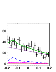
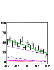
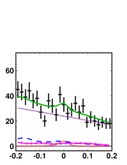
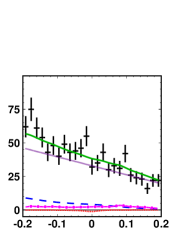
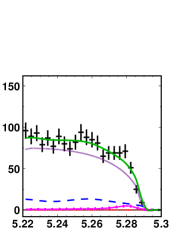
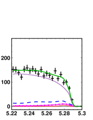
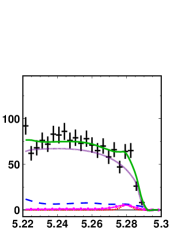
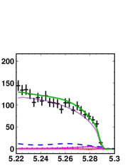
Figure 1: $\Delta E$ (upper) and $M_{\mbox{\scriptsize bc}}$ (lower) distributions for (from left to right) $B^{0}\to\eta^{\prime}\rho^{0}$, $B^{+}\to\eta^{\prime}\rho^{+}$, $B^{0}\to\eta^{\prime}K^{*0}$ and $B^{+}\to\eta^{\prime}K^{*+}$.

+   data       —– combined       - - - - signal       $\cdot\!\!\cdot\!\!\cdot\!\!\cdot\!\!\cdot\!\!\cdot\!\!\cdot\!\cdot$ udsc       – – – $B\bar{B}$       -$\cdot$-$\cdot$ rare B

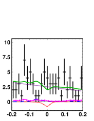
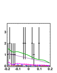
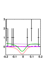
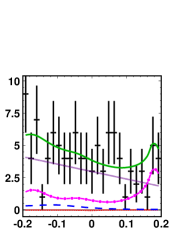
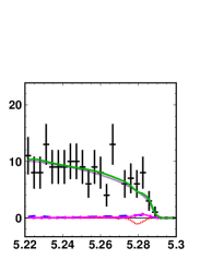
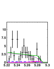
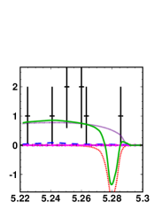
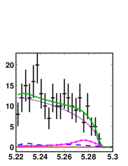
Figure 2: $\Delta E$ (upper) and $M_{\mbox{\scriptsize bc}}$ (lower) distributions for (from left to right) $B^{0}\to\eta^{\prime}\phi$, $B^{0}\to\eta^{\prime}\eta$, $B^{0}\to\eta^{\prime}\eta^{\prime}$ and $B^{0}\to\eta^{\prime}\omega$.

Figure 3: Distributions of likelihood vs. branching fraction for each decay. The systematic error is included as described in the text. Two dashed lines indicate ${\mathcal{B}}=0$ and the 90% confidence level upper limit.

VI Systematics

Systematic errors on the branching fractions are estimated with various high statistics data samples. The dominant sources are the uncertainties in the reconstruction efficiency of charged tracks (3–4%), the uncertainties in the reconstruction efficiencies of $\eta$ mesons, $\pi^{0}$’s and photons (3–6%) and the $K_{S}^{0}$ reconstruction efficiency uncertainty (4%). Other systematic uncertainties arise from signal MC statistics (2%), likelihood ratio selections (2%), uncertainties of the subdecay branching fractions as given by the PDG (1.7–3.0%), the number of $B\bar{B}$ mesons produced (1.4%) and the uncertainty from particle identification (0.5–1.3%). In addition, we calculate systematic uncertainties for the fitting procedure by varying all PDF shape parameters by $\pm 1\sigma$. Background normalization systematic uncertainties are estimated by varying the background normalizations by 20%-50% while those for $\Delta E$/$M_{\mbox{\scriptsize bc}}$ corrections are obtained by varying the corrections by one standard deviation. Since for most decays the fits yield branching fractions close to zero, we use absolute errors in these cases. Fractional errors are translated into absolute values by multiplying the obtained upper limit value by the fractional error. The combined absolute errors are decay dependent and lie in the range (0.01 – 4.93 )$\times 10^{-6}$. The total systematic uncertainties are listed in Table 6.

Table 6: Total systematic uncertainties for each decay. Listed are combined errors for fitting, efficiency related errors and the error in the number of $B\bar{B}$ events. Conservatively, we take the total systematic error to be the linear sum of these. All errors are in absolute values in units of $10^{-7}$.

Decay	Fitting	Efficiency	#$B\bar{B}$	Total
$B^{0}\to\eta^{\prime}\rho^{0}$	${}^{+0.33}_{-1.76}$	$0.07$	$0.02$	${}^{+0.42}_{-1.85}$
$B^{+}\to\eta^{\prime}\rho^{+}$	${}^{+2.90}_{-5.53}$	$0.32$	$0.06$	${}^{+3.28}_{-5.91}$
$B^{0}\to\eta^{\prime}K^{*0}$	${}^{+0.04}_{-0.03}$	$0.16$	$0.04$	${}^{+0.24}_{-0.23}$
$B^{+}\to\eta^{\prime}K^{*+}$	${}^{+0.84}_{-10.10}$	$0.21$	$0.04$	${}^{+1.09}_{-10.35}$
$B^{0}\to\eta^{\prime}\phi$	$\pm 0.10$	$0.03$	$0.01$	$\pm 0.14$
$B^{0}\to\eta^{\prime}\eta$	${}^{+2.43}_{-0.36}$	$0.26$	$0.05$	${}^{+2.74}_{-0.67}$
$B^{0}\to\eta^{\prime}\eta^{\prime}$	${}^{+24.85}_{-48.94}$	$0.29$	$0.05$	${}^{+25.19}_{-49.28}$
$B^{0}\to\eta^{\prime}\omega$	${}^{+0.58}_{-5.19}$	$0.16$	$0.03$	${}^{+0.77}_{-5.38}$

VII Upper limit calculation

Since no decay has more than $2\sigma$ significance bib:sigma , we calculate upper limits on the branching fractions by integrating the likelihood function starting at ${\mathcal{B}}=0$ using a Bayesian approach assuming a uniform distribution for ${\mathcal{B}}>0$. We set the upper limit when the integral reaches 90% of the total area under the likelihood function. The systematic error is accounted for by folding the systematic error into the width of the likelihood distribution (Eq. 1) when integrating the likelihood. Thus the upper limit (UL) is calculated with the formula:

$$\frac{\int_{{\mathcal{B}}=0}^{UL}{L_{\text{sys}}(N_{S},N_{B_{j}})d{\mathcal{B}}}}{\int_{{\mathcal{B}}=0}^{1}{L_{\text{sys}}(N_{S},N_{B_{j}})d{\mathcal{B}}}}=0.9,$$ (2)

where $L_{\text{sys}}(N_{S},N_{B_{j}})$ is the likelihood function with its width increased by the systematic error. The likelihood distribution is shown in Fig. 3 for each decay mode.

The thus calculated upper limits are $0.5\times 10^{-6}$ for $B^{0}\to\eta^{\prime}\phi$, $1.3\times 10^{-6}$ for $B^{0}\to\eta^{\prime}\rho^{0}$, and in the range $2.2$–$6.5\times 10^{-6}$ for other modes, as given in Tables 4 and 5. We note that our upper limits for $B^{0}\to\eta^{\prime}K^{*0}$ and $B^{+}\to\eta^{\prime}K^{*+}$ are below the central values of the BaBar measurement.

VIII Summary

In summary, no signal was observed with more than $2\sigma$ significance and stringent upper limits in the range $(0.5$ – $6.5)\times 10^{-6}$ for the decays $B\to\eta^{\prime}\rho$, $B\to\eta^{\prime}K^{*}$, $B^{0}\to\eta^{\prime}\phi$, $B^{0}\to\eta^{\prime}\eta^{(\prime)}$and $B^{0}\to\eta^{\prime}\omega$ have been given. All limits except $B^{0}\to\eta^{\prime}\eta$ are the most stringent upper limits presently available. Our upper limits for $B\to\eta^{\prime}K^{*}$ are below BaBar’s central value.

IX Acknowledgments

We thank the KEKB group for the excellent operation of the accelerator, the KEK cryogenics group for the efficient operation of the solenoid, and the KEK computer group and the National Institute of Informatics for valuable computing and Super-SINET network support. We acknowledge support from the Ministry of Education, Culture, Sports, Science, and Technology of Japan and the Japan Society for the Promotion of Science; the Australian Research Council and the Australian Department of Education, Science and Training; the National Science Foundation of China and the Knowledge Innovation Program of the Chinese Academy of Sciences under contract No. 10575109 and IHEP-U-503; the Department of Science and Technology of India; the BK21 program of the Ministry of Education of Korea, the CHEP SRC program and Basic Research program (grant No. R01-2005-000-10089-0) of the Korea Science and Engineering Foundation, and the Pure Basic Research Group program of the Korea Research Foundation; the Polish State Committee for Scientific Research; the Ministry of Science and Technology of the Russian Federation; the Slovenian Research Agency; the Swiss National Science Foundation; the National Science Council and the Ministry of Education of Taiwan; and the U.S. Department of Energy.

References

(1)
B. Aubert et al. (BaBar Collaboration),
Phys. Rev. Lett. 95 (2005) 131803.
(2)
J. Schümann et al. (Belle Collaboration),
Phys. Rev. Lett. 97 (2006) 061802.
(3)
B. Aubert et al. (BaBar Collaboration),
Phys. Rev. Lett. 98 (2007) 051802.
(4)
C. W. Chiang, M. Gronau, J. L. Rosner and D. A. Suprun,
Phys. Rev. D 70 (2004) 034020.
(5)
M. Beneke and M. Neubert,
Nucl. Phys. B 675 (2003) 333.
(6)
H. K. Fu, X. G. He and Y. K. Hsiao,
Phys. Rev. D 69 (2004) 074002.
(7)
B. Aubert et al. (BaBar Collaboration),
Phys. Rev. D 73 (2006) 071102.
(8)
S. Kurokawa and E. Kikutani, Nucl. Instr. and Meth. A 499, (2003) 1,
and other papers included in this volume.
(9)
A. Abashian et al. (Belle Collaboration),
Nucl. Instr. and Meth. A 479 (2002) 117.
(10) Z. Natkaniec et al. (Belle SVD2 Group),
Nucl. Instr. and Meth. A 560, (2006) 1.
(11)
F. Fang, Ph.D thesis, University of Hawaii (2003).
(12)
The Fox-Wolfram moments were introduced in
G. C. Fox and S. Wolfram, Phys. Rev. Lett. 41 (1978) 1581.
The Fisher discriminant used by Belle, based on modified Fox-Wolfram
moments (SFW), is described in
K. Abe et al. (Belle Collaboration), Phys. Rev. Lett. 87,
(2001) 101801; and
K. Abe et al. (Belle Collaboration), Phys. Lett. B 511 (2001) 151.
Here, six of the possible
eight Fox-Wolfram moments were used, however, was later found to be
correlated with for two body decays and therefore is omitted in this
analysis leaving the five SFW moments
, , , and .
(13)
R. A. Fisher, Annals of Eugenics 7 (1936) 179.
(14)
R. Ammar et al., Phys. Rev. Lett. 71 (1993) 674.
(15)
H. Kakuno et al., Nucl. Instr. and Meth. A 533 (2004) 516.
(16)
D. J. Lange, Nucl. Instr. and Meth. A 462 (2001) 152.
(17)
E. Barberio and Z. Wa̧s, Comp. Phys. Comm. 79 (1994) 291.
(18)
J. E. Gaiser et al. (Crystal Ball Collaboration), Phys. Rev. D 34
(1986) 711.
(19)
H. Albrecht et al. (ARGUS Collaboration),
Phys. Lett. B 241 (1990) 278.
(20)
S. Eidelman et al. (Particle Data Group),
Phys. Lett. B 592 (2004) 1.
(21)
The statistical significance of the signal
is calculated as ,
where and denote
the likelihood value at zero branching fraction and the value at one standard
deviation of the systematic error below the maximum
likelihood, respectively.