Charge-Separated Atmospheric Neutrino-Induced Muons in the MINOS Far Detector

Abstract

We found $140$ neutrino-induced muons in $854.24$ live days in the MINOS far detector, which has an acceptance for neutrino-induced muons of $6.91\times 10^{6}\text{cm}^{2}\text{sr}$. We looked for evidence of neutrino disappearance in this data set by computing the ratio of the number of low momentum muons to the sum of the number of high momentum and unknown momentum muons for both data and Monte Carlo expectation in the absence of neutrino oscillations. The ratio of data and Monte Carlo ratios, $\cal{R}$, is

$${\cal R}=0.65^{+0.15}_{-0.12}(\text{stat})\pm 0.09(\text{syst}),$$

a result that is consistent with an oscillation signal. A fit to the data for the oscillation parameters $\sin^{2}2\theta_{23}$ and $\Delta m^{2}_{23}$ excludes the null oscillation hypothesis at the $94$% confidence level. We separated the muons into $\mu^{-}$ and $\mu^{+}$ in both the data and Monte Carlo events and found the ratio of the total number of $\mu^{-}$ to $\mu^{+}$ in both samples. The ratio of those ratios, $\hat{\mathcal{R}}_{CPT}$, is a test of CPT conservation. The result

$$\hat{\mathcal{R}}_{CPT}=0.72^{+0.24}_{-0.18}(\text{stat})^{+0.08}_{-0.04}(\text{syst}),$$

is consistent with CPT conservation.

I Introduction

Measurements of atmospheric neutrinos by Super-Kamiokande experiment have shown that there is a deficit of $\nu_{\mu}$ when compared to expectations Fukuda et al. (1998a, b, c, 1999a, 1999b, 2000); Ashie et al. (2004, 2005); Abe et al. (2006). The hypothesis that best describes this deficit is the oscillation of $\nu_{\mu}(\overline{\nu}_{\mu})\rightarrow\nu_{\tau}(\overline{\nu}_{\tau})$  Yao et al. (2006a); Kayser (2004), with the oscillation probability given by

$$P_{\nu_{\mu}\rightarrow\nu_{\tau}}=\sin^{2}2\theta_{23}\sin^{2}(1.27\Delta m^{2}_{23}L/E),$$ (1)

where $\theta_{23}$ is the mixing angle, $\Delta m^{2}_{23}=|m_{3}^{2}-m_{2}^{2}|$ is the mass squared difference in eV² between the neutrino mass states, $L$ is the distance in km traveled by the neutrino, or its baseline, and $E$ is the energy of the $\nu_{\mu}$ in GeV fin . The Super-Kamiokande data is best fit by the oscillation hypothesis with parameters $(\sin^{2}2\theta_{23},\Delta m^{2}_{23})=(1.0,2.4\times 10^{-3}\,{\rm eV^{2}})$ Ashie et al. (2005); Abe et al. (2006); the ranges for these parameters given by the 90% confidence contours of the zenith angle oscillation fit are $\sin^{2}2\theta_{23}>0.92$ and $1.5<\Delta m^{2}_{23}<3.4\times 10^{-3}\,{\rm eV^{2}}$. The MACRO Ambrosio et al. (2001, 2004) and Soudan 2 Sanchez et al. (2003); Allison et al. (2005) results are consistent with those obtained by Super-Kamiokande. For the MINOS analysis of atmospheric neutrinos with an interaction vertex in the detector, the parameter ranges are $\sin^{2}2\theta_{23}>0.2$ and $7\times 10^{-5}<\Delta m^{2}_{23}<5\times 10^{-2}\,{\rm eV^{2}}$ Adamson et al. (2006a). Below we extend the MINOS atmospheric analysis to neutrino-induced muons observed in the MINOS far detector.

The oscillation hypothesis for the atmospheric neutrino deficit has received strong support from the first results of the MINOS long baseline experiment. MINOS, which sends $\nu_{\mu}$ produced at Fermilab to a detector 735 km away in northern Minnesota Michael et al. (2006a), finds $(\sin^{2}2\theta_{23},\Delta m^{2}_{23})=(1.00,2.74\times 10^{-3}\,{\rm eV^{2}})$ Michael et al. (2006b), when fitting their $\nu_{\mu}$ events; the ranges of these parameters given by the 90% confidence contours are $\sin^{2}2\theta_{23}>0.72$ and $2.2<\Delta m^{2}_{23}<3.8\times 10^{-3}\,{\rm eV^{2}}$. The K2K long baseline experiment, which sent $\nu_{\mu}$ produced at KEK to the Super-Kamiokande detector located 250 km away, also found consistent results – $(1.0,2.8\times 10^{-3}\,{\rm eV^{2}})$ Aliu et al. (2005); Ahn et al. (2006) with 90% confidence ranges for the parameters of $\sin^{2}2\theta_{23}>0.55$ and $1.9<\Delta m^{2}_{23}<3.6\times 10^{-3}\,{\rm eV^{2}}$.

Since the magnetized MINOS far detector distinguishes $\mu^{-}$ from $\mu^{+}$, MINOS data can be used as a probe of CPT conservation in the neutrino sector. CPT conservation requires that the probability of an atmospheric $\nu_{\mu}$ of a given energy remaining a $\nu_{\mu}$ after traveling from its origin to its point of interaction be equal to the probability that an atmospheric $\overline{\nu}_{\mu}$ of the same energy remains a $\overline{\nu}_{\mu}$ after traveling the same distance Kayser (2004). We consequently test CPT conservation by comparing $\nu_{\mu}$-induced $\mu^{-}$ and $\overline{\nu}_{\mu}$-induced $\mu^{+}$ with respect to expectations, as a measure of whether the atmospheric $\nu_{\mu}$ and $\overline{\nu}_{\mu}$ are disappearing at the same rate. Effects induced by charged current interactions of the $\nu_{e}$ components of the neutrino eigenstates with the earth could masquerade as apparent CPT violation. However, distortions from matter effects are estimated to be small for most of the $\theta_{13}$ range compatible with the CHOOZ limit Apollonio et al. (1999). The average induced $\nu_{\mu}/\overline{\nu}_{\mu}$ event rate asymmetry is estimated to be less than 10% Palomares-Ruiz and Petcov (2005). Therefore, at our current level of statistical accuracy we can ignore matter effects and describe $\nu_{\mu}(\overline{\nu}_{\mu})\rightarrow\nu_{\tau}(\overline{\nu}_{\tau})$ oscillations using the two flavor approximation in Eq. (1).

After briefly discussing the detector in §II, we describe our event sample in §III.1 and the Monte Carlo event generation in §III.2. In §III.3, we describe the cuts used in selecting the sample of muons to be analyzed. We present the oscillation analysis in §IV and the probe of CPT conservation using charge separated neutrino-induced $\mu^{-}$ and $\mu^{+}$ in §V.

II The MINOS Far Detector

The MINOS far detector is a steel-scintillator sampling calorimeter located at a depth of 2070 meters-water-equivalent (m.w.e.) in the Soudan mine in northern Minnesota Michael et al. (2006a). The detector is made up of 486 vertical octagonal planes of 2.54 cm thick steel laminates, interleaved with 484 planes of 1 cm thick extruded polystyrene scintillator strips and a 2.5 cm wide air gap. Each scintillator plane has 192 strips of width 4.1 cm. The length of each strip depends on its position in the plane and varies between 3.4 and 8.0 m. The scintillator strips in alternating detector planes are oriented at $\pm 45^{\circ}$ to the vertical. The modular detector consists of two supermodules (SM) separated by a gap of 1.1 m. The detector coordinate system has the y axis pointing up, the z axis along the detector long axis, pointing away from Fermilab and the x axis forms a right-handed coordinate system.

Scintillation light from charged particles traversing the MINOS plastic scintillator is collected with wavelength shifting (WLS) plastic fibers embedded in the scintillator strips. The WLS fibers are coupled to clear optical fibers at both ends of a strip and are read out using 16-pixel multi-anode phototmultiplier tubes (PMTs). The signals from eight strips, separated by approximately 1 m within the same plane, are optically summed, or multiplexed, and read out by a single PMT pixel. The multiplexing pattern is different for the two sides of the detector, enabling the resulting eightfold ambiguity to be resolved for single particles. For all other types of events, ambiguities are resolved effectively using additional information from timing and event topology.

To measure the momentum of muons traversing the detector, the steel has been magnetized into a toroidal field configuration using a current-carrying coil that runs through the central axis of each SM. A finite element analysis calculation shows that each SM is magnetized to an average value of $\sim 1.3$ T by the 15 kA current loop. The field is saturated near the coil hole at a strength of approximately 1.8 T, falling to about 1 T near the edges. Further details about the MINOS detector can be found in Michael et al. (2006a).

To distinguish upward-going neutrino-induced muons from the downward cosmic ray background requires excellent timing resolution. The MINOS timing system has a least count of 1.56 ns. However, the timing resolution is dominated by the 8 ns fluorescence decay time in the WLS fiber Border et al. (2001). The overall resolution is determined by the convolution of the least count with the fluctuations in the arrival times of the photons at the PMT. We calibrated the timing system by measuring the time offsets between each channel. For this determination Rebel (2004); Blake (2005), we selected a sample of downward through-going cosmic ray muons with well-reconstructed tracks. For each hit along a track we measured the travel times from the track entrance point in the detector to the hit location and corrected those values for both the rise time of the signal and the propagation of light along the fibers. We then compared these times with the time expected for a relativistic muon traversing the same distance and computed the offset between the measured and expected times for each hit, $\Delta t$. The timing calibration constants are obtained using an iterative method to minimize the mean $\Delta t$ for each channel. After calibration, linear timing fits are again applied to the times and positions of the hits on each muon track. The r.m.s. deviation between the measured and fitted times is calculated for each track. Figure 1 shows the distribution of these r.m.s. deviations. In this figure, the distribution has been fit to a Gaussian with a mean of $2.31\pm 0.03$ ns, a value that represents the overall timing resolution of the detector.

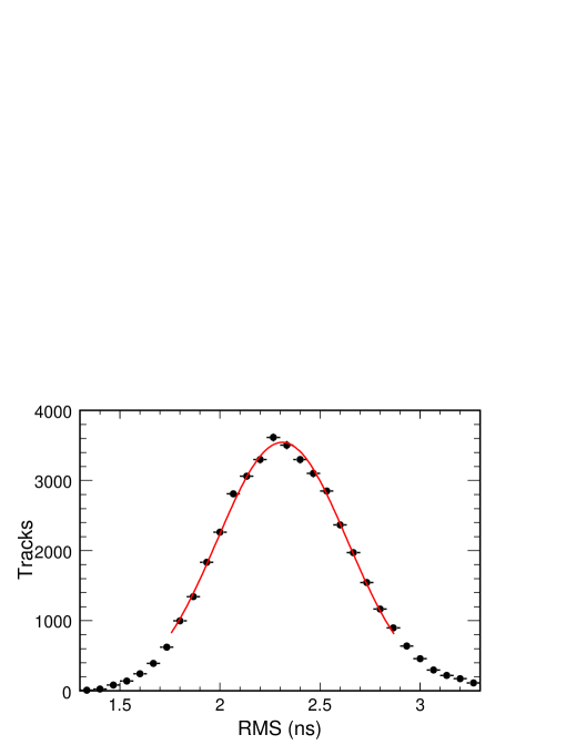
Figure 1: Distribution of the r.m.s. deviations of the measured hit times from the calculated hit times for calibration tracks. The resolution of the system is the mean of a Gaussian fit to the distribution, $2.31\pm 0.03$ ns.

III Data Analysis

In the analyses presented here we use neutrino-induced muons, which are defined as events that come from below or slightly above the horizon. These events are essentially uncontaminated by the background of downward-going atmospheric muons. We analyze two types of events: those that pass completely through the detector (“through-going muons”) and those that enter and stop in the detector (“stopping muons”). Earlier MINOS results for events with an interaction vertex in the detector (“contained events”) appear in Adamson et al. (2006a). We distinguish between neutrino-induced muons with well-determined momenta and neutrino-induced muons whose charge and momentum are undetermined (c.f., §III.4).

III.1 Data Sample

The data presented here represent $854.24$ live days and were taken between August 1, 2003 and April 30, 2006. The geometric acceptance of the detector for neutrino-induced muons is $6.91\times 10^{6}\text{cm}^{2}\text{sr}$. We found a total of $140$ neutrino-induced muons in this data set.

III.2 Simulated Muons

III.2.1 Atmospheric Neutrino-induced Muons

We generated a large sample of simulated neutrino-induced muons in the MINOS far detector using the Bartol 96 Agrawal et al. (1996) neutrino flux tables along with the default Nuance neutrino interaction model Casper (2002) and the Grv94 Gluck et al. (1995) parton distribution functions. We first simulated neutrino-induced muons passing through the surface of a box surrounding the MINOS far detector and then propagated these muons through the detector with the MINOS Geant-based detector Monte Carlo simulation. A total of $6.5\times 10^{5}$ neutrino-induced muon events, the equivalent of 2500 years of live time, were generated in this way. The momentum distributions simulated for the neutrino-induced $\mu^{-}$ and $\mu^{+}$ in MINOS are shown in Fig. 2 for neutrinos without oscillations and for neutrinos with an oscillation signal using the Super-Kamiokande parameters Ashie et al. (2005). This figure shows that the oscillation signal affects mostly muons with low momenta.

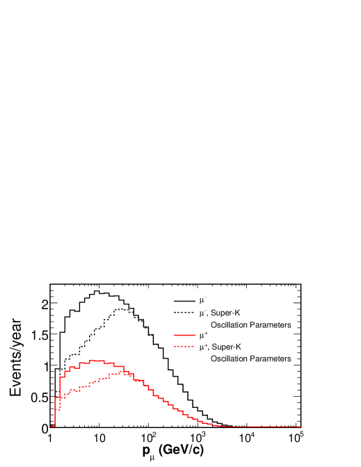
Figure 2: Input momentum distribution for neutrino-induced $\mu^{-}$ and $\mu^{+}$ calculated with the Nuance simulation package. The distributions in the MINOS Far detector without oscillations and with the Super-Kamiokande determined values of $\sin^{2}2\theta_{23}$ and $\Delta m^{2}_{23}$ are shown. The oscillation affects mostly muons with low momenta.

III.2.2 Cosmic Ray Muons

We simulated each cosmic ray muon event by first choosing its arrival direction from a distribution uniform in solid angle and then associating this direction with the overburden found in the Soudan 2 slant depth map Kasahara (1997). The surface energy of the muon was selected from the known distribution Yao et al. (2006b). Once the surface energy and overburden were chosen, we tested the muon to see whether it survived energy loss processes between the surface and the detector Yao et al. (2006b). We placed the muons that survived on an imaginary box surrounding the detector Hawthorne (1997) and then propagated them though the detector with the MINOS GEANT-based detector simulation.

III.3 Event Selection

All data and simulated muons were analyzed using the standard MINOS reconstruction algorithms and a uniform set of event selection cuts. The selection cuts summarized below are described in further detail in Rebel (2004).

III.3.1 Muon Selection Cuts

We first selected muon events using criteria developed for the study of cosmic ray muons with the MINOS far detector Adamson et al. (2006b). The first two cuts require that there was a track successfully reconstructed in the event (“No Track” cut), and that there is only a single track found by the track-fitting algorithm (“Multiples” cut). The next set of cuts exclude random collections of hits that could be mistaken for muon tracks. These cuts require that: the track must cross at least 20 planes in the detector (“20 Plane” cut); the track must have a pathlength of at least 2 m (“2.0 m Length” cut); the earliest recorded hit of the track be no more than 15 cm from the front or back surface of the detector or 30 cm from any of the remaining surfaces (“Fiducial” cut); and the track fit must have a $\chi^{2}$ per number of degrees of freedom, $\chi^{2}_{fit}/ndf<1.5$.

The next selection cuts were designed to remove events with poor timing information. To ensure the presence of sufficient timing information in the events, we first excluded tracks if fewer than half of the hits come from strips with signals on both ends (“Double-ended Strip Cut”). We determined the direction of the track by plotting the time difference $\Delta T$ (ns) of each hit along the track as a function of its distance $\Delta S$ (m) from the first hit. If the $\it y$ positions of the hits increase along the length of the track, $\Delta S$ is positive; for $\it y$ decreasing along the track, $\Delta S$ is negative. The slope of the linear fit to the $\Delta T/\Delta S$ distribution is $1/\beta=c/v$. The top panel of Fig. 3 shows the $\Delta T/\Delta S$ distribution with the linear fit superposed for a typical cosmic muon; the bottom panel displays the $(x,y)$ positions of the hits in the detector for this muon.

In Fig. 4 we show the distributions of $\chi_{1/\beta}^{2}/ndf$ values for the linear fits to $1/\beta$ for both data and cosmic ray muon Monte Carlo events passing the above cuts. The distribution does not peak at 1 as might be expected for a $\chi^{2}/ndf$ statistic. However, that is unimportant to the analysis since we are using the $\chi_{1/\beta}^{2}/ndf$ value only to define a cut. We defined a cut that requires $\chi_{1/\beta}^{2}/ndf<3.0$ for an event (“$\chi_{1/\beta}^{2}/ndf<3.0$” cut). The cut was selected at the value of $\chi_{1/\beta}^{2}/ndf$ where the number of events falls to $\sim$1% of the peak. This cut maximizes the number of selected events while excluding those events with the worst $\chi_{1/\beta}^{2}/ndf$ values. Although the data and Monte Carlo simulation deviate at low values of $\chi_{1/\beta}^{2}/ndf$ the agreement is excellent near the peak and the cut value. Therefore, the Monte Carlo sample can be used to effectively study the systematic uncertainty introduced into the analysis by this cut.

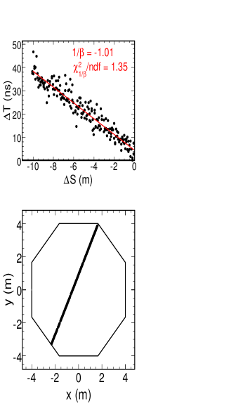
Figure 3: A typical cosmic ray muon in the MINOS far detector. The top panel shows the timing information for the hits along the track with a straight line fit superposed. The legend gives $\Delta T/\Delta S=1/\beta$ and the $\chi^{2}_{1/\beta}/ndf$ of the fit for this muon. The bottom panel shows the $(x,y)$ hit positions of this track. The resolution of the positions is the 4 cm width of the strips.

In the last step of the muon selection, we separated the downward-going from upward-going events. Upward-going events have a positive slope for the straight line fit to the $\Delta T/\Delta S$ distribution. The final muon cut is a check on the up/down separation. The entrance point of a track, and therefore its incoming direction, is determined by the slope of the times of the hits in the detector as a function of their z position. For a few short tracks this information is sufficiently ambiguous that the entrance point can be confused with the exit point of the track causing the reconstruction to interchange the two. As a result, downward-going muons are incorrectly reconstructed as upward-going. We remove these failures by checking the times of the hits in the reconstructed track as a function of their $\it y$ position. The slope of the line fit to the hits as a function of their $\it y$ positions must agree with the reconstructed incoming direction of the track (“Directionality” cut).

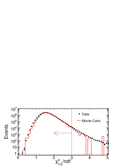
Figure 4: Distribution of $\chi^{2}_{1/\beta}/ndf$ values from the $1/\beta$ determinations for data and cosmic ray muon Monte Carlo events. In this figure, the Monte Carlo distribution has been normalized to the same area as the data distribution. Events with $\chi^{2}_{1/\beta}/ndf<3$ are used in the analysis.

Table 1: Effect of cuts on data and simulated samples. The fraction of the total events remaining is shown. $N$ gives the total number of events in each sample.

Cut	Data	$\mu$ MC	$\nu$-induced MC
	$N=$	$N=$	$N=$
	$3.81\times 10^{7}$	$1.20\times 10^{6}$	$6.47\times 10^{5}$
No Cuts	1.000	–	1.000
No Track	0.800	–	0.862
Multiples	0.743	–	0.848
20 Plane	0.561	0.561	0.606
2.0 m Length	0.557	0.557	0.578
Fiducial	0.534	0.538	0.559
$\chi^{2}_{fit}/ndf<1.5$	0.429	0.447	0.497
Double-ended Strips	0.429	0.447	0.497
$\chi^{2}_{1/\beta}/ndf<3.0$	0.428	0.447	0.497
Directionality	0.428	0.447	0.478

Table 1 shows the effect of the cuts on the data and the two Monte Carlo distributions. We normalize the cosmic ray muon Monte Carlo distributions to the data value at the 20 Plane cut because the Monte Carlo simulation does not account for multiple muon events which make up $\sim 5\%$ of downward-going cosmic ray muons Gaisser (1990). After cuts the selected events consist of muon tracks whose directionality is well determined. The distribution of $1/\beta$ values for the selected muon events is shown in Fig. 5. Since the sample includes both downward-going and upward-going muons and these muons are relativistic, there are two peaks in the $1/\beta$ distribution. The peak at $1/\beta=-1$ are downward-going muons and the peak at $1/\beta=1$ are upward-going muons. Integrating the events in the two peaks shows that the fraction of (upward-going muons)/(downward-going muons) $\sim 10^{-5}$.

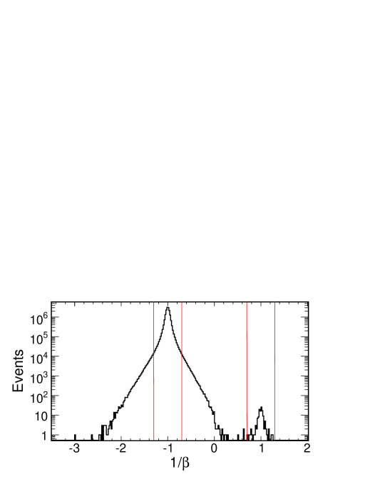
Figure 5: Distribution of $1/\beta$ for upward-going neutrino-induced muons, with a peak at 1, and downward-going cosmic ray muons, with a peak at -1. The vertical lines at 0.7 and 1.3 bracket the events included in the upward-going muon sample.

III.3.2 Upward-Going Neutrino-Induced Muons

As in previous experiments Fukuda et al. (1999a); Allison et al. (2005), we identify upward-going muons that enter the detector as neutrino-induced muons. Events in the range $0.7<1/\beta<1.3$ are included in our neutrino-induced muon data set. The cut was determined using downward-going cosmic ray muons. It was set as the $1/\beta$ range that includes 99% of the events and which is centered on the peak. In the left panel of Fig. 6 we show a well-characterized upward-going muon event. The right panel shows an event excluded by the $1/\beta$ cut.

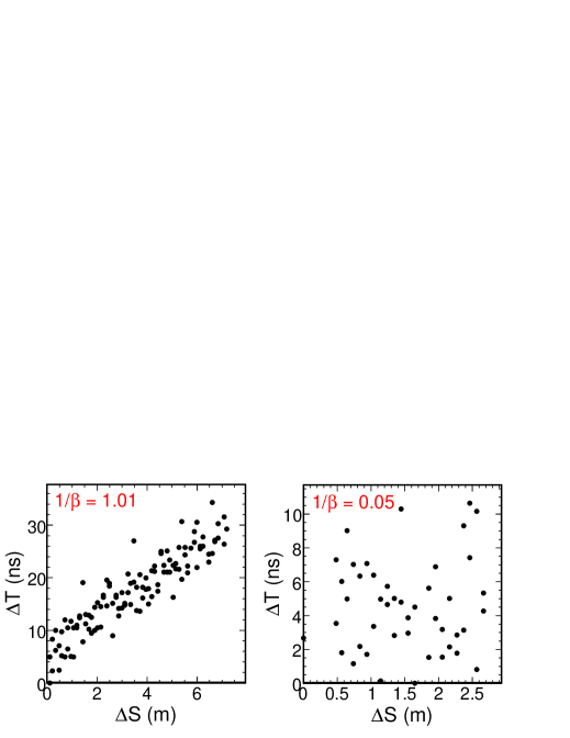
Figure 6: Distributions of $\Delta T/\Delta S$ as in Fig. 3. The left panels shows a typical upward-going muon and the right panel shows a muon excluded by the $1/\beta$ cut from the upward-going sample.

Table 2 shows that our data sample includes $130$ upward-going, neutrino-induced muons in the range $0.7<1/\beta<1.3$. In this table we also show the background from contained vertex interactions where the neutrino interacts close to the detector edge and cannot be separated from muons entering the detector. This background was estimated by calculating the rate of Monte Carlo atmospheric neutrino events that interact inside the detector volume Adamson et al. (2006a). The background includes events that pass the cuts in Table 1 and satisfy the upward-going selection cut. The Monte Carlo events were assumed to oscillate with the best-fit oscillation parameters from Super-Kamiokande Ashie et al. (2005). The 20 Plane cut has been shown to be effective at removing the background due to upward-going pions produced by downward-going cosmic ray muons interacting in the rock surrounding the detector.

III.3.3 Horizontal Muons

In this analysis, we also include muons coming from along and slightly above the detector’s horizon. The flat overburden of the Soudan site Kasahara (1997) makes this search feasible. The slant depth of rock between the detector and the surface for incoming directions above the horizon increases approximately as $\sec\theta$, where $\theta$ is the zenith angle. Only the highest energy cosmic ray muons ($E_{\mu}>100$ TeV) have sufficient energy to penetrate the large column of rock present for muons coming from directions near the horizon. Since the intensity of cosmic ray muons falls as $E^{-2.7}$, very few cosmic ray muons survive to reach the detector, implying that muons from near the detector’s horizon are neutrino-induced. These events are important to the analysis because they sample neutrino-induced muons with lower values of $L/E$ than the upward-going muons. Eq. (1) shows that the average oscillation probability for these horizontal muons is lower than for upward-going neutrino-induced muons and they add information important in determining the neutrino flux normalization, a parameter used in the oscillation analysis in §IV.3.

We require that the measured velocity of the downward-going muons be in the range $-1.3<1/\beta<-0.7$ . To determine the maximum angle above the horizon from which we can distinguish horizontal muons from cosmic ray muons, we use the zenith angle distribution for all events shown in Fig. 7. The distribution is steeply falling for $\cos\theta<0.25$ but becomes approximately constant for $\cos\theta<0.1$. The rate of neutrino-induced muons is expected to be approximately independent of $\cos\theta$ Yao et al. (2006b). We select events with $\cos\theta<0.05$ to minimize the background from cosmic ray muons. To estimate this background we fit an exponential to the distribution of Fig. 7 for $0.1\leq\cos\theta\leq 0.2$, a similar procedure to that used by Super-Kamiokande Fukuda et al. (1999a). The exponential fit is shown in the figure; it has the form $y=\exp(a+b\cos\theta)$, where $a=-3.59$ and $b=51.65$. Fig. 7 shows that the background at $\cos\theta=0.05$ is 0.3 events and is negligible for smaller values of $\cos\theta$.

In Table 2 we show that there are $10$ horizontal, neutrino-induced muons in the data sample. The background shown includes both cosmic ray downward-going muons and the contained vertex events discussed previously.

Table 2: Observed upward-going and horizontal muons. The background accounts for both contained vertex neutrino interactions and downward-going cosmic ray muons.

Muon Type	Events	Background
		Contained	Cosmic $\mu$
Upward-going	$130$	4.2	0.0
Horizontal	$10$	0.1	0.3

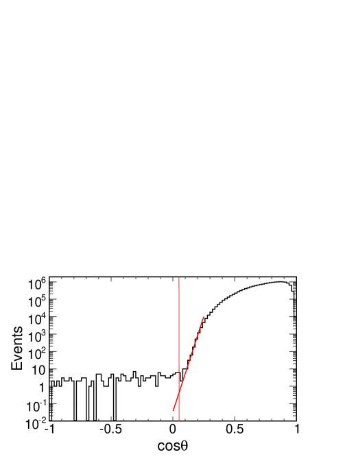
Figure 7: The $\cos\theta$ distribution for all incoming muons. The data are fit to an exponential between $0.1\leq\cos\theta\leq 0.2$ to estimate the background of cosmic ray muons in the horizontal neutrino-induced muon signal region. The fit is shown in the figure. As indicated, we select muons coming from directions with $\cos\theta<0.05$.

III.4 Charge Sign and Momentum Determination

Previous oscillation analyses based on neutrino-induced muons have typically divided the event sample into through-going and stopping muons. The experiments that presented these analyses could only measure the muon momentum directly for stopping muons. Since the MINOS far detector is magnetized, we can measure the muon momentum and charge sign for both types of neutrino-induced muons.

To determine whether the charge and momentum of a neutrino-induced muon has been determined accurately, we have developed a criterion based on the measured curvature of the muon track. We first draw a straight line between the end points on the track and then use the deviations of the remaining track points from the line to form a $\chi^{2}$ statistic, $\chi^{2}_{\text{line}}/ndf$. Large values of $\chi^{2}_{\text{line}}/ndf$ indicate significant bending in the magnetic field which leads to a good determination of the charge sign and momentum.

We use our Monte Carlo simulation to set the value of $\chi^{2}_{\text{line}}/ndf$ that selects neutrino-induced muons with good momentum and charge sign determination. As a test of whether the $\chi^{2}_{\text{line}}/ndf$ values are well simulated we compare in Fig. 8 the distributions of $\chi^{2}_{\text{line}}/ndf$ for stopping muons in the cosmic ray data, in the cosmic ray muon Monte Carlo simulation, and in the neutrino-induced muon Monte Carlo simulation. The Monte Carlo distributions have been normalized to have the same number of events as in the data. Fig. 8 shows that the cosmic ray muon Monte Carlo simulation provides a high statistics match to the cosmic ray data. Since the stopping cosmic ray muons have energies $<20$ GeV, the maximum energy of a normally incident stopping muon, these low energy cosmic events provide a sample of muons with a distribution in energy similar to neutrino-induced muons. Also superposed on these distributions is that of the Monte Carlo neutrino-induced muons. This figure suggests that the neutrino-induced Monte Carlo simulation can be used to determine an appropriate value of $\chi^{2}_{\text{line}}/ndf$ for selecting events with good charge sign and momentum determination.

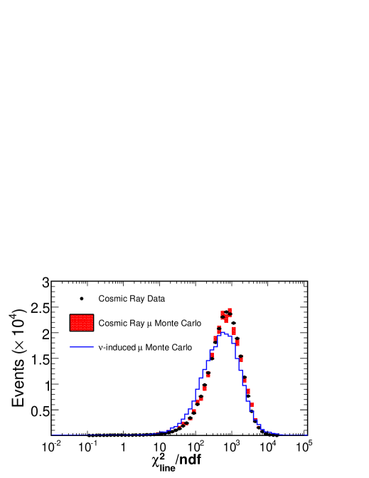
Figure 8: Comparison of the $\chi^{2}_{\text{line}}/ndf$ distributions for stopping muons in the cosmic ray data (points), in the cosmic ray Monte Carlo simulation (boxes), and in the neutrino-induced Monte Carlo simulation (line). The vertical extent of the boxes representing the cosmic ray Monte Carlo simulation indicate the statistical uncertainty for the points.

In Fig. 9 we show the fraction of Monte Carlo neutrino-induced muons with correct charge identification, or purity, as a function of $\chi^{2}_{\text{line}}/ndf$. The purity is approximately 97% at $\chi^{2}_{\text{line}}/ndf=10$ and rises to over 99% with increasing values of $\chi^{2}_{\text{line}}/ndf$. We identify muons with $\chi^{2}_{\text{line}}/ndf>10$ as having good charge-sign and momentum determination; muons with $\chi^{2}_{\text{line}}/ndf<10$ are assumed to have poor charge-sign and momentum determination.

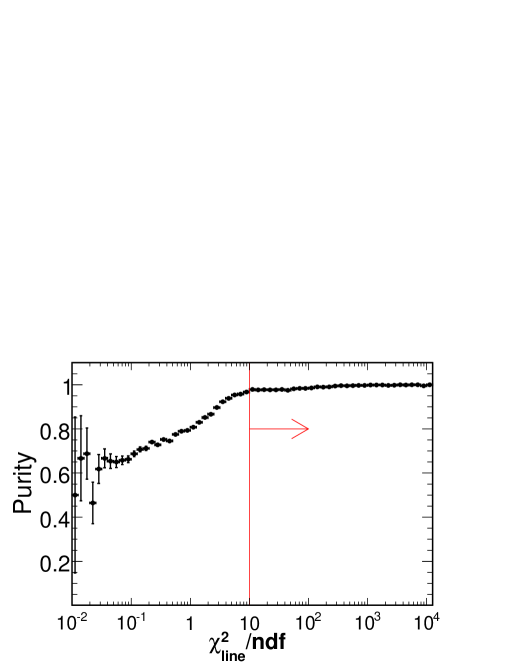
Figure 9: Purity of the charge sign determination for neutrino-induced muons as a function of $\chi^{2}_{\text{line}}/ndf$. Events with $\chi^{2}_{\text{line}}/ndf>10$ have well-determined charge sign and momentum.

We further divided the Monte Carlo muons with $\chi^{2}_{\text{line}}/ndf>10$ into two samples based on their momentum, a separation that roughly distinguishes muons whose parent neutrinos have a relatively large probability of oscillation from those with a lower probability. The ‘low momentum’ (L) sample includes muons with fit momentum, $p_{fit}$, in the range $1\leq p_{fit}<10$ GeV/$c$. The ‘high momentum’ (H) sample includes muons in the range $10\leq p_{fit}<100$ GeV/$c$. No muons with $\chi^{2}_{\text{line}}/ndf>10$ have $p_{fit}>100$ GeV/$c$. The muons with $\chi^{2}_{\text{line}}/ndf<10$ are in the ’unknown momentum’ (U) sample.

The quality of the momentum determination can be deduced from the Monte Carlo simulation using the r.m.s. momentum resolution, $(\Delta p/p)=\sqrt{\langle(p_{truth}-p_{fit})^{2}/p_{truth}^{2}\rangle}$, where $p_{truth}$ is the known momentum of the muons. In Fig. 10 we show $\Delta p/p$, as a function of $\chi^{2}_{\text{line}}/ndf$ for the low momentum and high momentum samples. The low momentum Monte Carlo muons have a momentum resolution of less than 50% at $\chi^{2}_{\text{line}}/ndf=10$ and the resolution decreases to 10% with increasing values of $\chi^{2}_{\text{line}}/ndf$. For the high momentum muons the momentum resolution is less than 30% at $\chi^{2}_{\text{line}}/ndf=10$ and it decreases to 10% as $\chi^{2}_{\text{line}}/ndf$ increases.

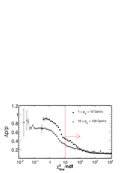
Figure 10: Momentum resolution for Monte Carlo neutrino-induced muons as a function of $\chi^{2}_{\text{line}}/ndf$. The line at $\chi^{2}_{\text{line}}/ndf=10$ shows the cut used in the analyses.

Fig. 11 shows the distributions of parent neutrino energies for the low momentum, high momentum, and unknown momentum muons as determined by the Monte Carlo simulation. The neutrinos producing low momentum muons have energies that peak near 10 GeV. The high momentum muons are produced by neutrinos with energies that peak near 50 GeV. The unknown momentum muons are produced by even higher energy neutrinos, with a peak energy near 250 GeV. Comparing the peak energies of the various neutrino distributions we see from Eq. (1) that the low momentum muons are those that are expected to show the strongest oscillation signal, a result also seen in Fig. 2

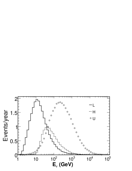
Figure 11: Distribution of energies for neutrinos producing neutrino-induced muons observed in the MINOS detector as determined by the Monte Carlo simulation. The neutrinos producing low momentum muons are shown by the solid line, those producing high momentum muons are shown by the dashed line and those producing unknown momentum muons are shown by open circles. Neutrinos producing muons detected by MINOS have energies $\gtrsim 2$ GeV.

In Fig. 12 we show the distributions of $\chi^{2}_{\text{line}}/ndf$ for the selected neutrino-induced muons from the data and unoscillated Monte Carlo simulation normalized by live time. The muons with $\chi^{2}_{\text{line}}/ndf<10$ are from high energy neutrinos and are not expected to show a strong oscillation signal. Those muons with $\chi^{2}_{\text{line}}/ndf>10$ are from lower energy neutrinos, a sample expected to show an oscillation signal.

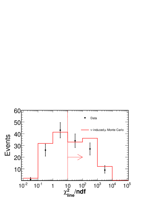
Figure 12: Comparison of the $\chi^{2}_{\text{line}}/ndf$ distributions for neutrino-induced muon data and unoscillated Monte Carlo simulation.

The results of applying the $\chi^{2}_{\text{line}}/ndf$ cut to the sample of $140$ neutrino-induced muons are given in Table 3. In this table, the events with $\chi^{2}_{\text{line}}/ndf>10$ have been further separated by charge identification and momentum. The calculated background contribution is shown as well as the Monte Carlo expectation in the absence of oscillations. Figure 13 shows the fit momentum distributions for data and unoscillated Monte Carlo simulation using the combined low momentum and high momentum muon samples. The unknown momentum muons are not included in this figure. The first bin in Fig. 13 shows a deficit of events in the data relative to Monte Carlo expectation without oscillations (c.f., Fig. 2).

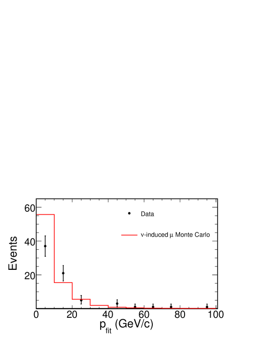
Figure 13: Distribution of fit momenta for events in the combined low momentum and high momentum data samples. The Monte Carlo expectation for no oscillations is shown by the solid line. The unknown momentum muons are not included in this figure.

Table 3: Momentum and charge sign of selected neutrino-induced muons. The calculated background is shown as well as the Monte Carlo expectation in the absence of oscillations.

$p_{fit}$ (GeV)	Data	Bkgd	MC
	$\mu^{-}$
$1-10$     (L)	21	2.2	37.5
$10-100$  (H)	20	0.2	17.5
	$\mu^{+}$
$1-10$     (L)	16	1.3	19.3
$10-100$  (H)	13	0.2	8.6
	U
unknown (U)	70	0.7	76.5

IV Oscillation Analysis

After first discussing the systematic uncertainties associated with the analysis procedure, we test the neutrino-induced muons in Table 3 for evidence of neutrino oscillations.

IV.1 Systematic Uncertainties

There are several sources of systematic uncertainty in this analysis. These are due to both the event reconstruction and the physics modeling. These uncertainties are summarized in Table 4.

The sources of reconstruction systematic uncertainties are those associated with the data selection cuts (1) $\chi^{2}_{fit}/ndf$, (2) $\chi^{2}_{1/\beta}/ndf$ and (3) $\chi^{2}_{\text{line}}/ndf$, where the numbers refer to Table 4. The systematic uncertainties for these cuts were all computed in a similar manner. For example, we computed the systematic uncertainty on $\chi^{2}_{1/\beta}/ndf$ by establishing that the cut value of $\chi^{2}_{1/\beta}/ndf=3$ selects 98.9% of events seen in Fig. 4. We divided the total Monte Carlo data set into 12 subsamples of 20,000 events each. For each subsample we found the value of $\chi^{2}_{1/\beta}/ndf$ that accepts 98.9% of the events. The variance in these values of $\chi^{2}_{1/\beta}/ndf$ divided by the nominal value of the $\chi^{2}_{1/\beta}/ndf$ cut is the $1\sigma$ uncertainty given in Table 4. The $1\sigma$ values for the uncertainties in $\chi^{2}_{fit}/ndf$ and $\chi^{2}_{\text{line}}/ndf$ were computed in a similar manner.

The first source of systematic uncertainty in the physics modeling is the (4) overall normalization of the calculated neutrino flux. Uncertainties in the primary cosmic ray fluxes and the hadronic production are the main contributors to the overall uncertainty in the normalization. Combining these sources gives an uncertainty in the flux normalization of 15% Barr et al. (2006). There are three sources of systematic uncertainty in the ratio of the number of muons induced by low energy neutrinos to those induced by high energy neutrinos. One contribution comes from (5) the uncertainty in the spectral index of the atmospheric neutrino energy spectrum. The neutrino flux is proportional to $E_{\nu}^{-(\gamma+1)}$, with the value of the spectral index, $\gamma=1.7\pm 0.05$ Gaisser (1990), a 3% uncertainty in the spectral index. In addition, the uncertainties in the neutrino and anti-neutrino cross sections contribute another 7% Auchincloss et al. (1990) to the rate of muons coming from neutrinos with energies $<30$ GeV (6) and 2% Yao et al. (2006a) for muons coming from neutrinos with energies $>30$ GeV (7).

Table 4: Sources of systematic uncertainty in low to high momentum event ratio ${\cal R}$.

Source	$\sigma$	$\Delta\mathcal{R}_{k}$
Reconstruction systematics:
(1) $\chi^{2}_{fit}/ndf<1.5$	0.01	$<5\times 10^{-4}$
(2) $\chi^{2}_{1/\beta}/ndf<3.0$	0.01	$<1\times 10^{-4}$
(3) $\chi^{2}_{\text{line}}/ndf<10$	0.27	0.02
Model systematics:
(4) Normalization	0.15	$<1\times 10^{-4}$
(5) Spectral Index	0.03	0.08
(6) Cross Section ($E<30$ GeV)	0.07	0.03
(7) Cross Section ($E>30$ GeV)	0.02	0.01
$\Delta{\cal R}=\sqrt{\sum(\Delta\mathcal{R}_{k})^{2}}$		0.09

IV.2 Low to High and Unknown Momentum Event Ratio

One way to look for evidence of neutrino oscillations in the neutrino-induced muons is to take the ratio of the number of low momentum muons, which are more likely to show an oscillation signal, to the sum of the number of high momentum and unknown momentum muons, which are less likely, and compare this ratio with its Monte Carlo expectation including backgrounds. In the data, this ratio of low to the sum of high and unknown momentum muons is given by

$$R_{{L}/{H+U}}^{data}=\sum_{L}(N_{\mu^{-}}+N_{\mu^{+}}){\Large/}\sum_{H+U}(N_{\mu^{-}}+N_{\mu^{+}}),$$ (2)

where $N_{\mu^{-}}$ is the number of $\mu^{-}$ observed in a bin and $N_{\mu^{+}}$ is the number of $\mu^{+}$ observed in a bin. The sum over $L$ includes events in the range $1<p_{fit}<10$ GeV/$c$, and the sum over $(H+U)$ includes the remaining high momentum and unknown momentum events. In the Monte Carlo simulation, a similar ratio, $R_{{L}/{H+U}}^{MC}$, is defined. In the absence of oscillations, the ratio of these two quantities, $\mathcal{R}$, will be consistent with unity; if an oscillation signal is present, $\mathcal{R}$ will be less than unity.

We computed the systematic uncertainty in this ratio with our Monte Carlo simulation by varying the value of each of the parameters in Table 4 by $\pm 1\sigma$ from the values used in the analysis. The change in the Monte Carlo ratio resulting from the variation in each parameter, $\Delta{\cal R}_{k}$, was assumed to be the uncertainty in the ratio. The total uncertainty in $\Delta{\cal R}$ was found by adding the uncertainties from the individual parameters in quadrature.

As the reconstruction uncertainties are based on how different the cut efficiencies are for data and Monte Carlo simulation, we determined how the value of those selection criteria affected the ratio by varying the value of the cuts. Varying $\chi^{2}_{fit}/ndf$ between 1.485 and 1.515 gives $\Delta\mathcal{R}_{1}<5\times 10^{-4}$. The value $\Delta\mathcal{R}_{2}<1\times 10^{-4}$ is as expected from Fig. 4. Changing the value of $\chi^{2}_{\text{line}}/ndf$ between 7.3 and 12.7 shows that $\Delta\mathcal{R}_{3}=\pm 0.02$. The flux normalization simply scales the number of low momentum, high momentum, and unknown momentum muons by a constant so this uncertainty cancels in the ratio. Varying the spectral index by $\pm 3\%$ alters the relative numbers of low momentum to high momentum and unknown momentum muons which leads to $\Delta\mathcal{R}_{5}=\pm 0.08$. Varying the cross section for neutrinos with $E<30$ GeV by $\pm 7$% gives $\Delta\mathcal{R}_{6}=\pm 0.03$. A variation of $\pm 2$% in the cross section for neutrino interactions with $E>30$ GeV gives $\Delta\mathcal{R}_{7}=\pm 0.01$. Adding these uncertainties in quadrature gives the total systematic uncertainty, $\Delta\mathcal{R}=0.09$. These results are given in Table 4.

From Table 3 and Table 4 we find

$${\cal R}=\frac{R_{{L}/{H+U}}^{data}}{R_{{L}/{H+U}}^{MC}}=0.65^{+0.15}_{-0.12}(\text{stat})\pm 0.09(\text{syst}).$$ (3)

The upper and lower limits on the data event rate ratio are estimated accounting for the Poisson fluctuations in the numerator and demoninator Gehrels (1986). The ranges quoted are calculated to give coverage at 68% C. L. Adding the upper statistical and systematic uncertainties in quadrature, the upper uncertainty is $+0.17$ which results in a value for ${\cal R}$ that differs from the no oscillation expectation of unity by $2.0\sigma$. This result is consistent with neutrino oscillations.

IV.3 Oscillation Fit

In the following section we test the significance of the neutrino disappearance suggested by the value of $\mathcal{R}$ in Eq. (3) by fitting for the oscillation parameters $\sin^{2}2\theta_{23}$ and $\Delta m^{2}_{23}$.

IV.3.1 Method

We used the data and Monte Carlo samples from Table 3 for the oscillation fit. We first divided the momentum-separated muons (L,H,U) into three $\cos\theta$ bins: $-1.0<\cos\theta<-0.6$, $-0.6<\cos\theta<-0.2$ and $-0.2<\cos\theta<0.05$. To find the oscillation parameters $(\sin^{2}2\theta_{23},\Delta m^{2}_{23})$, we compared the data and Monte Carlo simulation with the $\chi^{2}$ statistic,

$$\chi^{2}=2\sum_{i=1}^{9}\biggl{(}N^{\text{MC}}_{i}-N^{\text{D}}_{i}+N^{\text{D}}_{i}\ln\frac{N^{\text{D}}_{i}}{N^{\text{MC}}_{i}}\biggr{)}+\sum_{k=1}^{7}\frac{\epsilon_{k}^{2}}{\sigma_{k}^{2}}.$$ (4)

The first sum is the $\chi^{2}$ for Poisson distributed data Yao et al. (2006c). The number of data events seen in bin $i$ is $N^{\text{D}}_{i}$ and the number of events predicted in bin i by the Monte Carlo simulation is $N^{\text{MC}}_{i}$. The parameters $\epsilon_{k}$ in the second sum account for the systematic uncertainties described in §IV.1. The $\epsilon_{k}$ are included in the fit as penalty terms and allow the fit to adjust the predicted number of muons in each bin $i$ based on the systematic uncertainties. The $\epsilon_{k}$ are assumed to be Gaussian distributed with a mean of 0 so that excursions of the fit values from the expected values contribute an amount $\epsilon_{k}^{2}/\sigma_{k}^{2}$ to the $\chi^{2}$ statistic, where the $\sigma_{k}$ are given in Table 4.

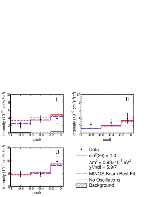
Figure 14: The intensity of neutrino-induced muons as a function of $\cos\theta$. The data are shown by the points, the best fit is shown by the solid line, and the null oscillation hypothesis is shown by the dotted line. The prediction using the MINOS result with the NuMI neutrino beam is shown by the dashed line. The top left panel shows the events with $1<p_{fit}<10$ GeV/$c$ (L), the top right shows the events with $10\leq p_{fit}<100$ GeV/$c$ (H) and the bottom left shows events with unknown momentum (U).

The $N^{\text{MC}}_{i}$ depend on the effects of neutrino oscillations, the systematic uncertainties in the reconstruction and input physics model, and the background present for bin $i$. We define the expected number of muons in bin $i$ as $N^{\text{MC}}_{i}=N^{\text{MC}}_{i}(\sin^{2}2\theta_{23},\Delta m^{2}_{23},\vec{\epsilon})+N^{\text{BG}}_{i}$. The background events due to neutrino interactions inside the detector, $N^{\text{BG}}_{i}$, have been oscillated with the best fit Super-Kamiokande parameters and $\vec{\epsilon}=(\epsilon_{1},\ldots,\epsilon_{7})$ correspond to the uncertainties listed in Table 4. We calculated the values of $\chi^{2}$ at each point on a grid in $(\sin^{2}2\theta_{23},\Delta m^{2}_{23})$ space. The fit varied the $\epsilon_{k}$ at each point to find the minimum $\chi^{2}$ Press et al. (1992) in Eq. (4) Ashie et al. (2005).

IV.3.2 Results of Oscillation Fit

The best fit in the physical region is found at $\sin^{2}2\theta_{23}=1$ and $\Delta m^{2}_{23}=0.93\times 10^{-3}$ eV² with $\chi^{2}/ndf=5.9/7$. The values of the $\epsilon_{k}$ were all found to be less than $1\sigma_{k}$. The results of the fit are shown in Fig. 14, where the best fit to the data in the physical region (solid line), the Monte Carlo prediction for the null oscillation hypothesis (dotted line), and the prediction derived from the MINOS result with the NuMI neutrino beam (dashed line) Michael et al. (2006b) are superposed onto the observed intensity of neutrino-induced muons. For the results from the null oscillation hypothesis and the MINOS beam analysis we varied the $\epsilon_{k}$ to minimize Eq. (4) at the fixed values of $\sin^{2}2\theta_{23}$ and $\Delta m^{2}_{23}$.

Fig. 15 shows the 68% and 90% confidence intervals for the oscillation parameter fit. The points within the 68% contour have a difference in $\chi^{2}$ with the best fit point, $\Delta\chi^{2}$, of less than 2.3. The points within the 90% contour have $\Delta\chi^{2}<4.61$. The null oscillation hypothesis has $\Delta\chi^{2}=5.5$ and is excluded at the $94$% confidence level. Also shown in Fig. 15 is the 90% confidence interval for the MINOS contained vertex analysis Adamson et al. (2006a) based on the first 418 days of data taking with the far detector. The results of these two analyses are consistent.

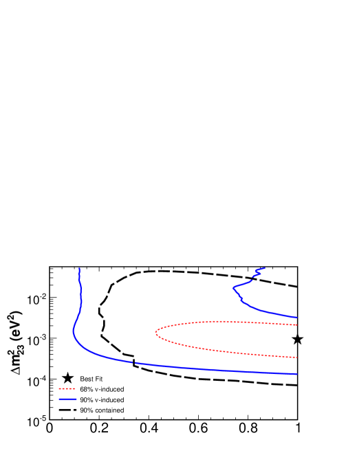
Figure 15: The the 68% (dotted line) and 90% (solid line) confidence intervals for the oscillation parameter fit. The best fit point is indicated by the star. Also shown is the 90% confidence interval for the MINOS contained vertex analysis (dashed line) based on the first 418 days of data taking with the far detector.

V Tests of CPT Conservation

To probe CPT conservation with MINOS data, we use two tests. After discussing the systematic uncertainties, we first compare the strength of the oscillation signals for the neutrino-induced $\mu^{-}$ and $\mu^{+}$ samples individually. Second, we divide the charge-separated muons into low and high momentum samples and further test for differing rates of neutrino disappearance. We show that this second test is the one that minimizes systematic uncertainties.

V.1 Systematic Uncertainties

Here we discuss the additional sources of systematic uncertainties associated with the CPT analysis. One additional source of systematic uncertainty is due to misidentified charge sign or the charge purity of the data sample. We determined the charge purity systematic by comparing the underground cosmic ray muon charge ratio for events passing the $\chi^{2}_{\text{line}}/ndf$ cut with the charge ratio found by MINOS, $N_{\mu^{+}}/N_{\mu^{-}}=1.371$ Adamson et al. (2006b). For this comparison we divided the cosmic ray muons into two data samples, one with muons having momenta $<30$ GeV/$c$ and the other with momenta in the range 30 – 100 GeV/$c$. For cosmic ray muons in the lower momentum sample, we calculated the difference in the charge ratio to be 0.047, a difference that can be attributed to an impurity of 5%. For cosmic ray muons in the high momentum sample, we calculated the difference in the charge ratio to be 0.12, which can be attributed to an impurity of 14%. By taking a weighted average of these impurities, where the weights are given by the number of neutrino-induced muons in each momentum range, we calculated the impurity in the neutrino-induced muon data to be 6%. Using similar methods we found the weighted average impurity for the neutino-induced Monte Carlo events to be 1%. These weighted impurities are given in Table 5 (4).

There are also additional sources of systematic uncertainty due to the physics model. These arise from uncertainties in the ratios of the $\overline{\nu}_{\mu}$ cross section, $\sigma_{\overline{\nu}_{\mu}}$, to the $\nu_{\mu}$ cross section, $\sigma_{\nu_{\mu}}$, and we estimate the uncertainties to be 9% Auchincloss et al. (1990) for energies $<30$ GeV (9) and 2% Yao et al. (2006d) for energies $>30$ GeV (10). The uncertainty in the ratio of the number of $\nu_{\mu}$ to $\overline{\nu}_{\mu}$ (11) is 1% Barr et al. (2006).

V.2 Charge-Separated Event Ratio

Our first test of CPT conservation comes from the comparison of the ratio of the total number of $\mu^{-}$ events to $\mu^{+}$ events in the data and the Monte Carlo simulation including backgrounds. In the data, this ratio of charge separated muons is given by

$$R^{data}_{\mu^{-}/\mu^{+}}=\sum(N_{\mu^{-}}){\Large/}\sum(N_{\mu^{+}}).$$ (5)

The Monte Carlo ratio is defined in a similar way. If the $\nu_{\mu}$ oscillate with the same parameters as the $\overline{\nu}_{\mu}$ then the ratio of the data and Monte Carlo ratios, $\hat{\mathcal{R}}_{CPT}$, will be consistent with unity. The systematic uncertainties in $\hat{\mathcal{R}}_{CPT}$ are shown in Table 5. This table shows how changes in the default parameters corresponding to the sources of systematic uncertainty changes the value of $\hat{\mathcal{R}}_{CPT}$. The main contributions to the uncertainty in $\hat{\mathcal{R}}_{CPT}$ are the purity, cross section ratio for neutrinos with energies $<30$ GeV, and the ratio of $\nu_{\mu}/\overline{\nu}_{\mu}$. Since the ratio in Eq. (5) is greater than one, more negative than positive muons will be misidentified and the measured charge ratio decreases towards unity. Consequently, charge misidentification leads to a one-sided (positive) error on the measured charge ratio. The uncertainty due to the impurity is $(\Delta\hat{\mathcal{R}}_{CPT})_{4}=0.07$. The cross section ratio for neutrinos with energies $<30$ GeV changes the ratio by $(\Delta\hat{\mathcal{R}}_{CPT})_{9}=\pm 0.04$. The uncertainty in the ratio of the number of $\nu_{\mu}$ to $\overline{\nu}_{\mu}$ corresponds to $(\Delta\hat{\mathcal{R}}_{CPT})_{11}=\pm 0.01$. We find from Table 3 and Table 5

$$\hat{\mathcal{R}}_{CPT}=\frac{R^{data}_{{\mu^{-}}/{\mu^{+}}}}{R^{MC}_{{\mu^{-}}/{\mu^{+}}}}=0.72^{+0.24}_{-0.18}(\text{stat})^{+0.08}_{-0.04}(\text{syst}),$$ (6)

where the statistical uncertainties were calculated using the method for Eq. (3). This value of $\hat{\mathcal{R}}_{CPT}$ is consistent with CPT conservation.

Table 5: Sources of systematic uncertainty considered and their effects on the ratio $\hat{\mathcal{R}}_{CPT}$.

Source	$\sigma$	$(\Delta\mathcal{\hat{R}}_{CPT})_{k}$
Reconstruction systematics:
(1) $\chi^{2}_{fit}/ndf<1.5$	0.01	$<5\times 10^{-4}$
(2) $\chi^{2}_{1/\beta}/ndf<3.0$	0.01	$<1\times 10^{-4}$
(3) $\chi^{2}_{\text{line}}/ndf<10$	0.27	$<5\times 10^{-3}$
(4) Charge Purity (Data,MC)	(0.06,0.01)	+0.07
Model systematics:
(5) Normalization	0.15	$<1\times 10^{-4}$
(6) Spectral Index	0.03	$<1\times 10^{-4}$
(7) Cross Section ($E<30$ GeV)	0.07	$<5\times 10^{-3}$
(8) Cross Section ($E>30$ GeV)	0.02	$<5\times 10^{-3}$
(9) $\sigma_{\overline{\nu}_{\mu}}/\sigma_{\nu_{\mu}}$ ($E<30$ GeV)	0.09	0.04
(10) $\sigma_{\overline{\nu}_{\mu}}/\sigma_{\nu_{\mu}}$ ($E>30$ GeV)	0.02	$<5\times 10^{-3}$
(11) $\nu_{\mu}/\overline{\nu}_{\mu}$	0.01	0.01
$\Delta\mathcal{\hat{R}}_{CPT}=\sqrt{\sum(\Delta\mathcal{\hat{R}}_{CPT})_{k}^{2}}$		-0.04, +0.08

V.3 Charge-Separated, Low-to-High Momentun Event Ratio

Our second test of CPT conservation is based on the charge separated ratios of low momentum to high momentum events compared to the Monte Carlo expectation including backgrounds. First define ratios of data to Monte Carlo expectation for the $\nu_{\mu}$ and $\overline{\nu}_{\mu}$ individually,

$${\cal R}_{-} = \biggl{(}\frac{R^{data}_{{L}/{H}}}{R^{MC}_{{L}/{H}}}\biggr{)}_{\mu^{-}}$$ (7)

$$= 0.49^{+0.20}_{-0.14}(\text{stat})\pm 0.07(\text{syst}),$$

and

$${\cal R}_{+} = \biggl{(}\frac{R^{data}_{{L}/{H}}}{R^{MC}_{{L}/{H}}}\biggr{)}_{\mu^{+}}$$ (8)

$$= 0.55^{+0.30}_{-0.19}(\text{stat})\pm 0.07(\text{syst}).$$

The systematic uncertainties in these ratios are listed in Table 6, and the statistical uncertainties were again calculated using the same method as for Eq. (3). We define the ratio of ratios $\tilde{\mathcal{R}}_{CPT}$,

$$\tilde{\mathcal{R}}_{CPT}={\cal R}_{-}/{\cal R}_{+}=0.89^{+0.54}_{-0.33}(\text{stat})\pm 0.03(\text{syst}).$$ (9)

We found the upper and lower limits for the statistical uncertainty in Eq. (9) by fitting the observed L and H event rates for $\mu^{-}$ and $\mu^{+}$ to a model which used $\tilde{\mathcal{R}}_{CPT}$ and three of the four event rates as inputs. The data and model were compared using a $\chi^{2}$ function appropriate for Poisson distributed data Yao et al. (2006c). The 68% C. L. interval quoted includes all values of $\tilde{\mathcal{R}}_{CPT}$ which produce a $\chi^{2}$ within 1 of the best fit value. Again within the statistical and systematic uncertainties, the value of $\tilde{\mathcal{R}}_{CPT}$ is consistent with unity and CPT conservation.

The value of this test is clearly demonstrated in Table 6 where it can be seen that several sources of systematic uncertainty cancel in the calculation of $\tilde{\mathcal{R}}_{CPT}$. These cancellations occur because the $\mu^{-}$ and $\mu^{+}$ ratios are affected similarly for these systematic uncertainties and so divide out in the ratio. The uncertainty in the ratio of the number of $\nu_{\mu}$ to the number of $\overline{\nu}_{\mu}$ does not contribute to the uncertainty in $\tilde{\mathcal{R}}_{CPT}$. As seen in Table 6, the only sources of uncertainty which do not cancel are those in the relative magnitude of the $\nu_{\mu}$ and $\overline{\nu}_{\mu}$ cross sections at low (9) and high (10) energies.

This approach should prove valuable in high statistics accelerator-based tests of CPT conservation because it minimizes systematic uncertainties so effectively.

Table 6: Sources of systematic uncertainty considered and their effects on the ratios $\mathcal{R_{-}}$, $\mathcal{R_{+}}$, and $\mathcal{\tilde{R}_{CPT}}$.

Source	$\sigma$	$\Delta\mathcal{R}_{-}$		$\Delta\mathcal{R}_{+}$		$(\Delta{\mathcal{\tilde{R}}_{CPT}})_{k}$
		$-1\sigma$	$+1\sigma$	$-1\sigma$	$+1\sigma$
Reconstruction systematics:
(1) $\chi^{2}_{fit}/ndf<1.5$	0.01	$<5\times 10^{-4}$	$<5\times 10^{-4}$	$<5\times 10^{-4}$	$<5\times 10^{-4}$	–
(2) $\chi^{2}_{1/\beta}/ndf<3.0$	0.01	$<1\times 10^{-4}$	$<1\times 10^{-4}$	$<1\times 10^{-4}$	$<1\times 10^{-4}$	–
(3) $\chi^{2}_{\text{line}}/ndf<10$	0.27	0.05	0.05	0.05	0.05	–
(4) Charge Purity (Data,MC)	(0.06,0.01)	$<1\times 10^{-4}$	$<1\times 10^{-4}$	$<1\times 10^{-4}$	$<1\times 10^{-4}$	–
Model systematics:
(5) Normalization	0.15	$<1\times 10^{-4}$	$<1\times 10^{-4}$	$<1\times 10^{-4}$	$<1\times 10^{-4}$	–
(6) Spectral Index	0.03	0.04	0.03	0.04	0.04	–
(7) Cross Section ($E<30$ GeV)	0.07	0.02	0.02	0.02	0.02	–
(8) Cross Section ($E>30$ GeV)	0.02	0.01	0.01	0.01	0.01	–
(9) $\sigma_{\overline{\nu}_{\mu}}/\sigma_{\nu_{\mu}}$ ($E<30$ GeV)	0.09	–	–	0.02	0.02	0.03
(10) $\sigma_{\overline{\nu}_{\mu}}/\sigma_{\nu_{\mu}}$ ($E>30$ GeV)	0.02	–	–	0.01	0.01	0.01
$\Delta{\mathcal{\tilde{R}}}_{CPT}=\sqrt{\sum(\Delta{\mathcal{\tilde{R}}}_{CPT})_{k}^{2}}$						$0.03$

VI Conclusions

The MINOS far detector has taken $854.24$ days of data in its search for the atmospheric neutrino-induced muons. We found a total of $140$ neutrino-induced muons in the data set. We have performed four analyses. The ratio of the number of low momentum muons to the sum of high momentum and unknown momentum muons has been compared to the same ratio for Monte Carlo events. The resulting ratio, ${\cal R}$, suggests neutrino disappearance at the $2.0\sigma$ level. The best oscillation fit to the data gives $\sin^{2}2\theta_{23}=1.0$ and $\Delta m^{2}_{23}=0.93\times 10^{-3}$ eV². This fit excludes the null oscillation hypothesis at the $94$% confidence level. We used two methods to look for evidence of different rates of neutrino disappearance as a test of CPT conservation. Both tests are consistent with CPT conservation. The cancellation of many systematic uncertainties in the computation of $\tilde{\mathcal{R}}_{CPT}$ suggests that this test would provide a precision test of CPT conservation with a suitably large dataset.

Acknowledgments

We thank the Fermilab staff and the technical staffs of the participating institutions for their vital contributions. This work was supported by the U.S. Department of Energy, the U.S. National Science Foundation, the U.K. Particle Physics and Astronomy Research Council, the State and University of Minnesota, the Office of Special Accounts for Research Grants of the University of Athens, Greece, FAPESP (Rundacao de Amparo a Pesquisa do Estado de Sao Paulo), CNPq (Conselho Nacional de Desenvolvimento Cientifico e Tecnologico) in Brazil, and the computational resources of the AVIDD cluster at Indiana University. We gratefully acknowledge the Minnesota Department of Natural Resources for their assistance and for allowing us access to the facilities of the Soudan Underground Mine State Park. We also thank the crew of the Soudan Underground Physics laboratory for their tireless work in building and operating the MINOS detector.

References

- Fukuda et al. (1998a) Y. Fukuda et al. (Super-Kamiokande), Phys. Lett. B 433, 9 (1998a), eprint hep-ex/9803006.
- Fukuda et al. (1998b) Y. Fukuda et al. (Super-Kamiokande), Phys. Rev. Lett. 81, 1562 (1998b), eprint hep-ex/9807003.
- Fukuda et al. (1998c) Y. Fukuda et al. (Super-Kamiokande), Phys. Lett. B 436, 33 (1998c), eprint hep-ex/9805006.
- Fukuda et al. (1999a) Y. Fukuda et al. (Super-Kamiokande), Phys. Lett. B 467, 185 (1999a), eprint hep-ex/9908049.
- Fukuda et al. (1999b) Y. Fukuda et al. (Super-Kamiokande), Phys. Rev. Lett. 82, 2644 (1999b), eprint hep-ex/9812014.
- Fukuda et al. (2000) S. Fukuda et al. (Super-Kamiokande), Phys. Rev. Lett. 85, 3999 (2000), eprint hep-ex/0009001.
- Ashie et al. (2004) Y. Ashie et al. (Super-Kamiokande), Phys. Rev. Lett. 93, 101801 (2004), eprint hep-ex/0404034.
- Ashie et al. (2005) Y. Ashie et al. (Super-Kamiokande), Phys. Rev. D 71, 112005 (2005), eprint hep-ex/0501064.
- Abe et al. (2006) K. Abe et al. (Super-Kamiokande) (2006), submitted to Phys. Rev. Lett., eprint hep-ex/0607059.
- Yao et al. (2006a) W. Yao et al. (Particle Data Group), J. Phys. G 33, 1 (2006a), see B. Kayser, 13. Neutrino Mass, Mixing, and Flavor Change, p.156.
- Kayser (2004) B. Kayser, in Proceedings of the 32nd SLAC Summer Institute on Particle Physics (Menlo Park, CA, 2004), p. L004, eprint hep-ph/0506165.
- (12) More precisely, the experiment measures where effects of order have been neglected; see H. Nunokawa, S. J. Parke, and R. Zunkanovich Funchal, Phys. Rev. D, 72, 013009 (2005), hep-ph/0503283.
- Ambrosio et al. (2001) M. Ambrosio et al. (MACRO), Phys. Lett. B 517, 59 (2001).
- Ambrosio et al. (2004) M. Ambrosio et al. (MACRO), Eur. Phys. J. C 36, 323 (2004).
- Sanchez et al. (2003) M. C. Sanchez et al. (Soudan 2), Phys. Rev. D 68, 113004 (2003), eprint hep-ex/0307069.
- Allison et al. (2005) W. W. M. Allison et al. (Soudan 2), Phys. Rev. D 72, 052005 (2005), eprint hep-ex/0507068.
- Adamson et al. (2006a) P. Adamson et al. (MINOS), Phys. Rev. D 73, 072002 (2006a).
- Michael et al. (2006a) D. G. Michael et al., Nucl. Instrum. Methods Phys. Res. Sect. B (2006a), to be submitted.
- Michael et al. (2006b) D. Michael et al. (MINOS), Phys. Rev. Lett. 97, 191801 (2006b), eprint hep-ex/0607088.
- Aliu et al. (2005) E. Aliu et al. (K2K), Phys. Rev. Lett. 94, 081802 (2005), eprint hep-ex/0411038.
- Ahn et al. (2006) M. Ahn et al. (K2K), Phys. Rev. D 74, 072003 (2006), eprint hep-ex/0606032.
- Apollonio et al. (1999) M. Apollonio et al. (CHOOZ), Phys. Lett. B 466, 415 (1999), eprint hep-ex/9907037.
- Palomares-Ruiz and Petcov (2005) S. Palomares-Ruiz and S. T. Petcov, Nucl. Phys. B 712, 392 (2005), eprint hep-ph/0406096.
- Border et al. (2001) P. Border et al., Nucl. Instrum. Meth. A 463, 194 (2001).
- Rebel (2004) B. J. Rebel, Ph.D. thesis, Indiana University (2004).
- Blake (2005) A. Blake, Ph.D. thesis, Cambridge University (2005).
- Agrawal et al. (1996) V. Agrawal, T. K. Gaisser, P. Lipari, and T. Stanev, Phys. Rev. D 53, 1314 (1996).
- Casper (2002) D. Casper, Nucl. Phys. B Proc. Suppl. 112, 161 (2002).
- Gluck et al. (1995) M. Gluck, E. Reya, and A. Vogt, Z. Phys. C 67, 433 (1995).
- Kasahara (1997) S. M. S. Kasahara, Ph.D. thesis, University of Minnesota (1997).
- Yao et al. (2006b) W. Yao et al. (Particle Data Group), J. Phys. G 33, 1 (2006b), see T.K. Gaisser and T. Stanev, 24. Cosmic Rays, p.245.
- Hawthorne (1997) A. M. Hawthorne, Ph.D. thesis, Indiana University (1997).
- Adamson et al. (2006b) P. Adamson et al. (MINOS) (2006b), to be submitted to Phys. Rev. D.
- Gaisser (1990) T. K. Gaisser, Cosmic Rays and Particle Physics (Cambridge University Press, 1990).
- Barr et al. (2006) G. D. Barr, T. K. Gaisser, S. Robbins, and T. Stanev, Phys. Rev. D 74, 094009 (2006), eprint astro-ph/0611266.
- Auchincloss et al. (1990) P. S. Auchincloss et al. (CCFR), Z. Phys. C 48, 411 (1990).
- Gehrels (1986) N. Gehrels, Astrophys. J. 303, 336 (1986).
- Yao et al. (2006c) W. Yao et al. (Particle Data Group), J. Phys. G 33, 1 (2006c), see G. Cowan, 32. Statistics, p.301.
- Press et al. (1992) W. H. Press, B. Flannery, S. Teukolsky, and W. Vetterling, Numerical Recipes in C (Cambridge University Press, 1992).
- Yao et al. (2006d) W. Yao et al. (Particle Data Group), J. Phys. G 33, 1 (2006d), see, 40. Plots of cross sections and related quantities, p.336.