Abstract

A technique to measure low intensity fast neutron flux has been developed. The design, calibrations, procedure for data analysis and interpretation of the results are discussed in detail. The technique has been applied to measure the neutron background from rock at the Boulby Underground Laboratory, a site used for dark matter and other experiments, requiring shielding from cosmic ray muons. The experiment was performed using a liquid scintillation detector. A 6.1 litre volume stainless steel cell was filled with an in-house made liquid scintillator loaded with Gd to enhance neutron capture. A two-pulse signature (proton recoils followed by gammas from neutron capture) was used to identify the neutron events from much larger gamma background from PMTs. Suppression of gammas from the rock was achieved by surrounding the detector with high-purity lead and copper. Calibrations of the detector were performed with various gamma and neutron sources. Special care was taken to eliminate PMT afterpulses and correlated background events from the delayed coincidences of two pulses in the Bi-Po decay chain. A four month run revealed a neutron-induced event rate of $1.84\pm 0.65(stat.)$ events/day. Monte Carlo simulations based on the GEANT4 toolkit were carried out to estimate the efficiency of the detector and the energy spectra of the expected proton recoils. From comparison of the measured rate with Monte Carlo simulations the flux of fast neutrons from rock was estimated as $(1.72\pm 0.61(stat.)\pm 0.38(syst.))\times 10^{-6}$ cm^-2 s^-1 above 0.5 MeV.

Keywords: Neutron background; Spontaneous fission; ($\alpha$,n) reactions; Radioactivity; Dark matter; Underground physics

PACS: 95.35.+d; 29.40.Mc; 25.55.-e; 28.20.-v

Corresponding author: E. Tziaferi, Department of Physics and Astronomy, University of Sheffield, Hicks Building, Hounsfield Road, Sheffield S3 7RH, UK

Tel: +44 (0)114 2223547;                   Fax: +44 (0)114 2223555;

E-mail: e.tziaferi@sheffield.ac.uk

1 Introduction

Neutrons are the most important background for a large variety of underground experiments. Experiments searching for Weakly Interacting Massive Particles (WIMPs), for example, work with a very low energy threshold, and are sensitive to (and should be protected from) neutrons from all possible sources: rock, detector, shielding components and cosmic-ray muons. Neutrons, like WIMPs, induce nuclear recoils, so it is crucial that the neutron flux is suppressed by shielding, active veto systems and the use of ultra-pure materials.

The neutron flux from rock dominates over other sources. It originates in spontaneous fission (mainly ²³⁸U) and ($\alpha$,n) reactions due to uranium and thorium traces. The suppression of this flux can be achieved by installing hydrocarbon shielding around the detector. The required thickness of the shielding is determined by the neutron flux and the projected sensitivity of the WIMP dark matter detector. The neutron flux from rock and its effect on the detector sensitivity can be calculated using the measured contamination levels of U and Th. However, there may be quite a large uncertainty in such a calculation. Firstly, the cross-sections of ($\alpha$,n) reactions are not known with high precision for a large number of isotopes, in particular the energy spectra of emitted neutrons are quite uncertain. Secondly, Monte Carlo codes for neutron transport need to be extensively tested and should use the most accurate libraries for neutron interaction cross-sections. Thirdly, measurements of U/Th concentrations may not provide accurate results for the actual concentrations present. If such measurements are done using mass-spectrometry, then only a few samples can be tested and further studies then rely on the assumption of a uniform concentration of U/Th in the rock. If they are performed with a Ge detector, then the gamma lines provide an estimate of concentration of certain isotopes in the U/Th decay chains and the evaluation of the neutron flux depends then on the assumption that there is equilibrium in these chains. Obviously an accurate calibration of the Ge detector is also necessary. Finally, the exact composition of the rock may not be known to a high degree of accuracy. For example, the fraction of water (hydrogen) may vary and is anyway difficult to measure. Meanwhile, hydrogen (even 1% of H) affects dramatically the moderation and absorption of neutrons [1, 2]. So direct measurements of the neutron flux from rock is important as a means of checking the calculations based on other U/Th concentration measurements.

The Boulby Underground Laboratory situated at a vertical depth of 1070 m underground (2800  m w.e. [3]) hosts several dark matter experiments [4, 5, 6, 7]. The concentrations of U and Th in Boulby rock which is almost pure NaCl salt (surrounding the underground laboratory), were evaluated from measurements of gamma lines associated with U/Th decay chains [8]. A Ge detector was exposed to the gamma flux from the rock surrounding the laboratory hall and the intensitities of the observed gamma lines were converted into U/Th concentration levels using Monte Carlo simulations [8].

In this paper we discuss our technique to measure low-intensity neutron fluxes and the application of this technique to the study of the neutron background from rock at Boulby mine. The detector, scintillator and data aquisition system (DAQ) are described in Section 2. Detector calibrations are presented in Section 3. Our measurements of neutron flux from the rock are described in Section 4. The results of the experiment are shown and the uncertainties are discussed in Section 5. Finally the conclusions are given in Section 6.

2 Detector and DAQ

The liquid scintillation detector used in the experiment consisted of a cylindrical stainless steel vessel 19.7 cm diameter and 20.0 cm length filled with a liquid scintillator based on diisopropylnaphthalene (C₁₆H₂₀) of volumic density 0.97 g/cm³, loaded with $\sim$0.2% of Gd to increase the probability of neutron capture. The recipe used for Gd loading is similar to that described in Ref. [9] where much higher loading of Gd had been achieved. The attenuation length of the scintillator was measured to be about 5 metres, well exceeding the size of the detector. The scintillator has a high flash-point (more than 100^∘C) and low-toxicity - requirements imposed by health and safety considerations of a working mine.

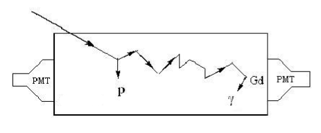
Figure 1: Detection principle: A neutron entering the detector produces proton recoils by elastic scattering, then slows down, is thermalised and finally captured with the emission of gammas.

The two flat surfaces of the detector were viewed by two 5” fast Hamamatsu photomultiplier tubes (PMTs) through quartz windows, attached with optical coupling grease (Figure 1). The inner surface of the vessel, including the two rings around the quartz windows, were coated with aluminised mylar with a coefficient of reflection greater than 0.9 to maximise light collection.

The detector was running in an environment with a temperature of more than 30^oC, so a cooling system was installed to prevent degradation of the scintillator. Copper coils were wrapped around the vessel and running water, from a chiller, enabled the temperature to be maintained at about 20^oC.

The detector was installed inside a ‘castle’ made of ultra-pure copper and lead and N₂ was bubbled through the scintillator to remove dissolved oxygen. The temperatures of the scintillator (about 20^oC), the castle (26^oC) and the ambient air (30-33^oC) were measured with thermocouples. The thickness of lead and copper in the ‘castle’ was 7.5 and 10 cm, respectively, for the top and three vertical sides of the castle. For the bottom part and one vertical side the thickness of lead was 15 cm. Lead and copper shielding ensures the suppression of the gamma flux from the rock by several orders of magnitude. For energy calibrations with gamma sources a hole was made in the roof of the castle into which a source could be inserted. With the hole plugged none of the gamma sources could be detected. The configuration of the detector with shielding and the rest of the environment was included in our Monte Carlo code to simulate the detector response to various radiations.

Two different DAQ circuits were used: one for gamma calibration (giving 1 pulse) and one for neutron measurement (giving 2 pulses in delayed coincidences), see Figure 2. For all runs, the signals from both PMTs were fed into NIM low-threshold discriminator units set to trigger when the signal exceeded a threshold of 10 mV, equivalent to 2 photoelectrons from each tube. For energy calibration runs, the logic signals from the discriminator channels were fed into a coincidence unit which triggered the waveform digitisers (CompactPCI Acqiris digitiser) when signals arrived from the two PMTs (time gate 150 ns). When the waveform digitiser was triggered, the signals from both PMTs were digitised (sampling rate 0.5 GHz, digitisation accuracy 2 ns, total digitisation time 200 ns), passed to a computer and stored on disk for off-line analysis.

For neutron measurements and calibrations, the output signal of the coincidence unit was split in two, one fed into the second coincidence unit and the other sent to two timers sequentially. The first timer gave a 1.8 $\mu$s delay and the second timer opened a time gate of 200 $\mu$s. The gate from the second timer was sent to the second coincidence unit and this unit generated a trigger if the second pulse arrived within the 200 $\mu$s time gate. The trigger was sent to the digitiser and the signals from the PMTs were digitised in the same way as described above but the total digitisation time was 200 $\mu$s. Such a scheme thus enabled detection of two pulses - the first one assumed to be from proton recoils induced by neutron elastic scattering and the second one due to the Compton electrons produced by gammas from neutron capture on Gd, H or other elements. The first timer with 1.8 $\mu$s delay was needed to avoid triggering on the 1st pulse twice (the 2nd pulse should be delayed relative to the 1st one by a certain time).

3 Calibrations

To characterise the detector and its response to various radiations the following calibrations were carried out:

1. Energy calibration using gamma-rays from ⁵⁷Co, ¹³⁷Cs and ⁶⁰Co radioactive sources.

2. Calibration with neutrons from a ²⁵²Cf neutron source with the detection of delayed coincidences to demonstrate the sensitivity of the detector to neutrons and to check efficiency.

3. Calibration with gamma-rays from ⁶⁰Co source with the detection of delayed coincidences to show that these coincidences produce a random background – not connected to neutrons or any spurious effects.

In the absence of photoelectric peaks from gamma-ray lines in light materials, the energy calibration of the detector was performed using the Compton edges of the energy spectra of events from different sources. Due to the finite energy resolution of the detector the Compton edge was smeared out and accurate calibration was possible only by comparing the measured energy distribution with simulations. Simulations were carried out using the GEANT4 toolkit [10] taking into account the configuration of the detector, shielding and the position of the source. The simulated spectrum of energy depositions was convolved with the energy resolution of the detector assumed to be Gaussian with standard deviation of the form $(\sigma/E)^{2}=\alpha+\beta/E$ [11]. The parameters $\alpha$ and $\beta$, as well as the conversion factor from the measured charge to the energy scale, were determined from a comparison with the measured spectrum.

Three gamma-ray sources were used for energy calibration: ⁵⁷Co (most intense gamma-ray line at 122 keV, 40 keV Compton edge), ¹³⁷Cs (622 keV gamma-ray line, 480 keV Compton edge) and ⁶⁰Co (1173 keV and 1332 keV gamma-ray lines, about 1040 keV mean energy for the Compton edges). The ⁵⁷Co source has a Compton edge very close to the energy threshold of the detector. In this case the Compton edge could be confused with (and/or superimposed on) the threshold effect. To avoid errors, the energy spectrum from this source was used only to check the energy calibration with other sources. The calibrations with all sources showed consistent results with the values of $\alpha$ = 0.08 and $\beta$ = 3.9 keV if $E$ is measured in keV.

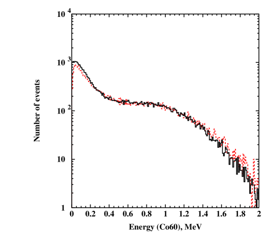
Figure 3: Energy spectrum of events from ⁶⁰Co: data (dashed histogram) and GEANT4 simulations (solid histogram).

Energy calibration of the detector with different sources was carried out regularly with time intervals of 1 - 2 months and the conversion factor found to be stable within 10% over the 4 month running time of the experiment. An average value was used in the analysis. Possible uncertainties in the conversion factor and energy resolution and their effects on the neutron flux measurements are discussed in Section 5. An example of the spectrum of energy depositions from ⁶⁰Co is shown in Figure 3.

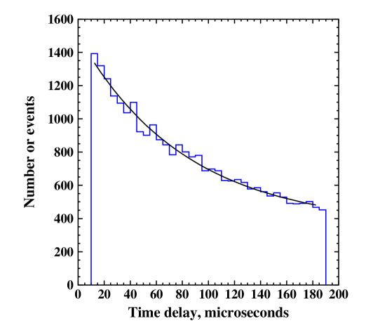
Figure 4: Distribution of time delay between the 1st (proton recoils) and 2nd (neutron capture) pulses in events from ²⁵²Cf data. A fit with a sum of an exponential and a constant is also shown with a solid curve.

Neutrons from spontaneous fission of ²⁵²Cf were used to test if the detector was sensitive to neutrons and to estimate the efficiency of the detector. The source produced a total rate of about 13000 neutrons per second and was positioned either at a distance of about 1 m from the detector or on top of the ’castle’. As described in Section 2 the DAQ was configured to detect two pulses in delayed coincidence within a time window of 200 $\mu$s – the first pulse due to proton recoils from neutron elastic scattering and the second due to gammas from neutron capture. As the incident neutron flux from the ²⁵²Cf source is very high, there was a non-zero probability of detecting random coincidences within 200 $\mu$s between two pulses produced by proton recoils from two neutrons or two pulses produced by gammas from two captured neutrons. Figure 4 shows the time delay distribution of the two pulses. In the calibration the presence of random coincidences described above adds a flat distribution superimposed on the exponential. (Strictly speaking the component due to random coincidence should also be exponential, but since the mean time between two random pulses always exceeded 4 ms, this exponential can be approximated by a constant on a time scale of 200 $\mu$s.) Each distribution was fitted with the two-component function $N=N_{n}/\tau\times\Delta t\times\exp(-t/\tau)+N_{b}$ with 3 free parameters: the number of background events per time bin $N_{b}$, the mean time delay (index of the exponential) $\tau$ and the total number of neutrons $N_{n}$. In the formula above, $\Delta t$ denotes the width of the time bin and $N$ denotes the number of events per bin. Note that $N_{n}$ is the total number of neutrons integrated over all time delays, so a correction for reduced efficiency due to reduced range of time delays is not needed. The index of the exponential was found using a fit to the neutron calibration data which had the highest statistics: $\tau=84.21\pm 5.50$ $\mu$s.

The rate of delayed coincidences between proton recoils and gammas from neutron capture was found to be $5.87\pm 0.68$ s^-1 and $0.53\pm 0.04$ s^-1 during the calibration run having the source on top of the ’castle’ and 1 m away respectively (for 50 keV energy threshold for the 1st pulse and 100 keV threshold for the 2nd pulse – the reasons for these thresholds will be given below).

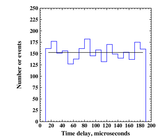
Figure 5: Distribution of time delay between the 1st and 2nd pulses in events from ⁶⁰Co source due to random coincidences between gammas. A fit with a constant function is also shown with a solid curve.

In addition, a calibration run with the ⁶⁰Co source was carried out with the same DAQ settings as for the run with ²⁵²Cf. The time delay distribution is shown in Figure 5. The presence of the two pulses in an event in this case is due to random concidences of two gammas within a time window of $200$ $\mu$s. The time delay distribution is flat proving that the exponential shape observed with the neutron source is not an effect of DAQ but is due to neutron events. The results from these calibrations proved that the detector was sensitive to neutrons and allowed the efficiency of neutron detection to be calculated.

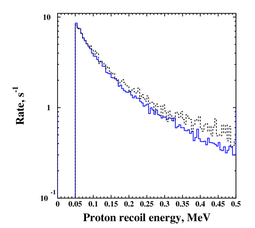
Figure 6: Proton recoil spectra (rates in absolute units per 5 keV without any normalisation) from data (dashed histogram) and GEANT4 simulations (solid histogram) of ²⁵²Cf run.

Finally, a ²⁵²Cf run was carried out having the same DAQ settings as for the energy calibration runs, recording single pulses (mainly proton recoils with some admixture of gammas), without delayed coincidences. The energy spectrum of proton recoils as measured with the neutron source on top of the castle is shown in Figure 6 (dashed line). Also the corresponding spectrum (without any normalisation) calculated with GEANT4 (solid line) is shown, taking into account typical quenching of scintillations for protons in organic liquid scintillators [12] in the form: $E=0.2E_{p}^{1.53}$, where $E_{p}$ is the kinetic energy of a proton in MeV and $E$ is the measured energy in MeV relative to the high-energy gamma calibration point from the ⁶⁰Co source. The small difference, at high energies between the measured and simulated spectra is likely due to the presence of gammas from neutron capture in the calibration data (see the explanation above). In the simulation no neutron captures were included. The measured rate was $163.88\pm 1.40$ s^-1 and the simulated one was 140.30 s^-1, for the energy range of 50-500 keV. This agreement allows us to conclude that GEANT4 simulates neutron transport and production of proton recoils with reasonable accuracy. The uncertainty can be estimated from the difference between measured and simulated rates which is 14%. This is consistent with the conclusion of Ref. [1] that claims a good agreement between GEANT4 [10], MCNPX [13, 14] and GEANT3 [15] for neutron propagation through large thicknesses of rock and shielding.

The calibration runs described above allowed determination of the conversion factor between the detected charge and the energy of particles (electron equivalent energy), the energy resolution of the detector, the energy threshold and the trigger efficiency as a function of measured energy (the later is discussed in Section 5). The results of these runs proved that the detector is sensitive to neutrons and that the Monte Carlo simulations using the GEANT4 toolkit were able to reproduce the energy spectrum and absolute rate of proton recoils. Comparison between the measured rate of delayed coincidences and the measured/calculated rates of single proton recoils allowed us to estimate the efficiency of detecting delayed coincidences (see below).

4 Measurements of the neutron flux from rock

The experiment to measure the neutron flux at the Boulby Undergound Laboratory was carried out from November 2004 to September 2005. The first three months of the experiment were dedicated to studying the behaviour of the detector and its background. Measurement of the neutron flux from the rock were performed between the end of February 2005 and the end of June 2005. During that time all DAQ settings remained the same and the run was interrupted only to carry out various calibrations of the detector to ensure its stability.

The neutron flux from salt rock was expected to be quite low requiring sensitive equipment for its measurement. An important part of the experiment was the study and rejection of background events which might be an obstacle for such a sensitive measurement.

Two important sources of background events producing delayed coincidences were found in this experiment. The first are afterpulses from the PMTs, known to occur up to a few microseconds after the main pulse from the PMT. Their amplitude normally does not exceed a few photoelectrons, which is equivalent to a few tens of keV for our detector. The probability of having two afterpulses from the two PMTs during the 150 ns coincidence gate used here is very low, however the experiment in fact does have a low signal rate, the total rate being a few tens of events per day. The rate of random coincidences between afterpulses and/or noise pulses may not be negligible compared to the signal rate. A histogram of time differences between two secondary pulses from the two PMTs for such events is flat showing that secondary pulses from the two PMTs are not correlated but are due to random coincidences between afterpulses and/or noise pulses from different PMTs. Thus, such a background is due to the delayed coincidence of the following pulses: first pulse - normal scintillation pulse on both PMTs; second pulse - afterpulses and/or noise pulses on two PMTs. The rejection of this background was done by requiring the second pulse to have an amplitude of more than 100 keV and to be delayed by more than 10 $\mu$s relative to the first pulse. The fraction of events from ²⁵²Cf which passed the above cut is (75 $\pm$ 1)%. Such a cut limits the sensitivity of the detector to neutrons. The same cut was applied to data and calibration run with ²⁵²Cf and its efficiency was automatically included in the overall efficiency of detecting the second pulse in an event. This efficiency does not depend on the source of neutrons, either Cf or rock, because this cut removes only second pulses induced by gammas from neutron captures, whose spectrum does not depend on the neutron source.

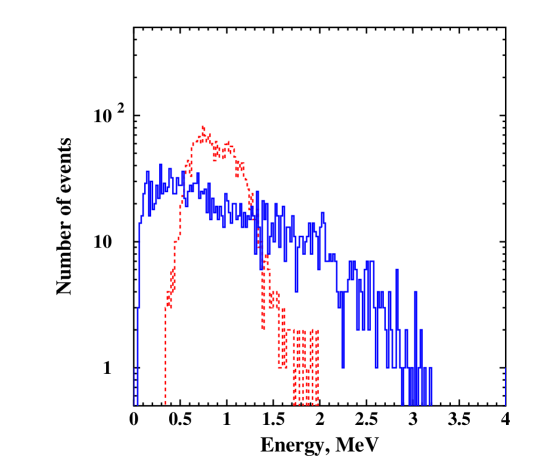
Figure 7: Measured energy spectra of the first pulse (solid histogram) from beta emission and the second pulse (dashed histogram) from alpha decay, for the correlated background due to the Bi$\rightarrow$Po$\rightarrow$Pb decay.

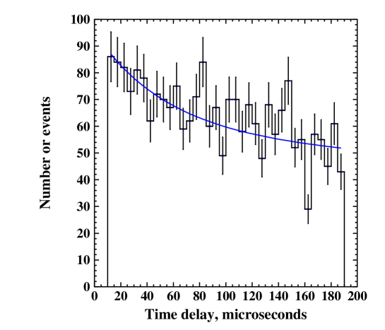
Figure 8: Measured distribution of the time delay between the first (from beta emission) and second (from alpha decay) pulses in the events from the correlated background due to the Bi$\rightarrow$Po$\rightarrow$Pb decay. The solid curve is the fit with an exponential of 237 $\mu$s.

The second source of background arises from the possibility of two consecutive decays in the ²³⁸U decay chain: ²¹⁴Bi$\rightarrow^{214}$Po $\rightarrow^{210}$Pb. The first decay goes via beta emission whereas the second one is an alpha-decay. The half-life of ²¹⁴Po is 164 $\mu$s which makes the two pulses from this decay chain capable of mimicking the signal from neutrons. Prior to installation of the detector, the scintillator was exposed to air with a certain concentration of radon. Radon daughters were diffused in the scintillator and at the beginning of the running time (November – December 2004) the rate of correlated background events from Bi$\rightarrow$Po$\rightarrow$Pb decays was quite high (the rate on the first day was 324 $\pm$ 18 events/day). Figure 7 shows the energy spectra of the first and second pulses in the events from this correlated background. The energy spectrum of the second pulse has a clear peak at about 0.8 MeV – quenched peak of alphas at 7.68 MeV. Note that the expected alpha peak, taking into account the quenching of alphas in standard liquid scintillator, should be at about 0.96 MeV [19], in a reasonable agreement with the measured value. The difference between the measured value for the peak position and the predictions can be used to estimate the uncertainty in the energy scale for proton recoils (see Section 5). Figure 8 shows the distribution of the time delay between the first and second pulses in the events from the correlated background. It is well fitted with an exponential of 237 $\mu$s consistent with the origin of this background being due to the Bi$\rightarrow$Po$\rightarrow$Pb decays.

Figure 9 shows the rate of correlated background events as a function of time since the beginning of the experiment in November 2004. The rate dropped to a few events per day after 1 month of operation. The remaining events are due to intrinsic contamination of scintillator and/or vessel walls by uranium (note only isotopes in a few microns of the walls in contact with scintillator can produce an alpha pulse in the scintillator). These events can be eliminated using the following cuts. Firstly, the fact that the secondary alpha events are concentrated around 0.8 MeV can be used to reject this background. However, as can be seen from Figure 7 the alpha peak is very broad and many neutron capture events also have energies in this range. Secondly, the correlated background events can be rejected using pulse shape analysis: the second pulses are due to alphas in the correlated background events whereas for neutron events they are due to Compton electrons. The possibility of using pulse shape discrimination can be seen from Figure 10 which shows the ratio of charge in the tail of the pulse (20 to 100 ns since the beginning of the pulse) to the total charge. A population of events due to alphas is clearly seen for tail/total ratio more than 0.2 (for the second pulses in the events – Figure 10b). Pulses due to electrons (first pulse in the background events – Figure 10a) lie mainly below 0.3 at energies above 0.5 MeV. For further analysis only events with second pulses which had tail/total ratio of less than 0.2 in the energy region of 0.35 - 2.00 MeV were used. Again, to estimate the efficiency of this selection criterium, the same cut was applied to the neutron calibration data. As only pulses from the neutron capture gammas are affected, the efficiency does not depend on the neutron spectrum.

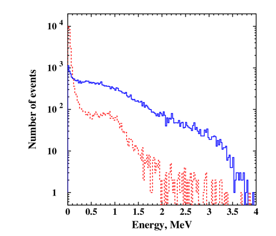
Figure 11: Energy spectra of the first (solid histogram) and the second (dashed histogram) pulses in the events included in the analysis for neutron flux measurements, prior to the applied cuts.

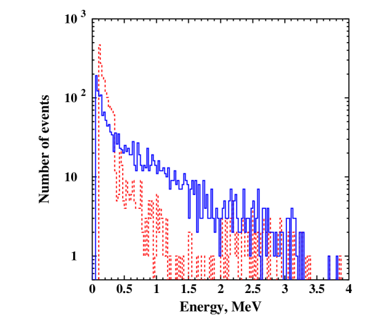
Figure 12: Energy spectra of the first (solid histogram) and the second (dashed histogram) pulses in the events included in the analysis for neutron flux measurements, after the applied cuts.

Data included in the analysis of neutrons from rock were collected during 123 days of live time. After rejection of events from these two sources of background there remained two types of events in the data: neutron events caused by radioactivity in rock and random coincidences of background pulses within a 200 $\mu$s time window. The average rate of events was about 2.0/min, reduced down to about 10 events/day after cuts. The energy spectra of the first and second pulses, for all events included in the analysis, before and after the cuts are shown in Figures 11 and 12 respectively. In addition, the plots of tail/total ratio of these events, before and after the cuts, are shown in Figures 13 and 14 respectively. Figure 15a displays the distribution of time delays between the two pulses after cuts. Since neutron events are expected mainly at low energies, Figure 15a displays only events between 50 and 500 keV. Two populations are seen in Figure 15a (histogram with the best fit shown as a solid line) – one is a flat distribution caused by random coincidences of pulses from background gammas and the other is an exponential distribution of time delay between the first pulse from proton recoils and the second pulse from neutron capture gammas. To obtain the number of neutron events, the measured distribution was fitted with the sum of two functions: flat distribution with unknown rate (free parameter) and an exponential with unknown number of neutron events (free parameter) and known index (from the neutron calibration runs) – the same formula as used for the neutron calibration analysis. The result of the fit gave a total number of neutron events $224\pm 79$ which corresponds to $1.82\pm 0.64$ events per day, in the energy range of 50-500 keV. Allowing the index of the exponential to vary within bounds ($\pm 20\%$ of the value from calibration or approximately 2$\sigma$), a similar result was found.

A second long run was carried out for 3 months, with the same settings as for the neutron measurements. Neutron shielding (about 10 cm of polypropylene) was placed around the ’castle’, except the bottom part. For this configuration only about 20% of the rock neutrons were expected relative to the unshielded detector. The aim of this run was to show that the neutrons observed without neutron shielding are indeed coming from the rock. Figure 15b shows the resulting time delay distribution for this run, a nearly flat distribution, consistent with the detection of mainly random coincidences. This is different from the time delay distribution from the unshielded run (Figure 15a). From the fit to the time delay distribution, having fixed the mean time delay (from the neutron calibration runs), it was found that the number of neutrons was $44\pm 69$ (normalised to the exposure time of the neutron measurements), consistent with 0 and certainly much less than in the unshielded run.

To convert the measured rate into neutron flux, we need to know the neutron detection efficiency. To determine this efficiency, a Monte Carlo simulation of neutron production, transport and detection can be used. Such a simulation, carried out for a certain concentration of U/Th, allows us to calculate the neutron flux above a certain threshold and the rate of proton recoils and delayed coincidences. Normalising the calculated rate of delayed coincidences to the measured one, we can obtain then the true value for the neutron flux and U/Th concentrations. Relying totally on the Monte Carlo, however, would mean that our result is model dependent. To avoid this, we used both Monte Carlo simulations and calibration with the neutron source to determine the neutron detection efficiency.

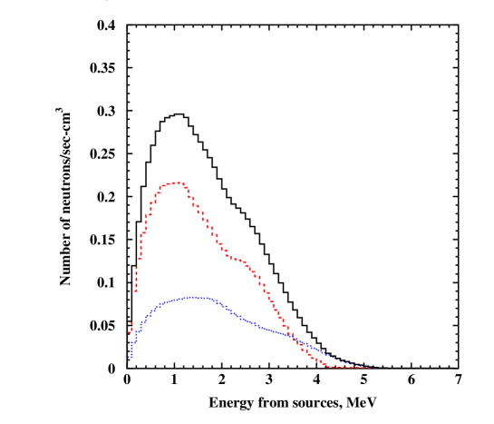
Figure 16: Energy spectra of neutrons calculated with modified SOURCES. Spectra due to contamination of 10 ppb of U (dashed histogram, middle) and 10 ppb of Th (dotted histogram, bottom) are shown. Solid histogram shows the total neutron production rate due to 10 ppb of U and Th in NaCl.

The Monte Carlo simulations were carried out in several stages, using GEANT4. For the first stage, neutrons generated via spontaneous fission and ($\alpha$,n) reactions from ²³⁸U and ²³²Th decay chains (calculated using the modified code SOURCES [16, 17]), were propagated to the rock-laboratory boundary and their parameters (such as energy, neutron position and the 3-momentum) were recorded. Figure 16 shows the spectra of neutrons from 10 ppb of ²³⁸U and 10 ppb of ²³²Th, calculated using SOURCES. These were the input spectra for the first stage of the GEANT4 simulations. At the second stage, these neutrons were propagated from the rock-laboratory boundary to the outer surface of the shielding (castle made of Cu and Fe). At the next stage, neutrons were transported to the outer surface of the scintillator (neutron parameters were always recorded) and, finally, inside the sensitive volume of the detector where they produced proton recoils by elastic scattering in the scintillator. The same procedure was applied to neutrons from the ²⁵²Cf source, starting from neutron propagation from Cf source to the shielding.

As a result of the simulations the absolute rate and energy spectra of neutrons at different surfaces and those of proton recoils in the detector were obtained. The simulated proton recoil rate from ²⁵²Cf source placed at a distance of 1 m away from the detector (same position as in the calibration run) was 14.51 s$\ {}^{-1}$ at 50-500 keV. Typical statistical error for all simulation results is less than 1%. This is much less than the experimental statistical and systematic uncertainties and will be neglected further on. The corresponding proton recoil rates from 10 ppb U and 10 ppb Th were found to be 4.22 d^-1 and 2.18 d^-1, respectively.

The efficiency of detecting delayed coincidences was calculated as the ratio of the measured rate (delayed coincidences with 100 keV threshold for the 2nd pulse) from Cf source to the calculated rate of single proton recoils at 50-500 keV and was found to be 0.037 $\pm$ 0.003. An efficiency of 0.036 $\pm$ 0.004 was obtained when the measured rates of delayed coincidences and the measured rate of single pulses (mainly proton recoils) were used, in agreement with the value obtained from simulation of proton recoils. (Note that good agreement was found between the measured and simulated rates and spectra of proton recoils from the Cf source, as shown in Figure 6 and discussed in Section 3). The same efficiency was then used to convert the calculated rate of proton recoils from background neutrons into the expected rate of delayed coincidences.

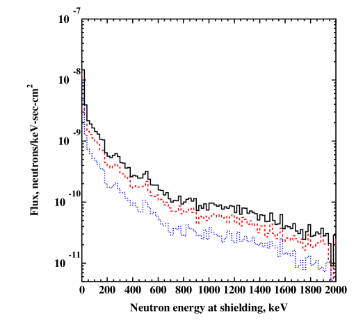
Figure 17: Energy spectra of neutrons at the outer surface of the shielding due to contamination of 10 ppb U (dashed histogram, middle) and 10 ppb Th (dotted histogram, bottom), calculated using GEANT4. The total background (the sum of U and Th contributions) is shown with the solid histogram.

The simulated fluxes of neutrons at the outer surface of the shielding, from 10 ppb U, 10 ppb Th and the sum, are shown in Figure 17. The energy spectra of proton recoils from GEANT4 simulations of U/Th background (the sum of the contributions from the two isotopes) and ²⁵²Cf are compared in Figure 18. The relative normalisation is done in order to have similar flux at about 50 keV and to compare the shapes of the two spectra. Figure 19 depicts the simulated fluxes of neutrons from the background and Cf source at the outer surface of the scintillator, which produced the proton recoil spectra shown in Figure  18. The spectrum from Cf was normalised to the overall area of the spectrum from the background. The shapes of the two spectra are quite similar with an estimated difference in total rate of 11% in the energy range of 0.4-1 MeV. Neutrons from this region contribute the most to the proton recoils at 50-500 keV and also are more likely to be captured in the scintillator. We used this difference of 11% as an estimate of systematic uncertainty from this method of efficiency calculation (see Section 5 for discussion on systematic uncertainties).

5 Results

In this Section, the results from the above studies are presented. In addition, all the efficiencies and uncertainties, which are taken into account in the final results, are discussed.

To investigate the effect of the dead time of DAQ on the rate of delayed coincidences in the background run, another short background run in which single pulses were recorded was carried out. From this run the rate of single pulses was obtained and the expected rate of random coincidences for the background run with two pulses recorded above 50 keV was calculated as $20.57\pm 0.36$ events per day. This is in good agreement with the measured rate of $23.02\pm 0.78$ events per day (the flat component in the time delay distribution similar to that shown in Figure 15 but without cuts, except the energy threshold of 50 keV for both pulses in an event). This demonstrates that the dead time does not affect the background measurements.

To evaluate the neutron flux, the trigger efficiency and the efficiencies of the various selection criteria should be taken into account. The energy dependent trigger efficiency can be calculated from the energy spectrum of events from ²⁵²Cf (single events without delayed coincidences) taken with two different energy thresholds, the threshold used in the experiment and another one half of this (5 mV). The ratio of events for specific energy gives the energy dependent trigger efficiency for the measurements with the higher threshold. It was found that the efficiency is 100% for energies more than 50 keV, the spectra measured with the two thresholds being practically identical above 50 keV. Note that the hardware energy threshold was set at about 20 keV, 2 photoelectrons from each PMT.

As mentioned before, the ratio of the observed charge in the tail of the pulse to the total charge was used to reject the correlated background from Bi$\rightarrow$Po$\rightarrow$Pb decay. The efficiency of this cut was calculated using data from a neutron calibration run with the ²⁵²Cf source with a software threshold of 50 keV for which the trigger efficiency is 100%. The fraction of events from ²⁵²Cf which passed the cut above the software threshold of 50 keV yields an efficiency of (61 $\pm$ 1)%. The value was obtained using fits to the time delay distributions similar to those shown in Figure 4. Taking into account this cut efficiency, the efficiency of detecting delayed coincidences discussed in Section 4 was reduced to 0.023$\pm$0.002.

Table 1 shows a summary of all the measured and predicted rates of proton recoils and coincidences from ²⁵²Cf and the backgound runs. Also the efficiency of detecting coincidences is shown, taking into account the efficiency of the tail/total cut.

The simulated energy spectrum of neutrons at the outer surface of shielding which produced proton recoils in the detector (within 50-500 keV energy range), as shown in Figure 20, indicates a threshold of 0.5 MeV for the measured neutron flux. The features seen in Figure 20 are not statistical but reflect the structures in the cross-section of neutron scattering on Na in the rock. The threshold at the rock-laboratory boundary is the same, since for most neutrons recorded at the surface of the shielding no interactions take place between the surface of the rock and the surface of the shielding.

Assuming 10 ppb U and 10 ppb Th, the neutron flux at the rock-laboratory boundary was calculated as $9.11\times 10^{-8}$ cm^-2 s^-1 above 0.5 MeV. This flux corresponds to neutrons which enter the laboratory hall for the first time, so does not take into account further scattering of neutrons from the walls. When this effect is included (neutrons which cross the cavern and scatter back from the rock into the cavern again), the flux at shielding is found to be $1.37\times 10^{-7}$ cm^-2 s^-1 above 0.5 MeV. This is 51% higher than the value at the rock-laboratory boundary, in agreement with Lemrani et al. [1], who claimed a 50% increment to the flux above 1 MeV due to the contribution of the back-scattered neutrons. For this flux a rate of 6.40 d^-1 for proton recoils at 50-500 keV was obtained. Taking into account the efficiency of detecting delayed coincidences of $0.023\pm 0.002$ we get a predicted rate of events in the background run of $0.147\pm 0.013$ per day. As the detector in fact measured a rate of $1.82\pm 0.64$ per day, the neutron flux was $(1.70\pm 0.60)\times 10^{-6}$ cm^-2 s^-1 above 0.5 MeV at shielding, and $(1.13\pm 0.40)\times 10^{-6}$ cm^-2 s^-1 above 0.5 MeV at the entrance to the cavern (no back scattering). An increase in the event rate of 1% is predicted by the simulations if proton recoils are considered without an upper energy cut of 0.5 MeV. Correcting for this increase we obtain the final neutron flux as $(1.72\pm 0.61)\times 10^{-6}$ cm^-2 s^-1 above 0.5 MeV at shielding, and $(1.14\pm 0.40)\times 10^{-6}$ cm^-2 s^-1 above 0.5 MeV at the entrance to the cavern. This result was obtained assuming equal concentrations of U and Th in rock. As the expected neutron spectra from U and Th after propagation in rock and shielding are very similar (see Figure 17) and the spectra of proton recoils produced by these neutrons are also similar, different assumptions about the relative fractions of U and Th result in very similar values for neutron flux, the difference being of the order of a few percent. Our measured neutron flux $(1.72\pm 0.61)\times 10^{-6}$ cm^-2 s^-1 above 0.5 MeV agrees well with the simulation result $1.21\times 10^{-6}$ cm^-2 s^-1 assuming measured concentrations of 67 ppb of U and 127 ppb of Th [8].

The same re-scaling, as was used to derive the neutron flux, should be applied to the original concentrations of U and Th resulting in $127\pm 45$ ppb of U and Th assuming their equal concentrations. If we assume that Th is twice as abundant as U, as measured by Smith et al. [8], then the resulting concentrations are $95\pm 34$ ppb of U and $190\pm 69$ ppb of Th. These values agree within errors with the recent measurements of the U and Th concentrations at Boulby [8]. They are also consistent with most of the previous measurements of the U and Th concentrations in Boulby rock using different techniques keeping in mind the large spread of the measured values [18]. Table 2 summarises the calculated and measured fluxes of neutrons at different surfaces, with different concentrations of U and Th.

The errors given above are purely statistical, determined by the fit to the measured time delay distribution. In addition to the statistical errors we can estimate systematic uncertainties. These are associated with the following parameters used to evaluate the neutron flux: (i) conversion of the charge to the energy scale for proton recoils; (ii) estimation of efficiencies; (iii) accuracy of simulations.

The uncertainty in the measured energy of proton recoils has two contributions: possible error and stability of the energy calibration using ⁶⁰Co and ¹³⁷Cs sources and uncertainty in the quenching factor for proton recoils.

A 5% change in the charge-to-energy conversion factor or in the width (standard deviation or $\sigma$) of the gaussian function for the energy resolution, changes significantly the calculated spectra of events from gamma sources, so the agreement with measurements seen in Figure 3 disappears. The uncertainty in the quenching factor for proton recoils is more difficult to estimate. There is, however, a way to estimate the possible error due to the two factors together (charge-to-energy conversion and quenching factor). As was mentioned before, in Figure 7, we observe an alpha peak in the correlated background at 0.8 MeV, but according to the quenching of alphas [19] the peak should be at about 0.96 MeV. This 20% difference in the peak position can be used as an estimate of the uncertainty in the energy scale for proton recoils. Changing the software energy threshold by 20% from 50 keV to 60 keV results in a decrease of the measured rate from ²⁵²Cf giving a possible error in the flux intensity of 10%. This exceeds significantly the estimated uncertainty in the charge-to-energy conversion factor and energy resolution (5%).

One of the uncertainties in the efficiency estimate comes from the statistical error of the fit to the time delay distribution for the calibration run with the Cf source. This error is of the order of 8%. Another uncertainty in the efficiency comes from the difference between the shape of the flux of neutrons from the ²⁵²Cf source and background, at the outer surface of the scintillator, as shown in Figure 19, which was calculated in Section 4 as 11%.

The simulations directly affect the neutron flux evaluated from the measured rate through the charge-to-energy conversion, proton recoil detection efficiency (including quenching), simulated energy resolution and other effects. In fact the accuracy of simulations has partly been considered when the corresponding effects have been studied (see above). The measured and predicted proton recoil rates from the neutron source agree within 14%. The small difference arises from the presence of gammas from neutron captures in the data and their absence in the simulations. We estimate then the uncertainty due to simulations as 14%. The total systematic uncertainty can be found by adding the four errors discussed above in quadrature resulting in a value of 22%. A summary of all the systematic uncertainties is shown in Table 3.

6 Conclusions

A technique to measure low intensity neutron flux has been developed based on a detection of delayed coincidences between proton recoils and neutron capture gammas. The neutron flux in the Boulby Underground Laboratory at a depth of 2800 m w.e. was measured using liquid scintillator detector as $(1.72\pm 0.61(stat.)\pm 0.38(syst.))\times 10^{-6}$ cm^-2 s^-1 above 0.5 MeV including the effect of neutron back-scattering from the cavern walls. This flux corresponds to the concentrations of either$\ 127\pm 45(stat.)\pm 28(syst.)$ ppb of U and Th, assuming their concentrations are equal or $95\pm 34(stat.)\pm 21(syst.)$ ppb of U and $190\pm 69(stat.)\pm 42(syst.)$ ppb of Th, if Th is twice as abundant as U.

7 Acknowledgments

This work has been supported by the ILIAS integrating activity (Contract No. RII3-CT-2004-506222) as part of the EU FP6 programme in Astroparticle Physics. We aknowledge the financial support from the Particle Physics and Astronomy Research Council (PPARC). We also like to thank the Cleveland Potash Ltd for assistance.

Table 1: Measured and predicted rates of single proton recoils and delayed coincidences from the ²⁵²Cf and the backgound runs. Rows 1 and 2 show the calculated and the measured rate of single proton recoils without delayed coincidences from ²⁵²Cf source on top of the castle. In rows 3 and 4, the measured rate of delayed coincidences and the efficiency of detecting delayed coincidences, calculated from the measured values, are shown respectively. In rows 5-7 similar rates and efficiency are shown for ²⁵²Cf source at a distance of 1 m away from the detector. No run with single proton recoil measurements, with a source at a distance of 1 m from the detector, was performed before the neutron shielding was installed around the detector. In this case the efficiency is calculated from the calculated rate of single proton recoils and the measured rate of delayed coincidences. The last row shows the measured rate of delayed coincidences for the background run. In the efficiency calculation, the efficiency of the tail/total cut was taken into account (see Section 5).

	Calculated rate of single proton recoils, s-1	140.30
252Cf source on top	Measured rate of single proton recoils, s-1	163.88 $\pm$ 1.40
of the castle	Measured rate of delayed coincidences, s-1	5.87 $\pm$ 0.68
	Efficiency of detecting delayed coincidences	0.022 $\pm$ 0.002
252Cf source 1 m away	Calculated rate of single proton recoils, s-1	14.51
from the detector	Measured rate of delayed coincidences, s-1	0.53 $\pm$ 0.04
	Efficiency of detecting delayed coincidences	0.023 $\pm$ 0.002
Background run	Measured rate of delayed coincidences, d-1	1.82 $\pm$ 0.64

Table 2: Flux of neutrons at different surfaces with different concentrations of U and Th. The first column shows the concentrations of U and Th in rock. At the beginning, they were assumed to be 10 ppb U and 10 ppb Th (rows 1-4). Later, the real concentrations of U and Th were found from the data analysis (rows 5-6), assuming equal concentration of U and Th. The second column shows the surface on which the flux was calculated, for different concentration of U, Th and the last column shows the corresponding fluxes. The errors given for the measured concentrations and fluxes are statistical.

Concentration in rock	Surface	Flux above 0.5 MeV
		[cm-2 s-1]
		Simulated Flux
10ppb U	Rock w/o back scattering	$6.02\times 10^{-8}$
10ppb Th	Rock w/o back scattering	$3.09\times 10^{-8}$
10ppb U	Outer surface of shielding	$9.06\times 10^{-8}$
10ppb Th	Outer surface of shielding	$4.66\times 10^{-8}$
		Measured Flux
(127 $\pm$ 45) ppb U and Th	Rock w/o back scattering	$(1.14\pm 0.40)\times 10^{-6}$
(127 $\pm$ 45) ppb U and Th	Outer surface of shielding	$(1.72\pm 0.61)\times 10^{-6}$

Table 3: Systematic uncertainties.

Sources of systematic uncertainties	Relative
	systematic
	uncertainties
Charge to energy conversion and quenching factor	0.10
Fit to the time delay distribution for 252Cf run	0.08
Difference between neutron spectra from 252Cf source and background	0.11
Difference between measured and simulated recoil rates	0.14
Total systematic uncertainty	0.22

Figure 2: The functional diagram of the electronics for neutron measurement and neutron calibration (2 pulses in delayed coincidences). The discriminators are labeled as ’D’, the coincidence units as ’C.U.’ and the timers as ’T’.

Figure 9: The rate of the correlated background as a function of time for the first month after the installation of the detector underground. These data were not included in the analysis of neutron flux.

$\begin{array}[]{c@{\hspace{5mm}}c}\includegraphics[width=199.16928pt]{correlbg_041110_ratio1.ps}\hfil\hskip 14.22636pt&\includegraphics[width=199.16928pt]{correlbg_041110_ratio.ps}\\ \hskip 28.45274pt\mbox{\small{(a)}}\hfil\hskip 14.22636pt&\mbox{\small{(b)}}\end{array}$

Figure 10: The ratio of charge in the tail of the pulse to the total charge for the first (a) and second (b) pulses for the correlated background events (Bi$\rightarrow$Po$\rightarrow$Pb decay).

$\begin{array}[]{c@{\hspace{5mm}}c}\includegraphics[width=199.16928pt]{ntfiles126_191205bw5_ratio1p_beforecuts.ps}\hfil\hskip 14.22636pt&\includegraphics[width=199.16928pt]{ntfiles126_191205bw5_ratio2p_beforecuts.ps}\\ \hskip 28.45274pt\mbox{\small{(a)}}\hfil\hskip 14.22636pt&\mbox{\small{(b)}}\end{array}$

Figure 13: The ratio of charge in the tail of the pulse to the total charge for the first (a) and the second (b) pulses in the events included in the analysis of neutron flux, prior to the applied cuts.

$\begin{array}[]{c@{\hspace{5mm}}c}\includegraphics[width=199.16928pt]{ntfiles126_191205bw5_ratio1p.ps}\hfil\hskip 14.22636pt&\includegraphics[width=199.16928pt]{ntfiles126_191205bw5_ratio2p.ps}\\ \hskip 28.45274pt\mbox{\small{(a)}}\hfil\hskip 14.22636pt&\mbox{\small{(b)}}\end{array}$

Figure 14: The ratio of charge in the tail of the pulse to the total charge for the first (a) and the second (b) pulses in the events included in the analysis of neutron flux, after the applied cuts.

$\begin{array}[]{c@{\hspace{5mm}}c}\includegraphics[width=199.16928pt]{tdelay_126f_005-05e1.ps}\hfil\hskip 14.22636pt&\includegraphics[width=199.16928pt]{shieldedfitline.ps}\\ \hskip 28.45274pt\mbox{\small{(a)}}\hfil\hskip 14.22636pt&\mbox{\small{(b)}}\end{array}$

Figure 15: Time delay distributions for the run without neutron shielding (a) and for the run with polypropylene shielding (b). The solid curve in (a) is the fit with a two-component function, described in the text, with fixed mean time delay. The solid curve in (b) is the fit assuming a flat background only. Both graphs include first pulses with measured energy of 50-500 keV and second pulses with energy greater than 100 keV.

Figure 18: Energy spectra of proton recoils due to background (U and Th, dashed histogram) and due to Cf neutrons (solid histogram), calculated using GEANT4. Cf spectrum was normalised to the background spectrum at 50 keV.

Figure 19: Flux of neutrons, which produced proton recoils, from the background (dashed histogram) and the Cf source (solid histogram), at the outer surface of the scintillator, calculated using GEANT4. The spectrum of Cf was normalised to the integrated spectrum of the background (total fluxes above 0.4 MeV are assumed to be the same).

Figure 20: Energy spectrum of neutrons (due to 100 ppb U and Th) at the outer surface of the shielding, which produce proton recoils with measured energy 50-500 keV. The spectrum was simulated using GEANT4. A threshold of 0.5 MeV for the measured neutron flux was estimated from this graph.

References

- [1] R. Lemrani et al., Nuclear Instruments and Methods A, 560 (2006), 454.
- [2] H. Wulandari et al., Astroparticle Physics, 22 (2004) 313-322.
- [3] M. Robinson et al., Nuclear Instruments and Methods A 511 (2003) 347.
- [4] G. J. Alner et al., Physics Letter B, 616 (2005) 17-24.
- [5] G. J. Alner et al., Nuclear Instruments and Methods A 555 (2005) 173-183.
- [6] G. J. Alner et al., Astroparticle Physics, 23 (2005) 444-462.
- [7] G. J. Alner et al., New Astronomy Reviews 49 (2005) 259-263.
- [8] P. F. Smith et al., Astroparticle Physics 22 (2005) 409.
- [9] P. K. Lightfoot et al., Nuclear Instruments and Methods A 522 (2004) 430-466.
- [10] S. Agostinelli et al., GEANT4 Collaboration, Nuclear Instruments and Methods A 506 (2003) 250.
- [11] J. B. Birks, Theory And Practice of Scintillation Counting, Pergamon Press (1664) 383.
- [12] M. Anghinolfi et al., Nuclear Instruments and Methods A 165 (1979) 217-224.
- [13] Briesmeister (Ed.) et al. MCNP - Version 4B (and later), LA-12625-M, LANL (1997).
- [14] http://mcnpx.lanl.gov.
- [15] GEANT3 Collaboration. CERN-DD/EE/84-1, September 1987.
- [16] W. B. Wilson et al., SOURCES-4C: A Code for Calculating (alpa,n) Spontaneous Fission and Delayed Neutron Sources and Spectra, American Nuclei Society/Radiation Protection and Shielding Division (2002).
- [17] M. J. Carson et al., Astroparticle Physics 21 (2004) 667.
- [18] http://hepwww.rl.ac.uk/ukdmc/Radioactivity/uk.html.
- [19] V. V. Verbinski et al., Nuclear Instruments and Methods A 65 (1968) 8-25.