V.M. Abazov,35
B. Abbott,75
M. Abolins,65
B.S. Acharya,28
M. Adams,51
T. Adams,49
E. Aguilo,5
S.H. Ahn,30
M. Ahsan,59
G.D. Alexeev,35
G. Alkhazov,39
A. Alton,64,∗
G. Alverson,63
G.A. Alves,2
M. Anastasoaie,34
L.S. Ancu,34
T. Andeen,53
S. Anderson,45
B. Andrieu,16
M.S. Anzelc,53
Y. Arnoud,13
M. Arov,52
A. Askew,49
B. Åsman,40
A.C.S. Assis Jesus,3
O. Atramentov,49
C. Autermann,20
C. Avila,7
C. Ay,23
F. Badaud,12
A. Baden,61
L. Bagby,52
B. Baldin,50
D.V. Bandurin,59
P. Banerjee,28
S. Banerjee,28
E. Barberis,63
P. Bargassa,80
P. Baringer,58
C. Barnes,43
J. Barreto,2
J.F. Bartlett,50
U. Bassler,16
D. Bauer,43
S. Beale,5
A. Bean,58
M. Begalli,3
M. Begel,71
C. Belanger-Champagne,40
L. Bellantoni,50
A. Bellavance,67
J.A. Benitez,65
S.B. Beri,26
G. Bernardi,16
R. Bernhard,22
L. Berntzon,14
I. Bertram,42
M. Besançon,17
R. Beuselinck,43
V.A. Bezzubov,38
P.C. Bhat,50
V. Bhatnagar,26
M. Binder,24
C. Biscarat,19
I. Blackler,43
G. Blazey,52
F. Blekman,43
S. Blessing,49
D. Bloch,18
K. Bloom,67
A. Boehnlein,50
D. Boline,62
T.A. Bolton,59
G. Borissov,42
K. Bos,33
T. Bose,77
A. Brandt,78
R. Brock,65
G. Brooijmans,70
A. Bross,50
D. Brown,78
N.J. Buchanan,49
D. Buchholz,53
M. Buehler,81
V. Buescher,22
S. Burdin,50
S. Burke,45
T.H. Burnett,82
E. Busato,16
C.P. Buszello,43
J.M. Butler,62
P. Calfayan,24
S. Calvet,14
J. Cammin,71
S. Caron,33
W. Carvalho,3
B.C.K. Casey,77
N.M. Cason,55
H. Castilla-Valdez,32
S. Chakrabarti,17
D. Chakraborty,52
K.M. Chan,71
A. Chandra,48
F. Charles,18
E. Cheu,45
F. Chevallier,13
D.K. Cho,62
S. Choi,31
B. Choudhary,27
L. Christofek,77
D. Claes,67
B. Clément,18
C. Clément,40
Y. Coadou,5
M. Cooke,80
W.E. Cooper,50
M. Corcoran,80
F. Couderc,17
M.-C. Cousinou,14
B. Cox,44
S. Crépé-Renaudin,13
D. Cutts,77
M. Ćwiok,29
H. da Motta,2
A. Das,62
M. Das,60
B. Davies,42
G. Davies,43
K. De,78
P. de Jong,33
S.J. de Jong,34
E. De La Cruz-Burelo,64
C. De Oliveira Martins,3
J.D. Degenhardt,64
F. Déliot,17
M. Demarteau,50
R. Demina,71
D. Denisov,50
S.P. Denisov,38
S. Desai,50
H.T. Diehl,50
M. Diesburg,50
M. Doidge,42
A. Dominguez,67
H. Dong,72
L.V. Dudko,37
L. Duflot,15
S.R. Dugad,28
D. Duggan,49
A. Duperrin,14
J. Dyer,65
A. Dyshkant,52
M. Eads,67
D. Edmunds,65
J. Ellison,48
V.D. Elvira,50
Y. Enari,77
S. Eno,61
P. Ermolov,37
H. Evans,54
A. Evdokimov,36
V.N. Evdokimov,38
L. Feligioni,62
A.V. Ferapontov,59
T. Ferbel,71
F. Fiedler,24
F. Filthaut,34
W. Fisher,50
H.E. Fisk,50
M. Ford,44
M. Fortner,52
H. Fox,22
S. Fu,50
S. Fuess,50
T. Gadfort,82
C.F. Galea,34
E. Gallas,50
E. Galyaev,55
C. Garcia,71
A. Garcia-Bellido,82
V. Gavrilov,36
A. Gay,18
P. Gay,12
W. Geist,18
D. Gelé,18
R. Gelhaus,48
C.E. Gerber,51
Y. Gershtein,49
D. Gillberg,5
G. Ginther,71
N. Gollub,40
B. Gómez,7
A. Goussiou,55
P.D. Grannis,72
H. Greenlee,50
Z.D. Greenwood,60
E.M. Gregores,4
G. Grenier,19
Ph. Gris,12
J.-F. Grivaz,15
A. Grohsjean,24
S. Grünendahl,50
M.W. Grünewald,29
F. Guo,72
J. Guo,72
G. Gutierrez,50
P. Gutierrez,75
A. Haas,70
N.J. Hadley,61
P. Haefner,24
S. Hagopian,49
J. Haley,68
I. Hall,75
R.E. Hall,47
L. Han,6
K. Hanagaki,50
P. Hansson,40
K. Harder,44
A. Harel,71
R. Harrington,63
J.M. Hauptman,57
R. Hauser,65
J. Hays,43
T. Hebbeker,20
D. Hedin,52
J.G. Hegeman,33
J.M. Heinmiller,51
A.P. Heinson,48
U. Heintz,62
C. Hensel,58
K. Herner,72
G. Hesketh,63
M.D. Hildreth,55
R. Hirosky,81
J.D. Hobbs,72
B. Hoeneisen,11
H. Hoeth,25
M. Hohlfeld,15
S.J. Hong,30
R. Hooper,77
P. Houben,33
Y. Hu,72
Z. Hubacek,9
V. Hynek,8
I. Iashvili,69
R. Illingworth,50
A.S. Ito,50
S. Jabeen,62
M. Jaffré,15
S. Jain,75
K. Jakobs,22
C. Jarvis,61
A. Jenkins,43
R. Jesik,43
K. Johns,45
C. Johnson,70
M. Johnson,50
A. Jonckheere,50
P. Jonsson,43
A. Juste,50
D. Käfer,20
S. Kahn,73
E. Kajfasz,14
A.M. Kalinin,35
J.M. Kalk,60
J.R. Kalk,65
S. Kappler,20
D. Karmanov,37
J. Kasper,62
P. Kasper,50
I. Katsanos,70
D. Kau,49
R. Kaur,26
R. Kehoe,79
S. Kermiche,14
N. Khalatyan,62
A. Khanov,76
A. Kharchilava,69
Y.M. Kharzheev,35
D. Khatidze,70
H. Kim,31
T.J. Kim,30
M.H. Kirby,34
B. Klima,50
J.M. Kohli,26
J.-P. Konrath,22
M. Kopal,75
V.M. Korablev,38
J. Kotcher,73
B. Kothari,70
A. Koubarovsky,37
A.V. Kozelov,38
D. Krop,54
A. Kryemadhi,81
T. Kuhl,23
A. Kumar,69
S. Kunori,61
A. Kupco,10
T. Kurča,19
J. Kvita,8
D. Lam,55
S. Lammers,70
G. Landsberg,77
J. Lazoflores,49
A.-C. Le Bihan,18
P. Lebrun,19
W.M. Lee,50
A. Leflat,37
F. Lehner,41
V. Lesne,12
J. Leveque,45
P. Lewis,43
J. Li,78
L. Li,48
Q.Z. Li,50
S.M. Lietti,4
J.G.R. Lima,52
D. Lincoln,50
J. Linnemann,65
V.V. Lipaev,38
R. Lipton,50
Z. Liu,5
L. Lobo,43
A. Lobodenko,39
M. Lokajicek,10
A. Lounis,18
P. Love,42
H.J. Lubatti,82
M. Lynker,55
A.L. Lyon,50
A.K.A. Maciel,2
R.J. Madaras,46
P. Mättig,25
C. Magass,20
A. Magerkurth,64
N. Makovec,15
P.K. Mal,55
H.B. Malbouisson,3
S. Malik,67
V.L. Malyshev,35
H.S. Mao,50
Y. Maravin,59
R. McCarthy,72
A. Melnitchouk,66
A. Mendes,14
L. Mendoza,7
P.G. Mercadante,4
M. Merkin,37
K.W. Merritt,50
A. Meyer,20
J. Meyer,21
M. Michaut,17
H. Miettinen,80
T. Millet,19
J. Mitrevski,70
J. Molina,3
R.K. Mommsen,44
N.K. Mondal,28
J. Monk,44
R.W. Moore,5
T. Moulik,58
G.S. Muanza,19
M. Mulders,50
M. Mulhearn,70
O. Mundal,22
L. Mundim,3
E. Nagy,14
M. Naimuddin,27
M. Narain,62
N.A. Naumann,34
H.A. Neal,64
J.P. Negret,7
P. Neustroev,39
C. Noeding,22
A. Nomerotski,50
S.F. Novaes,4
T. Nunnemann,24
V. O’Dell,50
D.C. O’Neil,5
G. Obrant,39
C. Ochando,15
V. Oguri,3
N. Oliveira,3
D. Onoprienko,59
N. Oshima,50
J. Osta,55
R. Otec,9
G.J. Otero y Garzón,51
M. Owen,44
P. Padley,80
M. Pangilinan,62
N. Parashar,56
S.-J. Park,71
S.K. Park,30
J. Parsons,70
R. Partridge,77
N. Parua,72
A. Patwa,73
G. Pawloski,80
P.M. Perea,48
K. Peters,44
Y. Peters,25
P. Pétroff,15
M. Petteni,43
R. Piegaia,1
J. Piper,65
M.-A. Pleier,21
P.L.M. Podesta-Lerma,32
V.M. Podstavkov,50
Y. Pogorelov,55
M.-E. Pol,2
A. Pompoš,75
B.G. Pope,65
A.V. Popov,38
C. Potter,5
W.L. Prado da Silva,3
H.B. Prosper,49
S. Protopopescu,73
J. Qian,64
A. Quadt,21
B. Quinn,66
M.S. Rangel,2
K.J. Rani,28
K. Ranjan,27
P.N. Ratoff,42
P. Renkel,79
S. Reucroft,63
M. Rijssenbeek,72
I. Ripp-Baudot,18
F. Rizatdinova,76
S. Robinson,43
R.F. Rodrigues,3
C. Royon,17
P. Rubinov,50
R. Ruchti,55
G. Sajot,13
A. Sánchez-Hernández,32
M.P. Sanders,16
A. Santoro,3
G. Savage,50
L. Sawyer,60
T. Scanlon,43
D. Schaile,24
R.D. Schamberger,72
Y. Scheglov,39
H. Schellman,53
P. Schieferdecker,24
C. Schmitt,25
C. Schwanenberger,44
A. Schwartzman,68
R. Schwienhorst,65
J. Sekaric,49
S. Sengupta,49
H. Severini,75
E. Shabalina,51
M. Shamim,59
V. Shary,17
A.A. Shchukin,38
R.K. Shivpuri,27
D. Shpakov,50
V. Siccardi,18
R.A. Sidwell,59
V. Simak,9
V. Sirotenko,50
P. Skubic,75
P. Slattery,71
R.P. Smith,50
G.R. Snow,67
J. Snow,74
S. Snyder,73
S. Söldner-Rembold,44
X. Song,52
L. Sonnenschein,16
A. Sopczak,42
M. Sosebee,78
K. Soustruznik,8
M. Souza,2
B. Spurlock,78
J. Stark,13
J. Steele,60
V. Stolin,36
A. Stone,51
D.A. Stoyanova,38
J. Strandberg,64
S. Strandberg,40
M.A. Strang,69
M. Strauss,75
R. Ströhmer,24
D. Strom,53
M. Strovink,46
L. Stutte,50
S. Sumowidagdo,49
P. Svoisky,55
A. Sznajder,3
M. Talby,14
P. Tamburello,45
W. Taylor,5
P. Telford,44
J. Temple,45
B. Tiller,24
M. Titov,22
V.V. Tokmenin,35
M. Tomoto,50
T. Toole,61
I. Torchiani,22
T. Trefzger,23
S. Trincaz-Duvoid,16
D. Tsybychev,72
B. Tuchming,17
C. Tully,68
P.M. Tuts,70
R. Unalan,65
L. Uvarov,39
S. Uvarov,39
S. Uzunyan,52
B. Vachon,5
P.J. van den Berg,33
B. van Eijk,35
R. Van Kooten,54
W.M. van Leeuwen,33
N. Varelas,51
E.W. Varnes,45
A. Vartapetian,78
I.A. Vasilyev,38
M. Vaupel,25
P. Verdier,19
L.S. Vertogradov,35
M. Verzocchi,50
F. Villeneuve-Seguier,43
P. Vint,43
J.-R. Vlimant,16
E. Von Toerne,59
M. Voutilainen,67,†
M. Vreeswijk,33
H.D. Wahl,49
L. Wang,61
M.H.L.S Wang,50
J. Warchol,55
G. Watts,82
M. Wayne,55
G. Weber,23
M. Weber,50
H. Weerts,65
N. Wermes,21
M. Wetstein,61
A. White,78
D. Wicke,25
G.W. Wilson,58
S.J. Wimpenny,48
M. Wobisch,50
J. Womersley,50
D.R. Wood,63
T.R. Wyatt,44
Y. Xie,77
S. Yacoob,53
R. Yamada,50
M. Yan,61
T. Yasuda,50
Y.A. Yatsunenko,35
K. Yip,73
H.D. Yoo,77
S.W. Youn,53
C. Yu,13
J. Yu,78
A. Yurkewicz,72
A. Zatserklyaniy,52
C. Zeitnitz,25
D. Zhang,50
T. Zhao,82
B. Zhou,64
J. Zhu,72
M. Zielinski,71
D. Zieminska,54
A. Zieminski,54
V. Zutshi,52
and E.G. Zverev37 (DØ Collaboration) 1Universidad de Buenos Aires, Buenos Aires, Argentina 2LAFEX, Centro Brasileiro de Pesquisas Físicas,
Rio de Janeiro, Brazil 3Universidade do Estado do Rio de Janeiro,
Rio de Janeiro, Brazil 4Instituto de Física Teórica, Universidade
Estadual Paulista, São Paulo, Brazil 5University of Alberta, Edmonton, Alberta, Canada,
Simon Fraser University, Burnaby, British Columbia, Canada, York University, Toronto, Ontario, Canada, and
McGill University, Montreal, Quebec, Canada 6University of Science and Technology of China, Hefei,
People’s Republic of China 7Universidad de los Andes, Bogotá, Colombia 8Center for Particle Physics, Charles University,
Prague, Czech Republic 9Czech Technical University, Prague, Czech Republic 10Center for Particle Physics, Institute of Physics,
Academy of Sciences of the Czech Republic,
Prague, Czech Republic 11Universidad San Francisco de Quito, Quito, Ecuador 12Laboratoire de Physique Corpusculaire, IN2P3-CNRS,
Université Blaise Pascal, Clermont-Ferrand, France 13Laboratoire de Physique Subatomique et de Cosmologie,
IN2P3-CNRS, Universite de Grenoble 1, Grenoble, France 14CPPM, IN2P3-CNRS, Université de la Méditerranée,
Marseille, France 15Laboratoire de l’Accélérateur Linéaire,
IN2P3-CNRS et Université Paris-Sud, Orsay, France 16LPNHE, IN2P3-CNRS, Universités Paris VI and VII,
Paris, France 17DAPNIA/Service de Physique des Particules, CEA, Saclay,
France 18IPHC, IN2P3-CNRS, Université Louis Pasteur, Strasbourg,
France, and Université de Haute Alsace,
Mulhouse, France 19Institut de Physique Nucléaire de Lyon, IN2P3-CNRS,
Université Claude Bernard, Villeurbanne, France 20III. Physikalisches Institut A, RWTH Aachen,
Aachen, Germany 21Physikalisches Institut, Universität Bonn,
Bonn, Germany 22Physikalisches Institut, Universität Freiburg,
Freiburg, Germany 23Institut für Physik, Universität Mainz,
Mainz, Germany 24Ludwig-Maximilians-Universität München,
München, Germany 25Fachbereich Physik, University of Wuppertal,
Wuppertal, Germany 26Panjab University, Chandigarh, India 27Delhi University, Delhi, India 28Tata Institute of Fundamental Research, Mumbai, India 29University College Dublin, Dublin, Ireland 30Korea Detector Laboratory, Korea University,
Seoul, Korea 31SungKyunKwan University, Suwon, Korea 32CINVESTAV, Mexico City, Mexico 33FOM-Institute NIKHEF and University of
Amsterdam/NIKHEF, Amsterdam, The Netherlands 34Radboud University Nijmegen/NIKHEF, Nijmegen, The
Netherlands 35Joint Institute for Nuclear Research, Dubna, Russia 36Institute for Theoretical and Experimental Physics,
Moscow, Russia 37Moscow State University, Moscow, Russia 38Institute for High Energy Physics, Protvino, Russia 39Petersburg Nuclear Physics Institute,
St. Petersburg, Russia 40Lund University, Lund, Sweden, Royal Institute of
Technology and Stockholm University, Stockholm,
Sweden, and Uppsala University, Uppsala, Sweden 41Physik Institut der Universität Zürich,
Zürich, Switzerland 42Lancaster University, Lancaster, United Kingdom 43Imperial College, London, United Kingdom 44University of Manchester, Manchester, United Kingdom 45University of Arizona, Tucson, Arizona 85721, USA 46Lawrence Berkeley National Laboratory and University of
California, Berkeley, California 94720, USA 47California State University, Fresno, California 93740, USA 48University of California, Riverside, California 92521, USA 49Florida State University, Tallahassee, Florida 32306, USA 50Fermi National Accelerator Laboratory,
Batavia, Illinois 60510, USA 51University of Illinois at Chicago,
Chicago, Illinois 60607, USA 52Northern Illinois University, DeKalb, Illinois 60115, USA 53Northwestern University, Evanston, Illinois 60208, USA 54Indiana University, Bloomington, Indiana 47405, USA 55University of Notre Dame, Notre Dame, Indiana 46556, USA 56Purdue University Calumet, Hammond, Indiana 46323, USA 57Iowa State University, Ames, Iowa 50011, USA 58University of Kansas, Lawrence, Kansas 66045, USA 59Kansas State University, Manhattan, Kansas 66506, USA 60Louisiana Tech University, Ruston, Louisiana 71272, USA 61University of Maryland, College Park, Maryland 20742, USA 62Boston University, Boston, Massachusetts 02215, USA 63Northeastern University, Boston, Massachusetts 02115, USA 64University of Michigan, Ann Arbor, Michigan 48109, USA 65Michigan State University,
East Lansing, Michigan 48824, USA 66University of Mississippi,
University, Mississippi 38677, USA 67University of Nebraska, Lincoln, Nebraska 68588, USA 68Princeton University, Princeton, New Jersey 08544, USA 69State University of New York, Buffalo, New York 14260, USA 70Columbia University, New York, New York 10027, USA 71University of Rochester, Rochester, New York 14627, USA 72State University of New York,
Stony Brook, New York 11794, USA 73Brookhaven National Laboratory, Upton, New York 11973, USA 74Langston University, Langston, Oklahoma 73050, USA 75University of Oklahoma, Norman, Oklahoma 73019, USA 76Oklahoma State University, Stillwater, Oklahoma 74078, USA 77Brown University, Providence, Rhode Island 02912, USA 78University of Texas, Arlington, Texas 76019, USA 79Southern Methodist University, Dallas, Texas 75275, USA 80Rice University, Houston, Texas 77005, USA 81University of Virginia, Charlottesville,
Virginia 22901, USA 82University of Washington, Seattle, Washington 98195, USA
(Dec 5, 2006)
Abstract
We search for the technicolor process in events containing one electron and two jets,
in data corresponding
to an integrated luminosity of 390 pb-1, recorded by
the D0 experiment at the Fermilab Tevatron.
Technicolor predicts that technipions, , decay dominantly into
, , or ,
depending on their charge.
In these events and quarks are identified by their
secondary decay vertices within jets.
Two analysis methods based on topological variables are presented.
Since no excess above the standard model prediction was found,
the result is presented as an exclusion in the vs. mass plane for
a given set of model parameters.
pacs:
12.60.Nz, 13.85.Rm
Technicolor (TC), first formulated by Weinberg and Susskind Wei1 ; Sus1 ,
provides a dynamical explanation of electroweak symmetry breaking through a
new strong gauge interaction acting on new fermions, called
“technifermions.” Technicolor is a non-Abelian gauge theory modeled after
Quantum Chromodynamics (QCD). In its low-energy limit, a spontaneous breaking
of the global chiral symmetry in the technifermion sector
leads to electroweak symmetry breaking. The
Nambu-Goldstone bosons produced in this process are called technipions,
, in analogy with the pions of QCD. Three of these technipions become
the longitudinal components of the and bosons, making them
massive.
An additional gauge interaction, called extended
technicolor etc1 ; etc2 , couples standard model fermions and
technifermions to provide a mechanism for generating quark and lepton masses. By
limiting the running of the technicolor coupling constant, walking
technicolor wtc avoids flavor-changing neutral currents.
To generate masses as large as the top quark mass,
another interaction, topcolor, seems to be necessary, thereby
giving rise to topcolor-assisted technicolor models tc2 .
Extensions of the basic technicolor model tend to require the
number of technifermion doublets to be large. In general, the
technicolor scale , where
is the technipion decay constant, depends inversely on the number of
technifermion doublets: .
For large , the lowest lying technihadrons have masses on the order of
few hundred GeV. This scenario is referred to as low-scale
technicolor Lane1 . Low-scale
technicolor models predict the existence of scalar technimesons, and
, and vector technimesons, and . General features
of low-scale technicolor have been summarized in the technicolor strawman
model (TCSM) Lane2 ; Lane4 . The analysis presented in this paper is based on Ref. Lane4 .
Vector technimesons are expected to be produced with
substantial rates at the Fermilab Tevatron Collider via the
Drell-Yan-like electroweak process
or . In walking technicolor, it is expected that vector
technimesons decay to a gauge boson (, , ) and a technipion or
to fermion-antifermion pairs. The production cross sections and branching
fractions depend on the masses of the vector technimesons, and
, on the technicolor-charges of the technifermions, on the
mass differences between the vector and scalar technimesons, which determine
the spectrum of accessible decay channels, and on two mass parameters,
for axial-vector and for vector couplings. The parameter controls
the rate for the decay and is
unknown a priori. Scaling from the QCD decay
, the authors of Ref. Lane4
suggest a value of several hundred GeV. We set , and
evaluate the production and decay rates at two different values: 100 and 500
GeV. For all other parameters, we use the default values quoted in Table III
of Ref. Lane4 .
Technipion coupling to the standard model
particles is proportional to their masses,
therefore technipions in the mass range
considered here predominantly decay into , , or
, depending on their charge.
In this Letter, we describe a search for the decay of vector technimesons to ,
followed by the decays and , , or
. In the D0 detector, which is described in detail in
Ref. d0det , the signature of this process is an isolated electron and
missing transverse momentum () from the undetected neutrino from the
decay of the boson, and two jets of hadrons coming from the fragmentation
of the quarks from the decay of the technipion. Jets are reconstructed
using the Run II cone algorithm cone with a cone size of 0.5.
We search for events with this signature in the data collected with a single electron
trigger until July 2004 and corresponding to
an integrated luminosity of 38825 pb-1oldlumi .
There are a number of standard model processes that can result in the same
final state signature as production. Vector boson production in association
with jets is the dominant background. boson production can be suppressed by
vetoing on a second electron and requiring significant . Most of
the jets in +jets events originate from the fragmentation of light quarks
or gluons and therefore requiring the explicit identification of at least one
jet from the fragmentation of a or quark suppresses most of this background,
leaving only , , , and events. Top quark
production followed by the decay to is another background.
Top-antitop quark pair production typically results in either an additional
lepton or a higher jet multiplicity from the decay of the second top quark,
and this background can be reduced by selecting events with exactly two jets. Single top
quark production is an irreducible background, but it has a smaller cross
section. We simulate all these processes using either pythiapythia or alpgenalpg Monte Carlo (MC) generators,
followed by the D0 detector simulation based on geantgeant .
Quark hadronization and fragmentation is
simulated using pythia.
The multijet background is due to events with
poorly measured jets, resulting in missing momentum and a jet that
is misidentified as an electron. Background from the mistagged +jets process originates
from events in which a light-quark or gluon jet is incorrectly identified as a
jet. These instrumental background contributions are estimated from the
same data sample before requiring the identification of a jet.
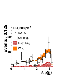
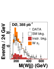
Figure 1: Distributions of , and after final kinematic selection. The signal is shown for GeV and GeV. Arrows at
the bottom indicate the cuts applied in the cut-based analysis for the signal mass point shown.
We select events in which there is exactly one well-identified electron based
on tracking and calorimeter data with transverse momentum GeV and
pseudorapidity pseudorapidity .
There must be significant , measured
in two ways: GeV computed as the negative sum of the jet
momentum vectors and the electron momentum vector and GeV which
also includes the calorimeter energy deposit not assigned to the electron or the
jets. We require the transverse mass GeV.
We further require the presence of exactly two jets
with GeV and .
To further reduce backgrounds, we take advantage of the long lifetime of flavored
hadrons. Tracks from the decay products of hadrons may not project back to
the proton-antiproton collision, but have a significant impact
parameter. They can therefore be identified and used to reconstruct the decay
vertex of the hadron. A jet is tagged as a jet if there is a secondary decay vertex within of the jet axis. We require at least one of the jets to be -tagged. This leaves us with 117 events in our final data sample.
The expected background event yields are listed in Table 1.
When estimating these yields, each Monte Carlo event is weighted by the probability
that at least one jet is tagged as a jet. The tagging probability is
parameterized as a function of jet flavor, jet , and . The
efficiency of tagging a jet from the fragmentation of a quark is derived
from collider data which were enriched in their jet contents by requiring
a muon to be reconstructed within at least one jet to preferentially select
jets with semileptonic decays. The probability of tagging a jet is
derived from the tagging probability for jets by multiplying by the ratio
of tagging probabilities for and jets derived from MC
simulations. We derive the probability to tag a light-quark or gluon jet from
a set of dijet events, corrected for contamination by and jets. The
Monte Carlo events are also weighted by the ratios of jet and electron finding
efficiencies in Monte Carlo and collider data.
Electron finding efficiencies
are measured in
events in both data and Monte Carlo.
Table 1: Number of events observed in the data and expected from signal and background sources after the kinematic selection; only statistical errors are reported. For the expected number of signal events quoted we assume GeV and GeV.
Final data sample
117
Signal:
( GeV)
11.1
0.1
( GeV)
17.1
0.2
Physics background:
7.9
0.5
14.1
0.3
or
3.5
0.1
or
4.3
0.1
56.4
4.2
1.10
0.02
0.5
0.4
0.60
0.03
Instrumental background:
multijet events
16.3
3.2
mistagged + jets
10.3
0.3
Total background
115.1
5.4
We use the pythia event generator to simulate signal events,
modeling initial state and final state radiation, fragmentation,
and hadronization. To generate signal events for
a range of values of the
technimeson masses, we use a fast, parameterized detector
simulation that was tuned to reproduce the kinematic distributions and
acceptances from events simulated with the detailed geant-based detector
simulation.
For the cross section calculations, CTEQ5LCTEQ5 parton distribution functions are used. Finally,
as is appropriate for this Drell-Yan-like process, the
cross section is multiplied by a -factor of 1.3 to approximate NLO
contributions to the cross section kfac . We generate events with masses
from 160 GeV to 220 GeV and assume
. The mass
values start at the kinematic threshold for production at
and go down to GeV where the decay
channel
is accessible, reducing the branching fraction of .
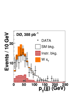
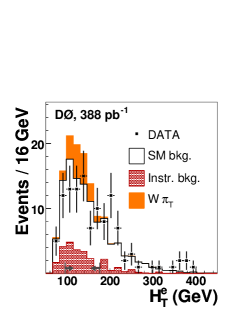
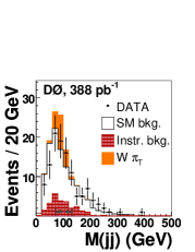
Figure 2: Distributions of and after final kinematic selection. The signal is shown for GeV and GeV. Arrows at
the bottom indicate the cuts applied in the cut-based analysis for the signal mass point shown.
At this point our data sample is still dominated by background. We
therefore use additional variables that characterize the topology of the
events to discriminate between signal and background. These variables are the
azimuthal angle difference between the two jets , the azimuthal
angle difference between the electron and the , ,
the transverse momentum of the dijet system , the scalar sum of the
transverse momenta of the electron and the two jets , the invariant
mass of the dijet system , and the invariant mass of the
boson-dijet system . The technicolor particles are expected to have
narrow widths ( GeV). We should therefore see enhancements in the
distributions of and , consistent in width with the detector
resolution. corresponds to the reconstructed mass and
corresponds to the reconstructed mass. We reconstruct the
boson from the electron and the missing transverse momentum using the boson
mass constraint to solve for of the neutrino. If there are two real
solutions, we take the smaller value of neutrino . If there is only a
complex solution, we take the real part. Distributions of these variables are
shown in Figs. 1 and 2. We use two approaches to
separate signal and background, a cut-based analysis and a neural network
analysis.
The cut-based analysis is optimized using Monte Carlo simulations to
maximize the ratio for every set of technimeson mass values.
is the expected number of events and is the expected number of
background events. For each topological variable, the ratio is evaluated as a function
of the value of the variable to determine a set of lower, upper, or
window cuts which maximizes this ratio.
The neural network analysis uses the topological variables
, , , , the transverse momenta of both jets and
of the electron and . A two-stage neural network based on the Multi Layer Perceptron algorithm NN
is used. The first stage consists of three independent networks which are trained to reject the three main backgrounds, top quark production, production, and all other +jets production including heavy flavors. Each of these three networks has eight input nodes and one hidden layer with 24 nodes. The second stage network has three input nodes, connected to the outputs of the three networks in the first stage, and one hidden layer with six nodes.
The second stage network is trained using all nine physics background processes. The networks are trained separately for each set of technicolor mass values. We then apply the trained neural networks to the collider data, technicolor signals, and
physics and instrumental backgrounds to obtain the discriminator output spectra. We optimize the discriminator cut for every set of techniparticle masses to maximize .
There is no excess in our data over the expected background. We compute upper
limits on the production cross section times branching fraction. In the cut-based
analysis, which is a simple counting experiment, we compute an upper 95% C.L. limit
on the signal using Bayesian statistics d0limit . The neural network analysis
performs a maximum likelihood fit of the data in the
plane to signal and background expectations. The backgrounds are constrained
to their expected values within statistical and systematic
uncertainties.
The uncertainties in the background event yields total to 10–12% and the
uncertainty in the signal selection efficiency is 10% for the cut-based
analysis and 20% for the neural-net based analysis.
The largest contributions to the systematic uncertainties are due to
jet reconstruction efficiency, jet energy scale, -tagging efficiency,
and, only for the signal, from the difference between fast and fully
simulated detector Monte Carlo. The 95% C.L. upper
limit on the signal cross section is then determined by the number of signal
events below which lies 95% of the integral over the resulting likelihood
function.
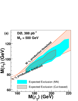
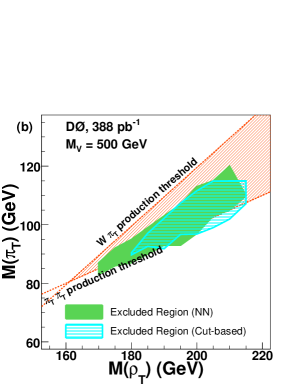
Figure 3: Expected region of exclusion (a) and excluded region (b) at the
95% C.L. in the plane for production with GeV. Kinematic thresholds from and are shown on the figures.
The expected sensitivity and the regions excluded at 95% C.L.
by both analyses in
the plane for GeV are shown in
Fig. 3.
For GeV, only a small region around
GeV and GeV can be excluded.
We note from Fig. 3(a), that the expected sensitivity of
the neural network analysis is
better than that of the cut-based analysis, as indicated by the
larger 95% C.L. exclusion region.
We quote the observed 95% C.L. exclusion region
in the plane in Fig. 3(b) by the neural
network analysis as our measurement footnote .
The results presented in this paper cannot be compared directly to
those previously published PreviousTC . The CDF
experiment did not use Ref. Lane2 and Lane4 ,
but rather the models described in the earlier paper of
Ref. Lane1 , a precursor to the TCSM. The LEP
experiments used Ref. Lane2 in which the
cross sections, while appropriate for narrow production in collisions, are incorrect for off-resonance production in
collisions such as at LEP (see Ref. Lane3 ).
Although differences in the employed TC models preclude a direct comparison with previous searches, the current search
achieves a higher sensitivity to the considered physics process.
We thank Ken Lane for helpful discussions,
the staffs at Fermilab and collaborating institutions,
and acknowledge support from the
DOE and NSF (USA);
CEA and CNRS/IN2P3 (France);
FASI, Rosatom and RFBR (Russia);
CAPES, CNPq, FAPERJ, FAPESP and FUNDUNESP (Brazil);
DAE and DST (India);
Colciencias (Colombia);
CONACyT (Mexico);
KRF and KOSEF (Korea);
CONICET and UBACyT (Argentina);
FOM (The Netherlands);
PPARC (United Kingdom);
MSMT (Czech Republic);
CRC Program, CFI, NSERC and WestGrid Project (Canada);
BMBF and DFG (Germany);
SFI (Ireland);
The Swedish Research Council (Sweden);
Research Corporation;
Alexander von Humboldt Foundation;
and the Marie Curie Program.
References
(1)
On leave from IEP SAS Kosice, Slovakia.
(2)
Visitor from Helsinki Institute of Physics, Helsinki, Finland.
(3)
S. Weinberg, Phys. Rev. D 13, 974 (1976).
(4)
L. Susskind, Phys. Rev. D 20, 2619 (1979).
(5)
S. Dimopoulos and L. Susskind, Nucl. Phys. B155, 237 (1979).
(6)
E. Eichten and K. Lane, Phys. Lett. 90B, 125 (1980).
(7)
B. Holdom, Phys. Rev. D 24, 1441 (1981).
Phys. Lett. 150B, 301 (1985).
T. Appelquist, D. Karabali, and L. C. R. Wijewardhana,
Phys. Rev. Lett. 57, 957 (1986).
(8)
C. T. Hill, Phys. Lett. B 345, 483 (1995).
(9)
K. Lane and E. Eichten, Phys. Lett. B 222, 274 (1989).
(10)
K. Lane, Phys. Rev. D60, 075007 (1999).
(11)
K. Lane and S. Mrenna, Phys. Rev. D67, 115011 (2003).
(12)
DØ Collaboration, V.M. Abazov, et al., Nucl. Instrum. and Methods A 565, 463 (2006).
(13)
G. Blazey et al., in Proceedings of the Workshop: “QCD and Weak Boson Physics in Run II,” edited by U. Baur, R.K. Ellis and D. Zeppenfeld (Fermilab, Batavia, IL, 2000), p.47; see Sec. 3.5 for details.
(14)
T. Edwards et al., FERMILAB-TM-2278-E (2004).
(15)
T. Sjöstrand et al., Comput. Phys. Commun. 135, 238 (2001). We use pythia version 6.224.
(16)
F. Caravaglios, M. L. Mangano, M. Moretti and R. Pittau, Nucl. Phys. B 539 215 (1999).
(17)
R. Brun and F. Carminati, CERN Program Library Long Writeup W5013, 1993 (unpublished).
(18)
and is the polar angle with respect
to the proton beam direction.
(19)
H. L. Lai, et al., Eur. Phys. J. C 12, 375 (2000).
(20)
R. Hamberg, W. L. Van Neerven, and T. Matsura, Nucl. Phys. B359, 343 (1991).
(23)
Consistent scaling of luminosity and background prior to optimization,
using the new D0 luminosity newlumi
will lead to somewhat better limits. Nevertheless,
we choose to keep the analysis consistent with the previous estimate
of the luminosity value oldlumi .
(24)
T. Andeen et. al., FERMILAB-TM-2365-E (2006), in preparation.
(25)
CDF Collaboration, T. Affolder et al., Phys. Rev. Lett. 84,
1110 (2000);
DELPHI Collaboration, J. Abdallah et al., Eur. Phys. J. C 22,
17 (2001).
(26) K. Lane, Lectures at Frascati Spring School,
Technicolor 2000, Frascati, Rome, Italy, 2000; hep-ph/0007304.