Measurement of ${\cal{B}}(\Upsilon(5S)\to B_{s}^{(*)}\overline{B_{s}}^{(*)})$ Using $\phi$ Mesons

Abstract

Knowledge of the $B_{s}$ decay fraction of the $\Upsilon$(5S) resonance, $f_{S}$, is important for $B_{s}$ meson studies at the $\Upsilon(5S)$ energy. Using a data sample collected by the CLEO III detector at CESR consisting of 0.423 fb^-1 on the $\Upsilon$(5S) resonance, 6.34 fb^-1 on the $\Upsilon$(4S) and 2.32 fb^-1 in the continuum below the $\Upsilon$(4S), we measure ${\cal{B}}(\Upsilon(5S)\to\phi X)=(13.8\pm 0.7^{+2.3}_{-1.5})\%$ and ${\cal{B}}(\Upsilon(4S)\to\phi X)=(7.1\pm 0.1\pm 0.6)\%$; the ratio of the two rates is $(1.9\pm 0.1^{+0.3}_{-0.2})$. This is the first measurement of the $\phi$ meson yield from the $\Upsilon$(5S). Using these rates, and a model dependent estimate of ${\cal{B}}(B_{s}\to\phi X)$, we determine $f_{S}=(24.6\pm 2.9^{+11.0}_{-~{}5.3})\%$. We also update our previous independent measurement of $f_{S}$ made using the inclusive $D_{s}$ yields to now be $(16.8\pm 2.6^{+6.7}_{-3.4})\%$, due to a better estimate of the number of hadronic events. We also report the total $\Upsilon(5S)$ hadronic cross section above continuum to be $\sigma(e^{+}e^{-}\to\Upsilon(5S))=(0.301\pm 0.002\pm 0.039)$ nb. This allows us to extract the fraction of $B$ mesons as $(58.9\pm 10.0\pm 9.2)$%, equal to 1-$f_{S}$. Averaging the three methods gives a model dependent result of $f_{S}=(21^{+6}_{-3})$%.

I Introduction

The putative $\Upsilon$(5S) resonance was discovered at CESR long ago by the CLEO 5s_cleo and CUSB 5s_cusb collaborations by observing an enhancement in the total $e^{+}e^{-}$ annihilation cross-section into hadrons at a center-of-mass energy of about 40 MeV above the $B_{s}^{*}\overline{B_{s}}^{*}$ production threshold. Its mass and its production cross-section were measured as (10.865$\pm$0.008) GeV/$c^{2}$ and about 0.35 nb, respectively 5s_cleo .

The possible final states of the $\Upsilon$(5S) resonance decays are: $B_{s}^{*}\overline{B_{s}}^{*}$, $B_{s}\overline{B_{s}}^{*}$, $B_{s}\overline{B_{s}}$, $B^{*}\overline{B}^{*}$, $B\overline{B}^{*}$, $B\overline{B}$, $B\overline{B}\pi$, $B\overline{B}^{*}\pi$, $B^{*}\overline{B}^{*}\pi$, $B\overline{B}\pi\pi$, where the $B$ and $\pi$ mesons can be either neutral or charged. Several models involving coupled channel calculations have predicted the cross-section and final state composition Models ; UQM . The Unitarized Quark Model UQM , for example, predicts that the total $b\overline{b}$ cross-section at the $\Upsilon$(5S) energy is dominated by $B^{*}\overline{B}^{*}$ and $B_{s}^{*}\overline{B}_{s}^{*}$ production, with $B_{s}$ production accounting for about 1/3 of the total rate. The original $\sim$116 pb^-1 of data collected at CESR did not reveal if any $B_{s}$ mesons were produced. By measuring the inclusive $D_{s}$ production rate using CLEO III data we previously measured the fraction of $B_{s}$ meson production at the $\Upsilon$(5S), $f_{S}$, to be $(16.0\pm 2.6\pm 5.8)\%$ of the total $b\overline{b}$ rate Incl_Bs_5s ; this measurement uses a theoretical estimate of ${\cal{B}}(B_{s}\to D_{s}X)=(92\pm 11)\%$ Incl_Bs_5s .

$B_{s}$ production was confirmed in a second CLEO analysis Excl_Bs_5s that fully reconstructed $B_{s}$ meson decays. In addition, this analysis showed that the final states are dominated by the $B_{s}^{*}\overline{B}_{s}^{*}$ decay channel. These results have been confirmed by the Belle collaboration Belle . A third CLEO analysis of the exclusive $B$ reconstruction at the $\Upsilon$(5S) showed that the $B\overline{B}X$ final states in $\Upsilon$(5S) decays are dominated by $B^{*}\overline{B}^{*}$ with a considerable contribution from $B\overline{B}^{*}$ and $B^{*}\overline{B}$ final states B_5s .

Knowledge of the $B_{s}$ production rate at the $\Upsilon$(5S) resonance, $f_{S}$, is necessary to compare with predictions of theoretical models of $b$-hadron production. More importantly, $f_{S}$ is also essential for evaluating the possibility of $B_{s}$ studies at the $\Upsilon$(5S) using current $B$-factories, and for future $e^{+}e^{-}$ Super-$B$ Factories, should they come to fruition, where precision measurements of $B_{s}$ decays are an important goal superb . However, the determination of $f_{S}$ in a model independent manner requires several tens of fb^-1 5s_Theory . In this paper, we improve our knowledge of the $B_{s}$ production at the $\Upsilon$(5S) by using inclusive $\phi$ meson yields to make a second model dependent measurement of ${\cal{B}}(\Upsilon(5S)\to B_{s}^{*}\overline{B_{s}}^{*})$.

We choose to examine $\phi$ meson yields because they will be produced much more often in $B_{s}$ decays than in $B$ decays. The branching fractions of $B_{s}$ to $D_{s}$ mesons and $B$ to $D$ mesons are of order 1, while the rates of $B_{s}$ to $D$ mesons and $B$ to $D_{s}$ mesons are on the order of 1/10. We also know that the production rate of $\phi$ mesons is one order of magnitude higher in $D_{s}$ decays than in $D^{0}$ and $D^{+}$ decays as measured using recent CLEO-c data D_Ds_incl . These results are shown in Table 1. The rate of $D$ mesons into $\phi$ mesons is only 1%, while the rate of $D_{s}$ mesons into $\phi$ mesons is 16%.

Table 1: $D^{0}$, $D^{+}$ and $D_{s}^{+}$ inclusive branching ratios into $\phi$ mesons. The $D$ meson decays used 281 pb^-1 of data at the $\psi(3770)$, while the $D_{s}$ decays were measured using 195 pb^-1 at or near 4170 MeV.

	${\cal{B}}(D\to\phi X$)(%)
$D^{0}$	$1.05\pm 0.08\pm 0.07$
$D^{+}$	$1.03\pm 0.10\pm 0.07$
$D_{s}^{+}$	$16.1\pm 1.2\pm 1.1$

Since the $B\to\phi X$ branching ratio already has been measured to be $(3.42\pm 0.13)\%$ PDG , we expect a large difference between the $\phi$ yields at the $\Upsilon$(5S) and at the $\Upsilon$(4S), due to the presence of $B_{s}$, that we will use to measure the size of the $B_{s}^{(*)}\overline{B_{s}}^{(*)}$ component at the $\Upsilon$(5S). The analysis technique used here is similar to the one used in Incl_Bs_5s . We also present an update to the first measurement of $f_{S}$ that used $D_{s}$ yields Incl_Bs_5s , and we report on the measurement of the total $\Upsilon$(5S) hadronic cross-section. When we discuss the $\Upsilon$(5S) here, we mean any production above what is expected from continuum production of quarks lighter than the $b$ at an $e^{+}e^{-}$ center-of-mass energy of 10.865 GeV.

The CLEO III detector is equipped to measure the momenta and directions of charged particles, identify charged hadrons, detect photons, and determine with good precision their directions and energies. It has been described in detail previously CLEO_DR ; CLEO_RICH .

II Measurement of ${\cal{B}}(\Upsilon(5S)\to B_{s}^{(*)}\overline{B_{s}}^{(*)})$ Using $\phi$ Meson Yields

II.1 Data Sample and Signal Selection

We use 6.34 fb^-1 integrated luminosity of data collected on the $\Upsilon(4S$) resonance peak and 0.423 fb^-1 of data collected on the $\Upsilon(5S)$ resonance ($E_{CM}=10.868~{}\rm GeV$). A third data sample of 2.32 fb^-1 collected in the continuum 40 MeV in center-of-mass energy below the $\Upsilon(4S)$ is used to subtract the four-flavor ($u$, $d$, $s$ and $c$ quark) continuum events.

Hadronic events are selected using criteria based on the number of charged tracks and the amount of energy deposited in the electromagnetic calorimeter. To select “spherical” $b$-quark events we require that the Fox-Wolfram shape parameter Fox , $R_{2}$, be less than $0.25$. $\phi$ meson candidates are looked for through the reconstruction of a pair of oppositely charged tracks identified as kaons. These tracks are required to originate from the main interaction point and have a minimum of half of the maximal number of hits in the tracking chambers. They also must satisfy kaon identification criteria that uses information from both the Ring Imaging Cherenkov (RICH) and the ionization loss in the drift chamber, $dE/dx$, of the CLEO III detector. Kaon identification has been described in detail previously Incl_Bs_5s .

II.2 $\phi$ Meson Yields From $\Upsilon$(5S) and $\Upsilon$(4S) Decays

All pairs of oppositely charged kaon candidates were examined for $\phi$ candidates if their summed momenta is less than half of the beam energy. Instead of momentum we choose to work with the variable $x$ which is the $\phi$ momentum divided by the beam energy, to remove differences caused by the the change of energies between continuum data taken just below the $\Upsilon$(4S), at the $\Upsilon$(4S) and at the $\Upsilon$(5S). The $K^{+}K^{-}$ invariant mass distributions for $x\leq 0.5$ are shown in Fig. 1.

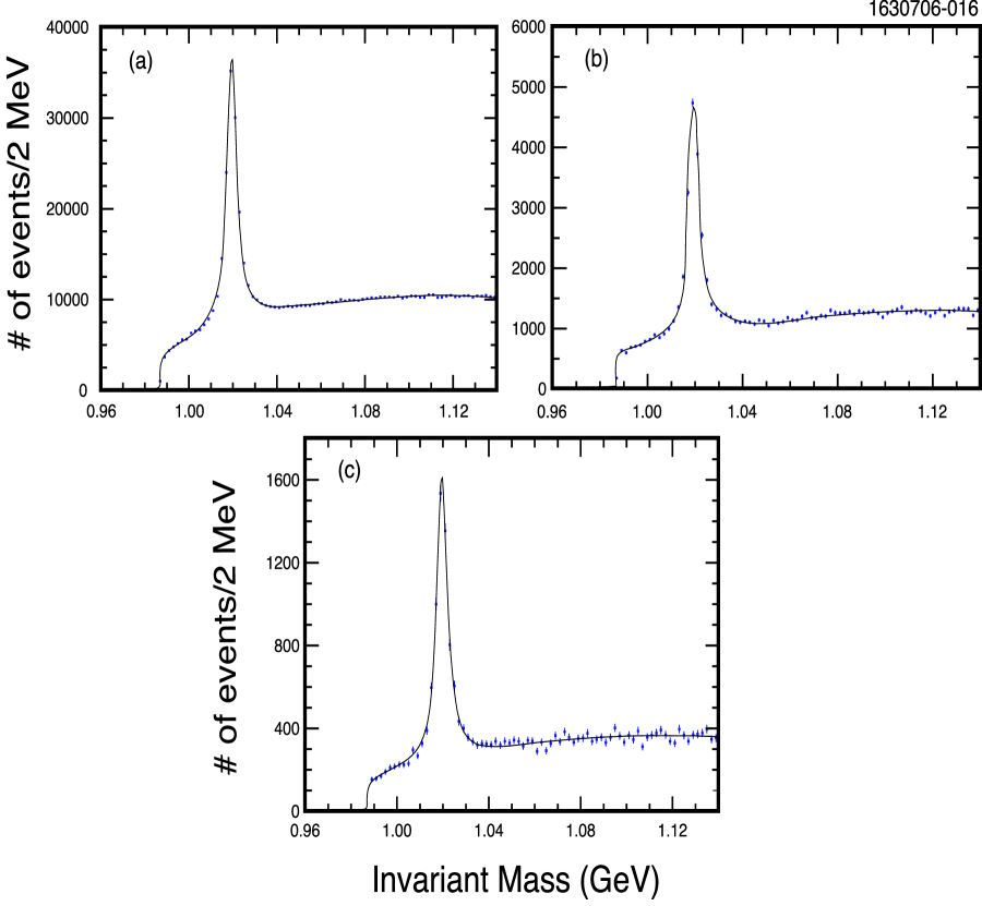
Figure 1: The invariant mass distributions of the $\phi$ candidates with $x\leq$ 0.5 from: (a) the $\Upsilon$(4S) on-resonance data (b) the continuum below the $\Upsilon$(4S) resonance data, and (c) the $\Upsilon$(5S) on-resonance data. The solid line is the fit to the signal and background shapes explained in the text.

II.2.1 $K^{+}K^{-}$ Invariant Mass Spectra and Yields

A crucial aspect in this analysis is to accurately model the signal and background shapes. For the signal we use a Breit-Wigner signal shape convoluted with a Gaussian. The width of the Breit-Wigner function was fixed to the natural width of the $\phi$ meson, $\Gamma_{1}=4.26~{}\rm MeV$ PDG . It is convoluted here with a Gaussian function to allow the integration of the detector resolution into the signal function. A second Gaussian is added for an adequate fitting of the tails. The form of the signal fitting function, where the dependent variable $\zeta$ is the invariant mass of our $K^{+}K^{-}$ candidates, is given by

$$S(\zeta)=h(\zeta)+\int_{\zeta-5\sigma}^{\zeta+5\sigma}{f(y)g(\zeta-y)dy}.$$ (1)

Here, at every physical point $\zeta$, the Breit-Wigner function

$$f(y)=\frac{1}{2\pi}\cdot\frac{A_{1}\cdot{\Gamma_{1}}}{[(y-\overline{y})^{2}+\frac{\Gamma_{1}^{2}}{4}]}~{}$$ (2)

is convoluted with the Gaussian

$$g(\zeta-y)=\frac{1}{\sqrt{2\pi}\sigma_{2}}~{}\exp\left[\frac{(\zeta-y)^{2}}{2\sigma_{2}^{2}}\right]~{}.$$ (3)

The integration over $y$ is between the limits $\zeta-5\sigma$, and $\zeta+5\sigma$. $A_{1}$ and $\overline{y}$ are the area and mean value of the Breit-Wigner, and $\sigma_{2}$ is the standard deviation of the Gaussian. $h(\zeta)$ is a second Gaussian added to fit the tails.

The background shape is given by a function, chosen to model the threshold, that has the following functional form:

$$B(\zeta)=A\cdot{{(\zeta-\zeta_{0})}^{p}}\cdot{\exp~{}{[c_{1}(\zeta-\zeta_{0})+c_{2}(\zeta-\zeta_{0})^{2}]}},$$ (4)

where $A$ is the normalization, $\zeta_{0}$ is the threshold, $p$ is the power of a polynomial about the turn-on point, and $c_{1}$ and $c_{2}$ are linear and quadratic coefficients in the exponential. Because this function has a sharp rise followed by an exponential tail, we are able to accurately describe the threshold behavior at low invariant mass close to the kinematic limit.

We show the invariant mass of the $K^{+}K^{-}$ candidates in 9 different $x$ intervals (from 0.05 to 0.50) for all the data samples in Fig. 2, Fig. 3 and Fig. 4.

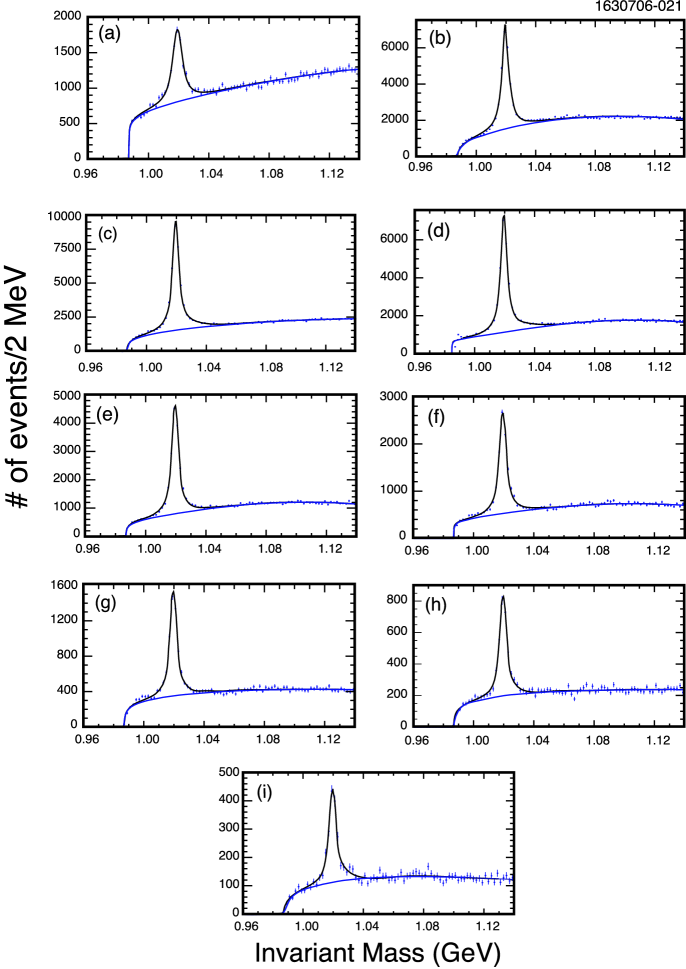
Figure 2: The $K^{+}K^{-}$ mass combinations from $\Upsilon$(4S) on-resonance data, fitted to the sum of a Breit-Wigner signal shape centered at the nominal $\phi$ mass, convoluted with a Gaussian to describe the detector resolution, and a second Gaussian distribution for a better parametrization of the tails. The background is parameterized by a threshold function (see text). These distributions are in the $x$ intervals: (a) $0.05<x<0.10$, (b) $0.10<x<0.15$, (c) $0.15<x<0.20$, (d) $0.20<x<0.25$, (e) $0.25<x<0.30$, (f) $0.30<x<0.35$, (g) $0.35<x<0.40$, (h) $0.40<x<0.45$, (i) $0.45<x<0.50$.

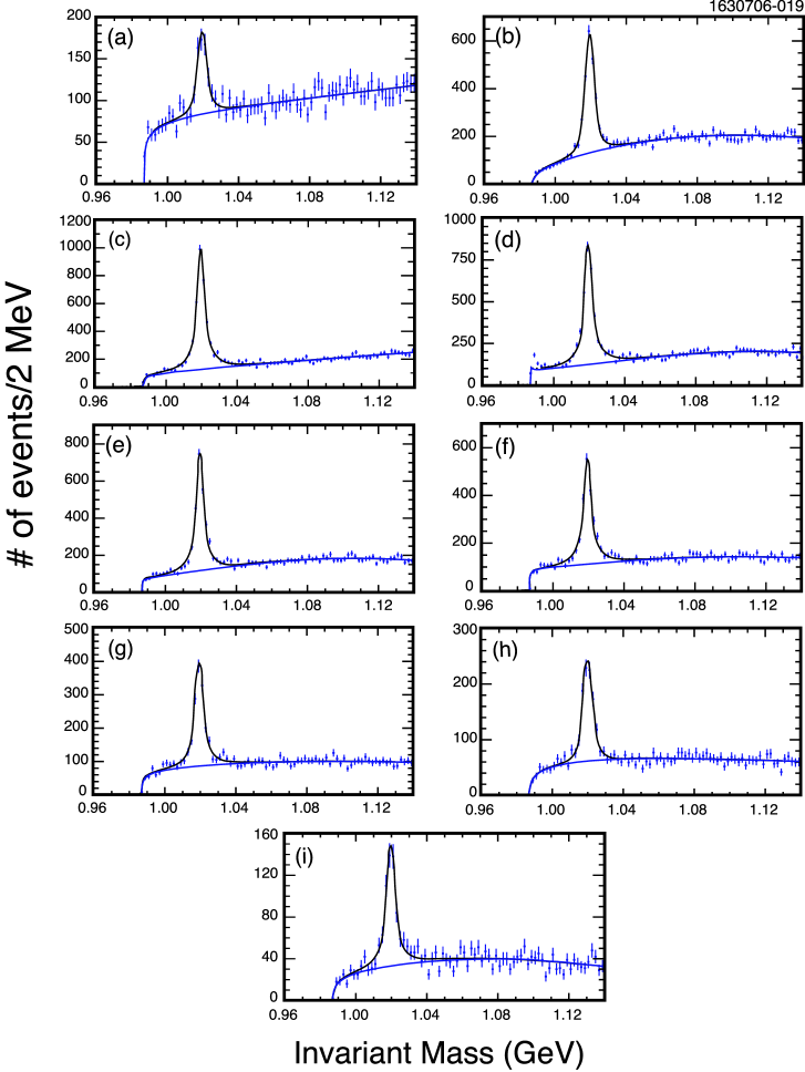
Figure 3: The $K^{+}K^{-}$ mass combinations from the continuum below the $\Upsilon$(4S), fitted to the sum of a Breit-Wigner signal shape centered at the nominal $\phi$ mass, convoluted with a Gaussian to describe the detector resolution, and a second Gaussian distribution for a better parametrization of the tails. The background is parameterized by a threshold function (see text). These distributions are in the $x$ intervals: (a) $0.05<x<0.10$, (b) $0.10<x<0.15$, (c) $0.15<x<0.20$, (d) $0.20<x<0.25$, (e) $0.25<x<0.30$, (f) $0.30<x<0.35$, (g) $0.35<x<0.40$, (h) $0.40<x<0.45$, (i) $0.45<x<0.50$.

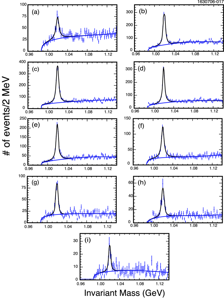
Figure 4: The $K^{+}K^{-}$ mass combinations from the $\Upsilon$(5S), fitted to the sum of a Breit-Wigner signal shape centered at the nominal $\phi$ mass, convoluted with a Gaussian to describe the detector resolution, and a second Gaussian distribution for a better parametrization of the tails. The background is parameterized by a threshold function (see text). These distributions are in the $x$ intervals: (a) $0.05<x<0.10$, (b) $0.10<x<0.15$, (c) $0.15<x<0.20$, (d) $0.20<x<0.25$, (e) $0.25<x<0.30$, (f) $0.30<x<0.35$, (g) $0.35<x<0.40$, (h) $0.40<x<0.45$, (i) $0.45<x<0.50$.

We determine the raw yield of $\phi$’s shown in Fig. 5 (a), (b) and (c) from fits of the invariant mass distributions to the functions $S(\zeta)$ and $B(\zeta)$ defined above. All the parameters in $S(\zeta)$ in all the fits, except the yields, were fixed to the values obtained when fitting the corresponding distributions from the sum of the three data samples collected at the three different beam energies in each $x$ interval separately. The parameters describing $B(\zeta)$, on the other hand, are allowed to float except for $\zeta_{0}$ which is fixed to twice the $K^{+}$ mass. The yields are listed in the second and third columns of Table 2 and Table 3.

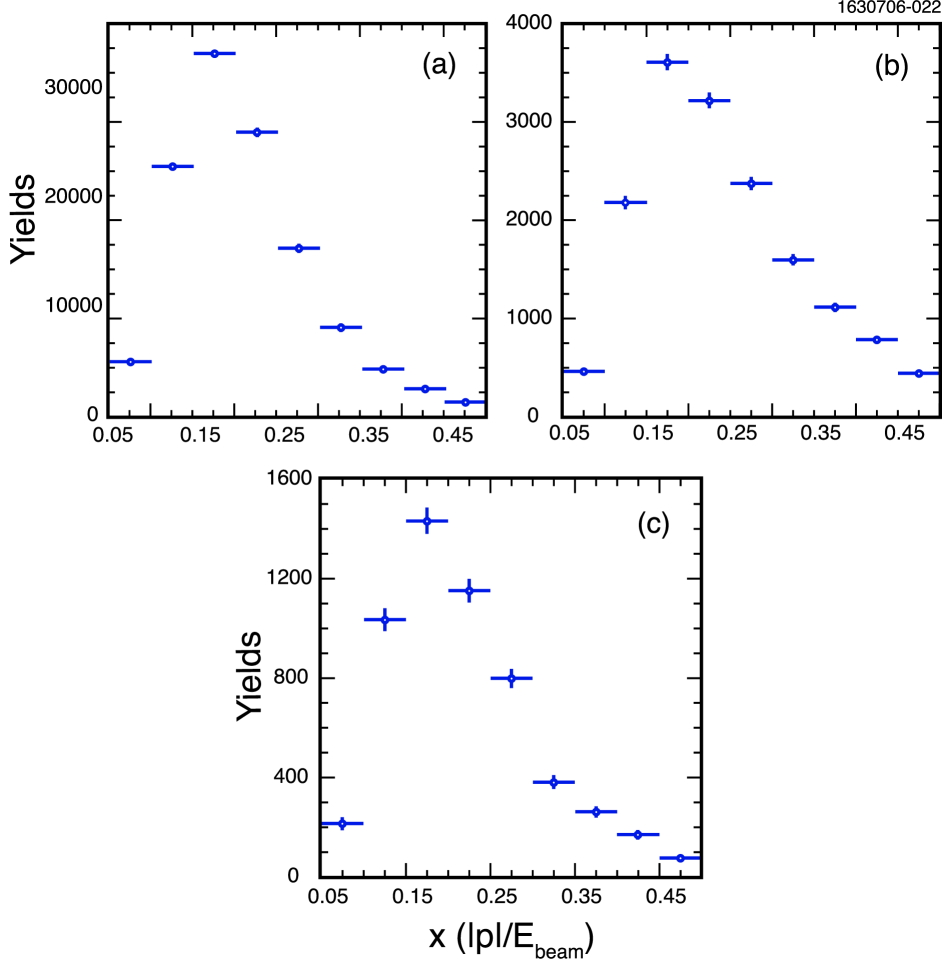
Figure 5: Raw $\phi$ yields from: (a) the $\Upsilon$(4S) data, (b) the continuum below the $\Upsilon$(4S) data, (c) the $\Upsilon$(5S) data.

The systematic errors on these yields are estimated to be $\pm 4\%$, and are obtained by varying the fitting techniques. One variation is to float the fitting parameters at the different beam energies, instead of fixing them. We also used different functions including a Breit-Wigner signal shape with and without convolution, or a double Guassian shape for the signal, and for background either other threshold functions or polynomials.

Table 2: $\phi$ yields from the $\Upsilon$(4S) ($N^{i}_{\Upsilon(4S)on}$), from the continuum below the $\Upsilon$(4S) ($N^{i}_{cont}$), and from the continuum subtracted $\Upsilon$(4S) ($N^{i}_{\Upsilon(4S)}$). Also listed are the $\phi$ reconstruction efficiencies ($\epsilon^{i}$), and the partial $\Upsilon(4S)\to\phi X$ branching fractions as a function of $x$. The systematic errors on the yields are $\pm 4\%$.

$x^{i}$($\frac{|p^{i}|}{E_{beam}}$)	$N^{i}_{\Upsilon(4S)on}$	$N^{i}_{cont}$	$N^{i}_{\Upsilon(4S)}$	$\epsilon^{i}(\%)$	$B^{i}$(%)
0.05-0.10	$4938.1\pm 135.2$	$462.4\pm 41.0$	$3683.5\pm 175.1$	$8.0$	$1.46\pm 0.09$
0.10-0.15	$22848.9\pm 228.7$	$2179.0\pm 69.0$	$16937.3\pm 295.5$	$31.9$	$1.68\pm 0.04$
0.15-0.20	$33207.4\pm 269.1$	$3608.7\pm 84.1$	$23417.2\pm 352.8$	$47.1$	$1.57\pm 0.03$
0.20-0.25	$26020.4\pm 237.6$	$3218.7\pm 80.7$	$17288.3\pm 323.1$	$51.3$	$1.06\pm 0.03$
0.25-0.30	$15364.1\pm 178.8$	$2374.2\pm 69.4$	$8923.0\pm 259.7$	$49.1$	$0.58\pm 0.02$
0.30-0.35	$8107.8\pm 128.2$	$1597.6\pm 57.8$	$3773.5\pm 202.5$	$42.3$	$0.28\pm 0.02$
0.35-0.40	$4263.5\pm 95.9$	$1113.4\pm 48.6$	$1242.9\pm 162.9$	$35.8$	$0.11\pm 0.01$
0.40-0.45	$2475.3\pm 75.1$	$786.6\pm 42.3$	$341.2\pm 137.1$	$21.6$	$0.05\pm 0.02$
0.45-0.50	$1256.9\pm 57.6$	$443.6\pm 30.9$	$53.5\pm 101.8$	$13.4$	$0.01\pm 0.02$

Table 3: $\phi$ yields from the $\Upsilon$(5S) ($N^{i}_{\Upsilon(5S)on}$), from the continuum below the $\Upsilon$(4S) ($N^{i}_{cont}$ are the same as in the previous table), and from the continuum subtracted $\Upsilon$(5S) continuum subtracted ($N^{i}_{\Upsilon(5S)}$). Also listed are the $\phi$ reconstruction efficiencies ($\epsilon^{i}$ which are taken to be the same as in the previous table), and the partial $\Upsilon(5S)\to\phi X$ branching fractions as a function of $x$. The systematic errors on the yields are $\pm 4\%$.

$x^{i}$($\frac{|p^{i}|}{E_{beam}}$)	$N^{i}_{\Upsilon(5S)on}$	$N^{i}_{cont}$	$N^{i}_{\Upsilon(5S)}$	$\epsilon^{i}(\%)$	$B^{i}$(%)
0.05-0.10	$214.7\pm 26.2$	$462.4\pm 41.0$	$135.3\pm 27.1$	$8.0$	$2.7\pm 0.6$
0.10-0.15	$1034.8\pm 46.0$	$2179.0\pm 69.0$	$660.4\pm 47.5$	$31.9$	$3.3\pm 0.2$
0.15-0.20	$1432.5\pm 53.0$	$3608.7\pm 84.1$	$812.4\pm 54.9$	$47.1$	$2.8\pm 0.2$
0.20-0.25	$1151.9\pm 47.3$	$3218.7\pm 80.7$	$598.9\pm 49.3$	$51.3$	$1.9\pm 0.2$
0.25-0.30	$789.2\pm 38.6$	$2374.2\pm 69.4$	$390.2\pm 40.4$	$49.1$	$1.3\pm 0.1$
0.30-0.35	$382.3\pm 27.9$	$1597.6\pm 57.8$	$107.8\pm 29.7$	$42.3$	$0.4\pm 0.1$
0.35-0.40	$261.2\pm 22.7$	$1113.4\pm 48.6$	$70.0\pm 24.1$	$35.8$	$0.3\pm 0.1$
0.40-0.45	$169.7\pm 19.1$	$786.6\pm 42.3$	$34.5\pm 20.4$	$21.6$	$0.3\pm 0.2$
0.45-0.50	$75.0\pm 13.6$	$443.6\pm 30.9$	$-1.2\pm 14.6$	$13.4$	$-0.1\pm 0.2$

II.2.2 Continuum Subtraction

The numbers of hadronic events and $\phi$ candidates from the $\Upsilon$(5S) and the $\Upsilon$(4S) resonance decays are determined by subtracting the scaled four-flavor ($u$, $d$, $s$ and $c$ quarks) continuum events from the $\Upsilon$(4S) and the $\Upsilon$(5S) data. The scale factors, $S_{nS}$, are determined using the same technique described in Incl_Bs_5s , where

$$S_{nS}={\frac{L_{nS}}{L_{\rm cont}}}\cdot{\left({\frac{E_{\rm cont}}{E_{nS}}}\right)^{2}}~{}$$ (5)

with $L_{nS}$, $L_{\rm cont}$, $E_{nS}$ and $E_{\rm cont}$ being the collected luminosities and the center-of-mass energies at the $\Upsilon$(nS) and at the continuum below the $\Upsilon$(4S). We find:

$$S_{4S}={2.713\pm 0.001\pm 0.027}~{},$$ (6)

and

$$S_{5S}={(17.18\pm 0.01\pm 0.17)}\cdot{10^{-2}}~{}.$$ (7)

We estimate the systematic error on these scale factors by obtaining them in a different manner. Here we measure the ratio of the number of charged tracks at the different beam energies in the $0.6<x<0.8$ interval. The lower limit on the $x$ interval used here is determined by the maximum value tracks from $B\overline{B}$ events can have, including smearing because of the measuring resolution, and the upper limit is chosen to eliminate radiative electromagnetic processes. Since the tracks should be produced only from continuum events, we suppress beam-gas and beam-wall interactions, photon pair and $\tau$ pair events using strict cuts on track multiplicities, event energies and event shapes. Since particle production may be larger at the higher $\Upsilon(5S)$ energy than the continuum below the $\Upsilon(4S)$, we apply a small multiplicative correction of (1.016$\pm$0.011)%, as determined by Monte Carlo simulation to the relative track yields. Track counting gives a 1% lower value for $S_{5S}$ and we use this difference as our estimate of the systematic error. Note, that the error on the beam energy (0.1%) has a negligible effect.

These numbers are updated from those reported in Incl_Bs_5s , due to an increase in Monte Carlo statistics, and the use of a more precise calibration of the beam energy.

II.2.3 $\phi$ Reconstruction Efficiency

The $x$ dependent $\phi$ detection efficiency shown in Fig. 6 is determined by reconstructing and fitting $\phi$ candidates in more than 8 million simulated $B\overline{B}$ generic decays.

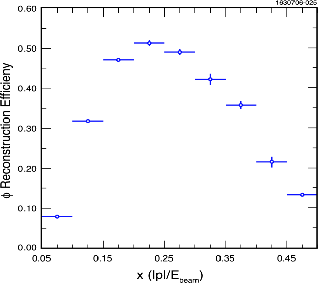
Figure 6: $\phi$ reconstruction efficiency from more than 8 million $B\overline{B}$ Monte Carlo simulated events. The errors are statistical only.

The low reconstruction efficiency at small $x$ is due to the fact that as the $\phi$ becomes less energetic, it becomes more probable that it is formed of a slow kaon (with momentum below $0.2~{}\rm GeV/c$) whose detection is very inefficient, since it is likely to be absorbed in the beam-pipe or vertex detector material. The efficiency for large $x$ ($0.4<x<0.5$) is somewhat lower than naively expected because of the $R_{2}$ cut of 0.25. Due to the low efficiency and large backgrounds in the first bin, $x<0.05$, we do not measure the $\phi$ yield in this interval, but will rely on a model of $\phi$ production to extract a value.

II.2.4 $\phi$ Branching Ratios

To find the number of hadronic decays produced above the four-flavor continuum, denoted as $N^{Res}_{\Upsilon(nS)}$, we multiply the number of events found in the continuum below the $\Upsilon$(4S), $N^{off}_{\Upsilon(4S)}$, by the $S_{4S}$ and $S_{5S}$ scale factors, and subtract them from the number of hadronic events found at each resonance, $N^{on}_{\Upsilon(nS)}$:

$$N^{\rm Res}_{\Upsilon(4S)}=N^{\rm on}_{\Upsilon(4S)}-S_{4S}\cdot N^{\rm off}_{\Upsilon(4S)}=(6.42\pm 0.01\pm 0.26)\cdot{10^{6}}~{}$$ (8)

$$N^{\rm Res}_{\Upsilon(5S)}=N^{\rm on}_{\Upsilon(5S)}-S_{5S}\cdot N^{\rm off}_{\Upsilon(5S)}=(0.127\pm 0.001\pm 0.016)\cdot{10^{6}}~{}.$$ (9)

Using these numbers together with $N^{i}_{\Upsilon(4S)}$ ($N^{i}_{\Upsilon(5S)}$) and $\epsilon^{i}$ which are the $\phi$ yield and $\phi$ reconstruction efficiency in the $i$-th $x$ interval respectively, we measure the inclusive partial decay rate of the $\Upsilon$(nS) resonance into $\phi$ mesons in the $i$-th $x$ interval as follows:

$${\cal{B}}^{i}(\Upsilon(nS)\to\phi X)={\frac{1}{N^{Res}_{\Upsilon(nS)}\times{{\cal{B}}(\phi\to K^{+}K^{-})}}}~{}\left({\frac{N^{i}_{\Upsilon(nS)}}{\epsilon^{i}}}\right)~{}\\$$ (10)

The results are listed in the last column of Table 2 and Table 3 and shown in Fig. 7.

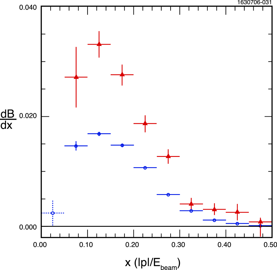
Figure 7: The efficiency corrected $\phi$ branching ratio in each $x$ interval from the $\Upsilon$(5S) resonance decays (triangles), and from the $\Upsilon$(4S) resonance decays (open circles). Errors are statistical only, except for the first bin where the $\Upsilon$(4S) data point is a theoretical estimate based on Monte Carlo, with an error equal to its value.

Summing the results for $0.05<x<0.50$ we measure

$${\cal{B}}^{(x>0.05)}(\Upsilon(4S)\to\phi X)=(6.82\pm 0.09\pm 0.55)\%.~{}$$ (11)

As the rate in the first interval 0.00$<x<$0.05 is experimentally not accessible in this analysis, we estimate the branching fraction in this interval using our Monte Carlo simulation to model $\phi$ production. This interval has 3.6% of the total $\phi$ yield, which corresponds to a branching fraction of 0.24%. We take the error as equal to the value. The total production rate then is

$${\cal{B}}(\Upsilon(4S)\to\phi X)=(7.06\pm 0.09\pm 0.60)\%,~{}$$ (12)

that when divided by two gives the $B$ meson branching fraction into $\phi$ mesons of

$${\cal{B}}(B\to\phi X)=(3.53\pm 0.05\pm 0.30)\%~{},$$ (13)

which is in good agreement with the PDG PDG value of $(3.42\pm 0.13)\%$. For the $\Upsilon$(5S) we measure for $x>0.05$

$${\cal{B}}^{(x>0.05)}(\Upsilon(5S)\to\phi X)=(12.9\pm 0.7^{+2.2}_{-1.4})\%.~{}$$ (14)

In addition, we find for $x>0.05$

$$\frac{{\cal{B}}(\Upsilon(5S)\to\phi X)}{{\cal{B}}(\Upsilon(4S)\to\phi X)}=1.9\pm 0.1^{+0.3}_{-0.2}~{}.$$ (15)

This result is more than $9.6\sigma$ significant, including both the statistical and the systematic errors, thus demonstrating an almost factor of two larger production of $\phi$ mesons at the $\Upsilon$(5S) than at the $\Upsilon$(4S).

II.2.5 Determination of The Statistical and Systematic Uncertainties

Since the measurements presented in the previous section depend on a large number of parameters, the corresponding errors on those measurements can have highly correlated contributions. In this section, we explain the method we used to extract the statistical and the systematic errors on our measurements by taking into account the sources of correlations between the different parameters.

We measure the $\phi$ production rate at the $\Upsilon$(4S) and $\Upsilon$(5S) using

$${{\cal{B}}^{(x>0.05)}(\Upsilon({\rm nS})\to\phi X)}=\frac{1}{N^{\rm Res}_{\Upsilon(nS)}\cdot{\cal{B}}_{1}}~{}{{\sum_{i=2}^{10}{\frac{N^{i}_{\Upsilon(nS)}}{\epsilon^{i}}}}}$$ (16)

$$~{}~{}~{}~{}~{}~{}~{}~{}~{}~{}~{}~{}~{}~{}~{}~{}=\frac{1}{({N^{\rm h}_{\Upsilon(nS)on}-S_{n}\cdot N^{h}_{\rm cont}})\cdot{\cal{B}}_{1}}~{}{{\sum_{i=2}^{10}{\frac{N^{i}_{\Upsilon(nS)on}-S_{n}\cdot N^{i}_{\rm cont}}{\epsilon^{i}}}}}~{}.~{}$$

The quantities in this equation are defined as:

• $N^{Res}_{\Upsilon(nS)}$ is the number of hadronic events at the $\Upsilon$(nS) energy after continuum subtraction.

• $N^{\rm h}_{\Upsilon(nS)on}$ and $N^{h}_{\rm cont}$ are respectively the number of hadronic events from the data taken at the $\Upsilon$(nS) energy and from the continuum data taken at $30~{}\rm MeV$ below the $\Upsilon$(4S) resonance.

• ${\cal{B}}_{1}$ is the ${\cal{B}}(\phi\to K^{+}K^{-})$ branching fraction of 49.1% PDG .

• $N^{i}_{\Upsilon(nS)}$ is the number of $\phi$ candidates in the $i$-th $x$ interval from the $\Upsilon$(nS) resonance events (i.e. after continuum subtraction).

• $N^{i}_{\Upsilon(nS)on}$ and $N^{i}_{\rm cont}$ are the number of $\phi$ candidates in the $i$-th $x$ interval from the $\Upsilon$(nS)-ON resonance data and from the data taken at the continuum below the $\Upsilon$(4S) respectively.

• $\epsilon^{i}$ is the reconstruction efficiency of $\phi$ candidates in the $i$-th $x$ interval.

• $S_{n}$ are the continuum subtraction scale factors described in the previous sections.

The ratio of the $\phi$ production rate from the $\Upsilon$(5S) to the $\phi$ production rate from the $\Upsilon$(4S) is given by

$$R={{{\cal{B}}^{(x>0.05)}(\Upsilon({\rm 5S})\to\phi X)}\over{{\cal{B}}^{(x>0.05)}(\Upsilon({\rm 4S})\to\phi X)}}={\frac{~{}~{}\frac{1}{N^{Res}_{\Upsilon(5S)}\cdot{\cal{B}}_{1}}~{}{{\sum_{i=2}^{10}{\frac{N^{i}_{\Upsilon(5S)}}{\epsilon^{i}}}}}~{}}{~{}\frac{1}{N^{Res}_{\Upsilon(4S)}\cdot{\cal{B}}_{1}}~{}{{\sum_{i=2}^{10}{\frac{N^{i}_{\Upsilon(4S)}}{\epsilon^{i}}}}}~{}}}$$

$$~{}~{}~{}~{}~{}~{}~{}~{}~{}~{}~{}~{}~{}~{}~{}~{}~{}~{}~{}~{}~{}~{}~{}~{}~{}={\frac{~{}\frac{1}{({N^{h}_{\Upsilon(5S)on}-S_{5}*N^{h}_{\rm cont}})\cdot{\cal{B}}_{1}}~{}{{\sum_{i=2}^{10}{\frac{N^{i}_{\Upsilon(5S)on}-S_{5}*N^{i}_{\rm cont}}{\epsilon^{i}}}}}~{}}{~{}\frac{1}{({N^{h}_{\Upsilon(4S)on}-S_{4}*N^{h}_{\rm cont}})\cdot{\cal{B}}_{1}}~{}{{\sum_{i=2}^{10}{\frac{N^{i}_{\Upsilon(4S)on}-S_{4}*N^{i}_{\rm cont}}{\epsilon^{i}}}}}~{}}}~{}.~{}$$

The independent parameters are: $S_{4}$ and $S_{5}$, $\epsilon^{i}$, $N^{i}_{\Upsilon(nS)on}$ and $N^{i}_{\rm cont}$. The error on $\epsilon^{i}$ includes, as shown in Table 4, a $2\%$ error on the tracking efficiency, a $2\%$ error on the particle identification, both per track. In addition, it has a contribution of $1\%$ from the error on the fitting method. The total systematic error on the $\phi$ reconstruction efficiency is therefore equal to $5.7\%$, and is correlated among all the bins.

Table 4: Systematic errors on the $\phi$ detection efficiency.

Systematic error (%)
Track finding (per track)	2
Particle identification (per track)	2
Fitting techniques	1
Total	5.7

We determine the errors, including all the correlations, by using a Monte Carlo method where we generate each independent quantity as a Gaussian distribution using the estimated mean as the central value and the estimated error as the width. Then we evaluate the relevant measured quantities. Applying this method to $R$ gives the spectra shown in Fig. 8. We do this separately for the statistical and systematic errors and then combine them for the total uncertainty. This is the probability distribution for this ratio. It is non-Gaussian.

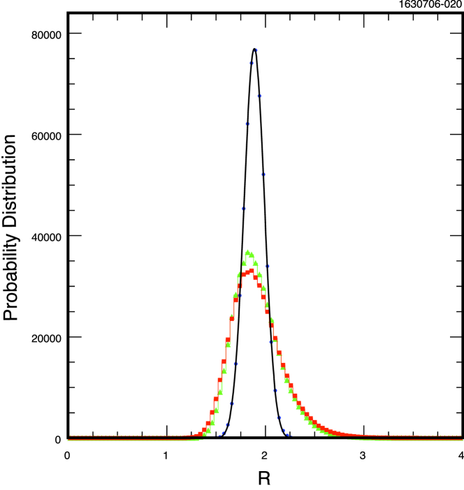
Figure 8: Probability distributions for $R$ smeared by its: (a) statistical error (solid line), (b) systematic error (filled triangles) and, (c) total error (filled squares).

We extract the statistical, systematic and total errors on our measurements from the values of these distributions corresponding to $68.3\%$ (one standard deviation) of the area under the corresponding curves (either statistical, systematic or total) above and below the maximum position. We measure

$$R=1.9\pm 0.1^{+0.3}_{-0.2}~{}.$$ (18)

II.3 Measurement of the $\Upsilon(5S)\to B_{s}^{(*)}\overline{B}_{s}^{(*)}$ Branching Fraction

Eq. (15) and the spectrum in Fig. 7 demonstrate a significant excess of $\phi$ mesons at the $\Upsilon$(5S). From these results, we can determine the fraction of the $\Upsilon$(5S) that decays into $B_{s}^{(*)}\overline{B}_{s}^{(*)}$, which we denote as $f_{S}$, in a model dependent manner. We assume that the $\phi$ yields at the $\Upsilon(5S)$ comes from two sources, $B$ and $B_{s}$ mesons. The equation linking them is

$${\cal{B}}(\Upsilon(5S)\to\phi X)/2=f_{S}\cdot{\cal{B}}(B_{s}\to\phi X)+\frac{(1-f_{S})}{2}\cdot{{\cal{B}}(\Upsilon(4S)\to\phi X)}.~{}~{}$$ (19)

We restrict our consideration to the interval $0.05<x<0.50$. We obtain $f_{S}$ via the equation correction

$$f_{S}=\frac{{\cal{B}}^{(x>0.05)}(\Upsilon(5S)\to\phi X)-{\cal{B}}^{(x>0.05)}(\Upsilon(4S)\to\phi X)}{2{\cal{B}}^{(x>0.05)}(B_{s}\to\phi X)-{\cal{B}}^{(x>0.05)}(\Upsilon(4S)\to\phi X)}~{}.$$ (20)

The branching fractions ${\cal{B}}^{(x>0.05)}(\Upsilon(5S)\to\phi X)$ and ${\cal{B}}^{(x>0.05)}(\Upsilon(4S)\to\phi X)$ are given in Eqs. 11 and 14. It is necessary to estimate ${\cal{B}}^{(x>0.05)}(B_{s}\to\phi X)$. We first show that most of the $\phi$’s in $b$ decay result from the decay chain $B\to(D$ or $D_{s})X$, $D{\rm~{}or~{}}D_{s}\to\phi X$. The decay rates for $B\to DX$ are tabulated by the PDG PDG . CLEO-c has measured, in a companion paper D_Ds_incl , the branching ratios for $D^{0}$, $D^{+}$ and $D_{s}^{+}$ mesons into $\phi$ mesons. These results are listed in the second line of Table 5.

Table 5: $B$ decay inclusive branching ratios into $D^{0}$, $D^{+}$ and $D_{s}^{+}$ mesons, the inclusive $D$ decay branching ratios into $\phi$ mesons and the resulting $B\to\phi X$ product branching ratios.

	$D^{0}$ (%)	$D^{+}$ (%)	$D_{s}^{+}$ (%)
${\cal{B}}(B\to(D$ or $D_{s})X)$	$64.0\pm 3.0$	$22.8\pm 1.4$	$8.6\pm 1.2$
${\cal{B}}((D$ or $D_{s})\to\phi X)$	$1.05\pm 0.10$	$1.03\pm 0.12$	$16.1\pm 1.6$
${\cal B}(B\to(D$ or $D_{s})X)\cdot{{\cal B}}((D$ or $D_{s})\to\phi X)$	$0.67\pm 0.08$	$0.23\pm 0.03$	$1.4\pm 0.2$

The rates on the last line of Table 5 give the resulting $\phi$ yields from the decay of $B$ into each of the individual charm mesons and the subsequent decay of the charm mesons into a $\phi$. The sum of these product rates is (2.3$\pm$0.3)%. The difference with the measured $B\to\phi X$ rate given above in Eq. (13) is an additional unaccounted for (1.2$\pm$0.4)%. This rate can be accounted for from the production of charm baryons or merely by fragmentation processes. The sum of $B\to DX$ and $D_{s}X$ branching ratios Table 5 is $(95.4\pm 3.5)$%. We now assume that the number of $D$ plus $D_{s}^{+}$ mesons produced in $B_{s}$ decays is the same as in $B$ decays. Using our previous estimate of ${\cal{B}}(B_{s}\to D_{s}X)=(92\pm 11)$% Incl_Bs_5s , we have (8$\pm$11)% of the $B_{s}$ rate into charmed mesons that must be accounted for by a mixture of $D^{0}$ and $D^{+}$, both of which have an equal decay rate into $\phi$’s. The predicted rates are

$${\cal{B}}(B_{s}\to\phi X) = (16.1\pm 2.4)\%$$ (21)

$${\cal{B}}^{(x>0.05)}(B_{s}\to\phi X) = (15.7\pm 2.3)\%,$$ (22)

where we have added in the (1.2$\pm$0.4)% from other processes; the rate for $0.05>x>0$ is taken from our Monte Carlo simulation, and amounts to 2.6% of the total yield.

Solving Eq. (20) and using our procedure for finding the errors by generating Gaussian distributions for the independent quantities leads to the probability distributions of $f_{S}$ shown in Fig. 9.

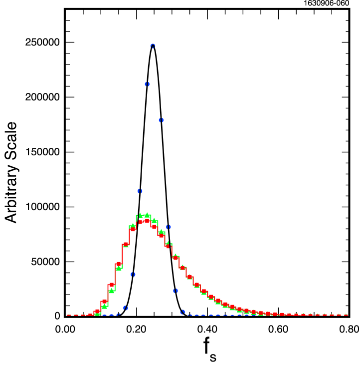
Figure 9: Probability distribution of ${\cal{B}}(\Upsilon(5S)\to B_{s}^{(*)}\overline{B}_{s}^{(*)})$, measured using the inclusive yields of $\phi$ mesons, smeared by: (a) statistical error (fitted dots), (b) systematic error (filled triangles) and, (c) total error (filled squares).

We measure the $B_{s}^{(*)}\overline{B_{s}}^{(*)}$ ratio to the total $b\overline{b}$ quark pair production above the four-flavor ($u$, $d$, $s$ and $c$ quarks) continuum background at the $\Upsilon$(5S) energy as

$${\cal{B}}(\Upsilon(5S)\to B_{s}^{(*)}\overline{B}_{s}^{(*)})=(24.6\pm 2.9^{+11.0}_{-~{}5.3})\%~{}.~{}$$ (23)

II.4 Estimate of ${\cal{B}}(\Upsilon({\rm 5S})\to\phi X)$

We estimate the branching fraction in the 0$<x<$0.05 interval for $\Upsilon$(5S) decays by using the ratio of the $\phi$ meson yield in the first $x$ interval to the total. This estimate is obtained from a combination of $B_{s}\overline{B_{s}}X$ and $B\overline{B}X$ Monte Carlo simulated decays at the $\Upsilon$(5S) energy. To combine these two types of events, we use the average of our two measurements of the $f_{S}$ fraction, 19.3%. Here the fraction in the first bin from $B$ decays is 2.4% very similar to the 2.6% from $B_{s}$ decays, that makes the error from $f_{S}$ negligible. Adding this estimate to the ${\cal{B}}^{(x>0.05)}(\Upsilon(5S)\to\phi X)=(12.9\pm 0.7^{+2.2}_{-1.4})\%$ as measured in Eq. (14), we find

$${\cal{B}}(\Upsilon(5S)\to\phi X)=(13.8\pm 0.7^{+2.3}_{-1.5})\%.~{}$$ (24)

III Updated Measurement of ${\cal{B}}(\Upsilon(5S)\to B_{s}^{(*)}\overline{B_{s}}^{(*)})$ Using $D_{s}$ Meson Yields

Here we update our measurement of $f_{s}$ using $D_{s}$ yields given in Ref. Incl_Bs_5s due to changes in the scale factors (Eqs. 6 and 7) and therefore to a better estimate of the number of hadronic events. We find the ratio

$$\frac{{\cal{B}}(\Upsilon(5S)\to D_{s}X)}{{\cal{B}}(\Upsilon(4S)\to D_{s}X)}=2.5\pm 0.2^{+0.4}_{-0.3}~{}.$$ (25)

We rewrite Eq. (19) for $D_{s}$ mesons rather than for $\phi$ mesons as

$${\cal{B}}(\Upsilon(5S)\to D_{s}X)\cdot{{\cal{B}}(D_{s}\to\phi\pi)}/2=f_{S}\cdot{\cal{B}}(B_{s}\to D_{s}X)\cdot{{\cal{B}}(D_{s}\to\phi\pi)}$$ (26)

$$+\frac{(1-f_{S})}{2}\cdot{{\cal{B}}(\Upsilon(4S)\to D_{s}X)}\cdot{{\cal{B}}(D_{s}\to\phi\pi)}~{}.~{}$$ (27)

Then using the product of production rates in Ref. Incl_Bs_5s updated with the new scale factors, our model dependent estimate of ${\cal{B}}(B_{s}\to D_{s}X)=(92\pm 11)\%$ Incl_Bs_5s and the newest estimate of ${\cal{B}}(D_{s}\to\phi\pi)=(4.4\pm 0.6)\%$ PDG , we obtain the $B_{s}^{(*)}\overline{B_{s}}^{(*)}$ ratio to the total $b\overline{b}$ quark pair production above the four-flavor ($u$, $d$, $s$ and $c$ quarks) continuum background at the $\Upsilon$(5S) energy of

$$f_{S}={\cal{B}}(\Upsilon(5S)\to B_{s}^{(*)}\overline{B}_{s}^{(*)})=(16.8\pm 2.6^{+6.7}_{-3.4})\%~{}$$ (28)

The probability distribution of this measurement within the statistical, the systematic and the total error is shown in Fig. 10.

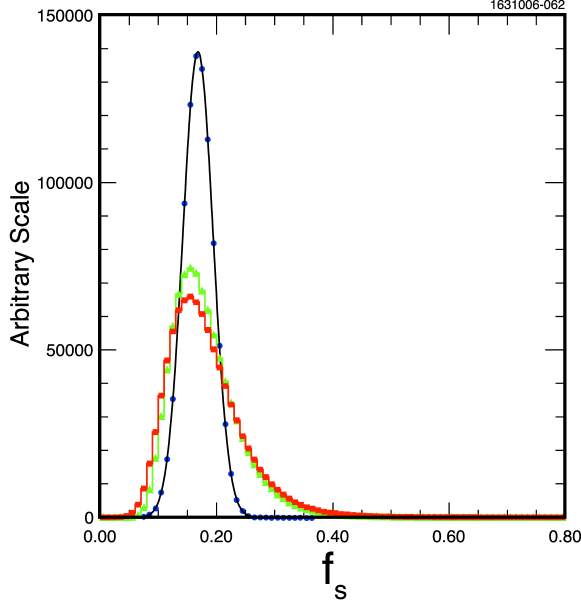
Figure 10: Probability distributions for ${\cal{B}}(\Upsilon(5S)\to B_{s}^{(*)}\overline{B}_{s}^{(*)})$, obtained by measuring $D_{s}$ yields, and smeared by: (a) statistical error (filled circles), (b) systematic error (filled triangles) and, (c) total error (filled squares).

This measurement is obtained using a value of $(4.4\pm 0.6)\%$ PDG for the $D_{s}\to\phi\pi$ branching fraction. Since this branching fraction is not well known, we show in Fig. 11 the behavior of $f_{s}$ for different values of ${\cal{B}}(D_{s}\to\phi\pi)$ ranging from $3.0$ to $5.0$%.

Figure 11: $f_{s}$ versus ${\cal{B}}(D_{s}\to\phi\pi)$ (the central line), the statistical error on $f_{s}$ is represented by the inner adjacent lines and the total error (the statistical and systematic added in quadrature) is represented by the outer two lines. The error on ${\cal{B}}(D_{s}\to\phi\pi)$ is not included.

IV The $\Upsilon(5S)$ Production Cross Section and $B$ Meson Yields

We measure the cross-section

$$\sigma(e^{+}e^{-}\to\Upsilon(5S))=(0.301\pm 0.002\pm 0.039)~{}{\rm nb}~{},$$ (29)

where the first error is statistical and the second is systematic and due to the error in the relative luminosity measurement between $\Upsilon$(5S) and continuum.

Measurement of this cross-section allows us to present the previous CLEO exclusive decay results for $B$ mesons at the $\Upsilon$(5S) B_5s in terms of branching fractions. These are given in Table 6. These results are consistent with theoretical expectations Models ; UQM .

The inclusive $B$ meson yield is represented as $B\overline{B}X$ in the Table. This measurement of ($58.9\pm 10.0\pm 9.2)$% is equal to 1-$f_{S}$ under the assumption that there are no non-$b\overline{b}$ decays of the $\Upsilon$(5S).

Table 6: Branching fractions of the possible $\Upsilon$(5S) final states either measured directly in this paper or estimated using our measurement of the $\Upsilon$(5S) total cross section and the cross section and upper limits reported in Ref. B_5s .

Different components	Measured	Corresponding
of the $\Upsilon$(5S)	cross-section (nb)	Branching Fraction ($\%$)
$B_{s}^{(*)}\overline{B}_{s}^{(*)}$	$-$	$(16.8\pm 2.6^{+6.7}_{-3.4})\%$
		(using $D_{s}$ yields)
$B_{s}^{(*)}\overline{B}_{s}^{(*)}$	$-$	$(24.6\pm 2.9^{+11.0}_{-~{}5.3})\%$
		(using $\phi$ yields)
$B\overline{B}X$	$0.177\pm 0.030\pm 0.016$	$58.9\pm 10.0\pm 9.2$
$B^{*}\overline{B}^{*}$	$0.131\pm 0.025\pm 0.014$	$43.6\pm 8.3\pm 7.2$
$B\overline{B}^{*}+B^{*}\overline{B}$	$0.043\pm 0.016\pm 0.006$	$14.3\pm 5.3\pm 2.7$
$B\overline{B}$	$<0.038$   (@ 90% CL)	$<13.8$
$B\overline{B}^{(*)}\pi+B^{(*)}\overline{B}\pi$	$<0.055$   (@ 90% CL)	$<19.7$
$B\overline{B}\pi\pi$	$<0.024$   (@ 90% CL)	$<8.9$

V Conclusions

We measure the momentum spectra of $\phi$ mesons from $\Upsilon$(4S) and $\Upsilon$(5S) decays, and use these data to estimate the ratio $f_{S}$ of $B_{s}^{(*)}\overline{B_{s}}^{(*)}$ to the total $b\overline{b}$ quark pair production at the $\Upsilon$(5S) energy as $(24.6\pm 2.9^{+11.0}_{-~{}5.3})\%$. We also update our previous measurement of $f_{S}$ using $D_{s}$ yields Incl_Bs_5s , and we find $(16.8\pm 2.6^{+6.7}_{-3.4})\%$. The central value and the error slightly change due to a better determination of the relative luminosity. Furthermore, using our cross-section measurement of $\sigma_{5S}=(0.301\pm 0.002\pm 0.039)$ nb for hadron production above 4-flavor continuum at the $\Upsilon$(5S) energy, we measure total $B$ meson production and extract $f_{S}=(41.1\pm 10.0\pm 9.2$)%. Taking a weighted average of all three methods gives $f_{S}=(21^{+6}_{-3})$%, where common systematic errors have been accounted for.

Our results as summarized in Table 7, and at the current level of precision, are consistent with the previously published phenomenological predictions Models ; UQM .

Table 7: Summary of our results.

Quantity	Measurement
Results from inclusive $\phi$ measurements
${\cal{B}}(\Upsilon(4S)\to\phi X)$	$(7.06\pm 0.09\pm 0.60)\%~{}$
${\cal{B}}(B\to\phi X)$	$(3.53\pm 0.05\pm 0.30)\%~{}$
${\cal{B}}(\Upsilon(5S)\to\phi X)$	$(13.8\pm 0.7^{+2.3}_{-1.5})\%~{}$
${{\cal{B}}(\Upsilon(5S)\to\phi X)}/{{\cal{B}}(\Upsilon(4S)\to\phi X)}$	$1.9\pm 0.1^{+0.3}_{-0.2}~{}$
${\cal{B}}(\Upsilon(5S)\to B_{s}^{(*)}\overline{B}_{s}^{(*)})$	$(24.6\pm 2.9^{+11.0}_{-~{}5.3})\%~{}$
Results from inclusive $D_{s}$ measurements
${{\cal{B}}(\Upsilon(5S)\to D_{s}X)}/{{\cal{B}}(\Upsilon(4S)\to D_{s}X)}$	$2.5\pm 0.2^{+0.4}_{-0.3}~{}$
${\cal{B}}(\Upsilon(5S)\to B_{s}^{(*)}\overline{B}_{s}^{(*)})$	$(16.8\pm 2.6^{+6.7}_{-3.4})\%~{}$
Results from cross-section and $B$ measurements
$\sigma(e^{+}e^{-}\to\Upsilon(5S))$	$(0.301\pm 0.002~{}\pm 0.039)~{}$nb
${\cal{B}}(\Upsilon(5S)\to B_{s}^{(*)}\overline{B}_{s}^{(*)})$	$(41.1\pm 10.0\pm 9.2)\%~{}$
$f_{S}$ from combining inclusive $\phi$, $D_{s}$ and $B$ measurements
${\cal{B}}(\Upsilon(5S)\to B_{s}^{(*)}\overline{B}_{s}^{(*)})$	$(21^{+6}_{-3})\%~{}$

VI Acknowledgements

We gratefully acknowledge the effort of the CESR staff in providing us with excellent luminosity and running conditions. D. Cronin-Hennessy and A. Ryd thank the A.P. Sloan Foundation. This work was supported by the National Science Foundation, the U.S. Department of Energy, and the Natural Sciences and Engineering Research Council of Canada.

References

(1)
D. Besson et al. (CLEO Collaboration), Phys. Rev. Lett. 54, 381 (1985).
(2)
D. M. Lovelock et al. (CUSB Collaboration), Phys. Rev. Lett.
54, 377 (1985).
(3)
A. D. Martin and C.-K. Ng, Z. Phys. C 40, 139 (1988); N.
Beyers and E. Eichten, Nucl. Phys. B (Proc. Suppl.) 16, 281
(1990); N. Byers, in Proceedings of the International
Conference on Quark Confinement and the Hadron Spectrum (Como,
Italy, June 1994), ed. N. Brambilla and G.M. Prosperi, World
Scientific [hep-ph/9412292] (1994).
(4)
N. A. Trnqvist, Phys. Rev. Lett. 53, 878
(1984);
S. Ono, N. A. Trnqvist, J. Lee-Franzini and A. Sanda,
Phys. Rev. Lett. 55, 2938 (1985);
S. Ono, A. Sanda and N. Trnqvist, Phys. Rev. d34, 186 (1986).
(5)
M. Artuso et al. (CLEO Collaboration), Phys. Rev. Lett. 95, 261801 (2005) [hep-ex/0508047].
(6)
G. Bonvincini et al. (CLEO Collaboration), Phys. Rev. Lett.
96, 022002 (2006) [hep-ex/0510034].
(7)
A. Drutskoy, “Results of the Engineering Run
(Belle),” [hep-ex/0605110] (2006).
(8)
O. Aquines et al. (CLEO Collaboration), Phys. Rev. Lett. 96, 152001 (2006) [hep-ex/0601044].
(9) N.G. Akeroyd et al., [hep-ex/0406071];
J.L. Hewitt and D.G. Hitlin (editors), [hep-ph/0503261].
(10)
R. Sia and S. Stone, Phys. Rev. D74, 031501 (2006)
[hep-ph/0604201].
(11)
G. S. Huang et al. (CLEO Collaboration), “Measurement of
Inclusive Production of , and Mesons in
, and Decays,” CLNS 06/1975, CLEO 06-17
[hep-ph/0610008] (2006), submitted to Phys. Rev. D.
(12)
W.-M. Yao et al., J. Phys. G33, 1 (2006).
(13) D. Peterson et al., Nucl. Instrum. and Meth. A478, 142 (2002); Y. Kubota et al. (CLEO Collaboration), Nucl.
Instrum. and Meth. A320, 66 (1992).
(14)
M. Artuso et al., Nucl. Instrum. and Meth. A554, 147 (2005);
M. Artuso et al., Nucl. Instrum. and Meth. A502, 91 (2003).
(15)
G. Fox and S. Wolfram, Phys. Rev. Lett. 41, 1581 (1978).
(16)
We ignore 1% corrections due to non-scaling changes of the
yields in the first bin.