Precise determination of the spin structure function $\mathbf{g_{1}}$
of the proton, deuteron and neutron

Abstract

Precise measurements of the spin structure functions of the proton $g_{1}^{p}(x,Q^{2})$ and deuteron $g_{1}^{d}(x,Q^{2})$ are presented over the kinematic range $0.0041\leq x\leq 0.9$ and $0.18$ GeV² $\leq Q^{2}\leq 20$ GeV². The data were collected at the HERMES experiment at DESY, in deep-inelastic scattering of 27.6 GeV longitudinally polarized positrons off longitudinally polarized hydrogen and deuterium gas targets internal to the HERA storage ring. The neutron spin structure function $g_{1}^{n}$ is extracted by combining proton and deuteron data. The integrals of $g_{1}^{p,d}$ at $Q^{2}=5$ GeV² are evaluated over the measured $x$ range. Neglecting any possible contribution to the $g_{1}^{d}$ integral from the region $x\leq 0.021$, a value of $0.330\pm 0.011\mathrm{(theo.)}\pm 0.025\mathrm{(exp.)}\pm 0.028$(evol.) is obtained for the flavor-singlet axial charge $a_{0}$ in a leading-twist NNLO analysis.

I Introduction

A major goal in the study of Quantum Chromo-Dynamics (QCD) in recent years has been the detailed investigation of the spin structure of the nucleon and the determination of the partonic composition of its spin projection:

$$S_{z}=\frac{1}{2}=\frac{1}{2}\Delta\Sigma(\mu^{2})+\Delta g(\mu^{2})+L_{z}^{q}(\mu^{2})+L_{z}^{g}(\mu^{2})\,.$$ (1)

Here $\frac{1}{2}\Delta\Sigma$ ($\Delta g$) describes the net integrated contribution of quark and anti-quark (gluon) helicities to the nucleon helicity and $L_{z}^{q}$ ($L_{z}^{g}$) is the $z$ component of the orbital angular momentum among all quarks (gluons). The individual terms in the sum are dependent on scale $\mu$ and factorization scheme, and the decomposition of the gluon total angular momentum $J^{g}_{z}(\mu^{2})=\Delta g(\mu^{2})+L_{z}^{g}(\mu^{2})$ is not gauge invariant.

Detailed information about $\Delta\Sigma$ and its flavor decomposition into the contributions from quarks and antiquarks can be obtained from various sources. In the context of this paper, double-spin asymmetries of cross sections in inclusive deep-inelastic scattering (DIS) $\ell+N\to\ell+X$ of longitudinally polarized charged leptons off longitudinally polarized nucleons are considered, where only the scattered charged lepton is observed but not the hadronic final state $X$. Inclusive scattering is sensitive to the square of the quark charges, and therefore cannot distinguish quarks from anti-quarks. This distinction can be made in semi-inclusive deep-inelastic scattering $\ell+N\to\ell+h+X$, where in addition to the scattered lepton one or more hadrons, produced in the reaction, are recorded Airapetian et al. (2005a); Adeva et al. (1998a).

The theoretical and experimental status on the spin structure of the nucleon has been discussed in great detail in several recent reviews (see, e.g., Refs. Anselmino et al. (1995); Lampe and Reya (2000); Hughes and Voss (1999); Filippone and Ji (2001); Leader (2001) and references therein). Here only the essential ingredients will be summarized.

In lowest order perturbation theory, the deep-inelastic reaction $\ell+N\to\ell+X$ proceeds via the exchange of a neutral virtual boson ($\gamma^{*},Z^{0}$). At HERMES center-of-mass energies contributions from $Z^{0}$-exchange to the cross section can be safely neglected. Therefore only the electromagnetic interaction in the approximation of one-photon exchange is taken into account here. In this approximation, the cross section of polarized inclusive DIS is parameterized by two spin structure functions $g_{1}$ and $g_{2}$. These functions cannot presently be calculated from the QCD Lagrangian.

In the QCD-improved quark parton model (QPM), i.e., at leading twist, and to leading logarithmic order in the running strong coupling constant $\alpha_{s}(Q^{2})$ of Quantum-Chromodynamics (LO QCD), the deep-inelastic scattering off the nucleon can be interpreted as the incoherent superposition of virtual-photon interactions with quarks of any flavour $q$. By angular momentum conservation, a spin-$\frac{1}{2}$ parton can absorb a hard photon only when their spin orientations are opposite. Polarized photons with the same (opposite) helicity as the polarized target nucleon consequently probe the quark number density $q_{\stackrel{{\scriptstyle\rightharpoonup}}{{\Rightarrow}}}(x,Q^{2})$ ($q_{\stackrel{{\scriptstyle\rightharpoonup}}{{\Leftarrow}}}(x,Q^{2})$) for quarks with the same (opposite) helicity as that of the parent nucleon. The spin structure function $g_{1}$ has then a probabilistic interpretation, which for the proton and the neutron reads:

$$g_{1}^{p,n}(x,Q^{2})=\frac{1}{2}\sum_{q}e^{2}_{q}\left[\Delta q^{p,n}(x,Q^{2})+\Delta\bar{q}^{p,n}(x,Q^{2})\right]$$

$$=\frac{1}{2}\langle e^{2}\rangle\left[\Delta q_{S}(x,Q^{2})+\Delta q^{p,n}_{NS}(x,Q^{2})\right].$$ (2)

Here, the quantity $-Q^{2}$ is the squared four-momentum transferred by the virtual photon, $x$ is the fraction of the nucleon’s light-cone momentum carried by the struck quark, $e_{q}$ is the charge, in units of the elementary charge $|e|$, of quarks of flavor $q$, $\langle e^{2}\rangle=\sum_{q}e^{2}_{q}/N_{q}$ is the average squared charge of the $N_{q}$ active quark flavors, and $\Delta{q}(x,Q^{2})=q_{\stackrel{{\scriptstyle\rightharpoonup}}{{\Rightarrow}}}(x,Q^{2})-q_{\stackrel{{\scriptstyle\rightharpoonup}}{{\Leftarrow}}}(x,Q^{2})$ is the quark helicity distribution for massless quarks of flavor $q$ in a longitudinally polarized nucleon in the ‘infinite-momentum frame’. Correspondingly, $\Delta{\bar{q}}(x,Q^{2}),\bar{q}_{\stackrel{{\scriptstyle\rightharpoonup}}{{\Rightarrow}}}(x,Q^{2})$ and $\bar{q}_{\stackrel{{\scriptstyle\rightharpoonup}}{{\Leftarrow}}}(x,Q^{2})$ are anti-quark distributions. The flavor singlet and flavor non-singlet quark helicity distributions are defined as

$$\Delta q_{S}(x,Q^{2}) = \sum_{q}\left[\Delta q^{p,n}(x,Q^{2})+\Delta\bar{q}^{p,n}(x,Q^{2})\right]$$ (3)

$$\equiv \Delta{\Sigma}(x,Q^{2}),$$

and

$$\Delta q_{NS}^{p,n}(x,Q^{2})\!\! = \!\!\frac{1}{\langle e^{2}\rangle}\!\sum_{q}e^{2}_{q}\left[\Delta q^{p,n}(x,Q^{2})\!+\!\Delta\bar{q}^{p,n}(x,Q^{2})\right]$$ (4)

$$-\Delta q_{S}(x,Q^{2}).$$

The functions $g_{1}^{p}$ and $g_{1}^{n}$ differ only in their non-singlet components, which through isospin symmetry are obtained from each other by exchanging $u$ and $d$ quarks: $\Delta u^{p}=\Delta d^{n}\equiv\Delta u,\Delta d^{p}=\Delta u^{n}\equiv\Delta d$. For the analysis presented in this paper, only the three lightest quark flavors, $q=u,d,s$, are taken into account and the number of active quark flavors $N_{q}$ is equal to three.

Quantities of particular importance are the first moments of the quark helicity distributions:

$$\Delta q(Q^{2})=\int_{0}^{1}\!\!\!{\rm\,d}x\,\Delta q(x,Q^{2})\,.$$ (5)

The quantity ($\Delta q(Q^{2})+\Delta{\bar{q}}(Q^{2}))$ is the net number of quarks plus antiquarks of flavor $q$ with positive helicity inside a nucleon with positive helicity and thus $\frac{1}{2}\Delta\Sigma(Q^{2})$ is the net contribution to the nucleon’s helicity that can be attributed to the helicities of the quarks.

In LO QCD the gluon distribution does not contribute explicitly in Eq. (I) to the structure function $g_{1}(x,Q^{2})$, but it does appear in the QCD evolution equations Altarelli and Parisi (1977) for $g_{1}$. Beyond leading order QCD, also gluons have to be taken explicitly into account in the expression for $g_{1}$, with $\Delta g(x,Q^{2})$ being the gluon helicity distribution. The first moment $\Delta g(Q^{2})=\int_{0}^{1}\!\!\!{\rm\,d}x\,\Delta g(x,Q^{2})$ represents the total gluon helicity contribution to the helicity of the nucleon.

If the electromagnetic currents in the nucleon are treated as fields of free quarks of only the lightest three flavors, the first moment of the structure function $g_{1}$ can be decomposed into contributions from the axial charges $a_{3},a_{8}$, and $a_{0}$, which are related to the hadronic matrix elements of the octet plus singlet quark SU(3) axial vector currents. In the scaling (Bjorken) limit,

$$\Gamma_{1}^{p,n}(Q^{2})=\int_{0}^{1}\!\!\!{\rm\,d}x\,g_{1}^{p,n}(x,Q^{2})=\frac{1}{36}\left(a_{8}\pm 3a_{3}+4a_{0}\right).$$ (6)

Here the +($-$) sign of the $a_{3}$ term holds for the proton (neutron). In the naive quark model, the axial charges are related to the first moments of quark helicity distributions by

$$a_{3}=(\Delta u+\Delta\bar{u})-(\Delta d+\Delta\bar{d}),$$ (7)

$$a_{8}=(\Delta u+\Delta\bar{u})+(\Delta d+\Delta\bar{d})-2(\Delta s+\Delta\bar{s}),$$ (8)

$$a_{0}=(\Delta u+\Delta\bar{u})+(\Delta d+\Delta\bar{d})+(\Delta s+\Delta\bar{s})\equiv\Delta\Sigma.$$ (9)

The quantities on either side of Eqs. (7) and (8) are flavor non-singlet quantities and independent of $Q^{2}$ to any order in $\alpha_{s}(Q^{2})$. Beyond LO, $a_{0}$ becomes dependent on $Q^{2}$, and $\Delta\Sigma$ may or may not be the same and may or may not depend on $Q^{2}$, depending on the factorization scheme chosen Adler (1969); Bell and Jackiw (1969).

In the approximation of SU(3) flavor symmetry and of identical masses of up-, down-, and strange-quarks, the fundamental non-singlet quantities $a_{3}$ and $a_{8}$ can be related to the two decay constants $F$ and $D$ which govern the Gamow-Teller part of the flavor-changing weak decays in the spin-$\frac{1}{2}$ baryon octet Anselmino et al. (1995): $a_{3}=F+D$ and $a_{8}=3F-D$. Here the values $F=0.464\pm 0.008$ and $D=0.806\pm 0.008$ are used as obtained from a fit to recent hyperon decay data Eidelman et al. (2004), leading to $a_{3}=F+D=g_{A}/g_{V}=1.269\pm 0.003$ and $a_{8}=3F-D=0.586\pm 0.031$, with negligible correlation between $a_{3}$ and $a_{8}$. Measurements of one of the spin structure functions $g_{1}^{p,n,d}$ and its first moment provide via Eqs. (6) to (8) the third necessary input for the determination of the flavor-singlet axial charge $a_{0}$, and thereby also of $\Delta{\Sigma}$ and the moments of the helicity distributions of the three quark flavors ($\Delta u+\Delta\bar{u}$), ($\Delta d+\Delta\bar{d}$) and ($\Delta s+\Delta\bar{s}$).

At any order in $\alpha_{s}(Q^{2})$ and in a leading-twist approximation, the structure function $g_{1}$ is a convolution of quark, anti-quark and gluon helicity distributions Altarelli et al. (1997) with Wilson coefficient functions $\Delta C(x,\alpha_{s}(Q^{2}))$ Mertig and van Neerven (1996):

$$g_{1}^{p,n}(x,Q^{2})=\\ \displaystyle\frac{1}{2}\langle e^{2}\rangle\int_{x}^{1}\frac{\mathrm{d}x^{\prime}}{x^{\prime}}\left[\Delta C_{S}\left(\frac{x}{x^{\prime}},\alpha_{s}(Q^{2})\right)\Delta q_{S}(x^{\prime},Q^{2})\right.\\ +\left.2N_{q}\Delta C_{g}\left(\frac{x}{x^{\prime}},\alpha_{s}(Q^{2})\right)\Delta g(x^{\prime},Q^{2})\right.\\ +\left.\Delta C_{NS}^{p,n}\left(\frac{x}{x^{\prime}},\alpha_{s}(Q^{2})\right)\Delta q_{NS}^{p,n}(x^{\prime},Q^{2})\right].$$ (10)

In LO Eq. (10) reduces to Eq. (I) since then $\Delta C_{S}$ and $\Delta C_{NS}$ become $\delta$ functions and $\Delta C_{g}$ vanishes. The factorization between the helicity distributions and the coefficient functions involves some arbitrary choice, and hence the distributions and their moments depend on the factorization scheme. The structure function $g_{1}(x,Q^{2})$, as a physical observable, is scheme independent. There are straightforward transformations that relate different schemes and their results to each other. In the ‘modified minimal subtraction’ ($\overline{MS}$) scheme Bardeen (1978), the factorization scheme commonly used in most of the present NLO analyses of unpolarized deep-inelastic and hard processes, the first moment of the gluon coefficient function vanishes and $\Delta{g}(Q^{2})$ does not contribute to the first moment of $g_{1}$. Therefore $\Gamma_{1}$ can be directly related to $a_{0}(Q^{2})\stackrel{{\scriptstyle\scriptstyle\overline{MS}}}{{=}}\Delta{\Sigma}(Q^{2})$.

In the $\overline{MS}$ scheme, Eq. (6) becomes

$$\Gamma_{1}^{p,n}(Q^{2}) = \frac{1}{36}\left[(a_{8}\pm 3a_{3})\Delta C_{NS}^{\overline{MS}}(\alpha_{s}(Q^{2}))\right.$$ (11)

$$\left.+4a_{0}\Delta C_{S}^{\overline{MS}}(\alpha_{s}(Q^{2}))\right],$$

where $\Delta C_{NS}^{\overline{MS}}(\alpha_{s}(Q^{2}))$ and $\Delta C_{S}^{\overline{MS}}(\alpha_{s}(Q^{2}))$ are the first moments of the non-singlet and singlet Wilson coefficient functions, respectively.

The difference of the $g_{1}$ moments for proton and neutron leads to the Bjorken Sum Rule Bjorken (1966, 1970), which in leading twist reads:

$$\Gamma_{1}^{p}(Q^{2})-\Gamma_{1}^{n}(Q^{2})=\frac{1}{6}a_{3}\Delta C_{NS}^{\overline{MS}}(\alpha_{s}(Q^{2})),$$ (12)

while their sum is given by:

$$\Gamma_{1}^{p}(Q^{2})+\Gamma_{1}^{n}(Q^{2}) = \frac{1}{18}\left[a_{8}\Delta C_{NS}^{\overline{MS}}(\alpha_{s}(Q^{2}))\right.$$ (13)

$$\left.+4a_{0}\Delta C_{S}^{\overline{MS}}(\alpha_{s}(Q^{2}))\right].$$

This sum equals twice the deuteron moment apart from a small correction due to the D-wave admixture to the deuteron wave function (see Eq. (23)). The measurement of $\Gamma_{1}^{d}$ hence allows for a straightforward determination of $a_{0}$ using only $a_{8}$ as additional input.

In the $\overline{MS}$ scheme, the non-singlet (singlet) coefficient has been calculated up to third (second) order in the strong coupling constant Larin and Vermaseren (1991):

$$\Delta C_{NS}^{\overline{MS}}(\alpha_{s}(Q^{2}))\! = \!1-\!\frac{\alpha_{s}}{\pi}\!-\!3.583\left(\frac{\alpha_{s}}{\pi}\right)^{2}\!\!-\!20.215\left(\frac{\alpha_{s}}{\pi}\right)^{3}$$ (14)

$$\Delta C_{S}^{\overline{MS}}(\alpha_{s}(Q^{2})) = 1-\left(\frac{\alpha_{s}}{\pi}\right)-1.096\left(\frac{\alpha_{s}}{\pi}\right)^{2},$$ (15)

for $N_{q}=3$ Larin et al. (1997). Estimates exist for the fourth (third) order non-singlet (singlet) term Kataev and Starshenko (1995).

The first determination of $\Delta\Sigma$ was a moment analysis of the EMC proton data Ashman et al. (1988), using Eq. (11) and the moments of the Wilson coefficients in $\mathcal{O}(\alpha_{s}^{1})$. It resulted in $\Delta\Sigma=0.120\pm 0.094\mathrm{(stat)}\pm 0.138$(sys), much smaller than the expectation ($\Delta\Sigma\approx 0.6$) Jaffe and Manohar (1990); Schreiber and Thomas (1988) from the relativistic constituent quark model. This result caused enormous activity in both experiment and theory. A series of high-precision scattering experiments with polarized beams and targets were completed at CERN Adeva et al. (1999, 1997, 1998b), SLAC Abe et al. (1998); Anthony et al. (1999a, 2000a), DESY Ackerstaff et al. (1997) and continue at CERN Ageev et al. (2005) and JLAB Zheng et al. (2004). Such measurements are always restricted to certain $x$ and $Q^{2}$ ranges due to the experimental conditions. However, any determination of $\Delta\Sigma$ requires an ‘evolution’ to a fixed value of $Q^{2}$ and an extrapolation of $g_{1}$ data to the full $x$ range and substantial uncertainties might arise from the necessary extrapolations $x\rightarrow 0$ and $x\rightarrow 1$. This limitation applies also to recent determinations of $\Delta\Sigma$ based on NLO fits Abe et al. (1997a); Adeva et al. (1998c); Goto et al. (2000); Glück et al. (2001); Blümlein and Böttcher (2002) of the $x$ and $Q^{2}$ dependence of $g_{1}$ for proton, deuteron, and neutron, using Eq. (10) and the corresponding evolution equations.

This paper reports final results obtained by the HERMES experiment on the structure function $g_{1}$ for the proton, deuteron, and neutron. The results include an analysis of the proton data collected in 1996, a re-analysis of 1997 proton data previously published Airapetian et al. (1998), as well as the analysis of the deuteron data collected in the year 2000. While the accuracy of the HERMES proton data is comparable to that of earlier measurements, the HERMES deuteron data are more precise than all published data. By combining HERMES proton and deuteron data, precise results on the neutron spin structure function $g_{1}^{n}$ are obtained.

For this analysis, the kinematic range has been extended with respect to the previous proton analysis, to include the region at low $x$ ($0.0041\leq x\leq 0.0212$) with low $Q^{2}$. In this region the information available on $g_{1}$ was sparse. As will be discussed in Sect. VI, the first moment $\Gamma_{1}^{d}$ determined from HERMES data appears to saturate for $x<0.04$. This observation allows for a determination of $a_{0}$ with small uncertainties and for a test of the Bjorken Sum Rule, as well as scheme-dependent estimates of $\Delta\Sigma$ and the first moments of the flavor separated quark helicity distributions, $\Delta u+\Delta\bar{u}$, $\Delta d+\Delta\bar{d}$ and $\Delta s+\Delta\bar{s}$.

The paper is organized as follows: the formalism leading to the extraction of the structure function $g_{1}$ will be briefly reviewed in Sect. II, Sect. III deals with the HERMES experimental arrangement and the data analysis is described in Sect. IV. Final results are presented in Sect. V and discussed in Sect. VI.

II Formalism

In the one-photon-exchange approximation, the differential cross section for inclusive deep-inelastic scattering of polarized charged leptons off polarized nuclear targets can be written Leader and Predazzi (1982) as:

$$\frac{\mathrm{d}^{2}\sigma(s,S)}{\mathrm{d}x~{}\mathrm{d}Q^{2}}=\frac{2\pi\alpha^{2}y^{2}}{Q^{6}}{{\mathbf{L_{\mu\nu}}(s)\mathbf{W^{\mu\nu}}(S)}}\,,$$ (16)

where $\alpha$ is the fine-structure constant. As depicted in Fig. 1 the leptonic tensor $\mathbf{L_{\mu\nu}}$ describes the emission of a virtual photon at the lepton vertex, and the hadronic tensor $\mathbf{W^{\mu\nu}}$ describes the hadron vertex. The main kinematic variables used for the description of deep-inelastic scattering are defined in Tab. 1.

Figure 1: Schematic picture of Deep-Inelastic Scattering for one photon exchange. The kinematic variables are defined in Tab. 1.

The tensor $\mathbf{L_{\mu\nu}}$ can be calculated precisely in Quantum Electro-Dynamics (QED) Bjorken (1970):

$$\mathbf{L_{\mu\nu}}(s) = 2(k_{\mu}k^{\prime}_{\nu}+k_{\nu}k^{\prime}_{\mu}-g_{\mu\nu}(k\cdot k^{\prime}-m^{2}_{l}))$$ (17)

$$+ 2i\epsilon_{\mu\nu\alpha\beta}(k-k^{\prime})^{\alpha}s^{\beta}\,.$$

Here the spinor normalization $s^{2}=-m_{l}^{2}$ is used. In the following the lepton mass $m_{l}$ is neglected. For a spin-1/2 target the representation of $\mathbf{W^{\mu\nu}}$ requires four structure functions to describe the nucleon’s internal structure. It can be written as Bjorken (1970); Close (1979); Hughes and Kuti (1983):

$$\!\!\!\!\!\!\!{\mathbf{W^{\mu\nu}_{\frac{1}{2}}}}(S)\!\!\! = \!\!\left(-g^{\mu\nu}-\frac{q^{\mu}q^{\nu}}{Q^{2}}\right)F_{1}$$ (18)

$$+ \!\!\left(P^{\mu}+\frac{P\cdot q}{Q^{2}}q^{\mu}\right)\left(P^{\nu}+\frac{P\cdot q}{Q^{2}}q^{\nu}\right)\frac{F_{2}}{P\cdot q}$$

$$- \!\!\!i\epsilon^{\mu\nu\lambda\sigma}\frac{q_{\lambda}}{P\cdot q}\left[S_{\sigma}g_{1}+\!\left(S_{\sigma}\!-\frac{S\cdot q}{P\cdot q}P_{\sigma}\right)\!g_{2}\right]\!\!.$$

Here, $F_{1}$ and $F_{2}$ are polarization-averaged structure functions (in the following also called ’unpolarized’), while $g_{1}$ and $g_{2}$ are spin structure functions, all depending on both $x$ and $Q^{2}$, which have been suppressed here for simplicity. The sensitivity of the cross section to $g_{1}$ and $g_{2}$ arises from the product of the anti-symmetric parts of the $\mathbf{L_{\mu\nu}}$ and $\mathbf{W^{\mu\nu}}$ tensors, which is non-zero only when both target and beam are polarized.

Table 1: Kinematic variables used in the description of deep-inelastic scattering.

$m_{l}$	Mass of incoming lepton (considered as negligible)
$M$	Mass of target nucleon
$k=(E,\vec{k})$, $k^{\prime}=(E^{\prime},\vec{k^{\prime}})$	4–momenta of the initial and final state leptons
$s$, $S$	Lepton’s and target’s spin 4-vectors
$\theta,\;\phi$	Polar and azimuthal angle of the scattered lepton
$P\stackrel{{\scriptstyle\mathrm{lab}}}{{=}}(M,0)$	4–momentum of the initial target nucleon
$q=(E-E^{\prime},\vec{k}-\vec{k^{\prime}})$	4–momentum of the virtual photon
$Q^{2}=-q^{2}$ $\stackrel{{\scriptstyle\mathrm{lab}}}{{\approx}}4EE^{\prime}\sin^{2}\frac{\theta}{2}$	Negative squared 4–momentum transfer
$\displaystyle{\nu=\frac{P\cdot q}{M}\stackrel{{\scriptstyle\mathrm{lab}}}{{=}}E-E^{\prime}}$	Energy of the virtual photon in the target rest frame
$\displaystyle{x=\frac{Q^{2}}{2\,P\cdot q}=\frac{Q^{2}}{2\,M\nu}}$	Bjorken scaling variable
$\displaystyle{y=\frac{P\cdot q}{P\cdot k}=\frac{\nu}{E}}$
$W^{2}=(P+q)^{2}$ $=M^{2}+2M\nu-Q^{2}$	Squared invariant mass of the photon–nucleon system

For a spin-1 target such as the deuteron, the hadronic tensor has four additional structure functions arising from its electric quadrupole structure Hoodbhoy et al. (1989); Sather et al. (1990). Only three appear at leading-twist level: $b_{1}$, $b_{2}$ and $\Delta$. In the scaling (Bjorken) limit the structure function $b_{2}$ is related to $b_{1}$ by $b_{2}(x)=2xb_{1}(x)$; $\Delta$ describes the double helicity-flip (virtual) photon-deuteron amplitude Jaffe et al. (1989). The structure function $b_{1}$ appears in a product with the tensor polarization of the target, which can coexist with the vector polarization in spin-1 targets. The influence of the tensor polarization on the $g_{1}$ measurement is discussed in Sect. C. In this analysis the unmeasured function $\Delta$ is neglected since its contribution is suppressed for longitudinally polarized targets.

The structure function $g_{1}$ is related directly to the cross section difference:

$$\sigma_{LL}\equiv\frac{1}{2}(\sigma^{\stackrel{{\scriptstyle\rightarrow}}{{\Leftarrow}}}-\sigma^{\stackrel{{\scriptstyle\rightarrow}}{{\Rightarrow}}})\,,$$ (19)

where longitudinally ($L$) polarized leptons ($\rightarrow$) scatter on longitudinally ($L$) polarized nuclear targets with polarization direction either parallel or anti-parallel (${\stackrel{{\scriptstyle\rightarrow}}{{\Rightarrow}}}$, ${\stackrel{{\scriptstyle\rightarrow}}{{\Leftarrow}}}$) to the spin direction of the beam. The relationship to spin structure functions is:

$$\frac{{\rm\,d^{2}\!}\sigma_{LL}(x,Q^{2})}{{\rm\,d}x{\rm\,d}Q^{2}}=\frac{8\pi\alpha^{2}y}{Q^{4}}\\ \times\left[\left(1-\frac{y}{2}-\frac{y^{2}}{4}\gamma^{2}\right)\,g_{1}(x,Q^{2})-\frac{y}{2}\gamma^{2}\,g_{2}(x,Q^{2})\right]\,,$$ (20)

where $\gamma^{2}=Q^{2}/\nu^{2}$. The spin structure function $g_{2}(x,Q^{2})$ does not have any probabilistic interpretation in the QPM. It will not be discussed further in this paper, but it is taken into account in the extraction of $g_{1}$ by using a parameterization of the published data. The second term is small compared to the first. Averaged over all $(x,Q^{2})$ bins of this analysis it is of order 0.54$\%$ for the proton and 1.9$\%$ for the deuteron. Therefore the existing precision for $g_{2}$ has only a marginal effect on an extraction of $g_{1}$.

For only the purely technical reason that absolute cross sections are difficult to measure, asymmetries are the usual direct experimental observable:

$$A_{||}\equiv\frac{\sigma_{LL}}{\sigma_{UU}}\,,$$ (21)

where $\sigma_{UU}$ is the polarization-averaged cross section, wherein the subscript $UU$ indicates that both beam and target are unpolarized. Parity conservation implies $\sigma_{UU}=\sigma_{LU}\equiv\frac{1}{2}(\sigma^{\stackrel{{\scriptstyle\rightarrow}}{{\Leftarrow}}}+\sigma^{\stackrel{{\scriptstyle\rightarrow}}{{\Rightarrow}}})$. Values of absolute polarization-averaged DIS cross sections $\sigma_{UU}$ are introduced from previous experiments that were designed to measure them precisely. These cross sections are all that is needed to extract the spin structure function $g_{1}$ at the measured combinations of $x$ and $Q^{2}$. They are also needed in the process of correcting the measured asymmetry $A_{||}^{m}$ for higher order QED (radiative) effects to obtain the asymmetry $A_{||}$ at Born level. This is because the polarization-averaged yields must be normalized to known values of $\sigma_{UU}$ in order to subtract QED radiative background calculated as absolute cross sections.

Substituting $\sigma_{LL}=\sigma_{UU}A_{||}$ into Eq. (20), and solving for $g_{1}$, we obtain

$$g_{1}(x,Q^{2})=\frac{1}{1-\frac{y}{2}-\frac{y^{2}}{4}\gamma^{2}}\\ \times\left[\frac{Q^{4}}{8\pi\alpha^{2}y}\frac{{\rm\,d^{2}\!}\sigma_{UU}(x,Q^{2})}{{\rm\,d}x{\rm\,d}Q^{2}}A_{||}(x,Q^{2})+\frac{y}{2}\gamma^{2}\,g_{2}(x,Q^{2})\right]\,.$$ (22)

The structure functions $g_{1}^{p}$ and $g_{1}^{n}$ on proton and neutron targets are related to that of the deuteron by the relation:

$${{{g_{1}^{d}}}}~{}=~{}\frac{1}{2}({{{g_{1}^{p}}}}+{{{g_{1}^{n}}}})\left(1-\frac{3}{2}\omega_{D}\right)\,,$$ (23)

where $\omega_{D}$ takes into account the D-state admixture to the deuteron wave function. A value of $\omega_{D}=0.05\pm 0.01$ is used, which covers most of the available estimates Lacombe et al. (1981); Buck and Gross (1979); Zuilhof and Tjon (1980); Machleidt et al. (1987); Umnikov et al. (1994). In this paper the neutron structure function $g_{1}^{n}$ is evaluated according to Eq. (23).

Alternatively, $g_{1}^{n}$ can be obtained, e.g., from measurements on a polarized ³He target:

$$g_{1}^{{}^{3}\textrm{He}}\simeq P_{n}g_{1}^{n}+2P_{p}g_{1}^{p}\,,$$ (24)

where the effective polarizations of neutron and proton are $P_{n}=0.86\pm 0.02$ and $P_{p}=-0.028\pm 0.004$ Ciofi degli Atti et al. (1993); i.e., the polarized ³He acts effectively as a polarized neutron target. The HERMES measurement of $g_{1}^{n}$ off ³He has been previously published in Ackerstaff et al. (1997).

III The Experiment

The HERA facility at DESY comprises a proton and a lepton storage ring. HERMES is a fixed-target experiment using exclusively the lepton ring, which can be filled with either electrons or positrons (only positron data are used for this analysis), while the proton beam passes through the non-instrumented horizontal mid-plane of the spectrometer. Internal to the lepton ring, an open-ended storage cell is installed that can be fed with either polarized or unpolarized target gas. The three major components to the HERMES experiment (beam, target, spectrometer) are briefly described in the following, while detailed descriptions can be found elsewhere (Ackerstaff et al. (1998); Bernreuther et al. (1998); Avakian et al. (1998); Andreev et al. (2001); Brack et al. (2001); Benisch et al. (2001); Akopov et al. (2002); Airapetian et al. (2005b); Barber et al. (1995); Beckmann et al. (2002)).

A Polarized HERA Beam

Spin rotators and polarimeters are essential components of the HERA lepton beam. They are described in detail in Refs. Buon and Steffen (1986); Barber et al. (1993, 1994); Beckmann et al. (2002). The initially unpolarized beam becomes transversely polarized by an asymmetry in the emission of synchrotron radiation associated with a spin flip (Sokolov-Ternov mechanism Sokolov and Ternov (1964)). The beam polarization grows and approaches asymptotically an equilibrium value, with a time constant depending on the characteristics of the ring, typically over 30-40 minutes. The transverse guide field generates transverse beam polarization in the ring, while spin rotators in front of and behind the experiment provide longitudinal polarization at the interaction point and at one of the two beam polarimeters.

The two HERA beam polarimeters are based on Compton back-scattering of circularly polarized laser light. The transverse beam polarization at the opposite side of the ring causes an up-down asymmetry in the direction of the back-scattered photons. The resulting position asymmetry is measured by the top and bottom halves of the lead-scintillator sampling calorimeter of the transverse polarimeter Barber et al. (1993), with fractional systematic uncertainties of 3.5% (1996-97 data). The longitudinal beam polarization in the region of the experiment leads to an asymmetry in the energy of the back-scattered Compton photons measured in the NaBi(WO₄)₂ crystal calorimeter of the longitudinal polarimeter Beckmann et al. (2002), with fractional systematic uncertainties of 1.6% (2000 data). The average beam polarization was typically larger than 0.5.

In order to account for the time dependence of the beam polarization, its continuously monitored values are used in the analysis. The average values of the beam polarizations for each year covered in this paper are shown in Tab. 2. The numbers are weighted by the luminosity so that the value near the beginning of each fill dominates.

Table 2: Average value and uncertainty of the beam polarization for each year of measurements.

Year	Average Polarization
1996		$0.528\pm 0.018$
1997		$0.531\pm 0.018$
2000		$0.533\pm 0.010$

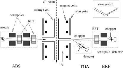
Figure 2: Schematic view of the longitudinally polarized target. From left to right: Atomic Beam Source (ABS) containing Radio-Frequency Transitions (RFT), target chamber with cell and magnet, diagnostic system composed by Target Gas Analyzer (TGA), and Breit-Rabi Polarimeter (BRP).

B The HERMES Polarized Gas Target

The combination of a fixed target with the HERA lepton storage ring requires the employment of a gaseous target internal to the beam line. This has the advantages of being almost free of dilution (the fraction $f$ of polarizable nucleons being close to 1), of providing a high degree of vector polarization ($P_{z}>0.8$), and of being able to invert the direction of the spin of the nucleons within milliseconds.

The HERMES longitudinally polarized gas target Airapetian et al. (2005b), schematically shown in Fig. 2, consists of an Atomic Beam Source (ABS) Baumgarten et al. (2003a) which produces a polarized jet of atomic hydrogen or deuterium and focuses it into a thin-walled storage cell along the beam line Baumgarten et al. (2003b). The atomic gas is produced in a dissociator and is formed into a beam using a cooled nozzle, collimators and a series of differential pumping stations. A succession of magnetic sextupoles and radio-frequency fields are used to select (by Stern-Gerlach separation) and exchange (by radio-frequency transitions) the atomic hyperfine states that have a given nuclear polarization to be injected into the cell. The storage cell, inside the HERA beam pipe, is a windowless 40 cm long elliptical tube, coaxial to the beam, with 75 $\rm\mu m$ thick Al walls coated to inhibit surface recombination and depolarization. The use of the storage cell technique results in a typical areal density increase of about two orders of magnitude compared to a free jet target. A sample of gas (ca. 5$\%$) diffuses from the middle of the cell into a Breit-Rabi Polarimeter (BRP) Baumgarten et al. (2002) which measures the atomic polarization, or into a Target Gas Analyzer (TGA) Baumgarten et al. (2003c) which measures the atomic and the molecular content of the sample. A magnet surrounding the storage cell provides a holding field defining the polarization axis and prevents spin relaxation via spin exchange or wall collisions by effectively decoupling the magnetic moments of electrons and nucleons. A gaseous helium cooling system keeps the cell temperature at the lowest value for which atomic recombination and spin relaxation during wall collisions are minimal.

The vector polarization $P_{z}$ is defined as $P_{z}\equiv(n^{+}-n^{-})/(n^{+}+n^{-})$ and $P_{z}\equiv(n^{+}-n^{-})/(n^{+}+n^{-}+n^{0})$ for spin-1/2 and spin-1 targets, respectively. Here $n^{+}$, $n^{-}$ and $n^{0}$ are the atomic populations with positive, negative and zero spin projection on the beam direction. The sign of the target polarization is randomly chosen each 60 s for hydrogen and 90 s for deuterium. The target parameters are measured for each such interval. The rapid cycling of the target polarization reduces the systematic uncertainty in the measured spin asymmetries related to the stability of the experimental setup. Due to the very stable performance of the target operation, luminosity-average polarization values are used in the analysis.

Hydrogen data
During the years 1996-97 a longitudinally polarized hydrogen target was employed at a nominal temperature $T_{cell}=100\,$K. The average target polarization for the year 1997 reached the value $P_{z}^{+}=P_{z}^{-}=0.851\pm 0.032$; the average target areal density was determined to be $7.6\cdot 10^{13}$ nucleons/cm². The target polarization for the year 1996, which contributes only about 27$\%$ to the total statistics, was determined from the normalization of the 1996 inclusive asymmetry to that of 1997. For this limited data-set this method provides a smaller uncertainty on the target polarization w.r.t. the direct measurement. In 1997, a set of data at higher temperature ($T_{cell}=260$ K) was collected in order to measure the polarization of the recombined molecules Airapetian et al. (2004), thus reducing the systematic uncertainty on the target polarization measurement by a factor close to 2.

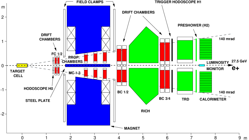
Figure 3: A schematic side view of the HERMES spectrometer.

Deuterium data
From the end of 1998 till the end of 2000 deuterium was used as target material. The data taken in 1998 and 1999 have been excluded from the present analysis because of the overwhelming statistics of the 2000 data. In the year 2000 a target cell with smaller cross section was installed with reduced nominal temperature $T_{cell}=60\,$K, thus increasing the target density by a factor of 2. The average values of the target vector polarization were $P_{z}^{+}=0.851\pm 0.031$ and $P_{z}^{-}=0.840\pm 0.028$. The two polarization values are due to different injection efficiencies of the ABS. The average target areal density was determined to be $2.1\cdot 10^{14}$ nucleons/cm². In a dedicated running period, about 3.5 million deep-inelastic scattering events were taken with tensor polarization, allowing the first measurement ever of the tensor structure function $b_{1}^{d}$ and the first assessment of the effect on the $g_{1}^{d}$ measurement by the coexistent tensor polarization of the deuteron target (see Sect. C).

Tab. 3 shows the average polarizations of the target and their uncertainties for the three data sets used in this analysis. The uncertainties are dominated by systematics, which depend on varying running conditions and quality of the target cell surface.

Table 3: Average magnitude of the target vector polarization $P_{z}$ for the various data sets.

Year	Target gas	Sign of $P_{z}$	$|P_{z}|$
1996	H	$\pm$	$0.759$ $\pm$ $0.032$
1997	H	$\pm$	$0.851$ $\pm$ $0.032$
2000	D	$+$	$0.851$ $\pm$ $0.031$
2000	D	$-$	$0.840$ $\pm$ $0.028$

C The HERMES Spectrometer

A detailed description of the HERMES spectrometer (see Fig. 3) is given in Ref. Ackerstaff et al. (1998). It constitutes a forward spectrometer with multiple tracking stages before and after a 1.5 Tm dipole magnet, and good particle identification (PID) capabilities. A horizontal iron plate shields the HERA beam lines from the dipole field, thus dividing the spectrometer in two identical halves, top and bottom. The geometrical acceptance of $\pm 170$ mrad horizontally and $\pm(40-140)$ mrad vertically results in detected scattering angles ranging from 40 to 220 mrad.

In each spectrometer half, the intersection points of charged particle trajectories with the 36 planes of the Front Chambers (FC 1-2) and Back Chambers (BC 1-4) are used for track reconstruction in space. These detectors are horizontal-drift chambers with alternating cathode and anode wires between two cathode foils, all operated with the gas mixture Ar:CO₂:CF₄ (90:5:5), the average drift velocity being 7 cm/$\mu s$. They are assembled in modules of six layers in three coordinate doublets ($XX^{\prime},UU^{\prime}$, and $VV^{\prime}$), where the primed planes are offset by half a cell width to help resolve left-right ambiguities. The cell width is 7 mm for FCs Brack et al. (2001), while it is 15 mm for BCs Bernreuther et al. (1998) behind the magnet.

The proportional wire chambers MC1-3, also shown in Fig. 3, are not included in the tracking algorithm Ackerstaff et al. (1998) used for this analysis.

This tracking algorithm determines partial tracks before (front track) and after the magnet (back track). The track projections are found in a fast tree search and then combined to determine the particle momentum. The algorithm uses the intersection point of the back track with the magnet mid-plane to refine front tracks. From their scattering angles and positions the event vertex is determined, while the back tracks are also used to identify hits in the PID detectors. Monte Carlo simulations show that the intrinsic momentum resolution $\Delta p/p$ is between 0.015 and 0.025 over the accessible momentum range. The resolution for hydrogen was better than for deuterium as the RICH detector installed before the deuterium data taking period introduced some additional material.

The scattered positron is identified through a combination of a lead-glass calorimeter, a pre-shower detector, a Transition-Radiation Detector (TRD), and the Čerenkov detectors. (While the threshold Čerenkov was used in 1996-97 primarily for pion identification, the Ring-Imaging Čerenkov (RICH) detector Akopov et al. (2002); Aschenauer et al. (2000) was used thereafter to identify pions, kaons, and protons.)

The Calorimeter Avakian et al. (1998) is used to suppress hadrons by a factor of 10 at the trigger level and a factor of 100 in the off-line analysis, to measure the energy of electrons/positrons and also of photons. Each half consists of 42x10 blocks of radiation-resistant F101 lead glass Avakian et al. (1996). Each block has a cross section of 9x9 cm² and 50 cm depth, and is viewed from the back by a photo-multiplier tube. The calorimeter’s resolution was measured to be $\sigma(E)/E[\%]=(5.1\pm 1.1)/\sqrt{E[GeV]}+(2.0\pm 0.5)+(10.0\pm 2.0)/E$ Avakian et al. (1998).

The scintillator hodoscope H2, consisting of 42 vertical 9.3x91 cm² ‘paddles’ of 1 cm thickness, forms the pre-shower detector in combination with two radiation lengths of lead preceding it. As pions deposit only about 2 MeV in H2, as compared to 20-40 MeV for leptons, the pion contamination can be reduced by more than a factor of 10 with 95% efficiency if this detector were used alone.

The TRD rejects hadrons by a factor of more than 100 at 90% electron/positron efficiency, if used alone. A TRD half comprises six proportional wire chambers to detect the photons from transition radiation in the preceding radiator. All TRD proportional chambers use Xe:CH₄ (90:10) gas.

The luminosity monitor Benisch et al. (2001) detects in coincidence $e^{+}e^{-}$ pairs originating from Bhabha scattering of the beam positrons off electrons from the target atoms, and also $\gamma\gamma$ pairs from $e^{+}e^{-}$ annihilations. It consists of two small calorimeters made of highly radiation resistant NaBi(WO₄)₂ crystals covering a horizontal acceptance of 4.6-8.9 mrad. They are mounted to the right and left of the beam pipe, 7.2 m downstream of the target.

IV Data Analysis

The inclusive data sample is selected from the recorded events to satisfy the following criteria:

• there exists a trigger composed of signals in the Calorimeter and in the hodoscopes H0, H1 and Pre-Shower (H2) (see Fig. 3),

• data quality criteria are met,

• the particles identified by the Particle Identification scheme as leptons are selected,

• the highest momentum lepton in the event originating from the target region is selected,

• geometric and kinematic constraints are applied.

A The kinematic range

The kinematic range of the events selected for this analysis is shown in Fig. 4, together with the requirements imposed on the kinematic variables.

Figure 4: Kinematic $x-Q^{2}$ and $x-y$ planes covered by this analysis. The symbols represent the average values of $(x,Q^{2})$ (top panel) and $(x,y)$ (bottom panel) in each bin. Subdivision of the $x$-bins along $Q^{2}$ is denoted by different symbols (A, B, C).

The aperture of the spectrometer limits the acceptance to scattering angles $0.04\leq\theta\leq 0.22$ mrad. The constraint $y>0.1$ is used to exclude regions where the momentum resolution starts to degrade Ackerstaff et al. (1998). The constraint $y\leq 0.91$ discards the low momentum region ($E<2.5$ GeV) where the trigger efficiencies have not yet reached a momentum plateau. The requirement $W^{2}>(1.8)^{2}$ GeV² suppresses the region of baryon resonances. The resulting ($x,Q^{2}$) region, defined by $0.0041\leq x\leq 0.9$ and $0.18$ GeV² $\leq Q^{2}\leq 20$ GeV², was divided into 19 bins in $x$, guided by the available statistics. Furthermore most $x$-bins are subdivided into up to 3 bins in $Q^{2}$, designated A, B and C bins. The purpose of this is to allow appropriate statistical weighting of these $Q^{2}$ bins, thereby exploiting the higher figure of merit at larger $Q^{2}$, which is due to both the larger polarization transfer from the incident lepton to the virtual photon, and the smaller kinematic smearing between $x$ bins. Logarithmically equidistant bin boundaries are used along the $x$ axis in the region $0.044<x<0.66$, and along the $Q^{2}$ axis in the region $x>0.06$.

B Particle Identification

The lepton (positron and electron) identification is achieved with a probability analysis based on the responses of the TRD, the pre-shower detector, the Calorimeter, and the Čerenkov detectors, described in Sect. C.

The requirement used to identify a lepton is:

$$PID=\log_{10}\frac{P(l|{\cal R},p,\theta)}{P(h|{\cal R},p,\theta)}\,>\,{PID}_{cut},$$ (25)

where $P(l(h)|{\cal R},p,\theta)$ is the conditional probability that the particle is a lepton $l$ or a hadron $h$, given the combined response set $\cal R$ from all the Particle Identification detectors, the momentum $p$, and the scattering angle $\theta$. Bayes’ theorem relates $P(l(h)|{\cal R},p,\theta)$ to the probability $P(l(h)|p,\theta)$ that a particle with momentum $p$, scattered at polar angle $\theta$, is a lepton (hadron), and the probability $P({\cal R}|l(h),p)$ that a lepton (hadron) with momentum $p$ causes the combined signal ${\cal R}$. The $PID$ can be re-written as:

$$PID\!=\log_{10}\frac{P({\cal R}|l,p)}{P({\cal R}|h,p)}\cdot\frac{P(l|p,\theta)}{P(h|p,\theta)}=PID^{\prime}-\log_{10}\Phi(p,\theta).$$ (26)

Here $\Phi(p,\theta)$ is the ratio between the hadron and lepton fluxes impinging onto the detector:

$$\Phi(p,\theta)=\frac{P(h|p,\theta)}{P(l|p,\theta)}\,.$$ (27)

The quantity $PID^{\prime}$ is defined combining the responses ${\cal R}_{D}$ of each detector $D$ used for particle identification:

$$PID^{\prime}=\log_{10}\prod_{D}\frac{P_{D}({\cal R}_{D}|l,p)}{P_{D}({\cal R}_{D}|h,p)}.$$ (28)

Under the approximation that the responses of the particle identification detectors are uncorrelated, the distribution $P_{D}({\cal R}_{D}|l(h),p)$ of detector $D$, i.e. the typical detector response for leptons (hadrons), can be measured by placing very restrictive cuts on the response of the other PID detectors to isolate a very clean sample of a particular particle type Wendland (2003).

The hadron contamination is defined as the number of hadrons with $PID>PID_{cut}$ divided by the number of identified leptons, and the lepton efficiency is defined as the number of identified leptons over the total number of leptons. The choice $PID_{cut}=1$ used in this analysis optimizes the tradeoff between efficiency and purity in the sample. For this choice, hadron contaminations are less than 0.2$\%$ over the entire $x$ range, and lepton efficiencies larger than 96$\%$, assuming that the detector responses are uncorrelated.

C Inclusive Asymmetries

The yield averaged over target polarization state is:

$$N(x,Q^{2})\!=\!\sigma_{UU}(x,Q^{2})\!\int\!\!{\rm\,d}t\,a(x,Q^{2})~{}\varepsilon(t,x,Q^{2})\tau(t)L(t),$$ (29)

where $t$ is time and $\tau(t)$ is the live-time factor, which is typically 0.97 for this analysis, $\sigma_{UU}$ is the polarization-averaged cross section, $a(x,Q^{2})$ is the detector acceptance, $\varepsilon(t,x,Q^{2})$ is the total detection efficiency (tracking and trigger) and $L(t)$ is the luminosity. In the case of double-polarized scattering this relation becomes:

$$N^{{\stackrel{{\scriptstyle\rightarrow}}{{\Rightarrow}}}({\stackrel{{\scriptstyle\rightarrow}}{{\Leftarrow}}})}(x,Q^{2})=a(x,Q^{2})\,\sigma_{UU}(x,Q^{2})\int\!\!{\rm\,d}t\,~{}\varepsilon(t,x,Q^{2})~{}\\ \times\tau(t)L^{{\stackrel{{\scriptstyle\rightarrow}}{{\Rightarrow}}}({\stackrel{{\scriptstyle\rightarrow}}{{\Leftarrow}}})}(t)[1+(-)|P_{B}(t)P_{z}(t)|~{}A_{||}(x,Q^{2})]\,,$$ (30)

where $P_{B}$ and $P_{z}$ are the beam and target polarizations. For a spin-1 target Eq. (30) contains an additional term depending on the tensor polarization, and this case will be treated later in this section.

The measured asymmetry $A_{||}^{m}$ is therefore:

$$A_{||}^{m}=\frac{N^{{\stackrel{{\scriptstyle\rightarrow}}{{\Rightarrow}}}}\int\!\!{\rm\,d}t\,\varepsilon\tau L^{{\stackrel{{\scriptstyle\rightarrow}}{{\Leftarrow}}}}-N^{{\stackrel{{\scriptstyle\rightarrow}}{{\Leftarrow}}}}\int\!\!{\rm\,d}t\,\varepsilon\tau L^{{\stackrel{{\scriptstyle\rightarrow}}{{\Rightarrow}}}}}{N^{{\stackrel{{\scriptstyle\rightarrow}}{{\Rightarrow}}}}\int\!\!{\rm\,d}t\,\varepsilon\tau L^{{\stackrel{{\scriptstyle\rightarrow}}{{\Leftarrow}}}}P_{B}P_{z}+N^{{\stackrel{{\scriptstyle\rightarrow}}{{\Leftarrow}}}}\int\!\!{\rm\,d}t\,\varepsilon\tau L^{{\stackrel{{\scriptstyle\rightarrow}}{{\Rightarrow}}}}P_{B}P_{z}},$$ (31)

where the dependences on $x$, $Q^{2}$ and $t$ have been suppressed for simplicity. Since the target changes every 60 s (90 s) for hydrogen (deuterium) between the two polarization states, any variation in the efficiencies can be safely assumed to be the same in the anti-aligned and aligned configurations of beam and target polarizations, implying that they cancel in the ratio if the measurement is fully differential in the kinematics. In a simulation made with Monte Carlo data covering a $4\pi$ acceptance, it has been confirmed that the asymmetry is not significantly affected by the limited acceptance or non-uniform efficiency of the detector.

The measured asymmetry $A_{||}^{m}$ is obtained from the number of events in the two polarization states as:

$$A_{||}^{m}(x,Q^{2})=\frac{N^{{\stackrel{{\scriptstyle\rightarrow}}{{\Leftarrow}}}}_{\textrm{}}(x,Q^{2})~{}\mathcal{{L}}^{{\stackrel{{\scriptstyle\rightarrow}}{{\Rightarrow}}}}-N^{{\stackrel{{\scriptstyle\rightarrow}}{{\Rightarrow}}}}_{\textrm{}}(x,Q^{2})~{}\mathcal{{L}}^{{\stackrel{{\scriptstyle\rightarrow}}{{\Leftarrow}}}}}{N^{{\stackrel{{\scriptstyle\rightarrow}}{{\Leftarrow}}}}_{\textrm{}}(x,Q^{2})~{}\mathcal{{L}}_{P}^{{\stackrel{{\scriptstyle\rightarrow}}{{\Rightarrow}}}}+N^{{\stackrel{{\scriptstyle\rightarrow}}{{\Rightarrow}}}}_{\textrm{}}(x,Q^{2})~{}\mathcal{{L}}_{P}^{{\stackrel{{\scriptstyle\rightarrow}}{{\Leftarrow}}}}}\,,$$ (32)

where the luminosities $\mathcal{{L}}^{{\stackrel{{\scriptstyle\rightarrow}}{{\Rightarrow}}}({\stackrel{{\scriptstyle\rightarrow}}{{\Leftarrow}}})}$ and $\mathcal{{L}}_{P}^{{\stackrel{{\scriptstyle\rightarrow}}{{\Rightarrow}}}({\stackrel{{\scriptstyle\rightarrow}}{{\Leftarrow}}})}$ are defined as:

$$\mathcal{{L}}^{{\stackrel{{\scriptstyle\rightarrow}}{{\Rightarrow}}}({\stackrel{{\scriptstyle\rightarrow}}{{\Leftarrow}}})} = \int\!\!{\rm\,d}t\,{L}^{{\stackrel{{\scriptstyle\rightarrow}}{{\Rightarrow}}}({\stackrel{{\scriptstyle\rightarrow}}{{\Leftarrow}}})}(t)~{}\tau(t),$$

$$\mathcal{{L}}_{P}^{{\stackrel{{\scriptstyle\rightarrow}}{{\Rightarrow}}}({\stackrel{{\scriptstyle\rightarrow}}{{\Leftarrow}}})} = \int\!\!{\rm\,d}t\,{L}^{{\stackrel{{\scriptstyle\rightarrow}}{{\Rightarrow}}}({\stackrel{{\scriptstyle\rightarrow}}{{\Leftarrow}}})}(t)~{}|P_{B}(t)P_{z}(t)|~{}\tau(t).$$ (33)

The asymmetries are ratios of yields integrated over bin widths. As the yields depend nonlinearly on $x$ and $Q^{2}$, a question arises about the effect of the nonzero bin widths. Using parameterizations for unpolarized and spin structure functions, it was confirmed that there is no significant difference between values of $A_{||}(x_{i})$ calculated from the yields integrated over the experimental geometric acceptance for $Q^{2}$, and $A_{||}(x_{i},\langle Q^{2}\rangle_{i})$ evaluated at $\langle Q^{2}\rangle_{i}$.

The various stages of the analysis are now introduced in the order in which they are applied.

Charge symmetric background

The observed event sample is contaminated by background from charge symmetric (CS) processes, such as meson Dalitz decays or photon conversions into $e^{+}e^{-}$ pairs. Since these $e^{+}$ and $e^{-}$ originate from secondary processes, they typically have lower momenta and are thus concentrated at high $y$. A correction for this background is applied in each kinematic bin by subtracting the number of leptons with the charge opposite to that of the beam particle. The charge symmetric background reaches up to 25% at low $x$ and becomes negligible at large values of $x$, as shown in Fig. 5.

Figure 5: Percentage of charge symmetric background in each $x-Q^{2}$ bin, for the proton and the deuteron targets. Subdivisions A, B, and C are those defined in Fig. 4.

Hadron contamination

The hadron contamination is less than $0.2\%$ over the entire $x$ range, so no correction is required.

Final data sample

After data selection as discussed above, the numbers of events available for asymmetry analyses on proton and deuteron are shown in Tabs. 4 and 5.

Table 4: Numbers of events in millions (corrected for charge-symmetric background) for the three data sets used, separated for top and bottom spectrometer halves and various beam and target spin configurations.

Year	Target	Top ${\stackrel{{\scriptstyle\rightarrow}}{{\Rightarrow}}}$	Top ${\stackrel{{\scriptstyle\rightarrow}}{{\Leftarrow}}}$	Bottom ${\stackrel{{\scriptstyle\rightarrow}}{{\Rightarrow}}}$	Bottom ${\stackrel{{\scriptstyle\rightarrow}}{{\Leftarrow}}}$
1996	p	0.158	0.168	0.169	0.179
1997	p	0.660	0.700	0.698	0.741
2000	d	2.439	2.498	2.600	2.654

Normalization

The luminosity $L$ is related to the beam current $I$, the electron charge $e$ and the areal target density $\rho$ by the relation

$$\frac{L(t)}{I(t)}=\frac{\rho}{e}.$$ (34)

The areal target density $\rho$ was monitored to be a stable quantity independent of the target spin state, implying that the luminosity does not depend on the target polarization. The ratio of luminosity-monitor rates to beam current was averaged over spin states to eliminate the effect of the residual electron polarization in the target gas on the Bhabha rates measured by the luminosity-monitor. The average was calculated separately for each data-taking period with uniform target and beam conditions, at least for each HERA positron fill. The luminosity calculated as the product of these averages with the beam current has been used for the extraction of the DIS asymmetry.

Tab. 5 shows the integrated luminosities for the data sets used in this analysis.

Table 5: Integrated luminosities and total numbers of events in millions for the three data sets used in the analysis. The yields per unit luminosity differ among the years because of varying calorimeter trigger thresholds.

Year	Luminosity (pb-1)	Total events
1996	12.6	0.67
1997	37.3	2.80
2000	138.7	10.19

Top-bottom asymmetries

Since the HERMES detector consists of two symmetric halves, they are considered as two separate and independent spectrometers, with individual application of data quality criteria. The asymmetry $A_{||}$ is evaluated separately for the top and bottom halves. This procedure allows polarization-independent systematic effects present in each detector half to cancel independently. The two asymmetries are tested to be consistent within their statistical uncertainties, and the final asymmetry is obtained as the weighted average of the two.

Stability checks

The asymmetries measured on proton and deuteron have been calculated as functions of time, beam current, target vertex and azimuthal angle, searching for possible systematic deviations from the average value. No significant effect was observed.

Geometrical constraints were also investigated, varying the target vertex selection that ensures that the event originated inside the target, and the polar angle constraint which limits the angular acceptance. Again, no effects on the asymmetry were observed.

The helicity of the positron beam was reversed twice (six times) during the running periods of hydrogen (deuterium) measurement. The asymmetry $A_{||}$ was found to be consistent within statistical uncertainties when calculated separately for the two beam helicities.

Unfolding of Radiative and Instrumental Smearing

Radiative effects include vertex corrections to the QED hard scattering amplitude, and kinematic migration of DIS events due to radiation of real photons by the lepton. Because only a fraction of the photons that may be radiated by the initial or final state lepton can be detected in the HERMES spectrometer, no attempt is made to identify and reject such radiative events. Therefore, radiative corrections must be applied to the experimentally observed asymmetries $A_{||}^{m}$. These asymmetries are also affected by instrumental smearing due to multiple scattering in target and detector material and external bremsstrahlung. As illustrated in Fig. 6, a significant part of the events are not reconstructed inside the bin to which they belong according to their kinematics at the Born level. Events migrating into other mostly adjacent bins introduce a systematic correlation between data points and may affect the measured asymmetry.

Figure 6: The distribution of events originating from the arbitrarily selected $x$-bin shown as a shaded area, from a simulation of QED radiative effects and detector smearing, using a proton target. The vertical lines indicate $x$-bin boundaries.

An incident positron can also radiate an energetic real photon while scattering elastically on a proton or deuteron, or quasi-elastically on a nucleon in the deuteron. The final kinematics of these Bethe-Heitler (B-H) events can be such that they pass the DIS analysis cuts. Such events represent a background to the usual DIS events, which has to be effectively subtracted.

In order to correct for these effects and retrieve the Born asymmetries, an unfolding algorithm has been applied (see App. A). The radiative and detector-smearing effects are simulated in a Monte Carlo model yielding detailed information about how events migrate from one kinematic bin to another. The background arising from B-H events is included in the simulation. The Monte Carlo data samples used in this analysis have a statistical accuracy three times better than that of the measured data.

Schematically, in the unfolding algorithm the vector of Born asymmetries $A_{||}$ is obtained from the vector of measured asymmetries $A_{||}^{m}$ by applying a matrix that corrects for the smearing, while effectively subtracting the radiative background. The expressions relating the measured and Born asymmetries are given in Eqs. (77–78). The unfolding corrections depend on the Monte Carlo models for background, detector behavior and asymmetries outside the measured region, and on the model for the polarization-averaged cross section. They do not depend on any model for the asymmetry in the measured region. Before unfolding, the experimental asymmetry data points contain events which originate from other bins. After unfolding, the data points are statistically correlated but systematic correlations due to kinematic smearing have been removed, resulting in a resolution in $x$ or $Q^{2}$ of a single-bin width. This is a large improvement over the resolution function shown in Fig. 6, which would still apply if a traditional ‘iterative’ method of applying radiative corrections were employed as in Refs. Anthony et al. (1996); Abe et al. (1997b, 1998); Adeva et al. (1999); Anthony et al. (1999a). The unfolding algorithm provides the correlation matrix that should be used to calculate the statistical uncertainties on quantities obtained from the Born asymmetry, such as the weighted average of $g_{1}$ over $Q^{2}$ bins or the integrals of $g_{1}$ over the measured range: treating the uncertainties as uncorrelated would result in overestimating the uncertainty.

In the case of B-H background events, the radiated photon has a significant probability of hitting the detector frames close to the beam line in the front region of the HERMES detector. As a consequence, an extensive electromagnetic shower is produced causing a very high hit multiplicity in the tracking detectors, making the track reconstruction impossible Airapetian et al. (2003). This detector inefficiency for B-H events was taken into account in order to not over-correct for radiative processes that are not observed in the spectrometer . The efficiency $\varepsilon_{e.m.}$ for the detection of B-H events was extracted with a dedicated Monte Carlo simulation that includes a complete treatment of showers in material outside of the geometric acceptance.

Figure 7: Efficiency for the detection of B-H elastic (el.) and quasi-elastic (q.el.) events in the HERMES spectrometer, for scattering on both deuteron (d) and proton (p). The efficiency is set to unity for $x>0.1$. Subdivisions A, B, and C are those defined in Fig. 4.

Results for both proton and deuteron are shown in Fig. 7, where $\varepsilon_{e.m.}$ is plotted as a function of $x$. The lowest detector efficiency corresponds to $x$ in the range between $0.01$ and $0.03$ where $\varepsilon_{e.m.}$ can be as low as 58% for deuteron and 82% for proton. The efficiencies have been calculated for $x\leq 0.1$, where the contamination of B-H events cannot be neglected, and they are set to unity for $x>0.1$. They are applied as event weights to the Bethe-Heitler events produced by the first Monte Carlo simulation described above.

Correction for non-vanishing tensor asymmetry

Generally a vector-polarized ($P_{z}\neq 0$) spin-1 target such as the deuteron is also tensor-polarized. The tensor polarization is defined as $P_{zz}\equiv(n^{+}+n^{-}-2n^{0})/(n^{+}+n^{-}+n^{0})$. In this work, the tensor polarization is large because the vector polarization could be maximized by minimizing the $n^{0}$ population (see Sec. B), resulting in a tensor polarization approaching unity. The average target tensor polarization in the data set used for this analysis is $P_{zz}=0.83\pm 0.03$. In this case the measured yield (see Eq. (30)) depends not only on the target vector polarization and longitudinal asymmetry, but also on the target tensor polarization $P_{zz}$ and the corresponding tensor asymmetry $A_{zz}^{d}$:

$$N^{{\stackrel{{\scriptstyle\rightarrow}}{{\Rightarrow}}}({\stackrel{{\scriptstyle\rightarrow}}{{\Leftarrow}}})}\sim\left[1+(-)~{}|P_{B}P_{z}|~{}A_{||}^{d}+\frac{1}{2}P_{zz}A_{zz}^{d}\right]\,.$$ (35)

The tensor asymmetry

$$A_{zz}^{d}=\frac{\sigma^{{\stackrel{{\scriptstyle\rightarrow}}{{\Rightarrow}}}}+\sigma^{{\stackrel{{\scriptstyle\rightarrow}}{{\Leftarrow}}}}-2\sigma^{0}}{\sigma^{{\stackrel{{\scriptstyle\rightarrow}}{{\Rightarrow}}}}+\sigma^{{\stackrel{{\scriptstyle\rightarrow}}{{\Leftarrow}}}}+\sigma^{0}}$$ (36)

is defined in terms of cross-sections where unpolarized leptons scatter off longitudinally polarized spin-1 targets with either non-zero ($\sigma^{\stackrel{{\scriptstyle\rightarrow}}{{\Rightarrow}}},\sigma^{\stackrel{{\scriptstyle\rightarrow}}{{\Leftarrow}}}$) or zero ($\sigma^{0}$) helicity state Hoodbhoy et al. (1989). (It is related to the structure function $b_{1}^{d}$ by the relation $b_{1}^{d}/F_{1}^{d}=-3A_{zz}^{d}/2$.) The $x$ dependence of the asymmetry $A_{zz}^{d}$ was measured at HERMES Airapetian et al. (2005c), the magnitude of $A_{zz}^{d}$ being of order $10^{-2}$. This result was applied as a correction to Eq. (31).

V Evaluation of Results

A Extraction of $\mathbf{g_{1}}$

The structure function $g_{1}$ is determined from the Born asymmetry $A_{||}$ according to Eq. (22), using existing spin-averaged DIS cross sections $\sigma_{UU}$, and small corrections involving $g_{2}$. Unfortunately, a self-consistent parameterization of $\sigma_{UU}$ is unavailable. Nevertheless, values of $\sigma_{UU}$ are calculated using the expression:

$$\frac{{\rm d^{2}}\sigma_{UU}}{{\rm d}x{\rm d}Q^{2}} = \frac{4{\pi}{\alpha}^{2}}{Q^{4}}\,\left[F_{1}(x,Q^{2})\cdot y^{2}\right.$$ (37)

$$+ \left.\frac{F_{2}(x,Q^{2})}{x}\left(1-y-\frac{y^{2}}{4}\gamma^{2}\right)\right]$$

$$= \frac{4{\pi}{\alpha}^{2}}{Q^{4}}\,\frac{F_{2}(x,Q^{2})}{x}$$

$$\times \left[1-y-\frac{y^{2}}{4}\gamma^{2}+\frac{y^{2}\left(1+\gamma^{2}\right)}{2\left(1+R(x,Q^{2})\right)}\right].$$

There do exist parameterizations of $F_{2}$ based on all available cross section data, but they were fitted to values of $F_{2}$ that were extracted from various data sets using different values or assumptions for $R$, the ratio of longitudinal to transverse virtual-photon cross sections. The values of $g_{1}$ extracted at the measured values of $Q^{2}$ do not depend on $F_{2}$ and $R$ individually, but only on how faithfully the available combinations of $F_{2}$ and $R$ parameterizations represent experimental knowledge of $\sigma_{UU}$.

In the case of the proton, the parameterizations ALLM97 Abramowicz and Levy (1997) and $R$1990 Whitlow et al. (1990) are used for $F_{2}$ and $R$, respectively. The parameterization $R$1990 is valid only for $Q^{2}>0.3$ GeV². Below this value $R$ was linearly extrapolated to zero to account for the fact that for real photons $R=0$. In the case of the deuteron, the NMC parameterization of the measured ratio $F_{2}^{n}/F^{p}_{2}$ Amaudruz et al. (1992) is used in conjunction with the ALLM97 parameterization for $F_{2}^{p}$ to calculate $F_{2}^{d}$. The required values of $g_{2}$ are computed from a parameterization of all available proton and deuteron data Anthony et al. (1999b); Abe et al. (1996); Anthony et al. (2003); Adams et al. (1994, 1997).

The results for $g_{1}$ in Tab. 14 in the 45 individual kinematic bins of Fig. 4 are considered to be the primary result of this work, in that the only previously published information used in their extraction is the spin-averaged DIS cross section $\sigma_{UU}$, and small corrections involving $g_{2}$. For both the convenient presentation and interpretation of these results, some ansatz must be adopted to ‘evolve’ these results in $Q^{2}$, as it is impossible to use QCD to evolve individual values of structure functions at diverse values of $x$. Two degrees of ‘evolution’ are involved. For the convenient presentation of the $x$ dependence of $g_{1}$, its values in the two or three $Q^{2}$ bins that may be associated with each $x_{i}$ bin must be evolved to their mean $\langle Q^{2}\rangle_{i}$ and then averaged. Also, in order to compute moments of $g_{1}$, the measurements in the 45 $(x_{i},Q^{2}_{i})$ bins must be brought to a common $Q^{2}_{0}$. One previously used ansatz is to assume that the structure function ratio $g_{1}/F_{1}$ is independent of $Q^{2}$. This is usually justified by the observation that the non-singlet evolution kernel is the same for $g_{1}$ and $F_{1}$, and the ansatz cannot be excluded by the limited available data set. However, the singlet evolution kernels are different, and anyway both kernels operate on different initial $x$ distributions. Hence this ansatz seems arbitrary, and also precludes the assignment of an appropriate uncertainty to the evolution that is based on how well it is constrained by QCD together with existing data. In another approach, used in this work, the primary $g_{1}$ values are ‘evolved’ by using an NLO QCD fit to all available $g_{1}$ data, assuming that the difference between $g_{1}(x_{i},Q^{2}_{i})$ and $g_{1}(x_{i},Q^{2}_{0})$ is the same as obtained in the QCD fit:

$$g_{1}(x_{i},Q^{2}_{i})-g_{1}(x_{i},Q^{2}_{0})=g_{1}^{fit}(x_{i},Q^{2}_{i})-g_{1}^{fit}(x_{i},Q^{2}_{0})~{}.$$ (38)

The QCD fit used here is described in detail in Ref. Blümlein and Böttcher (2002). It was extended to include the present $g_{1}^{p,d}$ data, as well as the new data of Refs. Ageev et al. (2005) and Zheng et al. (2004). The uncertainty due to the evolution of $g_{1}$ was propagated from the statistical and recently implemented systematic uncertainties in the fit parameters to the quantities appearing in Eq. (38).

B Statistical Uncertainties

The asymmetry values obtained after unfolding of radiative and smearing effects are statistically correlated between kinematic bins. Contributions to cov$(A_{||})$ from the finite statistics of the Monte Carlo data sample are typically one order of magnitude smaller than those of the experimental covariance matrix. The (statistics-based) covariance of $A_{||}$ originating from the unfolding and the one from the finite statistics of the Monte Carlo are summed; the result is called statistical covariance hereafter.

Eq. (22) implies that the covariance matrix for $g_{1}$ is given by:

$$\!\!\!\!\!\!\textrm{cov}\left(g_{1}\right)_{lm}\!\! = \!\!C_{l}~{}C_{m}~{}\textrm{cov}(A_{||})_{lm}\,,$$

$$C_{i}\!\! \equiv \!\!\frac{1}{1-\frac{y_{i}}{2}-\frac{y_{i}^{2}}{4}\gamma_{i}^{2}}\frac{Q^{4}_{i}}{8\pi\alpha^{2}y_{i}}\frac{{\rm\,d^{2}\!}\sigma_{UU}(x_{i},Q^{2}_{i})}{{\rm\,d}x{\rm\,d}Q^{2}}$$ (39)

where the subscripted kinematic quantities correspond to the average $x$ and $Q^{2}$ values of the kinematic bins.

C Systematic Uncertainties

The systematic uncertainties originate from i) the experiment (beam and target polarizations, PID, misalignment of the detector) and ii) the parameterizations ($g_{2}$, $F_{2}$, $R$, $A_{zz}^{d}$, $\omega_{D}$). The various contributions to the systematic uncertainty were added quadratically. For $Q^{2}\geq 1$ GeV² they are given in Tab. 7, where each value represents an average over the measured $x$ range.

i) Experimental Sources

Polarizations

The uncertainties on beam and target polarization values (see Tabs. 2 and 3) are the dominant sources of systematic uncertainties in this measurement. The polarization values are varied within their uncertainties and the corresponding change in the central value of $A_{||}$ is assigned as its systematic uncertainty, which is then propagated to $g_{1}$.

Particle identification
The hadron contamination in the DIS lepton sample, is less than 0.2$\%$ leading to a negligible contribution to the systematic uncertainty.

Detector Misalignment
Studies have shown that the two halves of the HERMES detector are not perfectly aligned symmetrically to the beam axis. As a conservative approach, a Monte Carlo simulation using a misaligned detector geometry is compared to one with perfect alignment, separately for each target and detector half. A contribution to the systematic uncertainty of the final unfolded asymmetry is assigned as the difference in the central values of the respective reconstructed Monte Carlo asymmetries.

ii) Input parameterizations

The parameterizations enter at two different stages of the analysis: unfolding and extraction. The unfolding algorithm does not involve any model of the asymmetries within the acceptance. Nevertheless a model dependence can arise from the description outside the acceptance. The comparison of different models for both the polarized and unpolarized Born cross sections shows no significant deviations in the unfolded Born asymmetry $A_{||}$ within the statistical accuracy of the Monte Carlo test samples used, which is about three times better than that of the data sample.

While calculating $g_{1}$ from the Born asymmetry $A_{||}$ according to Eq. (22), and ‘evolving’ the values of $g_{1}$ to a common value of $Q^{2}$, non-negligible systematic uncertainties occur due to various input parameterizations of $g_{2}$, $F_{2}$, $R$, $A_{zz}^{d}$ and $\omega_{D}$.

Structure function $g_{2}$
The systematic uncertainty due to $g_{2}^{p,d}$ is obtained as the effect on the results of its variation over the range corresponding to the covariance matrix from the fit to the world data for $g_{2}$.

Cross section $\sigma_{UU}$
The systematic uncertainty due to the employed combination of $F_{2}^{p,d}$ and $R$ receives contributions as follows: (a) those intrinsic to the original cross section measurements, (b) from model dependence of the parameterizations, and (c) from inconsistencies between the $R$ values from its parameterization and the $R$ values originally used to extract $F_{2}$ from the $\sigma_{UU}$ data. In an attempt to account for all of these contributions in a conservative manner, the systematic uncertainty in $\sigma_{UU}$ was taken to be the sum in quadrature of the difference between the results using the ALLM and SMC parameterizations for $F_{2}$, accounting for contribution (b) above, and half of the difference between the results using the upper and lower error bands in the SMC parameterization, approximately accounting for (a) and (c).

Tensor asymmetry $A_{zz}^{d}$
The contribution from the uncertainty on the published value of $A_{zz}^{d}$ Airapetian et al. (2005c) is negligible, but is nevertheless included in the systematic uncertainty.

D-wave admixture $\omega_{D}$
The limiting values of $\omega_{D}=0.05\pm 0.01$ are used to determine the $\omega_{D}$ contribution to the systematic uncertainty of $g_{1}^{n}$ and of the non-singlet structure function $g_{1}^{NS}$.

‘Evolution’ to a common value of $Q^{2}$
The uncertainties of the NLO QCD fit of all available data that is used to ‘evolve’ the $g_{1}$ values of the present work are propagated through both the fit and the ‘evolution’, accounting for correlations. These uncertainties include experimental statistical and systematic as well as ‘theoretical’ uncertainties influencing the fit. The resulting total ‘evolution’ uncertainty contributions are presented separately in the tables of $g_{1}$ values in either 19 or 15 $x$-bins, and also with the value of each reported moment.

VI Discussion of the Results

A Born asymmetries and uncertainty correlations

For the 45 ($x$, $Q^{2}$) bins defined in Fig. 4, the measured and Born asymmetries $A_{||}^{m}$ and $A_{||}$ are listed in Tabs. 11 and 12 for the proton and the deuteron, together with statistical and systematic uncertainties. The Born asymmetries $A_{||}$ vary, for fixed values of $x$, substantially with $Q^{2}$. (For more details see Fig. 18 in the appendix.) This reflects the fact that the polarization of the virtual photon, probing the helicity-dependent quark number densities in the nucleon as discussed in the Introduction, is smaller than the polarization of the incident lepton and dependent on the lepton kinematics Leader and Predazzi (1982). At a given value of $x$, the polarisation transfer is smaller at low values of $y$, i.e., at low $Q^{2}$. This introduces an inflation of the statistical uncertainty in the corresponding kinematic bins, when extracting $g_{1}$ (see Eq. (22)) and $A_{1}$ (see Sec. B).

Comparing in Fig. 18 the statistical uncertainties of $A_{||}^{m}$ and $A_{||}$ at each $x$, it is clearly seen that the correction for smearing and radiative background introduces a considerable uncertainty inflation, especially in the lowest $Q^{2}$ bins at a given value of $x$. At low $x$, this is due to the subtraction of radiative background, while at larger $x$ the uncertainty inflation arises from a substantial instrumental and radiative smearing, which results in considerable bin-to-bin correlations. Note that the statistical uncertainties quoted in Tabs. 11 and 12 and shown in Fig. 18 correspond only to the diagonal elements of the covariance matrix. Especially at low $Q^{2}$ the non-diagonal elements are large, as can be seen in the correlation matrices listed for the 45 ($x$,$Q^{2}$) bins in Tabs. 15 and 16, and shown in Fig. 8 for the proton.

Figure 8: Correlation matrix in 19 $x$-bins of $g_{1}$ for the proton. The closed symbols represent positive values, while the open ones are for negative values. The area of the symbols represents the size of the correlation.

B Virtual-photon asymmetry

The virtual-photon asymmetry $A_{1}$ is directly related to the photon-nucleon absorption cross sections and hence to the structure functions $g_{1}$, $g_{2}$ and $F_{1}$:

$$A_{1} = \frac{\sigma_{1/2}-\sigma_{3/2}}{\sigma_{1/2}+\sigma_{3/2}}=\frac{g_{1}-\gamma^{2}g_{2}}{F_{1}}~{}~{}~{}.~{}~{}~{}$$ (40)

Here $\sigma_{1/2}$ and $\sigma_{3/2}$ are the virtual-photon absorption cross sections when the projection of the total angular momentum of the photon-nucleon system along the incident photon direction is $1/2$ or $3/2$, respectively.

The virtual-photon asymmetry $A_{1}$ is obtained from the Born asymmetry $A_{||}$ according to Eq. (22) and Eq. (40), by using values of $\sigma_{UU}$ and $F_{1}$ calculated in terms of the available $F_{2}$ and $R$ parameterizations, i.e., from Eq. (37) and

$$F_{1} = \frac{(1+\gamma^{2})F_{2}}{2x(1+R)}~{}~{}~{},$$ (41)

and by using a parameterization for $g_{2}$ obtained from fits to all available proton and deuteron data Anthony et al. (1999b); Abe et al. (1996); Anthony et al. (2003); Adams et al. (1994); Adeva et al. (1996). The systematic uncertainties on the virtual-photon asymmetry $A_{1}$ are determined analogously to the case of $g_{1}$ described in Sec. C, taking into account any correlation between different systematic sources. The results are listed for the 45 ($x,Q^{2}$) bins together with their statistical and systematic uncertainties in Tab. 13 for the proton and the deuteron.

The asymmetries $A_{1}^{p,d}$ provide a convenient way of comparing the precision of various experiments, as most of the dependence of $A_{||}$ on $Q^{2}$ due to the polarization transfer from the lepton to the virtual photon is cancelled. However, a substantial additional contribution to the systematic uncertainty of $A_{1}$ due to the poor knowledge of $R$ in the extraction of $F_{1}$ from measured values of $\sigma_{UU}$ and $R$ is unavoidable. The required values of $R$ as well as their uncertainties were computed using the $R$1990 parameterization Whitlow et al. (1990).

The values from the present work, averaged over the corresponding $Q^{2}$ bins, are shown in Fig. 9 as a function of $x$ and are compared to the world data in the top (middle) panel of Fig. 10 for the proton (deuteron). Note that the low-$x$ data points of HERMES ($x<0.03$) and SMC ($x<0.003$) are measured at $\langle Q^{2}\rangle<1$ GeV².

In the case of the proton, the accuracy of the HERMES measurement is comparable to the most precise measurements at SLAC (E143 Abe et al. (1998), E155 Anthony et al. (2000a)) and at CERN (SMC Adeva et al. (1998b)). The HERMES measurement extends to lower values in $x$ than the SLAC data points, into a region covered up to now by SMC data only, although at higher values of $Q^{2}$. In the case of the deuteron, HERMES data provide the most precise determination of the asymmetry $A_{1}^{d}$. The available world data from previous measurements Adeva et al. (1998b, 1999, 2000); Abe et al. (1998); Anthony et al. (1999a, 2000a); Ageev et al. (2005) are considerably less accurate than in case of the proton.

The asymmetries rise smoothly from zero with increasing $x$. For $x\rightarrow 1$, $A_{1}^{p}$ becomes of order unity (i.e. the quark carrying most of the nucleon’s momentum is also carrying most of its spin). For the deuteron, the asymmetry for $x$ above 0.01 appears to be smaller than that of the proton.

Apart from the similar general trend, the asymmetries $A_{1}$ for proton and deuteron are rather different in their $x$ dependence and magnitude. The ratio $A_{1}^{d}/A_{1}^{p}$ is smaller than 0.5 over the measured $x$ range, indicating a negative contribution to $A_{1}^{d}$ from the neutron. HERMES data at low $Q^{2}$ indicate that $A_{1}^{p}$ is compatible with zero within the statistical uncertainties below $x=0.01$ while $A_{1}^{d}$ vanishes already below $x=0.05$.

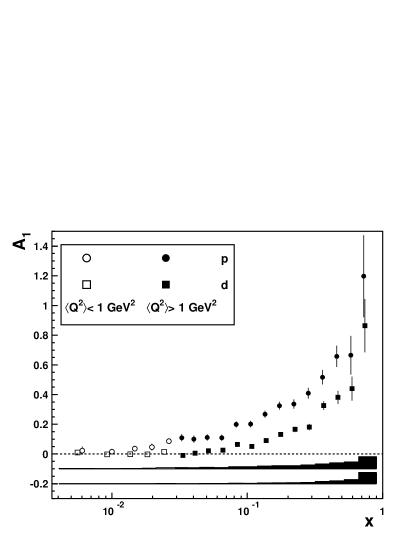
Figure 9: HERMES results on $A_{1}$ vs $x$ for proton and deuteron. Error bars represent statistical uncertainties of the data (diagonal elements of the covariance matrix) combined quadratically with those from Monte Carlo statistics. Bands represent systematic uncertainties. Deuteron data points have been slightly shifted in $x$ for visual purposes.

Figure 10: HERMES results on $A_{1}^{\textrm{p}}$and $A_{1}^{\textrm{d}}$ vs $x$, shown on separate panels, compared to data from SMC Adeva et al. (1998b, 1999, 2000), E143 Abe et al. (1998), E155 Anthony et al. (2000a), and COMPASS Ageev et al. (2005). Error bars represent the sum in quadrature of statistical and systematic uncertainties. For the HERMES data the closed (open) symbols represent values derived by selecting events with $Q^{2}>1$ GeV² ($Q^{2}<1$ GeV²). The HERMES data points shown are statistically correlated (cf. Fig. 8) by unfolding QED radiative and detector smearing effects; the statistical uncertainties shown are obtained from the diagonal elements of the covariance matrix, only. The E143 and E155 data points are correlated through QED radiative corrections. The lower panel shows the $x$ dependence of $\langle Q^{2}\rangle$ for the different experiments.

C Structure functions $g_{1}$

Proton and Deuteron.

The primary values for the structure functions $g_{1}$ for both the proton and deuteron are given in Tab. 14 for all of the 45 bins shown in Fig. 4. The correlation matrices are given in Tab. 15 for the proton and in Tab. 16 for the deuteron. For those $x$ bins having more than one $Q^{2}$ bin, the $g_{1}$ values were evolved to a common value of $Q^{2}$, as described in sect. A, and averaged. The results are shown in 19 $x$-bins in Fig. 11, together with all previously published data. Alternatively, the functions $xg_{1}^{p}$ and $xg_{1}^{d}$ are shown in Fig. 12, and compared to the previously published data in Fig. 13.

The numerical values for $g_{1}^{p,d}$ are given in Tab. 18 and the correlation matrices are in Tab. 19 for the proton and in Tab. 20 for the deuteron. When events are selected subject to $Q^{2}>1$ GeV², only 15 $x$-bins remain (see e.g. Fig. 4). The corresponding structure functions and correlation matrices are given in Tabs. 21, 23, and 24.

Figure 11: HERMES results on $g_{1}^{p}$ and $g_{1}^{d}$ vs $x$, shown on separate panels, compared to data from SMC Adeva et al. (1998b, 1999, 2000), E143 Abe et al. (1998), E155 Anthony et al. (2000a, 1999a), and COMPASS Ageev et al. (2005), in the HERMES $x$-range. Error bars represent the sum in quadrature of statistical and systematic uncertainties. The HERMES data points shown are statistically correlated (cf. Fig. 8) by unfolding QED radiative and detector smearing effects; the statistical uncertainties shown are obtained from only the diagonal elements of the covariance matrix. The E143 and E155 data points are correlated through QED radiative corrections. The E155 points have been averaged over their $Q^{2}$ bins for visibility. For the HERMES data the closed (open) symbols represent values derived by selecting events with $Q^{2}>1$ GeV² ($Q^{2}<1$ GeV²).

In the case of the proton, the central values of the SMC data points are larger than those of HERMES, in the low-$x$ region. This reflects the difference in $\langle Q^{2}\rangle$ values between the two experiments, and is expected from the $Q^{2}$ evolution of $g_{1}$.

In the case of the deuteron, the HERMES data are compatible with zero for $x<0.04$. In this region the SMC data favor negative values for $g_{1}^{d}$ while the COMPASS results Ageev et al. (2005) are also consistent with zero.

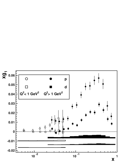
Figure 12: HERMES results for $xg_{1}$ vs $x$ for the proton and the deuteron. Error bars represent statistical uncertainties of the data (from the diagonal elements of the covariance matrix) combined quadratically with those from Monte Carlo statistics. The upper and lower error bands represent the total systematic uncertainties for the proton and deuteron, respectively. The deuteron data points have been slightly shifted in $x$ for visibility. The closed (open) symbols represent values derived by selecting events with $Q^{2}>1$ GeV² ($Q^{2}<1$ GeV²).

Figure 13: HERMES results on $xg_{1}^{p}$ and $xg_{1}^{d}$ vs $x$, shown on separate panels, compared to data from SMC Adeva et al. (1998b, 1999, 2000), E143 Abe et al. (1998), E155 Anthony et al. (2000a, 1999a), and COMPASS Ageev et al. (2005). The error bars represent the sum in quadrature of statistical and systematic uncertainties. The HERMES data points shown are statistically correlated (cf. Fig. 8) by unfolding QED radiative and detector smearing effects; the statistical uncertainties shown are obtained from only the diagonal elements of the covariance matrix. The E143 and E155 data points are correlated due to the method for correcting for QED radiation. For the HERMES data the closed (open) symbols represent values derived by selecting events with $Q^{2}>1$ GeV² ($Q^{2}<1$ GeV² ).

Neutron.

The neutron structure function $g_{1}^{n}$ is extracted from $g_{1}^{p}$ and $g_{1}^{d}$ using Eq. (23). Other nuclear effects like shadowing and Fermi motion of the nucleons in the deuteron are neglected.

Figure 14: Top panel: the structure function $g_{1}^{n}$ obtained from $g_{1}^{p}$ and $g_{1}^{d}$, compared with similar data from SMC Adeva et al. (1998b, 1999, 2000), E143 Abe et al. (1998), and E155 Anthony et al. (2000a, 1999a) in the HERMES x-range. Second panel from the top: $g_{1}^{n}$ as obtained from a ³He target by JLab Zheng et al. (2004), HERMES Ackerstaff et al. (1997), E142 Anthony et al. (1996), and E154 Abe et al. (1997b). Total error bars are shown, obtained by combining statistical and systematic uncertainties in quadrature. The bottom panel shows the $\langle Q^{2}\rangle$ of each data point in the top two panels. E155 data have been averaged over their $Q^{2}$ bins for visibility. For the HERMES data the closed (open) symbols represent values derived by selecting events with $Q^{2}>1$ GeV² ($Q^{2}<1$ GeV²).

In Fig. 14 (top panel), results on $g_{1}^{n}(x)$, extracted from $g_{1}^{p}$ and $g_{1}^{d}$, are shown for HERMES in comparison to the world data. As can be seen from the lower panel of the figure, the average $Q^{2}$ values of HERMES and SLAC measurements are similar, while those of SMC are higher by one order of magnitude at a given $x$. Compared to previous data, the HERMES measurement restricts $g_{1}^{n}(x)$ now very well. The structure function $g_{1}^{n}$ is negative everywhere, except for the very high $x$ region, where it becomes slightly positive. For decreasing $x$ values below about $0.03$, $g_{1}^{n}$ appears to gradually approach zero from below, complementary to the behavior of $g_{1}^{p}$. While this behaviour is based on data with $Q^{2}\leq 1$ GeV², it differs from the strong decrease of $g_{1}^{n}(x)$ for $x\rightarrow 0$ that was previously conjectured on the basis of the E154 measurement on ³He Abe et al. (1997b), and also on SMC data Adeva et al. (1998b), both with $Q^{2}\geq 1$ GeV² as shown in Fig. 14.

For completeness, the HERMES results on the $x$ dependence of $xg_{1}^{n}$ are shown in Fig. 15 (top panel), compared to the world data. Tabs. 25, 26 and 27 show the results for $g_{1}^{n}$ in 45 bins, 19 $x$-bins (obtained after averaging over $Q^{2}$), and in 15 $x$-bins (obtained after applying a $Q^{2}>1$ GeV² cut to data and then averaging in $Q^{2}$).

Non-singlet.

Figure 15: Top panel: $xg_{1}^{n}$ from data for $g_{1}^{p}$ and $g_{1}^{d}$. Bottom panel: the $x$-weighted non-singlet spin structure function $xg_{1}^{NS}$, compared to data from SMC Adeva et al. (1998b, 1999, 2000), E143 Abe et al. (1998), and E155 Anthony et al. (2000a, 1999a). All data are presented at their measured values of $\langle Q^{2}\rangle$, except that the E155 data in each $x$ bin have been averaged over $Q^{2}$ for visual purposes. Total uncertainties are shown as bars. For the HERMES data the closed (open) symbols represent values derived by selecting events with $Q^{2}>1$ GeV² ($Q^{2}<1$ GeV²).

The non-singlet spin structure function $g_{1}^{NS}(x,Q^{2})$ is defined as:

$$g_{1}^{NS}\equiv g_{1}^{p}-g_{1}^{n}=2\left[g_{1}^{p}-\frac{g_{1}^{d}}{1-\frac{3}{2}\omega_{D}}\right]\,.$$ (42)

In Fig. 15 (bottom panel), the $x$ dependence of $xg_{1}^{NS}$ as measured by HERMES is shown in comparison with data from E143, E155 and SMC. The non-singlet structure function shows a behavior similar to that of the deuteron and neutron, which was discussed above: the HERMES data constrain the $x$ dependence of $xg_{1}^{NS}$ much better than earlier measurements; the above-mentioned difference between the HERMES and SMC deuteron data for $x<0.03$ is reflected also in $g_{1}^{NS}$.

D Integrals of $g_{1}$

Important information about the spin structure of the nucleon can be obtained from the first moment of $g_{1}$, in particular when combining results on proton, deuteron and neutron. Experimentally, only a limited range in $x$ is accessible. The integrals for proton and deuteron over a certain $x$ range and at a given $Q^{2}_{0}$ are obtained as:

$${\widetilde{\Gamma}_{1}}(Q^{2}_{0})=\sum_{i}\frac{g_{1}(\langle x\rangle_{i},Q^{2}_{0})}{g_{1}^{fit}(\langle x\rangle_{i},Q^{2}_{0})}\int_{x_{i}}^{x_{i+1}}\!\!\!\!{\rm\,d}x\,g_{1}^{fit}(x,Q^{2}_{0}),$$ (43)

where $\langle x\rangle_{i}$ are the average values of $x$ in $x$-bin $i$ with boundaries $x_{i}$ and $x_{i+1}$; the integral of $g_{1}^{fit}$ accounts for the non-linear $x$-dependence of $g_{1}$. The integrals for $g_{1}^{n}$ and $g_{1}^{NS}$ are obtained by linearly combining the ones for proton and deuteron.

The statistical uncertainty is calculated as:

$$\sigma^{2}_{{\widetilde{\Gamma}_{1}}} = \sum_{ij}\int_{x_{i}}^{x_{i+1}}\!\!\!\!{\rm\,d}x\,g_{1}^{fit}(x,Q^{2}_{0})\int_{x_{j}}^{x_{j+1}}\!\!\!\!{\rm\,d}x\,g_{1}^{fit}(x,Q^{2}_{0})$$ (44)

$$\times\frac{\textrm{cov}\left({g_{1}}\right)_{ij}}{g_{1}^{fit}(\langle x\rangle_{i},Q^{2}_{0})~{}g_{1}^{fit}(\langle x\rangle_{j},Q^{2}_{0})}.$$

The systematic uncertainties for the integrals are determined analogously to the above described case of structure functions. The correlations between systematic uncertainties of $g_{1}^{p}$ and $g_{1}^{d}$ were taken into account in the calculation of the systematic uncertainty for $g_{1}^{n}$ and $g_{1}^{NS}$.

The integrals for $g_{1}^{p}$, $g_{1}^{d}$, $g_{1}^{n}$, and $g_{1}^{NS}$, calculated at $Q_{0}^{2}=2.5$ and $5$ GeV², are given in Tab. 6 together with the statistical, systematic and evolution uncertainties. They are shown for the $x$ range $0.021\leq x\leq 0.9$, corresponding to the event selection $Q^{2}\geq 1$ GeV². (For $x>0.0568$ the integrals over the regions $A$, $B$ and $C$ in Fig. 4 were calculated separately, found to be consistent, and then averaged.) The precision of the integrals given in Tab. 6 is less affected by the unfolding procedure since all inter-bin correlations from the unfolding procedure are taken into account. The statistical uncertainty is smaller by about 25$\%$ compared to the case when only diagonal elements of the covariance matrices are considered. Note that the error bars displayed in Figs. 11 to 15 are derived only from the diagonal elements of the covariance matrix, and the data points are statistically correlated. The individual contributions to the systematic uncertainties are displayed in Tab. 7. The systematic uncertainty is dominated by the uncertainty on the polarization measurements.

Table 6: Integrals of $g_{1}^{p}$, $g_{1}^{d}$, $g_{1}^{n}$, and $g_{1}^{NS}$. The uncertainties are separated into statistical, systematic components coming from the experiment (misalignment, particle identification and polarizations) and from the parameterizations ($R$, $F_{2}$, $A_{2}$, $A_{zz}^{d}$, $\omega_{D}$), and evolution uncertainty.

	$\displaystyle\int_{0.021}^{0.9}\!\!\!\!{\rm\,d}x\,g_{1}$	uncertainties
		stat.	syst.	par.	evol.
$Q^{2}$=2.5 GeV2
p	0.1201	0.0025	0.0068	0.0028	0.0046
d	0.0428	0.0011	0.0018	0.0008	0.0027
n	-0.0276	0.0035	0.0079	0.0031	0.0017
NS	0.1477	0.0055	0.0142	0.0055	0.0039
$Q^{2}$=5 GeV2
p	0.1211	0.0025	0.0068	0.0028	0.0050
d	0.0436	0.0012	0.0018	0.0008	0.0026
n	-0.0268	0.0035	0.0079	0.0031	0.0018
NS	0.1479	0.0055	0.0142	0.0055	0.0049

Table 7: Contributions to the total systematic uncertainty of the integrals listed in Tab. 6, over the measured $x$ range $0.021<x<0.9$, calculated at $Q^{2}_{0}=5$ GeV². The horizontal line separates the sources (experiment and parameterizations).

source	p	d	n	NS
Polarizations	0.0066	0.0017	0.0076	0.0137
$PID_{cut}$	0.0002	0.0000	0.0002	0.0003
Misalignment	0.0016	0.0006	0.0020	0.0034
$A_{2}$	0.0002	0.0001	0.0003	0.0005
$\sigma_{UU}$	0.0028	0.0008	0.0027	0.0053
$A_{zz}^{d}$	-	0.0001	0.0002	0.0002
$\omega_{D}$	-	-	0.0015	0.0015

A comparison of the integrals over the common measured $x$ range shows agreement with E143, as seen in Tab. 8. Comparisons with E155, SMC and E142 also show good agreement within uncertainties. SMC and E143 used the hypothesis that $g_{1}/F_{1}$ is independent of $Q^{2}$ to perform the evolution to a common $Q^{2}$, while E142 used the hypothesis of $Q^{2}$-independence of $A_{1}$ and E155 used QCD fits. HERMES and E143 have almost identical $\langle Q^{2}\rangle$ values at the same $x$.

Table 8: Comparisons of $g_{1}$ integrals over different measured $x$ ranges from this experiment (including the SIDIS measurement Airapetian et al. (2005a) and the measurement of $g_{1}^{n}$ from a ³He target Ackerstaff et al. (1997)) and SMC Adeva et al. (1998b), EMC Ashman et al. (1989), E143 Abe et al. (1998), E155 Anthony et al. (1999a), E142 Anthony et al. (1996), and E154 Abe et al. (1997b). In the case of E143, the normalization uncertainties, not included in the original result, have been added in quadrature to the systematic uncertainties. The results from SMC, originally in the $x$ range $0.003\leq x\leq 0.7$, as well as the results from E154, originally in the $x$ range $0.014\leq x\leq 0.7$, the results from EMC, originally in the $x$ range $0.01\leq x\leq 0.7$, and those of E155, originally in the range $0.01\leq x\leq 0.9$, have all been recalculated in the HERMES range $0.021\leq x\leq 0.7$ from the $g_{1}$ values, following the procedure used in this paper for the calculation of the HERMES moments (see Eq. (43)) and are indicated with an asterisk. In the case of EMC it was not possible to calculate uncertainties from the evolution, as the $g_{1}$ values were already at $Q^{2}=10.7$ GeV², and no evolution uncertainty was given.

Exp.	$Q^{2}_{0}$	$x$ range	type	Integral
	(GeV2)			value	stat.	syst.	param.	evol.
E143	5	0.03 - 0.8	p	0.117	0.003	0.007		-
HERMES				0.115	0.002	0.006	0.003	0.004
SMC (*)	10	0.021-0.7	p	0.120	0.005	0.007		0.002
HERMES				0.119	0.003	0.007	0.003	0.005
EMC (*)	10.7	0.021-0.7	p	0.110	0.011	0.019		-
HERMES				0.119	0.003	0.007	0.003	0.005
E155 (*)	5	0.021-0.9	p	0.124	0.002	0.009		0.005
HERMES				0.121	0.002	0.007	0.003	0.005
E143	5	0.03 - 0.8	d	0.043	0.003	0.003		-
HERMES				0.042	0.001	0.002	0.001	0.002
SMC (*)	10	0.021-0.7	d	0.042	0.005	0.004		0.001
HERMES				0.043	0.001	0.002	0.001	0.002
E155 (*)	5	0.021-0.9	d	0.043	0.002	0.003		0.003
HERMES				0.044	0.001	0.002	0.001	0.003
E142	2	0.03-0.6	n (3He)	-0.028	0.006	0.006		-
HERMES			n (p,d)	-0.025	0.003	0.007	0.002	0.001
E154 (*)	2	0.021-0.7	n (3He)	-0.032	0.003	0.005		0.003
HERMES			n (p,d)	-0.027	0.004	0.008	0.003	0.002
HERMES	2.5	0.023-0.6	n (3He)	-0.034	0.013	0.005		-
HERMES			n (p,d)	-0.027	0.003	0.007	0.003	0.001
HERMES/	2.5	0.023-0.6	NS	0.147	0.008	0.019		-
SIDIS
HERMES				0.138	0.005	0.013	0.005	0.003

For $x\rightarrow 1$, $g_{1}$ almost vanishes and a possible remaining small contribution from the region $0.9\leq x\leq 1$ to the full integral was estimated for $Q^{2}=5$ GeV² to be $0.0003\pm 0.0003$ for the proton and $0.00006\pm 0.00005$ for the deuteron, assuming a functional dependence of $g_{1}$ of the form $(1-x)^{\alpha}(1+\beta x)$ in the high-$x$ region, and fitting HERMES data alone. From these values the high-$x$ contributions to the neutron and non-singlet integrals were estimated to be $-0.0002\pm 0.0003$ and $0.0005\pm 0.0006$, respectively.

Figure 16 shows the cumulative integral of $g_{1}^{p,d,n,NS}$ as a function of the lower integration limit in $x$.

Figure 16: Integrals of $g_{1}^{p,d,n,NS}$ over the range $0.021\leq x\leq 0.9$ as a function of the low-$x$ limit of integration, evaluated at $Q^{2}=5$ GeV². Inner error bars represent total uncertainties excluding the normalization systematic uncertainty from beam and target; outer error bars include the contribution coming from the $Q^{2}$ evolution. Three of the four sets of points are slightly shifted in $x$ for visibility.

For $x<0.04$, $g_{1}^{d}(x)$ becomes compatible with zero (see also Fig. 13) and its measured integral shows saturation, while the other integrals still show the tendency of a small rise in magnitude towards lower $x$. Also, the partial first moment of $g_{1}^{d}(x)$ calculated over the range $0<x<0.021$ at $Q^{2}=5$ GeV² from the NLO QCD fit of all available data, used here for ‘evolution’, was found to be consistent with zero within one statistical standard deviation. Hence, in the remaining discussion it will be assumed that the deuteron first moment $g_{1}^{d}$ saturates for $x<0.04$. Under this assumption, conclusions can be drawn on the values of the singlet axial charge $a_{0}$ and the first moment of the singlet quark helicity distribution $\Delta\Sigma$ as well as on the strange-quark helicity distribution $\Delta s+\Delta\bar{s}$. Using the Bjorken Sum Rule, the saturation of the integral of $g_{1}^{d}$ allows an estimate of the possible contribution of the excluded region $0<x<0.021$ to the proton moment $\Gamma_{1}^{p}$.

In the following, results are given for $Q^{2}_{0}=5$ GeV² and in $\mathcal{O}(\alpha_{s}^{3})$, unless otherwise noted. The right hand side of Eq. (12) yields for the Bjorken Sum a value of $0.1821\pm 0.0004\pm 0.0019$, where the first uncertainty arises from $g_{A}/g_{V}$ and the second one from varying $\alpha_{s}$ within its limits given by the value at the $Z^{0}$ mass: $\alpha_{s}(Z^{0})=0.1187\pm 0.002$ Eidelman et al. (2004). An unambiguous test of the Bjorken Sum Rule requires the measurement of both the proton and the deuteron (neutron) integrals over the whole $x$-range. However, the proton integral does not yet saturate in the measured region, as discussed above, and therefore some uncertainty remains due to the required extrapolation into the unmeasured small-$x$ region.

The HERMES integral for the non-singlet distribution (Eq. 42) in the range $0.021<x<1$ has a value of $0.1484\pm 0.0055\mathrm{(stat.)}\pm 0.0142\mathrm{(exp.)}\pm 0.0055\mathrm{(param.)}\pm 0.0049$(evol.). This partial moment is significantly smaller than the value for the Bjorken Sum, given for various orders in Table 9, presumably because of the contribution to the proton integral from the unmeasured region at small $x$. Assuming the validity of the Bjorken Sum Rule and ignoring possible higher-twist terms Narison et al. (1995), the contribution from the unmeasured region $0<x<0.021$ to $\Gamma_{1}^{p}$ has been evaluated as the difference between the inferred value $\Gamma_{1}^{p}$(inferred) and the measured value $\widetilde{\Gamma}^{p}_{1}$ in LO to NNNLO. Its central value ranges from 0.0316 in LO to 0.0169 in NNNLO (see Table 9). The NLO value is in good agreement with earlier estimates based on QCD fits Ball et al. (1995).

By combining Eqs. (7) and (12) (with $\Delta C_{NS}=1$), this non-singlet integral can be directly compared in LO to the recently published value for $(\Delta u+\Delta\bar{u})-(\Delta d+\Delta\bar{d})$ obtained from semi-inclusive HERMES data Airapetian et al. (2005a) (see Table 8). The partial non-singlet moment is calculated at $Q^{2}_{0}=2.5$ GeV², for the sub-sample of the present data in the same kinematic range as the semi-inclusive analysis, i.e. $0.023<x<0.6$ and $Q^{2}>1$ GeV². The resulting value $6~{}\widetilde{\Gamma}_{1}^{NS}=0.828\pm 0.030\mathrm{(stat.)}\pm 0.078\mathrm{(syst.)}\pm 0.030\mathrm{(param.)}\pm 0.018$(evol.) is in agreement with the published value $(\Delta u+\Delta\bar{u})-(\Delta d+\Delta\bar{d})=0.880\pm 0.045\mathrm{(stat.)}\pm 0.107$(syst.) within the statistical uncertainties. (The experimental systematic uncertainties are highly correlated).

For convenience in the following, the argument $\alpha_{s}(Q^{2})$ of the moments of the coefficient functions will be suppressed. The deuteron first moment is given by:

$$\!\Gamma_{1}^{d}(Q^{2}_{0})\!=\!\left(1-\frac{3}{2}\omega_{D}\right)\frac{1}{36}\left[a_{8}\Delta C_{NS}^{\overline{MS}}+4a_{0}\Delta C_{S}^{\overline{MS}}\right],$$ (45)

and one obtains:

$$a_{0}(Q_{0}^{2})=\frac{1}{\Delta C_{S}^{\overline{MS}}}\left[\frac{9\Gamma_{1}^{d}}{\left(1-\frac{3}{2}\omega_{D}\right)}-\frac{1}{4}a_{8}\Delta C_{NS}^{\overline{MS}}\right].$$ (46)

Note that the Bjorken Sum Rule is not employed here. With $\alpha_{s}=0.29\pm 0.01$ for $Q^{2}_{0}=5$ GeV², and the values for $\Delta C_{NS}^{\overline{MS}}$ and $\Delta C_{S}^{\overline{MS}}$ to $\mathcal{O}(\alpha_{s}^{2})$, together with the values for $\widetilde{\Gamma}_{1}^{d}$ and $a_{8}$, the singlet axial charge yields a value $a_{0}=0.330\pm 0.011\mathrm{(theo.)}\pm 0.025\mathrm{(exp.)}\pm 0.028$(evol.).

Table 9: Expected Bjorken Sum (BJS) calculated in LO through NNNLO, at $Q^{2}=5$ GeV², with uncertainties coming from $g_{A}/g_{V}$ and $\alpha_{s}$. For the proton, the inferred value of $\Gamma_{1}^{p}$ in the table is obtained using the BJS and the measured $\Gamma_{1}^{d}$ (assuming $\Gamma_{1}^{d}=\widetilde{\Gamma}^{d}_{1}$); its first uncertainty comes from $g_{A}/g_{V}$, $\alpha_{s}$, and $\omega_{D}$, the second from $\Gamma_{1}^{d}$ (statistical and systematic), while the last one comes from the $Q^{2}$ evolution. Using the measured value for $\widetilde{\Gamma}_{1}^{p}$ and assuming the validity of the Bjorken Sum Rule, the missing part of the proton integral due to the low-$x$ region is estimated in the last column; its first uncertainty comes from $g_{A}/g_{V}$, $\alpha_{s}$ and $\omega_{D}$, the second from $\Gamma_{1}^{p}$ (statistical and systematic), the third from $\Gamma_{1}^{d}$ (statistical and systematic), while the last one comes from the $Q^{2}$ evolution on both $\Gamma_{1}^{p}$ and $\Gamma_{1}^{d}$.

		BJS	$\Gamma_{1}^{p}$(inferred)	Estimated $\Gamma_{1}^{p}-\widetilde{\Gamma}^{p}_{1}$
LO	${\cal O}(\alpha_{s}^{0})$	$0.2116\pm 0.0005$	$0.1530\pm 0.0008\pm 0.0025\pm 0.0028$	$0.0316\pm 0.0008\pm 0.0025\pm 0.0079\pm 0.0025$
NLO	${\cal O}(\alpha_{s}^{1})$	$0.1923\pm 0.0009$	$0.1434\pm 0.0008\pm 0.0025\pm 0.0028$	$0.0219\pm 0.0008\pm 0.0025\pm 0.0079\pm 0.0025$
NNLO	${\cal O}(\alpha_{s}^{2})$	$0.1856\pm 0.0015$	$0.1400\pm 0.0009\pm 0.0025\pm 0.0028$	$0.0186\pm 0.0009\pm 0.0025\pm 0.0079\pm 0.0025$
NNNLO	${\cal O}(\alpha_{s}^{3})$	$0.1821\pm 0.0019$	$0.1383\pm 0.0013\pm 0.0025\pm 0.0028$	$0.0169\pm 0.0013\pm 0.0025\pm 0.0079\pm 0.0025$

It is interesting to note that the deuteron target has an intrinsic advantage over the proton target with respect to the precision that can be achieved in the determination of $a_{0}$ from $\Gamma_{1}$, in the typical case that the uncertainty in $\Gamma_{1}$ is dominated by scale uncertainties associated with beam and target polarization. This is because the magnitude of $\Gamma_{1}^{d}$ is only about 30% of that of $\Gamma_{1}^{p}$, so that a similar scale uncertainty produces a correspondingly smaller absolute uncertainty in $\Gamma_{1}^{d}$, and as a consequence also in $a_{0}$. This advantage of deuterium can be expected to be also reflected in the impact of such data on the precision of global QCD fits.

The interpretation of quark distributions and their moments extracted in NLO is subject to some ambiguity due to their scheme dependence. Nevertheless some conclusions can be drawn, especially for the sake of comparison to earlier results, if one stays within the $\overline{MS}$ scheme. In this scheme $a_{0}$ can be identified with $\Delta\Sigma$: $a_{0}\stackrel{{\scriptstyle\scriptstyle\overline{MS}}}{{=}}\Delta\Sigma=(\Delta u+\Delta\bar{u})+(\Delta d+\Delta\bar{d})+(\Delta s+\Delta\bar{s})$. The value obtained for $\Delta\Sigma(Q_{0}^{2}=5$ GeV${}^{2})$ is compared with other results from both experimental analyses and QCD fits in Tab. 28. The HERMES value obtained from $\widetilde{\Gamma}_{1}^{d}$ is in good agreement with the earlier E143 result Abe et al. (1998) on the same target at $Q^{2}=3$ GeV², but less so with the SMC result Adeva et al. (1998b) at $Q^{2}=10$ GeV². The HERMES value represents about 55$\%$ of the relativistic QPM expectation of 0.6. The HERMES data therefore suggest that the quark helicities contribute a substantial fraction to the nucleon helicity, but there is still need for a considerable contribution from gluons and/or orbital angular momenta.

From Tab. 28 it can be seen that, among results for $\Delta\Sigma$ extracted from the data of individual experiments, those using estimates of the contribution from small $x$ based on NLO QCD fits tend to give systematically smaller values that are more consistent with the QCD-fit values of $\Delta\Sigma$ in the lower section of the table. This emphasizes the importance of the unmeasured region at small $x$. We note that the partial first moment of $\Delta\Sigma(x)$ calculated over the range $0<x<0.021$ at $Q^{2}=5$ GeV² from the NLO QCD fit of all available data that is used here for ‘evolution’ is found to be $-0.1334\pm 0.1104\mathrm{(stat.)}\pm 0.0273\mathrm{(syst.)}\pm 0.0604$(theo.). It may also be relevant that all of the NLO QCD fits listed here differ from the direct extractions in that they impose symmetry among the sea flavours, and invoke the Bjorken Sum Rule.

Under the assumption of SU(3) symmetry, the first moment of the strange-quark helicity distribution can be obtained from the relation

$$\Delta s+\Delta\bar{s}=\frac{1}{3}\left(a_{0}-a_{8}\right)\\ =\frac{1}{\Delta C_{S}^{\overline{MS}}}\!\left[\frac{3\Gamma_{1}^{d}}{(1-\frac{3}{2}\omega_{d})}-\frac{a_{8}\left(4\Delta C_{S}^{\overline{MS}}+\Delta C_{NS}^{\overline{MS}}\right)}{12}\right]\,.$$ (47)

The value $\Delta s+\Delta\bar{s}=-0.085\pm 0.013\mathrm{(theo.)}\pm 0.008\mathrm{(exp.)}\pm 0.009$(evol.) is obtained from HERMES deuteron data, in order ${\cal{O}}(\alpha_{s}^{2})$. This value is negative and different from zero by about 4.7 $\sigma$.

The above results are based on the assumption of the validity of SU(3) flavor symmetry in hyperon $\beta$-decays. The validity of this assumption is open to question. A recent analysis  Ratcliffe (2004) of such data leads, however, to the conclusion that such symmetry breaking effects are small. Even if we assume that SU(3) symmetry is broken by up to 20$\%$ and that $a_{8}$ lies in the range $0.47\leq a_{8}\leq 0.70$, the above conclusions are little changed and one obtains $0.358\geq a_{0}\geq 0.302$ and $-0.037\leq\Delta s+\Delta\bar{s}\leq-0.133$. It is interesting to note that a recent global NLO fit of the previous world data for polarized inclusive and semi-inclusive deep-inelastic scattering De Florian et al. (2005), which was made without the assumption of SU(3) flavor symmetry, results in a small SU(3) breaking of -1% to -8%, a value of $\Delta s$ between -0.045 and -0.051 and a value of $\Delta\Sigma$ between 0.284 and 0.311, depending on the set of NLO fragmentation functions used in the analysis.

Values for $\Delta u+\Delta\bar{u}$ and $\Delta d+\Delta\bar{d}$ can be determined in the $\overline{MS}$ scheme using as experimental input the value of $a_{0}$ extracted from the deuteron data and as additional input the values for the matrix elements $a_{3}$ and $a_{8}$:

$$\Delta u+\Delta\bar{u} = \frac{1}{6}[2a_{0}+a_{8}+3a_{3}]\,,$$

$$\Delta d+\Delta\bar{d} = \frac{1}{6}[2a_{0}+a_{8}-3a_{3}].$$ (48)

The values $\Delta u+\Delta\bar{u}=0.842\pm 0.004\mathrm{(theo.)}\pm 0.008\mathrm{(exp.)}\pm 0.009$(evol.) and $\Delta d+\Delta\bar{d}=-0.427\pm 0.004\mathrm{(theo.)}\pm 0.008\mathrm{(exp.)}\pm 0.009$(evol.) are obtained. These results are essentially free from uncertainties due to extrapolations of $g_{1}$ towards $x=0$, provided the integral for $g_{1}^{d}$ really saturates at $x<0.04$, but they invoke the validity of the Bjorken Sum Rule.

The values for $a_{0}$, $\Delta u+\Delta\bar{u}$, $\Delta d+\Delta\bar{d}$, and $\Delta s+\Delta\bar{s}$ have been calculated in LO, NLO and NNLO from the deuteron integral and are shown in Table 10.

Table 10: Values for $a_{0}$, $\Delta u+\Delta\bar{u}$, $\Delta d+\Delta\bar{d}$, and $\Delta s+\Delta\bar{s}$ calculated according to Eqs. (46), (47), and (D) at $Q^{2}=5$ GeV². Uncertainties are separated into theoretical ($a_{3}$, $a_{8}$ and $\alpha_{s}$) and those coming from the uncertainty of $\widetilde{\Gamma}_{1}^{d}$ (where ’exp.’ includes statistical, systematic, and parameterizations, while ’evol.’ comes from the evolution).

		central	uncertainties
		value	theor.	exp.	evol.
$a_{0}$
LO	${\cal O}(\alpha_{s}^{0})$	0.278	0.010	0.022	0.025
NLO	${\cal O}(\alpha_{s}^{1})$	0.321	0.011	0.024	0.028
NNLO	${\cal O}(\alpha_{s}^{2})$	0.330	0.011	0.025	0.028
$\Delta u+\Delta\bar{u}$
LO	${\cal O}(\alpha_{s}^{0})$	0.825	0.004	0.007	0.008
NLO	${\cal O}(\alpha_{s}^{1})$	0.839	0.004	0.008	0.009
NNLO	${\cal O}(\alpha_{s}^{2})$	0.842	0.004	0.008	0.009
$\Delta d+\Delta\bar{d}$
LO	${\cal O}(\alpha_{s}^{0})$	-0.444	0.004	0.007	0.008
NLO	${\cal O}(\alpha_{s}^{1})$	-0.430	0.004	0.008	0.009
NNLO	${\cal O}(\alpha_{s}^{2})$	-0.427	0.004	0.008	0.009
$\Delta s+\Delta\bar{s}$
LO	${\cal O}(\alpha_{s}^{0})$	-0.103	0.013	0.007	0.008
NLO	${\cal O}(\alpha_{s}^{1})$	-0.088	0.013	0.008	0.009
NNLO	${\cal O}(\alpha_{s}^{2})$	-0.085	0.013	0.008	0.009

They are somewhat different from the partial moments that were previously extracted in LO by HERMES from semi-inclusive DIS data: $\int_{0.023}^{0.6}(\Delta u+\Delta\bar{u})\,\mathrm{d}x=0.599\pm 0.022\pm 0.065$, $\int_{0.023}^{0.6}(\Delta d+\Delta\bar{d})\,\mathrm{d}x=-0.280\pm 0.026\pm 0.057$, and $\int_{0.023}^{0.3}\Delta s\,\mathrm{d}x=0.028\pm 0.033\pm 0.009$ Airapetian et al. (2005a). These partial moments for the up- and down-quark helicity distributions are smaller in magnitude than the full moments given in Table 9, due to the restricted $x$-range. They also do not invoke the validity of the Bjorken Sum Rule. One possible explanation of the difference between the above quoted partial moment of the strange-quark helicity distribution and the value for $\frac{1}{2}(\Delta s+\Delta\bar{s})$ derived in this analysis could be a substantial negative contribution to it at small $x$.

VII Conclusions

HERMES has measured the spin structure function $g_{1}(x,Q^{2})$ of the proton and the deuteron in the kinematic range $0.0041<x<0.90$ and $0.18$ GeV²$<Q^{2}<20$ GeV². By combining the proton and the deuteron data, the neutron spin structure function $g_{1}^{n}(x,Q^{2})$ is extracted.

In the HERMES analysis, the measured asymmetries are corrected for detector smearing and QED radiative effects by applying an unfolding algorithm. As a consequence, the resulting data points are no longer correlated systematically but instead statistically. The full information on the statistical correlations is contained in the covariance matrix. In order to avoid overestimating the statistical uncertainties, it is mandatory to take into account its off-diagonal elements when using the HERMES data for any further analysis. A fair comparison of the statistical power of different experiments is given by the accuracy of integrals of structure functions.

The statistical precision of the HERMES proton data is comparable to that of the hitherto most precise data from SLAC and CERN in the same $x$ range. The HERMES deuteron data provide the most precise published determination of the spin structure function $g_{1}^{d}(x,Q^{2})$, compared to previous measurements. In the region $x<0.03$ the SMC data favor negative values, while the HERMES deuteron data are compatible with zero, as are the recent COMPASS data.

The combination of the HERMES measurements of $g_{1}^{p}$ and $g_{1}^{d}$ constrains the neutron spin structure function $g_{1}^{n}(x)$ well. Its accuracy is comparable to the E154 result that is obtained from a ${}^{3}He$ target. Its behavior in the region $x<0.03$ with $\langle Q^{2}\rangle<1$ GeV² differs from the dramatic drop-off of $g_{1}^{n}(x)$ for $x\rightarrow 0$, earlier conjectured on the basis of previous data.

Integrals of the spin structure function $g_{1}$ of proton, deuteron and neutron have been calculated in various $x$-ranges and values of $Q^{2}_{0}$. The HERMES proton integral agrees with E143 and within statistical uncertainties also with SMC, at their respective $Q^{2}_{0}$-values. The HERMES deuteron integral improves on the accuracy (statistical combined with systematic) of previous results. It appears to saturate for $x<0.04$. Assuming this saturation, the first moment of the deuteron structure function $g_{1}(x,Q^{2})$ can be determined with small uncertainties due to the extrapolation of $g_{1}^{d}$ towards $x=0$. It yields $\Gamma_{1}^{d}(Q^{2}=5$ GeV${}^{2})=0.0437\pm 0.0035$(total). The difference of twice the proton integral in the measured range, $\widetilde{\Gamma}_{1}^{p}=0.1214\pm 0.0093$(total) and the first deuteron moment, corrected for the D-wave admixture to the deuteron wave function, amounts to $\widetilde{\Gamma}_{1}^{NS}=0.1484\pm 0.0170$(total). It agrees within 2 $\sigma$ with the Bjorken Sum Rule, $\Gamma_{1}^{NS}=0.1821\pm 0.0019$, calculated in QCD in $\mathcal{O}(\alpha_{s}^{3})$. From the difference of the theoretical value and the measured value, the contribution of the excluded region $0\leq x<0.021$ to the first proton moment $\Gamma_{1}^{p}$ is estimated to yield only $0.017\pm 0.009$.

Based on the assumed saturation of the integral of $g_{1}^{d}$ and with the assumption of SU(3) flavor symmetry in the decays of hyperons in the spin-$\frac{1}{2}$ baryon octet, the flavor-singlet axial charge $a_{0}$ has been determined in the $\overline{MS}$ scheme using $\Gamma_{1}^{d}$ and the axial charge $a_{8}$ as inputs, in order $\alpha_{s}^{2}$. It amounts to

$$\bm{a_{0}}(Q^{2}=5\,\mathrm{GeV}^{2})\bm{=}\\ \bm{0.330\pm 0.011}\mathrm{(theo.)}\bm{\pm 0.025}\mathrm{(exp.)}\bm{\pm 0.028}\mathrm{(evol.).}$$ (49)

In this factorization scheme, this result can be interpreted as the contribution $\Delta{\Sigma}$ of quark helicities to the nucleon helicity. The HERMES data therefore suggest that the quark helicities contribute a substantial fraction to the nucleon helicity, but there is still need for a major contribution from gluons and/or orbital angular momenta of more than half of the sum of Eq. (1). Under the same assumptions, a negative value for the first moment of the helicity distribution for strange quarks $\Delta s+\Delta\bar{s}=-0.085\pm 0.013\mathrm{(theo.)}\pm 0.008\mathrm{(exp.)}\pm 0.009$(evol.) is obtained from the deuteron data, in order $\alpha_{s}^{2}$.

Values for $\Delta u+\Delta\bar{u}$ and $\Delta d+\Delta\bar{d}$ have been determined in the $\overline{MS}$ scheme using $\Gamma_{1}^{d}$ and the axial charges $a_{3}$ and $a_{8}$ as inputs, and the values $\Delta u+\Delta\bar{u}=0.842\pm 0.004\mathrm{(theo.)}\pm 0.008\mathrm{(exp.)}\pm 0.009$(evol.) and $\Delta d+\Delta\bar{d}=-0.427\pm 0.004\mathrm{(theo.)}\pm 0.008\mathrm{(exp.)}\pm 0.009$(evol.) are obtained.

Appendix A Unfolding algorithm

An unfolding algorithm was used to correct the asymmetries for the kinematic smearing effects of higher order QED processes and the spectrometer resolution. The complexity of such an algorithm stems from the fact that the calculable absolute cross section of the spin-dependent radiative background processes, e.g., ‘elastic tails’, must be effectively normalized to the data by comparing simulated and measured unpolarized yields based on world data on $\sigma_{UU}$.

Radiative effects include vertex corrections to the QED hard scattering amplitude, and kinematic migration due to radiation of real photons by the lepton in either the initial (ISR) or final (FSR) state. Also ISR may in principle flip the helicity of the incident lepton before it emits the virtual photon Contopanogos and Einhorn (1992), reducing the effective ‘photon depolarization parameter’ to a degree that is correlated with kinematic migration. Thus this additional ‘spin-state mixing’ doubles the size of the smearing matrix, as the kinematic bins for the two spin states are coupled. This generality is retained here for pedagogical reasons in spite of the suppression of ‘helicity-flip bremsstrahlung’ by an additional power of $\alpha$.

Our basic assumption here is that radiative effects on the observed experimental cross sections $\sigma^{X}(\bm{x})$ ($X$ signifying experimental), depending on various kinematic parameters collectively designated $\bm{x}$, can be represented by a pair of coupled integral equations containing elements of a matrix of radiative kernels ${\cal K}$:

$$\!\!\!\!\!\!\!\!\sigma^{X}_{\stackrel{{\scriptstyle\rightarrow}}{{\Leftarrow}}}(\bm{x})\!\!\! = \!\!\!\int\!\!\!{\rm\,d}\bm{t}\left[{\cal K}_{{\stackrel{{\scriptstyle\rightarrow}}{{\Leftarrow}}}{\stackrel{{\scriptstyle\rightarrow}}{{\Leftarrow}}}}(\bm{x},\bm{t})\,\sigma_{\frac{1}{2}}(\bm{t})+{\cal K}_{{\stackrel{{\scriptstyle\rightarrow}}{{\Leftarrow}}}{\stackrel{{\scriptstyle\rightarrow}}{{\Rightarrow}}}}(\bm{x},\bm{t})\,\sigma_{\frac{3}{2}}(\bm{t})\right]$$ (50)

$$\!\!\!\!\!\!\!\!\sigma^{X}_{\stackrel{{\scriptstyle\rightarrow}}{{\Rightarrow}}}(\bm{x})\!\!\! = \!\!\!\int\!\!\!{\rm\,d}\bm{t}\left[{\cal K}_{{\stackrel{{\scriptstyle\rightarrow}}{{\Rightarrow}}}{\stackrel{{\scriptstyle\rightarrow}}{{\Leftarrow}}}}(\bm{x},\bm{t})\,\sigma_{\frac{1}{2}}(\bm{t})+{\cal K}_{{\stackrel{{\scriptstyle\rightarrow}}{{\Rightarrow}}}{\stackrel{{\scriptstyle\rightarrow}}{{\Rightarrow}}}}(\bm{x},\bm{t})\,\sigma_{\frac{3}{2}}(\bm{t})\right].$$ (51)

Here the radiative (quasi-)elastic (Bethe-Heitler) background is included by continuing the integrals up to $x_{Bj}=1$. (We neglect the small contribution from the transverse asymmetry $A_{2}$.) Because parity is conserved in QED, we have

$${\cal K}_{{\stackrel{{\scriptstyle\rightarrow}}{{\Leftarrow}}}{\stackrel{{\scriptstyle\rightarrow}}{{\Leftarrow}}}} = {\cal K}_{{\stackrel{{\scriptstyle\rightarrow}}{{\Rightarrow}}}{\stackrel{{\scriptstyle\rightarrow}}{{\Rightarrow}}}}\ \equiv\ {\cal K}_{diag}$$ (52)

$${\cal K}_{{\stackrel{{\scriptstyle\rightarrow}}{{\Leftarrow}}}{\stackrel{{\scriptstyle\rightarrow}}{{\Rightarrow}}}} = {\cal K}_{{\stackrel{{\scriptstyle\rightarrow}}{{\Rightarrow}}}{\stackrel{{\scriptstyle\rightarrow}}{{\Leftarrow}}}}\ \equiv\ {\cal K}_{off}\,.$$ (53)

In the absence of radiative effects, these equations simplify to represent the Born-approximation cross section $\sigma^{B}(\bm{x})$ as:

$$\sigma^{B}_{\stackrel{{\scriptstyle\rightarrow}}{{\Leftarrow}}}(\bm{x}) = \left[{\cal K}^{B}_{diag}(\bm{x})\,\sigma_{\frac{1}{2}}(\bm{x})+{\cal K}^{B}_{off}(\bm{x})\,\sigma_{\frac{3}{2}}(\bm{x})\right]$$ (54)

$$\sigma^{B}_{\stackrel{{\scriptstyle\rightarrow}}{{\Rightarrow}}}(\bm{x}) = \left[{\cal K}^{B}_{off}(\bm{x})\,\sigma_{\frac{1}{2}}(\bm{x})+{\cal K}^{B}_{diag}(\bm{x})\,\sigma_{\frac{3}{2}}(\bm{x})\right].$$ (55)

In this case, we can recognize the coefficients as representing the effective ‘depolarization parameter’:

$$D(\bm{x})=\frac{{\cal K}^{B}_{diag}(\bm{x})-{\cal K}^{B}_{off}(\bm{x})}{{\cal K}^{B}_{diag}(\bm{x})+{\cal K}^{B}_{off}(\bm{x})}\,.$$ (56)

Figure 17: Migration matrices $M_{{\stackrel{{\scriptstyle\rightarrow}}{{\Rightarrow}}}}$ (the $M_{{\stackrel{{\scriptstyle\rightarrow}}{{\Leftarrow}}}}$ matrices look similar) for two different binnings. Left panel: migration matrix for a pure $x$ binning. Right panel: migration matrix for the combined $x$ and $Q^{2}$ binning used in this analysis. The horizontal and vertical lines divide the $x$-bins; within each $x$-bin the $Q^{2}$ bins are arranged in increasing $Q^{2}$. The matrices are extracted from a fully reconstructed Monte Carlo data set simulating both QED radiative and detector effects for inclusive DIS on a proton target.

Inverting Eqs. (54)–(55) and substituting in Eqs. (50)–(51), we obtain equations relating Born and measured yields, of the form:

$$\!\!\!\!\!\!\!\!\sigma^{X}_{\stackrel{{\scriptstyle\rightarrow}}{{\Leftarrow}}}(\bm{x})\!\!\! = \!\!\!\int\!\!\!{\rm\,d}\bm{t}\left[{\cal K}^{\prime}_{diag}(\bm{x},\bm{t})\,\sigma^{B}_{\stackrel{{\scriptstyle\rightarrow}}{{\Leftarrow}}}(\bm{t})+{\cal K}^{\prime}_{off}(\bm{x},\bm{t})\,\sigma^{B}_{\stackrel{{\scriptstyle\rightarrow}}{{\Rightarrow}}}(\bm{t})\right]$$ (57)

$$\!\!\!\!\!\!\!\!\sigma^{X}_{\stackrel{{\scriptstyle\rightarrow}}{{\Rightarrow}}}(\bm{x})\!\!\! = \!\!\!\int\!\!\!{\rm\,d}\bm{t}\left[{\cal K}^{\prime}_{off}(\bm{x},\bm{t})\,\sigma^{B}_{\stackrel{{\scriptstyle\rightarrow}}{{\Leftarrow}}}(\bm{t})+{\cal K}^{\prime}_{diag}(\bm{x},\bm{t})\,\sigma^{B}_{\stackrel{{\scriptstyle\rightarrow}}{{\Rightarrow}}}(\bm{t})\right].$$ (58)

For the analysis of experimental data, the kernels in these equations are modified to also account for the smearing effects of instrumental resolution. The resulting equations are discretized by dividing the experimental (Born) kinematic space into $n_{i}$ ($n_{j}$) bins, with $n_{i}\leq n_{j}$. It is convenient to work in the $2n_{i}$ ($2n_{j}$) dimensional space containing vectors consisting of $n_{i}$ ($n_{j}$) event yields for the ${\stackrel{{\scriptstyle\rightarrow}}{{\Leftarrow}}}$ spin state followed by the same number for the ${\stackrel{{\scriptstyle\rightarrow}}{{\Rightarrow}}}$ state. The yield vectors binned in experimental and Born variables are related via the discretization of Eqs. (57)–(58):

$$N^{X}=SN^{B}+N^{bg}\,,$$ (59)

where $N^{X}$ ($N^{B}$) is a vector of length $2n_{i}$ ($2n_{j}$) representing experimental (Born) yields, and $S$ is a $2n_{i}\times 2n_{j}$ smearing matrix. The two $n_{i}\times n_{j}$ equal off-diagonal quarters of $S$ are designated $S_{off}$, and correspond to ${\cal K}^{\prime}_{off}$ in Eqs. (57)–(58), while the diagonal quarters $S_{diag}$ correspond to ${\cal K}^{\prime}_{diag}$. As none of the kinematic bins are assumed to include the value $x_{Bj}=1$, the additional $2n_{i}$-vector $N^{bg}$ appears to account for the background contribution from the Bethe-Heitler process as well as kinematic migration into the acceptance from outside.

The smearing matrix $S$ is extracted from two Monte Carlo simulations. One simulation accounts for QED radiative effects and includes complete detector simulation, followed by standard event reconstruction. Hence kinematic smearing from both radiative and instrumental effects are included. Radiative processes and vertex corrections have been computed using the method outlined in Ref. Akushevich et al. (1998). The elastic and quasi-elastic radiative backgrounds have been evaluated using parameterizations of the nucleon form factors  Gari and Krümpelmann (1985) and the deuteron form factors  Locher and Svarc (1991). For the deuteron, the reduction of the bound nucleon cross section with respect to that for the free nucleon (quasi-elastic suppression) was evaluated using the results from Ref. Bernabeu (1972). The DIS event generator uses parameterizations representing the world data for $\sigma_{UU}$ Abramowicz and Levy (1997); Whitlow et al. (1990). The events were generated in the angular range $|\theta_{x}|<180$ mrad, $35$ mrad $<|\theta_{y}|<150$ mrad of observed kinematics. The electrons are tracked through a detailed GEANT Brun et al. (1978) model of the HERMES spectrometer and reconstructed with the same HRC Ackerstaff et al. (1998) reconstruction algorithm as for real data.

For each simulated event, the calculation provides both the kinematic values reconstructed from the spectrometer as well as the ‘Born’ values describing the primary QED vertex where the incident lepton emits the virtual photon. Hence those Monte Carlo events for spin state, e.g., ${\stackrel{{\scriptstyle\rightarrow}}{{\Leftarrow}}}$ that are selected under the same criteria that are applied to the analysis of experimental data can be sorted into a $n_{i}\times n_{j}$ ‘migration matrix’ $M_{\stackrel{{\scriptstyle\rightarrow}}{{\Leftarrow}}}$, where $M_{\stackrel{{\scriptstyle\rightarrow}}{{\Leftarrow}}}(i,j)$ contains the yield of events originating in Born bin $j$ and smeared into experimental bin $i$. Background events originating from the Bethe-Heitler process or from outside the acceptance are not included in $M$.

As an example, Fig. 17 illustrates the migration matrix $M_{{\stackrel{{\scriptstyle\rightarrow}}{{\Rightarrow}}}}(i,j)$. An $x$ distribution like the one in Fig. 6 represents a slice along a given Born bin $j$ in the matrix that is shown in the left panel of Fig. 17. In the right panel of Fig. 17, a migration matrix for the two-dimensional $x$-$Q^{2}$ binning is displayed. As the unfolding procedure is oblivious to the kinematic proximity of the bins, it can be used for any kind of kinematic binning. Therefore a two-dimensional smearing problem can simply be reduced to a one-dimensional problem.

The migration matrices are related to the smearing matrix via the vector $N^{B}$ of Born yields. The vector $N^{B}$ is not available from the same Monte Carlo simulation, as some events from inside the nominal kinematic acceptance migrate outside and are lost. Hence $N^{B}$ is obtained from a second Monte Carlo simulation with the same luminosity but with both radiative and instrumental effects omitted. We designate ${\cal N}^{B}_{\stackrel{{\scriptstyle\rightarrow}}{{\Leftarrow}}}$ and ${\cal N}^{B}_{\stackrel{{\scriptstyle\rightarrow}}{{\Rightarrow}}}$ to be the $n_{j}\times n_{j}$ diagonal matrices with diagonal elements that are respectively the first and second halves of $N^{B}$. Then the migration matrices can be written as

$$M_{\stackrel{{\scriptstyle\rightarrow}}{{\Leftarrow}}} = S_{diag}\,{\cal N}^{B}_{\stackrel{{\scriptstyle\rightarrow}}{{\Leftarrow}}}+S_{off}\,{\cal N}^{B}_{\stackrel{{\scriptstyle\rightarrow}}{{\Rightarrow}}}$$ (60)

$$M_{\stackrel{{\scriptstyle\rightarrow}}{{\Rightarrow}}} = S_{diag}\,{\cal N}^{B}_{\stackrel{{\scriptstyle\rightarrow}}{{\Rightarrow}}}+S_{off}\,{\cal N}^{B}_{\stackrel{{\scriptstyle\rightarrow}}{{\Leftarrow}}}\,.$$ (61)

If we define a discriminant ${\cal D}\equiv{\cal N}^{B}_{\stackrel{{\scriptstyle\rightarrow}}{{\Leftarrow}}}{\cal N}^{B}_{\stackrel{{\scriptstyle\rightarrow}}{{\Leftarrow}}}-{\cal N}^{B}_{\stackrel{{\scriptstyle\rightarrow}}{{\Rightarrow}}}{\cal N}^{B}_{\stackrel{{\scriptstyle\rightarrow}}{{\Rightarrow}}}$, the above equations can be solved to yield:

$$S_{diag} = \left[M_{\stackrel{{\scriptstyle\rightarrow}}{{\Leftarrow}}}\,{\cal N}^{B}_{\stackrel{{\scriptstyle\rightarrow}}{{\Leftarrow}}}-M_{\stackrel{{\scriptstyle\rightarrow}}{{\Rightarrow}}}\,{\cal N}^{B}_{\stackrel{{\scriptstyle\rightarrow}}{{\Rightarrow}}}\right]{\cal D}^{-1}$$ (62)

$$S_{off} = \left[M_{\stackrel{{\scriptstyle\rightarrow}}{{\Rightarrow}}}\,{\cal N}^{B}_{\stackrel{{\scriptstyle\rightarrow}}{{\Leftarrow}}}-M_{\stackrel{{\scriptstyle\rightarrow}}{{\Leftarrow}}}\,{\cal N}^{B}_{\stackrel{{\scriptstyle\rightarrow}}{{\Rightarrow}}}\right]{\cal D}^{-1}\,.$$ (63)

Then $S$ can be assembled from $S_{diag}$ and $S_{off}$. The off-diagonal terms give rise to some dependence on the Monte Carlo model for $N^{B}$. The smearing matrix for polarization-averaged data is given by $S_{u}=S_{diag}+S_{off}$.

The experimental yields need have no absolute normalization in order to subtract the calculable Bethe-Heitler background because the polarization-averaged cross section has been measured with high precision. Those two known cross sections are encoded in the Monte Carlo event generator. Hence effectively normalizing the polarization-averaged Monte Carlo yields to the observed yields results in properly normalized Bethe-Heitler background yields from the Monte Carlo. Representing this scheme here requires transformation of the ${\stackrel{{\scriptstyle\rightarrow}}{{\Leftarrow}}}$ and ${\stackrel{{\scriptstyle\rightarrow}}{{\Rightarrow}}}$ variables into polarization-averaged and polarization-difference variables. The $n_{i}$-vector of polarization-averaged yields $N^{X}_{u}$ can be obtained through application of an $n_{i}\times 2n_{i}$ projector matrix $U$ (signifying Unpolarized). $U$ is constructed by juxtaposing two $n_{i}\times n_{i}$ diagonal matrices, with all diagonal elements of both left and right half equal to $\frac{1}{2}$. Similarly, the vector of polarization-difference yields $N^{X}_{p}$ can be obtained by application of the projector $P$, which differs from $U$ only in that the diagonal elements of the right-hand half are $-\frac{1}{2}$. Thus we have

$$N^{X}_{u} = U(SN^{B}+N^{bg})=S_{u}N^{B}_{u}+UN^{bg}$$ (64)

$$N^{X}_{p} = P(SN^{B}+N^{bg})\,.$$ (65)

Eq. (59) applies to the results of the Monte Carlo simulation, which is assumed to describe reality with the possible exception of unsimulated polarization-independent detector inefficiencies. A similar equation relates the vectors representing the measured experimental yields $X$ and the corresponding unknown Born yields $B$, the polarization asymmetry $A_{||}$ of which is the goal of the analysis. We represent the detector efficiencies in this equation as the elements of an $n_{i}\times n_{i}$ diagonal matrix $K_{n}$. It is convenient to construct a $2n_{i}\times 2n_{i}$ diagonal matrix $K_{2n}$ by repeating $K_{n}$ as the diagonal quarters. These constructions are related by $UK_{2n}=K_{n}U$ and similarly for $P$. The smearing of the experimental data is then given by:

$$X = K_{2n}SB+X^{bg}$$ (66)

$$X_{u} = U(K_{2n}SB+X^{bg})=K_{n}S_{u}B_{u}+UX^{bg}\$$ (67)

$$X_{p} = P(K_{2n}SB+X^{bg})\,.$$ (68)

The Monte Carlo normalization relative to the experimental data is arbitrary. This is represented here in terms of an arbitrary constant $c$ relating the polarization-averaged Born yields $N^{B}_{u}$ from the Monte Carlo generator to $B$ corresponding to the experimental observations:

$$B_{u}=cN^{B}_{u}\,.$$ (69)

The Monte Carlo also correctly describes the entire polarization-dependent background $N^{bg}$ and its relationship to the polarization-averaged yields. Hence the same normalization constant applies to the background terms:

$$X^{bg}=cK_{2n}N^{bg}\,.$$ (70)

Combining this relation with Eqs. (64), (67) and (69), we have:

$$X_{u}=cK_{n}N^{X}_{u}\,.$$ (71)

Note that such a relationship does not generally hold for $X_{p}$, as the Monte Carlo model for $N^{X}_{p}$ need not describe reality.

Rearranging Eq. (64) and applying Eq. (69), we get:

$$USB=c\left[N^{X}_{u}-UN^{bg}\right]\,.$$ (72)

The diagonal $n_{i}\times n_{i}$ matrix $A^{m}_{||}$ containing the measured asymmetries is defined as

$$A^{m}_{||}(i,i)\equiv\frac{X_{p}(i)}{X_{u}(i)}\,.$$ (73)

Then applying Eq. (68), we get:

$$A^{m}_{||}X_{u}=X_{p}=P(K_{2n}SB+X^{bg})\,.$$ (74)

Rearranging, applying Eqs. (70), (71) and $PK_{2n}=K_{n}P$, and then multiplying both sides by $K_{n}^{-1}$, we get

$$PK_{2n}SB = A^{m}_{||}X_{u}-PX^{bg}$$

$$PSB = c\left[A^{m}_{||}N^{X}_{u}-PN^{bg}\right]\,,$$ (75)

where we have used $A^{m}_{||}K_{n}=K_{n}A^{m}_{||}$, as both $K_{n}$ and $A^{m}_{||}$ are diagonal. We now stack the two $n_{i}\times 2n_{i}$ projector matrices $U$ and $P$ to form the $2n_{i}\times 2n_{i}$ projector $\left\{\begin{array}[]{c}U\\ P\end{array}\right\}$. We also concatinate the two vectors $N^{X}_{u}$ and $A^{m}_{||}N^{X}_{u}$ to form the $2n_{i}$-vector $\left\{N^{X}_{u}:A^{m}_{||}N^{X}_{u}\right\}$. With these combinations, we can unify Eqs. (72) and (75):

$$\left\{\begin{array}[]{c}U\\ P\end{array}\right\}SB=c\left[\left\{N^{X}_{u}:A^{m}_{||}N^{X}_{u}\right\}-\left\{\begin{array}[]{c}U\\ P\end{array}\right\}N^{bg}\right]\,.$$ (76)

This system may be solved for the unknown vector $B$. If $n_{i}=n_{j}\equiv n$, this may be done by multiplying both sides by $\left[\left\{\begin{array}[]{c}U\\ P\end{array}\right\}S\right]^{-1}$ to get:

$$B=c\left[\left\{\begin{array}[]{c}U\\ P\end{array}\right\}S\right]^{-1}\left[\left\{N^{X}_{u}:A^{m}_{||}N^{X}_{u}\right\}-\left\{\begin{array}[]{c}U\\ P\end{array}\right\}N^{bg}\right]\,.$$ (77)

Finally, we form the Born asymmetry of interest:

$$A_{||}(j)=\frac{[PB](j)}{[UB](j)}\,,\quad j=1\ldots\,n\,,$$ (78)

where the constant $c$ cancels. The covariance matrix that follows from Eqs. (77)–(78) describes the statistical correlation between the unfolded asymmetry values for any two kinematic bins. It is given as

$$\textrm{cov}(A_{||})(i,j)=\sum_{k=1}^{n}{D(i,k)D(j,k)\,\sigma^{2}(A_{||}^{m}(k))}\,,$$ (79)

where $\sigma(A_{||}^{m}(k))$ is the statistical uncertainty of the measured asymmetry $A_{||}^{m}(k)$, and the matrix $D$ is defined as:

$$D(j,i) \equiv \frac{\partial A_{||}(j)}{\partial A_{||}^{m}(i)}$$ (82)

$$= \frac{\left[P\left[\left\{\begin{array}[]{c}U\\ P\end{array}\right\}S\right]^{-1}\right](j,i+n)\,N^{X}_{u}(i)}{N^{B}_{u}(j)}\,,$$

where we have used Eq. (69) and $UB=B_{u}$.

Unfolding causes an inflation of the statistical uncertainty of the asymmetry, driven by the elastic contamination at low $x$ and by detector smearing at large $x$. This last effect depends on the momentum resolution and is thus larger at lower values of $y$ (and hence lower $Q^{2}$). Thus the $Q^{2}$ binning separates regions with different degrees of smearing. The amount of smearing in the variable $Q^{2}$ is much smaller than that in $x$. In Fig. 18 (top two panels), the measured and Born asymmetries are shown, while in the bottom panel the uncertainty inflation for $A_{\|}$ is depicted.

Figure 18: Top two panels: measured and unfolded Born asymmetries for proton and deuteron. The error bars of the Born asymmetries are the square root of the diagonal elements of the covariance matrix obtained after unfolding, with the inclusion of the uncertainty due to the statistics of the Monte Carlo. Bottom panel: uncertainty inflation when going from measured to Born asymmetry due to the unfolding procedure. The symbols $A$, $B$ and $C$ refer to the $Q^{2}$-bin sets defined in Fig. 4.

The statistical uncertainties of the Monte Carlo data enter mainly via the simulated experimental count rates in the migration matrices. In order to propagate these statistical uncertainties through the unfolding algorithm with its matrix inversion and to evaluate the influence on the unfolded Born level asymmetry $A_{||}$, a numerical approach is used. The measured asymmetry is unfolded $N=10000$ times using modified migration matrices. Each time all elements are selected from a Gaussian distribution corresponding to their respective statistical uncertainty. The standard deviation in each bin and the correlation between different bins of the unfolded results are calculated. The (statistics-based) covariance of $A_{||}$ coming from the unfolding and the one coming from the finite statistics of the Monte Carlo are summed; the result is called statistical uncertainty.

Appendix B Averages

.1 Matrix calculation

To obtain an expression for the weighted average of correlated quantities, it is necessary to start from the $\chi^{2}$ definition:

$$\chi^{2}=(\textbf{y}-F~{}\textbf{ I})^{T}~{}\mathcal{C}^{-1}~{}(\textbf{y}-F~{}\textbf{ I})\,,$$ (83)

where y is the vector of $n$ measurements of a given quantity, $F$ is the functional expression (in our case a constant) to be fitted, $\mathcal{C}$ is the covariance matrix of the measurements and I is the vector with all components equal to 1.

The best value for $F$ is obtained by minimizing the $\chi^{2}$ with respect to $F$:

$$\frac{\partial\chi^{2}}{\partial F}=-\textbf{ I}^{T}\mathcal{C}^{-1}\textbf{ y}-\textbf{ y}^{T}~{}\mathcal{C}^{-1}\textbf{ I}+2F~{}\textbf{ I}^{T}\mathcal{C}^{-1}~{}\textbf{ I}=0\,,$$ (84)

so that:

$$F=\left(\textbf{ I}^{T}\mathcal{C}^{-1}~{}\textbf{ I}\right)^{-1}\textbf{ I}^{T}\mathcal{C}^{-1}\textbf{ y}\equiv\textbf{ A}\textbf{ y}\,.$$ (85)

The quantity $\textbf{ I}^{T}\mathcal{C}^{-1}\textbf{ I}=\textrm{Tr}~{}{\cal C}^{-1}$ is a scalar. Therefore, the statistical uncertainty of $F$ is given by:

$$\sigma^{2}_{F} = \left(\frac{\partial F}{\partial\textbf{ y}}\right)\mathcal{C}\left(\frac{\partial F}{\partial\textbf{ y}}\right)^{T}=\textbf{ A}~{}\mathcal{C}~{}\textbf{ A}^{T}=$$ (86)

$$= \left(\textbf{ I}^{T}\mathcal{C}^{-1}~{}\textbf{ I}\right)^{-2}\left(\textbf{ I}^{T}\mathcal{C}^{-1}\right)~{}\mathcal{C}~{}\left(\textbf{ I}^{T}\mathcal{C}^{-1}\right)^{T}=$$

$$= \left(\textbf{ I}^{T}\mathcal{C}^{-1}~{}\textbf{ I}\right)^{-1}\,.$$

Only the following trivial cases of Eqs. (85) and (86) are required for this analysis.

Case $n$=2.

In the case of a weighted average between two measurements, $F$ and $\sigma^{2}_{F}$ are given by the expressions:

$$F = \displaystyle{\frac{y_{1}\left(\displaystyle{\mathcal{C}_{22}-\mathcal{C}_{12}}\right)+y_{2}\left(\displaystyle{\mathcal{C}_{11}-\mathcal{C}_{12}}\right)}{\displaystyle{\mathcal{C}_{11}+\mathcal{C}_{22}-2\mathcal{C}_{12}}}}$$

$$\sigma^{2}_{F} = \displaystyle\frac{\mathcal{C}_{11}\mathcal{C}_{22}-\mathcal{C}_{12}^{2}}{\mathcal{C}_{11}+\mathcal{C}_{22}-2\mathcal{C}_{12}}\,.$$ (87)

Case $n$=3.

In the case of three measurements the expression is more complicated. One can define $a_{1}$, $a_{2}$ and $a_{3}$ as:

$$a_{1}\! = \!\mathcal{C}_{22}\mathcal{C}_{33}-\mathcal{C}_{23}^{2}-\mathcal{C}_{12}\mathcal{C}_{33}+\mathcal{C}_{13}\mathcal{C}_{23}+\mathcal{C}_{12}\mathcal{C}_{23}-\mathcal{C}_{22}\mathcal{C}_{13}$$

$$a_{2}\! = \!\mathcal{C}_{11}\mathcal{C}_{33}-\mathcal{C}_{13}^{2}-\mathcal{C}_{12}\mathcal{C}_{33}+\mathcal{C}_{13}\mathcal{C}_{23}+\mathcal{C}_{12}\mathcal{C}_{13}-\mathcal{C}_{11}\mathcal{C}_{23}$$

$$a_{3}\! = \!\mathcal{C}_{11}\mathcal{C}_{22}-\mathcal{C}_{12}^{2}-\mathcal{C}_{13}\mathcal{C}_{22}+\mathcal{C}_{12}\mathcal{C}_{23}+\mathcal{C}_{12}\mathcal{C}_{13}-\mathcal{C}_{11}\mathcal{C}_{23}\,,$$

so that:

$$F=\frac{a_{1}y_{1}+a_{2}y_{2}+a_{3}y_{3}}{a_{1}+a_{2}+a_{3}}~{}~{}~{}~{},~{}~{}~{}~{}\sigma^{2}_{F}=\frac{\textrm{det}~{}\mathcal{C}}{a_{1}+a_{2}+a_{3}}\,.$$ (89)

It is easy to check that these expressions become the usual weighted average among independent measurements when $\mathcal{C}_{ij}=0$ with $i\neq j$, and $\mathcal{C}_{ii}=\sigma^{2}_{i}$ .

.2 Covariance matrix of the average.

The expression for $g_{1}$ averaged over the $Q^{2}$ bins can be generically written as:

$$\left(g_{1}\right)_{n_{x}}=\textbf{ A}\left(g_{1}\right)_{45}\,,$$ (90)

where $n_{x}$ is the number of $x$-bins taken into account (19 when no $Q^{2}$ cut is applied, and 15 for $Q^{2}\geq 1$  GeV²), and A is a $n_{x}\times$45 matrix. The covariance matrix of $g_{1}$ in $n_{x}$ $x$-bins is then given by:

$$\mathcal{C}_{n_{x}}=\textbf{ A}~{}\mathcal{C}_{45}^{-1}~{}\textbf{ A}^{T}\,.$$ (91)

Appendix C Tables of Results

Table 11: The measured and Born asymmetries, $A_{||}^{m,p}$ and $A_{\|}^{p}$, at the average values of $\langle x\rangle$, $\langle y\rangle$ and $\langle Q^{2}\rangle$ in 45 bins, shown with statistical and systematic uncertainties. A normalization uncertainty of 5.2% has been included in the column ‘syst’.

bin	​$x$ range​	$\langle x\rangle$	$\langle y\rangle$	$\!\langle Q^{2}\rangle/$GeV${}^{2}\!$	$~{}A_{||}^{m,p}$	$\pm$ stat.	$\pm$ syst.	$A^{p}_{\|}$	$\pm$stat.	$\pm$ syst.
1	0.0041 - 0.0073	0.0058	0.866	0.26	0.0167	0.0060	0.0028	0.0205	0.0249	0.0026
2	0.0073 - 0.0118	0.0096	0.824	0.41	0.0209	0.0053	0.0024	0.0138	0.0167	0.0022
3	0.0118 - 0.0168	0.0142	0.778	0.57	0.0308	0.0055	0.0019	0.0294	0.0153	0.0027
4	0.0168 - 0.0212	0.0190	0.738	0.73	0.0376	0.0063	0.0041	0.0347	0.0173	0.0031
5	0.0212 - 0.0295	0.0248	0.642	0.82	0.0432	0.0056	0.0028	0.0428	0.0136	0.0032
6	0.0212 - 0.0295	0.0264	0.818	1.12	0.0675	0.0101	0.0136	0.0931	0.0294	0.0074
7	0.0295 - 0.0362	0.0325	0.515	0.87	0.0436	0.0089	0.0087	0.0561	0.0239	0.0031
8	0.0295 - 0.0362	0.0329	0.732	1.25	0.0641	0.0078	0.0059	0.0724	0.0199	0.0057
9	0.0362 - 0.0444	0.0399	0.435	0.90	0.0430	0.0112	0.0054	0.0522	0.0313	0.0031
10	0.0362 - 0.0444	0.0403	0.659	1.38	0.0603	0.0066	0.0043	0.0592	0.0156	0.0048
11	0.0444 - 0.0568	0.0498	0.361	0.93	0.0367	0.0138	0.0063	0.0291	0.0360	0.0029
12	0.0444 - 0.0568	0.0506	0.586	1.54	0.0645	0.0053	0.0047	0.0613	0.0116	0.0051
13	0.0568 - 0.0727	0.0643	0.375	1.25	0.0415	0.0074	0.0064	0.0466	0.0179	0.0028
14	0.0568 - 0.0727	0.0645	0.555	1.85	0.0673	0.0076	0.0076	0.0549	0.0158	0.0044
15	0.0568 - 0.0727	0.0655	0.761	2.58	0.0930	0.0122	0.0077	0.0724	0.0263	0.0069
16	0.0727 - 0.0929	0.0823	0.308	1.31	0.0425	0.0072	0.0034	0.0382	0.0185	0.0026
17	0.0727 - 0.0929	0.0824	0.484	2.06	0.0802	0.0072	0.0063	0.0876	0.0147	0.0053
18	0.0727 - 0.0929	0.0835	0.712	3.08	0.1386	0.0111	0.0101	0.1521	0.0218	0.0104
19	0.0929 - 0.119	0.1051	0.253	1.38	0.0467	0.0073	0.0059	0.0518	0.0200	0.0033
20	0.0929 - 0.119	0.1054	0.420	2.29	0.0737	0.0070	0.0069	0.0631	0.0143	0.0043
21	0.0929 - 0.119	0.1064	0.662	3.65	0.1484	0.0108	0.0083	0.1481	0.0197	0.0098
22	0.119 - 0.152	0.1344	0.210	1.46	0.0415	0.0073	0.0071	0.0414	0.0226	0.0026
23	0.119 - 0.152	0.1347	0.366	2.56	0.0883	0.0070	0.0049	0.0888	0.0141	0.0055
24	0.119 - 0.152	0.1358	0.612	4.30	0.1693	0.0110	0.0095	0.1717	0.0189	0.0108
25	0.152 - 0.194	0.1719	0.176	1.56	0.0433	0.0072	0.0077	0.0505	0.0270	0.0029
26	0.152 - 0.194	0.1722	0.321	2.87	0.0950	0.0072	0.0070	0.0999	0.0146	0.0061
27	0.152 - 0.194	0.1734	0.563	5.05	0.1857	0.0115	0.0104	0.1896	0.0189	0.0116
28	0.194 - 0.249	0.2191	0.147	1.67	0.0476	0.0075	0.0046	0.0433	0.0324	0.0033
29	0.194 - 0.249	0.2200	0.279	3.18	0.0906	0.0076	0.0060	0.0867	0.0154	0.0056
30	0.194 - 0.249	0.2213	0.512	5.87	0.1900	0.0124	0.0105	0.1875	0.0195	0.0113
31	0.249 - 0.318	0.2786	0.137	1.98	0.0561	0.0082	0.0086	0.0676	0.0354	0.0039
32	0.249 - 0.318	0.2810	0.259	3.77	0.1035	0.0086	0.0065	0.1047	0.0174	0.0064
33	0.249 - 0.318	0.2824	0.475	6.94	0.2178	0.0147	0.0123	0.2142	0.0222	0.0127
34	0.318 - 0.406	0.3550	0.134	2.46	0.0678	0.0098	0.0041	0.0646	0.0405	0.0055
35	0.318 - 0.406	0.3585	0.249	4.62	0.1289	0.0109	0.0074	0.1268	0.0210	0.0080
36	0.318 - 0.406	0.3603	0.442	8.25	0.2565	0.0192	0.0142	0.2581	0.0278	0.0151
37	0.406 - 0.520	0.4520	0.131	3.08	0.0738	0.0131	0.0080	0.0675	0.0514	0.0060
38	0.406 - 0.520	0.4567	0.237	5.61	0.1562	0.0150	0.0130	0.1719	0.0278	0.0103
39	0.406 - 0.520	0.4589	0.409	9.72	0.2801	0.0276	0.0161	0.2870	0.0384	0.0165
40	0.520 - 0.665	0.5629	0.134	3.90	0.0948	0.0226	0.0079	0.0962	0.0739	0.0085
41	0.520 - 0.665	0.5798	0.225	6.77	0.1338	0.0237	0.0126	0.1126	0.0481	0.0077
42	0.520 - 0.665	0.5823	0.377	11.36	0.3212	0.0481	0.0179	0.3151	0.0643	0.0182
43	0.665 - 0.9	0.6921	0.176	6.32	0.1150	0.0683	0.0137	0.1307	0.1522	0.0108
44	0.665 - 0.9	0.7173	0.257	9.56	0.2733	0.0669	0.0196	0.3028	0.0939	0.0175
45	0.665 - 0.9	0.7311	0.377	14.29	0.4981	0.1470	0.0298	0.5274	0.1757	0.0298

Table 12: The measured and Born asymmetries, $A_{||}^{m,d}$ and $A_{\|}^{d}$, at the average values of $\langle x\rangle$, $\langle y\rangle$ and $\langle Q^{2}\rangle$ in 45 bins, shown with statistical and systematic uncertainties. A normalization uncertainty of 5% has been included in the column ‘syst’.

bin	​$x$ range​	$\langle x\rangle$	$\langle y\rangle$	$\!\langle Q^{2}\rangle/$GeV${}^{2}\!$	$~{}A_{||}^{m,d}$	$\pm$stat.	$\pm$syst.	$A^{d}_{\|}$	$\pm$stat.	$\pm$syst.
1	0.0041 - 0.0073	0.0058	0.866	0.26	0.0032	0.0039	0.0041	0.0086	0.0114	0.0004
2	0.0073 - 0.0118	0.0096	0.824	0.41	0.0032	0.0032	0.0031	-0.0024	0.0078	0.0004
3	0.0118 - 0.0168	0.0142	0.778	0.57	0.0034	0.0032	0.0031	-0.0013	0.0074	0.0003
4	0.0168 - 0.0212	0.0190	0.738	0.73	0.0058	0.0035	0.0052	-0.0024	0.0085	0.0004
5	0.0212 - 0.0295	0.0248	0.642	0.82	0.0077	0.0031	0.0013	0.0047	0.0069	0.0005
6	0.0212 - 0.0295	0.0264	0.818	1.12	0.0180	0.0056	0.0028	0.0231	0.0141	0.0015
7	0.0295 - 0.0362	0.0325	0.515	0.87	0.0034	0.0050	0.0010	0.0013	0.0127	0.0003
8	0.0295 - 0.0362	0.0329	0.732	1.25	0.0050	0.0043	0.0079	-0.0090	0.0100	0.0004
9	0.0362 - 0.0444	0.0399	0.435	0.90	0.0046	0.0063	0.0042	0.0050	0.0172	0.0003
10	0.0362 - 0.0444	0.0403	0.659	1.38	0.0125	0.0036	0.0049	0.0027	0.0080	0.0007
11	0.0444 - 0.0568	0.0498	0.361	0.93	0.0124	0.0078	0.0101	-0.0019	0.0200	0.0008
12	0.0444 - 0.0568	0.0506	0.586	1.54	0.0180	0.0029	0.0032	0.0124	0.0061	0.0011
13	0.0568 - 0.0727	0.0643	0.375	1.25	0.0109	0.0041	0.0009	0.0121	0.0100	0.0005
14	0.0568 - 0.0727	0.0645	0.555	1.85	0.0227	0.0042	0.0035	0.0169	0.0084	0.0012
15	0.0568 - 0.0727	0.0655	0.761	2.58	0.0269	0.0066	0.0079	0.0094	0.0135	0.0016
16	0.0727 - 0.0929	0.0823	0.308	1.31	0.0096	0.0041	0.0049	0.0011	0.0109	0.0003
17	0.0727 - 0.0929	0.0824	0.484	2.06	0.0299	0.0040	0.0019	0.0321	0.0080	0.0016
18	0.0727 - 0.0929	0.0835	0.712	3.08	0.0491	0.0061	0.0037	0.0514	0.0114	0.0027
19	0.0929 - 0.119	0.1051	0.253	1.38	0.0146	0.0041	0.0042	0.0058	0.0124	0.0005
20	0.0929 - 0.119	0.1054	0.420	2.29	0.0238	0.0039	0.0046	0.0151	0.0079	0.0011
21	0.0929 - 0.119	0.1064	0.662	3.65	0.0502	0.0060	0.0060	0.0409	0.0105	0.0023
22	0.119 - 0.152	0.1344	0.210	1.46	0.0181	0.0041	0.0057	0.0256	0.0152	0.0009
23	0.119 - 0.152	0.1347	0.366	2.56	0.0384	0.0039	0.0024	0.0360	0.0081	0.0019
24	0.119 - 0.152	0.1358	0.612	4.30	0.0601	0.0061	0.0045	0.0517	0.0103	0.0025
25	0.152 - 0.194	0.1719	0.176	1.56	0.0163	0.0041	0.0072	0.0152	0.0194	0.0005
26	0.152 - 0.194	0.1722	0.321	2.87	0.0443	0.0041	0.0026	0.0482	0.0086	0.0023
27	0.152 - 0.194	0.1734	0.563	5.05	0.0785	0.0064	0.0045	0.0726	0.0105	0.0033
28	0.194 - 0.249	0.2191	0.147	1.67	0.0240	0.0043	0.0070	0.0104	0.0244	0.0012
29	0.194 - 0.249	0.2200	0.279	3.18	0.0409	0.0043	0.0057	0.0311	0.0096	0.0021
30	0.194 - 0.249	0.2213	0.512	5.87	0.0977	0.0070	0.0044	0.1013	0.0110	0.0043
31	0.249 - 0.318	0.2786	0.137	1.98	0.0298	0.0048	0.0082	0.0431	0.0277	0.0017
32	0.249 - 0.318	0.2810	0.259	3.77	0.0489	0.0050	0.0043	0.0422	0.0112	0.0024
33	0.249 - 0.318	0.2824	0.475	6.94	0.1086	0.0084	0.0068	0.0999	0.0129	0.0043
34	0.318 - 0.406	0.3550	0.134	2.46	0.0363	0.0058	0.0073	0.0257	0.0320	0.0023
35	0.318 - 0.406	0.3585	0.249	4.62	0.0718	0.0063	0.0062	0.0699	0.0139	0.0032
36	0.318 - 0.406	0.3603	0.442	8.25	0.1641	0.0111	0.0073	0.1706	0.0165	0.0072
37	0.406 - 0.520	0.4520	0.131	3.08	0.0471	0.0078	0.0132	0.0715	0.0410	0.0043
38	0.406 - 0.520	0.4567	0.237	5.61	0.0956	0.0089	0.0077	0.1094	0.0190	0.0047
39	0.406 - 0.520	0.4589	0.409	9.72	0.1705	0.0163	0.0070	0.1696	0.0238	0.0072
40	0.520 - 0.665	0.5629	0.134	3.90	0.0486	0.0133	0.0245	0.0027	0.0584	0.0053
41	0.520 - 0.665	0.5798	0.225	6.77	0.0977	0.0142	0.0134	0.0720	0.0348	0.0032
42	0.520 - 0.665	0.5823	0.377	11.36	0.2096	0.0287	0.0084	0.2134	0.0411	0.0088
43	0.665 - 0.9	0.6921	0.176	6.32	0.1170	0.0405	0.0318	0.1774	0.1168	0.0106
44	0.665 - 0.9	0.7173	0.257	9.56	0.1516	0.0401	0.0087	0.1650	0.0665	0.0066
45	0.665 - 0.9	0.7311	0.377	14.29	0.4427	0.0916	0.0420	0.5164	0.1224	0.0210

Table 13: Virtual photon asymmetries $A_{1}^{p}$ and $A_{1}^{d}$ at the average $\langle x\rangle$ and $\langle Q^{2}\rangle$ in 45 bins, including statistical and systematic uncertainties. A normalization uncertainty of 5.2% for the proton and 5% for the deuteron has been included in the column ‘syst’.

bin	$~{}~{}\langle x\rangle~{}~{}$	$~{}\langle Q^{2}\rangle/$GeV${}^{2}~{}$	$~{}\displaystyle{A_{1}^{p}}~{}$	$~{}\pm$stat.	$~{}\pm$syst.	$~{}\pm$par.	$~{}\displaystyle{A_{1}^{d}}~{}$	$~{}\pm$stat.	$~{}\pm$syst.	$~{}\pm$par.
1	0.0058	0.26	0.0221	0.0270	0.0028	0.0011	0.0092	0.0122	0.0005	0.0005
2	0.0096	0.41	0.0158	0.0192	0.0025	0.0007	-0.0028	0.0090	0.0004	0.0001
3	0.0142	0.57	0.0364	0.0190	0.0034	0.0016	-0.0017	0.0091	0.0004	0.0001
4	0.0190	0.73	0.0459	0.0229	0.0042	0.0022	-0.0033	0.0111	0.0005	0.0002
5	0.0248	0.82	0.0667	0.0212	0.0050	0.0038	0.0072	0.0107	0.0007	0.0004
6	0.0264	1.12	0.1113	0.0351	0.0088	0.0036	0.0275	0.0167	0.0018	0.0009
7	0.0325	0.87	0.1137	0.0486	0.0063	0.0075	0.0022	0.0256	0.0006	0.0002
8	0.0329	1.25	0.0975	0.0268	0.0078	0.0039	-0.0123	0.0133	0.0005	0.0005
9	0.0399	0.90	0.1289	0.0775	0.0078	0.0089	0.0119	0.0423	0.0007	0.0009
10	0.0403	1.38	0.0897	0.0236	0.0072	0.0039	0.0039	0.0120	0.0011	0.0002
11	0.0498	0.93	0.0885	0.1108	0.0090	0.0062	-0.0068	0.0609	0.0025	0.0005
12	0.0506	1.54	0.1061	0.0201	0.0089	0.0046	0.0210	0.0104	0.0018	0.0009
13	0.0643	1.25	0.1358	0.0525	0.0082	0.0079	0.0344	0.0289	0.0015	0.0021
14	0.0645	1.85	0.1002	0.0290	0.0080	0.0038	0.0305	0.0152	0.0021	0.0012
15	0.0655	2.58	0.0918	0.0334	0.0089	0.0024	0.0116	0.0170	0.0020	0.0003
16	0.0823	1.31	0.1377	0.0673	0.0097	0.0076	0.0023	0.0389	0.0011	0.0005
17	0.0824	2.06	0.1871	0.0314	0.0120	0.0072	0.0678	0.0168	0.0034	0.0026
18	0.0835	3.08	0.2057	0.0295	0.0141	0.0079	0.0690	0.0153	0.0036	0.0027
19	0.1051	1.38	0.2318	0.0900	0.0149	0.0095	0.0236	0.0554	0.0023	0.0013
20	0.1054	2.29	0.1563	0.0355	0.0107	0.0056	0.0365	0.0194	0.0028	0.0014
21	0.1064	3.65	0.2131	0.0284	0.0146	0.0086	0.0585	0.0151	0.0033	0.0024
22	0.1344	1.46	0.2222	0.1233	0.0147	0.0078	0.1378	0.0821	0.0053	0.0046
23	0.1347	2.56	0.2539	0.0404	0.0160	0.0107	0.1022	0.0227	0.0056	0.0044
24	0.1358	4.30	0.2627	0.0289	0.0171	0.0094	0.0785	0.0156	0.0039	0.0028
25	0.1719	1.56	0.3247	0.1765	0.0208	0.0105	0.0941	0.1260	0.0035	0.0035
26	0.1722	2.87	0.3231	0.0474	0.0202	0.0135	0.1553	0.0274	0.0077	0.0065
27	0.1734	5.05	0.3095	0.0311	0.0198	0.0097	0.1179	0.0170	0.0055	0.0037
28	0.2191	1.67	0.3267	0.2539	0.0267	0.0118	0.0719	0.1899	0.0097	0.0038
29	0.2200	3.18	0.3160	0.0571	0.0211	0.0118	0.1113	0.0345	0.0079	0.0043
30	0.2213	5.87	0.3312	0.0349	0.0202	0.0101	0.1786	0.0194	0.0077	0.0054
31	0.2786	1.98	0.5419	0.2916	0.0327	0.0182	0.3470	0.2266	0.0141	0.0108
32	0.2810	3.77	0.4005	0.0681	0.0251	0.0137	0.1591	0.0429	0.0095	0.0056
33	0.2824	6.94	0.4020	0.0425	0.0252	0.0126	0.1866	0.0243	0.0082	0.0059
34	0.3550	2.46	0.5030	0.3315	0.0459	0.0191	0.1936	0.2598	0.0187	0.0079
35	0.3585	4.62	0.4901	0.0840	0.0342	0.0169	0.2720	0.0548	0.0130	0.0092
36	0.3603	8.25	0.5151	0.0570	0.0305	0.0170	0.3436	0.0337	0.0148	0.0112
37	0.4520	3.08	0.5114	0.4187	0.0491	0.0220	0.5691	0.3347	0.0358	0.0179
38	0.4567	5.61	0.6858	0.1155	0.0423	0.0240	0.4414	0.0782	0.0194	0.0149
39	0.4589	9.72	0.6137	0.0846	0.0359	0.0216	0.3654	0.0522	0.0158	0.0128
40	0.5629	3.90	0.6971	0.5745	0.0663	0.0289	-0.0105	0.4548	0.0419	0.0085
41	0.5798	6.77	0.4508	0.2072	0.0328	0.0193	0.2927	0.1494	0.0139	0.0113
42	0.5823	11.36	0.7261	0.1526	0.0451	0.0277	0.4970	0.0976	0.0209	0.0187
43	0.6921	6.32	0.6805	0.8498	0.0603	0.0292	0.9701	0.6553	0.0600	0.0330
44	0.7173	9.56	1.0606	0.3406	0.0633	0.0415	0.5813	0.2416	0.0240	0.0225
45	0.7311	14.29	1.2060	0.4092	0.0692	0.0503	1.1976	0.2867	0.0493	0.0493

Table 14: Structure functions $g_{1}^{p}$ and $g_{1}^{d}$ at the average $\langle x\rangle$ and $\langle Q^{2}\rangle$ in 45 bins, including statistical and systematic uncertainties. A normalization uncertainty of 5.2% for the proton and 5% for the deuteron has been included in the column ‘syst’.

bin	$~{}~{}\langle x\rangle~{}~{}$	$~{}\langle Q^{2}\rangle/$GeV${}^{2}~{}$	$~{}\displaystyle{g_{1}^{p}}~{}$	$~{}\pm$stat.	$~{}\pm$syst.	$~{}\pm$par.	$~{}g_{1}^{d}$	$~{}\pm$stat.	$~{}\pm$syst.	$~{}\pm$par.
1	0.0058	0.26	0.2584	0.3138	0.0331	0.0697	0.1062	0.1400	0.0055	0.0286
2	0.0096	0.41	0.1357	0.1632	0.0213	0.0220	-0.0224	0.0751	0.0037	0.0036
3	0.0142	0.57	0.2361	0.1229	0.0219	0.0231	-0.0098	0.0575	0.0027	0.0010
4	0.0190	0.73	0.2416	0.1200	0.0217	0.0152	-0.0158	0.0570	0.0027	0.0010
5	0.0248	0.82	0.2812	0.0890	0.0207	0.0126	0.0305	0.0437	0.0030	0.0014
6	0.0264	1.12	0.4736	0.1490	0.0375	0.0182	0.1140	0.0689	0.0074	0.0045
7	0.0325	0.87	0.3781	0.1609	0.0208	0.0135	0.0087	0.0824	0.0018	0.0003
8	0.0329	1.25	0.3459	0.0949	0.0273	0.0109	-0.0405	0.0458	0.0018	0.0012
9	0.0399	0.90	0.3591	0.2147	0.0216	0.0121	0.0335	0.1132	0.0019	0.0010
10	0.0403	1.38	0.2696	0.0706	0.0215	0.0079	0.0125	0.0346	0.0030	0.0004
11	0.0498	0.93	0.2059	0.2534	0.0205	0.0069	-0.0122	0.1335	0.0054	0.0004
12	0.0506	1.54	0.2640	0.0498	0.0220	0.0078	0.0510	0.0248	0.0043	0.0014
13	0.0643	1.25	0.2637	0.1011	0.0153	0.0091	0.0648	0.0532	0.0027	0.0019
14	0.0645	1.85	0.2063	0.0591	0.0163	0.0064	0.0603	0.0295	0.0041	0.0016
15	0.0655	2.58	0.1949	0.0702	0.0185	0.0048	0.0244	0.0338	0.0040	0.0006
16	0.0823	1.31	0.2177	0.1049	0.0149	0.0080	0.0066	0.0573	0.0016	0.0003
17	0.0824	2.06	0.3104	0.0520	0.0192	0.0106	0.1062	0.0262	0.0052	0.0029
18	0.0835	3.08	0.3535	0.0504	0.0240	0.0090	0.1116	0.0246	0.0058	0.0026
19	0.1051	1.38	0.2942	0.1133	0.0182	0.0107	0.0309	0.0649	0.0026	0.0008
20	0.1054	2.29	0.2104	0.0472	0.0141	0.0075	0.0469	0.0241	0.0034	0.0013
21	0.1064	3.65	0.2989	0.0396	0.0200	0.0086	0.0766	0.0195	0.0043	0.0018
22	0.1344	1.46	0.2283	0.1240	0.0144	0.0072	0.1280	0.0754	0.0047	0.0026
23	0.1347	2.56	0.2724	0.0430	0.0166	0.0090	0.1003	0.0223	0.0053	0.0024
24	0.1358	4.30	0.2977	0.0325	0.0189	0.0093	0.0816	0.0160	0.0039	0.0019
25	0.1719	1.56	0.2623	0.1396	0.0159	0.0063	0.0702	0.0889	0.0024	0.0011
26	0.1722	2.87	0.2741	0.0398	0.0166	0.0074	0.1174	0.0209	0.0056	0.0023
27	0.1734	5.05	0.2768	0.0274	0.0173	0.0080	0.0942	0.0135	0.0043	0.0021
28	0.2191	1.67	0.2075	0.1545	0.0158	0.0040	0.0433	0.1003	0.0050	0.0008
29	0.2200	3.18	0.2076	0.0367	0.0133	0.0043	0.0644	0.0196	0.0043	0.0010
30	0.2213	5.87	0.2245	0.0232	0.0133	0.0052	0.1045	0.0113	0.0044	0.0020
31	0.2786	1.98	0.2548	0.1329	0.0143	0.0047	0.1352	0.0866	0.0052	0.0034
32	0.2810	3.77	0.1925	0.0318	0.0114	0.0036	0.0647	0.0171	0.0037	0.0011
33	0.2824	6.94	0.1936	0.0199	0.0116	0.0037	0.0752	0.0096	0.0032	0.0011
34	0.3550	2.46	0.1683	0.1049	0.0140	0.0036	0.0534	0.0660	0.0046	0.0016
35	0.3585	4.62	0.1576	0.0259	0.0102	0.0030	0.0697	0.0138	0.0032	0.0016
36	0.3603	8.25	0.1594	0.0171	0.0089	0.0031	0.0843	0.0081	0.0036	0.0014
37	0.4520	3.08	0.1070	0.0808	0.0092	0.0030	0.0857	0.0489	0.0051	0.0035
38	0.4567	5.61	0.1266	0.0203	0.0071	0.0031	0.0609	0.0105	0.0026	0.0020
39	0.4589	9.72	0.1043	0.0139	0.0055	0.0023	0.0465	0.0065	0.0020	0.0013
40	0.5629	3.90	0.0760	0.0578	0.0064	0.0017	0.0017	0.0325	0.0030	0.0001
41	0.5798	6.77	0.0389	0.0164	0.0024	0.0013	0.0175	0.0084	0.0008	0.0008
42	0.5823	11.36	0.0517	0.0105	0.0027	0.0015	0.0246	0.0047	0.0010	0.0011
43	0.6921	6.32	0.0261	0.0300	0.0021	0.0009	0.0234	0.0154	0.0014	0.0013
44	0.7173	9.56	0.0257	0.0079	0.0014	0.0011	0.0092	0.0037	0.0004	0.0006
45	0.7311	14.29	0.0204	0.0068	0.0010	0.0006	0.0131	0.0031	0.0005	0.0013

Table 15: Correlation matrix for $A_{||}^{p}$, $A_{1}^{p}$ and $g_{1}^{p}$ in 45 $x$-bins for proton (left). For $\langle x\rangle$ and $\langle Q^{2}\rangle$ of each bin, see e.g. Tabs. 11 and 14.

	1	2	3	4	5	6	7	8	9	10	11	12	13	14	15
1	1.000	-0.159	0.005	-0.005	-0.004	0.002	-0.003	0.001	-0.003	0.000	-0.004	0.000	-0.002	0.001	0.000
2	-0.159	1.000	-0.196	0.000	-0.016	0.004	-0.008	0.000	-0.003	0.000	-0.013	-0.001	-0.002	-0.001	0.000
3	0.005	-0.196	1.000	-0.230	-0.014	0.005	-0.018	0.001	-0.012	0.001	-0.038	0.001	0.000	-0.003	0.001
4	-0.005	0.000	-0.230	1.000	-0.226	-0.010	0.006	-0.001	-0.018	0.000	-0.042	0.000	0.001	-0.003	0.000
5	-0.004	-0.016	-0.014	-0.226	1.000	-0.127	-0.254	-0.004	0.006	-0.005	-0.068	-0.004	-0.003	-0.003	0.002
6	0.002	0.004	0.005	-0.010	-0.127	1.000	-0.011	-0.160	-0.005	0.009	-0.030	-0.004	0.005	-0.005	-0.004
7	-0.003	-0.008	-0.018	0.006	-0.254	-0.011	1.000	-0.062	-0.331	-0.005	0.004	-0.003	-0.014	0.004	0.001
8	0.001	0.000	0.001	-0.001	-0.004	-0.160	-0.062	1.000	-0.017	-0.201	-0.048	0.011	0.003	-0.012	-0.004
9	-0.003	-0.003	-0.012	-0.018	0.006	-0.005	-0.331	-0.017	1.000	-0.041	-0.383	0.001	-0.003	0.004	0.001
10	0.000	0.000	0.001	0.000	-0.005	0.009	-0.005	-0.201	-0.041	1.000	-0.053	-0.223	0.023	0.002	-0.001
11	-0.004	-0.013	-0.038	-0.042	-0.068	-0.030	0.004	-0.048	-0.383	-0.053	1.000	-0.061	-0.049	0.010	0.002
12	0.000	-0.001	0.001	0.000	-0.004	-0.004	-0.003	0.011	0.001	-0.223	-0.061	1.000	-0.225	-0.134	-0.052
13	-0.002	-0.002	0.000	0.001	-0.003	0.005	-0.014	0.003	-0.003	0.023	-0.049	-0.225	1.000	-0.032	0.008
14	0.001	-0.001	-0.003	-0.003	-0.003	-0.005	0.004	-0.012	0.004	0.002	0.010	-0.134	-0.032	1.000	-0.070
15	0.000	0.000	0.001	0.000	0.002	-0.004	0.001	-0.004	0.001	-0.001	0.002	-0.052	0.008	-0.070	1.000
16	-0.001	-0.001	0.000	-0.001	-0.004	0.001	-0.005	0.001	-0.009	-0.006	-0.007	0.033	-0.364	-0.044	-0.006
17	0.000	-0.001	-0.001	-0.002	-0.002	-0.002	0.001	-0.005	0.002	-0.008	0.002	0.002	0.017	-0.217	-0.051
18	0.000	0.000	0.000	0.000	0.001	-0.002	0.001	-0.002	0.000	-0.003	0.001	-0.006	0.000	0.015	-0.132
19	-0.001	-0.001	-0.001	0.000	-0.003	0.001	-0.005	0.001	-0.003	0.000	-0.010	-0.012	0.068	0.002	-0.008
20	0.000	0.000	-0.001	-0.001	-0.002	-0.001	0.001	-0.004	0.001	-0.004	0.002	-0.008	-0.002	0.007	0.017
21	0.000	0.000	0.000	0.000	0.001	-0.002	0.000	-0.001	0.000	-0.001	0.000	-0.004	0.001	0.000	-0.012
22	-0.001	-0.001	-0.001	-0.001	-0.001	0.000	-0.002	0.001	-0.005	-0.001	-0.004	0.001	-0.036	-0.007	-0.001
23	0.000	0.000	-0.001	-0.001	-0.001	-0.001	0.001	-0.003	0.001	-0.003	0.001	-0.004	0.002	-0.015	-0.002
24	0.000	0.000	0.000	0.000	0.001	-0.001	0.000	-0.001	0.000	-0.001	0.000	-0.002	0.000	0.002	-0.009
25	-0.001	0.000	0.000	0.000	-0.001	0.001	-0.003	0.001	0.000	0.000	-0.004	-0.002	0.009	0.000	0.000
26	0.000	0.000	-0.001	-0.001	-0.001	-0.001	0.001	-0.002	0.000	-0.002	0.000	-0.002	0.001	-0.007	0.001
27	0.000	0.000	0.000	0.000	0.000	-0.001	0.000	-0.001	0.000	-0.001	0.000	-0.001	0.000	0.001	-0.006
28	-0.001	-0.001	-0.001	-0.001	-0.001	0.000	-0.001	0.000	-0.003	0.000	0.000	-0.001	-0.010	0.000	0.000
29	0.000	0.000	0.000	-0.001	0.000	-0.001	0.001	-0.002	0.000	-0.001	0.002	-0.002	0.001	-0.005	0.000
30	0.000	0.000	0.000	0.000	0.000	0.000	0.000	-0.001	0.000	0.000	0.000	-0.001	0.000	0.001	-0.004
31	0.000	-0.001	0.001	0.000	-0.001	0.001	-0.001	0.001	0.001	0.000	-0.005	-0.001	0.002	0.000	0.000
32	0.001	0.000	0.000	0.000	0.000	-0.001	0.001	-0.001	0.001	0.000	-0.001	-0.001	0.002	-0.003	0.000
33	0.000	0.000	0.000	0.000	0.000	0.000	0.000	0.000	0.000	0.000	0.000	-0.001	0.000	0.001	-0.002
34	-0.002	0.000	-0.002	0.000	-0.001	0.000	-0.001	-0.001	-0.002	0.000	0.004	-0.001	-0.004	-0.001	0.000
35	0.000	0.001	0.000	0.000	0.001	-0.001	0.001	0.000	0.000	0.000	0.003	0.000	0.000	-0.001	-0.001
36	0.000	0.000	0.000	0.000	0.000	0.000	0.000	0.000	0.000	0.000	0.000	0.000	0.000	0.000	-0.001
37	0.001	-0.001	0.002	-0.002	0.000	0.001	-0.001	0.000	0.000	-0.001	-0.010	0.001	0.002	0.000	0.000
38	0.001	0.000	0.001	-0.001	0.001	0.000	0.001	-0.001	0.001	-0.001	-0.003	0.000	0.001	-0.001	-0.001
39	0.000	0.000	0.000	0.000	0.000	0.000	0.000	0.000	0.000	-0.001	0.000	-0.001	0.000	0.000	0.000
40	-0.002	0.000	-0.002	0.002	-0.002	0.000	-0.002	0.001	-0.003	0.002	0.007	-0.001	-0.003	0.001	0.001
41	-0.001	0.001	0.001	0.002	0.001	0.000	0.000	0.003	-0.002	0.005	0.000	0.003	0.003	0.004	-0.001
42	0.000	0.000	0.000	0.000	0.000	0.000	0.000	0.000	0.000	0.000	0.000	0.000	0.000	0.000	0.000
43	0.001	-0.002	-0.002	-0.003	-0.001	-0.001	0.000	-0.005	0.002	-0.008	0.000	-0.006	-0.004	-0.006	0.000
44	0.000	0.000	0.000	0.000	0.000	0.000	0.000	0.000	0.000	-0.001	0.000	0.000	0.000	0.000	0.000
45	0.000	0.000	0.000	0.000	0.000	0.000	0.000	0.000	0.000	0.000	0.000	0.000	0.000	0.000	0.000

Table 15: – continued.

	16	17	18	19	20	21	22	23	24	25	26	27	28	29	30
1	-0.001	0.000	0.000	-0.001	0.000	0.000	-0.001	0.000	0.000	-0.001	0.000	0.000	-0.001	0.000	0.000
2	-0.001	-0.001	0.000	-0.001	0.000	0.000	-0.001	0.000	0.000	0.000	0.000	0.000	-0.001	0.000	0.000
3	0.000	-0.001	0.000	-0.001	-0.001	0.000	-0.001	-0.001	0.000	0.000	-0.001	0.000	-0.001	0.000	0.000
4	-0.001	-0.002	0.000	0.000	-0.001	0.000	-0.001	-0.001	0.000	0.000	-0.001	0.000	-0.001	-0.001	0.000
5	-0.004	-0.002	0.001	-0.003	-0.002	0.001	-0.001	-0.001	0.001	-0.001	-0.001	0.000	-0.001	0.000	0.000
6	0.001	-0.002	-0.002	0.001	-0.001	-0.002	0.000	-0.001	-0.001	0.001	-0.001	-0.001	0.000	-0.001	0.000
7	-0.005	0.001	0.001	-0.005	0.001	0.000	-0.002	0.001	0.000	-0.003	0.001	0.000	-0.001	0.001	0.000
8	0.001	-0.005	-0.002	0.001	-0.004	-0.001	0.001	-0.003	-0.001	0.001	-0.002	-0.001	0.000	-0.002	-0.001
9	-0.009	0.002	0.000	-0.003	0.001	0.000	-0.005	0.001	0.000	0.000	0.000	0.000	-0.003	0.000	0.000
10	-0.006	-0.008	-0.003	0.000	-0.004	-0.001	-0.001	-0.003	-0.001	0.000	-0.002	-0.001	0.000	-0.001	0.000
11	-0.007	0.002	0.001	-0.010	0.002	0.000	-0.004	0.001	0.000	-0.004	0.000	0.000	0.000	0.002	0.000
12	0.033	0.002	-0.006	-0.012	-0.008	-0.004	0.001	-0.004	-0.002	-0.002	-0.002	-0.001	-0.001	-0.002	-0.001
13	-0.364	0.017	0.000	0.068	-0.002	0.001	-0.036	0.002	0.000	0.009	0.001	0.000	-0.010	0.001	0.000
14	-0.044	-0.217	0.015	0.002	0.007	0.000	-0.007	-0.015	0.002	0.000	-0.007	0.001	0.000	-0.005	0.001
15	-0.006	-0.051	-0.132	-0.008	0.017	-0.012	-0.001	-0.002	-0.009	0.000	0.001	-0.006	0.000	0.000	-0.004
16	1.000	-0.025	0.003	-0.431	0.017	0.000	0.114	0.000	0.001	-0.057	0.002	0.000	0.017	0.003	0.000
17	-0.025	1.000	-0.047	-0.033	-0.258	0.016	0.005	0.023	0.002	-0.009	-0.016	0.002	0.002	-0.003	0.001
18	0.003	-0.047	1.000	0.003	-0.060	-0.148	-0.008	0.018	-0.011	-0.005	-0.001	-0.010	0.000	0.002	-0.006
19	-0.431	-0.033	0.003	1.000	-0.012	0.001	-0.507	0.011	0.000	0.185	0.002	0.001	-0.099	-0.004	-0.001
20	0.017	-0.258	-0.060	-0.012	1.000	-0.028	-0.036	-0.298	0.015	0.016	0.038	0.002	-0.017	-0.019	0.002
21	0.000	0.016	-0.148	0.001	-0.028	1.000	0.003	-0.066	-0.162	0.005	0.014	-0.009	-0.013	0.001	-0.010
22	0.114	0.005	-0.008	-0.507	-0.036	0.003	1.000	0.012	0.002	-0.591	0.001	-0.002	0.282	0.026	0.002
23	0.000	0.023	0.018	0.011	-0.298	-0.066	0.012	1.000	-0.014	-0.062	-0.333	0.012	0.045	0.058	0.001
24	0.001	0.002	-0.011	0.000	0.015	-0.162	0.002	-0.014	1.000	-0.004	-0.069	-0.176	0.015	0.013	-0.005
25	-0.057	-0.009	-0.005	0.185	0.016	0.005	-0.591	-0.062	-0.004	1.000	0.031	0.007	-0.689	-0.056	-0.005
26	0.002	-0.016	-0.001	0.002	0.038	0.014	0.001	-0.333	-0.069	0.031	1.000	-0.005	-0.076	-0.387	0.008
27	0.000	0.002	-0.010	0.001	0.002	-0.009	-0.002	0.012	-0.176	0.007	-0.005	1.000	-0.014	-0.066	-0.199
28	0.017	0.002	0.000	-0.099	-0.017	-0.013	0.282	0.045	0.015	-0.689	-0.076	-0.014	1.000	0.145	0.010
29	0.003	-0.003	0.002	-0.004	-0.019	0.001	0.026	0.058	0.013	-0.056	-0.387	-0.066	0.145	1.000	0.012
30	0.000	0.001	-0.006	-0.001	0.002	-0.010	0.002	0.001	-0.005	-0.005	0.008	-0.199	0.010	0.012	1.000
31	-0.012	-0.003	-0.003	0.042	0.008	0.004	-0.148	-0.038	-0.016	0.353	0.071	0.026	-0.714	-0.226	-0.023
32	0.000	-0.001	-0.001	0.008	0.003	0.002	-0.017	-0.020	-0.003	0.051	0.081	0.011	-0.103	-0.392	-0.094
33	0.000	0.001	-0.003	0.000	0.001	-0.005	-0.001	0.001	-0.010	0.002	0.001	0.001	-0.005	0.003	-0.200
34	0.003	-0.001	0.001	-0.025	-0.010	-0.004	0.069	0.017	0.006	-0.175	-0.052	-0.021	0.360	0.160	0.038
35	0.003	0.002	0.000	-0.002	0.000	0.000	0.016	0.007	0.002	-0.024	-0.021	-0.006	0.059	0.099	0.016
36	0.000	0.000	-0.002	0.000	0.001	-0.002	0.001	0.001	-0.003	-0.001	0.001	-0.009	0.002	0.001	0.006
37	-0.007	-0.003	-0.002	0.010	0.003	0.000	-0.042	-0.013	-0.005	0.079	0.020	0.008	-0.175	-0.094	-0.027
38	-0.001	-0.002	-0.003	0.004	-0.001	-0.003	-0.008	-0.006	-0.006	0.015	0.002	-0.002	-0.028	-0.033	-0.013
39	0.000	-0.002	-0.001	0.000	-0.002	-0.002	-0.001	-0.002	-0.003	0.000	-0.002	-0.004	-0.002	-0.002	-0.009
40	0.004	0.006	0.004	-0.010	0.003	0.006	0.024	0.014	0.010	-0.041	0.000	0.002	0.077	0.048	0.018
41	0.004	0.017	0.004	0.002	0.019	0.011	0.015	0.025	0.014	-0.004	0.022	0.008	0.023	0.032	0.011
42	0.000	0.000	0.000	0.000	0.000	-0.001	0.000	0.000	-0.001	0.000	0.000	-0.001	0.000	0.000	-0.002
43	-0.006	-0.026	-0.008	-0.004	-0.030	-0.021	-0.023	-0.038	-0.025	0.005	-0.036	-0.018	-0.034	-0.046	-0.020
44	0.000	-0.001	-0.001	0.000	-0.002	-0.002	-0.001	-0.002	-0.002	0.000	-0.002	-0.002	-0.002	-0.003	-0.003
45	0.000	0.000	0.000	0.000	0.000	0.000	0.000	0.000	0.000	0.000	0.000	0.000	0.000	0.000	0.000

Table 15: – continued.

	31	32	33	34	35	36	37	38	39	40	41	42	43	44	45
1	0.000	0.001	0.000	-0.002	0.000	0.000	0.001	0.001	0.000	-0.002	-0.001	0.000	0.001	0.000	0.000
2	-0.001	0.000	0.000	0.000	0.001	0.000	-0.001	0.000	0.000	0.000	0.001	0.000	-0.002	0.000	0.000
3	0.001	0.000	0.000	-0.002	0.000	0.000	0.002	0.001	0.000	-0.002	0.001	0.000	-0.002	0.000	0.000
4	0.000	0.000	0.000	0.000	0.000	0.000	-0.002	-0.001	0.000	0.002	0.002	0.000	-0.003	0.000	0.000
5	-0.001	0.000	0.000	-0.001	0.001	0.000	0.000	0.001	0.000	-0.002	0.001	0.000	-0.001	0.000	0.000
6	0.001	-0.001	0.000	0.000	-0.001	0.000	0.001	0.000	0.000	0.000	0.000	0.000	-0.001	0.000	0.000
7	-0.001	0.001	0.000	-0.001	0.001	0.000	-0.001	0.001	0.000	-0.002	0.000	0.000	0.000	0.000	0.000
8	0.001	-0.001	0.000	-0.001	0.000	0.000	0.000	-0.001	0.000	0.001	0.003	0.000	-0.005	0.000	0.000
9	0.001	0.001	0.000	-0.002	0.000	0.000	0.000	0.001	0.000	-0.003	-0.002	0.000	0.002	0.000	0.000
10	0.000	0.000	0.000	0.000	0.000	0.000	-0.001	-0.001	-0.001	0.002	0.005	0.000	-0.008	-0.001	0.000
11	-0.005	-0.001	0.000	0.004	0.003	0.000	-0.010	-0.003	0.000	0.007	0.000	0.000	0.000	0.000	0.000
12	-0.001	-0.001	-0.001	-0.001	0.000	0.000	0.001	0.000	-0.001	-0.001	0.003	0.000	-0.006	0.000	0.000
13	0.002	0.002	0.000	-0.004	0.000	0.000	0.002	0.001	0.000	-0.003	0.003	0.000	-0.004	0.000	0.000
14	0.000	-0.003	0.001	-0.001	-0.001	0.000	0.000	-0.001	0.000	0.001	0.004	0.000	-0.006	0.000	0.000
15	0.000	0.000	-0.002	0.000	-0.001	-0.001	0.000	-0.001	0.000	0.001	-0.001	0.000	0.000	0.000	0.000
16	-0.012	0.000	0.000	0.003	0.003	0.000	-0.007	-0.001	0.000	0.004	0.004	0.000	-0.006	0.000	0.000
17	-0.003	-0.001	0.001	-0.001	0.002	0.000	-0.003	-0.002	-0.002	0.006	0.017	0.000	-0.026	-0.001	0.000
18	-0.003	-0.001	-0.003	0.001	0.000	-0.002	-0.002	-0.003	-0.001	0.004	0.004	0.000	-0.008	-0.001	0.000
19	0.042	0.008	0.000	-0.025	-0.002	0.000	0.010	0.004	0.000	-0.010	0.002	0.000	-0.004	0.000	0.000
20	0.008	0.003	0.001	-0.010	0.000	0.001	0.003	-0.001	-0.002	0.003	0.019	0.000	-0.030	-0.002	0.000
21	0.004	0.002	-0.005	-0.004	0.000	-0.002	0.000	-0.003	-0.002	0.006	0.011	-0.001	-0.021	-0.002	0.000
22	-0.148	-0.017	-0.001	0.069	0.016	0.001	-0.042	-0.008	-0.001	0.024	0.015	0.000	-0.023	-0.001	0.000
23	-0.038	-0.020	0.001	0.017	0.007	0.001	-0.013	-0.006	-0.002	0.014	0.025	0.000	-0.038	-0.002	0.000
24	-0.016	-0.003	-0.010	0.006	0.002	-0.003	-0.005	-0.006	-0.003	0.010	0.014	-0.001	-0.025	-0.002	0.000
25	0.353	0.051	0.002	-0.175	-0.024	-0.001	0.079	0.015	0.000	-0.041	-0.004	0.000	0.005	0.000	0.000
26	0.071	0.081	0.001	-0.052	-0.021	0.001	0.020	0.002	-0.002	0.000	0.022	0.000	-0.036	-0.002	0.000
27	0.026	0.011	0.001	-0.021	-0.006	-0.009	0.008	-0.002	-0.004	0.002	0.008	-0.001	-0.018	-0.002	0.000
28	-0.714	-0.103	-0.005	0.360	0.059	0.002	-0.175	-0.028	-0.002	0.077	0.023	0.000	-0.034	-0.002	0.000
29	-0.226	-0.392	0.003	0.160	0.099	0.001	-0.094	-0.033	-0.002	0.048	0.032	0.000	-0.046	-0.003	0.000
30	-0.023	-0.094	-0.200	0.038	0.016	0.006	-0.027	-0.013	-0.009	0.018	0.011	-0.002	-0.020	-0.003	0.000
31	1.000	0.227	0.011	-0.713	-0.120	-0.005	0.359	0.060	0.001	-0.161	-0.023	0.000	0.031	0.002	0.000
32	0.227	1.000	0.020	-0.317	-0.394	0.001	0.210	0.106	-0.002	-0.104	-0.015	0.000	-0.001	0.003	0.000
33	0.011	0.020	1.000	-0.026	-0.111	-0.202	0.042	0.022	0.009	-0.025	-0.008	-0.006	0.000	-0.003	0.000
34	-0.713	-0.317	-0.026	1.000	0.256	0.011	-0.721	-0.133	-0.005	0.354	0.079	-0.001	-0.113	-0.007	0.000
35	-0.120	-0.394	-0.111	0.256	1.000	0.023	-0.344	-0.417	-0.003	0.243	0.146	-0.002	-0.129	-0.017	0.001
36	-0.005	0.001	-0.202	0.011	0.023	1.000	-0.026	-0.118	-0.211	0.046	0.037	0.016	-0.032	-0.015	-0.003
37	0.359	0.210	0.042	-0.721	-0.344	-0.026	1.000	0.269	0.009	-0.690	-0.133	0.002	0.185	0.012	-0.001
38	0.060	0.106	0.022	-0.133	-0.417	-0.118	0.269	1.000	0.026	-0.384	-0.417	0.004	0.224	0.063	-0.003
39	0.001	-0.002	0.009	-0.005	-0.003	-0.211	0.009	0.026	1.000	-0.039	-0.128	-0.216	0.066	0.028	0.014
40	-0.161	-0.104	-0.025	0.354	0.243	0.046	-0.690	-0.384	-0.039	1.000	0.433	-0.005	-0.637	-0.038	0.002
41	-0.023	-0.015	-0.008	0.079	0.146	0.037	-0.133	-0.417	-0.128	0.433	1.000	0.008	-0.655	-0.198	0.008
42	0.000	0.000	-0.006	-0.001	-0.002	0.016	0.002	0.004	-0.216	-0.005	0.008	1.000	0.007	-0.226	-0.132
43	0.031	-0.001	0.000	-0.113	-0.129	-0.032	0.185	0.224	0.066	-0.637	-0.655	0.007	1.000	0.057	-0.002
44	0.002	0.003	-0.003	-0.007	-0.017	-0.015	0.012	0.063	0.028	-0.038	-0.198	-0.226	0.057	1.000	-0.027
45	0.000	0.000	0.000	0.000	0.001	-0.003	-0.001	-0.003	0.014	0.002	0.008	-0.132	-0.002	-0.027	1.000

Table 16: Correlation matrix for $A_{||}^{d}$, $A_{1}^{d}$ and $g_{1}^{d}$ in 45 $x$-bins for deuteron (left). For $\langle x\rangle$ and $\langle Q^{2}\rangle$ of each bin, see e.g. Tabs. 12 and 14.

	1	2	3	4	5	6	7	8	9	10	11	12	13	14	15
1	1.000	-0.150	0.007	-0.003	-0.003	0.001	-0.003	0.001	-0.001	0.000	-0.004	0.000	-0.001	0.000	0.000
2	-0.150	1.000	-0.186	0.003	-0.014	0.004	-0.007	0.000	-0.004	0.000	-0.012	0.000	-0.001	0.000	0.000
3	0.007	-0.186	1.000	-0.226	-0.007	0.006	-0.019	0.003	-0.010	0.002	-0.041	0.002	0.002	-0.002	0.000
4	-0.003	0.003	-0.226	1.000	-0.232	-0.003	0.009	0.003	-0.016	0.002	-0.044	0.000	0.001	-0.003	0.000
5	-0.003	-0.014	-0.007	-0.232	1.000	-0.129	-0.260	0.006	0.019	0.000	-0.070	0.000	-0.002	-0.002	0.001
6	0.001	0.004	0.006	-0.003	-0.129	1.000	-0.009	-0.176	-0.006	0.018	-0.032	-0.004	0.005	-0.004	-0.003
7	-0.003	-0.007	-0.019	0.009	-0.260	-0.009	1.000	-0.068	-0.351	-0.001	0.026	0.000	-0.009	0.003	0.001
8	0.001	0.000	0.003	0.003	0.006	-0.176	-0.068	1.000	-0.013	-0.215	-0.050	0.021	0.001	-0.010	-0.003
9	-0.001	-0.004	-0.010	-0.016	0.019	-0.006	-0.351	-0.013	1.000	-0.040	-0.407	0.003	0.005	0.002	0.001
10	0.000	0.000	0.002	0.002	0.000	0.018	-0.001	-0.215	-0.040	1.000	-0.054	-0.233	0.029	0.010	0.002
11	-0.004	-0.012	-0.041	-0.044	-0.070	-0.032	0.026	-0.050	-0.407	-0.054	1.000	-0.065	-0.052	0.010	0.002
12	0.000	0.000	0.002	0.000	0.000	-0.004	0.000	0.021	0.003	-0.233	-0.065	1.000	-0.243	-0.140	-0.048
13	-0.001	-0.001	0.002	0.001	-0.002	0.005	-0.009	0.001	0.005	0.029	-0.052	-0.243	1.000	-0.029	0.010
14	0.000	0.000	-0.002	-0.003	-0.002	-0.004	0.003	-0.010	0.002	0.010	0.010	-0.140	-0.029	1.000	-0.075
15	0.000	0.000	0.000	0.000	0.001	-0.003	0.001	-0.003	0.001	0.002	0.002	-0.048	0.010	-0.075	1.000
16	-0.001	-0.001	-0.001	0.000	-0.003	0.001	-0.004	0.001	-0.006	-0.008	-0.002	0.049	-0.394	-0.045	-0.005
17	0.000	0.000	-0.002	-0.002	-0.002	-0.002	0.001	-0.003	0.001	-0.007	0.001	0.009	0.018	-0.229	-0.055
18	0.000	0.000	0.000	0.000	0.001	-0.001	0.000	-0.002	0.000	-0.002	0.000	-0.003	0.000	0.019	-0.137
19	-0.002	-0.001	0.000	-0.001	0.000	0.001	-0.002	0.001	-0.002	0.001	-0.005	-0.017	0.100	0.004	-0.008
20	0.000	0.000	0.000	-0.002	0.000	-0.001	0.001	-0.003	0.001	-0.002	0.001	-0.007	-0.003	0.020	0.019
21	0.000	0.000	0.000	0.000	0.000	-0.001	0.000	-0.001	0.000	-0.001	0.000	-0.002	0.001	-0.001	-0.005
22	0.000	0.000	-0.001	0.000	-0.002	0.001	-0.002	0.001	-0.001	0.000	-0.005	0.005	-0.044	-0.007	0.000
23	0.000	0.000	0.000	0.000	-0.002	-0.001	0.001	-0.001	0.001	-0.002	0.001	-0.002	0.001	-0.013	-0.003
24	0.000	0.000	0.000	0.000	0.000	-0.001	0.000	-0.001	0.000	0.000	0.000	-0.002	0.000	0.001	-0.007
25	-0.002	-0.001	0.000	0.000	0.000	0.000	-0.001	0.000	-0.002	-0.001	0.001	-0.004	0.011	0.000	0.000
26	0.000	0.000	0.000	0.000	0.000	-0.001	0.000	-0.001	0.000	-0.002	0.001	-0.002	0.000	-0.003	0.001
27	0.000	0.000	0.000	0.000	0.000	-0.001	0.000	0.000	0.000	0.000	0.000	-0.002	0.000	0.001	-0.004
28	0.001	0.001	-0.001	-0.002	0.000	0.000	0.000	0.000	0.001	0.000	-0.003	0.002	-0.006	-0.001	0.000
29	0.000	0.000	0.000	-0.001	0.000	-0.001	0.001	-0.001	0.001	-0.001	0.000	0.000	0.001	-0.004	0.000
30	0.000	0.000	0.000	0.000	0.000	0.000	0.000	0.000	0.000	0.000	0.000	0.000	0.000	0.000	-0.003
31	-0.001	-0.002	0.000	0.002	-0.002	0.001	-0.003	0.000	-0.002	0.000	0.001	-0.003	-0.001	0.001	0.001
32	0.000	0.000	0.000	0.001	0.000	-0.001	-0.001	-0.001	-0.001	0.000	0.001	-0.002	0.000	-0.001	0.000
33	0.000	0.000	0.000	0.000	0.000	0.000	0.000	0.000	0.000	0.000	0.000	0.000	0.000	0.000	-0.002
34	0.001	0.001	0.000	-0.002	0.001	0.000	0.003	0.000	0.002	-0.001	-0.003	0.001	0.000	-0.002	0.000
35	0.000	0.001	0.000	-0.001	0.001	-0.001	0.001	-0.001	0.001	0.000	0.000	0.000	0.002	-0.001	-0.001
36	0.000	0.000	0.000	0.000	0.000	0.000	0.000	0.000	0.000	0.000	0.000	0.000	0.000	0.000	-0.001
37	0.000	-0.002	0.000	0.002	-0.001	0.000	-0.003	0.000	-0.003	0.000	0.001	0.000	-0.002	0.002	0.000
38	0.000	0.000	0.000	0.000	0.000	-0.001	0.000	0.000	-0.001	-0.001	0.001	0.000	-0.001	-0.001	-0.001
39	0.000	0.000	0.000	0.000	0.000	0.000	0.000	0.000	0.000	-0.001	0.000	-0.001	0.000	-0.001	-0.001
40	-0.001	0.001	0.000	0.000	-0.001	0.001	0.000	0.000	0.002	0.001	-0.001	-0.001	0.002	0.000	0.001
41	-0.001	0.001	0.001	0.002	0.001	0.001	0.000	0.001	0.001	0.003	-0.002	0.003	0.003	0.003	0.000
42	0.000	0.000	0.000	0.000	0.000	0.000	0.000	0.000	0.000	0.000	0.000	0.000	0.000	0.000	0.000
43	0.001	-0.001	-0.002	-0.003	-0.001	-0.002	0.000	-0.002	-0.001	-0.005	0.003	-0.005	-0.004	-0.005	0.000
44	0.000	0.000	0.000	0.000	0.000	0.000	0.000	0.000	0.000	-0.001	0.000	-0.001	0.000	-0.001	0.000
45	0.000	0.000	0.000	0.000	0.000	0.000	0.000	0.000	0.000	0.000	0.000	0.000	0.000	0.000	0.000

Table 16: – continued.

	16	17	18	19	20	21	22	23	24	25	26	27	28	29	30
1	-0.001	0.000	0.000	-0.002	0.000	0.000	0.000	0.000	0.000	-0.002	0.000	0.000	0.001	0.000	0.000
2	-0.001	0.000	0.000	-0.001	0.000	0.000	0.000	0.000	0.000	-0.001	0.000	0.000	0.001	0.000	0.000
3	-0.001	-0.002	0.000	0.000	0.000	0.000	-0.001	0.000	0.000	0.000	0.000	0.000	-0.001	0.000	0.000
4	0.000	-0.002	0.000	-0.001	-0.002	0.000	0.000	0.000	0.000	0.000	0.000	0.000	-0.002	-0.001	0.000
5	-0.003	-0.002	0.001	0.000	0.000	0.000	-0.002	-0.002	0.000	0.000	0.000	0.000	0.000	0.000	0.000
6	0.001	-0.002	-0.001	0.001	-0.001	-0.001	0.001	-0.001	-0.001	0.000	-0.001	-0.001	0.000	-0.001	0.000
7	-0.004	0.001	0.000	-0.002	0.001	0.000	-0.002	0.001	0.000	-0.001	0.000	0.000	0.000	0.001	0.000
8	0.001	-0.003	-0.002	0.001	-0.003	-0.001	0.001	-0.001	-0.001	0.000	-0.001	0.000	0.000	-0.001	0.000
9	-0.006	0.001	0.000	-0.002	0.001	0.000	-0.001	0.001	0.000	-0.002	0.000	0.000	0.001	0.001	0.000
10	-0.008	-0.007	-0.002	0.001	-0.002	-0.001	0.000	-0.002	0.000	-0.001	-0.002	0.000	0.000	-0.001	0.000
11	-0.002	0.001	0.000	-0.005	0.001	0.000	-0.005	0.001	0.000	0.001	0.001	0.000	-0.003	0.000	0.000
12	0.049	0.009	-0.003	-0.017	-0.007	-0.002	0.005	-0.002	-0.002	-0.004	-0.002	-0.002	0.002	0.000	0.000
13	-0.394	0.018	0.000	0.100	-0.003	0.001	-0.044	0.001	0.000	0.011	0.000	0.000	-0.006	0.001	0.000
14	-0.045	-0.229	0.019	0.004	0.020	-0.001	-0.007	-0.013	0.001	0.000	-0.003	0.001	-0.001	-0.004	0.000
15	-0.005	-0.055	-0.137	-0.008	0.019	-0.005	0.000	-0.003	-0.007	0.000	0.001	-0.004	0.000	0.000	-0.003
16	1.000	-0.026	0.003	-0.476	0.017	0.000	0.162	-0.001	0.001	-0.075	0.001	0.000	0.029	0.004	0.000
17	-0.026	1.000	-0.051	-0.033	-0.274	0.018	0.007	0.039	0.000	-0.011	-0.016	0.003	0.003	0.000	0.001
18	0.003	-0.051	1.000	0.005	-0.065	-0.154	-0.010	0.022	-0.003	-0.003	-0.003	-0.008	-0.001	0.002	-0.004
19	-0.476	-0.033	0.005	1.000	-0.009	0.001	-0.568	0.006	-0.001	0.252	0.004	0.002	-0.136	-0.011	-0.001
20	0.017	-0.274	-0.065	-0.009	1.000	-0.031	-0.042	-0.323	0.016	0.025	0.059	0.000	-0.023	-0.022	0.001
21	0.000	0.018	-0.154	0.001	-0.031	1.000	0.003	-0.071	-0.170	0.006	0.019	0.001	-0.013	-0.002	-0.008
22	0.162	0.007	-0.010	-0.568	-0.042	0.003	1.000	0.025	0.004	-0.661	-0.012	-0.004	0.361	0.042	0.003
23	-0.001	0.039	0.022	0.006	-0.323	-0.071	0.025	1.000	-0.014	-0.079	-0.368	0.011	0.066	0.092	0.001
24	0.001	0.000	-0.003	-0.001	0.016	-0.170	0.004	-0.014	1.000	-0.007	-0.074	-0.188	0.020	0.021	0.006
25	-0.075	-0.011	-0.003	0.252	0.025	0.006	-0.661	-0.079	-0.007	1.000	0.055	0.011	-0.747	-0.096	-0.007
26	0.001	-0.016	-0.003	0.004	0.059	0.019	-0.012	-0.368	-0.074	0.055	1.000	-0.001	-0.109	-0.436	0.004
27	0.000	0.003	-0.008	0.002	0.000	0.001	-0.004	0.011	-0.188	0.011	-0.001	1.000	-0.021	-0.074	-0.213
28	0.029	0.003	-0.001	-0.136	-0.023	-0.013	0.361	0.066	0.020	-0.747	-0.109	-0.021	1.000	0.203	0.016
29	0.004	0.000	0.002	-0.011	-0.022	-0.002	0.042	0.092	0.021	-0.096	-0.436	-0.074	0.203	1.000	0.020
30	0.000	0.001	-0.004	-0.001	0.001	-0.008	0.003	0.001	0.006	-0.007	0.004	-0.213	0.016	0.020	1.000
31	-0.016	-0.004	-0.001	0.063	0.012	0.006	-0.190	-0.056	-0.022	0.421	0.111	0.035	-0.763	-0.293	-0.033
32	0.000	-0.001	0.000	0.011	0.006	0.003	-0.027	-0.032	-0.007	0.075	0.126	0.022	-0.157	-0.459	-0.108
33	0.000	0.000	-0.002	0.000	0.001	-0.003	-0.001	0.000	-0.009	0.004	0.002	0.012	-0.009	-0.003	-0.217
34	0.004	-0.001	0.000	-0.029	-0.011	-0.006	0.082	0.031	0.011	-0.208	-0.084	-0.030	0.421	0.225	0.050
35	0.001	0.002	0.000	-0.001	-0.001	0.000	0.015	0.014	0.006	-0.037	-0.041	-0.009	0.092	0.152	0.033
36	0.000	0.001	-0.001	0.000	0.001	-0.001	0.000	0.002	-0.001	-0.001	0.001	-0.008	0.004	0.003	0.017
37	-0.001	-0.001	-0.001	0.007	0.006	0.002	-0.035	-0.022	-0.009	0.092	0.044	0.013	-0.213	-0.137	-0.038
38	0.001	-0.002	-0.002	0.000	-0.001	-0.003	-0.006	-0.010	-0.008	0.019	0.011	0.000	-0.046	-0.056	-0.020
39	0.000	-0.002	-0.001	-0.001	-0.002	-0.002	-0.001	-0.003	-0.003	0.000	-0.002	-0.003	-0.002	-0.003	-0.009
40	-0.001	0.004	0.003	-0.001	0.003	0.004	0.013	0.018	0.013	-0.040	-0.014	-0.001	0.098	0.069	0.023
41	0.002	0.015	0.005	0.005	0.019	0.012	0.009	0.022	0.017	-0.005	0.015	0.009	0.027	0.035	0.014
42	0.000	0.000	0.000	0.000	0.000	0.000	0.000	0.000	0.000	0.000	0.000	-0.001	0.000	0.000	-0.001
43	-0.004	-0.021	-0.008	-0.007	-0.028	-0.019	-0.013	-0.031	-0.026	0.005	-0.025	-0.016	-0.034	-0.041	-0.019
44	0.000	-0.002	-0.001	-0.001	-0.003	-0.002	-0.001	-0.004	-0.003	0.001	-0.002	-0.002	-0.004	-0.006	-0.004
45	0.000	0.000	0.000	0.000	0.000	0.000	0.000	0.000	0.000	0.000	0.000	0.000	0.000	0.000	0.000

Table 16: – continued.

	31	32	33	34	35	36	37	38	39	40	41	42	43	44	45
1	-0.001	0.000	0.000	0.001	0.000	0.000	0.000	0.000	0.000	-0.001	-0.001	0.000	0.001	0.000	0.000
2	-0.002	0.000	0.000	0.001	0.001	0.000	-0.002	0.000	0.000	0.001	0.001	0.000	-0.001	0.000	0.000
3	0.000	0.000	0.000	0.000	0.000	0.000	0.000	0.000	0.000	0.000	0.001	0.000	-0.002	0.000	0.000
4	0.002	0.001	0.000	-0.002	-0.001	0.000	0.002	0.000	0.000	0.000	0.002	0.000	-0.003	0.000	0.000
5	-0.002	0.000	0.000	0.001	0.001	0.000	-0.001	0.000	0.000	-0.001	0.001	0.000	-0.001	0.000	0.000
6	0.001	-0.001	0.000	0.000	-0.001	0.000	0.000	-0.001	0.000	0.001	0.001	0.000	-0.002	0.000	0.000
7	-0.003	-0.001	0.000	0.003	0.001	0.000	-0.003	0.000	0.000	0.000	0.000	0.000	0.000	0.000	0.000
8	0.000	-0.001	0.000	0.000	-0.001	0.000	0.000	0.000	0.000	0.000	0.001	0.000	-0.002	0.000	0.000
9	-0.002	-0.001	0.000	0.002	0.001	0.000	-0.003	-0.001	0.000	0.002	0.001	0.000	-0.001	0.000	0.000
10	0.000	0.000	0.000	-0.001	0.000	0.000	0.000	-0.001	-0.001	0.001	0.003	0.000	-0.005	-0.001	0.000
11	0.001	0.001	0.000	-0.003	0.000	0.000	0.001	0.001	0.000	-0.001	-0.002	0.000	0.003	0.000	0.000
12	-0.003	-0.002	0.000	0.001	0.000	0.000	0.000	0.000	-0.001	-0.001	0.003	0.000	-0.005	-0.001	0.000
13	-0.001	0.000	0.000	0.000	0.002	0.000	-0.002	-0.001	0.000	0.002	0.003	0.000	-0.004	0.000	0.000
14	0.001	-0.001	0.000	-0.002	-0.001	0.000	0.002	-0.001	-0.001	0.000	0.003	0.000	-0.005	-0.001	0.000
15	0.001	0.000	-0.002	0.000	-0.001	-0.001	0.000	-0.001	-0.001	0.001	0.000	0.000	0.000	0.000	0.000
16	-0.016	0.000	0.000	0.004	0.001	0.000	-0.001	0.001	0.000	-0.001	0.002	0.000	-0.004	0.000	0.000
17	-0.004	-0.001	0.000	-0.001	0.002	0.001	-0.001	-0.002	-0.002	0.004	0.015	0.000	-0.021	-0.002	0.000
18	-0.001	0.000	-0.002	0.000	0.000	-0.001	-0.001	-0.002	-0.001	0.003	0.005	0.000	-0.008	-0.001	0.000
19	0.063	0.011	0.000	-0.029	-0.001	0.000	0.007	0.000	-0.001	-0.001	0.005	0.000	-0.007	-0.001	0.000
20	0.012	0.006	0.001	-0.011	-0.001	0.001	0.006	-0.001	-0.002	0.003	0.019	0.000	-0.028	-0.003	0.000
21	0.006	0.003	-0.003	-0.006	0.000	-0.001	0.002	-0.003	-0.002	0.004	0.012	0.000	-0.019	-0.002	0.000
22	-0.190	-0.027	-0.001	0.082	0.015	0.000	-0.035	-0.006	-0.001	0.013	0.009	0.000	-0.013	-0.001	0.000
23	-0.056	-0.032	0.000	0.031	0.014	0.002	-0.022	-0.010	-0.003	0.018	0.022	0.000	-0.031	-0.004	0.000
24	-0.022	-0.007	-0.009	0.011	0.006	-0.001	-0.009	-0.008	-0.003	0.013	0.017	0.000	-0.026	-0.003	0.000
25	0.421	0.075	0.004	-0.208	-0.037	-0.001	0.092	0.019	0.000	-0.040	-0.005	0.000	0.005	0.001	0.000
26	0.111	0.126	0.002	-0.084	-0.041	0.001	0.044	0.011	-0.002	-0.014	0.015	0.000	-0.025	-0.002	0.000
27	0.035	0.022	0.012	-0.030	-0.009	-0.008	0.013	0.000	-0.003	-0.001	0.009	-0.001	-0.016	-0.002	0.000
28	-0.763	-0.157	-0.009	0.421	0.092	0.004	-0.213	-0.046	-0.002	0.098	0.027	0.000	-0.034	-0.004	0.000
29	-0.293	-0.459	-0.003	0.225	0.152	0.003	-0.137	-0.056	-0.003	0.069	0.035	0.000	-0.041	-0.006	0.000
30	-0.033	-0.108	-0.217	0.050	0.033	0.017	-0.038	-0.020	-0.009	0.023	0.014	-0.001	-0.019	-0.004	0.000
31	1.000	0.305	0.019	-0.762	-0.184	-0.007	0.424	0.091	0.001	-0.192	-0.028	0.000	0.029	0.004	0.000
32	0.305	1.000	0.033	-0.398	-0.466	-0.004	0.287	0.160	-0.001	-0.148	-0.034	0.000	0.011	0.007	0.000
33	0.019	0.033	1.000	-0.039	-0.128	-0.222	0.057	0.042	0.021	-0.038	-0.014	-0.006	0.004	-0.001	0.000
34	-0.762	-0.398	-0.039	1.000	0.343	0.018	-0.770	-0.193	-0.006	0.403	0.089	-0.001	-0.104	-0.014	0.001
35	-0.184	-0.466	-0.128	0.343	1.000	0.039	-0.433	-0.493	-0.009	0.323	0.195	-0.002	-0.153	-0.035	0.002
36	-0.007	-0.004	-0.222	0.018	0.039	1.000	-0.039	-0.137	-0.238	0.063	0.060	0.029	-0.047	-0.021	-0.004
37	0.424	0.287	0.057	-0.770	-0.433	-0.039	1.000	0.354	0.014	-0.729	-0.179	0.001	0.211	0.028	-0.001
38	0.091	0.160	0.042	-0.193	-0.493	-0.137	0.354	1.000	0.044	-0.479	-0.497	0.000	0.301	0.103	-0.004
39	0.001	-0.001	0.021	-0.006	-0.009	-0.238	0.014	0.044	1.000	-0.052	-0.148	-0.246	0.084	0.052	0.022
40	-0.192	-0.148	-0.038	0.403	0.323	0.063	-0.729	-0.479	-0.052	1.000	0.497	-0.002	-0.653	-0.078	0.003
41	-0.028	-0.034	-0.014	0.089	0.195	0.060	-0.179	-0.497	-0.148	0.497	1.000	0.020	-0.713	-0.257	0.010
42	0.000	0.000	-0.006	-0.001	-0.002	0.029	0.001	0.000	-0.246	-0.002	0.020	1.000	0.001	-0.259	-0.163
43	0.029	0.011	0.004	-0.104	-0.153	-0.047	0.211	0.301	0.084	-0.653	-0.713	0.001	1.000	0.111	-0.005
44	0.004	0.007	-0.001	-0.014	-0.035	-0.021	0.028	0.103	0.052	-0.078	-0.257	-0.259	0.111	1.000	-0.023
45	0.000	0.000	0.000	0.001	0.002	-0.004	-0.001	-0.004	0.022	0.003	0.010	-0.163	-0.005	-0.023	1.000

Table 17: Virtual photon asymmetries $A_{1}^{p}$ and $A_{1}^{d}$ at the average $\langle x\rangle$ and $\langle Q^{2}\rangle$ in 19 $x$-bins (each $x$-bin is the average over the $Q^{2}$-bins), including statistical, systematic and evolution uncertainties. A normalization uncertainty of 5.2% for the proton and 5% for the deuteron has been included in the column ‘syst’.

bin	$~{}~{}\langle x\rangle~{}~{}$	$~{}\langle Q^{2}\rangle/$GeV${}^{2}~{}$	$~{}A_{1}^{p}$	$~{}\pm$stat.	$~{}\pm$syst.	$~{}\pm$par.	$~{}\pm$evol.	$~{}A_{1}^{d}$	$~{}\pm$stat.	$~{}\pm$syst.	$~{}\pm$par.	$~{}\pm$evol.
1	0.0058	0.26	0.0221	0.0270	0.0028	0.0011	0.0000	0.0092	0.0122	0.0005	0.0005	0.0000
2	0.0096	0.41	0.0158	0.0192	0.0025	0.0007	0.0000	-0.0028	0.0090	0.0004	0.0001	0.0000
3	0.0142	0.57	0.0364	0.0190	0.0034	0.0016	0.0000	-0.0017	0.0091	0.0004	0.0001	0.0000
4	0.0190	0.73	0.0459	0.0229	0.0042	0.0022	0.0000	-0.0033	0.0111	0.0005	0.0002	0.0000
5	0.0253	0.91	0.0866	0.0185	0.0066	0.0044	0.0025	0.0144	0.0091	0.0011	0.0007	0.0010
6	0.0328	1.15	0.1089	0.0243	0.0078	0.0044	0.0025	-0.0092	0.0122	0.0006	0.0003	0.0009
7	0.0403	1.33	0.0998	0.0237	0.0077	0.0035	0.0014	0.0048	0.0120	0.0010	0.0002	0.0006
8	0.0506	1.51	0.1117	0.0206	0.0094	0.0037	0.0006	0.0208	0.0106	0.0019	0.0006	0.0003
9	0.0648	2.01	0.1090	0.0202	0.0085	0.0035	0.0016	0.0254	0.0103	0.0019	0.0008	0.0010
10	0.0829	2.45	0.1997	0.0206	0.0129	0.0067	0.0022	0.0645	0.0107	0.0032	0.0019	0.0011
11	0.1059	2.97	0.2011	0.0218	0.0131	0.0069	0.0021	0.0503	0.0115	0.0027	0.0014	0.0008
12	0.1354	3.59	0.2681	0.0236	0.0166	0.0090	0.0022	0.0907	0.0128	0.0042	0.0024	0.0007
13	0.1730	4.31	0.3246	0.0263	0.0200	0.0096	0.0020	0.1318	0.0146	0.0058	0.0031	0.0008
14	0.2209	5.13	0.3361	0.0305	0.0203	0.0079	0.0013	0.1656	0.0173	0.0073	0.0030	0.0006
15	0.2820	6.11	0.4094	0.0370	0.0249	0.0083	0.0007	0.1810	0.0216	0.0080	0.0028	0.0004
16	0.3598	7.24	0.5169	0.0486	0.0316	0.0105	0.0008	0.3255	0.0291	0.0139	0.0062	0.0004
17	0.4583	8.53	0.6573	0.0714	0.0385	0.0158	0.0013	0.3815	0.0440	0.0164	0.0115	0.0007
18	0.5819	10.16	0.6647	0.1302	0.0413	0.0221	0.0018	0.4403	0.0813	0.0191	0.0206	0.0010
19	0.7248	12.21	1.1976	0.2763	0.0698	0.0438	0.0071	0.8641	0.1790	0.0359	0.0667	0.0051

Table 18: Structure functions $g_{1}^{p}$ and $g_{1}^{d}$ at the average $\langle x\rangle$ and $\langle Q^{2}\rangle$ in 19 $x$-bins (each $x$-bin is the average over the $Q^{2}$-bins), including statistical, systematic and evolution uncertainties. A normalization uncertainty of 5.2% for the proton and 5% for the deuteron has been included in the column ‘syst’.

bin	$~{}~{}\langle x\rangle~{}~{}$	$~{}\langle Q^{2}\rangle/$GeV${}^{2}~{}$	$~{}g_{1}^{p}$	$~{}\pm$stat.	$~{}\pm$syst.	$~{}\pm$par.	$~{}\pm$evol.	$~{}g_{1}^{d}$	$~{}\pm$stat.	$~{}\pm$syst.	$~{}\pm$par.	$~{}\pm$evol.
1	0.0058	0.26	0.2584	0.3138	0.0331	0.0697	0.0000	0.1062	0.1400	0.0055	0.0286	0.0000
2	0.0096	0.41	0.1357	0.1632	0.0213	0.0220	0.0000	-0.0224	0.0751	0.0037	0.0036	0.0000
3	0.0142	0.57	0.2361	0.1229	0.0219	0.0231	0.0000	-0.0098	0.0575	0.0027	0.0010	0.0000
4	0.0190	0.73	0.2416	0.1200	0.0217	0.0152	0.0000	-0.0158	0.0570	0.0027	0.0010	0.0000
5	0.0253	0.91	0.3366	0.0720	0.0253	0.0146	0.0097	0.0552	0.0348	0.0041	0.0025	0.0039
6	0.0328	1.15	0.3559	0.0795	0.0254	0.0116	0.0081	-0.0277	0.0390	0.0019	0.0009	0.0028
7	0.0403	1.33	0.2803	0.0663	0.0215	0.0083	0.0039	0.0144	0.0328	0.0028	0.0005	0.0017
8	0.0506	1.51	0.2616	0.0482	0.0219	0.0078	0.0013	0.0479	0.0241	0.0043	0.0013	0.0007
9	0.0648	2.01	0.2155	0.0398	0.0165	0.0061	0.0031	0.0489	0.0198	0.0036	0.0012	0.0019
10	0.0829	2.45	0.3235	0.0333	0.0205	0.0098	0.0036	0.0998	0.0167	0.0049	0.0024	0.0016
11	0.1059	2.97	0.2676	0.0289	0.0170	0.0085	0.0027	0.0637	0.0146	0.0033	0.0015	0.0010
12	0.1354	3.59	0.2887	0.0253	0.0174	0.0091	0.0023	0.0907	0.0128	0.0041	0.0021	0.0007
13	0.1730	4.31	0.2775	0.0223	0.0166	0.0078	0.0017	0.1017	0.0113	0.0044	0.0022	0.0006
14	0.2209	5.13	0.2207	0.0197	0.0129	0.0049	0.0008	0.0949	0.0099	0.0041	0.0016	0.0004
15	0.2820	6.11	0.1935	0.0170	0.0112	0.0037	0.0003	0.0723	0.0085	0.0031	0.0010	0.0002
16	0.3598	7.24	0.1585	0.0144	0.0090	0.0031	0.0002	0.0805	0.0071	0.0034	0.0014	0.0001
17	0.4583	8.53	0.1108	0.0116	0.0059	0.0025	0.0002	0.0500	0.0056	0.0021	0.0014	0.0001
18	0.5819	10.16	0.0471	0.0088	0.0025	0.0015	0.0001	0.0230	0.0041	0.0010	0.0010	0.0001
19	0.7248	12.21	0.0225	0.0050	0.0011	0.0008	0.0001	0.0116	0.0023	0.0005	0.0009	0.0001

Table 19: Correlation matrix for $g_{1}^{p}$ in 19 $x$-bins (averaged over $Q^{2}$). For $\langle x\rangle$ and $\langle Q^{2}\rangle$ of each bin, see e.g. Tab. 18.

	1	2	3	4	5	6	7	8	9	10	11	12	13	14	15	16	17	18	19
1	1.000	-0.159	0.005	-0.005	-0.002	-0.001	-0.001	-0.001	0.000	0.000	0.000	0.000	0.000	0.000	0.000	0.000	0.000	0.000	0.000
2	-0.159	1.000	-0.196	0.000	-0.012	-0.004	-0.002	-0.004	-0.001	-0.001	0.000	0.000	0.000	0.000	0.000	0.000	0.000	0.001	0.000
3	0.005	-0.196	1.000	-0.230	-0.010	-0.009	-0.003	-0.009	-0.002	-0.001	-0.001	0.000	0.000	0.000	0.000	0.000	0.000	0.001	0.000
4	-0.005	0.000	-0.230	1.000	-0.206	0.003	-0.006	-0.011	-0.002	-0.002	-0.001	-0.001	0.000	0.000	0.000	0.000	-0.001	0.001	-0.001
5	-0.002	-0.012	-0.010	-0.206	1.000	-0.213	0.002	-0.026	-0.004	-0.003	-0.003	-0.001	-0.001	0.000	0.000	0.000	0.000	0.001	0.000
6	-0.001	-0.004	-0.009	0.003	-0.213	1.000	-0.238	-0.002	-0.010	-0.004	-0.002	-0.001	-0.001	-0.001	0.000	0.000	0.000	0.001	-0.001
7	-0.001	-0.002	-0.003	-0.006	0.002	-0.238	1.000	-0.255	0.011	-0.009	-0.003	-0.002	-0.001	-0.001	0.000	0.000	-0.001	0.002	-0.001
8	-0.001	-0.004	-0.009	-0.011	-0.026	-0.002	-0.255	1.000	-0.222	0.008	-0.011	-0.003	-0.002	-0.001	-0.001	0.000	-0.001	0.002	-0.001
9	0.000	-0.001	-0.002	-0.002	-0.004	-0.010	0.011	-0.222	1.000	-0.236	0.011	-0.014	-0.004	-0.003	-0.002	-0.001	-0.001	0.002	-0.001
10	0.000	-0.001	-0.001	-0.002	-0.003	-0.004	-0.009	0.008	-0.236	1.000	-0.248	0.019	-0.015	-0.002	-0.002	0.001	-0.004	0.008	-0.004
11	0.000	0.000	-0.001	-0.001	-0.003	-0.002	-0.003	-0.011	0.011	-0.248	1.000	-0.260	0.025	-0.015	0.001	-0.001	-0.004	0.011	-0.006
12	0.000	0.000	0.000	-0.001	-0.001	-0.001	-0.002	-0.003	-0.014	0.019	-0.260	1.000	-0.272	0.029	-0.016	0.003	-0.009	0.014	-0.008
13	0.000	0.000	0.000	0.000	-0.001	-0.001	-0.001	-0.002	-0.004	-0.015	0.025	-0.272	1.000	-0.287	0.034	-0.016	-0.003	0.010	-0.007
14	0.000	0.000	0.000	0.000	0.000	-0.001	-0.001	-0.001	-0.003	-0.002	-0.015	0.029	-0.287	1.000	-0.292	0.041	-0.023	0.010	-0.009
15	0.000	0.000	0.000	0.000	0.000	0.000	0.000	-0.001	-0.002	-0.002	0.001	-0.016	0.034	-0.292	1.000	-0.302	0.045	-0.006	-0.001
16	0.000	0.000	0.000	0.000	0.000	0.000	0.000	0.000	-0.001	0.001	-0.001	0.003	-0.016	0.041	-0.302	1.000	-0.321	0.057	-0.028
17	0.000	0.000	0.000	-0.001	0.000	0.000	-0.001	-0.001	-0.001	-0.004	-0.004	-0.009	-0.003	-0.023	0.045	-0.321	1.000	-0.316	0.069
18	0.000	0.001	0.001	0.001	0.001	0.001	0.002	0.002	0.002	0.008	0.011	0.014	0.010	0.010	-0.006	0.057	-0.316	1.000	-0.316
19	0.000	0.000	0.000	-0.001	0.000	-0.001	-0.001	-0.001	-0.001	-0.004	-0.006	-0.008	-0.007	-0.009	-0.001	-0.028	0.069	-0.316	1.000

Table 20: Correlation matrix for $g_{1}^{d}$ in 19 $x$-bins (averaged over $Q^{2}$). For $\langle x\rangle$ and $\langle Q^{2}\rangle$ of each bin, see e.g. Tab. 18.

	1	2	3	4	5	6	7	8	9	10	11	12	13	14	15	16	17	18	19
1	1.000	-0.150	0.007	-0.003	-0.002	-0.001	0.000	-0.001	0.000	0.000	0.000	0.000	0.000	0.000	0.000	0.000	0.000	0.000	0.000
2	-0.150	1.000	-0.186	0.003	-0.010	-0.004	-0.001	-0.003	-0.001	0.000	0.000	0.000	0.000	0.000	0.000	0.000	0.000	0.000	0.000
3	0.007	-0.186	1.000	-0.226	-0.002	-0.008	-0.002	-0.008	-0.001	-0.002	0.000	0.000	0.000	0.000	0.000	0.000	0.000	0.001	0.000
4	-0.003	0.003	-0.226	1.000	-0.205	0.007	-0.004	-0.011	-0.002	-0.001	-0.001	0.000	0.000	-0.001	0.000	0.000	0.000	0.001	0.000
5	-0.002	-0.010	-0.002	-0.205	1.000	-0.216	0.015	-0.023	-0.003	-0.002	-0.001	-0.002	-0.001	0.000	0.000	0.000	0.000	0.001	0.000
6	-0.001	-0.004	-0.008	0.007	-0.216	1.000	-0.249	0.011	-0.008	-0.003	-0.002	-0.001	-0.001	0.000	0.000	0.000	0.000	0.000	0.000
7	0.000	-0.001	-0.002	-0.004	0.015	-0.249	1.000	-0.266	0.021	-0.009	-0.002	-0.001	-0.001	-0.001	0.000	0.000	-0.001	0.002	-0.001
8	-0.001	-0.003	-0.008	-0.011	-0.023	0.011	-0.266	1.000	-0.229	0.020	-0.010	-0.002	-0.003	0.000	0.000	0.000	0.000	0.001	-0.001
9	0.000	-0.001	-0.001	-0.002	-0.003	-0.008	0.021	-0.229	1.000	-0.246	0.023	-0.013	-0.002	-0.003	-0.001	-0.001	-0.001	0.002	-0.001
10	0.000	0.000	-0.002	-0.001	-0.002	-0.003	-0.009	0.020	-0.246	1.000	-0.259	0.032	-0.013	0.000	-0.001	0.001	-0.003	0.007	-0.003
11	0.000	0.000	0.000	-0.001	-0.001	-0.002	-0.002	-0.010	0.023	-0.259	1.000	-0.274	0.038	-0.013	0.001	0.001	-0.005	0.011	-0.005
12	0.000	0.000	0.000	0.000	-0.002	-0.001	-0.001	-0.002	-0.013	0.032	-0.274	1.000	-0.287	0.043	-0.015	0.005	-0.008	0.012	-0.007
13	0.000	0.000	0.000	0.000	-0.001	-0.001	-0.001	-0.003	-0.002	-0.013	0.038	-0.287	1.000	-0.303	0.049	-0.015	-0.003	0.010	-0.004
14	0.000	0.000	0.000	-0.001	0.000	0.000	-0.001	0.000	-0.003	0.000	-0.013	0.043	-0.303	1.000	-0.310	0.055	-0.023	0.008	-0.007
15	0.000	0.000	0.000	0.000	0.000	0.000	0.000	0.000	-0.001	-0.001	0.001	-0.015	0.049	-0.310	1.000	-0.320	0.060	-0.005	0.002
16	0.000	0.000	0.000	0.000	0.000	0.000	0.000	0.000	-0.001	0.001	0.001	0.005	-0.015	0.055	-0.320	1.000	-0.346	0.072	-0.034
17	0.000	0.000	0.000	0.000	0.000	0.000	-0.001	0.000	-0.001	-0.003	-0.005	-0.008	-0.003	-0.023	0.060	-0.346	1.000	-0.347	0.092
18	0.000	0.000	0.001	0.001	0.001	0.000	0.002	0.001	0.002	0.007	0.011	0.012	0.010	0.008	-0.005	0.072	-0.347	1.000	-0.355
19	0.000	0.000	0.000	0.000	0.000	0.000	-0.001	-0.001	-0.001	-0.003	-0.005	-0.007	-0.004	-0.007	0.002	-0.034	0.092	-0.355	1.000

Table 21: Structure function $g_{1}^{p}$ and $g_{1}^{d}$ at the average $\langle x\rangle$ and $\langle Q^{2}\rangle$ in 15 $x$-bins (each $x$-bin is the average over the $Q^{2}$ bins), including statistical and systematic uncertainties. A normalization uncertainty of 5.2% for the proton and 5% for the deuteron has been included in the column ‘syst’.

bin	$~{}~{}\langle x\rangle~{}~{}$	$~{}\langle Q^{2}\rangle/$GeV${}^{2}~{}$	$~{}g_{1}^{p}$	$~{}\pm$stat.	$~{}\pm$syst.	$~{}\pm$par.	$~{}\pm$evol.	$~{}g_{1}^{d}$	$~{}\pm$stat.	$~{}\pm$syst.	$~{}\pm$par.	$~{}\pm$evol.
1	0.0264	1.12	0.4736	0.1490	0.0375	0.0182	0.0000	0.1140	0.0689	0.0074	0.0045	0.0000
2	0.0329	1.25	0.3459	0.0949	0.0273	0.0109	0.0000	-0.0405	0.0458	0.0018	0.0012	0.0000
3	0.0403	1.38	0.2696	0.0706	0.0215	0.0079	0.0000	0.0125	0.0346	0.0030	0.0004	0.0000
4	0.0506	1.54	0.2640	0.0498	0.0220	0.0078	0.0000	0.0510	0.0248	0.0043	0.0014	0.0000
5	0.0648	2.01	0.2155	0.0398	0.0165	0.0061	0.0031	0.0489	0.0198	0.0036	0.0012	0.0019
6	0.0829	2.45	0.3235	0.0333	0.0205	0.0098	0.0036	0.0998	0.0167	0.0049	0.0024	0.0016
7	0.1059	2.97	0.2676	0.0289	0.0170	0.0085	0.0027	0.0637	0.0146	0.0033	0.0015	0.0010
8	0.1354	3.59	0.2887	0.0253	0.0174	0.0091	0.0023	0.0907	0.0128	0.0041	0.0021	0.0007
9	0.1730	4.31	0.2775	0.0223	0.0166	0.0078	0.0017	0.1017	0.0113	0.0044	0.0022	0.0006
10	0.2209	5.13	0.2207	0.0197	0.0129	0.0049	0.0008	0.0949	0.0099	0.0041	0.0016	0.0004
11	0.2820	6.11	0.1935	0.0170	0.0112	0.0037	0.0003	0.0723	0.0085	0.0031	0.0010	0.0002
12	0.3598	7.24	0.1585	0.0144	0.0090	0.0031	0.0002	0.0805	0.0071	0.0034	0.0014	0.0001
13	0.4583	8.53	0.1108	0.0116	0.0059	0.0025	0.0002	0.0500	0.0056	0.0021	0.0014	0.0001
14	0.5819	10.16	0.0471	0.0088	0.0025	0.0015	0.0001	0.0230	0.0041	0.0010	0.0010	0.0001
15	0.7248	12.21	0.0225	0.0050	0.0011	0.0008	0.0001	0.0116	0.0023	0.0005	0.0009	0.0001

Table 22: Virtual photon asymmetries $A_{1}^{p}$ and $A_{1}^{d}$ at the average $\langle x\rangle$ and $\langle Q^{2}\rangle$ in 15 $x$-bins (each $x$-bin is the average over the $Q^{2}$ bins), including statistical and systematic uncertainties. A normalization uncertainty of 5.2% for the proton and 5% for the deuteron has been included in the column ‘syst’.

bin	$~{}~{}\langle x\rangle~{}~{}$	$~{}\langle Q^{2}\rangle/$GeV${}^{2}~{}$	$~{}A_{1}^{p}$	$~{}\pm$stat.	$~{}\pm$syst.	$~{}\pm$par.	$~{}\pm$evol.	$~{}A_{1}^{d}$	$~{}\pm$stat.	$~{}\pm$syst.	$~{}\pm$par.	$~{}\pm$evol.
1	0.0264	1.12	0.1113	0.0351	0.0088	0.0036	0.0000	0.0275	0.0167	0.0018	0.0009	0.0000
2	0.0329	1.25	0.0975	0.0268	0.0078	0.0039	0.0000	-0.0123	0.0133	0.0005	0.0005	0.0000
3	0.0403	1.38	0.0897	0.0236	0.0072	0.0039	0.0000	0.0039	0.0120	0.0011	0.0002	0.0000
4	0.0506	1.54	0.1061	0.0201	0.0089	0.0046	0.0000	0.0210	0.0104	0.0018	0.0009	0.0000
5	0.0648	2.01	0.1090	0.0202	0.0085	0.0035	0.0016	0.0254	0.0103	0.0019	0.0008	0.0010
6	0.0829	2.45	0.1997	0.0206	0.0129	0.0067	0.0022	0.0645	0.0107	0.0032	0.0019	0.0011
7	0.1059	2.97	0.2011	0.0218	0.0131	0.0069	0.0021	0.0503	0.0115	0.0027	0.0014	0.0008
8	0.1354	3.59	0.2681	0.0236	0.0166	0.0090	0.0022	0.0907	0.0128	0.0042	0.0024	0.0007
9	0.1730	4.31	0.3246	0.0263	0.0200	0.0096	0.0020	0.1318	0.0146	0.0058	0.0031	0.0008
10	0.2209	5.13	0.3361	0.0305	0.0203	0.0079	0.0013	0.1656	0.0173	0.0073	0.0030	0.0006
11	0.2820	6.11	0.4094	0.0370	0.0249	0.0083	0.0007	0.1810	0.0216	0.0080	0.0028	0.0004
12	0.3598	7.24	0.5169	0.0486	0.0316	0.0105	0.0008	0.3255	0.0291	0.0139	0.0062	0.0004
13	0.4583	8.53	0.6573	0.0714	0.0385	0.0158	0.0013	0.3815	0.0440	0.0164	0.0115	0.0007
14	0.5819	10.16	0.6647	0.1302	0.0413	0.0221	0.0018	0.4403	0.0813	0.0191	0.0206	0.0010
15	0.7248	12.21	1.1976	0.2763	0.0698	0.0438	0.0071	0.8641	0.1790	0.0359	0.0667	0.0051

Table 23: Correlation matrix for $g_{1}^{p}$ in 15 $x$-bins ($Q^{2}>1$GeV²) averaged over $Q^{2}$. For $\langle x\rangle$ and $\langle Q^{2}\rangle$ of each bin, see e.g. Tab. 21.

	1	2	3	4	5	6	7	8	9	10	11	12	13	14	15
1	1.000	-0.160	0.009	-0.004	-0.004	-0.002	-0.002	-0.001	-0.001	-0.001	-0.001	-0.001	0.000	0.000	0.000
2	-0.160	1.000	-0.201	0.011	-0.010	-0.004	-0.003	-0.002	-0.001	-0.001	0.000	0.000	-0.001	0.002	-0.001
3	0.009	-0.201	1.000	-0.223	0.011	-0.009	-0.003	-0.002	-0.002	-0.001	0.000	0.000	-0.001	0.002	-0.001
4	-0.004	0.011	-0.223	1.000	-0.223	0.009	-0.011	-0.003	-0.002	-0.002	-0.001	0.000	-0.001	0.002	-0.001
5	-0.004	-0.010	0.011	-0.223	1.000	-0.236	0.011	-0.014	-0.004	-0.003	-0.002	-0.001	-0.001	0.002	-0.001
6	-0.002	-0.004	-0.009	0.009	-0.236	1.000	-0.248	0.019	-0.015	-0.002	-0.002	0.001	-0.004	0.008	-0.004
7	-0.002	-0.003	-0.003	-0.011	0.011	-0.248	1.000	-0.260	0.025	-0.015	0.001	-0.001	-0.004	0.011	-0.006
8	-0.001	-0.002	-0.002	-0.003	-0.014	0.019	-0.260	1.000	-0.272	0.029	-0.016	0.003	-0.009	0.014	-0.008
9	-0.001	-0.001	-0.002	-0.002	-0.004	-0.015	0.025	-0.272	1.000	-0.287	0.034	-0.016	-0.003	0.010	-0.007
10	-0.001	-0.001	-0.001	-0.002	-0.003	-0.002	-0.015	0.029	-0.287	1.000	-0.292	0.041	-0.023	0.010	-0.009
11	-0.001	0.000	0.000	-0.001	-0.002	-0.002	0.001	-0.016	0.034	-0.292	1.000	-0.302	0.045	-0.006	-0.001
12	-0.001	0.000	0.000	0.000	-0.001	0.001	-0.001	0.003	-0.016	0.041	-0.302	1.000	-0.321	0.057	-0.028
13	0.000	-0.001	-0.001	-0.001	-0.001	-0.004	-0.004	-0.009	-0.003	-0.023	0.045	-0.321	1.000	-0.316	0.069
14	0.000	0.002	0.002	0.002	0.002	0.008	0.011	0.014	0.010	0.010	-0.006	0.057	-0.316	1.000	-0.316
15	0.000	-0.001	-0.001	-0.001	-0.001	-0.004	-0.006	-0.008	-0.007	-0.009	-0.001	-0.028	0.069	-0.316	1.000

Table 24: Correlation matrix for $g_{1}^{d}$ in 15 $x$-bins ($Q^{2}>1$GeV²) averaged over $Q^{2}$. For $\langle x\rangle$ and $\langle Q^{2}\rangle$ of each bin, see e.g. Tab. 21.

	1	2	3	4	5	6	7	8	9	10	11	12	13	14	15
1	1.000	-0.176	0.018	-0.004	-0.002	-0.002	-0.002	-0.001	-0.001	0.000	0.000	0.000	0.000	0.000	0.000
2	-0.176	1.000	-0.215	0.021	-0.009	-0.003	-0.002	-0.001	-0.001	-0.001	0.000	0.000	0.000	0.001	0.000
3	0.018	-0.215	1.000	-0.233	0.020	-0.009	-0.002	-0.001	-0.001	-0.001	0.000	0.000	-0.001	0.002	-0.001
4	-0.004	0.021	-0.233	1.000	-0.230	0.020	-0.010	-0.002	-0.003	0.000	-0.001	0.000	-0.001	0.002	-0.001
5	-0.002	-0.009	0.020	-0.230	1.000	-0.246	0.023	-0.013	-0.002	-0.003	-0.001	-0.001	-0.001	0.002	-0.001
6	-0.002	-0.003	-0.009	0.020	-0.246	1.000	-0.259	0.032	-0.013	0.000	-0.001	0.001	-0.003	0.007	-0.003
7	-0.002	-0.002	-0.002	-0.010	0.023	-0.259	1.000	-0.274	0.038	-0.013	0.001	0.001	-0.005	0.011	-0.005
8	-0.001	-0.001	-0.001	-0.002	-0.013	0.032	-0.274	1.000	-0.287	0.043	-0.015	0.005	-0.008	0.012	-0.007
9	-0.001	-0.001	-0.001	-0.003	-0.002	-0.013	0.038	-0.287	1.000	-0.303	0.049	-0.015	-0.003	0.010	-0.004
10	0.000	-0.001	-0.001	0.000	-0.003	0.000	-0.013	0.043	-0.303	1.000	-0.310	0.055	-0.023	0.008	-0.007
11	0.000	0.000	0.000	-0.001	-0.001	-0.001	0.001	-0.015	0.049	-0.310	1.000	-0.320	0.060	-0.005	0.002
12	0.000	0.000	0.000	0.000	-0.001	0.001	0.001	0.005	-0.015	0.055	-0.320	1.000	-0.346	0.072	-0.034
13	0.000	0.000	-0.001	-0.001	-0.001	-0.003	-0.005	-0.008	-0.003	-0.023	0.060	-0.346	1.000	-0.347	0.092
14	0.000	0.001	0.002	0.002	0.002	0.007	0.011	0.012	0.010	0.008	-0.005	0.072	-0.347	1.000	-0.355
15	0.000	0.000	-0.001	-0.001	-0.001	-0.003	-0.005	-0.007	-0.004	-0.007	0.002	-0.034	0.092	-0.355	1.000

Table 25: Structure functions $g_{1}^{n}$ and $g_{1}^{NS}$ at the average $\langle x\rangle$ and $\langle Q^{2}\rangle$ in 45 bins, with statistical and systematic uncertainties.

bin	$~{}\langle x\rangle~{}$	$~{}\langle Q^{2}\rangle/$GeV${}^{2}~{}$	$~{}g_{1}^{n}~{}$	$~{}\pm$stat.	$~{}\pm$syst.	$~{}\pm$par.	$~{}g_{1}^{NS}~{}$	$~{}\pm$stat.	$~{}\pm$syst.	$~{}\pm$par.
1	0.0058	0.26	-0.0288	0.4360	0.0269	0.0068	0.2872	0.6967	0.0591	0.0119
2	0.0096	0.41	-0.1841	0.2302	0.0183	0.0011	0.3198	0.3646	0.0388	0.0015
3	0.0142	0.57	-0.2572	0.1747	0.0205	0.0008	0.4934	0.2754	0.0420	0.0014
4	0.0190	0.73	-0.2757	0.1720	0.0184	0.0008	0.5173	0.2698	0.0398	0.0011
5	0.0248	0.82	-0.2154	0.1298	0.0162	0.0012	0.4966	0.2015	0.0366	0.0014
6	0.0264	1.12	-0.2270	0.2108	0.0226	0.0041	0.7006	0.3332	0.0598	0.0042
7	0.0325	0.87	-0.3594	0.2400	0.0207	0.0006	0.7375	0.3678	0.0413	0.0009
8	0.0329	1.25	-0.4335	0.1371	0.0278	0.0016	0.7794	0.2140	0.0550	0.0018
9	0.0399	0.90	-0.2867	0.3256	0.0229	0.0013	0.6458	0.4943	0.0444	0.0015
10	0.0403	1.38	-0.2425	0.1029	0.0173	0.0008	0.5121	0.1599	0.0385	0.0011
11	0.0498	0.93	-0.2324	0.3841	0.0114	0.0007	0.4383	0.5833	0.0310	0.0009
12	0.0506	1.54	-0.1536	0.0732	0.0153	0.0019	0.4176	0.1131	0.0367	0.0021
13	0.0643	1.25	-0.1236	0.1531	0.0111	0.0024	0.3873	0.2326	0.0260	0.0025
14	0.0645	1.85	-0.0759	0.0870	0.0110	0.0022	0.2822	0.1344	0.0264	0.0024
15	0.0655	2.58	-0.1421	0.1014	0.0121	0.0012	0.3370	0.1583	0.0301	0.0015
16	0.0823	1.31	-0.2034	0.1623	0.0133	0.0006	0.4210	0.2436	0.0280	0.0009
17	0.0824	2.06	-0.0809	0.0769	0.0117	0.0038	0.3912	0.1184	0.0297	0.0039
18	0.0835	3.08	-0.1121	0.0733	0.0124	0.0040	0.4655	0.1140	0.0360	0.0041
19	0.1051	1.38	-0.2273	0.1804	0.0145	0.0012	0.5215	0.2665	0.0324	0.0014
20	0.1054	2.29	-0.1089	0.0703	0.0123	0.0018	0.3194	0.1079	0.0255	0.0020
21	0.1064	3.65	-0.1333	0.0578	0.0115	0.0028	0.4322	0.0897	0.0313	0.0030
22	0.1344	1.46	0.0484	0.2049	0.0104	0.0046	0.1799	0.2968	0.0229	0.0046
23	0.1347	2.56	-0.0555	0.0647	0.0110	0.0036	0.3279	0.0987	0.0257	0.0037
24	0.1358	4.30	-0.1213	0.0475	0.0109	0.0030	0.4190	0.0737	0.0297	0.0031
25	0.1719	1.56	-0.1105	0.2376	0.0158	0.0025	0.3728	0.3390	0.0313	0.0027
26	0.1722	2.87	-0.0203	0.0602	0.0107	0.0042	0.2943	0.0915	0.0250	0.0043
27	0.1734	5.05	-0.0732	0.0400	0.0083	0.0034	0.3500	0.0621	0.0254	0.0035
28	0.2191	1.67	-0.1138	0.2663	0.0138	0.0016	0.3212	0.3776	0.0277	0.0018
29	0.2200	3.18	-0.0682	0.0561	0.0104	0.0024	0.2758	0.0848	0.0219	0.0025
30	0.2213	5.87	0.0014	0.0336	0.0042	0.0038	0.2232	0.0524	0.0172	0.0039
31	0.2786	1.98	0.0376	0.2296	0.0142	0.0048	0.2172	0.3251	0.0262	0.0049
32	0.2810	3.77	-0.0526	0.0487	0.0086	0.0024	0.2450	0.0735	0.0186	0.0025
33	0.2824	6.94	-0.0311	0.0288	0.0048	0.0027	0.2248	0.0449	0.0163	0.0028
34	0.3550	2.46	-0.0528	0.1771	0.0146	0.0020	0.2212	0.2537	0.0268	0.0021
35	0.3585	4.62	-0.0070	0.0394	0.0064	0.0025	0.1646	0.0597	0.0156	0.0026
36	0.3603	8.25	0.0228	0.0245	0.0017	0.0030	0.1367	0.0384	0.0102	0.0031
37	0.4520	3.08	0.0783	0.1331	0.0120	0.0031	0.0288	0.1931	0.0183	0.0031
38	0.4567	5.61	0.0051	0.0305	0.0034	0.0022	0.1215	0.0466	0.0096	0.0023
39	0.4589	9.72	-0.0037	0.0197	0.0016	0.0017	0.1080	0.0311	0.0069	0.0018
40	0.5629	3.90	-0.0722	0.0910	0.0092	0.0003	0.1482	0.1353	0.0146	0.0005
41	0.5798	6.77	-0.0011	0.0244	0.0015	0.0007	0.0400	0.0375	0.0037	0.0007
42	0.5823	11.36	0.0015	0.0146	0.0008	0.0009	0.0502	0.0233	0.0034	0.0009
43	0.6921	6.32	0.0246	0.0448	0.0030	0.0008	0.0014	0.0686	0.0042	0.0009
44	0.7173	9.56	-0.0057	0.0112	0.0006	0.0003	0.0314	0.0177	0.0020	0.0004
45	0.7311	14.29	0.0079	0.0095	0.0003	0.0005	0.0125	0.0151	0.0009	0.0005

Table 26: Structure functions $g_{1}^{n}$ and $g_{1}^{NS}$ at the average $\langle x\rangle$ and $\langle Q^{2}\rangle$ in 19 $x$-bins, averaged over all $Q^{2}$, with statistical and systematic uncertainties.

bin	$~{}\langle x\rangle~{}$	$~{}\langle Q^{2}\rangle/$GeV${}^{2}~{}$	$~{}g_{1}^{n}~{}$	$~{}\pm$stat.	$~{}\pm$syst.	$~{}\pm$par.	$~{}\pm$evol.	$~{}g_{1}^{NS}~{}$	$~{}\pm$stat.	$~{}\pm$syst.	$~{}\pm$par.	$~{}\pm$evol.
1	0.0058	0.26	-0.0288	0.4360	0.0269	0.0068	0.0000	0.2872	0.6967	0.0591	0.0119	0.0000
2	0.0096	0.41	-0.1841	0.2302	0.0183	0.0011	0.0000	0.3198	0.3646	0.0388	0.0015	0.0000
3	0.0142	0.57	-0.2572	0.1747	0.0205	0.0008	0.0000	0.4934	0.2754	0.0420	0.0014	0.0000
4	0.0190	0.73	-0.2757	0.1720	0.0184	0.0008	0.0000	0.5173	0.2698	0.0398	0.0011	0.0000
5	0.0253	0.91	-0.2172	0.1042	0.0179	0.0021	0.0023	0.5537	0.1625	0.0430	0.0022	0.0112
6	0.0328	1.15	-0.4158	0.1159	0.0258	0.0012	0.0027	0.7717	0.1800	0.0510	0.0014	0.0104
7	0.0403	1.33	-0.2492	0.0970	0.0179	0.0008	0.0014	0.5296	0.1503	0.0391	0.0011	0.0046
8	0.0506	1.51	-0.1581	0.0711	0.0149	0.0018	0.0006	0.4197	0.1097	0.0362	0.0020	0.0013
9	0.0648	2.01	-0.1098	0.0584	0.0109	0.0019	0.0019	0.3252	0.0904	0.0269	0.0020	0.0030
10	0.0829	2.45	-0.1078	0.0491	0.0113	0.0036	0.0017	0.4313	0.0758	0.0314	0.0037	0.0044
11	0.1059	2.97	-0.1298	0.0427	0.0109	0.0024	0.0012	0.3975	0.0658	0.0277	0.0025	0.0037
12	0.1354	3.59	-0.0927	0.0375	0.0092	0.0033	0.0008	0.3814	0.0576	0.0264	0.0034	0.0031
13	0.1730	4.31	-0.0576	0.0330	0.0076	0.0037	0.0006	0.3351	0.0509	0.0240	0.0038	0.0022
14	0.2209	5.13	-0.0156	0.0290	0.0047	0.0034	0.0004	0.2362	0.0448	0.0173	0.0035	0.0010
15	0.2820	6.11	-0.0371	0.0250	0.0048	0.0026	0.0002	0.2306	0.0387	0.0158	0.0027	0.0004
16	0.3598	7.24	0.0157	0.0210	0.0023	0.0029	0.0001	0.1428	0.0326	0.0110	0.0030	0.0003
17	0.4583	8.53	-0.0026	0.0168	0.0017	0.0018	0.0001	0.1134	0.0262	0.0074	0.0019	0.0003
18	0.5819	10.16	0.0026	0.0125	0.0007	0.0008	0.0000	0.0445	0.0197	0.0030	0.0009	0.0001
19	0.7248	12.21	0.0025	0.0071	0.0003	0.0004	0.0000	0.0199	0.0113	0.0013	0.0004	0.0001

Table 27: Structure functions $g_{1}^{n}$ and $g_{1}^{NS}$ at the average $\langle x\rangle$ and $\langle Q^{2}\rangle$ in 15 $x$-bins, averaged over $Q^{2}>$1 GeV², with statistical and systematic uncertainties.

bin	$~{}\langle x\rangle~{}$	$~{}\langle Q^{2}\rangle/$GeV${}^{2}~{}$	$~{}g_{1}^{n}~{}$	$~{}\pm$stat.	$~{}\pm$syst.	$~{}\pm$par.	$~{}\pm$evol.	$~{}g_{1}^{NS}~{}$	$~{}\pm$stat.	$~{}\pm$syst.	$~{}\pm$par.	$~{}\pm$evol.
1	0.0264	1.12	-0.2270	0.2108	0.0226	0.0041	0.0000	0.7006	0.3332	0.0598	0.0042	0.0000
2	0.0329	1.25	-0.4335	0.1371	0.0278	0.0016	0.0000	0.7794	0.2140	0.0550	0.0018	0.0000
3	0.0403	1.38	-0.2425	0.1029	0.0173	0.0008	0.0000	0.5121	0.1599	0.0385	0.0011	0.0000
4	0.0506	1.54	-0.1536	0.0732	0.0153	0.0019	0.0000	0.4176	0.1131	0.0367	0.0021	0.0000
5	0.0648	2.01	-0.1098	0.0584	0.0109	0.0019	0.0019	0.3252	0.0904	0.0269	0.0020	0.0030
6	0.0829	2.45	-0.1078	0.0491	0.0113	0.0036	0.0017	0.4313	0.0758	0.0314	0.0037	0.0044
7	0.1059	2.97	-0.1298	0.0427	0.0109	0.0024	0.0012	0.3975	0.0658	0.0277	0.0025	0.0037
8	0.1354	3.59	-0.0927	0.0375	0.0092	0.0033	0.0008	0.3814	0.0576	0.0264	0.0034	0.0031
9	0.1730	4.31	-0.0576	0.0330	0.0076	0.0037	0.0006	0.3351	0.0509	0.0240	0.0038	0.0022
10	0.2209	5.13	-0.0156	0.0290	0.0047	0.0034	0.0004	0.2362	0.0448	0.0173	0.0035	0.0010
11	0.2820	6.11	-0.0371	0.0250	0.0048	0.0026	0.0002	0.2306	0.0387	0.0158	0.0027	0.0004
12	0.3598	7.24	0.0157	0.0210	0.0023	0.0029	0.0001	0.1428	0.0326	0.0110	0.0030	0.0003
13	0.4583	8.53	-0.0026	0.0168	0.0017	0.0018	0.0001	0.1134	0.0262	0.0074	0.0019	0.0003
14	0.5819	10.16	0.0026	0.0125	0.0007	0.0008	0.0000	0.0445	0.0197	0.0030	0.0009	0.0001
15	0.7248	12.21	0.0025	0.0071	0.0003	0.0004	0.0000	0.0199	0.0113	0.0013	0.0004	0.0001

Table 28: Recent published values of $\Delta\Sigma$, separated into experimental evaluations based on the $g_{1}$ integral on a given target, and evaluations from QCD fits, published from 2000 on, based on all $g_{1}$ data available at the times of publication. All evaluations are in the $\overline{MS}$ scheme. The HERMES results refer to the present analysis. The results for E154 and SMC were calculated from values of $\Gamma_{1}$ given by those collaborations, as values of $\Delta\Sigma$ were not provided. Some analyses used $\Delta C_{NS}$ in order $\alpha_{s}^{3}$ (NNNLO) and $\Delta C_{S}$ in order $\alpha_{s}^{2}$ (NNLO). Thus the order in the table was labelled as (N)NNLO, being a mixture of NNNLO and NNLO. The last column refers to the method used by the experimental groups to calculate the low-$x$ extrapolation needed to compute the integral over the full $x$ range. In the case of E143, the low-$x$ extrapolation ($0\leq x\leq 0.03$) is calculated as an average of four fits, details of which can be found in Ref. Abe et al. (1998).

Analysis	year	$Q^{2}$	$\Delta\Sigma$	target	order	low-$x$ extr.
		(GeV2)
Experimental evaluations
E142 Anthony et al. (1996)	1996	2	$0.43\pm 0.12$(total)	n(3He)	(N)NNLO	Regge
E154 Abe et al. (1997a)	1997	5	$0.191\pm 0.011\mathrm{(theor.)}\pm 0.080\mathrm{(exp.)}\pm 0.070$(evol.)	n(3He)	“	E154 QCD fit Abe et al. (1997a)
SMC Adeva et al. (1998b)	1998	10	$0.116\pm 0.011\mathrm{(theor.)}\pm 0.079\mathrm{(exp.)}\pm 0.138$(evol.)	p	“	SMC QCD fit Adeva et al. (1998c)
SMC Adeva et al. (1998b)	1998	10	$0.060\pm 0.008\mathrm{(theor.)}\pm 0.075\mathrm{(exp.)}\pm 0.139$(evol.)	d	“	“
E143 Abe et al. (1998)	1998	3	$0.32\pm 0.10$(total)	p	“	see caption
“	“	“	$0.37\pm 0.08$(total)	d	“	“
E155 Anthony et al. (1999a)	1999	5	${0.15}\pm 0.03\mathrm{(stat.)}\pm 0.08$(syst.)	d	“	E154 QCD fit Abe et al. (1997a)
“	”	“	${0.18}\pm 0.03\mathrm{(stat.)}\pm 0.08$(syst.)	“	“	SMC QCD fit Adeva et al. (1998c)
HERMES	2006	5	$0.321\pm 0.011\mathrm{(theor.)}\pm 0.024\mathrm{(exp.)}\pm 0.028$(evol.)	d	NLO	none
“	“	“	$0.330\pm 0.011\mathrm{(theor.)}\pm 0.025\mathrm{(exp.)}\pm 0.028$(evol.)	“	NNLO	“
“	“	“	$0.333\pm 0.011\mathrm{(theor.)}\pm 0.025\mathrm{(exp.)}\pm 0.028$(evol.)	“	(N)NNLO	“
QCD fits
E155 Anthony et al. (2000b)	2000	5	$0.23\pm 0.04$(stat.) $\pm 0.06$(syst.)	-	NLO
GRSVGlück et al. (2001)	2001	1	0.204 (standard scenario)	-	“
“	“	“	0.282 (valence scenario)	-	“
“	“	5	0.197 (standard scenario)	-	“
“	“	“	0.273 (valence scenario)	-	“
“	“	10	0.197 (standard scenario)	-	“
“	“	“	0.272 (valence scenario)	-	“
BB Blümlein and Böttcher (2002)	2002	4	$0.14\pm 0.08$(stat.)	-	“
dFNS De Florian et al. (2005)	2005	10	0.284 (KRE)	-	“
“	“	“	0.311 (KKP)	-	“
AAC Hirai et al. (2006)	2006	1	$0.25\pm 0.10$	-	“
LSSLeader et al. (2006)	2006	1	$0.219\pm 0.042$	-	“

References

- Airapetian et al. (2005a) A. Airapetian et al. (HERMES), Phys. Rev. D71, 012003 (2005a).
- Adeva et al. (1998a) B. Adeva et al. (SMC), Phys. Lett. B420, 180 (1998a).
- Anselmino et al. (1995) M. Anselmino, A. Efremov, and E. Leader, Phys. Rep. 261, 1 (1995).
- Lampe and Reya (2000) B. Lampe and E. Reya, Phys. Rep. 332, 1 (2000).
- Hughes and Voss (1999) E. Hughes and R. Voss, Ann. Rev. Nucl. Part. Sci. 49, 303 (1999).
- Filippone and Ji (2001) B. Filippone and X.-D. Ji, Adv. Nucl. Phys. 26, 1 (2001).
- Leader (2001) E. Leader, Spin in Particle Physics (Cambridge Monographs in Particle Physics, Nuclear Physics and Cosmology (No. 15), 2001).
- Altarelli and Parisi (1977) G. Altarelli and G. Parisi, Nucl. Phys. B126, 298 (1977).
- Adler (1969) S. Adler, Phys. Rev. 177, 2426 (1969).
- Bell and Jackiw (1969) J. Bell and R. Jackiw, Nuovo Cim. 51A, 47 (1969).
- Eidelman et al. (2004) S. Eidelman et al. (Particle Data Group), Phys. Lett. B592, 1 (2004).
- Altarelli et al. (1997) G. Altarelli et al., Nucl. Phys. B496, 337 (1997).
- Mertig and van Neerven (1996) R. Mertig and W. van Neerven, Z. Phys. C70, 637 (1996).
- Bardeen (1978) W. Bardeen, Phys. Rev. D18, 3998 (1978).
- Bjorken (1970) J. Bjorken, Phys. Rev. D1, 1376 (1970).
- Bjorken (1966) J. Bjorken, Phys. Rev. 148, 1467 (1966).
- Larin and Vermaseren (1991) S. Larin and J. Vermaseren, Phys. Lett. B259, 345 (1991).
- Larin et al. (1997) S. Larin, T. van Ritbergen, and J. Vermaseren, Phys. Lett. B404, 153 (1997).
- Kataev and Starshenko (1995) A. Kataev and V. Starshenko, Mod. Phys. Lett. A10, 235 (1995).
- Ashman et al. (1988) J. Ashman et al. (EMC), Phys. Lett. B206, 364 (1988).
- Jaffe and Manohar (1990) R. Jaffe and A. Manohar, Nucl. Phys. B337, 509 (1990).
- Schreiber and Thomas (1988) A. Schreiber and A. Thomas, Phys. Lett. B215, 141 (1988).
- Adeva et al. (1999) B. Adeva et al. (SMC), Phys. Rev. D60, 072004 (1999), erratum ibid. D62, 079902 (2000).
- Adeva et al. (1997) B. Adeva et al. (SMC), Phys. Rev. D56, 5330 (1997).
- Adeva et al. (1998b) B. Adeva et al. (SMC), Phys. Rev. D58, 112001 (1998b).
- Abe et al. (1998) K. Abe et al. (E143), Phys. Rev. D58, 112003 (1998).
- Anthony et al. (1999a) P. L. Anthony et al. (E155), Phys. Lett. B463, 339 (1999a).
- Anthony et al. (2000a) P. L. Anthony et al. (E155), Phys. Lett. B493, 19 (2000a).
- Ackerstaff et al. (1997) K. Ackerstaff et al. (HERMES), Phys. Lett. B404, 383 (1997).
- Ageev et al. (2005) E. Ageev et al. (COMPASS), Phys. Lett. B612, 154 (2005).
- Zheng et al. (2004) X. Zheng et al. (JLAB Hall A), Phys. Rev. C70, 065207 (2004).
- Abe et al. (1997a) K. Abe et al. (E154), Phys. Lett. B405, 180 (1997a).
- Adeva et al. (1998c) B. Adeva et al. (SMC), Phys. Rev. D58, 112002 (1998c).
- Goto et al. (2000) Y. Goto et al. (AAC), Phys. Rev. D62, 034017 (2000).
- Glück et al. (2001) M. Glück et al., Phys. Rev. D63, 094005 (2001).
- Blümlein and Böttcher (2002) J. Blümlein and H. Böttcher, Nucl. Phys. B636, 225 (2002).
- Airapetian et al. (1998) A. Airapetian et al. (HERMES), Phys. Lett. B442, 484 (1998).
- Leader and Predazzi (1982) E. Leader and E. Predazzi, An Introduction to Gauge Theories and ’The New Physics’ (Cambridge University Press, 1982).
- Close (1979) F. Close, An Introduction to Quarks and Partons (London Academic Press, 1979).
- Hughes and Kuti (1983) V. Hughes and J. Kuti, Ann. Rev. Nucl. Part. Sci. 33, 611 (1983).
- Hoodbhoy et al. (1989) P. Hoodbhoy et al., Nucl. Phys. B312, 571 (1989).
- Sather et al. (1990) E. Sather et al., Phys. Rev. D42, 1424 (1990).
- Jaffe et al. (1989) R. Jaffe et al., Phys. Lett. B223, 218 (1989).
- Lacombe et al. (1981) M. Lacombe et al., Phys. Lett. B101, 139 (1981).
- Buck and Gross (1979) W. Buck and F. Gross, Phys. Rev. D20, 2361 (1979).
- Zuilhof and Tjon (1980) M. Zuilhof and J. Tjon, Phys. Rev. C22, 2369 (1980).
- Machleidt et al. (1987) R. Machleidt, K. Holinde, and C. Elster, Phys. Rep. 149, 1 (1987).
- Umnikov et al. (1994) A. Umnikov, L. Kaptari, K. Kazakov, and F. Khanna, University of Alberta Report No. Alberta-Thy-29-94 (1994), eprint hep-ph/9410241.
- Ciofi degli Atti et al. (1993) C. Ciofi degli Atti, S. Scopetta, E. Pace, and G. Salme’, Phys. Rev. C48, 968 (1993).
- Ackerstaff et al. (1998) K. Ackerstaff et al. (HERMES), Nucl. Instrum. Meth. A417, 230 (1998).
- Bernreuther et al. (1998) S. Bernreuther et al., Nucl. Instrum. Meth. A416, 45 (1998).
- Avakian et al. (1998) H. Avakian et al., Nucl. Instrum. Meth. A417, 69 (1998).
- Andreev et al. (2001) A. Andreev et al., Nucl. Instrum. Meth. A465, 482 (2001).
- Brack et al. (2001) J. T. Brack et al., Nucl. Instrum. Meth. A469, 47 (2001).
- Benisch et al. (2001) T. Benisch et al., Nucl. Instrum. Meth. A471, 314 (2001).
- Akopov et al. (2002) N. Akopov et al., Nucl. Instrum. Meth. A479, 511 (2002).
- Airapetian et al. (2005b) A. Airapetian et al. (HERMES), Nucl. Instrum. Meth. A540, 68 (2005b).
- Barber et al. (1995) D. P. Barber et al., Phys. Lett. B343, 436 (1995).
- Beckmann et al. (2002) M. Beckmann et al., Nucl. Instrum. Meth. A479, 334 (2002).
- Buon and Steffen (1986) J. Buon and K. Steffen, Nucl. Instrum. Meth. A245, 248 (1986).
- Barber et al. (1993) D. Barber et al., Nucl. Instrum. Meth. A329, 79 (1993).
- Barber et al. (1994) D. Barber et al., Nucl. Instrum. Meth. A338, 166 (1994).
- Sokolov and Ternov (1964) A. Sokolov and I. Ternov, Sov. Phys. Dokladi 8, 1203 (1964).
- Baumgarten et al. (2003a) C. Baumgarten et al. (HERMES Target Group), Nucl. Instrum. Meth. A505, 633 (2003a).
- Baumgarten et al. (2003b) C. Baumgarten et al. (HERMES Target Group), Nucl. Instrum. Meth. A496, 277 (2003b).
- Baumgarten et al. (2002) C. Baumgarten et al. (HERMES Target Group), Nucl. Instrum. Meth. A482, 606 (2002).
- Baumgarten et al. (2003c) C. Baumgarten et al. (HERMES Target Group), Nucl. Instrum. Meth. A508, 268 (2003c).
- Airapetian et al. (2004) A. Airapetian et al. (HERMES), Eur. Phys. J. D29, 21 (2004).
- Aschenauer et al. (2000) E. Aschenauer et al., Nucl. Instr. Meth. A440, 338 (2000).
- Avakian et al. (1996) H. Avakian et al., Nucl. Instr. Meth. A378, 155 (1996).
- Wendland (2003) J. Wendland, PhD thesis, Simon Fraser University (2003).
- Anthony et al. (1996) P. Anthony et al. (E142), Phys. Rev. D54, 6620 (1996).
- Abe et al. (1997b) K. Abe et al. (E154), Phys. Rev. Lett. 79, 26 (1997b).
- Airapetian et al. (2003) A. Airapetian et al. (HERMES), Phys. Lett. B567, 339 (2003).
- Airapetian et al. (2005c) A. Airapetian et al. (HERMES), Phys. Rev. Lett. 95, 242001 (2005c).
- Abramowicz and Levy (1997) H. Abramowicz and A. Levy (1997), eprint [http://xxx.lanl.gov]hep-ph/9712415.
- Whitlow et al. (1990) L. Whitlow, S. Rock, A. Bodek, E. Riordan, and S. Dasu, Phys. Lett. B250, 193 (1990).
- Amaudruz et al. (1992) P. Amaudruz et al. (NMC), Nucl. Phys. B371, 3 (1992).
- Anthony et al. (1999b) P. L. Anthony et al. (E155), Phys. Lett. B458, 529 (1999b).
- Abe et al. (1996) K. Abe et al. (E143), Phys. Rev. Lett. 76, 587 (1996).
- Anthony et al. (2003) P. L. Anthony et al. (E155), Phys. Lett. B553, 18 (2003).
- Adams et al. (1994) D. Adams et al. (SMC), Phys. Lett. B336, 125 (1994).
- Adams et al. (1997) D. Adams et al. (SMC), Phys. Lett. B396, 338 (1997).
- Cuhadar (1998) T. Cuhadar (SMC), PhD thesis, Vrije Universiteit, Amsterdam (1998).
- Adeva et al. (1996) B. Adeva et al. (SMC), Phys. Lett. B369, 93 (1996).
- Adeva et al. (2000) B. Adeva et al. (SMC), Phys. Rev. D62, 079902 (2000).
- Ashman et al. (1989) J. Ashman et al. (EMC), Nucl. Phys.. B328, 1 (1989).
- Narison et al. (1995) S. Narison, G. Shore, and G. Veneziano, Nucl. Phys. B433, 209 (1995).
- Ball et al. (1995) R. Ball et al., Nucl. Phys. B444, 287 (1995).
- Ratcliffe (2004) P. Ratcliffe, Czech. J. Phys. 54, B11 (2004).
- De Florian et al. (2005) D. De Florian, G. Navarro, and R. Sassot, Phys. Rev. D71, 094018 (2005).
- Contopanogos and Einhorn (1992) H. F. Contopanogos and M. B. Einhorn, Phys. Rev. D45, 1322 (1992).
- Akushevich et al. (1998) I. Akushevich, H. Böttcher, and D. Ryckbosch (1998), eprint hep-ph/9906408.
- Gari and Krümpelmann (1985) M. Gari and W. Krümpelmann, Z. Phys. A 322, 689 (1985).
- Locher and Svarc (1991) M. Locher and A. Svarc, Z. Phys. A 338, 98 (1991).
- Bernabeu (1972) J. Bernabeu, Nucl. Phys. B 49, 186 (1972).
- Brun et al. (1978) R. Brun, R. Hagelberg, M. Hansroul, and J. Lassalle, CERN Report CERN-DD-78-2-REV (1978).
- Anthony et al. (2000b) P. Anthony et al. (E155), Phys. Lett. B493, 19 (2000b).
- Hirai et al. (2006) M. Hirai, S. Kumano, and N. Saito (AAC), Phys. Rev. D74, 014015 (2006).
- Leader et al. (2006) E. Leader et al., Phys. Rev. D73, 034023 (2006).