CERN–PH–EP/2006–029 v2 21 November 2006

The Deuteron Spin-dependent Structure
Function $g_{1}^{d}$ and its First Moment

We present a measurement of the deuteron spin-dependent structure function $g_{1}^{d}$ based on the data collected by the COMPASS experiment at CERN during the years 2002–2004. The data provide an accurate evaluation for $\Gamma_{1}^{d}$, the first moment of $g_{1}^{d}(x)$, and for the matrix element of the singlet axial current, $a_{0}$. The results of QCD fits in the next to leading order (NLO) on all $g_{1}$ deep inelastic scattering data are also presented. They provide two solutions with the gluon spin distribution function $\Delta G$ positive or negative, which describe the data equally well. In both cases, at $Q^{2}=3(\mathrm{GeV}/c)^{2}$ the first moment of $\Delta G(x)$ is found to be of the order of 0.2 – 0.3 in absolute value.

Keywords: Deep inelastic scattering; Spin; Structure function; QCD analysis; A1; g1 (To be Submitted to Physics Letters B)

                   The COMPASS Collaboration

V.Yu. Alexakhindubna, Yu. Alexandrovmoscowlpi, G.D. Alexeevdubna, M. Alexeevturin, A. Amorosoturin, B. Badełekwarsaw, F. Balestraturin, J. Ballsaclay, J. Barthbonnpi, G. Baumbielefeld, M. Beckermunichtu, Y. Bedfersaclay, C. Bernetsaclay, R. Bertiniturin, M. Bettinellimunichlmu R. Birsatriest, J. Bisplinghoffbonniskp, P. Bordalolisbona, F. Bradamantetriest, A. Bressantriest, G. Bronawarsaw, E. Burtinsaclay, M.P. Bussaturin, V.N. Bytchkovdubna, A. Chapirotriestictp, A. Cicuttintriestictp, M. Colantoniturinb, A.A. Colavitatriestictp, S. Costaturinc, M.L. Crespotriestictp, N. d’Hosesaclay, S. Dalla Torretriest, S. Dascalcutta, S.S. Dasguptaburdwan, R. De Masimunichtu, N. Dedekmunichlmu, D. Demchenkomainz, O.Yu. Denisovturind, L. Dharacalcutta, V. Diaztriesttriestictp, A.M. Dinkelbachmunichtu, S.V. Donskovprotvino, V.A. Dorofeevprotvino, N. Doshitabochumnagoya, V. Duictriest, W. Dünnwebermunichlmu, A. Efremovdubna, P.D. Eversheimbonniskp, W. Eyricherlangen, M. Faesslermunichlmu, P. Faulandbielefeld, A. Ferreroturin, L. Ferreroturin, M. Fingerpraguecu, M. Finger jr.dubna, H. Fischerfreiburg, J. Franzfreiburg, J.M. Friedrichmunichtu, V. Frolovturind, R. Garfagniniturin, F. Gautheronbielefeld, O.P. Gavrichtchoukdubna, S. Gerassimovmoscowlpimunichtu, R. Geyermunichlmu, M. Giorgitriest, B. Gobbotriest, S. Goertzbochumbonnpi, A.M. Gorinprotvino, O.A. Grajekwarsaw, A. Grassoturin, B. Grubemunichtu, A. Guskovdubna, F. Haasmunichtu, J. Hannappelbonnpimainz, D. von Harrachmainz, T. Hasegawamiyazaki, S. Hedickefreiburg, F.H. Heinsiusfreiburg, R. Hermannmainz, C. Heßbochum, F. Hinterbergerbonniskp, M. von Hodenbergfreiburg, N. Horikawanagoyae, S. Horikawanagoya, I. Hornbonniskp, C. Ilgnercernmunichlmu, A.I. Ioukaevdubna, I. Ivanchindubna, O. Ivanovdubna, T. Iwatanagoyaf, R. Jahnbonniskp, A. Janatadubna, R. Joostenbonniskp, N.I. Jouravlevdubna, E. Kabußmainz, D. Kangfreiburg, B. Ketzermunichtu, G.V. Khaustovprotvino, Yu.A. Khokhlovprotvino, Yu. Kisselevbielefeldbochum, F. Kleinbonnpi, K. Klimaszewskiwarsaw, S. Koblitzmainz, J.H. Koivuniemibochumhelsinki, V.N. Kolosovprotvino, E.V. Komissarovdubna, K. Kondobochumnagoya, K. Königsmannfreiburg, I. Konorovmoscowlpimunichtu, V.F. Konstantinovprotvino, A.S. Korentchenkodubna, A. Korzenevmainzd, A.M. Kotziniandubnaturin, N.A. Koutchinskidubna, O. Kouznetsovdubna, K. Kowalikwarsaw, D. Kramerliberec, N.P. Kravchukdubna, G.V. Krivokhizhindubna, Z.V. Kroumchteindubna, J. Kubartliberec, R. Kuhnmunichtu, V. Kukhtindubna, F. Kunnesaclay, K. Kurekwarsaw, M.E. Ladyginprotvino, M. Lamannacerntriest, J.M. Le Goffsaclay, M. Leberigcernmainz, A.A. Lednevprotvino, A. Lehmannerlangen, J. Lichtenstadttelaviv, T. Liskapraguectu, I. Ludwigfreiburg, A. Maggioraturin, M. Maggioraturin, A. Magnonsaclay, G.K. Mallotcern, C. Marchandsaclay, J. Marronclesaclay, A. Martintriest, J. Marzecwarsawtu, L. Masekliberec, F. Massmannbonniskp, T. Matsudamiyazaki, D. Matthiäfreiburg, A.N. Maximovdubna, W. Meyerbochum, A. Mielechtriestwarsaw, Yu.V. Mikhailovprotvino, M.A. Moinestertelaviv, T. Nagelmunichtu, O. Nählebonniskp, J. Nassalskiwarsaw, S. Nelibapraguectu, D.P. Neyretsaclay, V.I. Nikolaenkoprotvino, K. Nikolaevdubna, A.A. Nozdrindubna, V.F. Obraztsovprotvino, A.G. Olshevskydubna, M. Ostrickbonnpimainz, A. Padeewarsawtu, P. Paganotriest, S. Panebiancosaclay, D. Panzieriturinb, S. Paulmunichtu, D.V. Peshekhonovdubna, V.D. Peshekhonovdubna, G. Piraginoturin, S. Platchkovcernsaclay, J. Pochodzallamainz, J. Polakliberec, V.A. Polyakovprotvino, G. Pontecorvodubna, A.A. Popovdubna, J. Pretzbonnpi, S. Procureursaclay, C. Quintanslisbon, S. Ramoslisbona, G. Reicherzbochum, E. Rondiowarsaw, A.M. Rozhdestvenskydubna, D. Ryabchikovprotvino, V.D. Samoylenkoprotvino, A. Sandaczwarsaw, H. Santoslisbon, M.G. Sapozhnikovdubna, I.A. Savindubna, P. Schiavontriest, C. Schillfreiburg, L. Schmittmunichtu, W. Schroedererlangen, D. Seeharschmunichtu, M. Seimetzsaclay, D. Setterfreiburg, O.Yu. Shevchenkodubna, H.-W. Siebertheidelbergmainz, L. Silvalisbon, L. Sinhacalcutta, A.N. Sissakiandubna, M. Sluneckadubna, G.I. Smirnovdubna, F. Sozzitriest, A. Srnkabrno, F. Stinzingerlangen, M. Stolarskiwarsaw, V.P. Sugonyaevprotvino, M. Sulcliberec, R. Sulejwarsawtu, V.V. Tchalishevdubna, S. Tessarotriest, F. Tessarottotriest, A. Teufelerlangen, L.G. Tkatchevdubna, S. Trippelfreiburg, G. Venugopalbonniskp, M. Viriuspraguectu, N.V. Vlassovdubna, R. Webberlangen, E. Weisebonniskpfreiburg, Q. Weitzelmunichtu, R. Windmoldersbonnpi, W. Wiślickiwarsaw, K. Zarembawarsawtu, M. Zavertyaevmoscowlpi, E. Zemlyanichkinadubna, J. Zhaomainzsaclay, R. Zieglerbonniskp, and A. Zvyaginmunichlmu bielefeld Universität Bielefeld, Fakultät für Physik, 33501 Bielefeld, Germanyg bochum Universität Bochum, Institut für Experimentalphysik, 44780 Bochum, Germanyg bonniskp Universität Bonn, Helmholtz-Institut für Strahlen- und Kernphysik, 53115 Bonn, Germanyg bonnpi Universität Bonn, Physikalisches Institut, 53115 Bonn, Germanyg brnoInstitute of Scientific Instruments, AS CR, 61264 Brno, Czech Republich burdwan Burdwan University, Burdwan 713104, Indiaj calcutta Matrivani Institute of Experimental Research & Education, Calcutta-700 030, Indiak dubna Joint Institute for Nuclear Research, 141980 Dubna, Moscow region, Russia erlangen Universität Erlangen–Nürnberg, Physikalisches Institut, 91054 Erlangen, Germanyg freiburg Universität Freiburg, Physikalisches Institut, 79104 Freiburg, Germanyg cern CERN, 1211 Geneva 23, Switzerland heidelberg Universität Heidelberg, Physikalisches Institut, 69120 Heidelberg, Germanyg helsinki Helsinki University of Technology, Low Temperature Laboratory, 02015 HUT, Finland and University of Helsinki, Helsinki Institute of Physics, 00014 Helsinki, Finland liberecTechnical University in Liberec, 46117 Liberec, Czech Republich lisbon LIP, 1000-149 Lisbon, Portugali mainz Universität Mainz, Institut für Kernphysik, 55099 Mainz, Germanyg miyazakiUniversity of Miyazaki, Miyazaki 889-2192, Japanl moscowlpiLebedev Physical Institute, 119991 Moscow, Russia munichlmuLudwig-Maximilians-Universität München, Department für Physik, 80799 Munich, Germanyg munichtuTechnische Universität München, Physik Department, 85748 Garching, Germanyg nagoyaNagoya University, 464 Nagoya, Japanl praguecuCharles University, Faculty of Mathematics and Physics, 18000 Prague, Czech Republich praguectuCzech Technical University in Prague, 16636 Prague, Czech Republich protvino State Research Center of the Russian Federation, Institute for High Energy Physics, 142281 Protvino, Russia saclay CEA DAPNIA/SPhN Saclay, 91191 Gif-sur-Yvette, France telaviv Tel Aviv University, School of Physics and Astronomy, 69978 Tel Aviv, Israelm triestictp INFN Trieste and ICTP–INFN MLab Laboratory, 34014 Trieste, Italy triest INFN Trieste and University of Trieste, Department of Physics, 34127 Trieste, Italy turin INFN Turin and University of Turin, Physics Department, 10125 Turin, Italy warsaw Sołtan Institute for Nuclear Studies and Warsaw University, 00-681 Warsaw, Polandn warsawtu Warsaw University of Technology, Institute of Radioelectronics, 00-665 Warsaw, Polando aAlso at IST, Universidade Técnica de Lisboa, Lisbon, Portugal bAlso at University of East Piedmont, 15100 Alessandria, Italy cdeceased dOn leave of absence from JINR Dubna eAlso at Chubu University, Kasugai, Aichi, 487-8501 Japan fAlso at Yamagata University, Yamagata, 992-8510 Japan gSupported by the German Bundesministerium für Bildung und Forschung hSuppported by Czech Republic MEYS grants ME492 and LA242 iSupported by the Portuguese FCT - Fundação para a Ciência e Tecnologia grants POCTI/FNU/49501/2002 and POCTI/FNU/50192/2003 jSupported by DST-FIST II grants, Govt. of India kSupported by the Shailabala Biswas Education Trust lSupported by the Ministry of Education, Culture, Sports, Science and Technology, Japan; Daikou Foundation and Yamada Foundation mSupported by the Israel Science Foundation, founded by the Israel Academy of Sciences and Humanities nSupported by KBN grant nr 621/E-78/SPUB-M/CERN/P-03/DZ 298 2000 and nr 621/E-78/SPB/CERN/P-03/DWM 576/2003–2006, and by MNII reseach funds for 2005–2007 oSupported by KBN grant nr 134/E-365/SPUB-M/CERN/P-03/DZ299/2000

The spin structure function $g_{1}^{d}$ of the deuteron has been measured for the first time almost 15 years ago by the SMC experiment at CERN [1]. Since then, high accuracy measurements of $g_{1}^{d}$ in the deep inelastic scattering (DIS) region have been performed at SLAC [2, 3] and DESY [4]. Due to the relatively low incident energy, the DIS events collected in those experiments cover only a limited range of $x$ for $Q^{2}>1(\mathrm{GeV}/c)^{2}$, $x>0.015$ and $x>0.03$, respectively. Further measurements covering the low $x$ region were also performed at CERN (see [5] and references therein). Besides its general interest for the understanding of the spin structure of the nucleon, $g_{1}^{d}$ is specially important because its first moment is directly related to the matrix element of the singlet axial vector current $a_{0}$. A precise measurement of $g_{1}^{d}$ can thus provide an evaluation of the fraction of nucleon spin carried by quarks, on the condition that the covered range extends far enough to low $x$ to provide a reliable value of the first moment.

Here we present new results from the COMPASS experiment at CERN on the deuteron spin asymmetry $A_{1}^{d}$ and the spin-dependent structure function $g_{1}^{d}$ covering the range $1(\mathrm{GeV}/c)^{2}<Q^{2}<100(\mathrm{GeV}/c)^{2}$ in the photon virtuality and $0.004<x<0.7$ in the Bjorken scaling variable. The data sample used in the present analysis was collected during the years 2002–2004 and corresponds to an integrated luminosity of about 2 fb^-1. Partial results based on the data collected during the first two years of the data taking have been published in Ref. [6]. At the time, the values of $g_{1}^{d}$ were not precise enough, in particular at large $x$, to allow a meaningful evaluation of the first moment, $\Gamma_{1}^{d}$. The results presented here are based on a 2.5 times larger statistics and supersede those of Ref. [6]. We refer the reader to this reference for the description of the 160 GeV muon beam, the ⁶LiD polarised target and the COMPASS spectrometer which remained basically unchanged in 2004. A global fit to all $g_{1}^{p,n,d}$ data is needed to evolve the $g_{1}^{d}(x_{i},Q^{2}_{i})$ measurements to a common $Q^{2}$. As previous fits were found to be in disagreement with our data at low $x$, we have performed a new QCD fit at NLO. The resulting polarised parton distribution functions (PDF) are also presented in this paper and discussed in relation with the new data, however without a full investigation of the theoretical uncertainties due, for instance, to the values of the factorisation and renormalisation scales.

The COMPASS data acquisition system is triggered by coincidence signals in hodoscopes, defining the direction of the scattered muon behind the spectrometer magnets, and by signals in the hadron calorimeters [7]. Triggers due to halo muons are eliminated by veto counters installed upstream of the target. Inclusive triggers, based on muon detection only, cover the full range of $x$ and are dominant in the medium ($x$, $Q^{2}$) region. Semi-inclusive triggers, based on the muon energy loss and the presence of a hadron signal in the calorimeters, contribute mainly at low $x$ and low $Q^{2}$. Purely calorimetric triggers, based on the energy deposit in the hadron calorimeter without any condition on the scattered muon, account for most events at large $Q^{2}$. The relative contributions of these three trigger types are shown in Fig. 2 as a function of $x$. The minimum hadron energy deposit required for the purely calorimetric trigger has been reduced to 10 GeV for the events collected in 2004. As a consequence, the contribution of this trigger now reaches 40% at large $x$, compared to 20% in 2002–2003 (Ref. [6]).

All events used in the present analysis require the presence of reconstructed beam muon and scattered muon trajectories defining an interaction point, which is located inside one of the target cells. The momentum of the incoming muon, measured in the beam spectrometer, is centered around 160 GeV$/c$ with an RMS of 8 GeV$/c$ for the Gaussian core. In the present analysis its value is required to be between 140 and 180 GeV$/c$. In addition the extrapolated beam muon trajectory is required to cross entirely both target cells in order to equalize the fluxes seen by each of them. The scattered muon is identified by signals collected behind the hadron absorbers and (except for the purely calorimetric trigger) its trajectory must be consistent with the hodoscope signals defining the event trigger. For hadronic triggers, a second outgoing reconstructed track is required at the interaction point. The DIS events used in the present analysis are selected by cuts on the four-momentum transfer squared ($Q^{2}>1(\mathrm{GeV}/c)^{2}$) and the fractional energy of the virtual photon ($0.1<y<0.9$). The resulting sample consists of $89\times 10^{6}$ events, out of which about 10% were obtained in 2002, 30% in 2003 and 60% in 2004. In order to extend the coverage of the low $x$ region, we also analyse events in the interval $0.003<x<0.004$ selected in the same way but with a $Q^{2}$ cut lowered to 0.7 (GeV$/c)^{2}$. These events are included in the figures but not used in QCD calculations or moment estimation, in view of their low $Q^{2}$.

During data taking the two target cells are polarised in opposite directions, so that the deuteron spins are parallel (${\uparrow\uparrow}$) or antiparallel (${\uparrow\downarrow}$) to the spins of the incoming muons. The spins are inverted every 8 hours by a rotation of the target magnetic field. The average beam and target polarisations are about $-0.80$ ($-0.76$ in 2002 and 2003) and $\pm 0.50$, respectively.

The cross-section asymmetry $A^{d}=(\sigma^{\uparrow\downarrow}-\sigma^{\uparrow\uparrow})/(\sigma^{\uparrow\downarrow}+\sigma^{\uparrow\uparrow})$, for antiparallel ($\uparrow\downarrow$) and parallel ($\uparrow\uparrow$) spins of the incoming muon and the target deuteron can be obtained from the numbers of events $N_{i}$ collected from each cell before and after reversal of the target spins:

$$N_{i}=a_{i}\phi_{i}n_{i}{\overline{\sigma}}(1+P_{B}P_{T}fA^{d}),~{}~{}~{}~{}~{}i=1,2,3,4,$$ (1)

where $a_{i}$ is the acceptance, $\phi_{i}$ the incoming flux, $n_{i}$ the number of target nucleons, ${\overline{\sigma}}$ the spin-averaged cross-section, $P_{B}$ and $P_{T}$ the beam and target polarisations and $f$ the target dilution factor. The latter includes a corrective factor $\rho=\sigma_{d}^{1\gamma}/\sigma_{d}^{tot}$ [8] accounting for radiative events on the unpolarised deuteron and a correction for the relative polarisation of deuterons bound in ⁶Li compared to free deuterons. Fluxes and acceptances cancel out in the asymmetry calculation on the condition that the ratio of the acceptances of the two cells is the same before and after spin reversal [9].

The longitudinal virtual-photon deuteron asymmetry, $A_{1}^{d}$, is defined via the asymmetry of absorption cross-sections of transversely polarised photons as

$$A_{1}^{d}=(\sigma_{0}^{T}-\sigma_{2}^{T})/(2\sigma^{T}),$$ (2)

where $\sigma_{J}^{T}$ is the $\gamma^{*}$-deuteron absorption cross-section for a total spin projection $J$ and $\sigma^{T}$ is the total transverse photoabsorption cross-section. The relation between $A_{1}^{d}$ and the experimentally measured $A^{d}$ is

$$A^{d}=D(A^{d}_{1}+\eta A^{d}_{2}),$$ (3)

where $D$ and $\eta$ depend on kinematics. The transverse asymmetry $A_{2}^{d}$ has been measured at SLAC and found to be small [10]. In view of this, in our analysis, Eq. (3) has been reduced to $A^{d}_{1}\simeq A^{d}/D$. The virtual-photon depolarisation factor $D$ depends on the ratio of longitudinal and transverse photoabsorption cross sections $R=\sigma^{L}/\sigma^{T}$. In the present analysis an updated parametrisation of $R$ taking into account all existing measurements is used [11]. The tensor-polarised structure function of the deuteron has been measured by HERMES [12] and its effect on the measurement of the longitudinal spin structure was found to be negligible, which justifies the use of Eqs (1–3) in the present analysis.

In order to minimize the statistical error of the asymmetry, the kinematic factors $f$, $D$ and the beam polarisation $P_{B}$ are calculated event-by-event and used to weight events. A parametrisation of $P_{B}$ as a function of the beam momentum is used, while for $P_{T}$ an average value is used for the data sample taken between two consecutive target spin reversals. The obtained asymmetry is corrected for spin-dependent radiative effects according to Ref. [13]. The asymmetry is evaluated separately for inclusive and for hadronic events because the dilution factors and the radiative corrections to the asymmetry are different. This is because the correction due to radiative elastic and quasi-elastic scattering events only affects the inclusive sample.

It has been checked that the use of hadronic triggers does not bias the inclusive asymmetries. The most critical case is for the calorimetric trigger events at large $x$, where high-energy hadron production is limited by kinematics. This effect has been studied by Monte Carlo, using the program POLDIS [14]. DIS events were generated within the acceptance of the calorimetric trigger and their asymmetry calculated analytically at the leading order. A selection based on the hadron requirements corresponding to the trigger was applied and the asymmetries for the selected sample compared to the original ones. The differences were found to be smaller than 0.001 in all intervals of $x$ (Fig. 2) and thus negligible, so that inclusive and hadronic asymmetries can be safely combined for further analysis (see also the SMC analysis [5]).

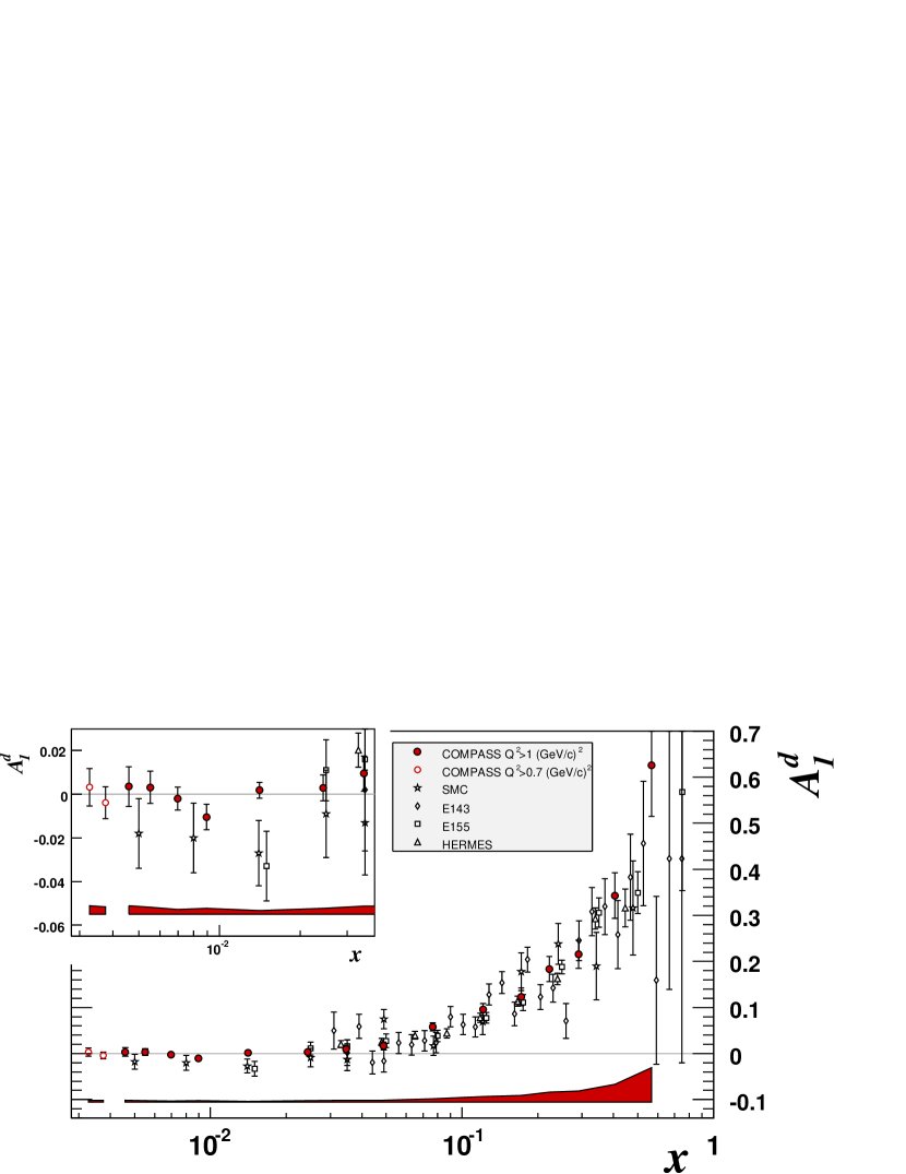
Figure 3: The asymmetry $A_{1}^{d}(x)$ as measured in COMPASS and previous results from SMC [5], HERMES [4], SLAC E143 [2] and E155 [3] at $Q^{2}>1(\mathrm{GeV}/c)^{2}$. The SLAC values of $g_{1}/F_{1}$ have been converted to $A_{1}$ and the E155 data corresponding to the same $x$ have been averaged over $Q^{2}$. Only statistical errors are shown with the data points. The shaded areas show the size of the COMPASS systematic errors.

The final values of $A_{1}^{d}(x,Q^{2})$, obtained as weighted averages of the asymmetries in the inclusive and hadronic data sets, are listed in Table 1 with the corresponding average values of $x$ and $Q^{2}$. They are also shown as a function of $x$ in Fig. 3 in comparison with previous results from experiments at CERN [5], DESY [4] and SLAC [2, 3]. The values of $A_{1}^{d}$ confirm, with increased statistical precision, the observation made in Ref. [6] that the asymmetry is consistent with zero for $x<0.03$. Values of $A_{1}^{d}$ originating from experiments at different energies tend to coincide due to the very small $Q^{2}$ dependence of $A_{1}^{d}$ at fixed $x$.

The systematic error of $A_{1}^{d}$ contains multiplicative factors resulting from uncertainties on $P_{B}$ and $P_{T}$, on the dilution factor $f$ and on the ratio $R=\sigma^{L}/\sigma^{T}$ used to calculate the depolarisation factor $D$. When combined in quadrature, these errors result in a global scale uncertainty of 10% (Table 2). The other important contribution to the systematic error is due to false asymmetries which could be generated by instabilities in some components of the spectrometer. In order to minimize their effect, the values of $A_{1}^{d}$ in each interval of $x$ have been calculated for 184 subsamples, each of them covering a short period of running time and, therefore, ensuring similar detector operating conditions. An upper limit of the effect of detector instabilities has been evaluated by a statistical approach. The dispersion of the values of $A_{1}^{d}$ around their mean agrees with the statistical error. There is thus no evidence for any broadening due to time dependent effects. Allowing the dispersion of $A_{1}^{d}$ to vary within its two standard deviations we obtain an upper limit for the systematic error of $A_{1}^{d}$ in terms of its statistical precision: $\sigma_{syst}<0.4\sigma_{stat}$. This estimation accounts for the time variation effects of spectrometer components.

Several other searches for false asymmetries were performed. Data from the two target cells were combined in different ways in order to eliminate the physical asymmetry. Data obtained with different settings of the microwave frequencies, used to polarise the target by dynamic nuclear polarisation, were compared. No evidence was found for any significant apparatus induced asymmetry.

The longitudinal spin structure function is obtained as

$$g_{1}^{d}=\frac{F_{2}^{d}}{2~{}x~{}(1+R)}A_{1}^{d}\,,$$ (4)

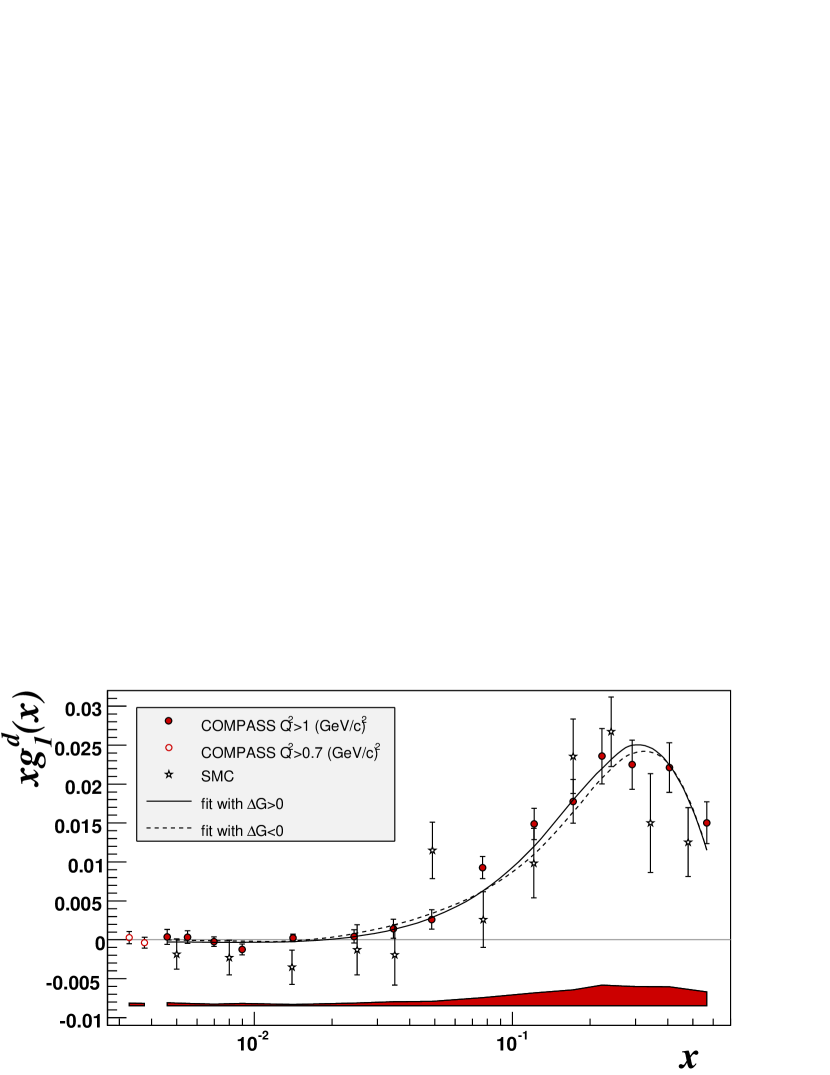
Figure 4: Values of $xg_{1}^{d}(x)$. The COMPASS points are given at the $\langle Q^{2}\rangle$ where they were measured. The SMC points have been moved to the $Q^{2}$ of the corresponding COMPASS points. Only statistical errors are shown with the data points. The shaded band at the bottom shows the COMPASS systematic error. The curves show the results of QCD fits with $\Delta G>0$ and $\Delta G<0$.

where $F_{2}^{d}$ is the spin-independent deuteron structure function. The values of $g_{1}^{d}$ listed in the last column of Table 1 have been calculated with the $F_{2}^{d}$ parametrisation of Ref. [5], which covers the range of our data, and the new parametrisation of $R$ already used in the depolarisation factor. The systematic errors on $g_{1}^{d}$ are obtained in the same way as for $A_{1}^{d}$, with an additional contribution from the uncertainty on $F_{2}^{d}$. The values of $x$, $g_{1}^{d}(x)$ for the COMPASS data and, for comparison, the SMC results [5] moved to the $Q^{2}$ of the corresponding COMPASS point are shown in Fig. 4. The two curves on the figure represent the results of two QCD fits at NLO, described below, at the measured $Q^{2}$ of each data point.

The evaluation of the first moment $\Gamma_{1}^{d}(Q^{2})=\int_{0}^{1}g_{1}^{d}(x,Q^{2})dx$ requires the evolution of all $g_{1}$ measurements to a common $Q_{0}^{2}$. This is done by using a fitted parametrisation $g_{1}^{fit}(x,Q^{2})$, so that

$$g_{1}(x,Q_{0}^{2})=g_{1}(x,Q^{2})+\Bigl{[}g_{1}^{fit}(x,Q_{0}^{2})-g_{1}^{fit}(x,Q^{2})\Bigr{]}.$$ (5)

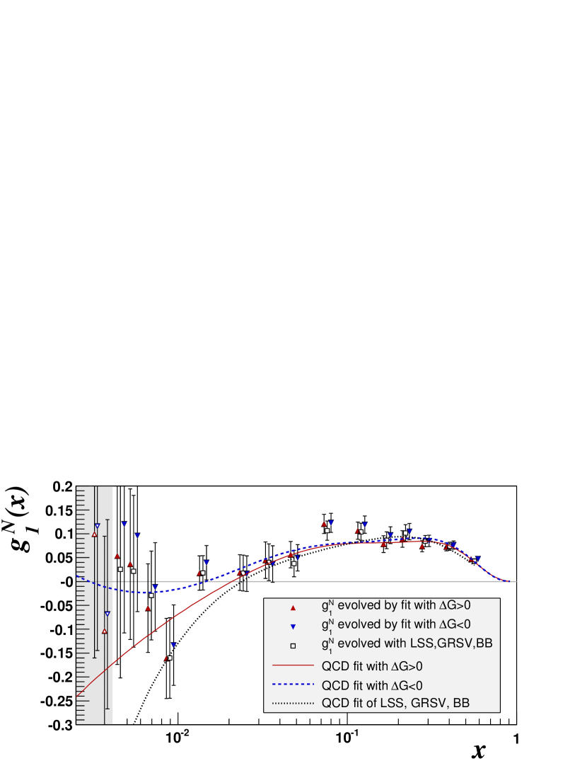
Figure 5: The COMPASS values of $g_{1}^{N}$ evolved to $Q^{2}=3(\mathrm{GeV}/c)^{2}$. The open triangles at low $x$ correspond to $Q^{2}>0.7(\mathrm{GeV}/c)^{2}$, the other symbols to $Q^{2}>1(\mathrm{GeV}/c)^{2}$. Results of QCD fits are shown by curves. In addition to our fits ($\Delta G>0$ and $\Delta G<0$) the curve obtained with three published polarised PDF parameterizations (Blümlein and Böttcher, GRSV and LSS05) [15] is shown. These parameterizations lead almost to the same values of $g_{1}^{N}\left(x,Q^{2}=3(\mathrm{GeV}/c)^{2}\right)$ and have been averaged. For clarity the data points evolved with different fits are shifted in $x$ with respect to each other. Only statistical errors are shown.

We have used several fits of $g_{1}$ from the Durham data base [15]: Blümlein-Böttcher [16], GRSV [17] and LSS05 [18], and we have chosen $Q^{2}_{0}=3(\mathrm{GeV}/c)^{2}$ as reference $Q^{2}$ because it is close to the average $Q^{2}$ of the COMPASS DIS data. The three parametrisations are quite similar in the range of the COMPASS data and have been averaged. The resulting values of $g_{1}^{N}=(g_{1}^{p}+g_{1}^{n})/2$ are shown as open squares in Fig. 5. For clarity we now use $g_{1}^{N}$ instead of $g_{1}^{d}$ because the correction for the D-wave state of the deuteron has been applied:

$$g_{1}^{N}(x,Q^{2})=g_{1}^{d}(x,Q^{2})/(1-1.5\omega_{D})$$ (6)

with $\omega_{D}=0.05\pm 0.01$ [19]. It can also be seen in Fig. 5 that the curve representing the average of the three fits does not reproduce the trend of our data for $x<0.02$ and therefore cannot be used to estimate the unmeasured part of $g_{1}^{N}$ at low $x$.

In view of this, we have performed a new NLO QCD fit of all $g_{1}$ data at $Q^{2}>1$ (GeV$/c)^{2}$ from proton, deuteron and ³He targets, including the COMPASS data. The deuteron data are from Refs. [5, 2, 3, 4], the proton data from Refs. [20, 5, 2, 21, 4] and the ³He data from Refs. [22, 23, 24, 25].

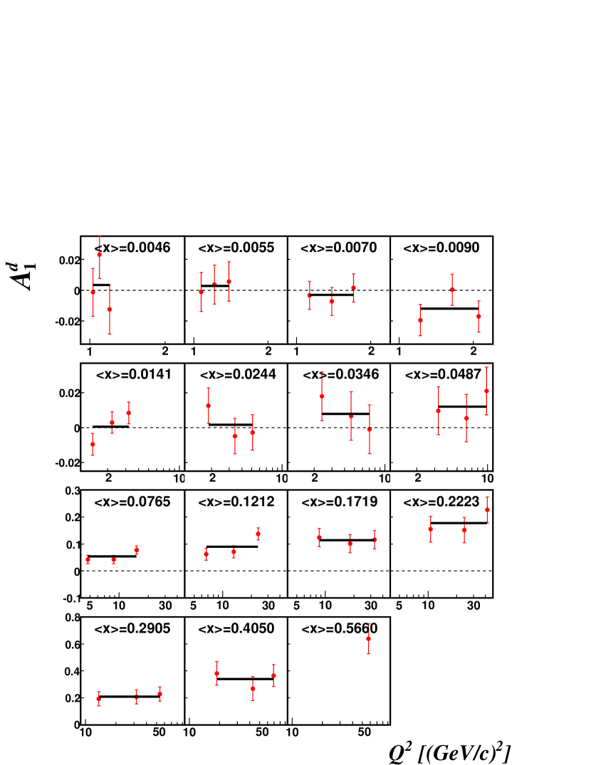
Figure 6: Values of $A_{1}^{d}$ as a function of $Q^{2}$ in intervals of $x$. The solid lines show the results of fits to a constant.

In order to optimise the use of the COMPASS data in this fit, all $x$ bins of Table 1, except the last one, have been subdivided into three $Q^{2}$ intervals (Fig. 6). The number of COMPASS data points used in the fit is thus 43, out of a total of 230.

The fit is performed in the $\overline{\rm MS}$ renormalisation and factorisation scheme and requires parametrisations of the quark singlet spin distribution $\Delta\Sigma(x)$, non-singlet distributions $\Delta q_{3}(x)$, $\Delta q_{8}(x)$ and the gluon spin distribution $\Delta G(x)$. These distributions are given as an input at a reference $Q^{2}$ ($=Q^{2}_{0}$) which is set to 3 (GeV$/c)^{2}$ and evolved according to the DGLAP equations. The resulting values of $g_{1}(x,Q^{2})$ are calculated for the $(x_{i},Q_{i}^{2})$ of each data point and compared to the experimental values.

The input parametrisations are written as

$$\Delta F_{k}=\eta_{k}\frac{x^{\alpha_{k}}\,(1-x)^{\beta_{k}}\,(1+\gamma_{k}x)}{\int_{0}^{1}x^{\alpha_{k}}\,(1-x)^{\beta_{k}}\,(1+\gamma_{k}x)dx}\,,$$ (7)

where $\Delta F_{k}$ represents each of the polarised parton distribution functions $\Delta\Sigma$, $\Delta q_{3}$, $\Delta q_{8}$ and $\Delta G$, and $\eta_{k}$ is the integral of $\Delta F_{k}$. The moments, $\eta_{k}$, of the non-singlet distributions $\Delta q_{3}$ and $\Delta q_{8}$ are fixed by the baryon decay constants ($\rm F$$+$$\rm D$) and ($\rm 3F$$-$$\rm D$) respectively, assuming SU(3)_f flavour symmetry. The linear term $\gamma x$ is used only for the singlet distribution, in which case the exponent $\beta_{G}$ is fixed because it is poorly constrained by the data. This leaves 10 parameters in the input distributions. In addition, the normalisation of E155 proton data is allowed to vary within the limits quoted by the authors of Ref. [21].

The optimal values of the parameters are obtained by minimizing the sum

$$\chi^{2}=\sum_{i=1}^{{N=230}}\frac{\Bigl{[}g_{1}^{{fit}}(x_{i},Q^{2}_{i})-g_{1}^{exp}(x_{i},Q^{2}_{i})\Bigr{]}^{2}}{\Bigl{[}\sigma(x_{i},Q^{2}_{i})\Bigr{]}^{2}}\,.$$ (8)

Here the errors $\sigma$ are the statistical ones for all data sets, except for the proton data of E155 where the uncorrelated part of the systematic error on each point is added in quadrature to the statistical one. In order to keep the parameters in their physical range, the polarised strange sea distribution $\Delta s(x)+\Delta{\overline{s}(x)}=(1/3)(\Delta\Sigma(x)-\Delta q_{8}(x))$ is calculated at every step and required to satisfy the positivity condition $\mid\Delta s(x)\mid\leq s(x)$ at all $Q^{2}$ values. A similar condition is imposed on the gluon spin distribution $\Delta G(x)$. The unpolarised distributions $s(x)$ and $G(x)$ used in this test are taken from the MRST parametrisation [26]. This procedure leads to asymmetric errors on the parameters when the fitted value is close to the allowed limit.

The fits have been performed with two different programs: the first one uses the DGLAP evolution equations for the spin structure functions [27], the other one, referred to in [28], uses the evolution of moments. The fitted PDF parameters are compatible within one standard deviation and the two programs give the same $\chi^{2}$-probabilities. In each program the $\chi^{2}$ minimisation converges to two different solutions, depending on the sign of the initial value of the gluon first moment $\eta_{G}$: one solution with $\Delta G>0$, the other one with $\Delta G<0$ (Fig. 5). The fitted distributions of $g_{1}^{N}(x)$ differ at low $x$ but are both compatible with the data. The two additional data points at $x<0.004$ and $Q^{2}>0.7(\mathrm{GeV}/c)^{2}$, not used in the fit, have too large statistical errors to provide a discrimination between the two solutions. The values of the parameters obtained in the fits with positive and negative $\Delta G$ are listed in Table 3 with their statistical errors and will be discussed below.

The integral of $g_{1}^{N}$ in the measured region is obtained from the experimental values evolved to a fixed $Q^{2}$ and averaged over the two fits. Taking into account the contributions from the fits in the unmeasured regions at low and high $x$ we obtain (Table 4):

$$\Gamma_{1}^{N}\left(Q^{2}=3(\mathrm{GeV}/c)^{2}\right)=0.050\pm 0.003\ \mbox{(stat.)}\pm 0.003\ \mbox{(evol.)}\pm 0.005\ \mbox{(syst.)}.$$ (9)

The second error accounts for the difference in $Q^{2}$ evolution between the two fits. The systematic error is the dominant one and mainly corresponds to the 10% scale uncertainty resulting from the errors on the beam and target polarisations and on the dilution factor.

For comparison, the SMC result [5] was

$$\Gamma_{1\mbox{, \sc smc}}^{N}\left(Q^{2}=10(\mathrm{GeV}/c)^{2}\right)=0.021\pm 0.007\ \mbox{(stat.)}\pm 0.014\ \mbox{(evol.)}\pm 0.003\ \mbox{(syst.)}.$$ (10)

while our result evolved to $Q^{2}=10(\mathrm{GeV}/c)^{2}$ is $0.051\pm 0.003\ \mbox{(stat.)}\pm 0.003\ \mbox{(evol.)}\pm 0.005\ \mbox{(syst.)}$. The difference between these two results reflects the fact that the COMPASS data do not support the fast decrease of $g_{1}^{d}\left(x,Q_{0}^{2}=3(\mathrm{GeV}/c)^{2}\right)$ at low $x$ which was assumed in the SMC analysis, and thus force the fit to be different. In the COMPASS analysis, the part of $\Gamma_{1}^{N}$ obtained from the measured region represents 98% of the total value. This correction of only 2% has to be compared to a correction of about 50% with respect to the measured value in case of the SMC analysis [5].

$\Gamma_{1}^{N}$ is of special interest because it gives access to the matrix element of the singlet axial current $a_{0}$ which, except for a possible gluon contribution, measures the quark spin contribution to the nucleon spin. At NLO, the relation between $\Gamma_{1}^{N}$ and $a_{0}$ reduces to

$$\Gamma_{1}^{N}(Q^{2})=\frac{1}{9}\Bigl{(}1-\frac{\alpha_{s}(Q^{2})}{\pi}+{\cal O}(\alpha_{s}^{2})\Bigr{)}\Bigl{(}a_{0}(Q^{2})+\frac{1}{4}a_{8}\Bigr{)}.$$ (11)

From the COMPASS result on $\Gamma_{1}^{N}$ (Eq. (9)) and taking the value of $a_{8}$ from hyperon $\beta$ decay, assuming $SU(3)_{f}$ flavour symmetry ($a_{8}=0.585\pm 0.025$ [29]), one obtains with the value of $\alpha_{s}$ evolved from the PDG value $\alpha_{s}(m_{Z}^{2})=0.1187\pm 0.005$ and assuming three active quark flavours:

$$a_{0}\left(Q^{2}=3(\mathrm{GeV}/c)^{2}\right)=0.35\pm 0.03\ \mbox{(stat.)}\pm 0.05\ \mbox{(syst.)}.$$ (12)

The quoted systematic error accounts for the error from the evolution and for the experimental systematic error, combined in quadrature.

The relation between $\Gamma_{1}^{N}$ and $a_{0}$ can also be rewritten in order to extract the value of the matrix element $a_{0}$ in the limit $Q^{2}\rightarrow\infty$. Here we will follow a notation of Ref. [30] introducing a “hat” for the coefficient $C^{S}_{1}$ and $a_{0}$ at this limit:

$$\Gamma_{1}^{N}(Q^{2})=\displaystyle\frac{1}{9}~{}\hat{C}^{S}_{1}(Q^{2})~{}\hat{a}_{0}~{}+~{}\frac{1}{36}~{}C^{NS}_{1}(Q^{2})~{}a_{8}.$$

The coefficients $\hat{C}_{1}^{S}$ and $C_{1}^{NS}$ have been calculated in perturbative QCD up to the third order in $\alpha_{s}(Q^{2})$ [30]:

$$\hat{C}^{S}_{1}(Q^{2})=1-0.33333\Bigl{(}{\frac{\alpha_{s}}{\pi}}\Bigr{)}-0.54959\Bigl{(}{\frac{\alpha_{s}}{\pi}}\Bigr{)}^{2}-4.44725\Bigl{(}{\frac{\alpha_{s}}{\pi}}\Bigr{)}^{3}$$

$$C^{NS}_{1}(Q^{2})=1-\Bigl{(}{\frac{\alpha_{s}}{\pi}}\Bigr{)}-3.5833\Bigl{(}{\frac{\alpha_{s}}{\pi}}\Bigr{)}^{2}-20.2153\Bigl{(}{\frac{\alpha_{s}}{\pi}}\Bigr{)}^{3}.$$

With $\alpha_{s}$ evolved at the same order, one obtains

$$\hat{a}_{0}=0.33\pm 0.03\ \mbox{(stat.)}\pm 0.05\ \mbox{(syst.)}.$$ (13)

It should be noted here that the data have been evolved to a common $Q^{2}$ on the basis of a fit at NLO only. However, the choice of a value close to the average $Q^{2}$ of the data is expected to minimise the effect of the evolution on the result quoted above. Combining this value with $a_{8}$, the first moment of the strange quark spin distribution in the limit $Q^{2}\rightarrow\infty$ is found to be

$$(\Delta s+\Delta{\overline{s}})_{Q^{2}\rightarrow\infty}=\frac{1}{3}(\hat{a}_{0}-a_{8})=-0.08\pm 0.01\ \mbox{(stat.)}\pm 0.02\ \mbox{(syst.)}.$$ (14)

As stated before, this result relies on $SU(3)_{f}$ flavour symmetry. A 20% symmetry breaking, which is considered as a maximum [29], would shift the value of $\Delta s+\Delta{\overline{s}}$ by $\pm$ 0.04.

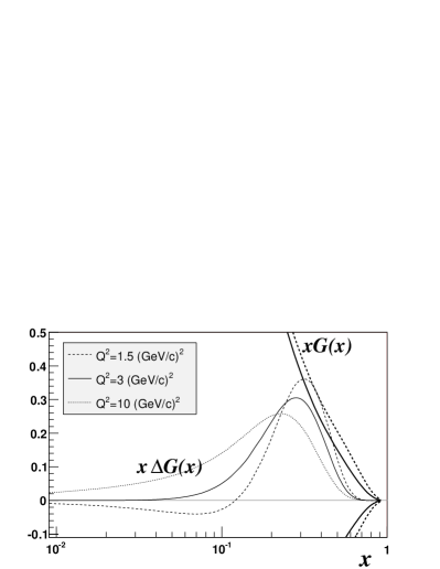
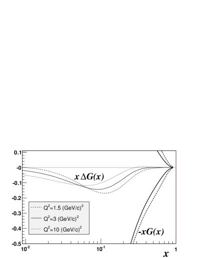
Figure 7: Gluon distribution $x\Delta G(x)$ corresponding to the fits with $\Delta G>0$ (left) and $\Delta G<0$ (right) obtained with the program of Ref. [27]. The dashed, solid and dotted lines correspond to $Q^{2}=1.5$, 3 and 10 (GeV$/c)^{2}$, respectively. The unpolarised distributions $\pm x\,G(x)$ which were used in the fit as constrains for the polarised ones are shown for $Q^{2}=1.5$ and 3 (GeV$/c)^{2}$.

Previous fits of $g_{1}$, not including the COMPASS data, found a positive $\Delta G(x)$ and a fitted function $g_{1}^{d}(x)$ becoming negative for $x\lesssim 0.025$ at $Q^{2}=3(\mathrm{GeV}/c)^{2}$, as shown by the dotted line in Fig. 5. The new COMPASS data do not reveal any evidence for a decrease of the structure function at limit $x\rightarrow 0$. For our fit the data are still compatible with a positive $\Delta G$, as shown by the full line in Fig. 5. However in this case a dip at $x\simeq 0.25$ appears in the shape of $g_{1}^{d}(x)$ for $Q^{2}\rightarrow 1(\mathrm{GeV}/c)^{2}$. Its origin is related to the shape of the fitted $\Delta G(x)$, shown in Fig. 7 (left). Indeed, the gluon spin distribution must be close to zero at low $x$, to avoid pushing $g_{1}^{d}$ down to negative values, and is also strongly limited at higher $x$ by the positivity constraint $|\Delta G(x)|<G(x)$. The whole distribution is thus squeezed in a narrow interval around the maximum at $x\simeq\alpha_{G}/(\alpha_{G}+\beta_{G})\simeq 0.25$.

In contrast, the fit with negative $\Delta G$ reproduces very well the COMPASS low $x$ data with a much smoother distribution of $\Delta G(x)$ (dashed line on Fig. 5) and without approaching the positivity limit (Fig. 7, right). The $(1+\gamma x)$ factor in the singlet quark distribution is not used in this case because it does not improve the confidence level of the fit.

Comparing the fitted parameters for $\Delta G$ positive and negative (Table 3), we observe that the parameters of the non-singlet distributions $\Delta q_{3}(x)$ and $\Delta q_{8}(x)$ are practically identical. The value of $\eta_{\Sigma}$ is slightly larger in the fit with $\Delta G<0$, as could be expected since in this case $\Delta\Sigma(x)$ remains positive over the full range of $x$:

$$\eta_{\Sigma}\left(Q^{2}=3(\mathrm{GeV}/c)^{2}\right)=0.27\pm 0.01\ \mbox{(stat.)}~{}(\Delta G>0),$$ (15)

$$\eta_{\Sigma}\left(Q^{2}=3(\mathrm{GeV}/c)^{2}\right)=0.32\pm 0.01\ \mbox{(stat.)}~{}(\Delta G<0).$$ (16)

We remind that in $\overline{\mbox{MS}}$ scheme $\eta_{\Sigma}$ is identical to the matrix element $a_{0}$.

The singlet moment derived from the fits to all $g_{1}$ data is thus:

$$\eta_{\Sigma}\left(Q^{2}=3(\mathrm{GeV}/c)^{2}\right)=0.30\pm 0.01\ \mbox{(stat.)}\pm 0.02\ \mbox{(evol.)}.$$ (17)

Here we have taken the difference between the fits as an estimate of the systematic error and do not further investigate other contributions related to the choice of the QCD scale or the PDF parametrisations. The singlet moment obtained with COMPASS data alone (Eq. (12)) is slightly above this value and its statistical error is larger by a factor of 3. As stated before, the main uncertainty on the COMPASS result is due to the 10% normalisation uncertainty from the beam and target polarisations and from the dilution factor. The fact that the COMPASS data are on average slightly above the world average can already be detected by a comparison of the measured $g_{1}^{d}$ values to the curves fitted to the world data (Fig. 5). Hence $a_{0}$ derived from the COMPASS value of $\Gamma_{1}^{N}$ is found to be slightly larger than $\eta_{\Sigma}$.

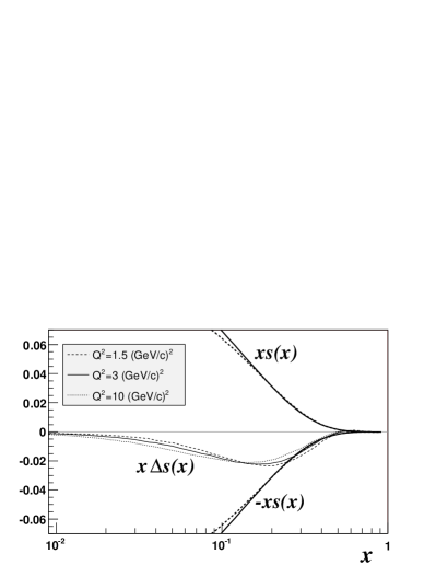
Figure 8: Strange quark distribution $x\Delta s(x)$ corresponding to the fits with $\Delta G>0$ (left) and $\Delta G<0$ (right) obtained with the program of Ref. [27]. The dashed, solid and dotted lines correspond to $Q^{2}=1.5$, 3 and 10 (GeV$/c)^{2}$, respectively. The unpolarised distributions $\pm x\,s(x)$ are shown for $Q^{2}=1.5$ and 3 (GeV$/c)^{2}$.

The polarised strange quark distributions, obtained from the difference between $\Delta\Sigma(x)$ and $\Delta q_{8}(x)$ are shown in Fig. 8. They are negative and concentrated in the highest $x$ region, compatible with the constraint $|\Delta s(x)|<s(x)$. This condition is indeed essential in the determination of the $\Delta q_{8}$ parameters which otherwise would be poorly constrained.

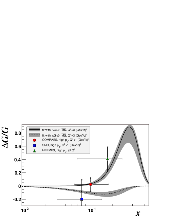
Figure 9: Distribution of the gluon polarisation $\Delta G(x)/G(x)$ at $Q^{2}=3(\mathrm{GeV}/c)^{2}$ for the fits with $\Delta G>0$ and $\Delta G<0$ obtained with the program of Ref. [27]. The error bands correspond to the statistical error on $\Delta G(x)$ at a given $x$. The unpolarised gluon distribution is taken from the MRST parametrisation [26]. The three data points show the measured values from SMC [31], HERMES [32] and COMPASS [33]. Two error bars are associated to each data point, one corresponding to the statistical precision and the other one to the statistical and systematic errors added in quadrature. The horizontal bar on each point shows the $x$-range of measurement.

Although the gluon distributions strongly differ in the two fits, the fitted values of their first moments are both small and about equal in absolute value $|\eta_{G}|\approx 0.2-0.3$. We have also checked the stability of these results with respect to a change in $\alpha_{s}(m_{Z}^{2})$: when $\alpha_{s}(m_{Z}^{2})$ is varied by $\pm 0.005$ the values of $\eta_{G}$ are not changed by more than half a standard deviation. In Fig. 9 the existing direct measurements of $\Delta G/G$ [31, 32, 33] are shown with the distributions of $\Delta G(x)/G(x)$ derived from our fits with $G(x)$ taken from Ref. [26]. The HERMES value is positive and $2\sigma$ away from zero. The measured SMC point is too unprecise to discriminate between positive or negative $\Delta G$. The published COMPASS point, which has been obtained from a partial data sample corresponding to about 40% of the present statistics, is almost on the $\Delta G>0$ curve but is only $1.3\sigma$ away from the $\Delta G<0$ one, so that no preference for any of the curves can be given so far. It should also be noted that the measured values of $\Delta G/G$ have all been obtained in leading order QCD analyses.

In summary, we have measured the deuteron spin asymmetry $A_{1}^{d}$ and its longitudinal spin-dependent structure function $g_{1}^{d}$ with improved precision at $Q^{2}>1(\mathrm{GeV}/c)^{2}$ over the range $0.004<x<0.70$. The $g_{1}^{d}$ values are consistent with zero for $x<0.03$. The measured values have been evolved to a common $Q^{2}$ by a new fit of the world $g_{1}$ data, and the first moment $\Gamma_{1}^{N}$ has been evaluated at $Q^{2}=3(\mathrm{GeV}/c)^{2}$ with a statistical error smaller than 0.003. From $\Gamma_{1}^{N}$ we have derived the matrix element of the singlet axial current $\hat{a}_{0}$ in the limit $Q^{2}\rightarrow\infty$. With COMPASS data alone, at the order $\alpha_{s}^{3}$, it has been found that $\hat{a}_{0}=0.33\pm 0.03\ \mbox{(stat.)}\pm 0.05\ \mbox{(syst.)}$ and the first moment of the strange quark distribution $(\Delta s+\Delta{\overline{s}})_{Q^{2}\rightarrow\infty}=-0.08\pm 0.01\ \mbox{(stat.)}\pm 0.02\ \mbox{(syst.)}$. We also observe that the fit of world $g_{1}$ data at NLO yields two solutions with either $\Delta G(x)>0$ or $\Delta G(x)<0$, which equally well describe the present data. In both cases, the first moment of $\Delta G(x)$ is of the order of 0.2–0.3 in absolute value at $Q^{2}=3(\mathrm{GeV}/c)^{2}$ but the shapes of the distributions are very different.

$x$ range	$\langle x\rangle$	$\langle Q^{2}\rangle$	$A_{1}^{d}$	$g_{1}^{d}$
		[(GeV$/c)^{2}]$
0.0030–0.0035	0.0033	0.78	$0.003\pm 0.009\pm 0.004$	$0.090\pm 0.240\pm 0.107$
0.0035–0.0040	0.0038	0.83	$-0.004\pm 0.007\pm 0.003$	$-0.097\pm 0.183\pm 0.082$
0.004–0.005	0.0046	1.10	$0.004\pm 0.009\pm 0.004$	$0.082\pm 0.210\pm 0.089$
0.005–0.006	0.0055	1.22	$0.003\pm 0.007\pm 0.003$	$0.062\pm 0.146\pm 0.062$
0.006–0.008	0.0070	1.39	$-0.002\pm 0.005\pm 0.002$	$-0.034\pm 0.086\pm 0.036$
0.008–0.010	0.0090	1.61	$-0.010\pm 0.006\pm 0.003$	$-0.139\pm 0.078\pm 0.035$
0.010–0.020	0.0141	2.15	$0.002\pm 0.004\pm 0.002$	$0.017\pm 0.033\pm 0.014$
0.020–0.030	0.0244	3.18	$0.003\pm 0.006\pm 0.003$	$0.017\pm 0.035\pm 0.015$
0.030–0.040	0.0346	4.26	$0.009\pm 0.008\pm 0.004$	$0.041\pm 0.035\pm 0.016$
0.040–0.060	0.0487	5.80	$0.017\pm 0.008\pm 0.004$	$0.054\pm 0.026\pm 0.012$
0.060–0.100	0.0765	8.53	$0.058\pm 0.009\pm 0.007$	$0.121\pm 0.019\pm 0.014$
0.100–0.150	0.121	12.6	$0.095\pm 0.013\pm 0.011$	$0.123\pm 0.017\pm 0.014$
0.150–0.200	0.171	17.2	$0.123\pm 0.020\pm 0.014$	$0.103\pm 0.016\pm 0.012$
0.200–0.250	0.222	21.8	$0.183\pm 0.028\pm 0.021$	$0.106\pm 0.016\pm 0.012$
0.250–0.350	0.290	28.3	$0.216\pm 0.030\pm 0.024$	$0.077\pm 0.011\pm 0.009$
0.350–0.500	0.405	39.7	$0.343\pm 0.049\pm 0.038$	$0.055\pm 0.008\pm 0.006$
0.500–0.700	0.566	55.3	$0.626\pm 0.112\pm 0.075$	$0.027\pm 0.005\pm 0.003$

Table 1: Values of $A_{1}^{d}$ and $g_{1}^{d}$ with their statistical and systematical errors as a function of $x$ with the corresponding average values of $x$ and $Q^{2}$. The minimum $Q^{2}$ cut is 1 (GeV$/c)^{2}$ except for the first two points where it is lowered to 0.7 (GeV$/c)^{2}$. These two data points are shown on the figures as complementary information but were not used in the fits.

	Beam polarization	$dP_{B}/P_{B}$	5%
Multiplicative	Target polarization	$dP_{T}/P_{T}$	5%
variables	Depolarization factor	$dD(R)/D(R)$	2 – 3 %
error, $\Delta A_{1}^{mult}$	Dilution factor	$df/f$	6 %
	Total		$\Delta A_{1}^{mult}\simeq 0.1A_{1}$
Additive	Transverse asymmetry	${\eta}/\rho\cdot\Delta A_{2}$	$10^{-4}-5\cdot 10^{-3}$
variables	Radiative corrections	$\Delta A_{1}^{RC}$	$10^{-4}-10^{-3}$
error, $\Delta A_{1}^{add}$	False asymmetry	$A_{false}$	$<0.4\cdot\Delta A_{1}^{stat}$

Table 2: Decomposition of the systematic error of $A_{1}$ into multiplicative and additive variables contributions.

$\Delta G>0$
	Prog. Ref. [27]	Prog. Ref. [28]
$\eta_{\Sigma}$	$0.270\pm 0.014$	$0.284~{}^{+~{}0.016}_{-~{}0.014}$
$\alpha_{\Sigma}$	$-0.303~{}^{+~{}0.074}_{-~{}0.079}$	$-0.226~{}^{+~{}0.103}_{-~{}0.101}$
$\beta_{\Sigma}$	$3.60^{+~{}0.24}_{-~{}0.22}$	$3.69~{}^{+~{}0.30}_{-~{}0.25}$
$\gamma_{\Sigma}$	$-16.0~{}^{+~{}1.4}_{-~{}1.6}$	$-15.8~{}^{+~{}1.7}_{-~{}2.8}$
$\eta_{G}$	$0.336^{+~{}0.049}_{-~{}0.070}$	$0.233~{}^{+~{}0.040}_{-~{}0.053}$
$\alpha_{G}$	$2.91^{+~{}0.40}_{-~{}0.44}$	$3.11^{+~{}0.42}_{-~{}0.53}$
$\beta_{G}$	$10$ (fixed)	$10$ (fixed)
$\alpha_{3}$	$-0.226\pm 0.027$	$-0.226~{}^{+~{}0.029}_{-~{}0.027}$
$\beta_{3}$	$2.43^{+~{}0.11}_{-~{}0.10}$	$2.38~{}^{+~{}0.11}_{-~{}0.10}$
$\alpha_{8}$	$0.35^{+~{}0.18}_{-~{}0.44}$	$0.45~{}^{+~{}0.13}_{-~{}0.43}$
$\beta_{8}$	$3.36^{+~{}0.60}_{-~{}1.04}$	$3.50~{}^{+~{}0.46}_{-~{}0.98}$
$\chi^{2}/{\rm ndf}$	233/219	232/219

$\Delta G<0$
	Prog. Ref. [27]	Prog. Ref. [28]
$\eta_{\Sigma}$	$0.320\pm 0.009$	$0.328\pm 0.009$
$\alpha_{\Sigma}$	$1.38^{+~{}0.15}_{-~{}0.14}$	$1.38~{}^{+~{}0.13}_{-~{}0.12}$
$\beta_{\Sigma}$	$4.08^{+~{}0.29}_{-~{}0.27}$	$4.05~{}^{+~{}0.25}_{-~{}0.23}$
$\gamma_{\Sigma}$	-	-
$\eta_{G}$	$-0.309^{+~{}0.095}_{-~{}0.144}$	$-0.192~{}^{+~{}0.064}_{-~{}0.109}$
$\alpha_{G}$	$0.39^{+~{}0.65}_{-~{}0.48}$	$0.23~{}^{+0.063}_{-~{}0.47}$
$\beta_{G}$	$13.9^{+~{}7.8}_{-~{}5.4}$	$13.8~{}^{+~{}8.2}_{-~{}5.6}$
$\alpha_{3}$	$-0.212\pm 0.027$	$-0.209\pm 0.027$
$\beta_{3}$	$2.44^{+~{}0.11}_{-~{}0.10}$	$2.40~{}^{+~{}0.11}_{~{}-0.10}$
$\alpha_{8}$	$0.43~{}^{+~{}0.15}_{-~{}0.16}$	$0.383~{}^{+~{}0.080}_{-~{}0.121}$
$\beta_{8}$	$3.54^{+~{}0.55}_{-~{}0.54}$	$3.39~{}^{+~{}0.33}_{-~{}0.39}$
$\chi^{2}/{\rm ndf}$	247/219	247/219

	$\eta_{\Sigma}$	$\alpha_{\Sigma}$	$\beta_{\Sigma}$	$\gamma_{\Sigma}$	$\eta_{G}$	$\alpha_{G}$	$\beta_{G}$	$\alpha_{3}$	$\beta_{3}$	$\alpha_{8}$	$\beta_{8}$
$\eta_{\Sigma}$		$0.581$	$0.143$	$-0.432$	$-0.548$	$0.549$	–	$-0.075$	$-0.118$	$0.030$	$-0.008$
$\alpha_{\Sigma}$	$-0.492$		$0.648$	$0.272$	$-0.434$	$0.452$	–	$0.053$	$0.066$	$-0.121$	$-0.047$
$\beta_{\Sigma}$	$-0.388$	$0.877$		$0.304$	$-0.011$	$0.022$	–	$-0.010$	$-0.037$	$-0.420$	$-0.499$
$\gamma_{\Sigma}$	–	–	–		$0.272$	$-0.248$	–	$0.088$	$0.142$	$-0.361$	$-0.025$
$\eta_{G}$	$0.277$	$-0.221$	$-0.130$	–		$-0.978$	–	$0.082$	$0.066$	$0.071$	$0.067$
$\alpha_{G}$	$0.162$	$-0.052$	$0.012$	–	$0.835$		–	$-0.087$	$-0.070$	$-0.069$	$-0.063$
$\beta_{G}$	$0.148$	$-0.039$	$0.025$	–	$0.814$	$0.935$		–	–	–	–
$\alpha_{3}$	$-0.012$	$0.008$	$-0.032$	–	$0.078$	$0.006$	$0.053$		$0.788$	$-0.023$	$-0.020$
$\beta_{3}$	$-0.104$	$0.067$	$0.037$	–	$0.060$	$0.003$	$0.023$	$0.793$		$-0.017$	$-0.013$
$\alpha_{8}$	$-0.105$	$-0.175$	$-0.276$	–	$0.171$	$0.099$	$0.219$	$-0.036$	$-0.016$		$0.832$
$\beta_{8}$	$-0.137$	$0.033$	$-0.211$	–	$0.118$	$0.063$	$0.138$	$-0.044$	$-0.026$	$0.821$

Table 3: Top: Values of the parameters obtained from the QCD analysis at $Q^{2}=3$ (GeV$/c)^{2}$ in fits with $\Delta G>0$ and $\Delta G<0$ with the two programs. The quoted errors correspond to one $\sigma$ and have been obtained from the MINOS analysis [34]. The strongly asymmetric errors obtained for some parameters are due to the positivity constraints applied in the fits. Bottom: Correlation matrices for the fits by the program of Ref. [27]. The triangles above and below the diagonal correspond to the fits with $\Delta G>0$ and $\Delta G<0$, respectively. The “–” symbols correspond to parameters which are fixed in one of the fits.

	COMPASS data evolved to $Q^{2}=3(\mathrm{GeV}/c)^{2}$ using
Range in $x$	fits of		COMPASS fits (prog. [27])
	BB[16]	LSS[18]	$\Delta G>0$	$\Delta G<0$
$[\,0.004,\,0.7\,]$	$0.0455$	$0.0469$	$0.0469$	$0.0511$
$[\,0.7,\,1\,]$	$0.0014$	$0.0008$	$0.0011$	$0.0010$
$[\,0,\,0.004\,]$	$-0.0040$	$-0.0029$	$-0.0014$	$0.0004$
$[\,0,\,1\,]$	$0.0430$	$0.0448$	$0.0466$	$0.0525$

Table 4: Contributions to $\Gamma_{1}^{N}\left(Q^{2}=3(\mathrm{GeV}/c)^{2}\right)$ from different kinematic regions. The values in the first line are the COMPASS results evolved according to different fits and integrated over the measured $x$ range. The second and third lines show the corresponding high and low $x$ extrapolations.

Figure 1: Fraction of inclusive, semi-inclusive, and calorimetric triggers as a function of $x$. Events are counted with the weight they carry in the asymmetry calculation.

Figure 2: Difference between asymmetries for inclusive and hadronic Monte Carlo events in the kinematic range covered by the purely calorimetric trigger.

References

- [1] SMC Collaboration, B. Adeva et al., Phys. Lett. B 302 (1993) 533.
- [2] E143 Collaboration, K. Abe et al., Phys. Rev. D 58 (1998) 112003.
- [3] E155 Collaboration, P. L. Anthony et al., Phys. Lett. B 463 (1999) 339.
- [4] HERMES Collaboration, A. Airapetian et al., Phys. Rev. D 71 (2005) 012003.
- [5] SMC Collaboration, B. Adeva et al., Phys. Rev. D 58 (1998) 112001.
- [6] COMPASS Collaboration, E. S. Ageev et al., Phys. Lett. B 612 (2005) 154.
- [7] C. Bernet et al., Nucl. Instrum. Methods A 550 (2005) 217.
- [8] A. A. Akhundov et al., Fortsch. Phys. 44 (1996) 373.
- [9] SMC Collaboration, D. Adams et al., Phys. Rev. D 56 (1997) 5330.
- [10] E155 Collaboration, P. L. Anthony et al., Phys. Lett. B 553 (2003) 18.
- [11] E143 Collaboration, K. Abe et al., Phys. Lett. B 452 (1999) 194.
- [12] HERMES Collaboration, A. Airapetian et al., Phys. Rev. Lett. 95 (2005) 242001.
- [13] I. V. Akushevich and N. M. Shumeiko, J. Phys. G 20 (1994) 513.
- [14] A. Bravar, K. Kurek and R. Windmolders, Comput. Phys. Commun. 105 (1997) 42.
- [15] The Durham HEP Databases, http://durpdg.dur.ac.uk/HEPDATA/pdf.html
- [16] J. Blümlein and H. Böttcher, Nucl. Phys. B 636 (2002) 225.
- [17] M. Glück, E. Reya, M. Stratmann and W. Vogelsang, Phys. Rev. D 63 (2001) 094005.
- [18] E. Leader, A. V. Sidorov and D. B. Stamenov, Phys. Rev. D 73 (2006) 034023.
- [19] R. Machleidt et al., Phys. Rep. 149 (1987) 1.
- [20] EMC Collaboration, J. Ashman et al., Nucl. Phys. B 328 (1989) 1.
- [21] E155 Collaboration, P. L. Anthony et al., Phys. Lett. B 493 (2000) 19.
- [22] E142 Collaboration, P. L. Anthony et al., Phys. Rev. D 54 (1996) 6620.
- [23] E154 Collaboration, K. Abe et al., Phys. Rev. Lett. 79 (1997) 26.
- [24] JLAB/Hall A Collaboration, X. Zheng et al., Phys. Rev. Lett. 92 (2004) 012004.
- [25] HERMES Collaboration, K. Ackerstaff et al., Phys. Lett. B 404 (1997) 383.
- [26] A. D. Martin et al., Phys. Lett. B 604 (2004) 61.
- [27] SMC Collaboration, B. Adeva et al., Phys. Rev. D 58 (1998) 112002.
- [28] A. N. Sissakian, O. Yu. Shevchenko and O. N. Ivanov, Phys. Rev. D 70 (2004) 074032.
- [29] E. Leader, D. Stamenov, Phys. Rev. D 67 (2003) 037503.
- [30] S. A. Larin et al., Phys. Lett. B 404 (1997) 153.
- [31] SMC Collaboration, B. Adeva et al., Phys. Rev. D 70 (2004) 012002.
- [32] HERMES Collaboration, A. Airapetian et al., Phys. Rev. Lett. 84 (2000) 2584.
- [33] COMPASS Collaboration, E. S. Ageev et al., Phys. Lett. B 633 (2006) 25.
- [34] F. James, MINUIT, CERN Program Library Long Writeup D506.