Dalitz plot analysis of $\mbox{$e^{+}$}\mbox{$e^{-}$}\to\mbox{$\pi^{0}$}\mbox{$\pi^{0}$}\gamma$ events at $\sqrt{s}\simeq M_{\phi}$ with the KLOE detector

Abstract

We have studied the Dalitz plot of the $\mbox{$e^{+}$}\mbox{$e^{-}$}\to\mbox{$\pi^{0}$}\mbox{$\pi^{0}$}\gamma$ events collected at $\sqrt{s}\simeq M_{\phi}$ with the KLOE detector. In the dipion invariant mass ($M_{\pi\pi}$) region below 700 MeV, the process under study is dominated by the non-resonant process $\mbox{$e^{+}$}\mbox{$e^{-}$}\to\omega\mbox{$\pi^{0}$}$ with $\omega\to\mbox{$\pi^{0}$}\gamma$ whereas, for higher $M_{\pi\pi}$ values, the radiative $\phi$ decay to the $f_{0}$(980) is the dominant mechanism. Different theoretical models are used to fit the Dalitz plot, taking also into account a possible contribution of the $\sigma(600)$. For each model, we extract the $f_{0}(980)$ mass and its coupling to $\pi\pi$, $K\overline{K}$ and to the $\phi$.

1 Introduction

Interest in light scalar mesons remains intense in hadron spectroscopy due to a lack of elucidation on their nature. There is a possibility that some of them are, in fact, exotic particles. There are several models to describe their structure, such as ordinary $q\overline{q}$ mesons, $qq\overline{qq}$ states or $K\overline{K}$ molecules Tornqvist ; Jaffe ; Molecule . Operating at the $e^{+}$$e^{-}$ Frascati $\phi$-factory DA$\Phi$NE DAFNE , the KLOE experiment KLOE is ideally suited for the study of these particles, since the radiative decays of the $\phi$ into two pseudoscalar mesons is dominated by a scalar meson ($S$) exchange in the intermediate state ($\phi\to S\gamma\to\pi\pi\gamma/\eta\pi\gamma/\mbox{$K\overline{K}$}\gamma$). For the $\mbox{$\pi^{0}$}\mbox{$\pi^{0}$}\gamma$ final state, the possible scalar contributions are from the well established $f_{0}$(980) and from the more controversial $\sigma(600)$, purportedly observed by the E791 and BES collaborations s600_E791 ; s600_BES . The non-resonant $\mbox{$e^{+}$}\mbox{$e^{-}$}\to\omega\mbox{$\pi^{0}$}\to\mbox{$\pi^{0}$}\mbox{$\pi^{0}$}\gamma$ reaction also contributes to the same final state.

The $\mbox{$\pi^{0}$}\mbox{$\pi^{0}$}\gamma$ final state had been studied at KLOE using 16 pb^-1 of 2000 data PLBf0n2002 . The resulting ratio between the $f_{0}KK$ and $f_{0}\pi\pi$ couplings, together with the large value of the BR, favoured the $qq\overline{qq}$ composition of the $f_{0}$(980), while the shape of the $\pi^{0}$$\pi^{0}$ invariant mass suggested a possible contribution also from $\sigma(600)$. In the present paper, the analysis is repeated with a statistics about thirty times larger, thus allowing us to study this reaction in much greater detail. A common set of cuts and algorithms for the resonant and non-resonant processes has been developed so that, by fitting the Dalitz plot, the differential cross sections of the two components are extracted. A detailed technical description of this analysis is in Refs. KNana ; KNfit .

2 Experimental setup

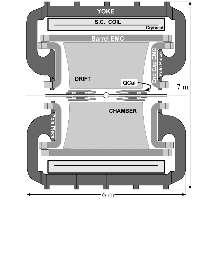
Data were collected with the KLOE detector at DA$\Phi$NE, the Frascati $e^{+}$$e^{-}$ $\phi$-factory, which operates at a center of mass energy $\mbox{$\sqrt{s}$}=M_{\phi}\sim 1020$ MeV. The beams collide with a crossing angle of $(\pi-25)$ mrad, producing $\phi$ mesons with a small momentum ($p_{\phi}\sim 13$ MeV/c) in the horizontal plane. The KLOE detector (see Fig. 1) is inserted in a 0.52 T magnetic field. It consists of a 2 m radius drift chamber (DC) DCH , with full stereo geometry using helium based gas mixture, surrounded by a fine sampling lead/scintillating fibers electromagnetic calorimeter (EMC) EMC , divided into a barrel and two endcaps, with a hermetic coverage (98% of the solid angle) and a very high efficiency for low energy photons. Since the channel $\mbox{$e^{+}$}\mbox{$e^{-}$}\to\mbox{$\pi^{0}$}\mbox{$\pi^{0}$}\gamma$ under study is fully neutral, its analysis is based mainly on the EMC performance. The arrival times of particles and the positions in three dimensions of the energy deposits are obtained from the signals collected at the two ends of the calorimeter modules, with a granularity of $\sim(4.4\times 4.4)$ cm², for a total of 2440 cells arranged in five layers. Cells close in time and space are grouped into a calorimeter cluster. The probability of a photon to fragment in more than a cluster (splitting) is reduced by employing a special recovery algorithm. The cluster energy $E$ is the sum of the cell energies, while the cluster time $T$ and its position $\vec{R}$ are energy weighted averages. Photon energy and time resolutions are $\sigma_{E}/E=5.7\%/\sqrt{E\ {\rm(GeV)}}$ and $\sigma_{T}=57\ {\rm ps}/\sqrt{E\ {\rm(GeV)}}\oplus 100\ {\rm ps}$, respectively. The KLOE trigger TRG is based on the detection of two energy deposits (called sectors) with $E>50$ MeV for barrel and $E>150$ MeV for endcaps. Events with only two fired trigger sectors in the same endcap are rejected, being this topology dominated by machine background. Recognition and rejection of cosmic-ray events is also performed at the trigger level, selecting events with two energy deposits above a 30 MeV threshold in the outermost calorimeter layer. Moreover, to reject residual cosmic rays and machine background events, an offline software filter uses calorimeter and DC information before track reconstruction NIMOffline .

Figure 1: Vertical cross section of the KLOE detector.

The machine parameters (center of mass energy $\sqrt{s}$, $\phi$ momentum and beams interaction point) are measured on-line from the analysis of Bhabha scattering events in the barrel. The average value of the center-of-mass energy is evaluated with a precision of 30 keV per run, each corresponding to $\sim 100\ \mbox{nb}^{-1}$ of integrated luminosity. To calibrate the absolute beam energy scale we fit the $\phi$ line shape of $\phi\to\eta\gamma$ events KNana . Comparing the value obtained for $M_{\phi}$ with the precise measurement of the CMD-2 experiment obtained with the depolarization method MphiCMD2 , a shift of $+150$ keV is found and is corrected in our analysis accordingly.

Prompt photons are identified as neutral particles with $\beta=1$ originated at the interaction point, by requiring $|T-R/c|<{\rm min}(5\,\sigma_{T},2\ {\rm ns})$, where $T$ is the photon flight time and $R$ the corresponding path length. The photon detection efficiency is $\sim 90\%$ for $E_{\gamma}$=20 MeV, and reaches 100% above 70 MeV. The sample selected by the timing requirement has less than $0.6\%$ contamination per event due to accidental clusters from machine background.

3 Event selection

All the available statistics collected in 2001–2002 data-taking periods, corresponding to 450 pb^-1, has been analyzed by grouping all runs in center of mass energy bins of 100 keV. This was done to take into account the $\sim 2$ MeV spread in the center of mass energy present in the data set. For this analysis, only those runs belonging to the bin with the highest statistics have been used for fitting the Dalitz plot. This sample corresponds to 145 pb^-1 collected at $\mbox{$\sqrt{s}$}=(1019.7\div 1019.8)$ MeV.

The response of the detector to the decays of interest was studied by using the KLOE Monte Carlo (MC) simulation program NIMOffline . The MC takes into account changes in the machine operation and background conditions, in order to reproduce real data on a run-by-run basis. For the present analysis, an MC sample for both signal and backgrounds is produced. The corresponding integrated luminosity is five times that of the collected data, except for $\mbox{$e^{+}$}\mbox{$e^{-}$}\to\gamma\gamma$ events that are produced at a 1:1 rate. For the simulation of signal events, the $M_{\pi\pi}$ spectrum for the $\phi\to S\gamma\to\pi\pi\gamma$ ($S\gamma$) process is produced according to the shape obtained from 2000 data, while the $\mbox{$e^{+}$}\mbox{$e^{-}$}\to\omega\mbox{$\pi^{0}$}\to\mbox{$\pi^{0}$}\mbox{$\pi^{0}$}\gamma$ ($\omega\pi$) generator is based on the Vector Meson Dominance (VMD) description of the three body decay according to Ref. SwpnSND .

The data analysis consists of four steps:

1. an acceptance selection of five prompt photons with $E_{\gamma}\geq 7$ MeV and a polar angle satisfying the requirement $|\cos\theta_{\gamma}|<0.92$;

2. a kinematic fit (Fit1) imposing total 4-momentum conservation;

3. a pairing procedure of photons to $\pi^{0}$’s, where the photon combination minimizing a pseudo-$\chi^{2}$ built using the invariant mass of the two $\gamma\gamma$ pairs, $\chi^{2}_{\rm pair}$, is selected as the good one;

4. a second kinematic fit (Fit2), where the constraints on the $\pi^{0}$ masses are also imposed. The selected events must then satisfy the requirements $\chi^{2}_{\rm Fit2}/{\rm Ndf}\leq 5$ and $\Delta M_{\gamma\gamma}=|M_{\gamma\gamma}-M_{\pi}|\leq 5\,\sigma_{\gamma\gamma}$, where $M_{\gamma\gamma}$ and $\sigma_{\gamma\gamma}$ are evaluated using the photon momenta from Fit1.

A further cut is applied to reject the background from the $\mbox{$e^{+}$}\mbox{$e^{-}$}\to\gamma\gamma$ process, which has a cross section much larger than the signal and where the three additional prompt photons could be generated either by radiation, by cluster splitting or by accidental coincidence with machine background clusters. Such process is hugely reduced without losing efficiency for the signal, by rejecting events where the energy sum of the two most energetic clusters in the event is greater than 900 MeV.

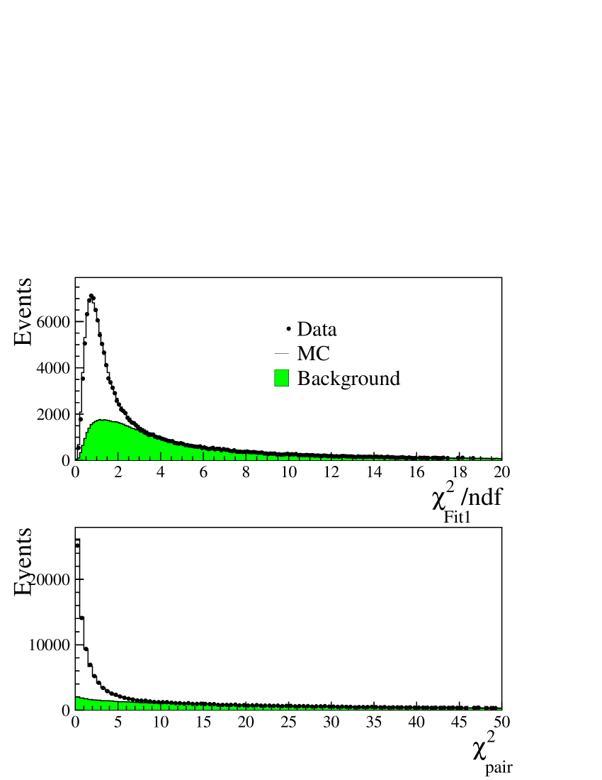
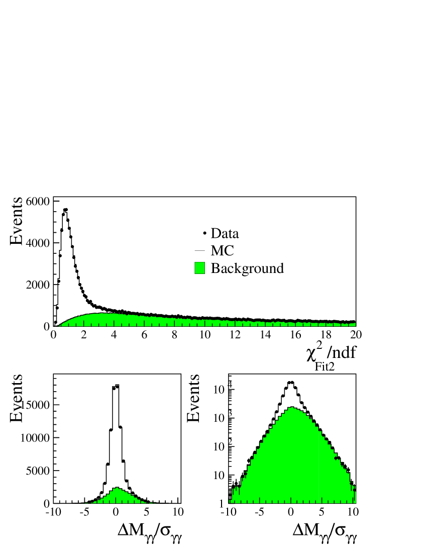
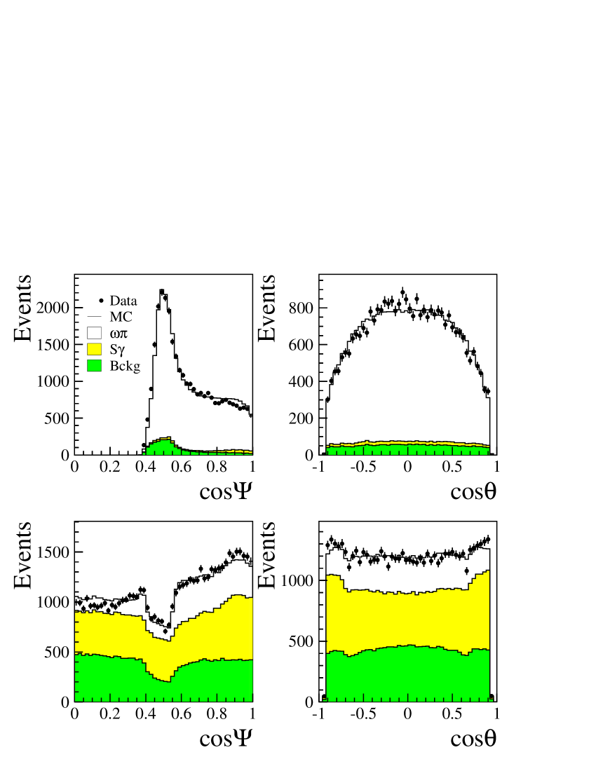
The overall analysis efficiency for the identification of the signal is evaluated by applying the whole analysis chain to the $S\gamma$ and $\omega\pi$ MC events: $\varepsilon_{S\gamma}=(50.3\pm 0.1)\%$, $\varepsilon_{\omega\pi}=(53.12\pm 0.05)\%$. The small difference is due to the characteristic energy and angular distributions of photons in the two kinds of events. After acceptance selection we start with a sample of 243,904 events of which 86,449 survive the complete analysis chain. As shown in Figs. 2, 3 excellent data-MC agreement is found, both after acceptance selection and after applying the complete analysis chain.

Figure 2: Data-MC comparison after acceptance selection: normalized $\chi^{2}$ from the first kinematic fit (top) and the minimum value of the pseudo-$\chi^{2}$ used to pair photons (bottom).

Figure 3: Top: normalized $\chi^{2}$ of the second kinematic fit after acceptance cuts. Bottom: normalized $\Delta M_{\gamma\gamma}$ of the selected $\gamma\gamma$ pairs after $\chi^{2}_{\rm Fit2}$ cut in linear (left) and logarithmic (right) scale.

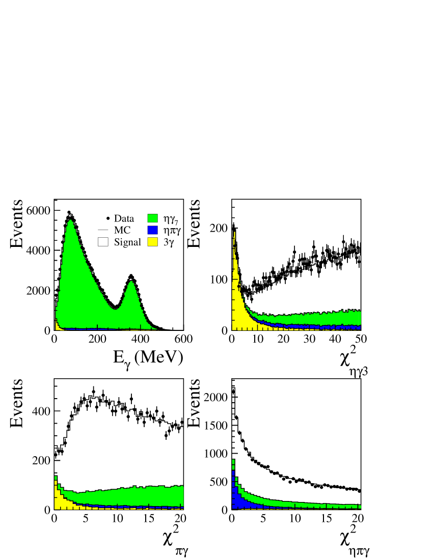
The background channels for the $\mbox{$\pi^{0}$}\mbox{$\pi^{0}$}\gamma$ final state are listed in Tab. 1 together with the analysis efficiency and the corresponding signal to background ratio, before and after the application of the analysis cuts, evaluated using branching ratios (BRs) from Ref. PDG03 or KLOE measurements whenever available PLBa0 ; eta2000 . The $\phi\to\eta\pi^{0}\gamma$ channel ($\eta\pi\gamma$) is the only one that has the same five photon final state as the signal. The $\phi\to\eta\gamma\to\mbox{$\pi^{0}$}\mbox{$\pi^{0}$}\mbox{$\pi^{0}$}\gamma$ ($\eta\gamma_{7}$) mimics the signal when there are lost or merged photons. The three photon final states ($\phi\to\eta\gamma$ [$\eta\gamma_{3}$], $\phi\to\mbox{$\pi^{0}$}\gamma$ [$\pi\gamma$] and $\mbox{$e^{+}$}\mbox{$e^{-}$}\to\gamma\gamma(\gamma)$ [$\gamma\gamma$]) produce five clusters due to splitting or accidental coincidence with clusters produced by machine background. We have used background-enriched distributions to check the absolute yields and the Monte Carlo shapes. Each data distribution ($\rm H_{data}$) has been fit with two MC components: the background under consideration ($\rm H_{bckg}$) and all the other contributions, including the $\mbox{$\pi^{0}$}\mbox{$\pi^{0}$}\gamma$ signal ($\rm H_{others}$): $\rm H_{data}=\alpha_{1}\,H_{bckg}+\alpha_{2}\,H_{others}$. These distributions, used to fit the main background components after applying the $\alpha_{1}$ scale factors, are shown in Fig. 4. The dominant contribution $\eta\gamma_{7}$ is verified by studying the events in the region $4<\chi^{2}_{\rm Fit2}/{\rm ndf}<20$. For all other background sources, we keep the standard analysis cuts and build a specific $\chi^{2}$, minimizing the difference between the reconstructed and the true mass of the intermediate particles ($\eta$ and $\pi^{0}$) in the corresponding hypothesis. The values of $\alpha_{1}$ obtained for all the backgrounds are listed in Tab. 1 together with the uncertainties on the BRs. We do not apply these scale factors, but we use them in the evaluation of the fit systematics as discussed in Par. 4.3. Note that for the dominant contribution ($\eta\gamma_{7}$) a scale factor statistically consistent with the expected rate is found.

Figure 4: Distributions used to check background contamination. Top-left: photon energy distribution for events with $4<\chi^{2}_{\rm Fit2}/{\rm ndf}<20$. Minimum value of the $\chi^{2}$ used to pair photons in the $\eta\gamma_{3}$ (top-right), $\pi\gamma$ (bottom-left) and $\eta\pi\gamma$ (bottom-right) hypotheses. The $3\gamma$ distributions include $\eta\gamma_{3}$, $\pi\gamma$ and $\gamma\gamma$ processes.

Table 1: Analysis efficiency for background events. The signal over background ratio before (S/B) and after (S/B_ana) the application of the analysis cuts is also shown. In the last two columns the error on the expected rate due to the uncertainties on the used BRs and the scale factor obtained from the fit to the background enriched distributions are reported.

Process	$\varepsilon_{\rm ana}$	S/B	S/Bana	$\delta\mbox{BR}/\mbox{BR}$	$\alpha_{1}$
$\phi\to\eta\mbox{$\pi^{0}$}\gamma\to\gamma\gamma\mbox{$\pi^{0}$}\gamma$	$(23.2\phantom{5}\pm 0.1\phantom{5})\%$	8.5	19	19.5%	$0.86\pm 0.02$
$\phi\to\eta\gamma\to\mbox{$\pi^{0}$}\mbox{$\pi^{0}$}\mbox{$\pi^{0}$}\gamma$	$(8.51\pm 0.02)\cdot 10^{-3}$	0.06	4	13.0%	$1.064\pm 0.002$
$\phi\to\eta\gamma\to\gamma\gamma\gamma$	$(8.15\pm 0.05)\cdot 10^{-4}$	0.06	30	13.5%	$0.86\pm 0.02$
$\phi\to\mbox{$\pi^{0}$}\gamma$	$(3.07\pm 0.06)\cdot 10^{-4}$	0.2	350	10.0%	$2.35\pm 0.02$
$\mbox{$e^{+}$}\mbox{$e^{-}$}\to\gamma\gamma$	$(0.19\pm 0.01)\cdot 10^{-5}$	0.002	400	—	$1.85\pm 0.03$

In order to check the relative contribution of the two signal processes, their angular distributions are studied. Both the photon polar angle ($\theta$) and the minimum angle between the photon and the $\pi^{0}$’s in the $\pi^{0}$$\pi^{0}$ rest frame ($\psi$) are expected to show a different behaviour due to the spin of the intermediate particles involved. To first order the interference between the two processes can be neglected and they can be separated on event by event basis by looking at the mass of the intermediate state. The $\omega$ mass is reconstructed by selecting the best match of the two $\mbox{$\pi^{0}$}\gamma$ combinations. After background subtraction, events with $|M_{\pi\gamma}-M_{\omega}|<3\,\sigma_{M_{\omega}}$ are classified as $\omega\pi$, while all the rest is called $S\gamma$. In Fig. 5 the data-MC comparison for the $\cos\theta$ and $\cos\psi$ angular distributions are shown for both $S\gamma$ and $\omega\pi$ processes. The simple superposition of the $S\gamma$ and $\omega\pi$ MC shapes fits rather well the data, suggesting that the contribution of the interference term is small.

Figure 5: Data-MC comparison for $\omega\pi$ (top) and $S\gamma$ (bottom) events selected by looking at the mass of the intermediate state and assuming the interference term to be negligible. Left panels: $\cos\psi$ distributions. Right panels: $\cos\theta$ for the primary photon.

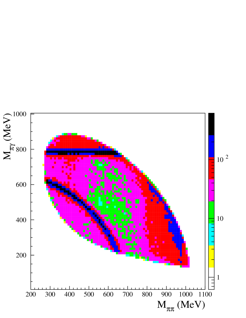
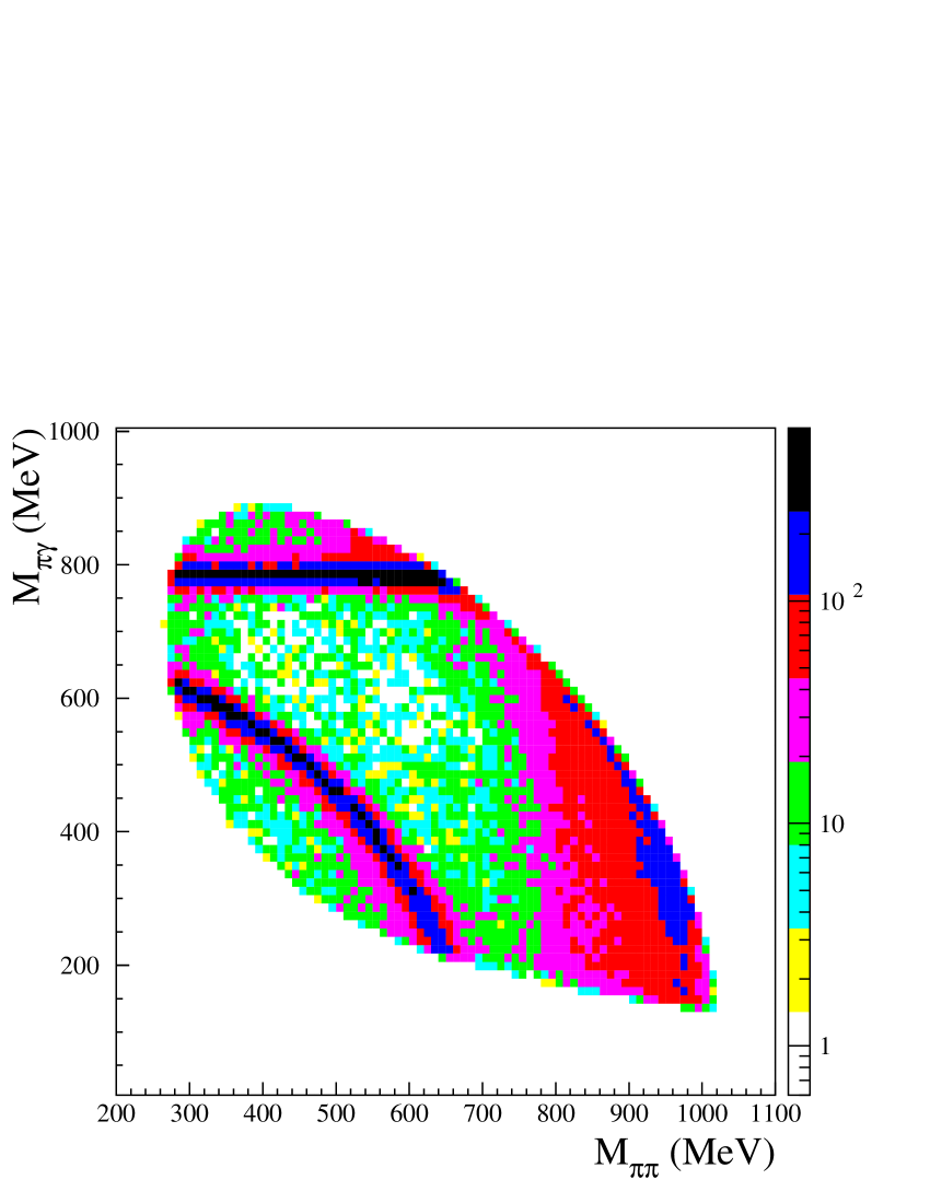
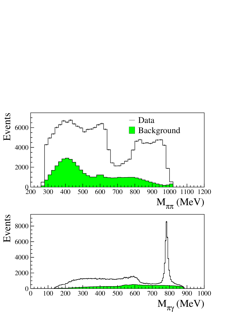
The two kinematic variables chosen for the construction of the Dalitz plot are the invariant masses of the two $\pi^{0}$’s, $M_{\pi\pi}$, and of the two possible $\mbox{$\pi^{0}$}\gamma$ combinations, $M_{\pi\gamma}$. We have therefore two entries per event. The binning choice, driven by the mass resolutions obtained by Monte Carlo for the signal, is 10 MeV for $M_{\pi\pi}$ and 12.5 MeV for $M_{\pi\gamma}$. The data density is shown in Fig. 6 before and after background subtraction. The two projections are shown in Fig. 7. After background subtraction the number of events in the Dalitz plot is $128,529\pm 659$.

Figure 6: Dalitz plot in logarithmic scale before (left) and after (right) background subtraction. The two bands in the region $\mbox{$M_{\pi\pi}$}<700$ MeV are due to $\mbox{$e^{+}$}\mbox{$e^{-}$}\to\omega\mbox{$\pi^{0}$}$ events.

Figure 7: Dalitz plot projections in $M_{\pi\pi}$ (top) and $M_{\pi\gamma}$ (bottom) variables before background subtraction.

The analysis efficiency as a function of $M_{\pi\pi}$ and $M_{\pi\gamma}$ is evaluated by Monte Carlo, with corrections based on data control samples. In Fig. 8 the dependence of the selection efficiency on $M_{\pi\pi}$ and $M_{\pi\gamma}$ is shown for the $S\gamma$ and $\omega\pi$ final states. Both processes exhibit a rather flat dependence on the Dalitz plot variables. The different shape is related to their angular distribution and to their different probability of producing photons from initial state radiation (ISR). The main source of data-MC differences is due to the photon detection efficiency, which is measured as a function of $E_{\gamma}$ with $\phi\to\pi^{+}\pi^{-}\pi^{0}$ control samples and applied, as a correction, to the Monte Carlo. The MC trigger, cosmic ray veto and event classification filter efficiencies are checked using prescaled data samples. The overall correction factor, $R_{\rm sel}=1.022\pm 0.004$, is applied to the MC analysis efficiency.

Figure 8: Analysis efficiency for $S\gamma$ (empty triangles) and $\omega\pi$ (black dots) MC events as a function of $M_{\pi\pi}$ (top) and $M_{\pi\gamma}$ (bottom).

4 Fit to the Dalitz plot

4.1 Fitting method

The double differential $\mbox{$\pi^{0}$}\mbox{$\pi^{0}$}\gamma$ cross section is written as the sum of the scalar term, the VMD contribution and of their relative interference as follows:

$$\frac{d\sigma}{d\mbox{$M_{\pi\pi}$}dM_{\pi\gamma}}=$$ (1)

$$\ \ \ \frac{d\sigma^{S}}{d\mbox{$M_{\pi\pi}$}dM_{\pi\gamma}}+\frac{d\sigma^{V}}{d\mbox{$M_{\pi\pi}$}dM_{\pi\gamma}}\pm\frac{d\sigma^{I}}{d\mbox{$M_{\pi\pi}$}dM_{\pi\gamma}}.$$

The suffixes $S$ and $V$ stand for $S\gamma$ and VMD terms while $I$ represents the interference. To fit the Dalitz plot data density, the theory is folded with the reconstruction efficiencies of the two processes and with the probability for an event to migrate from a Dalitz plot bin to another one. The expected number of events for a given reconstructed $M_{\pi\pi}$, $M_{\pi\gamma}$ bin $i$, $N^{\rm exp}_{i}$, is then computed from the total integrated luminosity, $L_{\rm int}$, as follows:

$$N^{\rm exp}_{i}=\mbox{$L_{\rm int}$}\times$$ (2)

$$\ \ \ \ \sum_{j}\,(f^{V}_{j}\ A^{V}_{i,j}\ \varepsilon^{V}_{j}+f^{S}_{j}\ A^{S}_{i,j}\ \varepsilon^{S}_{j}+f^{I}_{j}\ A^{V}_{i,j}\ \varepsilon^{V}_{j})\,.$$

where $f_{j}$ is the integration of the differential cross section evaluated in the $j^{\rm th}$ bin, including the effect of the ISR. For each bin, $\varepsilon_{j}$ is the analysis efficiency while $A_{i,j}$ is the smearing matrix, representing the probability for the signal event to migrate from the $j^{\rm th}$ to the $i^{\rm th}$ bin, either due to resolution or to a wrong reconstruction of the event. This matrix has been evaluated by Monte Carlo: about 85% of the events are on the diagonal or close to it, within $\pm 1$ bin. The remaining 15% is mostly due to events where photons are incorrectly paired to $\pi^{0}$’s. A dedicated data-MC comparison has been performed to calibrate the fraction of good/bad pairing. The difference between the two lowest values of pseudo-$\chi^{2}$ used to pair photons, $\Delta\chi^{2}_{\rm pair}$, is fit with a superposition of the two templates obtained for MC events with good and bad photon pairing (Fig. 9). A data-MC difference of $1.08\pm 0.02$ is found and is taken into account in evaluating the systematic error.

Figure 9: Top: Monte Carlo $\Delta\chi^{2}_{\rm pair}$ shapes for events with correct and wrong photon pairing. These two templates are used to fit the $\Delta\chi^{2}_{\rm pair}$ data distribution (bottom). A better data-MC agreement is obtained after the fit.

4.2 Theoretical models

A more explicit formulation of the differential cross section (1) is reported in Appendix A. Concerning the scalar term, we use two different approaches for the description of the amplitude: the Kaon Loop model (KL) KaonLoop ; KaonLoopSigma ; KaonLoopNew , where the scalar is coupled to the $\phi$ through a charged kaon loop, and another formulation called No Structure (NS) NoStructure , where the $\phi S\gamma$ coupling is point-like and the scalar is described as a Breit-Wigner with a mass dependent width added to a complex function, to allow an appropriate behaviour of the resulting shape at low masses.

4.2.1 Kaon Loop model

As scalar term of the Kaon Loop model we use the one described in Ref. KaonLoopNew , where the amplitude of the signal

$$M_{S\gamma}=e^{i\delta_{B}}g(M_{\pi\pi})\,\left(\sum_{S,S^{\prime}}g_{SK^{+}K^{-}}\,G^{-1}_{SS^{\prime}}\,g_{S^{\prime}\pi^{0}\pi^{0}}\right),$$ (3)

implies the mixing of two scalar states, namely the $f_{0}$(980) and the $\sigma(600)$, represented by the $G_{SS^{\prime}}$ matrix. The $g(M_{\pi\pi})$ function describes the kaon loop and $g_{S\pi\pi/KK}$ are the couplings of the scalars to the $\pi\pi/\mbox{$K\overline{K}$}$ mesons. Differently from the past, where the phase $\delta_{B}$ took into account only the elastic scattering due to $\pi\pi$, in this new formulation the scattering due to $K\overline{K}$ is also considered.

Using this theoretical framework, our $\pi^{0}$$\pi^{0}$ mass spectrum obtained from 2000 data PLBf0n2002 , has been fit by the authors of Ref. KaonLoopNew together with $\pi\pi$ scattering data ScattData1 ; ScattData2 ; ScattData3 ; ScattData4 ; ScattData5 , providing ten sets of parameters which are able to describe both data samples. For all of them, the $\sigma(600)$ coupling to $K\overline{K}$ is small with respect to the one of $\pi\pi$ and its mass lies in the 500–700 MeV range. This means a very broad meson width, between 240 and 490 MeV. All the odd (even) variants have a positive (negative) $g_{\sigma\pi^{+}\pi^{-}}/g_{f_{0}K^{+}K^{-}}$ ratio.

When fitting the Dalitz plot of our new data set, we can not leave all $f_{0}(980)$ and $\sigma(600)$ parameters free, as the description of the elastic background and the couplings and masses of the $\sigma(600)$ meson are closely related. We therefore proceed by using as free parameters only the VMD ones and the mass and the coupling to $\pi^{+}$$\pi^{-}$ and $K\overline{K}$ of the $f_{0}$(980), using the isospin relations $g_{f_{0}\pi^{0}\pi^{0}}=1/\sqrt{2}g_{f_{0}\pi^{+}\pi^{-}}=1/\sqrt{3}g_{f_{0}\pi\pi}$ and $g_{f_{0}KK}=g_{f_{0}K^{+}K^{-}}=g_{f_{0}K^{0}\overline{K}^{0}}$. For the $\sigma(600)$ and the elastic $\pi\pi$ and $K\overline{K}$ scattering we use the values of Ref. KaonLoopNew by repeating the fit for all the ten available sets of parameters. We obtain $P(\chi^{2})$ ranging from $10^{-5}$ to 0.145; only the six results with $P(\chi^{2})>1\%$ are kept for the present discussion.

Furthermore, the case of a single scalar contribution, the $f_{0}$(980), in the Kaon Loop description has also been tried by using the old KL parametrization KaonLoopSigma . The resulting $P(\chi^{2})$ of the fit is not acceptable, showing the need of introducing the $\sigma(600)$.

4.2.2 No Structure model

In the NS description, the amplitude of the scalar term is proportional to a scalar form factor, $F_{0}^{\rm scal}$, which is derived by assuming a direct coupling of the $\phi$ to the $f_{0}(980)$, $g_{\phi f_{0}\gamma}$, and a subsequent coupling of the $f_{0}(980)$ to the $\pi\pi$ pair, $g_{f_{0}\pi\pi}$. In the same form factor the possible non-resonant continuum background is also added as a series expansion in $M_{\pi\pi}$ as follows:

$$F_{0}^{\rm scal} = \frac{g_{f_{0}\pi^{0}\pi^{0}}\,g_{\phi f_{0}\gamma}}{M_{\pi\pi}^{2}-M_{f_{0}}^{2}+i\,M_{\pi\pi}\Gamma_{f_{0}}(M_{\pi\pi})}+$$

$$\frac{a_{0}}{M_{\phi}^{2}}e^{ib_{0}\frac{v_{\pi}(M_{\pi\pi})}{M_{\phi}}}+\frac{a_{1}}{M_{\phi}^{4}}e^{ib_{1}\frac{v_{\pi}(M_{\pi\pi})}{M_{\phi}}}(M_{\pi\pi}^{2}-M_{f_{0}}^{2}),$$

where, in the most general case, the background parameters are complex numbers and $v_{\pi}(M_{\pi\pi})$ is proportional to pion momentum in the scalar rest frame, $v_{\pi}=\sqrt{M_{\pi\pi}^{2}/4-M_{\pi}^{2}}$. The propagator for the $f_{0}$(980) resonance is described by a simple Breit-Wigner shape corrected by the Flattè condition on the $\pi\pi$ and $KK$ thresholds, i.e.:

$$\Gamma_{f_{0}}(M_{\pi\pi}) = g_{f_{0}\pi\pi}^{2}\frac{v_{\pi}(M_{\pi\pi})}{8\pi M_{\pi\pi}^{2}}+$$

$$g_{f_{0}KK}^{2}\frac{v_{K^{\pm}}(M_{\pi\pi})+v_{K^{0}}(M_{\pi\pi})}{8\pi M_{\pi\pi}^{2}},$$

where $v_{\pi,K,K^{0}}$ are complex numbers with an analytical continuation under threshold and the coupling to $\pi\pi$ and $K\overline{K}$ have the same meaning as in the KL description. In this model the fit parameters are $M\mbox{${}_{f\!_{0}}$}$, $g_{f_{0}\pi^{+}\pi^{-}}$, $g_{f_{0}KK}$, $g_{\phi f_{0}\gamma}$ and the background parameters $a_{0}$, $a_{1}$ and $b_{1}$. The $b_{0}$ phase is fully determined as a function of the other parameters.

4.3 Fit Systematics

There are different sources of systematics affecting this analysis which can give rise to variations of the fit results. We describe here the most important ones. For each of them, the fit is repeated after changing the relevant quantity within its range of uncertainty. In Tabs. 2, 3 we show the corresponding percentage variation of the interesting free parameters for the KL, NS model respectively.

Table 2: Fractional systematic error on fit parameters for the KL scalar term. Only variations above 0.1% are reported.

Parameter	$M\!\mbox{${}_{f\!_{0}}$}$	$g_{\!f_{0}K^{+}K^{-}}$	$g_{\!f_{0}\pi^{+}\pi^{-}}$
Source	Fractional systematic error
Normalization	—	$\pm 1.6\%$	$\pm 0.7\%$
Beam energy	—	$+2.4\%$	$-1.4\%$
Photon efficiency	—	$-2.1\%$	$+1.4\%$
$\chi^{2}$ cut	—	$-0.8\%$	—
Smearing matrix	$-0.1\%$	—	$+1.4\%$
Interference	—	$-1.1\%$	$+0.7\%$
Background	$+0.1\%$	$+4.0\%$	$-3.5\%$

Table 3: Fractional systematic error on fit parameters for the NS scalar term. Only variations above 0.1% are reported.

Parameter	$M\!\mbox{${}_{f\!_{0}}$}$	$g_{\!f_{0}K^{+}K^{-}}$	$g_{\!f_{0}\pi^{+}\pi^{-}}$	$g_{\phi f_{0}\gamma}$	$a_{0}$	$a_{1}$	$b_{1}$
Source	Fractional systematic error
Normalization	$\pm 0.1\%$	${}^{+155\%}_{-\phantom{1}50\%}$	${}^{+6.9\%}_{-1.5\%}$	${}^{+11.9\%}_{-\phantom{1}1.9\%}$	${}^{+34.4\%}_{-\phantom{3}5.5\%}$	${}^{+122\%}_{-\phantom{1}16\%}$	${}^{+57.3\%}_{-16.7\%}$
Beam energy	$-0.2\%$	$+82.5\%$	$+0.8\%$	$+1.9\%$	—	—	$-\phantom{2}3.3\%$
Photon efficiency	$+0.2\%$	$-72.5\%$	$+3.1\%$	$+3.4\%$	$+17.9\%$	$+49.6\%$	$+29.3\%$
$\chi^{2}$ cut	$-0.2\%$	$+57.5\%$	$+2.3\%$	$-2.3\%$	$+\phantom{1}1.7\%$	$+17.6\%$	$+20.0\%$
Smearing matrix	$-0.2\%$	$-\phantom{7}7.5\%$	$-2.3\%$	$-3.1\%$	$-10.0\%$	$-26.0\%$	$-28.0\%$
Interference	—	$+82.5\%$	$+3.1\%$	$+5.4\%$	$+18.1\%$	$+69.5\%$	$+46.0\%$
Background	$-0.4\%$	$+92.5\%$	—	$-2.3\%$	$-8.4\%$	$-8.4\%$	$+\phantom{2}4.0\%$

1. Normalization
   The first effect considered is the normalization scale of the fit estimate on the event counting. When evaluating $N^{\rm exp}_{i}$, two experimentally determined constants are used: the integrated luminosity and the value of the $\phi$ leptonic width. The luminosity is known with a total error of 0.6% EPJ_Lumi while the leptonic width has been measured by KLOE with a 1.7% uncertainty PLB_Gee . The fit has been repeated by changing the value of both quantities of $\pm 1\sigma$.

2. Beam energy scale
   The beam energy scale also affects the fit due to the explicit $\sqrt{s}$ dependence of the theoretical function. Bhabha scattering events allow a relative calibration of the energy scale with a precision of 30 keV each 100 nb^-1 of integrated luminosity. As mentioned in the introduction, an absolute calibration of 150 keV has been applied to match the measured value of $M_{\phi}$. The fit to the Dalitz plot has been repeated without applying this correction.

3. Photon efficiency
   The data-MC correction of the cluster efficiency curve modifies the shape of the Dalitz plot. A different parametrization of the cluster efficiency curves in the Monte Carlo KN_Ks2pi_2006 has been used to evaluate anew the smearing matrix, the analysis efficiency and the background contribution. The fit has been repeated in these conditions.

4. $\chi^{2}$ cut
   To test the systematic contribution of the chosen $\chi^{2}$ cut, we have repeated the whole analysis hardening the $\chi^{2}_{\rm Fit2}/{\rm N_{dof}}$ cut from 5 to 3. In this way the event counting is improved due to the large reduction of background while the analysis efficiency is not as flat as before along the Dalitz plot due to the ISR tails.

5. Smearing matrix
   From the measured quantity of wrong photon pairing (Sec. 4.1), the fraction of off-diagonal events in the smearing matrix has been increased by 8%.

6. Interference
   In the standard fit function, the radiative corrections, the analysis efficiency and the smearing matrix used in the interference term are obtained from an MC sample of $\omega\pi$ events. The fit is repeated by using the corresponding quantities estimated with $S\gamma$ events.

7. Background
   The scale factors $\alpha_{1}$, obtained when fitting the background-enriched distributions, are applied to the residual background contamination.

As shown in Tabs. 2, 3, the KL fit provides stable results when the systematic changes are applied. On the other hand, the NS fit shows very large parameter variations due to the presence of the continuum background term.

4.4 Fit results

4.4.1 Kaon Loop model

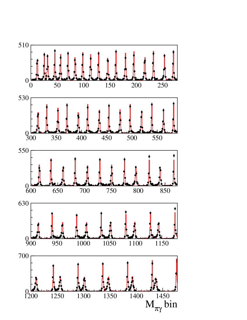
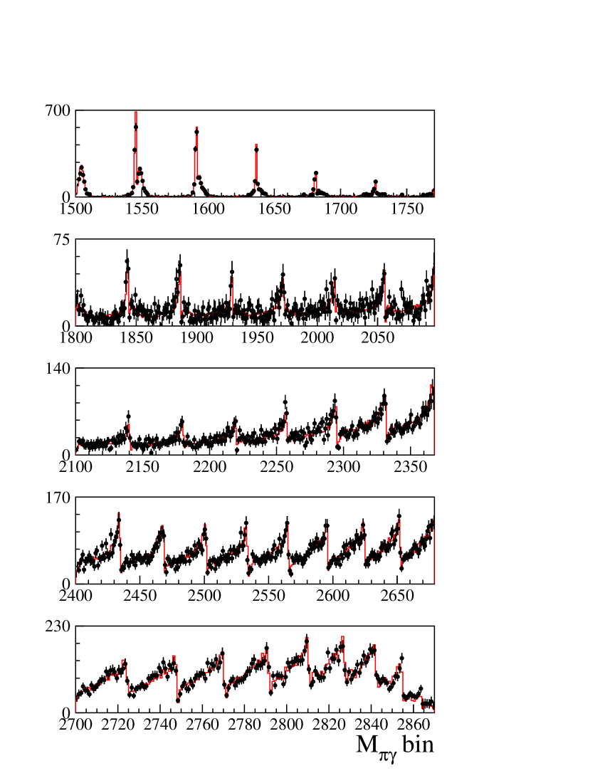
The Kaon Loop fit results are listed in Tabs. 4, 5 for the six accepted variants. In Fig. 10 the distributions of the data points for all slices of the Dalitz plot with the superimposed fit function of the variant with the best $P(\chi^{2})$ is shown. Here the $M_{\pi\gamma}$ vs $M_{\pi\pi}$ histogram is sliced in $M_{\pi\pi}$ and for each slice the $M_{\pi\gamma}$ projection of the allowed phase-space region is plotted, one after the other. To understand the relative importance of the different fitting terms, their contributions are shown in Fig. 12.left. As expected, the VMD ($S\gamma$) term is dominating in the region below (above) 700 MeV. The interference term is concentrated around 600 MeV. As a fit result, we use the central value and the errors from the best fit, adding the systematic error discussed in the previous section and an extra error associated with the theoretical model. This last error is evaluated as the maximum variation between the central value obtained by the best fit ($P(\chi^{2})=0.145$) and the other five accepted fits.

Figure 10: Fit result for Kaon Loop model. Black dots are data while the solid line represents the KL resulting shape.

Table 4: Fit results for the scalar term in the Kaon Loop model. Different rows are obtained for the accepted sets of parameters from Ref. KaonLoopNew .

Fit	$M\!\mbox{${}_{f\!_{0}}$}$ (MeV)	$g_{\!f_{0}K^{+}K^{-}}$ (GeV)	$g_{\!f_{0}\pi^{+}\pi^{-}}$ (GeV)	$M_{\sigma},\Gamma\!_{\sigma}$ (MeV)	$\chi^{2}$/Ndof	$P(\chi^{2})$
K1	$976.8\pm 0.3$	$3.76\pm 0.04$	$-1.43\pm 0.01$	$462\,,286$	2754/2676	$0.145$
K2	$986.2\pm 0.3$	$3.87\pm 0.08$	$-2.03\pm 0.02$	$485\,,240$	2792/2676	$0.058$
K3	$985.2\pm 0.2$	$4.92\pm 0.06$	$-1.92\pm 0.01$	$472\,,320$	2809/2676	$0.036$
K4	$982.3\pm 0.4$	$4.02\pm 0.06$	$-1.76\pm 0.02$	$415\,,260$	2787/2676	$0.066$
K5	$983.3\pm 0.2$	$3.75\pm 0.02$	$-1.40\pm 0.01$	$529\,,366$	2823/2676	$0.024$
K6	$986.9\pm 0.1$	$3.28\pm 0.05$	$-1.90\pm 0.01$	$566\,,264$	2799/2676	$0.048$

Table 5: Fit results for the VMD parametrization. The first six rows are obtained in the KL approach for the accepted sets of parameters from Ref. KaonLoopNew while the last line is the result of the NS fit.

Fit	$\alpha_{\rho\pi}$	$C_{\omega\pi}$ (GeV-2)	$\phi_{\omega\pi}$	$C_{\rho\pi}$ (GeV-2)	$\phi_{\rho\pi}$	$\delta_{b_{\rho}}$ (∘)	$M_{\omega}$ (MeV)
K1	$0.58\pm 0.11$	$0.850\pm 0.010$	$0.46\pm 0.13$	$0.260\pm 0.185$	$3.11\pm 3.12$	$33.0\pm 9.7$	$782.52\pm 0.29$
K2	$0.68\pm 0.03$	$0.832\pm 0.003$	$0.30\pm 0.05$	$0.061\pm 0.211$	$3.14\pm 3.08$	$23.6\pm 4.1$	$782.20\pm 0.11$
K3	$0.66\pm 0.17$	$0.836\pm 0.004$	$0.33\pm 0.08$	$0.084\pm 0.056$	$3.14\pm 3.14$	$25.2\pm 6.2$	$782.26\pm 0.28$
K4	$0.64\pm 0.05$	$0.836\pm 0.002$	$0.38\pm 0.06$	$0.061\pm 0.005$	$3.14\pm 0.04$	$31.3\pm 2.4$	$782.28\pm 0.14$
K5	$0.62\pm 0.01$	$0.838\pm 0.006$	$0.27\pm 0.04$	$0.298\pm 0.126$	$3.13\pm 0.07$	$10.4\pm 6.5$	$782.41\pm 0.07$
K6	$0.58\pm 0.04$	$0.843\pm 0.004$	$0.30\pm 0.06$	$0.061\pm 0.003$	$3.14\pm 0.01$	$33.7\pm 4.8$	$782.48\pm 0.13$
NS	$1.43\pm 0.04$	$0.953\pm 0.003$	$0.00\pm 0.01$	$0.270\pm 0.039$	$3.11\pm 0.14$	$73.1\pm 1.6$	$781.80\pm 0.11$

The extracted parameters are:

$$M\!\mbox{${}_{f\!_{0}}$}=(976.8\pm 0.3_{\rm\,fit}\,^{+0.9}{}_{-0.6}\,{}_{\rm syst}+10.1_{\rm\,mod})\ {\rm MeV}$$

$$g_{\!f_{0}K^{+}K^{-}}=(3.76\pm 0.04_{\rm\,fit}\,^{+0.15}{}_{-0.08}\,{}_{\rm syst}\,^{+1.16}{}_{-0.48}\,{}_{\rm mod})\ {\rm GeV}$$

$$g_{\!f_{0}\pi^{+}\pi^{-}}=(-1.43\pm 0.01_{\rm\,fit}\,^{+0.01}{}_{-0.06}\,{}_{\rm\,syst}\,^{+0.03}{}_{-0.60}\,{}_{\rm mod})\ {\rm GeV}$$

$$R\mbox{${}_{f\!_{0}}$}=\frac{g^{2}_{\!f_{0}K^{+}K^{-}}}{g^{2}_{\!f_{0}\pi^{+}\pi^{-}}}=6.9\pm 0.1_{\rm\,fit}\,^{+0.2}{}_{-0.1}\,{}_{\rm syst}\,^{+0.3}{}_{-3.9}\,{}_{\rm mod}$$

$$g_{\phi f_{0}\gamma}=(2.78\,^{+0.02}_{-0.05}\,{}_{\rm fit}\,^{+0.13}{}_{-0.05}\,{}_{\rm syst}+1.31_{\rm\,mod})\ {\rm GeV}^{-1}$$

The first three quantities are the parameters directly extracted from the fit while the other two are derived. The $g_{\phi f_{0}\gamma}$ coupling is obtained using the formula

$$g_{\phi f_{0}\gamma}=\sqrt{\frac{3}{\alpha}\left(\frac{2M_{\phi}}{M_{\phi}^{2}-M_{f_{0}}^{2}}\right)^{3}\Gamma_{\phi}\,3\,\mbox{BR}(\phi\to S\gamma\to\pi^{0}\pi^{0}\gamma)}.$$

4.4.2 No Structure model

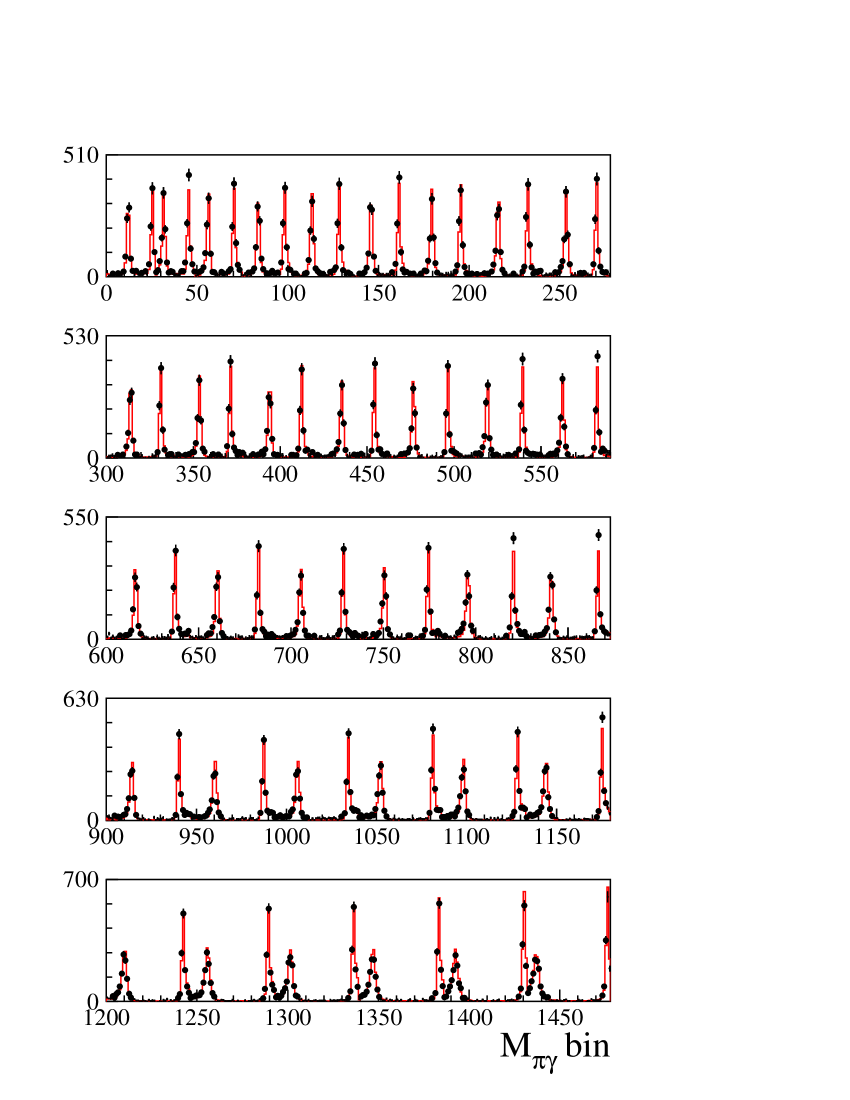
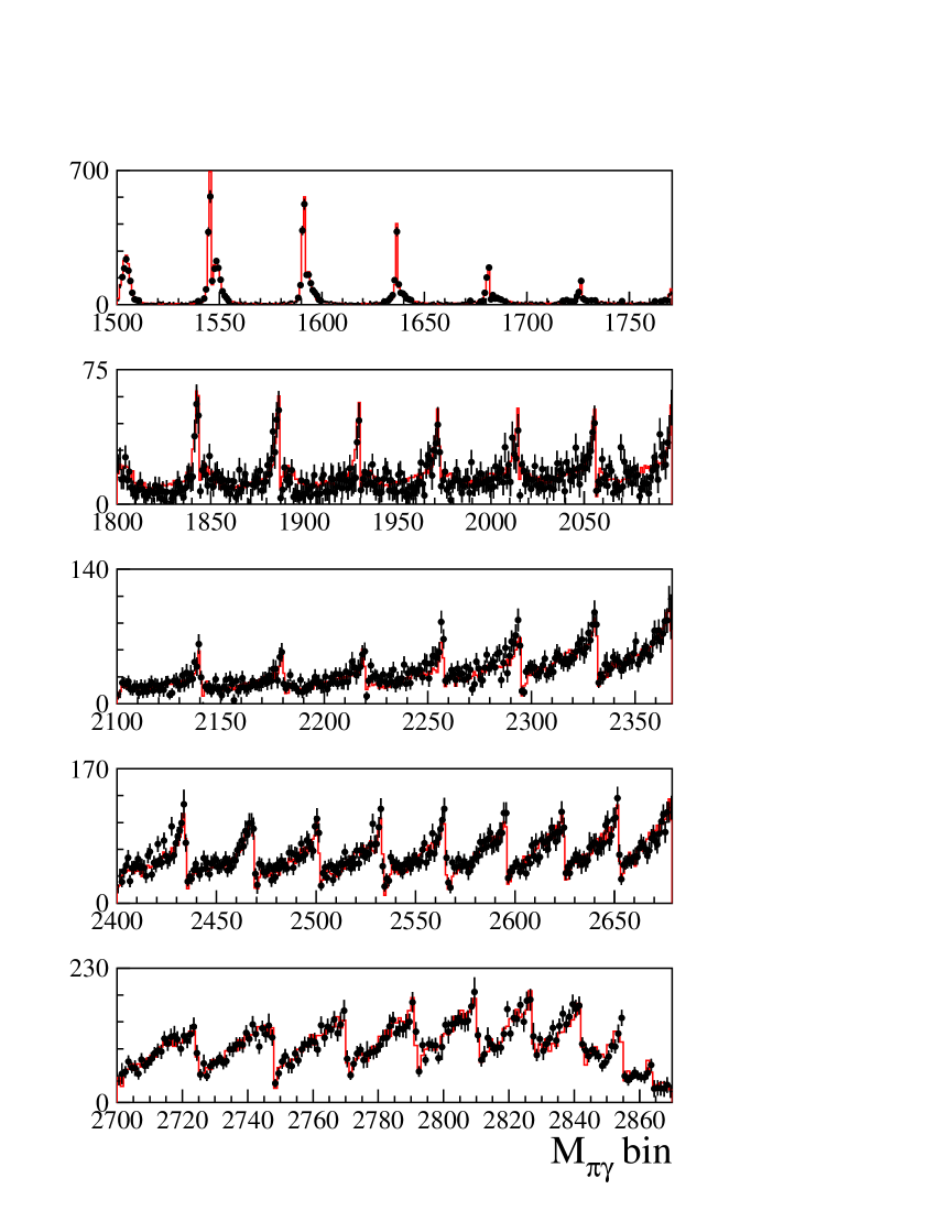
In the No Structure model the resonant term is described with a single narrow meson pole, the $f_{0}$(980), added to a continuum $\phi\to\mbox{$\pi^{0}$}\mbox{$\pi^{0}$}\gamma$ background described by the three free parameters $a_{0}$, $a_{1}$ and $b_{1}$. The fit quality, having a $P(\chi^{2})=0.042$, is a little worse than the best KL result but still acceptable (see Fig. 11). The different components of the fit are shown in Fig. 12.right. Again, for $\mbox{$M_{\pi\pi}$}>700$ MeV the scalar contribution is clearly dominant. However, contrary to the KL case, the interference term gets negative in this region, so that the scalar term is slightly increased. The VMD fit parameters are listed in Tab. 5 while for the scalar term we have:

$$M\!\mbox{${}_{f\!_{0}}$}=(984.7\pm 0.4_{\rm\,fit}\,^{+2.4}{}_{-3.7}\,{}_{\rm\,syst})\ {\rm MeV}$$

$$g_{\!f_{0}K^{+}K^{-}}=(0.40\pm 0.04_{\rm\,fit}\,^{+0.62}{}_{-0.29}\,{}_{\rm\,syst})\ {\rm GeV}$$

$$g_{\!f_{0}\pi^{+}\pi^{-}}=(1.31\pm 0.01_{\rm\,fit}\,^{+0.09}{}_{-0.03}\,{}_{\rm\,syst})\ {\rm GeV}$$

$$R\mbox{${}_{f\!_{0}}$}=\frac{g^{2}_{\!f_{0}K^{+}K^{-}}}{g^{2}_{\!f_{0}\pi^{+}\pi^{-}}}=0.09\pm 0.02_{\rm\,fit}\,^{+0.44}{}_{-0.08}\,{}_{\rm\,syst}$$

$$g_{\phi f_{0}\gamma}=(2.61\pm 0.02_{\rm\,fit}\,^{+0.31}{}_{-0.08}\,{}_{\rm\,syst})\ {\rm GeV^{-1}}$$

$$a_{0}=\hphantom{-}4.19\pm 0.01_{\rm\,fit}\,^{+1.44}{}_{-0.42}\,{}_{\rm syst}$$

$$a_{1}=\hphantom{-}1.31\pm 0.01_{\rm\,fit}\,^{+1.60}{}_{-0.34}\,{}_{\rm syst}$$

$$b_{1}=-1.50\pm 0.02_{\rm\,fit}\,^{+0.86}{}_{-0.42}\,{}_{\rm\,syst}$$

Here the only parameter that is not directly extracted from the fit is R${}_{f\!_{0}}$.

Figure 11: Fit result for No Structure model. Black dots are data while the solid line represents the NS resulting shape.

Figure 12: Resulting $\mbox{$\pi^{0}$}\mbox{$\pi^{0}$}\gamma$ contributions for Kaon Loop (left) and No Structure (right) models.

4.4.3 KL, NS combined results

In Fig. 13 the comparison of the scalar contributions obtained from the six KL fit results shows stable resulting shapes. On the contrary, comparing the KL and NS curves there are differences at a level of few % (Fig. 13), mainly due to the interference term. In the same figure, the result of the fit obtained with the old $f_{0}$(980)+$\sigma(600)$ parametrization on 2000 data PLBf0n2002 is shown. The small bump below 500 MeV is now described by the $S\gamma$-VMD interference. By integrating the KL, NS distributions and normalizing to the $\phi$ production cross section, an effective BR for the $\phi\to S\gamma\to\mbox{$\pi^{0}$}\mbox{$\pi^{0}$}\gamma$ process is extracted:

$$\mbox{BR}(\phi\to S\gamma\to\mbox{$\pi^{0}$}\mbox{$\pi^{0}$}\gamma)=$$

$$\ \ \ \ \ \ \ (1.07\,^{+0.01}_{-0.03}\,{}_{\rm fit}\,^{+0.04}{}_{-0.02}\,{}_{\rm syst}\;^{+0.05}{}_{-0.06}\;{}_{\rm mod})\times 10^{-4}$$

The central value is given by the KL model with the best $P(\chi^{2})$, the fit error has been evaluated as the maximum excursion obtained when varying the fit errors by $\pm 1\sigma$ and the model error corresponds to the maximum variation of the central value with respect to the other five accepted fit results of the KL model and to the NS description.

Figure 13: $M_{\pi\pi}$ distribution of the $\phi\to S\gamma\to\mbox{$\pi^{0}$}\mbox{$\pi^{0}$}\gamma$ process obtained from the fit. Top: comparison between the six accepted results of the KL model. Bottom: comparison between the best KL fit, the NS resulting shape and the previous KLOE measurement PLBf0n2002 .

4.4.4 Extrapolation to other $\sqrt{s}$ points

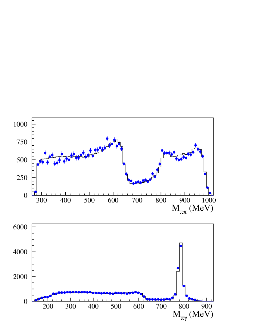
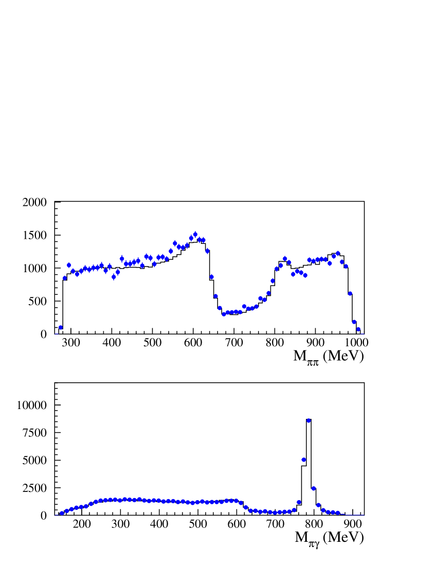
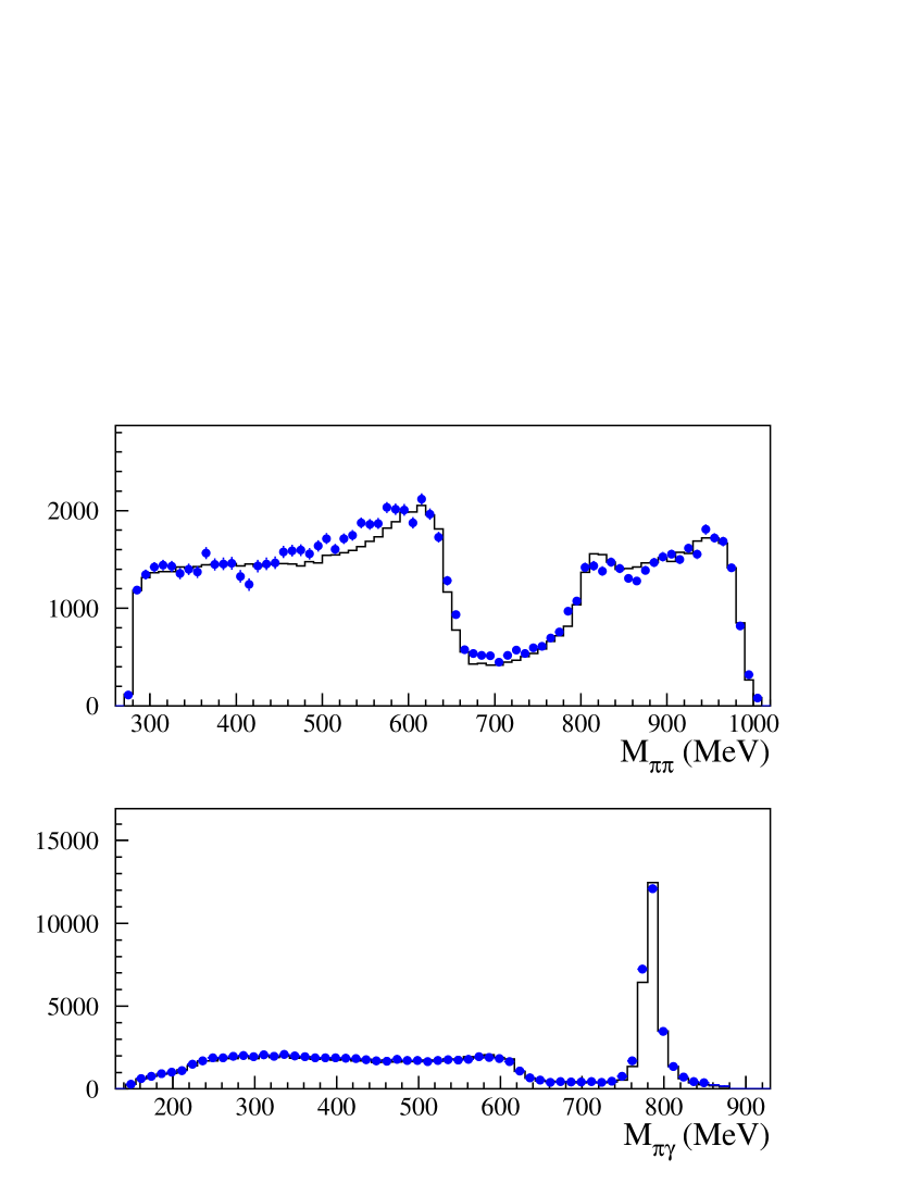
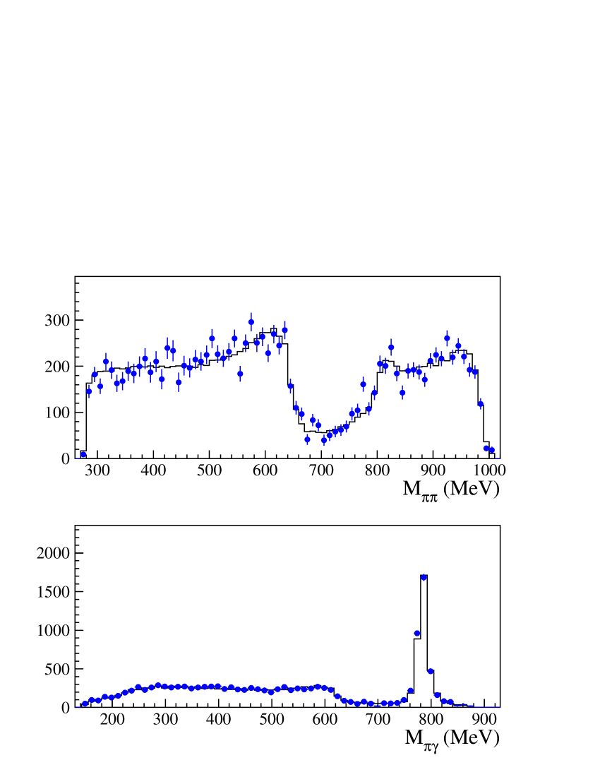
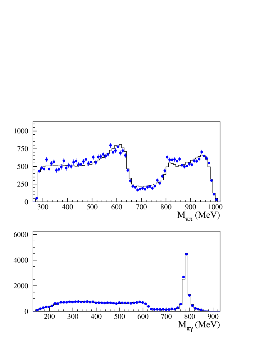
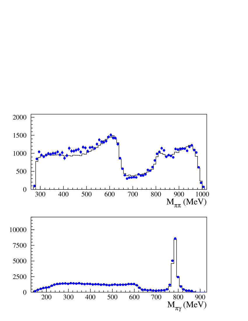
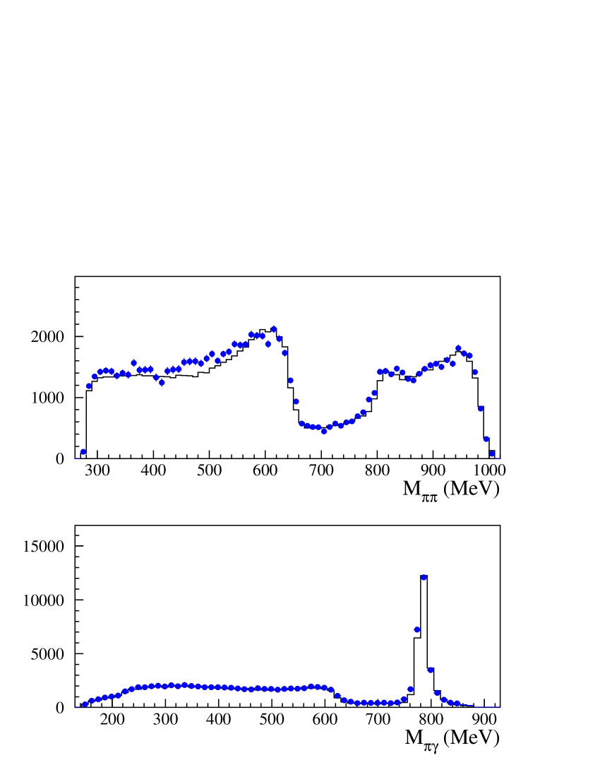
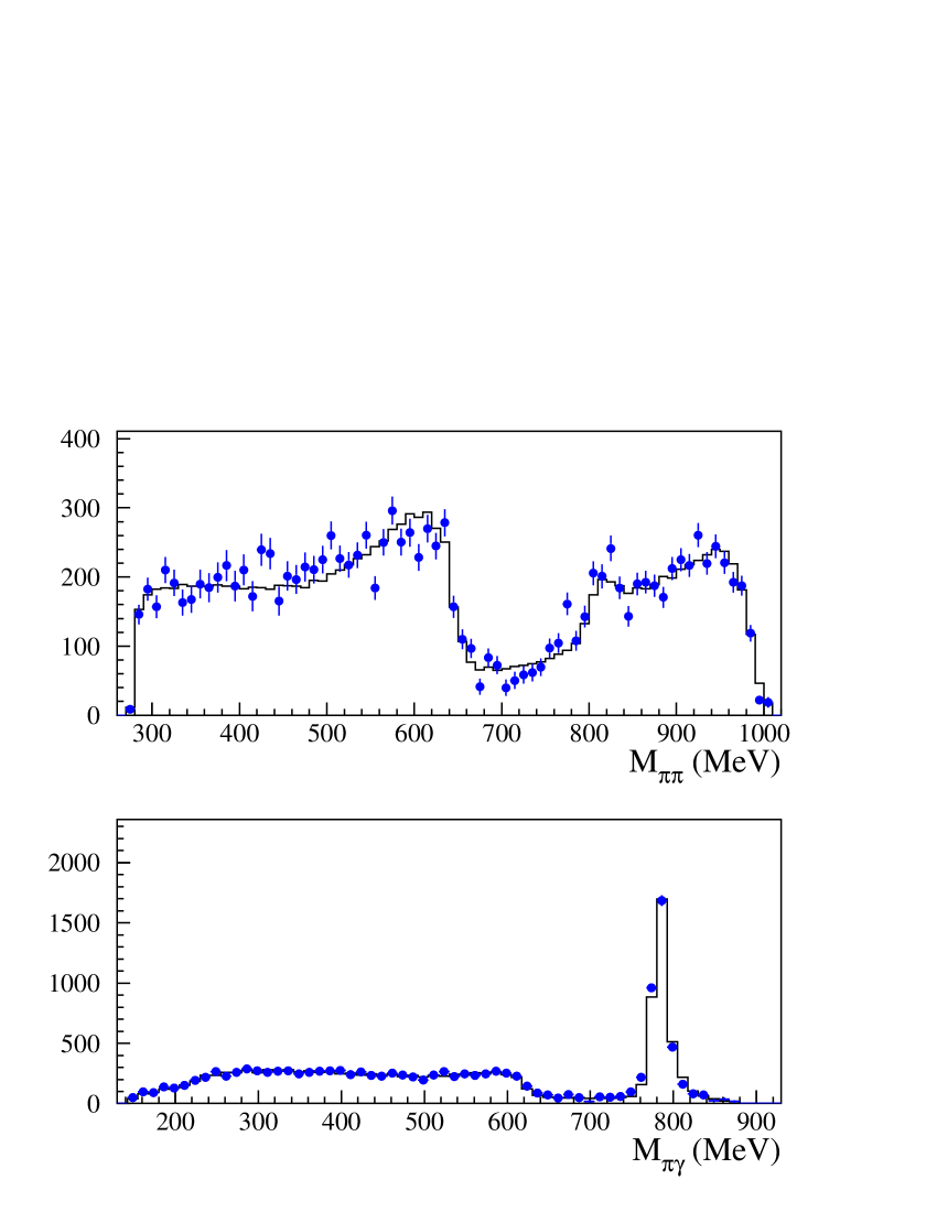
As a last check, we extrapolate both KL and NS fit results to the four closest $\sqrt{s}$ points: 1019.55 MeV (42 pb^-1), 1019.65 MeV (77 pb^-1), 1019.85 MeV (100 pb^-1) and 1019.95 MeV (15 pb^-1), scaling for the integrated luminosity. As shown in Figs. 14 and 15, a good agreement is obtained in all the $M_{\pi\pi}$ and $M_{\pi\gamma}$ distributions.

Figure 14: Dalitz plot projections for runs with different $\sqrt{s}$: 1019.55 MeV (top-left), 1019.65 MeV (top-right), 1019.85 MeV (bottom-left) and 1019.95 MeV (bottom-right). Data are reported in dots while the solid line represents the expected shape extrapolated from fit K1 of the Kaon Loop model.

Figure 15: Dalitz plot projections for runs with different $\sqrt{s}$: 1019.55 MeV (top-left), 1019.65 MeV (top-right), 1019.85 MeV (bottom-left) and 1019.95 MeV (bottom-right). Data are reported in dots while the solid line represents the expected shape extrapolated from NS fit.

4.5 Comparison with $\mbox{$\pi^{+}$}\mbox{$\pi^{-}$}\gamma$ final state

In principle it is possible to compare these results with those obtained by KLOE on the charged channel $\mbox{$e^{+}$}\mbox{$e^{-}$}\to\mbox{$\pi^{+}$}\mbox{$\pi^{-}$}\gamma$ PLBf0c2005 . However in this case the non resonant background (dominated by the $\rho$ radiative tail) is much more important, so that the extraction of the $f_{0}$(980) signal is more difficult and there is a reduced sensitivity to the presence of the $\sigma(600)$.

The results of the fit with the KL or NS model yield consistent values for the $f_{0}$(980) mass and for the branching ratio while large discrepancies are observed on the differential cross section, especially for the NS model.

More precisely, by scaling by a factor two the extracted cross-section for the $\pi^{0}\pi^{0}\gamma$ case, we estimate BR($\phi\to S\gamma\to\mbox{$\pi^{+}$}\mbox{$\pi^{-}$}\gamma)=(2.14\pm 0.14)\times 10^{-4}$, to be compared to the values from $\mbox{$\pi^{+}$}\mbox{$\pi^{-}$}\gamma$ data: $(2.1\pm 0.4)\times 10^{-4}$ (KL model) and $(2.4\pm 0.5)\times 10^{-4}$ (NS model).

For the KL model, a still acceptable agreement on the $f_{0}(980)$ coupling constants is observed, although the $\sigma(600)$ is not needed in the $\mbox{$\pi^{+}$}\mbox{$\pi^{-}$}\gamma$ case. This is mainly due to the improved parametrization of the KL which had not been used for the charged case. For the NS model instead large differences are found on all couplings.

5 Conclusions

The analysis of the $\mbox{$\pi^{0}$}\mbox{$\pi^{0}$}\gamma$ final state presented here treats equally the two main production mechanisms, the VMD and $S\gamma$ processes. The high statistics (145 pb^-1 in a single $\sqrt{s}$ bin) allowed us to fit with two different theoretical models the Dalitz plot distribution. In the Kaon Loop model, the two low mass scalars $f_{0}(980)$ and $\sigma(600)$ are required to adequately fit the data. In the case of the No Structure model, we instead find an acceptable fit with the $f_{0}(980)$ meson alone. In the latter formulation the low mass $M_{\pi\pi}$ behaviour is described by the three free parameters $a_{0}$, $a_{1}$ and $b_{1}$ representing the continuum background. For both models, the resulting fit curve reproduces also the mass spectrum of all other $\sqrt{s}$ bins around $M_{\phi}$.

A stable branching ratio of the $\phi\to\mbox{$\pi^{0}$}\mbox{$\pi^{0}$}\gamma$ process is obtained:

$$\mbox{BR}(\phi\to S\gamma\to\mbox{$\pi^{0}$}\mbox{$\pi^{0}$}\gamma)=$$

$$\ \ \ \ \ \ \ (1.07\,^{+0.01}_{-0.03}\,{}_{\rm fit}\,^{+0.04}{}_{-0.02}\,{}_{\rm syst}\;^{+0.05}{}_{-0.06}\;{}_{\rm mod})\times 10^{-4}$$

The last error reflects the maximum variation observed when changing the fit model. This result is consistent with our previous published measurement.

The extracted couplings show that the Kaon Loop model provides a stable description of the data with large coupling of $f_{0}$(980) to kaons, as also indicated by the study of the $\mbox{$\pi^{+}$}\mbox{$\pi^{-}$}\gamma$ final state. Therefore, these results add evidences to a 4-quark structure of the $f_{0}(980)$ meson. On the other hand, in the fit with the No Structure model, the $f_{0}(980)$ coupling to kaons get substantially reduced with respect to what found with the $\mbox{$\pi^{+}$}\mbox{$\pi^{-}$}\gamma$ channel. However, the physical interpretation is more difficult due to the presence of the continuum background which differs substantially in the $\pi^{0}$$\pi^{0}$ and $\pi^{+}$$\pi^{-}$ cases.

Appendix A Differential cross section at $\mbox{$\sqrt{s}$}\simeq M_{\phi}$

The double differential $\mbox{$\pi^{0}$}\mbox{$\pi^{0}$}\gamma$ cross section can be written as the sum of three terms: the scalar contribution (proportional to the amplitude $|M_{S\gamma}|^{2}$), the VMD term and their relative interference AchasovPrivateVMD :

$$\frac{d\sigma}{dM_{\pi\pi}dM_{\pi\gamma}}=\frac{\alpha\,M_{\pi\gamma}M_{\pi\pi}}{3(4\pi)^{2}s^{3}}\,\left\{\frac{g_{\phi\gamma}}{|D_{\phi}(s)|^{2}}|M_{S\gamma}|^{2}+\right.$$ (6)

$$\ \ \ \frac{1}{16}F_{1}(M_{\pi\pi}^{2},M_{\pi\gamma}^{2})|G_{\rho,\omega}(s,M_{\pi\gamma}^{2})|^{2}+$$

$$\ \ \ \frac{1}{16}F_{1}(M_{\pi\pi}^{2},\tilde{M}_{\pi\gamma}^{2})|G_{\rho,\omega}(s,\tilde{M}_{\pi\gamma}^{2})|^{2}+$$

$$\ \ \ \frac{1}{8}F_{2}(M_{\pi\pi}^{2},M_{\pi\gamma}^{2})\,\Re e\,[G_{\rho,\omega}(s,M_{\pi\gamma}^{2})G^{*}_{\rho,\omega}(s,\tilde{M}_{\pi\gamma}^{2})]\pm$$

$$\ \ \ \frac{1}{\sqrt{2}}\,\Re e\,\left[\frac{g_{\phi\gamma}}{D_{\phi}(s)}M_{S\gamma}[F_{3}(M_{\pi\pi}^{2},M_{\pi\gamma}^{2})G^{*}_{\rho,\omega}(s,M_{\pi\gamma}^{2})+\right.$$

$$\ \ \ \left.F_{3}(M_{\pi\pi}^{2},\tilde{M}_{\pi\gamma}^{2})G^{*}_{\rho,\omega}(s,\tilde{M}_{\pi\gamma}^{2})]\right]$$

where $D_{\phi}(s)$ is the $\phi$ inverse propagator and $g_{\phi\gamma}$ is the coupling of the $\phi$ to $e^{+}$$e^{-}$. The general expression for a vector meson $V$ is $g_{V\gamma}=\sqrt{3M_{V}^{3}\Gamma_{V}B(V\to\mbox{$e^{+}$}\mbox{$e^{-}$})/\alpha}$. The VMD parametrization contains two terms due to the exchange of identical pions ($M_{\pi\gamma}$ vs $\tilde{M}_{\pi\gamma}$) and their interference term. The full expression of the three coefficients $F_{i}(m,m_{\pi\gamma}^{2})$ is the following:

$$F_{1}(m^{2},m_{\pi\gamma}^{2})=m_{\pi_{0}}^{8}+2\,m^{2}m_{\pi_{0}}^{4}m_{\pi\gamma}^{2}-4\,m_{\pi_{0}}^{6}m_{\pi\gamma}^{2}$$ (7)

$$\ \ \ +2\,m^{4}m_{\pi\gamma}^{4}-4\,m^{2}m_{\pi_{0}}^{2}m_{\pi\gamma}^{4}+6\,m_{\pi_{0}}^{4}m_{\pi\gamma}^{4}$$

$$\ \ \ +2\,m^{2}m_{\pi\gamma}^{6}-4\,m_{\pi_{0}}^{2}m_{\pi\gamma}^{6}+m_{\pi\gamma}^{8}-2\,m_{\pi_{0}}^{6}s$$

$$\ \ \ -2\,m^{2}m_{\pi_{0}}^{2}m_{\pi\gamma}^{2}s+2\,m_{\pi_{0}}^{4}m_{\pi\gamma}^{2}s-2\,m^{2}m_{\pi\gamma}^{4}s$$

$$\ \ \ +2\,m_{\pi_{0}}^{2}m_{\pi\gamma}^{4}s-2\,m_{\pi\gamma}^{6}s+m_{\pi_{0}}^{4}s^{2}+m_{\pi\gamma}^{4}s^{2}$$

$$F_{2}(m^{2},m_{\pi\gamma}^{2})=m_{\pi_{0}}^{8}-m^{6}m_{\pi\gamma}^{2}+2\,m^{4}m_{\pi_{0}}^{2}m_{\pi\gamma}^{2}$$ (8)

$$\ \ \ +2\,m^{2}m_{\pi_{0}}^{4}m_{\pi\gamma}^{2}-4\,m_{\pi_{0}}^{6}m_{\pi\gamma}^{2}-4\,m^{2}m_{\pi_{0}}^{2}m_{\pi\gamma}^{4}$$

$$\ \ \ +6\,m_{\pi_{0}}^{4}m_{\pi\gamma}^{4}+2\,m^{2}m_{\pi\gamma}^{6}-4\,m_{\pi_{0}}^{2}m_{\pi\gamma}^{6}+m_{\pi\gamma}^{8}$$

$$\ \ \ +m^{2}m_{\pi_{0}}^{4}s-2\,m_{\pi_{0}}^{6}s+2\,m^{4}m_{\pi\gamma}^{2}s-4\,m^{2}m_{\pi_{0}}^{2}m_{\pi\gamma}^{2}s$$

$$\ \ \ +2\,m_{\pi_{0}}^{4}m_{\pi\gamma}^{2}s-m^{2}m_{\pi\gamma}^{4}s+2\,m_{\pi_{0}}^{2}m_{\pi\gamma}^{4}s-2\,m_{\pi\gamma}^{6}s$$

$$\ \ \ -m_{\pi_{0}}^{4}s^{2}-m^{2}m_{\pi\gamma}^{2}s^{2}+2\,m_{\pi_{0}}^{2}m_{\pi\gamma}^{2}s^{2}+m_{\pi\gamma}^{4}s^{2}$$

$$F_{3}(m^{2},m_{\pi\gamma}^{2})=\frac{(m_{\pi\gamma}^{2}-m_{\pi_{0}}^{2})^{2}s-(s-m^{2})^{2}m_{\pi\gamma}^{2}}{s-m^{2}}$$ (9)

The quantity $G_{\rho,\omega}(s,M_{\pi\gamma}^{2})$ is given by:

$$G_{\rho,\omega}(s,M_{\pi\gamma}^{2})=\frac{C_{\omega\pi}}{D_{\omega}(M_{\pi\gamma}^{2})}+$$ (10)

$$\ \ \ \ \ \left(\frac{e^{i\phi_{\omega\phi}(M_{\phi}^{2})}\,g_{\phi\gamma}\,g_{\phi\rho\pi}\,g_{\rho\pi\gamma}}{D_{\phi}(s)}+C_{\rho\pi}\right)\frac{e^{i\delta_{b_{\rho}}}}{D_{\rho}(M_{\pi\gamma}^{2})}$$

The first term in the parenthesis is the only resonant component and includes the $\phi\omega$ interference phase, which is set to $163^{\circ}$ Achasov_3pi ; SND_3pi , and all the couplings involved in the reaction. $C_{\rho\pi/\omega\pi}$ are complex coefficients that include the uncertainty arising from the recurrences of the $\rho$ and $\omega$ mesons and $\delta_{b_{\rho}}$ is the phase of the amplitude when the $\rho$ is the intermediate state.

References

- (1) N.A. Törnqvist, Phys. Rev. Lett. 49 (1982) 624.
- (2) R.L. Jaffe, Phys. Rev. D 15 (1997) 267.
- (3) J. Weinstein and N. Isgur, Phys. Rev. Lett. 48 (1982) 659.
- (4) S. Guiducci et al., Proc. of the 2001 Particle Accelerator Conference (Chicago, Illinois, USA), P. Lucas S. Webber Eds., 2001, 353.
- (5) KLOE Collaboration, LNF-92/019 (IR) (1992) and LNF-93/002 (IR) (1993).
- (6) E. M. Aitala et al., Phys. Rev. Lett. 86 (2001) 770.
- (7) BES Collaboration, M. Ablikim et al., Phys. Lett. B 598 (2004) 149.
- (8) KLOE Collaboration, A. Aloisio et al., Phys. Lett. B 537 (2002) 21.
- (9) S. Giovannella and S. Miscetti, KLOE Note 212 (2006), http://www.lnf.infn.it/kloe/pub/knote/kn212.ps.
- (10) S. Giovannella and S. Miscetti, KLOE Note 213 (2006), http://www.lnf.infn.it/kloe/pub/knote/kn213.ps.
- (11) KLOE Collaboration, M. Adinolfi et al., Nucl. Inst. and Meth. A 488 (2002) 51.
- (12) KLOE Collaboration, M. Adinolfi et al., Nucl. Inst. and Meth. A 482 (2002) 364.
- (13) KLOE Collaboration, M. Adinolfi et al., Nucl. Inst. and Meth. A 492 (2002) 134.
- (14) KLOE Collaboration, F. Ambrosino et al., Nucl. Inst. and Meth. A 534 (2004) 403.
- (15) R. R. Akhmetshin et al., Phys. Lett. B 466 (1999) 385.
- (16) V. M. Aulchenko et al., Nucl. Phys. B 569 (2000) 158.
- (17) W. M. Yao et al., Journal of Physics G 33, (2006).
- (18) KLOE Collaboration, A. Aloisio et al., Phys. Lett. B 536 (2002) 209.
- (19) S. Giovannella and S. Miscetti, KLOE Note 177 (2002), http://www.lnf.infn.it/kloe/pub/knote/kn177.ps.
- (20) N. N. Achasov and V. N. Ivanchenko, Nucl. Phys. B 315 (1989) 465.
- (21) N. N. Achasov and V. V. Gubin, Phys. Rev. D 56 (1997) 4084.
- (22) N. N. Achasov and A. V. Kiselev, Phys. Rev. D 73 (2006) 054029.
- (23) G. Isidori, L. Maiani, M. Nicolaci and S. Pacetti, J. High Energy Phys. 05 (2006) 049.
- (24) B. Hyams et al., Nucl. Phys. B 64 (1973) 134.
- (25) P. Estabrooks and A. D. Martin, Nucl. Phys. B 79 (1974) 301.
- (26) A. D. Martin, E. N. Ozmutlu, E. J. Squires, Nucl. Phys. B 121 (1997) 514.
- (27) V. Srinivasan et al., Phys. Rev. D 12 (1975) 681.
- (28) L. Rosselet et al., Phys. Rev. D 15 (1977) 574.
- (29) KLOE Collaboration, F. Ambrosino et al., hep-ex/0604048, to be published in Eur. Phys. J. C.
- (30) KLOE Collaboration, F. Ambrosino et al., Phys. Lett. B 608 (2005) 199.
- (31) C. Gatti, M. Palutan and T. Spadaro, KLOE Note 209 (2006), http://www.lnf.infn.it/kloe/pub/knote/kn209.ps.
- (32) KLOE Collaboration, F. Ambrosino et al., Phys. Lett. B 634 (2006) 148.
- (33) N. N. Achasov and A. V. Kiselev, private communication following WpcSND and XsecWpnAchasov .
- (34) M. N. Achasov et al., Phys. Rev. D 68 (2003) 052006.
- (35) N. N. Achasov and V. V. Gubin, Phys. Rev. D 63 (2001) 094007.
- (36) N. N. Achasov and N. N. Kozhevnikov, Phys. Rev. D 61 (2000) 054005.
- (37) M. N. Achasov et al., Phys. Rev. D 66 (2002) 032001.