The BABAR Collaboration

A preliminary measurement of the $q^{2}$ dependence of the $D^{0}\rightarrow K^{-}e^{+}\nu_{e}$ decay rate is presented. This rate is proportional to the hadronic form factor squared, specified by a single parameter. This is either the mass in the simple pole ansatz $m_{\rm{pole}}=(1.854\pm 0.016\pm 0.020)~{}\rm{GeV}/c^{2}$ or the scale in the modified pole ansatz $\alpha_{\rm{pole}}=0.43\pm 0.03\pm 0.04$. The first error refers to the statistical, the second to the systematic uncertainty.

1 INTRODUCTION

In exclusive semileptonic $B$ decays, the accuracy of the determination of the contributing Cabibbo, Kobayashi and Maskawa (CKM) matrix elements $\left|V_{cb}\right|$ and $\left|V_{ub}\right|$ is limited by the precision of the corresponding hadronic form factors participating in these decays. In $c$-hadron semileptonic decays, it can be assumed that $\left|V_{cs}\right|$ and $\left|V_{cd}\right|$ are known (considering for instance that the Cabibbo matrix is unitary). Measurements of the hadronic form factors in such decays can thus be used to test predictions on their absolute value and $q^{2}~{}(=(p_{e}+p_{\nu})^{2})$ variation. In this expression, $p_{e}$ and $p_{\nu}$ are respectively the 4-momenta of the positron and of the neutrino.

With the development of lattice QCD algorithms and the installation of large computing facilities, accurate values for hadronic form factors are expected from theory in the coming years. A comparison between these values and corresponding measurements of a similar and possibly better accuracy will validate these complex techniques and the uncertainties attached to the remaining approximations.

In the present analysis the $q^{2}$ variation of the hadronic form factor, in the decay $D^{0}\rightarrow K^{-}e^{+}\nu_{e}$, has been measured. Neglecting the electron mass, there is a contribution from a single form factor and the differential decay rate is a product of $q^{2}$- and $\theta_{e}$- dependent expressions where $\theta_{e}$ is the angle between the electron and the kaon in the $e\nu_{e}$ rest frame. Integrating over the angular distribution, the $q^{2}$ differential decay width reads:

$$\frac{d\Gamma}{dq^{2}}=\frac{G^{2}_{F}}{24\pi^{3}}\left|V_{cs}\right|^{2}p_{K}^{3}(q^{2})\left|f_{+}(q^{2})\right|^{2}.$$ (1)

As this decay is induced by a vector current generated by the $c$ and $\overline{s}$ quarks, the $q^{2}$ variation of the form factor $f_{+}(q^{2})$ is expected to be governed by the ${D}^{\ast+}_{s}$ pole. The following expressions have been proposed [1]:

$$\left|f_{+}(q^{2})\right|=\frac{f_{+}(0)}{1-\frac{q^{2}}{m_{\rm{pole}}^{2}}},$$ (2)

and [2]

$$\left|f_{+}(q^{2})\right|=\frac{f_{+}(0)}{\left(1-\frac{q^{2}}{m_{D^{*}_{s}}^{2}}\right)\left(1-\frac{\alpha_{\rm{pole}}q^{2}}{m_{D^{*}_{s}}^{2}}\right)}.$$ (3)

Equation (2) is the “pole mass” and Equation (3) is the “modified pole mass”. Each distribution depends on a single parameter: $m_{\rm{pole}}$ and $\alpha_{\rm{pole}}$, respectively. In Equation (3) $m_{D^{*}_{s}}=(2.1121\pm 0.0007)~{}\rm{GeV/}c^{2})$ is the $D^{*}_{s}$ physical mass. In lattice QCD computations, usually a “lattice mass” value is used for $m_{D^{*}_{s}}$ but the computed value for $\alpha_{\rm{pole}}$ is expected to be directly comparable to the value extracted from the fit to data using expression (3). A recent result from lattice QCD computations [3] gives $\alpha_{\rm{pole}}^{lattice}=0.50\pm 0.04$.

Radiative effects in $D^{0}\rightarrow K^{-}e^{+}\nu_{e}$ decays have been simulated using the PHOTOS generator [4] and present measurements assume its validity.

2 THE BABAR DETECTOR AND DATASET

Results given in this document have been obtained using BABAR data taken between February 2000 and June 2002, corresponding to an integrated luminosity of $75$ fb^-1 and which comprises the Run1 ($18.6$ fb^-1) and Run2 ($56.4$ fb^-1) data taking periods. In addition, Monte Carlo (MC) simulation samples of charm, $b$-hadrons and light quark pairs, equivalent to about $1.3$ times the data statistics have been used.

The BABAR detector is described elsewhere [5]. Its most important capabilities for this analysis are charged-particle tracking and momentum measurement, charged $\pi/K$ separation, electron identification, and photon reconstruction. Charged particle tracking is provided by a five-layer silicon vertex tracker and a 40-layer drift chamber. The Detector of Internally Reflected Cherenkov light (DIRC), a Cherenkov ring-imaging particle-identification system, is used to separate charged kaons and pions. Electrons are identified using the electromagnetic calorimeter, which comprises 6580 thallium-doped CsI crystals. These systems are mounted inside a 1.5 T solenoidal superconducting magnet.

3 ANALYSIS METHOD

This analysis is based on the reconstruction of $D^{*+}$ mesons produced in continuum $c\overline{c}$ events and in which $D^{*+}\rightarrow D^{0}\pi^{+}$ and the $D^{0}$ decays semileptonically.

3.1 Candidate selection and background rejection

Electron candidates are selected with a momentum larger than 0.5 $\rm{GeV/}c$ in the laboratory and, also, in the center of mass frame (cm). Muons are not used in this analysis as they have less purity than electrons and as we are not limited by statistics. The direction of the event thrust axis is taken in the interval $|\cos(\theta_{\rm{thrust}})|<0.6$ to minimize the loss of particles in regions close to the beam axis and to ensure a good total energy reconstruction.

Two variables, R2 (the ratio between the second and zeroth order Fox-Wolfram moments [6]) and the total charged and neutral multiplicity, have been used to reduce the contribution from $B$ events based on the fact that the latter are more spherical. These variables have been combined linearly in a Fisher discriminant [7] on which a selection requirement retains $71\%$ of signal events and $10\%$ of the $B$ background.

Charged and neutral particles are boosted to the center of mass system and the event thrust axis is determined. A plane perpendicular to the thrust axis, and containing the beam interaction point, is used to define two event’s hemispheres. Each hemisphere is considered in turn to search for a candidate having an electron($\pm$), a kaon($\mp$) and a pion($\pm$) reconstructed in that hemisphere and with the relative charges as given within parentheses. A candidate triplet will be called also a right sign combination (RS), other different relative charge assignments will be called wrong sign (WS).

To evaluate the neutrino ($\nu_{e}$) momentum, two constrained fits are used. In the first fit the $(e^{+}K^{-}\nu_{e})$ invariant mass is constrained to be equal to the $D^{0}$ mass whereas, in the second fit, the $(e^{+}K^{-}\nu_{e}\pi^{+})$ invariant mass is constrained to be equal to the $D^{*+}$ mass. In these fits, estimates of the $D^{0}$ direction and of the neutrino energy are included from measurements obtained from all particles registered in the event. The $D^{0}$ direction estimate is taken as the direction of the vector opposite to the momentum sum of all reconstructed particles but the kaon and the electron. The neutrino energy is evaluated by subtracting from the hemisphere energy, the energy of reconstructed particles contained in that hemisphere. The energy of each hemisphere has been evaluated by considering that the total center of mass energy is distributed in two objects of mass corresponding to the measured hemisphere masses. The hemisphere mass is the mass of the system corresponding to the sum of the 4-vectors for particles contained in that hemisphere. Detector performance in the reconstruction of the $D^{0}$ direction and missing energy have been measured using events in which the $D^{0}\rightarrow K^{-}\pi^{+}$ and used in the mass constrained fits.

After performing the first fit, the events with a $\chi^{2}$ probability larger than $10^{-3}$ are kept. The $D^{0}$ 4-momentum is then obtained and the mass difference $\delta(m)=m(D^{0}\pi^{+})-m(D^{0})$ is evaluated and is shown in Figure 1.

Other particles, present in the hemisphere, which are not decay products of the $D^{*+}$ candidate are named “spectator” tracks. They originate from the beam interaction point and are emitted during hadronization of the created $c$ and $\overline{c}$ quarks. The “leading” track is the spectator track having the largest momentum. Information from the spectator system is used, in addition to the one provided by variables related to the $D^{0}$ production and decay, to reduce the contribution from the combinatorial background. As charm hadrons take a large fraction of the charm quark energy, charm decay products have higher average energies than spectator particles.

The following variables have been used:

• the $D^{0}$ momentum after the first mass constrained fit;

• the spectator system mass, which has lower values for signal events;

• the direction of the spectator system momentum relative to the thrust axis;

• the momentum of the leading spectator track;

• the direction of the leading spectator track relative to the $D^{0}$ direction;

• the direction of the leading spectator track relative to the thrust axis;

• the direction of the lepton relative to the kaon direction, in the virtual W rest frame;

• the charged lepton momentum in the cm frame.

The first six variables depend on the properties of charm quark hadronization whereas the last two are related to decay characteristics of the signal. These variables have been linearly combined into a Fisher discriminant variable and events have been kept for values above 0, retaining $82\%$ of signal events and rejecting $52\%$ of background candidates.

The remaining background from $c\overline{c}$ events can be divided into peaking and non-peaking categories. Peaking events in $\delta(m)$ have a real $D^{*+}$ in which the slow $\pi^{+}$ is included in the candidate track combination. The non-peaking background corresponds to candidates without a charged $D^{*+}$ slow pion. Using simulated events, these components are displayed in Figure 1. The MC values have been rescaled to the data luminosity, using the cross sections of the different components (1.3 nb for $c\overline{c}$, 0.525 nb for $B^{+}B^{-}$ and $B^{0}\bar{B}^{0}$, 2.09 nb for light $uds$ quark events).

To study the $q^{2}$ distribution, events with $\delta(m)$ below 0.16 $\rm{GeV/}c^{2}$ and with a $\chi^{2}$ probability, of the second mass constrained fit greater than 1$\%$ have been selected.

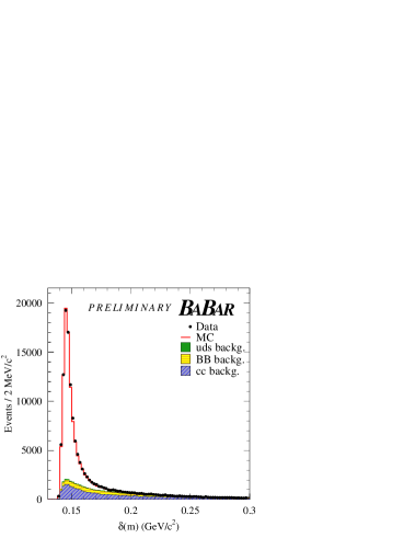
Figure 1: $\delta(m)$ distributions from data and simulated events. The signal and the different background components are indicated. MC events have been normalised to the data luminosity according to the different cross sections. The light quark component is very small and hardly visible.

3.2 $q^{2}$ measurement

The $D^{0}\rightarrow K^{-}e^{+}\nu_{e}$ is a 3-body decay and its dynamics depends on two variables. In semileptonic decays these variables are usually taken as $q^{2}$ and $\cos(\theta_{e})$. Throughout the present analysis, $q^{2}$ has been evaluated using $q^{2}=\left(p_{D}-p_{K}\right)^{2}$ $\left(=\left(p_{e}+p_{\nu_{e}}\right)^{2}\right)$ where $p_{D}$ and $p_{K}$ are the four-momenta of the $D$ and $K$ meson, respectively. The differential decay rate versus these two variables factorises in two parts depending, respectively, on $q^{2}$ and $\theta_{e}$. The variation of $d\Gamma/d\cos(\theta_{e})$ is fixed by angular momentum and helicity conservation and has a $\sin^{2}{\theta_{e}}$ dependence. The aim of the present analysis is to measure the $q^{2}$ dependence of the form factor whose shape depends on the decay dynamics.

After having applied the $D^{0}$ and $D^{*+}$ mass constrained fits, the values of the variables $q^{2}$ and $\cos(\theta_{e})$ are obtained and will be noted as $q^{2}_{r}$ and $\cos(\theta_{e})_{r}$, respectively. Background contributions in these distributions have been evaluated from corresponding distributions obtained in simulated event samples, normalized to the same integrated luminosity analyzed in data. The measured $q^{2}_{r}$ distribution is shown in Figure 2. The expected background level has been indicated and the fitted signal component, as obtained in the following, has been added.

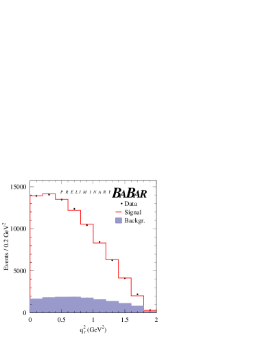
Figure 2: Distributions of $q^{2}_{r}$. Points with error bars are data. The distribution from background events is given by the blue histogram. The fitted signal component is overlayed.

The $q^{2}_{r}$ distribution for signal events is obtained by subtracting the estimated background distribution from the total measured distribution. Using simulated events the reconstruction accuracy on $q^{2}$ has been obtained by comparing reconstructed ($q^{2}_{r}$) and true simulated ($q^{2}_{s}$) values.

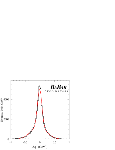
Figure 3: Distribution of the difference between the real and the reconstructed value of the $q^{2}$ variable ($\Delta q^{2}=q^{2}_{r}-q^{2}_{s}$) as obtained from simulated events. The fitted curve is the sum of two Gaussian distributions.

Figure 3 shows a double Gaussian fit to the $q^{2}$ resolution distribution. We obtain widths $\sigma_{1}=0.077~{}\rm{GeV}^{2}$ and $\sigma_{2}=0.276~{}\rm{GeV}^{2}$ for the two Gaussians, which are of similar area.

The variation of the signal efficiency as a function of $q^{2}_{s}$ is shown in Figure 4.

Figure 4: $q^{2}_{s}$ dependent efficiency after all selection requirements, from (Run1) simulated signal events.

3.3 Unfolding procedure

To obtain the unfolded $q^{2}$ distribution for signal events, corrected for resolution and acceptance effects, the Singular Value Decomposition (SVD) [8] of the resolution matrix has been used in conjunction with a regularization which minimizes the curvature of the correction distribution. A SVD of a real $m\times n$ matrix $A$ is its factorization of the form:

$$A~{}=~{}U~{}S~{}V^{T},$$

where $U$ is an $m\times m$ orthogonal matrix, $V$ is an $n\times n$ orthogonal matrix, while $S$ is an $m\times n$ diagonal matrix with non-negative elements:

$$S_{ii}=s_{i}\geq 0.$$

The quantities $s_{i}$ are called Singular Values (SV) of the matrix $A$. If the matrix of a linear system is known with some level of uncertainty, and some SV of the matrix are significantly smaller than others, the system may be difficult to solve even if the matrix has full rank, and SVD suggests a method of treating such problems. We will assume that the SV values $s_{i}$ form a non-increasing sequence.

The method uses binned distributions. It needs, as input, a 2-d array which indicates how events generated in a bin in $q^{2}_{s}$ are distributed over several bins in $q^{2}_{r}$. To be able to correct for acceptance effects one needs also the initial distribution in $q^{2}_{s}$, as given by the generator. The number of events estimated in each bin of the $q^{2}_{r}$ variable $\left(n^{i,estimated}_{q^{2}_{r}}\right)$ can be expressed as:

$$\sum_{j=1}^{m}A_{ij}w^{j}=n^{i,estimated}_{q^{2}_{r}}$$

where $w^{j}$ is an unknown deviation of the number of simulated events in bin $j$ of the $q^{2}_{s}$ variable, from the initial Monte Carlo value. $A_{ij}$ is the actual number of events which were generated in bin $j$ and ended up in bin $i$. The elements of the vector $w^{j}$ are determined by minimizing a $\chi^{2}$ expression obtained by comparing estimated and measured number of events in each $q^{2}_{r}$ bin:

$$\sum_{i=1}^{n}{\left(\frac{\sum_{j=1}^{m}{A_{ij}w^{j}-n^{i}_{q^{2}_{r}}}}{\sigma_{n^{i}_{q^{2}_{r}}}}\right)^{2}}=min,$$

where $\sigma_{n^{i}_{q^{2}_{r}}}$ is the corresponding uncertainty on the measured number of events in bin $i$. The minimization leads to the system:

$$\tilde{A}w=\tilde{n}_{q^{2}_{r}}$$ (4)

where $\tilde{A}_{ij}=A_{ij}/\sigma_{n^{i}_{q^{2}_{r}}}$ and $\tilde{n}_{q^{2}_{r}}=n^{i}_{q^{2}_{r}}/\sigma_{n^{i}_{q^{2}_{r}}}$.

The exact solution of Equation (4) will again most certainly lead to rapidly oscillating distribution. This spurious oscillatory component should be suppressed and this can be achieved by adding a regularization term to the expression to be minimized:

$$\left(\tilde{A}w-\tilde{n}\right)^{T}\left(\tilde{A}w-\tilde{n}\right)+\tau\left(Cw\right)^{T}Cw~{}=~{}min.$$

Here $C$ is a matrix which suppress solutions $w$ having large curvatures and $\tau$ determines the relative weight of this condition. The curvature of the discrete distribution $w_{j}$ is defined as the sum of the squares of its second derivatives:

$$\sum_{i}\left[\left(w_{i+1}-w_{i}\right)-\left(w_{i}-w_{i-1}\right)\right]^{2}.$$

The unfolded $q^{2}$ distribution is given by the bin-by-bin product of $w$ and of the initial Monte Carlo distribution. This approach provides the full covariance matrix for the bin contents of the unfolded distribution. Its inverse should be used for any $\chi^{2}$ calculation involving the unfolded distribution.

For a square response matrix, Singular Values (SV) correspond essentially to eigenvalues of this matrix. The number of significant SV has been obtained by looking at their distribution in experiments generated using a toy simulation of the experimental conditions, and keeping those which are above a plateau [8]. According to this procedure, four values can be retained in the present analysis.

Unfolded $q^{2}$ distributions, obtained by dividing the total sample into four similar data sets (each corresponding to about 21k events) have been analyzed. These distributions, and the total resulting sample, have been fitted using the pole and the modified pole models. Corresponding values for the parameters are given in Table 1.

It has to be noted that obtained values for $m_{\rm{pole}}$ and $\alpha_{\rm{pole}}$ are independent of a choice for a number of SV. In addition selecting a fixed number of SV results in introducing biases on the values evaluated in each bin for the unfolded distribution. Thus, at present, when providing the $q^{2}$ dependence of the hadronic form factor and the corresponding error matrix we have kept all SV (see also Section 4.5).

Table 1: Fitted values for the parameters corresponding respectively to a pole mass and a modified pole mass model for the form factor, obtained in different samples of similar statistics and for the total. The last column indicates the fraction of background events.

Data sample	$m_{\rm{pole}}$ $(\rm{GeV/}c^{2})$	$\alpha_{\rm{pole}}$	bckg. fraction
Run1	$1.808\pm 0.027$	$0.54\pm 0.06$	$16.3\%$
Run2-1	$1.889\pm 0.033$	$0.37\pm 0.07$	$16.6\%$
Run2-2	$1.847\pm 0.032$	$0.43\pm 0.07$	$16.4\%$
Run2-3	$1.864\pm 0.033$	$0.41\pm 0.07$	$16.7\%$
All	$1.854\pm 0.016$	$0.43\pm 0.03$	$16.5\%$

4 SYSTEMATIC STUDIES

Systematic uncertainties originate from non-perfect simulation of the charm fragmentation process and of the detector response, uncertainties in the control of the background level and composition, and the unfolding procedure. Differences between data and Monte Carlo in quantities used in the analysis may result in biases that need to be corrected.

These effects have been evaluated by redoing the unfolding procedure after having modified the conditions that correspond to a given parameter entering in the systematics and evaluating the variation on the value of the fitted $m_{\rm{pole}}$ and $\alpha_{\rm{pole}}$ parameters.

For some of these studies dedicated event samples have been used in which a $D^{0}$ is reconstructed in the $K^{-}\pi^{+}$ or $K^{-}\pi^{+}\pi^{0}$ decay channel.

4.1 Systematics related to $c$-quark hadronization

The signal selection is based on variables related to $c$-quark fragmentation and decay properties of signal events. As we measured differences between the hadronization properties of $c$-quarks events in real and simulated events, a $q^{2}$-dependent difference in efficiency between these two samples is expected. To have agreement between the distributions measured in real and simulated events, for the different variables entering into the Fisher analysis a weighting procedure has been used. These weights have been obtained using events with a reconstructed $D^{0}$ decaying into $K^{-}\pi^{+}$ or $K^{-}\pi^{+}\pi^{0}$. The data-MC agreement of the measured distributions indicates that uncertainties related to the tuning are below 5 $\rm{MeV/}c^{2}$ on $m_{\rm{pole}}$. These corrections correspond to a 16 $\rm{MeV/}c^{2}$ displacement on $m_{\rm{pole}}$.

4.2 Systematics related to event selection and analysis algorithm

Another study has been done by analyzing $D^{0}\rightarrow K^{-}\pi^{+}\pi^{0}$ events as if they were $K^{-}e^{+}\nu$ events. The two photons from the $\pi^{0}$ are removed from the particle lists and events are reconstructed using the algorithm applied to the semileptonic $D^{0}$ decay channel. The “missing” $\pi^{0}$ and the charged pion play, respectively, the role of the neutrino and of the electron. In the two mass constrained fits, to preserve the correct kinematic limits, it is necessary to consider that the “fake” neutrino has the $\pi^{0}$ mass and that the “fake” electron has the $\pi^{+}$ mass. With these events one can measure possible $q^{2}$-dependent effects related to some of the selection criteria and the accuracy of the measurement of $q^{2}$.

In these studies the “exact” value of $q^{2}$ is defined as $q^{2}=(p_{\pi^{+}}+p_{\pi^{0}})^{2}$. Results obtained using real and simulated events are compared to identify possible differences. Fractions of real and simulated events are selected using the Fisher discriminant variables defined to reject background events, the $\chi^{2}$ probability from the two fits, the $\delta(m)$ selection, and the requirement for having at least one spectator particle. In this selection, the Fisher variable used against the $c\overline{c}$ background does not include $\cos(\theta_{e})$ and $p_{e}$. This is because the angular distribution in $K^{-}\pi^{+}\pi^{0}$ events is close to $\cos^{2}(\theta_{\pi})$.

There is no evidence for a statistically significant different behavior in data as compared with the simulation. The statistical accuracy of this comparison, based at present on the Run1 data sample, corresponds to an uncertainty on the pole mass of $\pm 15~{}\rm{MeV/}c^{2}$.

4.3 Detector related systematics

To search for differences between real and simulated events, distributions of $\Delta q^{2}=q^{2}_{r}-q^{2}_{s}$, obtained by selecting $D^{0}\rightarrow K^{-}\pi^{+}\pi^{0}$ events in a given bin of $q^{2}_{s}$ have been compared. One notes that these distributions are systematically slightly narrower for simulated events. We have evaluated this effect to be lower than 5$\%$ and have redone the exercise after adding a smearing on $q^{2}_{r}$, in simulated events. We obtain a +4 $\rm{MeV/}c^{2}$ increase on the fitted pole mass and assign this value as a systematic error.

Effects from a momentum dependent difference between real and simulated events on the charged lepton efficiency reconstruction and on the kaon identification have been evaluated. Such differences have been measured for electrons and kaons using dedicated data samples. When applied, the corresponding corrections induce an increase of the fitted pole mass by +2 $\rm{MeV/}c^{2}$ and +4 $\rm{MeV/}c^{2}$, for electrons and kaons respectively. A relative uncertainty of 30$\%$ has been assumed on this correction.

4.4 Background related systematics

The background under the $D^{*+}$ signal has two components which have respectively a peaking and a non-peaking behavior.

The peaking background arises from events with a real $D^{*+}$ in which the slow $\pi^{+}$ is included in the candidate track combination. Its main components, as expected from the simulation, comprise events with real or fake $K^{-}$ or positron. They mainly correspond to $D^{0}\rightarrow K^{-}\pi^{0}e^{+}\nu_{e}$ and $D^{0}\rightarrow K^{-}\pi^{+}\pi^{0}$ events where, for the latter, the $\pi^{0}$ has a Dalitz decay or a converted photon.

The non-peaking background originates from non-$c\overline{c}$ events and from continuum charm events in which the $\pi$ candidate does not come from a decaying $D^{*+}$. RS combinations, for $\delta(m)>0.18~{}\rm{GeV/}c^{2}$ and WS combinations can be used to compare data and simulated event rates. It has been verified that $\delta(m)$ distributions were in agreement in the tail of RS events and reproduce well the level of WS combinations (see Figures 1 and 5).

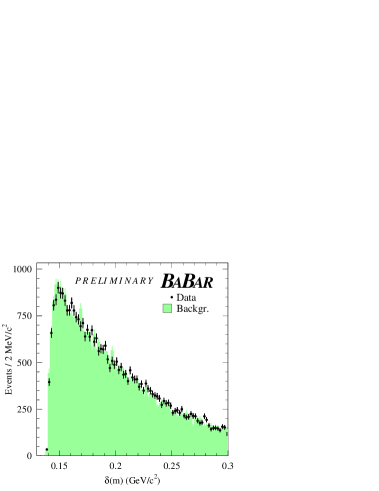
Figure 5: $\delta(m)$ distributions from data (points with error bars) and simulated events (shaded histogram) in WS $K^{-}e^{+}\pi^{-}$ events.

Table 2: Systematics corresponding to uncertainties on the level of the different background sources.

Source	variation	$\delta\left(m_{\rm{pole}}\right)$	$\delta\left(\alpha_{\rm{pole}}\right)$
	$(\%)$	$(\rm{MeV/}c^{2})$
$D^{0}\rightarrow K^{-}\pi^{0}e^{+}\nu_{e}$	$\pm 9$	$\pm 4.4$	$\mp 0.0087$
other peaking	$\pm 10$	$\pm 1.2$	$\mp 0.0023$
$c\overline{c}$ non-peaking	$\pm 10$	$\pm 3.0$	$\mp 0.0062$
$B^{+}B^{-}$	$\pm 10$	$\pm 2.6$	$\mp 0.0050$
$B^{0}\bar{B}^{0}$	$\pm 10$	$\pm 4.3$	$\mp 0.0084$
$uds$	$\pm 10$	$\pm 0.5$	$\mp 0.0010$
total		$\pm 7.4$	$\pm 0.0147$

As outlined in Table 2, each background component has been varied by $\pm 10\%$ ( a value which is larger than observed differences in the analyzed distributions), apart for the $D^{0}\rightarrow K^{-}\pi^{0}e^{+}\nu_{e}$ component for which we use $\pm 9\%$, corresponding to the combination of the PDG uncertainty with a recent measurement of this decay channel by the CLEO-c experiment [9].

4.5 Control of the statistical accuracy and of systematics in the SVD approach

For a fixed number of singular values, we verify that the statistical precision obtained for each binned unfolded value is reasonable and that biases generated by having removed information are under control.

This has been achieved by fitting the same model for the form factor, directly on the measured distribution, after having included resolution effects, and then by comparing the uncertainty obtained on the extracted parameter with the one determined by fitting the unfolded distribution using that model. These studies have been complemented by toy simulations.

One observes that the error obtained from a fit of the unfolded distribution is underestimated by a factor of $\sim 1.3$, which depends on the statistics of simulated events. Pull distributions indicate also that unfolded values in each bin are biased. The importance of the biases decreases as the number of kept singular values increases. When the number of SV is equal to the number of bins no biases are present. When the number of SV is smaller, these effects are corrected using pull results. It has been verified that these corrections, obtained for a given value of the pole mass, do not bias results expected in experiments generated with a different value for $m_{\rm{pole}}$. Corrections defined with $m_{\rm{pole}}=1.8~{}\rm{GeV/}c^{2}$ induce a shift below 4 $\rm{MeV/}c^{2}$ when applied on experiments generated with $m_{\rm{pole}}=1.7~{}{\rm or}~{}1.9~{}\rm{GeV/}c^{2}$.

4.6 Systematics summary

The systematic uncertainties evaluated on the determination of $m_{\rm{pole}}$ and $\alpha_{\rm{pole}}$ are summarized in Table 3.

Table 3: Summary of corrections and systematics on the fitted parameters. The sign of the correction is given by the sign of the difference between the fitted values after and before applying the correction.

Source	$\delta\left(m_{\rm{pole}}\right)$	$\delta\alpha_{\rm{pole}}$
	$(\rm{MeV/}c^{2})$
$c$-hadronization tuning	$-16\pm 5$	$+0.03\pm 0.01$
reconstruction algorithm	$\pm 15$	$\pm 0.03$
resolution on $q^{2}$	$+4\pm 4$	$-0.01\pm 0.01$
particle ID	$+6\pm 2$	$-0.02\pm 0.01$
background control	$\pm 7$	$\pm 0.02$
unfolding method	$\pm 5$	$\pm 0.01$
total	$-6\pm 20$	$+0.01\pm 0.04$

The systematic error matrix for the ten unfolded values has been also computed by considering, in turn, each source of uncertainty and by measuring the variation, $\delta_{i}$, of the corresponding unfolded value in each bin ($i$). The elements of the error matrix are the sum, over all sources of systematics, for the quantities $\delta_{i}\cdot\delta_{j}$. The total error matrix has been evaluated as the sum of the matrices corresponding respectively to statistical and systematic uncertainties.

5 RESULTS

In the present measurement the fit to a model has been done by comparing the number of events measured in a given bin of $q^{2}$ with the expectation from the exact analytic integration of the expression $p_{K}^{3}(q^{2})\left|f_{+}(q^{2})\right|^{2}$ over the bin range. The normalisation is left free to float and the weight matrix evaluated from SVD is used. From the measured integrated decay spectrum in each bin, the value of the form factor $|f_{+}(q^{2})|$ has been evaluated at the bin center. By convention it has been assumed that $|f_{+}(0)|=1$.

The unfolded $q^{2}$ distribution, for signal events and keeping four SV, is given in Figure 6 where it has been compared with the fitted distributions obtained using the pole and the modified pole ansatz.

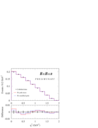
Figure 6: Comparison between the normalised unfolded $q^{2}$ distribution of the form factor obtained in the present analysis, keeping four SV, and those corresponding to the two fitted models. Lower plots give the difference between measured and fitted distributions. Vertical lines correspond to statistical uncertainties.

Results for the values of $m_{\rm{pole}}$ and $\alpha_{\rm{pole}}$ are independent of the choice of a given number of kept SV. The number of SV corresponds to the number of independent combinations of the ten bins used in the analysis. To minimize correlations between bin’s content and to compare with the $q^{2}$ distributions obtained in other experiments the distribution obtained using ten SV has been provided. The content of each bin is given in Table 4. The corresponding statistical and total error matrices are given also in that table and the $q^{2}$ variation of the hadronic form factor is displayed in Figure 7.

Table 4: Unfolded distribution using ten SV. The second line of this table gives the integrated values of the differential decay branching fraction over 0.2$(\rm{GeV}^{2})$ intervals (quoted on the first line). The total distribution has been normalised to unity for $q^{2}$ varying from 0 to 2 $(\rm{GeV}^{2})$. The statistical error matrix corresponding to the above measurements is then provided. On the diagonal is given the uncertainty on each measured value. Off-diagonal terms correspond to the correlation coefficients. Including systematics, the total error matrix is then provided.

$q^{2}$ bin	[0, 0.2]	[0.2, 0.4]	[0.4, 0.6]	[0.6, 0.8]	[0.8, 1.0]	[1.0, 1.2]	[1.2, 1.4]	[1.4, 1.6]	[1.6, 1.8]	[1.8, 2.0]
fraction	0.1999	0.1791	0.1606	0.1489	0.1007	0.0962	0.0570	0.0363	0.0201	0.0012
stat.	0.0040	-.63	.24	-.094	.034	-.0065	-.0022	0.0006	-.0025	.0002
error		0.0072	-.66	.27	-.10	.025	.0015	-.0003	.0008	-.0001
and			0.0090	-.69	.29	-.081	.011	-.0074	.0022	.0004
correl.				0.0081	-.67	.24	-.060	.025	-.0063	.0019
					0.0071	-.64	.23	-.083	.021	-.0066
						0.0056	-.64	.25	-.064	-.0035
							0.0044	-.60	.15	.022
								0.0032	-.44	-.050
									0.0018	-.059
										0.00054
total	0.0045	-.48	.23	-.097	-.0084	-.073	-.079	-.082	-.12	-.044
error		0.0073	-.65	.27	-.11	.0038	-.023	-.027	-.039	-.016
and			0.0090	-.69	.28	-.086	.0027	-.016	-.013	-.0071
correl.				0.0081	-.67	.24	-.055	.029	-.0048	.0006
					0.0071	-.62	.24	-.067	.039	-.0003
						0.0057	-.60	.27	-.028	.0075
							0.0045	-.55	.19	.041
								0.0032	-.36	-.025
									0.0019	-.0006
										0.00055

Similar measurements of the $q^{2}$ dependence of $\left|f_{+}(q^{2})\right|$ have been obtained by several experiments; recent published results are summarized in the following.

Data taken at the $\mathchar 28935\relax(4S)$ energy and corresponding to an integrated luminosity of $7$ fb^-1 have been analyzed by CLEO III [11]. Only three $q^{2}$ bins have been used because of the rather poor resolution obtained on this variable.

The FOCUS fixed target photo-production experiment has collected 12840 signal events for the decay chain: $D^{*+}\rightarrow D^{0}\pi^{+};~{}D^{0}\rightarrow K^{-}\mu^{+}\nu_{\mu}$ [12]. The $q^{2}$ resolution has a r.m.s. of $0.22~{}(\rm{GeV/}c)^{2}$.

The BELLE $B$-factory experiment has done a measurement by reconstructing all particles in the event, but the neutrino, which parameters can be obtained using kinematic constraints. As a result, they achieve a very good reconstruction accuracy of about $0.010~{}(\rm{GeV}^{2})$ on $q^{2}$ but at the price of a low overall efficiency. Analyzing 282 fb^-1 integrated luminosity, they select about 2500 $D^{0}\rightarrow K^{-}\mu^{+}\nu_{\mu}$ and $D^{0}\rightarrow K^{-}e^{+}\nu_{e}$ events with low background levels.

In Table 5 results obtained by the different collaborations have been summarized when fitting a pole mass and a modified pole mass $q^{2}$ distributions for the form factor.

Table 5: Fitted values for $m_{\rm{pole}}$ and $\alpha_{\rm{pole}}$ models for the form factor.

Experiment	$m_{\rm{pole}}$ $(\rm{GeV/}c^{2})$	$\alpha_{\rm{pole}}$	Statistics
CLEO III [11]	$1.89\pm 0.05^{+0.04}_{-0.08}$	$0.36\pm 0.10^{+0.08}_{-0.07}$	$7$ fb-1
FOCUS [12]	$1.93\pm 0.05\pm 0.03$	$0.28\pm 0.08\pm 0.07$	13k events
BELLE [13]	$1.82\pm 0.04\pm 0.03$	$0.52\pm 0.08\pm 0.06$	$282$ fb-1
BABAR	$1.854\pm 0.016\pm 0.020$	$0.43\pm 0.03\pm 0.04$	$75$ fb-1

Results obtained in this analysis on the $q^{2}$ variation of the hadronic form factor have been compared in Figure 7 with FOCUS [12] measurements and with the lattice QCD [3] evaluation.

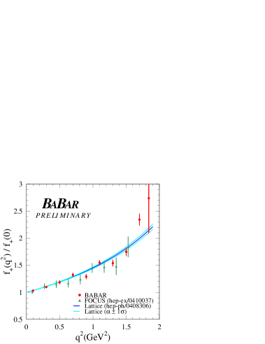
Figure 7: Comparison between the measured variation of $<|f_{+}(q^{2})|>$ obtained in the present analysis and in the FOCUS experiment. The band corresponds to lattice QCD [3] expectations.

The present result is valid in the limit that in real events the radiative component has the same characteristics as in the simulation which uses the PHOTOS generator program. With the level of accuracy of present measurements better studies of radiative effects are needed.

6 SUMMARY

Fitting the pole mass and the modified pole mass ansatz to the measurements, we obtain preliminary values for the single parameter that governs their $q^{2}$ dependence:

$$m_{\rm{pole}}=(1.854\pm 0.016\pm 0.020)~{}\rm{GeV/}c^{2}$$ (5)

$$\alpha_{\rm{pole}}=0.43\pm 0.03\pm 0.04~{}~{}~{}~{}~{}~{}~{}~{}$$

where the first error is statistical and the second systematic. The effective $m_{\rm{pole}}$ value is rather different from $m_{D_{s}^{*+}}$ indicating large corrections to naive expectations. In the modified pole model this can be interpreted as evidence for the contribution from other vector states of invariant mass higher than the $D_{s}^{*+}$ mass.

The value measured for $\alpha_{\rm{pole}}$ agrees, within errors, with the one obtained from lattice QCD [3]: $\alpha_{\rm{pole}}^{\rm{lattice}}=0.50\pm 0.04$. We provide also a preliminary $q^{2}$ distribution of the form factor, corrected for effects from reconstruction efficiency and finite resolution measurements.

7 ACKNOWLEDGMENTS

The authors wish to thank C. Bernard and D. Becirevic for a clarification on the way to compare the values of the modified pole parameter $(\alpha_{\rm{pole}})$ obtained from lattice QCD and from direct measurements.

We are grateful for the extraordinary contributions of our PEP-II colleagues in achieving the excellent luminosity and machine conditions that have made this work possible. The success of this project also relies critically on the expertise and dedication of the computing organizations that support BABAR. The collaborating institutions wish to thank SLAC for its support and the kind hospitality extended to them. This work is supported by the US Department of Energy and National Science Foundation, the Natural Sciences and Engineering Research Council (Canada), Institute of High Energy Physics (China), the Commissariat à l’Energie Atomique and Institut National de Physique Nucléaire et de Physique des Particules (France), the Bundesministerium für Bildung und Forschung and Deutsche Forschungsgemeinschaft (Germany), the Istituto Nazionale di Fisica Nucleare (Italy), the Foundation for Fundamental Research on Matter (The Netherlands), the Research Council of Norway, the Ministry of Science and Technology of the Russian Federation, and the Particle Physics and Astronomy Research Council (United Kingdom). Individuals have received support from the Marie-Curie IEF program (European Union) and the A. P. Sloan Foundation.

References

-
[1]
J.G. Koerner and G.A. Schuler, Z. Phys. C 38, 511 (1988);
Erratum-ibid, C 41, 690 (1989).
M. Bauer and M. Wirbel, Z. Phys. C 42, 671 (1989). - [2] D. Becirevic and A.B. Kaidalov, Phys. Lett. B 478, 417 (2000).
- [3] C. Aubin et al., Phys. Rev. Lett. 94, 011601 (2005) [arXiv:hep-ph/0408306].
- [4] E. Barberio and Z. Was, Comput. Phys. Commun. 79, 291 (1994).
- [5] The BABAR Collaboration, B. Aubert et al., Nucl. Instrum. Methods A 479, 1 (2002).
- [6] G. C. Fox and S. Wolfram, Phys. Rev. Lett. 41, 1581 (1978).
- [7] R.A. Fisher, Ann. Eugenics 7, 179 (1936).
- [8] A. Hoecker and V. Kartvelishvili, Nucl. Inst. Meth. A 372, 469 (1996) [arXiv:hep-ph/9509307].
- [9] T.E. Coan et al., CLEO collaboration, Phys. Rev. Lett. 95, 181802 (2005) [arXiv:hep-ex/0506052].
-
[10]
N. Isgur and D. Scora, Phys. Rev. D 52, 2783 (1995)
[arXiv:hep-ph/9503486],
N. Isgur, D. Scora, B. Grinstein and M.B. Wise, Phys. Rev. D 39, 799 (1989). - [11] G.S. Huang et al., CLEO collaboration, Phys. Rev. Lett. 94, 011802 (2005) [arXiv:hep-ex/0407035].
- [12] J.M. Link et al., FOCUS collaboration, Phys. Lett. B 607, 233 (2005) [arXiv:hep-ex/0410037].
- [13] L. Widhalm et al., BELLE collaboration [arXiv:hep-ex/0604049].