We present a combined measurement of the Cabibbo-Kobayashi-Maskawa matrix element $|V_{cb}|$ and of the parameters $\rho^{2}$, $R_{1}$, and $R_{2}$, which fully characterize the form factors of the $B^{0}\rightarrow D^{*-}\ell^{+}\nu_{\ell}$ decay in the framework of HQET, based on a sample of about 52,800 $B^{0}\rightarrow D^{*-}\ell^{+}\nu_{\ell}$ decays recorded by the BABAR detector. The kinematical information of the fully reconstructed decay is used to extract the following values for the parameters (where the first errors are statistical and the second systematic): $\rho^{2}=1.156\pm 0.094\pm 0.028$, $R_{1}=1.329\pm 0.131\pm 0.044$, $R_{2}=0.859\pm 0.077\pm 0.022$, $\mathcal{F}(1)|V_{cb}|=(35.03\pm 0.39\pm 1.15)\times 10^{-3}$. By combining these measurements with the previous BABAR measurements of the form factors which employs a different technique on a partial sample of the data, we improve the statistical accuracy of the measurement, obtaining: $\rho^{2}=1.179\pm 0.048\pm 0.028,R_{1}=1.417\pm 0.061\pm 0.044,R_{2}=0.836\pm 0.037\pm 0.022,$ and $\mathcal{F}(1)|V_{cb}|=(34.68\pm 0.32\pm 1.15)\times 10^{-3}.$ Using the lattice calculations for the axial form factor $\mathcal{F}(1)$, we extract $|V_{cb}|=(37.74\pm 0.35\pm 1.25\pm^{1.23}_{1.44})\times 10^{-3}$, where the third error is due to the uncertainty in $\mathcal{F}(1)$.

Submitted to the 33^rd International Conference on High-Energy Physics, ICHEP 06,

26 July—2 August 2006, Moscow, Russia.

1 INTRODUCTION

The study of the $B^{0}\rightarrow D^{*-}\ell^{+}\nu_{\ell}$ decay [1] is interesting in many respects. In the Standard Model of electroweak interactions the rate of this weak decay is proportional to the absolute square of the Cabibbo-Kobayashi-Maskawa (CKM) matrix element $V_{cb}$, which measures the weak coupling of the $b$ to the $c$ quark. Therefore the determination of the branching ratio of this decay allows for a determination of $|V_{cb}|$.

The decay is also influenced by strong interactions, whose effect can be parameterized through two axial form factors ${\cal A}_{1}$ and ${\cal A}_{2}$, and one vector form factor $V$, each of which depend on the momentum transfer $q^{2}$ of the $B$ meson to the $D^{*}$ meson. The form of this dependence is not known a priori. Equivalently, instead of $q^{2}$, the linearly related quantity $w$, which is the product of the four-velocities of the $\kern 1.79993pt\overline{\kern-1.79993ptB}{}^{0}$ and $D^{*+}$, defined in Eq. (1), can be used.

In the heavy-quark effective field theory (HQET) framework [2, 3], these three form factors are related to each other through heavy quark symmetry (HQS), but HQET allows for three free parameters which must be determined by experiment.

Several experiments have measured $|V_{cb}|$ based on the study of the differential decay width $d\Gamma/dw$ of $B^{0}\rightarrow D^{*-}\ell^{+}\nu_{\ell}$ decays [4, 5, 6, 7, 8, 9, 10]. They determine only one of the parameters of the HQET from their data, while they rely on the CLEO measurement of the other two, as described in Ref. [11]. This is the largest systematic uncertainty common to all previous measurements of $|V_{cb}|$ based on this method.

Improved measurements of all parameters are also important for describing the dominant background from $b\rightarrow c\rightarrow\ell$ cascades in both inclusive and exclusive $b\rightarrow u\ell\nu$ decays for measurements of $|V_{ub}|$. These motivations have been the basis of the measurement of all three parameters performed by BABAR and presented in Ref. [12]. While a new value of $|V_{cb}|$ has been computed using the new results as input to the previous measurement, the full correlation between $|V_{cb}|$ and the three form factor parameters cannot be fully accounted for in that approach.

In the present analysis, we perform a simultaneous measurement of both $|V_{cb}|$ and of the form factor parameters from the measurement of the full four-dimensional differential decay rate (see Sec. 2). We extend the method of Ref. [10] by combining the measurement of different one-dimensional decay rates, fully accounting for the correlations between them, to extract the whole set of observables.

A brief outline of the paper is as follows: In Sec. 2, we introduce the definition of all used observables, form factors, form factor combinations, and parameters. In Sec. 3 we briefly describe the relevant aspects of the detector and datasets we utilize in this measurement. In Sec. 4 we describe event reconstruction and selection and in Sec. 5 the analysis method. Sec. 6 describes fit results and the estimation of systematic uncertainties. In Sec. 7 we summarize the results of this analysis and combine form factor measurements with a previous BABAR measurement to arrive at a further improvement of the statistical errors, both for the form factor parameters and for the measurement of $|V_{cb}|$.

2 FORMALISM

This section outlines the formalism and describes the parameterization used for the form factors. More details can be found in Refs. [2, 3]. The lowest order quark-level diagram for the decay $B^{0}\rightarrow D^{*-}\ell^{+}\nu_{\ell}$ is shown in Fig. 1.

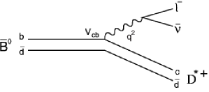
Figure 1: Quark-level diagram showing the weak interaction vertices in the decay $B^{0}\rightarrow D^{*-}\ell^{+}\nu_{\ell}$.

2.1 Kinematic variables

The decay $B^{0}\rightarrow D^{*-}\ell^{+}\nu_{\ell}$ is completely characterized by four variables, three angles and $q^{2}$, the square of the momentum transfer from the $B$ to the $D^{*}$ meson.

The momentum transfer is linearly related to another Lorentz-invariant variable, called $w$, by

$$w\equiv v_{B}\cdot v_{D^{*}}={p_{B}\cdot p_{D^{*}}\over m_{B}m_{D^{*}}}={m_{B}^{2}+m_{D^{*}}^{2}-q^{2}\over 2m_{B}m_{D^{*}}},$$ (1)

where $m_{B}$ and $m_{D^{*}}$ are the masses of the $B$ and the $D^{*}$ mesons, $p_{B}$ and $p_{D^{*}}$ are their four-momenta, and $v_{B}$ and $v_{D^{*}}$ are their four-velocities. In the $B$ rest frame the expression for $w$ reduces to the Lorentz boost $\gamma_{D^{*}}=E_{D^{*}}/M_{D^{*}}$.

The ranges of $w$ and $q^{2}$ are restricted by the kinematics of the decay, with $q^{2}\approx 0$ corresponding to

$$w_{max}=\frac{m_{B}^{2}+m_{D^{*}}^{2}}{2m_{B}m_{D^{*}}}\approx 1.504$$ (2)

and $w_{min}=1$ corresponding to

$$q_{max}^{2}=(m_{B}-m_{D^{*}})^{2}\approx 10.69~{}({\mathrm{\,Ge\kern-1.00006ptV\!/}c^{2}})^{2}.$$ (3)

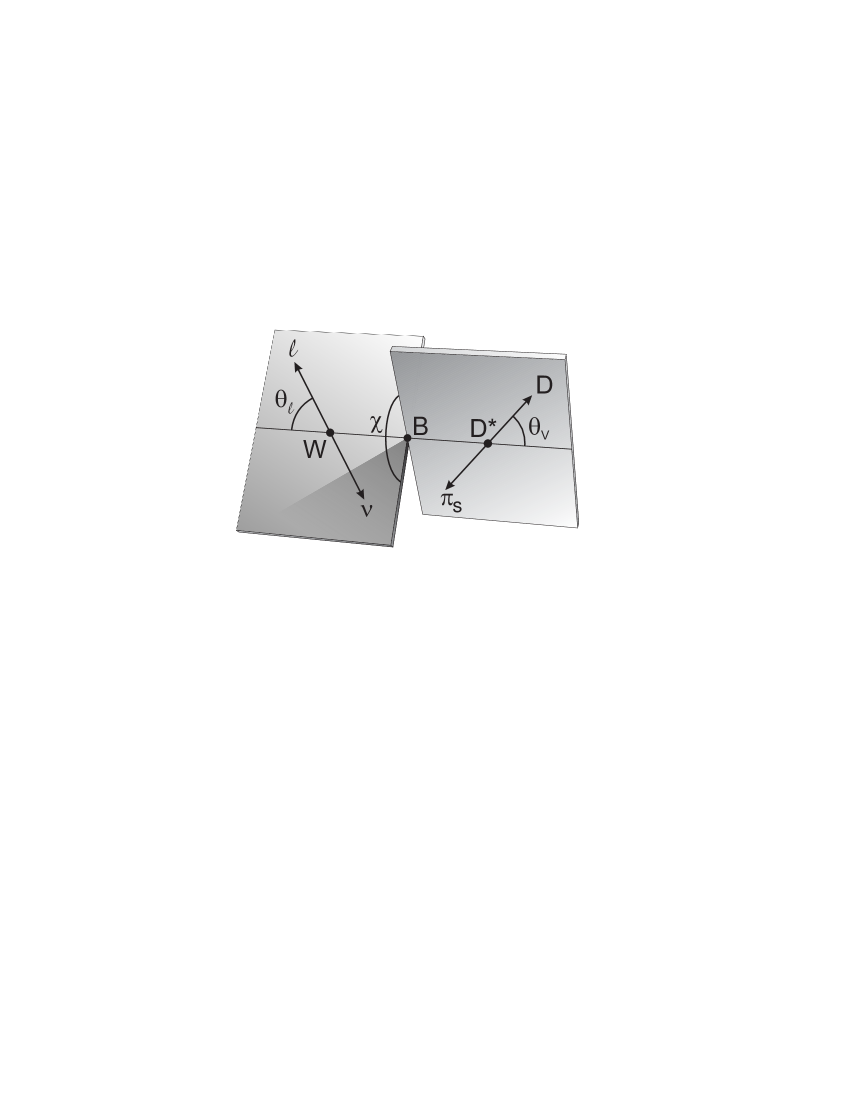
Figure 2: Kinematics of a $B^{0}\rightarrow D^{*-}\ell^{+}\nu_{\ell}$ decay, mediated by an intermediate vector boson $W$; $\pi_{s}$ is the soft pion from the $D^{*}$ decay. This diagram defines the three angles ${\theta_{\ell}}$, ${\theta_{V}}$ and ${\chi}$.

In this analysis we only reconstruct the decay $D^{*+}\rightarrow D^{0}\pi^{+}$, where $D^{0}\rightarrow K\pi$, $D^{0}\rightarrow K\pi\pi\pi$ or $D^{0}\rightarrow K\pi\pi^{0}$. The angular variables, shown in Fig. 2, are

• ${\theta_{\ell}}$, the angle between the direction of the lepton in the virtual $W$ rest frame and the direction of the virtual $W$ in the $B$ rest frame,

• ${\theta_{V}}$, the angle between the direction of the $D$ in the $D^{*}$ rest frame and the direction of the $D^{*}$ in the $B$ rest frame,

• ${\chi}$, the dihedral angle between the plane formed by the $D^{*}-D$ and the plane formed by the $W-\ell$ system.

2.2 Four-dimensional decay distribution

The Lorentz structure of the $B^{0}\rightarrow D^{*-}\ell^{+}\nu_{\ell}$ decay amplitude can be expressed in terms of three helicity amplitudes ($H_{+}$, $H_{-}$, and $H^{0}_{0}$), which correspond to the three polarization states of the $D^{*}$ (two transverse and one longitudinal). For light leptons these amplitudes are expressed [2, 3] in terms of the three form factors $h_{A_{1}}$, $R_{1}$ and $R_{2}$:

$$H_{i}(w)=m_{B}\dfrac{R^{*}(1-r^{2})(w+1)}{2\sqrt{1-2wr+r^{2}}}h_{A_{1}}(w)\tilde{H}_{i}(w),$$ (4)

where

$$\tilde{H}_{\mp} = \dfrac{\sqrt{1-2wr+r^{2}}\biggl{(}1\pm\sqrt{\dfrac{w-1}{w+1}R_{1}(w)}\biggr{)}}{1-r}$$ (5)

$$\tilde{H}_{0} = 1+\dfrac{(w-1)(1-R_{2}(w))}{1-r}$$ (6)

where $R^{*}=\dfrac{2\sqrt{m_{B}m_{D^{*}}}}{m_{B}+m_{D^{*}}}$ and $r=\dfrac{m_{D^{*}}}{m_{B}}$.

The full differential decay rate in terms of the three helicity amplitudes is [2, 3]:

$$\dfrac{\mathrm{d\Gamma}(B^{0}\rightarrow D^{*-}\ell^{+}\nu_{\ell})}{\mathrm{d}w\mathrm{d\cos\theta_{\ell}}\mathrm{d\cos\theta_{V}}\mathrm{d\chi}} = \dfrac{6m_{B}m_{D^{*}}^{2}r\sqrt{w^{2}-1}(1-2wr+r^{2})}{8(4\pi)^{4}}$$

$$\times G_{F}^{2}|V_{cb}|^{2}\bigl{[}(1-\cos\theta_{\ell})^{2}\sin^{2}\theta_{V}H^{2}_{+}(w)\biggr{.}$$

$$+ (1+\cos\theta_{\ell})^{2}\sin^{2}\theta_{V}H^{2}_{-}(w)$$

$$+ 4\sin^{2}\theta_{\ell}\cos^{2}\theta_{V}H^{2}_{0}(w)$$

$$- 2\sin^{2}\theta_{\ell}\sin^{2}\theta_{V}\cos 2\chi H_{+}(w)H_{-}(w)$$

$$- 4\sin\theta_{\ell}(1-\cos\theta_{\ell})\sin\theta_{V}\cos\theta_{V}\cos\chi\times H_{+}(w)H_{0}(w)$$

$$+ \biggl{.}4\sin\theta_{\ell}(1+\cos\theta_{\ell})\sin\theta_{V}\cos\theta_{V}\cos\chi\times H_{-}(w)H_{0}(w)\bigr{]},$$

where all three of the $H_{i}$ are functions of $w$. The four-dimensional distribution of $w$, ${\cos\theta_{\ell}}$, ${\cos\theta_{V}}$, and $\chi$ described by Eq. (2.2) is the physical observable from which we extract the form factors. The normalization of this distribution is directly related to $|V_{cb}|$.

2.3 Form-factors parameterizations

The HQET does not predict the functional form of the form factors, and one needs a parameterization of these form factors. In the limit of infinite mass for the $b$ and $c$ quark, $R_{1}$ and $R_{2}$ are simply both equal to 1. Corrections to this approximation are calculated in powers of $({\mathchar 28931\relax_{{\rm QCD}}}/{m_{Q}})$ and $\alpha_{S}$.

Parameterizations as a power expansion in $(w-1)$ have been proposed in literature. The first linear parameterization is given by:

$$h_{A_{1}}(w) = h_{A_{1}}(1)(1-\rho^{2}(w-1))\,.$$ (8)

A generic second order extension can be realized adding an extra parameter $c$ as coefficient of the $(w-1)^{2}$ term:

$$h_{A_{1}}(w) = h_{A_{1}}(1)(1-\rho^{2}(w-1)+c(w-1)^{2}).$$ (9)

In both cases $R_{1}$ and $R_{2}$ are considered to be constants, neglecting their $w$ dependence.

Among various predictions relating the coefficients of higher order terms to that of the linear term, we decided to adopt the Caprini, Lellouch and Neubert [13] one (in the following referred to as CLN); the authors find the following functional forms for the three HQET form factors:

$$h_{A_{1}}(w) = h_{A_{1}}(1)\big{[}1-\rho^{2}_{h_{A_{1}}}z+(53\rho^{2}_{h_{A_{1}}}-15)z^{2}\big{.}$$

$$\big{.}-(231\rho^{2}_{h_{A_{1}}}-91)z^{3}\big{]},$$

$$R_{1}(w) = R_{1}(1)-0.12(w-1)+0.05(w-1)^{2},$$

$$R_{2}(w) = R_{2}(1)+0.11(w-1)-0.06(w-1)^{2},$$

where:

$$z=\dfrac{\sqrt{w+1}-\sqrt{2}}{\sqrt{w+1}+\sqrt{2}}\,.$$ (11)

These functional forms are determined apart from three unknown parameters, $\rho^{2}_{h_{A_{1}}}$, $R_{1}(1)$ and $R_{2}(1)$, which must be extracted from the data.

It is important to notice that $h_{A_{1}}(1)\equiv\mathcal{F}(1)$, corresponding to the value of the Isgur-Wise function evaluated at zero recoil (using the notation commonly found in literature for $d\Gamma/dw$). A recent lattice calculation [14] (including a QED correction of 0.7%) gives: $h_{A_{1}}(1)=\mathcal{F}(1)=0.919^{+0.030}_{-0.035}$.

3 THE BABAR DETECTOR

The BABAR detector is described in detail in Ref. [15]. The momenta of charged particles are measured by a tracking system consisting of a five-layer silicon vertex tracker (SVT) and a 40-layer drift chamber (DCH), operating in a 1.5-T solenoidal magnetic field. Charged particles of different masses are distinguished by their energy loss in the tracking devices and by a ring-imaging Cherenkov detector. Electromagnetic showers from electrons and photons are measured in a CsI(Tl) calorimeter. Muons are identified in a set of resistive plate chambers inserted in the iron flux-return yoke of the magnet.

The analysis is based on a data sample of 79 $\mbox{\,fb}^{-1}$ recorded on the $\mathchar 28935\relax{(4S)}$ resonance, and 9.6 $\mbox{\,fb}^{-1}$ recorded 40 MeV below it, with the BABAR detector [15] at the PEP-II asymmetric-energy $e^{+}e^{-}$ collider. We use samples of GEANT Monte Carlo (MC) [16] simulated events that correspond to about three times the data sample size.

4 RECONSTRUCTION AND EVENT SELECTION

The reconstruction of the events is the same as used in Ref. [10], and the event selection is an improved version of the one used in that paper.

We select events that contain a $D^{*+}$ candidate and an oppositely charged electron or muon with momentum $1.2<p_{\ell}<2.4~{}{\mathrm{\,Ge\kern-1.00006ptV\!/}c}$. Unless explicitly stated otherwise, momenta are measured in the $\mathchar 28935\relax{(4S)}$ rest frame, which does not coincide with the laboratory frame due to the boost of the PEP-II beams. In this momentum range, the electron (muon) efficiency is about 90% (60%) and the hadron misidentification rate is typically 0.2% (2.0%). We select $D^{*+}$  candidates in the momentum range $0.5<p_{D^{*}}<2.5~{}{\mathrm{\,Ge\kern-1.00006ptV\!/}c}$ in the channel $D^{*+}\rightarrow D^{0}{\pi_{s}^{+}}$, with the $D^{0}$ decaying to $K^{-}\pi^{+},~{}K^{-}\pi^{+}\pi^{-}\pi^{+}$, or $K^{-}\pi^{+}\pi^{0}$. The charged hadrons of the $D^{0}$ candidate are fitted to a common vertex and the candidate is rejected if the fit probability is less than $0.1\%$. We require the invariant mass of the hadrons to be compatible with the $D^{0}$ mass within $\pm 2.5$ times the experimental resolution. This corresponds to a range of $\pm 34{\mathrm{\,Me\kern-1.00006ptV\!/}c^{2}}$ for the $D^{0}\rightarrow K^{-}\pi^{+}\pi^{0}$ decay and $\pm 17{\mathrm{\,Me\kern-1.00006ptV\!/}c^{2}}$ for the other decays. For the decay $D^{0}\rightarrow K^{-}\pi^{+}\pi^{0}$, we accept only candidates from portions of the Dalitz plot where the square of the decay amplitude, as determined by Ref. [17], is at least 10$\%$ of the maximum it attains anywhere in the plot. For the soft pion from the $D^{*+}$ decay, $\pi_{s}^{+}$, the momentum in the laboratory frame must be less than 450 ${\mathrm{\,Me\kern-1.00006ptV\!/}c}$, and the transverse momentum greater than 50 ${\mathrm{\,Me\kern-1.00006ptV\!/}c}$. Finally, the lepton, the ${\pi_{s}^{+}}$, and the $D^{0}$ are fitted to a common vertex using a beam-spot constraint, and the probability for this fit is required to exceed 1%.

In semileptonic decays, the presence of an undetected neutrino complicates the separation of the signal from background. We compute a kinematic variable with considerable power to reject background by determining, for each $B$-decay candidate, the cosine of the angle between the momentum of the $\kern 1.79993pt\overline{\kern-1.79993ptB}{}^{0}$ and of the $D^{*+}\ell^{-}$ pair, under the assumption that only a massless neutrino is missing:

$$\cos{\theta_{B^{0},D^{*}\ell}}=\frac{2E_{\kern 1.25995pt\overline{\kern-1.25995ptB}{}^{0}}E_{D^{*}\ell}-M^{2}_{\kern 1.25995pt\overline{\kern-1.25995ptB}{}^{0}}-M^{2}_{D^{*}\ell}}{2p_{\kern 1.25995pt\overline{\kern-1.25995ptB}{}^{0}}p_{\raisebox{-0.90417pt}{\scriptsize$D^{*}\ell$}}}.$$

This quantity constrains the direction of the $\kern 1.79993pt\overline{\kern-1.79993ptB}{}^{0}$ to lie along a cone whose axis is the direction of the $D^{*+}\ell^{-}$ pair, but with an undetermined azimuthal angle about the cone axis. The value of $w$ varies with this azimuthal angle; we take the average of the minimum and maximum values as our estimator $\tilde{w}$ for $w$. This results in a resolution of $0.04$ on $w$. We divide the sample into 10 bins in $\tilde{w}$  from 1.0 to 1.5, with the last bin extending to the kinematic limit of 1.504.

The selected events are divided into six subsamples, corresponding to the two leptons and the three $D^{0}$ decay modes. In addition to signal events, each subsample contains background events from six different sources:

• combinatoric (events from $B\kern 1.79993pt\overline{\kern-1.79993ptB}{}$ and continuum in which at least one of the hadrons assigned to the $D^{*+}$ does not originate from the $D^{*+}$ decay);

• continuum ($D^{*+}\ell^{-}$ combinations from $e^{+}e^{-}\rightarrow c\bar{c}$);

• fake leptons (combined with a true $D^{*+}$);

• uncorrelated background ($\ell$ and $D^{*+}$ produced in the decay of two different $B$ mesons);

• events from charged $B$ background, $B^{+}\rightarrow D^{*}\ell^{+}\nu_{\ell}X$ (via $B^{+}\rightarrow\overline{D}^{**0}\ell^{+}\nu_{\ell}$ or non-resonant $B^{+}\rightarrow D^{*-}\ell^{+}\nu_{\ell}\pi^{+}$ production), and neutral $B$ background $B^{0}\rightarrow D^{*-}\ell^{+}\nu_{\ell}X$, (via $B^{0}\rightarrow D^{**-}\ell^{+}\nu_{\ell}$ or non-resonant $B^{0}\rightarrow D^{*-}\ell^{+}\nu_{\ell}\pi^{0}$ production);

• and correlated background events due to the processes $\kern 1.79993pt\overline{\kern-1.79993ptB}{}^{0}\rightarrow D^{*+}\bar{\nu}\tau^{-},~{}\tau^{-}\rightarrow\ell^{-}X$ and $\kern 1.79993pt\overline{\kern-1.79993ptB}{}^{0}\rightarrow D^{*+}X_{c},~{}X_{c}\rightarrow\ell^{-}Y$.

We estimate the correlated background (which amounts to be less than 0.5% of the selected candidates) from the Monte Carlo simulation based on measured branching fractions [19, 20], while we determine all others from data. Except for the combinatoric background, all other background sources exhibit a peak in the ${\Delta M}=M_{D^{*+}}-M_{D^{0}}$ distribution, where $M_{D^{*+}}$ and $M_{D^{0}}$ are the measured $D^{*+}$ and $D^{0}$ candidate masses.

We determine the composition of the subsamples in each $\tilde{w}$  bin in two steps. First we estimate the amount of combinatoric, continuum, and fake-lepton background by fitting the $\Delta M$ distributions in the range $0.139<{\Delta M}<0.165~{}{\mathrm{\,Ge\kern-1.00006ptV\!/}c^{2}}$ simultaneously to three sets of events: data recorded on resonance, data taken below the $\mathchar 28935\relax{(4S)}$ (thus containing only continuum background), and data in which tracks that fail very loose lepton-selection criteria are taken as surrogates for fake leptons. The distributions are fitted with the sum of three Gaussian functions with a common mean and different widths to describe $D^{*+}\rightarrow D^{0}{\pi_{s}^{+}}$ decays and with empirical functions

$$F_{comb}({\Delta M})=\frac{1}{N}\,\left[1-e^{\left(-\frac{{\Delta M}-{\Delta M}_{0}}{c_{1}}\right)}\right]\,\left(\frac{{\Delta M}}{{\Delta M}_{0}}\right)^{c_{2}}$$ (12)

based on simulation for the combinatoric background. The four parameters of the Gaussian functions are common, while the fraction of peaking background events and the parameters describing the combinatoric background differ for the signal, off-peak, and fake-lepton samples.

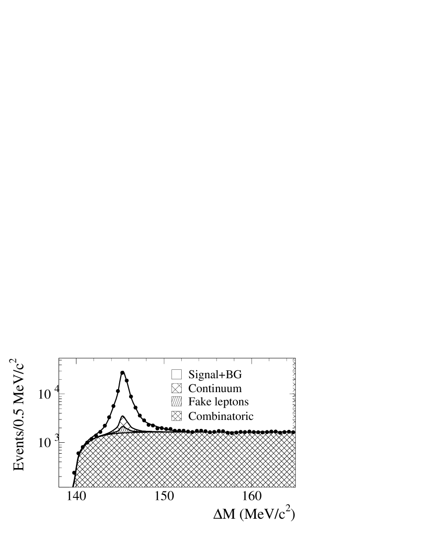
Figure 3: Yields of on-resonance data (points) and the results of the fit (line) to the $\Delta M$ distribution, with contributions from continuum, fake-lepton, and combinatoric-$D^{*+}$ background events summed over all $\tilde{w}$  bins.

Since the $\Delta M$ resolution depends on whether or not the $\pi_{s}^{+}$ track is reconstructed only in the SVT or in the SVT and DCH, the fits are performed separately for these two classes of events. We rescale the number of continuum and fake-lepton events in the mass range $0.143<{\Delta M}<0.148~{}{\mathrm{\,Ge\kern-1.00006ptV\!/}c^{2}}$, based on the relative on- and off-resonance luminosity and measured hadron misidentification probabilities. The fit is performed in multiple steps: the combinatoric background is first fixed to the simulation prediction in order to optimize the fit of the signal in the tail region around the peak. Then the peak shape is fixed to the fitted one, and the combinatoric background is left free to float, to allow for possible small deviations from the simulation.

In the subsequent analysis we fix the fraction of combinatoric, fake-lepton, and continuum events in each $\tilde{w}$  bin to the values obtained following the procedure described above. Figure 3 shows the $\Delta M$ fit results for the on-resonance data.

In a second step, we fit the $\cos{\theta_{B^{0},D^{*}\ell}}$ distributions in the range $-10<\cos{\theta_{B^{0},D^{*}\ell}}<5$ and determine the signal contribution and the normalization of the uncorrelated and $B\rightarrow D^{*}\ell^{+}\nu_{\ell}X$ background events. Neglecting resolution effects, signal events meet the constraint $|\cos{\theta_{B^{0},D^{*}\ell}}|\leq 1$, while the distribution of $B\rightarrow D^{*}\ell^{+}\nu_{\ell}X$ events extends below $-1$, and the distribution of the uncorrelated background events is spread over the entire range considered.

We perform the fit separately for each $\tilde{w}$  bin, with the individual shapes for the signal and for each of the six background sources taken from MC simulation, specific for each of the six subsamples. Signal events are generated with the CLN form factor parameterization, tuned to the results from CLEO [11]. Radiative decays ($\kern 1.79993pt\overline{\kern-1.79993ptB}{}^{0}\rightarrow D^{*+}\ell^{-}\kern 1.79993pt\overline{\kern-1.79993pt\nu}{}_{\ell}$$\gamma$) are modeled by PHOTOS [22] and are treated as signal. $B\rightarrow D^{**}\ell\nu$ decays involving orbitally excited charm mesons are generated according to the ISGW2 model [24], and decays with non-resonant charm states are generated following the prescription in Ref. [25]. To reduce the sensitivity to statistical fluctuations we require that the ratio of $B\rightarrow D^{*}\ell^{+}\nu_{\ell}X$ and of uncorrelated background events to the signal be the same for all three $D^{0}$ decay modes and for the electron and muon samples. Fit results are shown in Fig. 4. In total, there are 68,840 events in the range $|\cos{\theta_{B^{0},D^{*}\ell}}|<1.2$. The average fraction of signal events is $(76.7\pm 0.3)$%, where the error is only statistical.

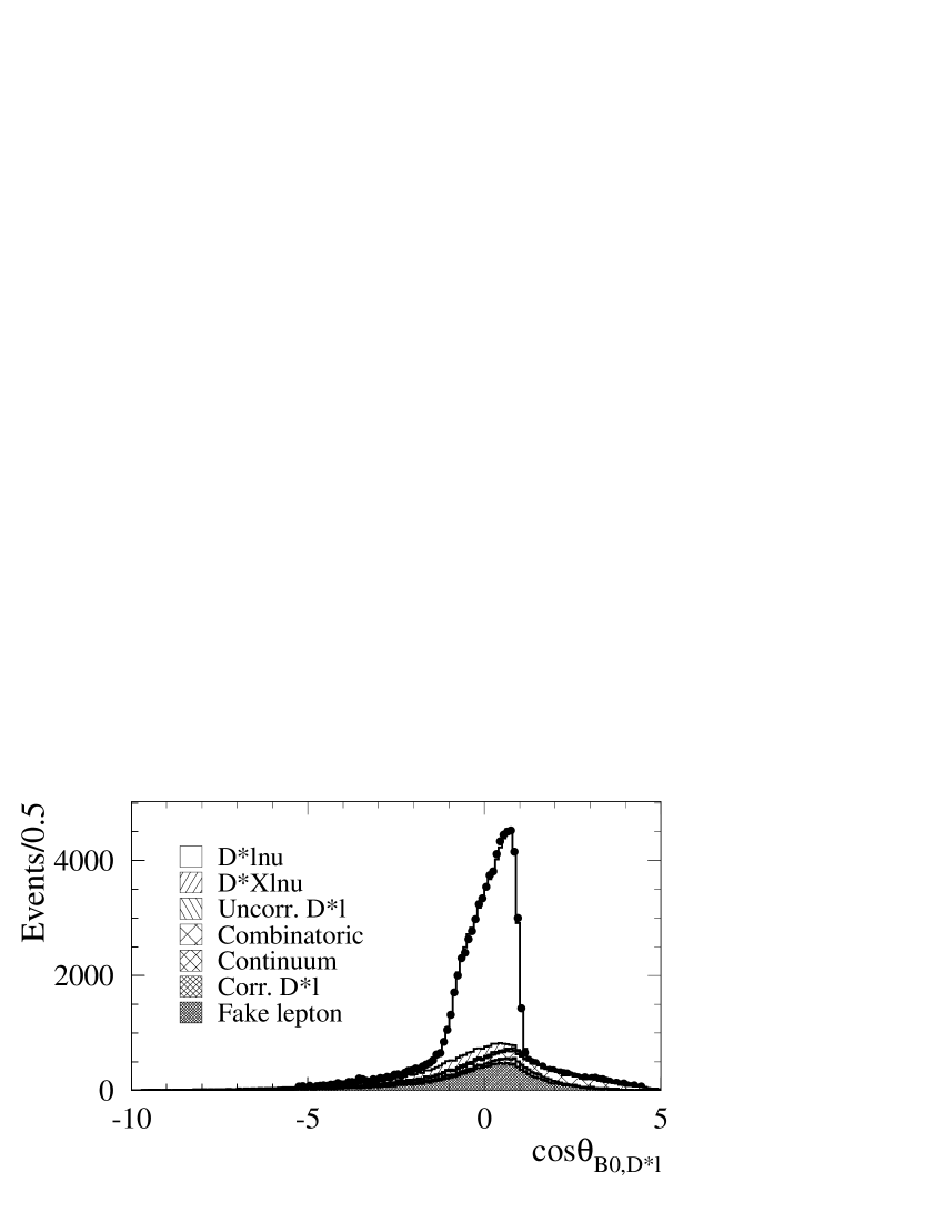
Figure 4: Yields of on-resonance data (points) and the results of the fit (histograms) to the $\cos{\theta_{B^{0},D^{*}\ell}}$ distribution, summed over all $\tilde{w}$  bins.

5 THE EXTRACTION OF $|V_{cb}|$ AND THE FORM FACTOR PARAMETERS

The approach followed in this analysis to simultaneously measure $|V_{cb}|$ and the three form factor parameters is to extend the one-dimensional fit procedure of Ref. [10] to several one-dimensional distributions, while fully accounting for the mutual correlations, using the same sample of selected events. This permits disentangling the effects coming from each of the parameters, and to measure all of them.

In principle, the multi-dimensional phase space could be divided into several independent bins, and the fraction of signal events in each of them could be determined as described in the previous section. In practice, the need for a detailed bin segmentation would imply serious statistical limitations in most of the bins. For this reason, we instead consider projections of the data into the most significant variables ( $w$, ${\cos\theta_{\ell}}$, ${\cos\theta_{V}}$). We divide each projection into ten bins, and determine the amount of signal events in each bin applying the procedure described above. We then fit the resulting projections to extract the form factors and $|V_{cb}|$. We account for the correlations between bins of different projections by noting that the covariance between the content of two bins in different one-dimensional distributions is given by the common number of events in these bins, while it is zero for bins in the same distribution.

Any kinematic observable sensitive to the form factor parameters can be used, the sensitivity to $|V_{cb}|$ being already present in the $w$ distribution alone. We have studied the distributions of the kinematic observables describing the decay, as discussed in Sec. 2. We have verified that the distribution of $\chi$ is practically insensitive to the form factor parameter changes, therefore we have chosen $w$, ${\cos\theta_{\ell}}$ and ${\cos\theta_{V}}$ as set of observables to be included in the fit. Figure 5 shows the sensitivity of each of the 4 kinematical variables describing the $B^{0}\rightarrow D^{*-}\ell^{+}\nu_{\ell}$ decay to the form factor parameters.

The value of $|V_{cb}|$ and the form factor parameters are extracted from a least squares fit to the set of measurements given by the measured contents of bins of $w$, ${\cos\theta_{\ell}}$ and ${\cos\theta_{V}}$, according to the selection described in Sec. 4 and the cut $|\cos{\theta_{B^{0},D^{*}\ell}}|<1.2$. The $w$ and ${\cos\theta_{V}}$ distributions are divided into ten equal size bins. The ${\cos\theta_{\ell}}$ distribution is divided in the analysis in 10 non-equal size bins, whose boundaries are $[-1.0,-0.4,-0.2,0.0,0.2,0.4,0.5,0.6,0.7,0.8,1.0]$, chosen according to the strong variations in the shape, and therefore to the available statistics.

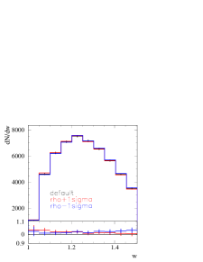
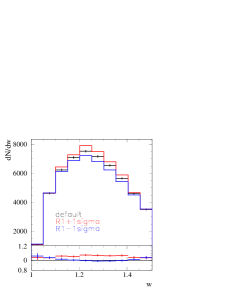
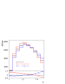
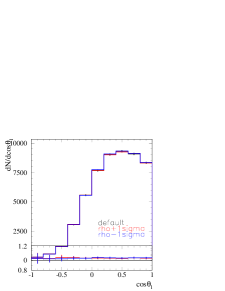
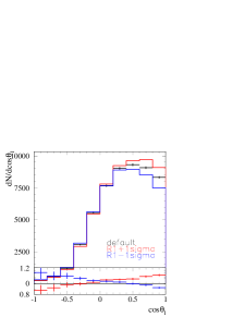
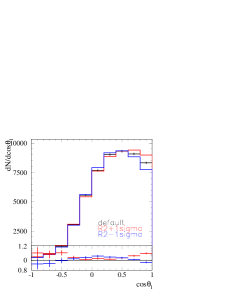
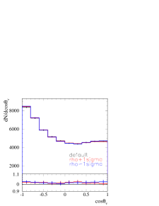
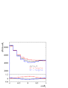
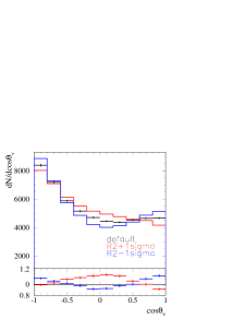
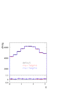
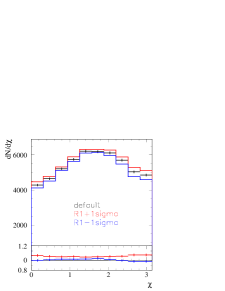
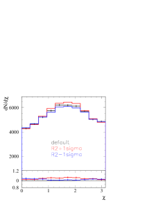
Figure 5: Sensitivity of the $w$, ${\cos\theta_{\ell}}$, ${\cos\theta_{V}}$ and $\chi$ variables to the variations of the three form factor parameters $\rho^{2}$, $R_{1}$ and $R_{2}$. The variations considered are 1 $\sigma$ for $\rho^{2}$, $R_{1}$, and $R_{2}$ using the measured value from [10] for $\rho^{2}$ and from Ref. [11] for the others.

5.1 The fit method

The $\chi^{2}$ function to be minimized is an extension of the one used in Ref. [10]. Defining $n$ as the total number of observable bins, $N_{i}^{data}$ the total number of observed events in bin $i$, $N_{i}^{bkg}$ the number of estimated background events for that bin, and $N_{i}^{MC}$ the number of simulated signal events falling in that bin, the $\chi^{2}$ can be written as:

$$\chi^{2} = \sum_{i=1}^{n}\sum_{j=1}^{n}\biggl{(}N_{i}^{data}-N_{i}^{bkg}-\sum_{k=1}^{N_{i}^{MC}}\mbox{W}_{i}^{k}\biggr{)}\times$$

$$C_{ij}^{-1}\biggl{(}N_{j}^{data}-N_{j}^{bkg}-\sum_{k=1}^{N_{i}^{MC}}\mbox{W}_{j}^{k}\biggr{)}$$

where $\mbox{W}_{i}^{k}$ is the weight assigned to the $k$-th simulated signal event falling into bin $i$ in order to evaluate the expected signal yield as a function of the searched parameters, and $C_{ij}$ is the covariance matrix element for the bin pair $ij$.

Each weight $\mbox{W}_{i}^{k}$ is the product of four weights, $\mbox{W}_{i}^{k}=\mbox{W}^{\mathcal{L}}\mbox{W}_{i}^{\epsilon,k}\mbox{W}_{i}^{S,k}\mbox{W}_{i}^{ff,k}$. The factor $\mbox{W}^{\mathcal{L}}$ accounts for the normalization of data and simulation samples. It depends on the total number of $B\bar{B}$ events, $N_{B\bar{B}}=(85.9\pm 0.9)\times 10^{6}$, on the fraction of $B^{0}\bar{B}^{0}$ events, $f_{00}=0.489\pm 0.012$ [19], on the branching fraction $\mathcal{B}(D^{*+}\rightarrow D^{0}\pi^{+})=0.677\pm 0.005$ [19], and on the $B^{0}$ lifetime $\tau_{B^{0}}=1.532\pm 0.009$ ps [19]. The factor $\mbox{W}_{i}^{\epsilon,k}$ accounts for differences in reconstruction and particle-identification efficiencies predicted by the Monte Carlo simulation and measured with data, as a function of particle momentum and polar angle.

The factor $\mbox{W}_{i}^{S,k}$ accounts for potential small residual differences in efficiencies for the six data subsamples (3 $D^{0}$ decay modes and 2 leptons) and allows for adjustment of the $D^{0}$ branching fractions, properly dealing with the correlated systematic uncertainty. It is the product of several scale factors that are floating parameters in the fit, each constrained to an expected value with a corresponding experimental error. To account for the uncertainty in the multiplicity-dependent tracking efficiency, we introduce a factor $\mbox{W}_{trk}^{S}=1+N_{trk}(1-\delta_{trk})$, where $N_{trk}$ is the number of charged tracks in the $D^{*}\ell$ candidates in each sample and $\delta_{trk}$ is constrained to one within the estimated uncertainty in the single-track efficiency of $0.8$%. Similarly, multiplicative correction factors are introduced to adjust lepton ($\delta_{PID\,e}$, $\delta_{PID\,\mu}$) efficiencies, kaon efficiencies in the different selections used for different $D^{0}$ decay channels ($\delta_{PID\,K\,tight}$, $\delta_{PID\,K\,not\,a\,pion}$), and $\pi^{0}$ ($\delta_{\pi^{0}}$) efficiencies, within the total estimated uncertainties of these efficiencies, and $D^{0}$ branching fractions ($\delta_{BR\,D^{0}\,K\pi}$, $\delta_{BR\,D^{0}\,K\pi\pi\pi}$, $\delta_{BR\,D^{0}\,K\pi\pi^{0}}$). Correlations between the branching fractions are taken into account in the constraint through the covariance matrix $C_{BR}$ (given by the uncertainties and the correlation matrix obtained from Ref. [19, 20]). Therefore $\mbox{W}_{i}^{S,k}$ can be written as:

$$\mbox{W}_{i}^{S,k}=\delta_{PID\,e}\delta_{PID\,\mu}\delta_{PID\,K}^{i,k}(1+N_{trk}^{i,k}(1-\delta_{trk}))\delta_{\pi^{0}}^{i,k}\delta_{BR\,D^{0}}^{i,k}$$ (14)

where the kaon and $\pi^{0}$ efficiency corrections, the decay multiplicity $N_{trk}$ and the $D^{0}$ branching ratio correction depend on the particular event $k$ of the bin $i$ considered (because of the different decay multiplicity, branching ratio, kaon selector and presence of $\pi^{0}$). The addition of the constraints effectively adds extra terms to the above $\chi^{2}$ expression for each of the corrective factors $\delta$. The complete $\chi^{2}$ function used in the fit therefore is:

$$\chi^{2} = \sum_{i=1}^{n}\sum_{j=1}^{n}\biggl{(}N_{i}^{data}-N_{i}^{bkg}-\sum_{k=1}^{N_{i}^{MC}}\mbox{W}_{i}^{k}\biggr{)}\times C_{ij}^{-1}\biggl{(}N_{j}^{data}-N_{j}^{bkg}-\sum_{k=1}^{N_{i}^{MC}}\mbox{W}_{j}^{k}\biggr{)}$$

$$+\frac{(1-\delta_{PID\,e})^{2}}{\sigma_{PID\,e}^{2}}+\frac{(1-\delta_{PID\,\mu})^{2}}{\sigma_{PID\,\mu}^{2}}$$

$$+\frac{(1-\delta_{PID\,K\,tight})^{2}}{\sigma_{PID\,K\,tight}^{2}}+\frac{(1-\delta_{PID\,K\,not\,a\,pion})^{2}}{\sigma_{PIDK\,not\,a\,pion}^{2}}$$

$$+\frac{(1-\delta_{trk})^{2}}{\sigma_{trk}^{2}}+\frac{(1-\delta_{\pi^{0}})^{2}}{\sigma_{\pi^{0}}^{2}}$$

$$+\sum_{m=K\pi,K\pi\pi\pi,K\pi\pi^{0}}\sum_{n=K\pi,K\pi\pi\pi,K\pi\pi^{0}}\delta_{BR\,D^{0}\,m}\times C_{BR\,D^{0}\,mn}^{-1}\delta_{BR\,D^{0}\,n}$$

The addition of these extra terms allows us to fit all subsamples simultaneously fully taking into account the correlated systematic uncertainties, and effectively propagates these uncertainties through the weights to the uncertainty on the free parameters of the fit.

The fourth factor $\mbox{W}_{i}^{ff,k}$ accounts for the dependence of the signal yield on the parameters to be fitted. The $|V_{cb}|$ dependence is trivially given by the ratio $|V_{cb}|^{2}/|V_{cb}^{MC}|^{2}$, where the denominator is the actual value used in the simulation, derived from the branching ratio used for the decay $B^{0}\rightarrow D^{*-}\ell^{+}\nu_{\ell}$. In an analogous way the dependence on the form factor parameters ($\rho^{2}$, $R_{1}$, and $R_{2}$) is given by the ratio of the differential decay rate of Eq. (2.2) evaluated at the variable values (in the chosen fitting model) and at the simulation values (where the linear model was used).

One important point is that not all bins of all used observables can be used at the same time: in fact, once all bins belonging to one observable are used, the overall normalization is fixed, therefore for the other observables one of the bins has to be dropped, since its content and covariance matrix part can be written as linear combination of all others. The choice of the bins to be dropped is arbitrary, and it has been verified that by dropping different bins exactly the same numerical results were obtained (within the numerical precision of the fit).

Summarizing, three observables are used in the fit, $w$, $\cos\theta_{\ell}$, and $\cos\theta_{V}$, whose ranges are divided into ten bins. One bin is excluded from the fit for the last two observables, for a total of 28 bins used in the $\chi^{2}$.

This fit procedure has been tested on a signal toy Monte Carlo, and no evidence for systematic biases has been observed.

5.2 The observables’ covariance matrix

A direct consequence of this method is that the covariance matrix for the measurements corresponding to the bins used is not diagonal, since the bins are not all statistically independent. The total covariance matrix is the sum of 3 separate matrices: one for the measured data yields, one for the estimated signal yield, and one for the evaluated background. The diagonal elements of the matrices are given by the uncertainty on the bin content itself: the covariance of bins belonging to the same observable is zero, the covariance of bins from different observables is the variance of the number of events that is common between the bins.

The observed data matrix is built assuming the bin contents and their intersections obeying a Poisson distribution, therefore the variance of a bin content or of the content of the intersection of two bins is the content itself. The estimated signal matrix is built in an analogous way, where the variance of a number of weighted events $n$ is approximated by the sum of the squared weights $\sum_{i=1,n}w_{i}^{2}$.

The calculation of the background covariance matrix is less straightforward. The diagonal part is simply the estimated variance of the measured background, according to the whole procedure described in Sec. 4. The background extraction procedure does not directly determine the common number of events between two bins, because this procedure is based on a complex sequence of shapes and yield fits.

The solution adopted is to use the number of common background events between two bins as predicted by the simulation, after it has been corrected for tracking and PID efficiencies, and rescaled in such a way as to get for each bin of one of the studied kinematic observables (one among $w,{\cos\theta_{\ell}},{\cos\theta_{V}},\chi$) the background amount estimated from the data-based background evaluation. In this estimation procedure also the $\chi$ projection is used, in order to provide an additional check on the background evaluated from the three distributions used in the fit.

Since the total integral of the background measured is not exactly the same when evaluated for different kinematic observables, it has to be fixed to a given value. The average normalization determined from the four kinematic observables describing the event is used.

The spread of the background normalization values is found to be about two times larger than the estimated uncertainty from the background procedure error propagation. This is due to the fact that the uncertainties on the signal and background shapes are not accounted for in the background estimate. Taking into account the structure of the distribution of the four integrals, split into two subgroups of compatible values, the global background uncertainty is estimated to be the average of the maximum and minimum difference between these two groups (i.e., $w$ and ${\cos\theta_{\ell}}$ on one side, ${\cos\theta_{V}}$ and $\chi$ on the other). The background uncertainties are suitably rescaled in order to give the uncertainty on the integral equal to the one estimated as explained.

6 THE FIT RESULTS AND SYSTEMATIC UNCERTAINTIES

6.1 Results of the fit

The analysis result is obtained using the background covariance matrix evaluated from the measurement in the variable $w$. Table 1 shows the best fit result. The uncertainties have been determined by the MINOS [21] algorithm, whose output has been symmetrized. The $\delta$ coefficients describing systematic uncertainties not common to all events are found to be consistent with 1 within the estimated uncertainties. The contribution to the overall uncertainty due to statistical fluctuations of the data and simulated samples has been obtained by recomputing the covariance matrix of the fit after fixing all the $\delta$ parameters at their best fit values.

Figure 6 shows the distributions of the kinematical observables describing the $B^{0}\rightarrow D^{*-}\ell^{+}\nu_{\ell}$ decay with the simulation prediction computed using the best fit values for $|V_{cb}|$ and for the form factors.

The $B^{0}\rightarrow D^{*-}\ell^{+}\nu_{\ell}$ decay branching ratio is shown in the last row of the Table 1. The uncertainties are obtained through the propagation of the ones on $\rho^{2},R_{1},R_{2}$ and $\mathcal{F}(1)|V_{cb}|$, taking into account their correlations.

Parameter	Best value	$\sigma_{tot}$	$\sigma_{stat}$	$\sigma_{syst}$
$\rho^{2}$	1.156	0.095	0.094	0.004
$R_{1}$	1.329	0.131	0.131	0.007
$R_{2}$	0.859	0.077	0.077	0.002
$\mathcal{F}(1)|V_{cb}|\times 10^{3}$	35.03	0.95	0.39	0.86
BR($B^{0}\rightarrow D^{*-}\ell^{+}\nu_{\ell}$) %	4.83	0.24	0.05	0.24

Table 1: Fit result for the standard analysis. $\sigma_{tot}$ is the total uncertainty, and the last two columns show its splitting in statistical and systematic contributions (from $\delta$ parameters). In the last row the results for the branching ratio of $B^{0}\rightarrow D^{*-}\ell^{+}\nu_{\ell}$ obtained from the fit results are shown.

Table 2 shows the correlation matrix for the standard analysis result.

	$\rho^{2}$	$R_{1}$	$R_{2}$	$\mathcal{F}(1)|V_{cb}|\times 10^{3}$
$\rho^{2}$	$+1.000$	$+0.864$	$-0.922$	$-0.028$
$R_{1}$	$+0.864$	$+1.000$	$-0.928$	$-0.226$
$R_{2}$	$-0.922$	$-0.928$	$+1.000$	$+0.172$
$\mathcal{F}(1)|V_{cb}|\times 10^{3}$	$-0.028$	$-0.226$	$+0.172$	$+1.000$

Table 2: Total correlation matrix for the standard analysis fit.

The goodness of fit can be evaluated directly from the value of the fit function in the minimum, since it is based on a least squares method, obtaining a $\chi^{2}$/d.o.f. = 23.99/24 corresponding to a $\chi^{2}$ probability of 46.2%. In this evaluation the number of degrees of freedom is considered equal to the number of used bins, ignoring the bin correlations, minus the number of fitted parameters. It is interesting also to check the goodness of the fit on the separate distributions entering the fit (i.e., $w$, ${\cos\theta_{\ell}}$ and ${\cos\theta_{V}}$), considering for each of them all ten bins in which their ranges have been subdivided. The corresponding results are given in Table 3.

Variable	$\chi^{2}$/d.o.f.	$\chi^{2}$ probability
$w$	3.62/10	96.3%
$\cos\theta_{\ell}$	12.93/10	22.8%
$\cos\theta_{V}$	6.04/10	81.2%

Table 3: Goodness of fit for the distributions entering the fit for the standard analysis. All ten bins are considered.

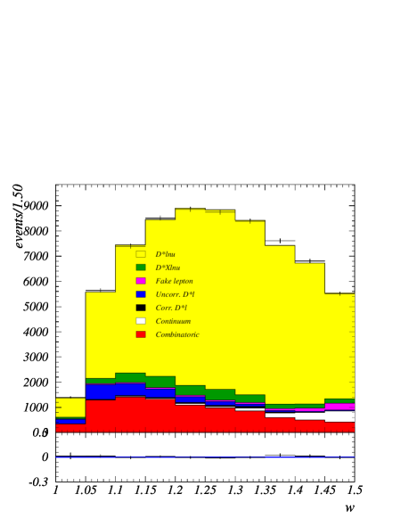
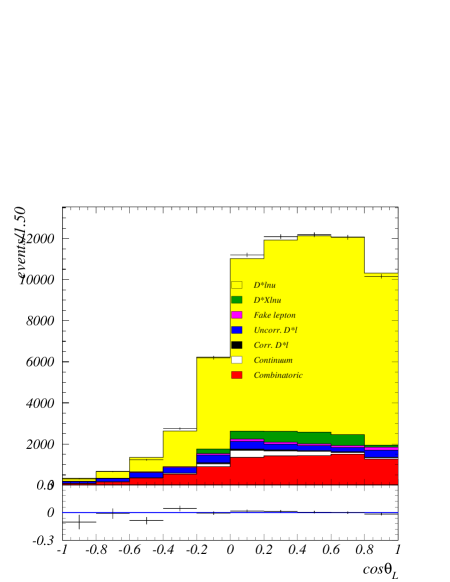
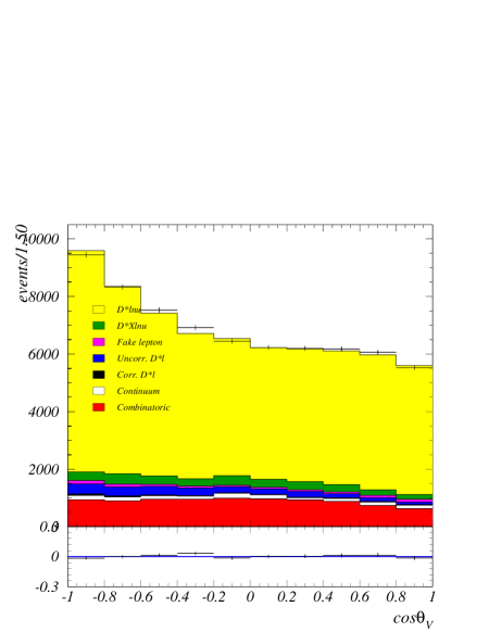
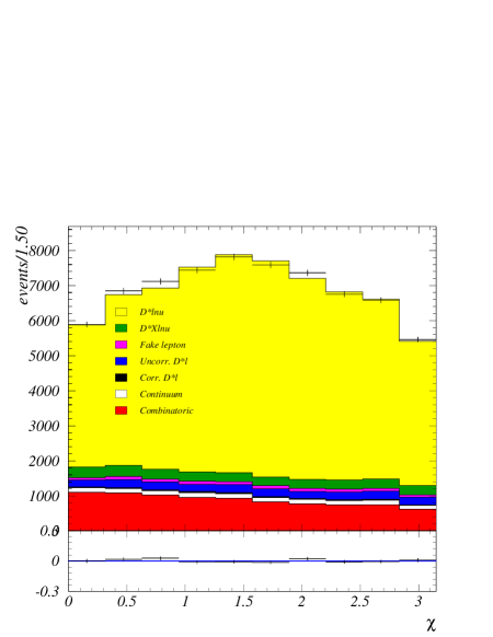
Figure 6: Distributions of $w$, $\cos\theta_{\ell}$, $\cos\theta_{V}$, $\chi$ after the fit. The error bars represent the measured values, the colored histograms represent the background estimate and the fitted signal MC. The bottom plots show the ratio between the measurement and the sum of all background and fitted signal MC events.

In Fig. 7 the contour plot at the 39% C.L. ($\Delta\chi^{2}=1$) in the $\rho^{2}$-$R_{1}$, $\rho^{2}$-$R_{2}$, $R_{1}$-$R_{2}$, $\rho^{2}$-$\mathcal{F}(1)|V_{cb}|\times 10^{3}$, $R_{1}$-$\mathcal{F}(1)|V_{cb}|\times 10^{3}$, $R_{2}$-$\mathcal{F}(1)|V_{cb}|\times 10^{3}$ planes are shown, illustrating the correlations among the variables.

Figure 7: Contour plot at 39% C.L. ($\Delta\chi^{2}=1$) in the $\rho^{2}$-$R_{1}$, $\rho^{2}$-$R_{2}$, $\rho^{2}$-$\mathcal{F}(1)|V_{cb}|\times 10^{3}$, $R_{1}$-$R_{2}$, $R_{1}$-$\mathcal{F}(1)|V_{cb}|\times 10^{3}$, $R_{2}$-$\mathcal{F}(1)|V_{cb}|\times 10^{3}$ planes (keeping the $\delta$ parameters for the systematics at their best fit values).

6.2 Systematic uncertainties

The summary of systematic uncertainties on the measured parameters is presented in Table 4. In the last column, the uncertainty breakdown for the $B^{0}\rightarrow D^{*-}\ell^{+}\nu_{\ell}$ branching ratio is also shown.

CLN	$\rho^{2}$	$R_{1}$	$R_{2}$	$\mathcal{F}(1)|V_{cb}|\times 10^{3}$	BR($B^{0}\rightarrow D^{*-}\ell^{+}\nu_{\ell}$)
stat. error	0.094	0.131	0.077	0.39	0.05
PID, trk, BR $D^{0}$	0.004	0.007	0.002	0.86	0.24
$\pi$ soft	0.013	0.005	0.001	0.46	0.18
$D^{*}l$ vertex	0.014	0.010	0.008	0.06	0.06
$B$ mom.	0.013	0.040	0.017	0.29	0.14
rad. corr.	0.005	0.004	0.000	0.19	0.07
$D^{**}$ compos.	0.011	0.008	0.009	0.10	0.07
background cov. matrix	0.006	0.004	0.002	0.04	0.04
partial sum	0.027	0.043	0.021	1.04	0.35
$B^{0}$ lifetime	-	-	-	0.10	0.03
$B\bar{B}$ number	-	-	-	0.19	0.05
BR($D^{*}\rightarrow D^{0}\pi$)	-	-	-	0.13	0.04
$f_{++}/f_{00}$	0.008	0.010	0.006	0.41	0.15
tot. syst. error	0.028	0.044	0.022	1.15	0.39

Table 4: Breakdown of systematics uncertainties.

6.2.1 Statistical, PID and tracking efficiency and $D^{0}$ branching fraction uncertainties

The uncertainty on the parameters given by the fit is not of purely statistical origin, since the systematic uncertainty sources which are not common to all events (PID efficiency, tracking efficiency, and $D^{0}$ branching fraction uncertainties) are taken directly into account in the fit through the $\delta$ coefficients appearing in the weights $\mbox{W}_{i}^{S,k}$. The splitting between statistical and systematic part of the fit result uncertainty is obtained by computing the purely statistical covariance matrix (by fixing all $\delta$ parameters at their best value) and subtracting it from the global one.

6.2.2 Soft pion efficiency

The uncertainty coming from the soft pion efficiency correction is determined by propagating the uncertainties of the parameters of the efficiency correction function. In addition, an overall efficiency uncertainty due to track reconstruction and selection is considered (a scale factor affecting only $\mathcal{F}(1)|V_{cb}|$), its magnitude being 1.3%. The two uncertainties are added in quadrature.

6.2.3 $D^{*}l$ vertex reconstruction efficiency

The uncertainty coming from the vertex reconstruction method used to select the $D^{*}l$ system has been evaluated using two alternative choices to the standard method: the first corresponds to removing the beam spot constraint from the vertex fit, while the second corresponds to removing the lepton information from the vertex fit. The biggest variation is taken as the systematic uncertainty.

6.2.4 $B$ momentum

A correction to the $B$ momentum in the simulation has to be applied to obtain agreement with data. Effectively this implies rescaling the $\cos\theta_{B^{0},D^{*}\ell}$ value determined for the simulation by a 0.97 factor. Half of the relative effect of the correction is considered as systematic uncertainty on it.

6.2.5 Radiative corrections

Radiative corrections to the $B^{0}\rightarrow D^{*-}\ell^{+}\nu_{\ell}$ decay are computed in the simulation by PHOTOS [22], which describes the final state photon radiation (FSR) up to $\mathcal{O}(\alpha^{2})$. In the event reconstruction no attempt to recover photons emitted in the decay is performed, therefore the simulated prediction of the reconstructed event is sensitive to the detail of the radiative corrections. This is particularly important in the $\cos{\theta_{B^{0},D^{*}\ell}}$ fit for electrons, where the FSR is responsible for the long tail at low values.

No detailed calculation of the full $\mathcal{O}(\alpha)$ radiative corrections to the $B^{0}\rightarrow D^{*-}\ell^{+}\nu_{\ell}$ decay is available in literature. Recently, a new $\mathcal{O}(\alpha)$ calculation of radiative corrections in kaon decays has become available [23] explicitly taking into account radiated photons, and a new detailed comparison with PHOTOS has been presented. From this comparison it is evident that the radiated photon’s energy spectrum is quite well reproduced by PHOTOS, the main difference being in the angular distribution of the photons with respect to the lepton.

In order to assess the systematic uncertainty due to the imperfect treatment of the radiative corrections, we have used the comparison presented in Ref. [23] to reweight our simulated events in order to reproduce the photon angular spectrum given there, for photons above 10 MeV in the $B$ center of mass. The effect of the reweighting has been used as an estimate of the systematic uncertainty. In this approach the possible effect of the $B^{0}$ decay form factors on the FSR description is completely ignored.

6.2.6 $B\rightarrow D^{*}\ell^{+}\nu_{\ell}X$ background description

The shapes of the different components of the $B\rightarrow D^{*}\ell^{+}\nu_{\ell}X$ background are taken from the simulation. In order to account for the uncertainty on their knowledge, the fit has been performed using only one of them at a time. The study has been performed for the $D^{0}\rightarrow K\pi$ subsample only, and assumed to be valid for all subsamples. The uncertainty on the result is given by half of the biggest variation observed.

6.2.7 Fit covariance matrix

The effect of using the background shape evaluated in different projections to compute the background covariance matrix is used as an evaluation of the corresponding systematic uncertainty (the background overall normalization is fixed to the average of the one computed in the projections). The maximal variation with respect to the basic result when changing the projection used is taken as an estimate.

6.2.8 Global normalization factors

In the second part of Table 4 the effect of the uncertainty on quantities which are normalization factors is shown. The effect of the uncertainties in the $D^{0}$ branching ratios has already been discussed, and it affects all parameters because it is changing the relative amount of signal events coming from different $D^{0}$ decays. On the other hand, the $B^{0}$ lifetime, the $D^{*}\rightarrow D^{0}\pi$ branching ratio, and the $B\bar{B}$ measured number are global scale factors affecting only $\mathcal{F}(1)|V_{cb}|$. The uncertainty on the ratio $f_{++}/f_{00}=\mathcal{B}(\mathchar 28935\relax(4S)\rightarrow B^{+}B^{-})/\mathcal{B}(\mathchar 28935\relax(4S)\rightarrow B^{0}\bar{B}^{0})$ affects both the absolute number of measured $B^{0}\rightarrow D^{*-}\ell^{+}\nu_{\ell}$ decays (and therefore $\mathcal{F}(1)|V_{cb}|$) and the relative ratio of background events from $B^{0}$ and $B^{\pm}$ in the simulation. This second aspect influences the $\cos{\theta_{B^{0},D^{*}\ell}}$ shapes and therefore the background determination. For this reason this uncertainty source cannot be considered a pure scale uncertainty affecting only $\mathcal{F}(1)|V_{cb}|$, but it touches also the form factors parameters. The analysis has been repeated by changing the $f_{++}/f_{00}$ value by one sigma and the variation has been used as systematic uncertainty on the results from this source. The $B^{0}$ lifetime used is $\tau_{B^{0}}=1.532\pm 0.009$ [19]. The $D^{*}\rightarrow D^{0}\pi$ branching ratio used is $67.7\pm 0.5\%$. The $f_{++}/f_{00}$ value used is $1.055\pm 0.055$ from Ref. [18]. The systematic uncertainty on the number of $B\bar{B}$ ($N_{B\bar{B}}$) is 1.1%. The uncertainties on these input quantities are propagated to the final fit results.

7 CONCLUSIONS

7.1 Summary of results of this analysis

A sample of about 52800 fully reconstructed $B^{0}\rightarrow D^{*-}\ell^{+}\nu_{\ell}$ decays collected by the BABAR detector has been used to measure both $\mathcal{F}(1)|V_{cb}|$ and the form factor parameters in the CLN parameterization [13] $\rho^{2}$, $R_{1}$, and $R_{2}$ in a global fit. Both identified electrons and muons have been used, the $D^{*-}$ candidates are reconstructed from the $D^{*-}$ $\rightarrow$ $\kern 1.99997pt\overline{\kern-1.99997ptD}{}^{0}$ $\pi^{-}$ decay and the $\kern 1.99997pt\overline{\kern-1.99997ptD}{}^{0}$ candidate is reconstructed in three different decay modes $K^{-}\pi^{+}$, $K^{-}\pi^{+}\pi^{+}\pi^{-}$ and $K^{-}\pi^{+}\pi^{0}$.

The obtained results are (where the first errors are statistical and the second systematic):

$$\mathcal{F}(1)|V_{cb}| = (35.03\pm 0.39\pm 1.15)\times 10^{-3}$$

$$\rho^{2} = 1.156\pm 0.094\pm 0.028$$

$$R_{1} = 1.329\pm 0.131\pm 0.044$$

$$R_{2} = 0.859\pm 0.077\pm 0.022$$

The correlations between the fitted parameters are:

$$\rho(\rho^{2},R_{1}) = +86\%$$

$$\rho(\rho^{2},R_{2}) = -92\%$$

$$\rho(\rho^{2},\mathcal{F}(1)|V_{cb}|) = -3\%$$

$$\rho(R_{1},R_{2}) = -92\%$$

$$\rho(R_{1},\mathcal{F}(1)|V_{cb}|) = -23\%$$

$$\rho(R_{2},\mathcal{F}(1)|V_{cb}|) = +17\%$$

Using a recent lattice calculation [14] ($h_{A_{1}}(1)=\mathcal{F}(1)=0.919^{+0.030}_{-0.035}$) results in the following value for $|V_{cb}|$:

$$|V_{cb}|=(38.12\pm 0.42\pm 1.25^{+1.24}_{-1.45})\times 10^{-3},$$

where the third error is due to the uncertainty in $\mathcal{F}(1)$.

The corresponding branching fraction for the decay $B^{0}\rightarrow D^{*-}\ell^{+}\nu_{\ell}$ is found to be:

$$\mathcal{B}(B^{0}\rightarrow D^{*-}\ell^{+}\nu_{\ell})=(4.84\pm 0.05\pm 0.39)\%.$$

7.2 Combination of results with alternate form factor parameters measurement

The BABAR collaboration recently published a measurement [12] of the same form factor parameters in $B^{0}\rightarrow D^{*-}\ell^{+}\nu_{\ell}$ decays based on an unbinned maximum likelihood fit to the four-dimensional decay distribution using a subset of the data analyzed in this work. This earlier analysis has a higher sensitivity to the form factor parameters and resulted in $\rho^{2}=1.145\pm 0.066\pm 0.035$, $R_{1}=1.396\pm 0.070\pm 0.027,$ and $R_{2}=0.885\pm 0.046\pm 0.013$.

We can combine the two form factor parameters measurements taking into account the correlation between them and obtain

$$\mathcal{F}(1)|V_{cb}| = (34.68\pm 0.32\pm 1.15)\times 10^{-3}$$

$$\rho^{2} = 1.179\pm 0.048\pm 0.028$$

$$R_{1} = 1.417\pm 0.061\pm 0.044$$

$$R_{2} = 0.836\pm 0.037\pm 0.022.$$

The statistical errors are significantly improved compared to the analysis presented in this paper. The two analyses have largely the same sources of systematic uncertainties, and thus we retain the systematic measurement errors established in this paper. The combined statistical errors are still larger than the systematic errors, but not by a large factor.

The correlation coefficients between the fitted parameters are:

$$\rho(\rho^{2},R_{1}) = +70\%$$

$$\rho(\rho^{2},R_{2}) = -83\%$$

$$\rho(\rho^{2},\mathcal{F}(1)|V_{cb}|) = +27\%$$

$$\rho(R_{1},R_{2}) = -84\%$$

$$\rho(R_{1},\mathcal{F}(1)|V_{cb}|) = -39\%$$

$$\rho(R_{2},\mathcal{F}(1)|V_{cb}|) = +22\%$$

Using the lattice calculation for $\mathcal{F}(1)$, we obtain an improved value for $|V_{cb}|$ [14]:

$$|V_{cb}|=(37.74\pm 0.35\pm 1.25\pm^{1.23}_{1.44})\times 10^{-3},$$

where the third error reflects the current uncertainty on $\mathcal{F}(1)$. This combined measurement of $|V_{cb}|$ represents a significant improvement over previous measurements. It supersedes all previous exclusive BABAR measurements based on partial data sets or less detailed analyses.

The corresponding branching fraction of the decay $B^{0}\rightarrow D^{*-}\ell^{+}\nu_{\ell}$ is found to be:

$$\mathcal{B}(B^{0}\rightarrow D^{*-}\ell^{+}\nu_{\ell})=(4.77\pm 0.04\pm 0.39)\%.$$

8 ACKNOWLEDGMENTS

We are grateful for the extraordinary contributions of our PEP-II colleagues in achieving the excellent luminosity and machine conditions that have made this work possible. The success of this project also relies critically on the expertise and dedication of the computing organizations that support BABAR. The collaborating institutions wish to thank SLAC for its support and the kind hospitality extended to them. This work is supported by the US Department of Energy and National Science Foundation, the Natural Sciences and Engineering Research Council (Canada), Institute of High Energy Physics (China), the Commissariat à l’Energie Atomique and Institut National de Physique Nucléaire et de Physique des Particules (France), the Bundesministerium für Bildung und Forschung and Deutsche Forschungsgemeinschaft (Germany), the Istituto Nazionale di Fisica Nucleare (Italy), the Foundation for Fundamental Research on Matter (The Netherlands), the Research Council of Norway, the Ministry of Science and Technology of the Russian Federation, and the Particle Physics and Astronomy Research Council (United Kingdom). Individuals have received support from the Marie-Curie IEF program (European Union) and the A. P. Sloan Foundation.

References

- [1] Charge conjugate decay modes are implicitly included, .
- [2] M. Neubert, Physics Reports (1994) 259.
- [3] J.D. Richman and P.R. Burchat, Rev. Mod. Phys. 67 (1985) 893.
- [4] ARGUS Collaboration, H. Albrecht et al., Z. Phys. C 57 (1993) 533.
- [5] BELLE Collaboration, K. Abe et al., Phys. Lett. B 526 (2002) 247.
- [6] ALEPH Collaboration, B. Buskulic et al., Phys. Lett. B 359 (1995) 236.
- [7] ALEPH Collaboration, B. Buskulic et al., Phys. Lett. B 395 (1997) 373.
- [8] OPAL Collaboration, K. Ackerstaff et al., Phys. Lett. B 395 (1997) 128.
- [9] DELPHI Collaboration, P. Abreu et al., Phys. Lett. B 510 (2001) 55.
- [10] BABAR Collaboration, B. Aubert et al., Phys. Rev. D-RC 71 (2005) 051502.
- [11] CLEO Collaboration, J.E. Duboscq et al., Phys. Rev. Lett. 76 (1996) 3898.
- [12] BABAR Collaboration, B. Aubert et al., “Measurement of to Form Factors in the Semileptonic Decay ”, submitted to PRD, hep-ex/0602023.
- [13] I. Caprini, L. Lellouch and M. Neubert, Nucl.Phys.B 530 (1998) 153.
- [14] S. Hashimoto et al., Phys. Rev. D 66 (2002) 014503.
- [15] BABAR Collaboration, B. Aubert et al., Nucl. Instrum. Methods A 479 (2002) 1.
- [16] Geant4 Collaboration, S. Agostinelli et al., NIM A 506 (2003) 250.
- [17] E687 Collaboration, P.L. Fabretti et al., Phys. Lett. B 331 (1994) 217.
- [18] Particle Data Group, K. Hagiwara et al., Phys. Rev. D 66 (2002) 010001.
- [19] Particle Data Group, S. Eidelman et al., Phys. Lett. B 592 (2004) 1.
-
[20]
Partial updates to Particle Listing for PDG 2006,
http://pdg.lbl.gov/2005/listings/contents_listings.html - [21] F. James, ’MINUIT: function minimization and error analysis”, CERN Program Library Long Writeup D506.
- [22] E. Barberio and Z. Was, Comp. Phys. Commun. 79 (1994) 291.
- [23] T. Andre, “Radiative corrections in decays”, EFI-04-17 (2004), hep-ph/0406006.
- [24] D. Scora and N. Isgur, Phys. Rev. D 52 (1995) 2783.
- [25] J.L. Goity and W. Roberts, Phys. Rev. D 51 (1995) 3459.