Neutrino Physics: A Selective Overview

Abstract

Neutrinos in the Standard Model of particle physics are massless, neutral fermions that seemingly do little more than conserve 4-momentum, angular momentum, lepton number, and lepton flavour in weak interactions. In the last decade conclusive evidence has demonstrated that the Standard Model’s description of neutrinos does not match reality. We now know that neutrinos undergo flavour oscillations, violating lepton flavour conservation and implying that neutrinos have non-zero mass. A rich oscillation phenomenology then becomes possible, including matter-enhanced oscillation and possibly CP violation in the neutrino sector. Extending the Standard Model to include neutrino masses requires the addition of new fields and mass terms, and possibly new methods of mass generation. In this review article I will discuss the evidence that has established the existence of neutrino oscillation, and then highlight unresolved issues in neutrino physics, such as the nature of three-generational mixing (including CP-violating effects), the origins of neutrino mass, the possible existence of light sterile neutrinos, and the difficult question of measuring the absolute mass scale of neutrinos.

1 Neutrinos In The Standard Model

A neutrino can be defined as a chargeless, colourless fermion. As such, neutrinos have only weak interactions, with tiny cross-sections, and are exceedingly difficult to detect. In the Standard Model of particle physics, there is one massless neutrino associated with each charged lepton ($e$, $\mu$, or $\tau$), and lepton flavour is rigorously conserved, so that for example the total number of “electron”-type leptons (charged or otherwise) is unchanged in all interactions. Indeed, an electron neutrino can be defined simply as the kind of neutrino produced when a $W$ particle couples to an electron. Weak interactions are never observed to couple a charged lepton $\ell$ to the wrong type of neutrino. Nor do neutral current ($Z$-mediated) interactions couple together two neutrinos of different flavours. Interestingly, although no Standard Model process violates lepton flavour number, there is no associated symmetry of the Lagrangian that requires this to be so—that is, the absence of lepton-flavour-changing terms in the Lagrangian seems to be “accidental”, and not the result of a deeper symmetry.

One of the most characteristic features of neutrinos in the Standard Model is that weak interactions couple only to left-handed neutrinos, or to right-handed antineutrinos. That is, in all cases the spin of a (massless) neutrino is observed to be antiparallel to its direction of motion. This characteristic is associated with the $V$-$A$ nature of weak interactions. Whereas the electromagnetic current of an electron is given by

$$j^{\mu}_{EM}\propto\bar{e}\gamma^{\mu}e$$ (1)

the weak current that couples a $\nu_{e}$ to an electron has the form

$$j^{\mu}_{weak}\propto\bar{e}\gamma^{\mu}(1-\gamma^{5})\nu_{e}.$$ (2)

The presence of the $1-\gamma^{5}$ factor (a $V$-$A$ term) in the current projects out the left-handed chirality component of the $\nu_{e}$. The result is that weak interactions only couple to left-handed neutrino states.

The failure to observe right-handed neutrinos suggests a plausibility argument as to why neutrinos could be expected to be massless. The apparent absence of right-handed neutrinos implies either that no $\nu_{R}\equiv(1+\gamma^{5})\nu$ state exists, or if a $\nu_{R}$ does exist, then it happens to be a “sterile” state, having no couplings to any vector gauge bosons. Rather than postulate the existence of a $\nu_{R}$ state that has never been seen and lacks even weak interactions, an appeal to Ockham’s razor suggests the more economical solution that the right-handed field $\nu_{R}$ not exist at all. However, in the Standard Model, a mass term is a term in the Lagrangian that couples left-handed and right-handed states:

$$\mathcal{L}=-m\bar{\psi}\psi=-m(\bar{\psi_{L}}\psi_{R}+\bar{\psi_{R}}{\psi_{L}})$$ (3)

Accordingly, if no $\nu_{R}$ exists, then one cannot form such a mass term, and so the neutrino must be massless. The alternative is seemingly to postulate the existence of right-handed neutrino states which don’t participate in even weak interactions but which provide the fields needed to produce neutrino masses. This unpalatable situation, as much as the fact that experimentally neutrino masses turned out to be immeasurably small, provided justification for assuming the neutrino mass to be zero in the Standard Model. That assumption turns out to be wrong, but is less of an ad hoc assumption than is sometimes claimed when one keeps in mind that the simplest alternative forces us to introduce sterile fermion fields even more ethereal that the neutrino itself!

2 Phenomenology Of Neutrino Oscillation

The Standard Model neutrinos strike me as rather dismal particles in the end. With no mass and very limited interactions, the major practical import that neutrinos seem to have is to provide a “junk” particle to balance a number of conservation laws such as 4-momentum, angular momentum, lepton number, and lepton flavour. Given this situation, and the difficulties associated with neutrino experiments to begin with, it is perhaps not surprising that neutrinos were for a long time a neglected area of particle phenomenology.

Some progress was made in 1962 when Maki, Nakagawa, and Sakata proposed (in true theorist fashion, on the basis of zero experimental evidence) a new phenomenon now known as neutrino oscillation.[1] The inspiration for this proposal was the observation that charged current interactions on quarks produce couplings between quark generations. For example, while naively we would expect the interactions of a $W^{\pm}$ to couple $u$ to $d$, $s$ to $c$, or $t$ to $b$, weak decays such as $\Lambda^{0}\to p\pi^{-}$ are also observed in which an $s$ quark gets turned into a $u$ quark, thus mixing between the second and first quark generations. We describe this by saying that there is a rotation between the mass eigenstates (e.g. $u$,$d$,$s$ …) produced in strong interactions, and the weak eigenstates that couple to a $W$ boson. In this language, a $W$ does not simply couple a $u$ quark to a $d$ quark, but rather it couples $u$ to something we can call $d^{\prime}$, which is a linear superposition of the $d$, $s$, and $b$ quarks. We describe this “rotation” between the strong and weak eigenstates by a 3$\times$3 unitary matrix called the CKM matrix:

$$\left(\begin{array}[]{c}d^{\prime}\\ s^{\prime}\\ b^{\prime}\\ \end{array}\right)=\left[\begin{array}[]{ccc}V_{ud}&V_{us}&V_{ub}\\ V_{cd}&V_{cs}&V_{cb}\\ V_{td}&V_{ts}&V_{tb}\\ \end{array}\right]\left(\begin{array}[]{c}d\\ s\\ b\\ \end{array}\right)$$ (13)

The off-diagonal elements of this matrix allow transitions between quark generations in charged current weak interactions, and through a complex phase in matrix $V$ also produce CP violation in the quark sector. The measurement of the CKM matrix elements and exploration of its phenomenology has been one of the most active fields in particle physics for the past four decades.

Maki, Nakagawa, and Sakata (hereafter known as MNS) proposed that something similar could happen in the neutrino sector.[1] Once the muon neutrino was discovered in 1962[2], it became possible to suppose that neutrino flavour eigenstates such as $\nu_{e}$ or $\nu_{\mu}$ might not correspond to the neutrino mass eigenstates. That is, the particle we call “$\nu_{e}$”, produced when an electron couples to a $W$, might actually be a linear superposition of two mass eigenstates $\nu_{1}$ and $\nu_{2}$. In the case of 2-flavour mixing, we can write:

$$\left(\begin{array}[]{c}\nu_{e}\\ \nu_{\mu}\\ \end{array}\right)=\left[\begin{array}[]{cc}+\cos\theta&~{}~{}+\sin\theta\\ -\sin\theta&~{}~{}+\cos\theta\\ \end{array}\right]\left(\begin{array}[]{c}\nu_{1}\\ \nu_{2}\\ \end{array}\right)$$ (20)

While the formalism is exactly parallel to that used for quark mixing, with angle $\theta$ in Equation 20 playing the role of a Cabibbo angle for leptons, the resulting phenomenology is somewhat different. In the case of quarks, mixing between generations can be readily seen by producing hadrons through strong interactions, and then observing their decays by weak interactions. For example, we can produce a $K^{+}$ in a strong interaction, then immediately observe the decay $K^{+}\to\pi^{0}e^{+}\nu_{e}$, in which an $\bar{s}$ turns into a $\bar{u}$. Neutrinos, however, have only weak interactions, and so we cannot do the trick of producing neutrinos by one kind of interaction and then detecting them with a different interaction. In other words, a rotation between neutrino flavour eigenstates and neutrino mass eigenstates such as in Equation 20 has no direct impact on weak interaction vertices themselves. $W$ bosons will still always couple an $e$ to a $\nu_{e}$ and a $\mu$ to $\nu_{\mu}$ even if there is a rotation between the flavour and mass eigenstates.

To observe the effects of neutrino mixing we therefore must resort to some process that depends on the properties of the mass eigenstates. While the flavour basis is what matters for weak interactions, the mass eigenstate is actually what determines how neutrinos propagate as free particles in a vacuum. Imagine, for example, that we produce at time $t=0$ a $\nu_{e}$ state with some momentum $\vec{p}$:

$$|\nu_{e}(t=0)\rangle=\cos\theta|\nu_{1}\rangle+\sin\theta|\nu_{2}\rangle$$ (21)

As this state propagates in vacuum, each term picks up the standard quantum mechanical phase factor for plane wave propagation:

$$|\nu(\vec{x},t)\rangle=\exp(i(\vec{p}\cdot\vec{x}-E_{1}t))\cos\theta|\nu_{1}\rangle+\exp(i(\vec{p}\cdot\vec{x}-E_{2}t))\sin\theta|\nu_{2}\rangle$$ (22)

Here the energy $E_{i}$ of the $i$th mass eigenstate is given by the relativistic formula $E_{i}=\sqrt{\vec{p}^{2}+m_{i}^{2}}$, and $\hbar\equiv c\equiv 1$. If the two mass eigenstates $\nu_{1}$ and $\nu_{2}$ have identical masses, then the two components will have identical momenta and energy, and so share a common phase factor of no physical significance. However, suppose that $m_{1}\neq m_{2}$. If $m_{i}\ll p\equiv|\vec{p}|$, then we can expand the formula for $E_{i}$ as follows:

$$E_{i}=\sqrt{p^{2}+m_{i}^{2}}=p\sqrt{1+m_{i}^{2}/p^{2}}\approx p+m^{2}_{i}/(2p)$$ (23)

At some time $t>0$, the neutrino’s state will be proportional to the following superposition:

$$|\nu(t)\rangle\propto\cos\theta|\nu_{1}\rangle+e^{i\phi}\sin\theta|\nu_{2}\rangle$$ (24)

with the phase difference $\phi$ being given by

$$\phi=\left(\frac{m_{1}^{2}}{2p}-\frac{m_{2}^{2}}{2p}\right)t$$ (25)

The net result is that at time $t$, the neutrino that originally was in a pure $\nu_{e}$ state is no longer in a pure $\nu_{e}$ state, but due to the phase difference $\phi$ will have acquired a non-zero component of $\nu_{\mu}$! We therefore can determine the probability that our original $\nu_{e}$ will interact as a $\nu_{\mu}$, which by Equation 25 depends on $\Delta m^{2}\equiv m_{1}^{2}-m_{2}^{2}$, $p\approx E$, and $t\approx L/c$ in the relativistic limit:

$$P(\nu_{e}\to\nu_{\mu})=|\langle\nu_{\mu}|\nu(t)\rangle|^{2}=\sin^{2}2\theta\sin^{2}\left(\frac{1.27\Delta m^{2}L}{E}\right)$$ (26)

In this formula $\Delta m^{2}$ is given in eV², $L$ is the distance the neutrino has travelled in km, and $E$ is the neutrino energy in GeV. The oscillation probability in Equation 26 has a characteristic dependence on both $L$ and $E$ that is a distinctive signature of neutrino oscillations. Figure 1 shows the oscillation probability vs. energy for representative parameters.

Figure 1: Oscillation probability as a function of neutrino energy for a fixed value of $\Delta m^{2}L$, with $\sin^{2}2\theta=1$.

While Equation 26 suffices to describe oscillations involving two neutrino flavours in vacuum, the presence of matter alters the neutrino propagation, and hence the oscillation probability.[3] The reason for this is that ordinary matter is flavour-asymmetric. In particular, normal matter contains copious quantities of electrons, but essentially never any $\mu$’s or $\tau$’s. As a result, $\nu_{e}$’s travelling through matter can interact with leptons in matter by both $W$ and $Z$ boson exchange, while $\nu_{\mu}$ or $\nu_{\tau}$ can interact only by $Z$ exchange. This difference affects the amplitude for forward scattering (scattering in which no momentum is transferred). Electron neutrinos pick up an extra interaction term, proportional to the density of electrons in matter, that acts as a matter-induced potential that is different for $\nu_{e}$’s than for other flavours. Effectively $\nu_{e}$’s travelling through matter have a different “index of refraction” than the other flavours. Equation 27 shows the time evolution of the neutrino flavour in the flavour basis including both mixing and the matter-induced potential:

$$i\frac{d}{dt}\left(\begin{array}[]{c}\nu_{e}\\ \nu_{\mu}\end{array}\right)=\left(\begin{array}[]{ll}-\frac{\Delta m^{2}}{4E}\cos 2\theta+\sqrt{2}G_{F}N_{e}{}{}&\frac{\Delta m^{2}}{4E}\sin 2\theta\\ \frac{\Delta m^{2}}{4E}\sin 2\theta&\frac{\Delta m^{2}}{4E}\cos 2\theta\\ \end{array}\right)\left(\begin{array}[]{c}\nu_{e}\\ \nu_{\mu}\end{array}\right)$$ (27)

The additional term $\sqrt{2}G_{F}N_{e}$ appearing in Equation 27 is the matter-induced potential, which is proportional to the electron number density $N_{e}$ and is linear in $G_{F}$. This effect, known as the MSW effect after Mikheev, Smirnov, and Wolfenstein[3], gives rise to a rich phenomenology in which oscillation probabilities in dense matter, such as the interior of the Sun, can be markedly different from those seen in vacuum. Of the experimental results to date, only in solar neutrino oscillations does the MSW effect play a significant role, although future long-baseline neutrino oscillation experiments also may have some sensitivity to matter effects.

The generalization of neutrino mixing and oscillation to three flavours is straightforward. Instead of a 2$\times$2 mixing matrix, as in Equation 20, we relate the neutrino flavour eigenstates to the neutrino mass eigenstates by a 3$\times$3 unitary matrix, completely analogous to the CKM matrix for quarks. The neutrino mixing matrix is known as the MNS matrix for Maki, Nakagawa, and Sakata, and occasionally as the PMNS matrix when acknowledging Pontecorvo’s early contributions to the theory of neutrino oscillations.[1]

$$\begin{array}[]{r}\left(\begin{array}[]{c}\nu_{e}\\ \nu_{\mu}\\ \nu_{\tau}\\ \end{array}\right)=\left[\begin{array}[]{ccc}U_{e1}&U_{e2}&U_{e3}\\ U_{\mu 1}&U_{\mu 2}&U_{\mu 3}\\ U_{\tau 1}&U_{\tau 3}&U_{\tau 3}\\ \end{array}\right]\left(\begin{array}[]{c}\nu_{1}\\ \nu_{2}\\ \nu_{3}\\ \end{array}\right)\\ \\ \approx\left[\begin{array}[]{ccc}\phantom{-}0.9\phantom{5}&\phantom{-}0.5&~{}U_{e3}\\ -0.35&\phantom{-}0.6&0.7\\ \phantom{-}0.35&-0.6&0.7\\ \end{array}\right]\left(\begin{array}[]{c}\nu_{1}\\ \nu_{2}\\ \nu_{3}\\ \end{array}\right)\\ \end{array}$$ (28)

Equation 28 gives the approximate values of the MNS matrix elements. The values of all of the elements except $U_{e3}$ have been inferred at least approximately. The most striking feature of the MNS matrix is how utterly non-diagonal it is, in marked contrast to the CKM matrix. Neutrino mixings are in general large, and there is not even an approximate correspondence between any mass eigenstate and any flavour eigenstate. (Therefore it really does not make any sense to talk even approximately about the “mass” of a $\nu_{e}$, except as a weighted average of its constituent mass eigenstates.) Only the unknown matrix element $U_{e3}$ is observed to be small, with a current upper limit of $|U_{e3}|^{2}<0.03$ (90% confidence limit).[4] Section 3 will enumerate the many lines of evidence that demonstrate that neutrinos do in fact oscillate, and describe how the mixing parameters are derived.

3 Evidence For Neutrino Flavour Oscillation

Since 1998 conclusive evidence has been found demonstrating neutrino flavour oscillation of both atmospheric neutrinos and solar neutrinos.[5, 6] In each case the oscillation effects have been confirmed by followup experiments using man-made sources of neutrinos.[8, 9] Here I review the experimental situation, with a strong bias towards recent results.

3.1 The Solar Neutrino Problem, With Solution

The earliest indications of neutrino oscillations came from experiments designed to measure the flux of neutrinos produced by the nuclear fusion reactions that power the Sun. The Sun is a prolific source of $\nu_{e}$’s with energies in the $\sim$0.1-20 MeV range, produced by the fusion reaction

$$4p+2e^{-}\rightarrow^{4}{\rm He}~{}+~{}2\nu_{e}~{}+~{}26.731~{}{\rm MeV.}$$ (29)

The reaction in Equation 29 actually proceeds through a chain of sub-reactions called the $pp$ chain, consisting of several steps.[10] Each neutrino-producing reaction in the $pp$ chain produces a characteristic neutrino energy spectrum that depends only on the underlying nuclear physics, while the rates of the reactions must be calculated through detailed astrophysical models of the Sun. Experimentally the $pp$, ⁸B, and ⁷Be reactions are the most important neutrino-producing steps of the $pp$ chain.

The pioneering solar neutrino experiment was Ray Davis’s chlorine experiment in the Homestake mine near Lead, South Dakota.[11] This experiment measured solar neutrinos by observing the rate of Ar atom production through the reaction $\nu_{e}+^{37}$Cl$\to^{37}$Ar$+e^{-}$. By placing 600 tons of tetrachloroethylene deep underground (to shield it from surface radiation), and using radiochemistry techniques to periodically extract and count the number of argon atoms in the tank, Davis inferred a solar neutrino flux that was just $\sim$1/3 of that predicted by solar model calculations.[11, 12]

This striking discrepancy between theory and experiment at first had no obvious particle physics implications. Both the inherent difficulty of looking for a few dozen argon atoms inside 600 tons of cleaning fluid, and skepticism about the reliability of solar model predictions, cast doubt upon the significance of the disagreement. A further complication is that the reaction that Davis used to measure the $\nu_{e}$ flux was sensitive to multiple neutrino-producing reactions in the $pp$ chain, making it impossible to determine which reactions in the Sun are not putting out enough neutrinos.

When scrutiny of both the Davis experiment and the solar model calculations failed to uncover any clear errors, other experiments were built to measure solar neutrinos in other ways. The Kamiokande and Super-Kamiokande water Cherenkov experiments have measured elastic scattering of electrons by ⁸B solar neutrinos, using the directionality of the scattered electrons to confirm that the neutrinos in fact are coming from the Sun.[13] The measured elastic scattering rate is just $\sim$47% of the solar model prediction. The SAGE and GNO/GALLEX experiments have employed a different radiochemical technique to observe the $\nu_{e}+^{71}$Ge$\to^{71}$Ge$+e^{-}$ reaction, which is primarily sensitive to $pp$ neutrinos, and have measured a rate that is $\sim$55% of the solar model prediction.[14]

Multiple experiments using different techniques have therefore confirmed a deficit of solar $\nu_{e}$’s relative to the model predictions. Although interpretation of the data is complicated by the fact that each kind of experiment is sensitive to neutrinos of different energies produced by different reactions in the $pp$ fusion chain, in fact there is apparently no self-consistent way to modify the solar model predictions that will bring the astrophysical predictions into agreement with the experimental results. This situation suggested that the explanation of the solar neutrino problem may not lie in novel astrophysics, but rather might indicate a problem with our understanding of neutrinos.

While it was realized early on that neutrino oscillations that converted solar $\nu_{e}$ to other flavours (to which the various experiments wouldn’t be sensitive) could explain the observed deficits, merely observing deficits in the overall rate was generally considered insufficient grounds upon which to establish neutrino oscillation as a real phenomenon. It was left for the Sudbury Neutrino Observatory (SNO) to provide the conclusive evidence that solar neutrinos change flavour by directly counting the rate of all active neutrino flavours, not just the $\nu_{e}$ rate to which the other experiments were primarily sensitive.

SNO is a water Cherenkov detector that uses 1000 tonnes of D₂O as the target material.[15] Solar neutrinos can interact with the heavy water by three different interactions:

$$\begin{array}[]{llll}(CC){}{}{}{}{}{}{}&\nu_{e}+d&\to&p+p+e^{-}\\ (NC)&\nu_{x}+d&\to&p+n+\nu_{x}\\ (ES)&\nu_{x}+e^{-}&\to&\nu_{x}+e^{-}\\ \end{array}$$ (30)

Here $\nu_{x}$ is any active neutrino species. The reaction thresholds are such that SNO is only sensitive to ⁸B solar neutrinos. The charged current (CC) interaction measures the flux of $\nu_{e}$’s coming from the Sun, while the neutral current (NC) reaction measures the flux of all active flavours. The elastic scattering (ES) reaction is primarily sensitive to $\nu_{e}$, but $\nu_{\mu}$ or $\nu_{\tau}$ also elastically scatter electrons with $\sim 1/6$th the cross section of $\nu_{e}$.

SNO has measured the effective flux of ⁸B neutrinos inferred from each reaction. In units of $10^{6}$ neutrinos/cm²/s the most recent measurements are[7]:

$$\begin{array}[]{rl}\phi_{CC}=&1.68\pm 0.06~{}{\rm(stat.)}^{+0.08}_{-0.09}~{}{\rm(sys.)}\\ \phi_{NC}=&4.94\pm 0.21~{}{\rm(stat.)}^{+0.38}_{-0.34}~{}{\rm(sys.)}\\ \phi_{ES}=&2.34\pm 0.22~{}{\rm(stat.)}^{+0.15}_{-0.15}~{}{\rm(sys.)}\\ \end{array}$$ (31)

In short, the NC flux is found to be in good agreement with the solar model predictions, while the CC and ES rates are each consistent with just $\sim 35\%$ of the ⁸B flux being in the form of $\nu_{e}$’s.

This direct demonstration that $\phi_{e}<\phi_{total}$ provides dramatic proof that solar neutrinos change flavour, resolving the decades-old solar neutrino problem in favour of new neutrino physics. The neutrino oscillation model gives an excellent fit to the data from the various solar experiments, with mixing parameters of $\Delta m^{2}\approx 10^{-4}-10^{-5}$ eV² and $\tan^{2}\theta\approx 0.4-0.5$. This region of parameter space is called the Large Mixing Angle solution to the solar neutrino problem. In this region of parameter space, the MSW effect plays a dominant role in the oscillation, and in fact ⁸B neutrinos are emitted from the Sun in an almost pure $\nu_{2}$ mass eigenstate.

3.2 KamLAND

Although neutrino oscillations with an MSW effect are the most straightforward explanation for the observed flavour change of solar neutrinos, the solar data by itself cannot exclude more exotic mechanisms of inducing flavour transformation. However, additional confirmation of solar neutrino oscillation has recently come from an unlikely terrestrial experiment called KamLAND.

KamLAND is an experiment in Japan that counts the rate of $\bar{\nu}_{e}$ produced in nuclear reactors throughout central Japan.[8] If neutrinos really do oscillate with parameters in the LMA region, then the standard oscillation theory predicts that reactor $\bar{\nu}_{e}$’s, with a peak energy of $\sim 3$ MeV, should undergo vacuum oscillations over a distance of $\sim 200$ km. By integrating the flux from multiple reactors, KamLAND achieves sensitivity to this effect. Figure 2 shows the $L/E$ dependence of the measured reactor $\bar{\nu}_{e}$ flux divided by the expected flux at KamLAND.[8] The observed flux is lower than the “no oscillation” expectation on average by $\sim$1/3, with an energy-dependent suppression of the $\bar{\nu}_{e}$ flux. The pattern of the flux suppression is in good agreement with the neutrino oscillation hypothesis with oscillation parameters in the LMA region.

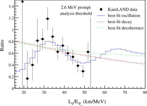
Figure 2: Ratio of the $\bar{\nu}_{e}$ reactor antineutrino flux measured by KamLAND to the expected flux without oscillations, as a function of $L/E$.

That KamLAND observes an energy-dependent suppression of the reactor $\bar{\nu}_{e}$ flux, just as predicted by fits of the oscillation model to solar neutrino data, is dramatic confirmation of the solar neutrino results and demonstrates that neutrino oscillation is the correct explanation of the flavour change of solar neutrinos observed by the SNO experiment.

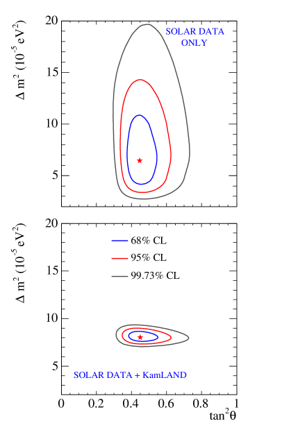
Figure 3: Oscillation parameter contours for solar neutrino data (top), and solar data + KamLAND data (bottom).

The solar experiments and KamLAND provide complementary constraints on the mixing parameters. Figure 3 demonstrates that solar neutrino experiments provide reasonably tight constraints on the mixing parameter $\tan^{2}\theta$, while the addition of KamLAND data sharply constrains the $\Delta m^{2}$ value.[7] This is because in the LMA region the solar neutrino survival probability determines the mixing angle through

$$|U_{e2}|^{2}\approx\sin^{2}\theta_{12}\approx\frac{\phi_{CC}}{\phi_{NC}}$$ (32)

while the observation of a distortion in the reactor antineutrino energy spectrum fixes $\Delta m_{21}^{2}$. Here the subscripts on $\theta_{12}$ and $\Delta m_{21}^{2}$ reflect the fact that solar neutrino oscillations involve the first and second mass eigenstates.

3.3 Atmospheric Neutrinos

Although the solar neutrino problem provided early indications that the Standard Model’s description of neutrinos is incomplete, resolution of the solar neutrino problem was a long time coming, and the first conclusive demonstration of neutrino oscillation actually came from studies of atmospheric neutrinos. Atmospheric neutrinos are produced when cosmic rays (primarily protons) collide in the upper atmosphere to make hadronic showers. These showers contain charged pions, which decay leptonically by $\pi^{\pm}\to\mu^{\pm}\nu_{\mu}$. The muons in turn generally decay in flight by $\mu^{\pm}\to e^{\pm}\nu_{\mu}\nu_{e}$, where I’ve ignored differences between $\nu$ and $\bar{\nu}$ states. A robust conclusion that follows from the decay sequence is that the ratio of $\nu_{\mu}$ to $\nu_{e}$ in the atmospheric neutrino flux should be 2:1.

In 1998 the Super-Kamiokande collaboration reported results showing that that ratio of the flux of $\nu_{\mu}$ to $\nu_{e}$ in fact is not 2:1, but is closer to 1:1.[5, 16] Closer examination revealed that while the $\nu_{e}$ flux in fact is in good agreement with Monte Carlo predictions, the $\nu_{\mu}$ flux shows a marked deficit. The size of this deficit varies with neutrino energy, and with the zenith angle of the event. This latter point is significant in that downgoing neutrinos are produced in the atmosphere just overhead, and have travelled $<10$ km before reaching Super-Kamiokande, while upgoing neutrinos are produced in the atmosphere on the far side of the Earth, and have travelled $\sim$13,000 km before reaching the detector.

Figure 4: Fluxes of atmospheric $\nu_{e}$ and $\nu_{\mu}$ as a function of zenith angle, as measured by Super-Kamiokande. The solid lines show the no oscillation prediction, while the dashed line passing through the data points is the best-fit oscillation prediction.

As seen in Figure 4, the deficit between the expected and measured number of $\nu_{\mu}$ is largest at low energy and at negative $\cos\theta$ (upward-going events).[17] This dependence on energy and on the distance travelled by the neutrino is characteristic of neutrino oscillations, and excludes a simple normalization error. These results were the first to establish conclusively that atmospheric neutrinos oscillate. The oscillation seems to be of the type $\nu_{\mu}\to\nu_{\tau}$. The atmospheric neutrino effect has been confirmed by a number of other experiments.[18]

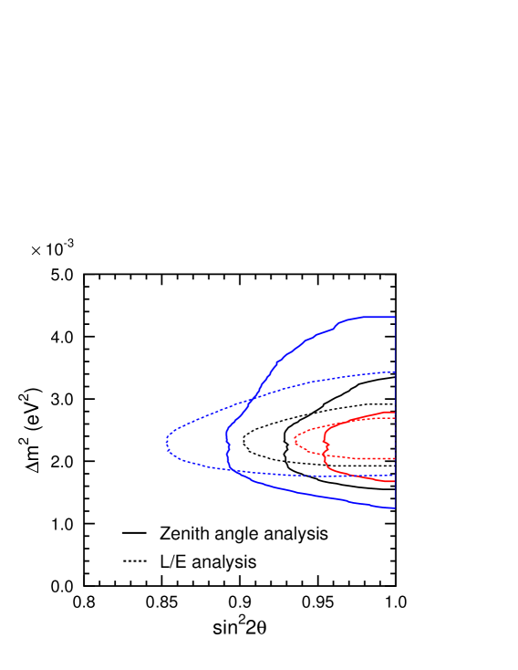
Figure 5: Super-Kamiokande atmospheric neutrino mixing contours. The two sets of contours are the 68%, 90%, and 99% contours from two different analysis techniques.

Figure 5 shows the inferred mixing parameters from fitting a two-flavour oscillation model to the atmospheric neutrino data.[16] The data favour $\Delta m^{2}\approx 2.5\times 10^{-3}$ eV² and, surprisingly, a maximal mixing angle of $\theta\approx 45^{\circ}$. (The term “maximal mixing” refers to the fact that each flavour eigenstate contains equal proportions of the two mass eigenstates if $\theta=45^{\circ}$.)

3.4 Long-Baseline Neutrino Oscillation Experiments

Just as solar neutrino oscillations have been confirmed with terrestrial (anti)-neutrinos by KamLAND, atmospheric neutrino oscillations have recently been confirmed by the K2K long-baseline neutrino oscillation experiment.[9] K2K produced a collimated beam of $\nu_{\mu}$ by colliding a 12 GeV proton beam with an aluminum target, thereby producing $\pi^{+}$’s. These pions were then collected and focused with a set of magnetic horns, and the collimated pion beam then decayed in a long evacuated decay pipe by $\pi^{+}\to\nu_{\mu}\mu^{+}$. The mean neutrino energy was 1.3 GeV, and the beam was aligned with the direction of the Super-Kamiokande detector, located 250 km away. A set of near neutrino detectors measured the neutrino beam’s energy spectrum, interaction, and relative cross sections at a point 300 m from the pion production target. By comparing the neutrino energy spectrum and rate at the near detector to those measured at Super-Kamiokande, the effects of neutrino oscillation over the 250 km baseline can be inferred. If the atmospheric neutrino effect is really explained by neutrino oscillations, then K2K should see an apparent “disappearance” of $\nu_{\mu}$, which oscillate into $\nu_{\tau}$ that are too low in energy to be detected in Super-K through charged current interactions.

Data collected by K2K between 1999 and 2004 in fact show a deficit of muon-like events, and some indication of an energy dependence to the $\nu_{\mu}$ disappearance effect as predicted for neutrino oscillations.[9] A combined maximum likelihood fit to the spectrum and rate excludes the null hypothesis of no oscillations at the 4.0$\sigma$ level. The best-fit oscillation parameters are $\Delta m^{2}=2.8\times 10^{-3}$ eV² and $\sin^{2}2\theta=1$, which are in excellent agreement with the values inferred from the atmospheric neutrino data.

The MINOS experiment is a conceptually similar long-baseline experiment in the United States. MINOS uses the NUMI neutrino beam produced by Fermilab’s Main Injector, with a far detector located $\sim 730$ km way in the Soudan mine in northern Minnesota, to study oscillations of $\nu_{\mu}$. MINOS should confirm K2K’s results with somewhat higher statistics, and at the time of writing results are expected imminently.

3.5 The Three-Flavour Picture

In the previous sections, the solar and atmospheric neutrino oscillation effects were each analyzed separately in terms of oscillations between two neutrino mass eigenstates. In reality, we know there are (at least) three flavour eigenstates, and so three mass eigenstates. Properly speaking we need to consider the 3$\times$3 MNS matrix, completely analogous to the CKM matrix for quarks, which can be parameterized as:

$$\begin{array}[]{lccc}U~{}=&\left(\begin{array}[]{ccc}1&0&0\\ 0&c_{23}&s_{23}\\ 0&-s_{23}&c_{23}\\ \end{array}\right)&\left(\begin{array}[]{ccc}c_{13}&~{}0{}&e^{i\delta}s_{13}\\ 0&1&0\\ -e^{-i\delta}s_{13}&0&c_{13}\\ \end{array}\right)&\left(\begin{array}[]{ccc}c_{12}&s_{12}&0\\ -s_{12}&c_{12}&0\\ 0&0&1\\ \end{array}\right)\end{array}$$ (33)

Here $c_{ij}\equiv\cos\theta_{ij}$ and $s_{ij}\equiv\sin\theta_{ij}$.

The $\theta_{12}$ term in this parameterization of the MNS matrix is that which controls solar neutrino oscillations, which involve the first and second mass eigenstates. Experimentally $\theta_{12}\approx 32^{\circ}$.[7] For comparison, the equivalent angle in the CKM matrix is the Cabibbo angle, which has the value $\theta_{C}\approx 13^{\circ}$. The mixing between the first and second generations of leptons is thus much larger than the mixing between the quark generations. Similarly, $\theta_{23}$, which determines the amplitude of atmospheric neutrino oscillations, is consistent with maximal mixing ($\theta_{23}\approx 45^{\circ}$), even though its quark counterpart equals just $\sim 2^{\circ}$! It is unknown at present by how much $\theta_{23}$ actually deviates from maximal mixing angle, or whether this value is indicative of some kind of flavour symmetry between the second and third generations.

By comparison, the middle part of Equation 33 is poorly constrained. Limits on oscillations of reactor neutrinos at short baselines ($\sim 1$ km) tell us that $\theta_{13}<9^{\circ}$.[4] In fact, current measurements of $\theta_{13}$ are consistent with zero. Presently nothing is known about the complex phase $\delta$ in the MNS matrix, which if non-zero would result in different oscillation patterns for neutrinos than for antineutrinos. This latter topic is of considerable interest. Recalling that all observed instances of CP violation in physics can be explained by a single complex phase in the CKM matrix, it is exciting to realize that the observation that neutrinos oscillate implies the possible existence of an entirely new source of CP violation—one involving leptons rather than quarks!

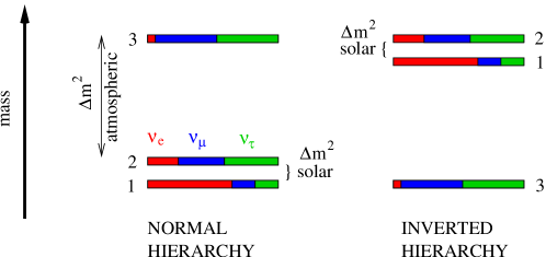
Figure 6: Normal and inverted neutrino mass hierarchies.

Measurements of atmospheric and solar neutrino oscillations also provide a partial determination of the pattern of the neutrino masses. Solar and reactor neutrino data have determined that $\Delta m^{2}_{21}\equiv m^{2}_{2}-m^{2}_{1}\approx 8.0\times 10^{-5}$ eV² (see Figure 3)[7], while atmospheric and long baseline neutrino experiments[16, 9] fix $|\Delta m_{32}^{2}|\approx 2.5\times 10^{-3}$ eV². The solar neutrino experiments have successfully inferred the sign of $\Delta m^{2}_{21}$ because the sign of the MSW effect in the Sun, which dominates in solar neutrino oscillations, depends on the sign of $\Delta m^{2}$. The atmospheric neutrino data however has no significant sensitivity at present to matter effects, and therefore it is not known whether $m_{2}<m_{3}$ or rather $m_{2}>m_{3}$. The result is that there are two possible mass hierarchies for the neutrino mass eigenstates. The so-called “normal” hierarchy has two light states and one heavier state, with $m_{1}<m_{2}<m_{3}$, while in the “inverted” hierarchy $m_{3}$ is the lightest state, with $m_{1}$ and $m_{2}$ being almost degenerate in mass (see Figure 6). Note that neutrino oscillation experiments are sensitive only to differences in $m^{2}$, and do not measure the absolute mass scale, although lower limits on the neutrino masses can be obtained by assuming the mass of the lightest mass eigenstate to be zero.

3.6 The LSND Result and the MiniBooNE Experiment

Until this point I have put off discussion of one other neutrino oscillation result that must be addressed. The LSND collaboration has reported 3.8$\sigma$ evidence for $\bar{\nu}_{\mu}\to\bar{\nu}_{e}$ oscillations of $\bar{\nu}_{\mu}$ produced from the decay of stopped $\mu^{+}$ in a beam dump, over a propagation distance of $\sim 30$ meters.[19] Other experiments, notably the KARMEN experiment, have failed to confirm this effect[20], but do not rule out the entire range of mixing parameters allowed by the LSND result. Mixing parameters with $\sin^{2}2\theta\approx 10^{-3}-10^{-2}$ and $\Delta m^{2}\sim 0.1-1$ eV² are consistent with all data.[21]

The inferred value of $\Delta m^{2}$ from the LSND result is much larger than those seen in solar and atmospheric neutrino experiments. If there are only three light neutrinos, then one can only form two independent mass differences $\Delta m^{2}$. If the LSND effect is due to neutrino oscillation, then it implies a third independent value of $\Delta m^{2}$, and so requires a fourth neutrino mass eigenstate. However, the LEP measurements of the $Z$ boson’s invisible decay width confirm that there are only three active light neutrinos.[22] A fourth light neutrino, if it exists, must be sterile! Even worse, more detailed analyses of solar and atmospheric neutrinos show no indication of any sterile neutrino admixtures, and are difficult to reconcile with the existence of a single sterile neutrino.[23] By adding more than one sterile flavour, enough wiggle room can be introduced to explain all of the oscillation results.

The LSND result presents a particular problem for neutrino physics. Because this result has not yet been confirmed by an independent experiment, and because it has relatively drastic consequences such as implying the existence of one or more sterile neutrino flavours, there is widespread skepticism regarding its correctness. That being said, no fundamental flaw in the LSND experiment has been demonstrated, and it is very possible that the result is correct. Neutrinos may then be more bizarre than anyone would have guessed! At present the MiniBooNE experiment at Fermilab is attempting to definitively check the LSND result[24], and is expected to produce first results for $\nu_{\mu}\to\nu_{e}$ oscillations sometime in 2006. Because the LSND result has not yet been confirmed and cannot easily be accommodated within the standard 3-flavour oscillation model, it is most often ignored. Only more data can determine whether it can be ignored without great peril.

4 Future Directions In Neutrino Oscillation

In less than a decade we have evolved from a situation in which we had no direct evidence that neutrinos oscillate to the present day, in which both $\Delta m^{2}$ parameters are known to $\sim$10-20%, and two of the three neutrino mixing angles are known at least approximately. One obvious way to proceed is to complete our picture of the MNS matrix by attempting to measure the unknown mixing parameters $\theta_{13}$ and $\delta_{CP}$, along with the sign of $\Delta m_{32}^{2}$ that determines whether neutrinos have a normal or inverted mass hierarchy.

4.1 Measuring $\theta_{13}$, The Mass Hierarchy, and CP Violation At Long-Baseline Experiments

The Super-K and K2K oscillation results seem to be of the type $\nu_{\mu}\to\nu_{\tau}$, and are well described by a two-flavour mixing model.[16, 9] However, in the full 3$\times$3 mixing picture, there should be some probability that $\nu_{\mu}$’s will instead oscillate into $\nu_{e}$’s in these experiments. For an $L/E$ value tuned to $\Delta m^{2}_{32}$, this probability is given by[25]:

$$P(\nu_{\mu}\to\nu_{e})\approx\sin^{2}2\theta_{13}\sin^{2}\theta_{23}\approx\frac{1}{2}\sin^{2}2\theta_{13}$$ (34)

Current limits on $\theta_{13}$ bound this probability to $<5\%$.

Because atmospheric neutrinos contain a significant fraction of $\nu_{e}$, observing the small $\nu_{\mu}\to\nu_{e}$ transition probability is not feasible. Long baseline experiments however can produce almost 100% pure beams of $\nu_{\mu}$. By searching for the appearance of a small $\nu_{e}$ component in the beam at the oscillation maximum, the value of $\theta_{13}$ may be inferred.

Equation 34 is only approximate, and the true $\nu_{e}$ appearance probability is modified by other mixing parameters and by matter effects. In particular, it can be shown that at the first oscillation maximum, the $\nu_{e}$ appearance probability in vacuum is altered in the presence of matter according to[26]:

$$P_{matter}(\nu_{\mu}\to\nu_{e})\approx\left(1+2\frac{E}{E_{R}}\right)P_{vacuum}(\nu_{\mu}\to\nu_{e})$$ (35)

where $E_{R}$ is a resonance energy given by $E_{R}=\Delta m_{32}^{2}/(2\sqrt{2}G_{F}N_{e})$. This matter effect depends on the number density of electrons $N_{e}$, and also on the magnitude and the sign of $\Delta m_{32}^{2}$. This matter effect correction is more significant at large $L$ or $E$ values, and has the opposite sign for neutrinos and antineutrinos.

A second confounding effect comes from the CP-violating phase of the MNS matrix. CP symmetry requires that neutrinos and antineutrinos oscillate identically, so that $P(\nu_{\mu}\to\nu_{e})=P(\bar{\nu}_{\mu}\to\bar{\nu}_{e})$ in vacuum. However, a non-zero value of $\delta_{CP}$ can make these probabilities unequal. One can then define a CP asymmetry for $\nu_{e}$ appearance which, ignoring matter effects, is given by[25]:

$$\mathcal{A}_{CP}=\displaystyle\frac{P(\nu_{\mu}\to\nu_{e})-P(\bar{\nu}_{\mu}\to\bar{\nu}_{e})}{P(\nu_{\mu}\to\nu_{e})+P(\bar{\nu}_{\mu}\to\bar{\nu}_{e})}\simeq\displaystyle\frac{\Delta m^{2}_{21}L}{4E_{\nu}}\cdot\frac{\sin 2\theta_{12}}{\sin\theta_{13}}\cdot\sin\delta_{CP}$$ (36)

The CP effect both changes $P(\nu_{\mu}\to\nu_{e})$ and creates a non-zero $\mathcal{A}_{CP}$. Notice that the size of $\mathcal{A}_{CP}$ as measured at the oscillation peak for the atmospheric neutrino $\Delta m_{32}^{2}$ depends on the solar neutrino parameters $\Delta m^{2}_{21}$ and $\theta_{12}$ as well. The reason for this is that, just as in the quark sector, CP violation in the neutrino sector is an interference effect: in this case, an interference between oscillations at the solar and atmospheric frequencies. To observe this effect, oscillations at both $\Delta m^{2}$ values must be of roughly comparable size, and $\theta_{13}$, which has the effect of coupling the atmospheric and solar oscillations in Equation 33, must be non-zero. Fortunately for those of us interested in actually observing CP violation by neutrinos, recent solar neutrino results establishing the LMA solution imply that both solar mixing parameters are reasonably large relative to the atmospheric neutrino mixing parameters. If $\theta_{13}$ is not too small, then observation of non-zero $\mathcal{A}_{CP}$ may be possible.

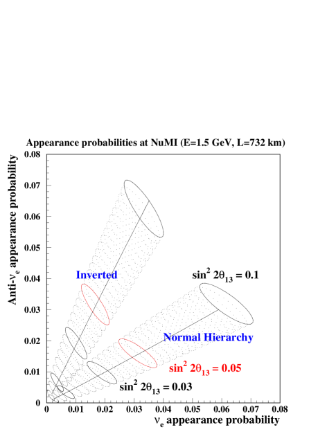
Figure 7: Oscillation probabilities for $\nu_{\mu}\to\nu_{e}$ vs. $\bar{\nu}_{\mu}\to\bar{\nu}_{e}$ for an off-axis experiment in the NUMI beamline. The solid diagonal lines correspond to $\delta_{CP}=0$.

Because the $\nu_{\mu}\to\nu_{e}$ oscillation probability depends on $\theta_{13}$, sign($\Delta m_{32}^{2}$), and $\delta_{CP}$, multiple measurements at different energies and/or baselines will be needed to disentangle the different effects. Figure 7 illustrates the dependence of $P(\nu_{\mu}\to\nu_{e})$ and $P(\bar{\nu}_{\mu}\to\bar{\nu}_{e})$ on the different oscillation parameters, for monoenergetic (anti)neutrino beams with $E=1.5$ GeV and $L=732$ km. The sign of $\Delta m_{32}^{2}$ defines the normal and inverted mass hierarchies, dividing the predicted probabilities into two separate “cones”. Increasing $\theta_{13}$ moves one out along either cone to larger oscillation probabilities. With $\theta_{13}$ and sign($\Delta m_{32}^{2}$) fixed, varying $\delta_{CP}$ traces out an ellipse in the plane, as shown in the figure. A suitably precise measurement of the neutrino and antineutrino appearance probabilities could determine the mass hierarchy for largish $\theta_{13}$, as well as defining an allowed region in the $\theta_{13}-\delta_{CP}$ plane. Measurements at different choices of $L$ and $E$ will have different sensitivity to matter effects and to $\delta_{CP}$ (see Equations 35 and 36), and can be used to break any remaining parameter degeneracies.

At present just one experiment to study $\nu_{e}$ appearance at the atmospheric $\Delta m^{2}$ has been funded. This is the T2K experiment in Japan.[25] T2K will use a megawatt-scale proton beam at the Japan Proton Accelerator Research Complex (JPARC) in Tokai to produce a $\nu_{\mu}$ beam that will be directed towards Super-Kamiokande, 295 km away. By pointing the neutrino beam about 2^∘ away from Super-K, T2K will take advantage of a trick called “off-axis focusing”, which results in a nearly monoenergetic neutrino beam with a peak energy of $\sim$700 MeV. At these energies the dominant interactions are charged current quasi-elastic ($\nu_{\ell}+n\to p+\ell$). A set of sophisticated near detectors will measure the beam properties before oscillation. T2K will have approximately 50 times greater statistics than K2K. With its relatively low beam energy and small baseline, T2K is relatively insensitive to matter effects.

The most important backgrounds to $\nu_{e}$ appearance at T2K are a small component of $\nu_{e}$ in the beam itself, and neutral current $\pi^{0}$ production at Super-K. The latter is only a background to $\nu_{e}$ appearance if Super-K fails to detect one of the two $\gamma$-rays. This could happen in very asymmetric decays in which one photon takes the bulk of the $\pi^{0}$’s energy, or if optical scattering of Cherenkov light sufficiently obscures one of the two Cherenkov rings. For five years of running at nominal luminosity ($5\times 10^{21}$ protons on target), T2K expects to achieve sensitivity to $\theta_{13}$ down to $\sin^{2}2\theta_{13}\approx 10^{-2}$ (the exact limit depends on the value of $\delta_{CP})$.[27] The measured value of $\theta_{13}$ is partially degenerate with $\delta_{CP}$, and separating the two parameters will require additional measurements with antineutrinos and/or at other baselines. Assuming that T2K successfully detects $\nu_{e}$ appearance in the $\nu_{\mu}$ beam, the natural followup is to switch the polarity of the beam and look for $\bar{\nu}_{\mu}\to\bar{\nu}_{e}$. With a beam power upgrade and possibly the construction of a larger far detector, this “phase 2” program could then begin to explore CP violation in the neutrino sector.

In addition to measuring the $\nu_{e}$ appearance probability, future long-baseline neutrino experiments such as T2K will measure the $\nu_{\mu}$ disappearance probability with much higher statistics, allowing precision measurements of $\Delta m_{32}^{2}$ and $\theta_{23}$. Such measurements can test how close $\theta_{23}$ is to maximal mixing ($45^{\circ}$), explore whether any fraction of the $\nu_{\mu}$ flux is oscillating to a non-interacting (sterile) neutrino flavour, and test the energy dependence of the neutrino oscillation prediction with high precision.

Although T2K is currently the only funded new long-baseline experiment to search for $\nu_{e}$ appearance, the NO$\nu$A collaboration in the US has proposed building a new off-axis detector, optimized for detecting electron appearance, in Fermilab’s NUMI beamline.[26] At a baseline of $\sim 730$ km and a beam energy of $\sim 2$ GeV, the NO$\nu$A experiment could have some sensitivity to matter effects and the sign of the mass hierarchy if $\theta_{13}$ is not too small, and would otherwise have similar sensitivity to $\nu_{e}$ appearance as T2K. The proposed far detector is a massive finely segmented liquid scintillator detector. The NO$\nu$A proposal is currently in the early stages of the approval process.

4.2 Reactor Neutrino Experiments

An alternate approach to measuring $\theta_{13}$ is to do precision reactor neutrino experiments at short baselines. The full 3-flavour formula for reactor $\bar{\nu}_{e}$ oscillation is[28]:

$$\begin{array}[]{ll}P(\bar{\nu}_{e}\to\bar{\nu}_{e})=1&-\sin^{2}2\theta_{13}\sin^{2}\left(\frac{1.27\Delta m_{13}^{2}L}{E}\right)\\ &-\cos^{4}\theta_{13}\sin^{2}2\theta_{12}\sin^{2}\left(\frac{1.27\Delta m_{21}^{2}L}{E}\right)\end{array}$$ (37)

The first term, which is proportional to $\sin^{2}2\theta_{13}$ and depends on the larger $\Delta m^{2}$ value, dominates over the second at short baselines. The second term only becomes significant at reactor neutrino energies for $L\approx 200$ km. KamLAND was successfully able to use the second term to confirm the solar neutrino effect[8], but experiments at shorter baselines instead yield limits on $\theta_{13}$. Currently the best limits on $\theta_{13}$ come from the CHOOZ reactor neutrino experiment, which limits $\sin^{2}2\theta_{13}<0.15$ at the 90% C.L.[4]

A new reactor neutrino experiment with high statistics and improved systematics may be able to achieve significantly improved $\theta_{13}$ sensitivity.[28] The keys to better sensitivity are to use a very intense reactor, with power in the gigawatt range, and to use both a near detector right next to the reactor and a far detector 1 or 2 km away in order to cancel systematics between the two detectors. A significant advantage of reactor $\theta_{13}$ experiments is that they are not sensitive to CP-violating effects (which can only be measured in an appearance measurement, not in a disappearance measurement), nor to matter effects, which are negligible at the relevant $L$ and $E$ values. A good reactor neutrino experiment therefore would provide a clean measurement of just $\theta_{13}$. This provides significant complementarity to long-baseline $\nu_{e}$ appearance experiments, which are sensitive to a combination of $\theta_{13}$, the mass hierarchy, and $\delta_{CP}$.

An added advantage of reactor $\theta_{13}$ experiments is that they are relatively inexpensive, with a typical estimated price tag of $\sim$$50M. For this reason, it seems that experimenters have proposed new experiments at virtually every reactor complex in the world with significant power output. Prominent sites for proposed experiments include Daya Bay in China, Braidwood in Illinois, and the Double CHOOZ proposal in France, although this list is far from exhaustive.[28] It seems likely that one or more of these proposals will be funded, but at present it is not clear which ones. The physics case for a sensitive reactor $\theta_{13}$ experiment seems compelling, however.

5 Altering The Standard Model To Accommodate Neutrino Mass

In the Standard Model, neutrinos have zero mass. This is not simply an ad hoc assumption, but a consequence of the fact that the Standard Model does not contain right-handed neutrino fields. Fermion mass terms in the Standard Model Lagrangian have the form $-m\bar{\psi}\psi=-m(\bar{\psi_{L}}\psi_{R}+\bar{\psi_{R}}\psi_{L})$. Without a right-handed field, no such term can exist. In this section I shall examine possible ways in which the Standard Model may be extended to include non-zero neutrino mass.

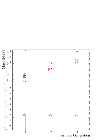
Figure 8: Masses of the Standard Model fermions. The purple lines indicate the range of allowed neutrino masses for $\nu_{1}$, $\nu_{2}$, and $\nu_{3}$, assuming a normal mass hierarchy.

The most obvious solution to this problem is to simply add right-handed neutrino states $\nu_{R}$ to the Standard Model and to give them Yukawa couplings to $\nu_{L}$ through the Higgs field, just like other fermions. This is called a Dirac mass term. While superficially this places neutrinos on the same footing as the other fermions, one striking difference is that $\nu_{R}$, having neither charge, colour, nor couplings to $W^{\pm}$ or $Z$, are sterile fields (i.e. they don’t couple to the vector gauge bosons)—making them in an important sense unlike all other Standard Model particles. An additional puzzle is that in order to explain the smallness of neutrino masses, their Yukawa couplings must be made anomalously small. As illustrated in Figure 8, within each generation the charged fermions are separated in mass by no more than 1 or 2 orders of magnitude, but the neutrino mass eigenstates are many orders of magnitude lighter than their charged counterparts. While it may rightfully be objected that we have no good explanations for the numerical values of the masses of any fermions, the disparity between neutrino and charged fermion masses suggests that neutrinos might not simply acquire mass in the same manner as other fermions.

Another possible way to add neutrino mass terms is to recognize that there already exists a right-handed neutral fermion in the Standard Model—namely, the antineutrino. Is it possible to identify $\nu_{R}$ with the antineutrino, and so generate mass terms of the form $\bar{\nu_{L}}\nu_{R}$ by combining a neutrino with its antineutrino? For charged fermions, the answer would clearly be no: since particles and antiparticles have opposite charges, a term that directly couples a fermion to its antifermion violates charge conservation! However, the situation is different with neutrinos, which are chargeless particles. The Majorana neutrino hypothesis takes advantage of this chargelessness by positing that an antineutrino is just a neutrino with its spin flipped by $180^{\circ}$! One might then form a “Majorana mass” term that couples a left-handed neutrino with the right-handed antiparticle.

Nonetheless, within the minimal Standard Model, Majorana mass terms are in fact forbidden. The reason is that although the Standard Model does not conserve either baryon number $B$ or lepton number $L$ non-perturbatively, it does conserve the quantity $B-L$ exactly. A Majorana mass term on the other hand results in $|\Delta(B-L)|=2$. It turns out that without extending the Standard Model particle content in some manner, a $B-L$ violating term cannot be generated at any order, even as an effective operator.[29]

However, the addition of an additional right-handed Majorana field to the Standard Model can resolve the problem. Let $\nu_{L}$ be a 2-component field describing left-handed neutrino/right-handed antineutrino that couples to weak interactions. Let $\nu_{R}$ now denote an additional right-handed Majorana field, independent of $\nu_{L}$, which does not couple to weak interactions. Because $\nu_{R}$ is an electroweak singlet, it can possess a bare Majorana mass term that couples $\nu_{R}$ to its antiparticle. We may also have a Dirac mass term (Yukawa coupling) between $\nu_{R}$ and the active light neutrino $\nu_{L}$. The mass terms in the Lagrangian are then[30, 29]:

$$-\Delta\mathcal{L}=m_{D}\bar{\nu_{L}}\nu_{R}+\frac{1}{2}m^{*}_{R}\nu_{R}^{T}C\nu_{R}+h.c.$$ (38)

The first term here is a Yukawa coupling between $\nu_{L}$ and $\nu_{R}$, and is referred to as a Dirac mass term. For charged fermions, this is the only allowed mass term. The second term is a Majorana mass term that couples $\nu_{R}$ to its antiparticle. This term is allowed, and violates no gauge symmetries, provided that $\nu_{R}$ is chargeless—that is, that $\nu_{R}$ is its own antiparticle. It’s evident that $\nu_{L}$ and $\nu_{R}$ should be thought of here as separate fields, with independent mass terms and in fact different masses.

Having written down Equation 38, some magic now results. We can rewrite the mass term in the Lagrangian as

$$-\Delta\mathcal{L}=\frac{1}{2}(\nu_{L},\nu_{R})\left(\begin{array}[]{cc}0&m_{D}\\ m_{D}&m_{R}\\ \end{array}\right)\left(\begin{array}[]{c}\nu_{L}\\ \nu_{R}\\ \end{array}\right)$$ (39)

Equation 39, which is not obviously diagonal, can be diagonalized to yield the physical mass eigenstates. There are two eigenvalues:

$$M_{heavy}\approx m_{R},\phantom{XXXXXXXX}M_{light}\approx\frac{m^{2}_{D}}{m_{R}}$$ (40)

Because $\nu_{R}$ is an electroweak singlet, its mass is not protected by any electroweak symmetry, and the theoretical expectation is that it should be quite massive—possibly at the GUT scale.[29, 30] On the other hand, we would naively expect $m_{D}$ to be similar in size to the Dirac masses of other fermions. If we take $m_{R}=10^{15}$ GeV as a typical GUT-scale energy and $m_{D}=200$ GeV as representative of the Yukawa coupling of the heaviest charged fermion, we would estimate the largest light neutrino mass to be $M_{light}=(200~{}{\rm GeV})^{2}/(10^{15}~{}{\rm GeV})=0.04$ eV. This value is exactly the right order of magnitude for the neutrino mass inferred by $\sqrt{\Delta m^{2}_{32}}\approx 0.05$ eV!

Something semi-miraculous has occurred. By introducing a right-handed neutrino with a mass near the GUT scale, as is motivated by GUT models, with a “normal” Dirac coupling $m_{D}$ to $\nu_{L}$, we naturally produce very light neutrino masses for $\nu_{L}$, without having to fine-tune the Dirac mass coupling. The heavier that $M_{heavy}$ is, the lighter that $M_{light}$ becomes, which gives rise to the name “seesaw mechanism” for this method of generating light neutrino masses. Obviously the close numerical correspondence between $\sqrt{\Delta m_{32}^{2}}$ and $M_{light}$ in the previous paragraph should not be taken too seriously, since we do not know the exact values of $m_{R}$ or $m_{D}$ to use in the calculation. The exact mass calculation in fact depends on the details of the physics at higher energy scales. Nonetheless, the seesaw mechanism provides as least a proof of principle as to how very light neutrino masses can be generated without fine-tuning the Dirac mass coupling, while providing a fascinating example of a novel method of generating masses for fundamental particles.

6 Determining The Absolute Mass Scale Of Neutrinos

Although neutrino oscillation measurements demonstrate the existence of neutrino masses, they cannot determine the absolute values of the masses, since oscillations are only sensitive to differences in $\Delta m^{2}$. One may make an educated guess of the absolute masses if one assumes that each mass eigenstate is much heavier than the previous one ($m_{1}\ll m_{2}\ll m_{3}$), reproducing the pattern of charged fermion masses. In this limit then $m_{1}\approx 0$ eV, $m_{2}\approx\sqrt{\Delta m_{21}^{2}}=0.009$ eV, and $m_{3}\approx\sqrt{\Delta m_{32}^{2}}=0.05$ eV. For an inverted hierarchy we get $m_{3}\approx 0$ eV and $m_{1}\approx m_{2}\approx 0.05$ eV.

Of course it is not clear whether a strict mass hierarchy should hold. As the mass of the lightest mass eigenstate increases, the three mass eigenstates approach a limit of degenerate masses. The best upper limits on neutrino mass come from cosmology. Massive neutrinos act as a form of hot dark matter that tends to wash out clustering at small angular scales during structure formation, since relativistic dark tends to “stream out” of small density perturbations, but not larger ones. This effect can leave signatures in the cosmic microwave background radiation, in weak lensing surveys, and in large scale structure surveys. While the exact limits obtained depend on which data sets are included in the fits and with what priors, the published limits[31] for the sum of the three mass eigenstates range from $\sim 0.4-0.7$ eV. It would not be far wrong to say that cosmology limits the mass of any individual mass eigenstate to be $<0.2$ eV.

Less stringent but more model-independent limits come from measurements of the energies of the products of weak decays. Notable among these are studies of the endpoint of tritium beta decay. If neutrinos have non-zero mass, this mass has the effect of reducing the maximum energy available for the $\beta$ particle in the decay. Careful measurements of the shape of the $\beta$ energy spectrum at the endpoint limit the effective mass of a $\nu_{e}$ (the weighted average of its mass eigenstates) to $<2.5$ eV at the 95% C.L. The KATRIN collaboration has proposed a next generation tritium endpoint measurement with sensitivity down to 0.2 eV, which might be able to measure or rule out the case of three quasi-degenerate masses.[32]

6.1 Neutrinoless Double Beta Decay

In a class by themselves are experiments to measure neutrinoless double beta decay. Normal double beta decay is a doubly weak process in which a nucleus decays by simultaneously emitting two electrons and two $\bar{\nu}_{e}$. Double beta decay can occur when single beta decay is energetically forbidden, but the $|\Delta Z|=2$ process is energetically allowed. If neutrinos are Majorana particles (so that a neutrino is its own antiparticle), then instead of emitting two neutrinos, a Feynman diagram exists in which a virtual neutrino is emitted then reabsorbed as an antineutrino. The result is a beta decay in which two electrons but no neutrinos are emitted. Neutrinoless double beta decay violates lepton number by $|\Delta L|=2$, and differs kinematically from ordinary double beta decay in that the two emitted electrons now contain all of the emitted energy of the transition. The experimental signature of neutrinoless double beta decay is therefore a peak right at the endpoint of the distribution of the sum of the two electrons’ energies.

The rate of neutrinoless double beta decay depends on the available phase space and on nuclear matrix elements of the decaying nucleus, but can also be shown to depend an effective neutrino mass by[30]:

$$R\propto\langle m_{\nu}\rangle^{2}=\left|\sum_{i}^{N}U_{ei}^{2}m_{i}\right|^{2}$$ (41)

The effective mass depends on the elements in the first row of the MNS matrix. The mass values enter because they control how much of the “wrong” chirality is mixed into each neutrino, determining the transition of a Majorana neutrino into an antineutrino. (Recall that by the Majorana neutrino hypothesis an antineutrino is just a neutrino of the opposite chirality.)

Positive detection of neutrinoless double beta decay would arguably be the most exciting possible result in neutrino physics, since it would simultaneously establish that neutrinos are Majorana particles, show that lepton number is violated, and settle what the absolute values of the neutrino masses are. This phenomenon has been searched for in many candidate nuclei, but no confirmed detections have been found. The best upper limits comes from the ⁷⁶Ge system, which limits $\langle m_{\nu}\rangle<0.35$ eV at the 90% C.L.[33]

While neutrinoless double beta decay experiments are tremendously difficult due to the rarity of such decays and the existence of various potential backgrounds, many proposals for next generation experiments exist. These proposals rely on much larger exposures (kilograms of material $\times$ years of data-taking), and on sophisticated active or passive means to reject backgrounds. One such proposed experiment is the MAJORANA experiment, whose goal is to collect 2500 kg-years exposure of ⁷⁶Ge to achieve sensitivity down to $\langle m_{\nu}\rangle<0.05$ eV.[34] The EXO experiment will look for neutrinoless double beta decay in 10 tonnes of ¹³⁶Xe in a liquid or gas TPC, and will attempt to tag the resulting barium ion using spectroscopic techniques to eliminate backgrounds, with a sensitivity goal of $\sim 0.01$ eV.[35] These and other next-generation experiments, if successful, have some hope of covering the expected range for $\langle m_{\nu}\rangle$ for degenerate neutrino masses and for the inverted hierarchy. A null result would tell us that neutrinos, if Majorana particles, must have a normal mass hierarchy, but by itself could not distinguish between the possibilities that neutrinos either have a normal mass hierarchy or are simply not Majorana particles. (In principle, though, a determination from long baseline neutrino oscillation experiments that neutrinos have an inverted mass hierarchy, combined with a null result from a sufficiently sensitive neutrinoless double beta decay experiment, could demonstrate that neutrinos are not Majorana particles!)

7 Conclusions

The past decade of neutrino physics has been revolutionary. We have gone from having no confirmed evidence for neutrino physics beyond the Standard Model to the current situation, in which oscillation has been observed in four separate systems, with reasonably precise measurements of two $\Delta m^{2}$ values and two of the four independent mixing parameters in the MNS matrix (assuming that this matrix really is unitary!) Neutrino oscillation is new physics beyond the Standard Model, and requires the addition of new fields and new parameters to the Standard Model. It may even point to the existence of new mechanisms of mass generation.

With the discovery of neutrino mixing, we are now entering an era of precision lepton flavour physics. Just as the study of the CKM matrix has been one of the most important areas in particle physics for decades, studies of lepton flavour may lead to new insights into the origins of flavour, CP violation, and the relationship between quarks and leptons.

In the near future, the experimental emphasis is likely to be on determining $\theta_{13}$ through long baseline or reactor neutrino experiments, as well as precisely testing the predictions of the neutrino oscillation model. Longer term we can aspire to looking for CP violation by neutrinos in long baseline oscillation experiments, searching for neutrinoless double beta decay in an attempt to answer the Majorana vs. Dirac neutrino question, and improving limits on neutrino mass from direct kinematic experiments or from cosmology. All the while anomalies like the controversial LSND result remind us that neutrinos may present other surprises that we have not even anticipated yet.

Clearly I’m an optimist about the future of neutrino research. Given that neutrino oscillations are the first new particle physics beyond the Standard Model, the (over?)abundance of new proposals for experiments, and the fact that even today neutrino experiments are probing new physics at a tiny fraction of the cost of large collider experiments, how can I not be an optimist for the future of our field? I hope in the end that the reader agrees with me in this regard.

References

- [1] Z. Maki, N. Nakagawa, and S. Sakata, Prog. Theor. Phys. 28, 870 (1962); V. Gribov and B. Pontecorvo, Phys. Lett. B28 493 (1969).
- [2] Danby et al., PRL 9, 36 (1962).
- [3] S. P. Mikheyev and A. Yu. Smirnov, Sov. J. Nucl. Phys. 42 913 (1985); L. Wolfenstein, Phys. Rev. D17 2369 (1978).
- [4] M. Apollonio et al., Eur. Phys. J. C27, pp. 331-374 (2003).
- [5] Y. Fukuda et al., PRL 81 (1999) 1562-1567; Y. Fukuda et al., PRL 82 (1999) 2644-2648.
- [6] Q. R. Ahmad et al., PRL 87 (2001) 071301; Q. R. Ahmad et al., PRL 89 (2002) 011301; Q. R. Ahmad et al., PRL 87 (2001) 011302; S. N. Ahmed et al., PRL 92 (2004), 181301.
- [7] B. Aharmin et al., Phys. Rev. C72 (2005), 055502.
- [8] T. Araki et al., PRL 94 (2005) 081801; K. Eguchi et al., PRL 90 (2003) 021802.
- [9] E. Aliu et al., PRL 94 (2005), 081802; M. H. Ahn et al., PRL 90 (2003), 041801.
- [10] John Bahcall, Neutrino Astrophysics, Cambridge University Press, 1989.
- [11] B. T. Cleveland et al., Astrophys. J. 496, 505 (1998).
- [12] See for example Bahcall et al., Astrophys. J. 621 (2005) L85-L88.
- [13] J. Hosaka et al., hep-ex/0508053, submitted to PRD; M. B. Smy et al., Phys. Rev D69 (2004) 011104; S. Fukuda et al., Phys. Lett. B539, 179 (2002).
- [14] V. Gavrin, Results from the Russian American Gallium Experiment (SAGE), VIIIth International Conference on Topics in Astroparticle and Underground Physics (TAUP 2003), Seattle, September 5–9, 2003; J.N. Abdurashitov et al., J. Exp. Theor. Phys. 95, 181 (2002); C. Cattadori, Results from Radiochemical Solar Neutrino Experiments, XXIst International Conference on Neutrino Physics and Astrophysics (Neutrino 2004), Paris, June 14–19, 2004.; E. Bellotti, The Gallium Neutrino Observatory (GNO), VIIIth International Conference on Topics in Astroparticle and Underground Physics (TAUP 2003), Seattle, September 5–9, 2003; M. Altmann et al., Phys. Lett. B 490, 16 (2000); W. Hampel et al., Phys. Lett. B 447, 127 (1999).
- [15] SNO Collaboration, Nucl. Instr. and Meth. A449 (2000), 1972.
- [16] Y. Ashie et al., Phys.Rev. D71 (2005) 112005; Y. Ashie et al., PRL 93 (2004) 101801.
- [17] M. Ishitsuka, Proceedings for the XXXIXth Recontres de Moriond on Electroweak Interactions (2004), hep-ex/0406076.
- [18] For example, see M. Ambrosio et al., Eur. Phys. J. C35 (2004), 323; M. Sanchez et al., Phys. Rev. D68 (2003), 113004; K.S. Hirata et al., Phys. Lett. B280, 146 (1992).
- [19] A. Aguilar et al., Phys. Rev. D64 (2001) 112007.
- [20] B. Armbruster et al., Phys. Rev. D65 (2002) 112001.
- [21] Church et al., Phys. Rev. D66 (2002) 013001.
- [22] ALEPH, DELPHI, L3, OPAL, and SLD Collaborations, accepted for publication in Physics Reports, CERN-PH-EP/2005-051, SLAC-R-774, hep-ex/0509008.
- [23] M. Maltoni et al., Nucl. Phys. B 643 (2002) 321.
- [24] H. Ray, Int. J. Mod. Phys. A20 (2005) 3062; M. H. Shaevitz, prepared for the Fujihara Seminar: Neutrino Mass and the Seesaw Mechanism, KEK, Japan, February, 2004, hep-ex/0407027.
- [25] Y. Itow et al., “The JHF-Kamioka neutrino project”, hep-ex/0106019
- [26] D. Ayres et al., “Letter of Intent to build an Off-axis Detector to study oscillations with the NUMI Neutrino Beam, hep-ex/0210005.
- [27] T2K Collaboration, “T2K ND280 Conceptual Design Report”, T2K Internal Document
- [28] K. Anderson et al., “White Paper Report on Using Nuclear Reactors to Serach for a value of ”, January 2004, hep-ex/0402041.
- [29] For a good general discussion of neutrino masses, see E. Kh. Akhmedov, “Neutrino Physics”, Lectures given at the Trieste Summer School in Particle Physics, June 7-July 9, 1999, hep-ph/0001264.
- [30] S. R. Elliott & P. Vogl, Ann. Rev. Nucl. Part. Sci 52 (2002), 115-151.
- [31] See for example O. Elgaroy & O. Lahav, New. J. Phys. 7 (2005), 61.
- [32] KATRIN collaboration, “KATRIN: A next generation tritium beta decay experiment with sub-eV sensitivity for the electron neutrino mass” (2001), hep-ex/0109033.
- [33] H.V. Klapdor-Kleingrothaus et al., Eur. Phys. J. A12 (2001), 147; C. E. Alseth et al,. Phys. Rev. C 59 (1999), 2108; C. .E. Alseth, Phys. Rev. D 75 (2002), 092007.
- [34] Majorana collaboration, “White Paper on the Majorana Zero-Neutrino Double-Beta Decay Experiment” (2003), http://majorana.pnl.gov/documents/WhitePaper.pdf
- [35] M. Danilov et al., Phys. Lett. B 480 (2000), 12-18.