Multivariate searches for single top quark production with the DØ detector

Abstract

We present a search for electroweak production of single top quarks in the $s$-channel (${\mbox{$p\bar{p}$}}{\mbox{$\rightarrow$}}t\bar{b}$+$X$) and $t$-channel (${\mbox{$p\bar{p}$}}{\mbox{$\rightarrow$}}tq\bar{b}$+$X$) modes. We have analyzed 230 pb^-1 of data collected with the DØ detector at the Fermilab Tevatron collider at a center-of-mass energy of $\sqrt{s}=1.96$ TeV. Two separate analysis methods are used: neural networks and a cut-based analysis. No evidence for a single top quark signal is found. We set 95% confidence level upper limits on the production cross sections using Bayesian statistics, based on event counts and binned likelihoods formed from the neural network output. The limits from the neural network (cut-based) analysis are 6.4 pb (10.6 pb) in the $s$-channel and 5.0 pb (11.3 pb) in the $t$-channel.

I Introduction

The top quark, discovered in 1995 at the Fermilab Tevatron Collider by the CDF and DØ collaborations topdiscovery , is by far the heaviest elementary particle found to date. Its large mass and corresponding coupling strength to the Higgs boson of order unity suggest that the physics of electroweak symmetry breaking might be visible in the top quark sector.

Top quarks are produced at the Tevatron mainly in top-antitop pairs through the strong interaction. This mode led to the discovery of the top quark and has been the only top quark production mode observed to date. The top quark decays predominantly to a $W$ boson and a $b$ quark, but little else is known experimentally about its electroweak interactions.

All previous studies of the top quark electroweak interaction and the $Wtb$ vertex have been done either in the low-energy regime using virtual top quarks (in studies of $b$ quark decays), or in the decay of real top quarks. Both of these types of studies presuppose the unitarity of the CKM matrix and are thus constrained to studying the standard model with three generations of quarks. This restriction can be overcome by exploring the production of single top quarks through electroweak interactions. This production mode is becoming accessible at the Tevatron and promises the first direct measurement of the electroweak coupling strength of the top quark as well as a first glimpse at possible top quark interactions beyond the standard model (SM).

I.1 Physics with Single Top Quarks

The study of single top quark production provides the possibility of investigating top quark related properties that cannot be measured in top quark pair production. The most relevant of these is a direct measurement of the CKM matrix element $|V_{tb}|$ from the single top quark production cross sections. This provides the only measurement of $|V_{tb}|$ without having to assume three quark generations or CKM matrix unitarity. Together with the other CKM matrix measurements Hagiwara:fs , we will be able to test the unitarity of the CKM matrix.

Single top quarks are produced through a left-handed interaction. Therefore, they are expected to be highly polarized. Since the top quark decays before hadronization can occur, the spin correlations are retained in the final decay products. Hence, single top quark production offers an opportunity to observe the polarization and to test the corresponding SM predictions.

Measurements of the charged-current couplings of the top quark probe any nonstandard structure of the couplings and can therefore provide hints of new physics. Any deviation in the $(V$–$A)$ structure of the $Wtb$ coupling would lead to a violation of the spin correlation properties Heinson:1996zm . Furthermore, combining single top quark measurements with $W$ helicity measurements in top quark decays provides the most stringent information on the $Wtb$ coupling Chen:2005vr .

Finally, rather than manifesting itself in a modified $Wtb$ coupling, new physics could produce a single top quark final state through other processes. There are several models of new physics that would increase the single top quark production cross sections Tait:2000sh . Thus, constraints on physics beyond the standard model are possible even before an actual observation of single top quark production.

I.2 Single Top Quark Production

There are three standard model modes of single top quark production at hadron colliders. Each of these modes may be characterized by the four-momentum squared $Q^{2}_{W}$, the virtuality, of the participating $W$ boson:

• $s$-channel $W$ boson exchange ($Q^{2}_{W}>0$): This process, ${\mbox{$p\bar{p}$}}{\mbox{$\rightarrow$}}t\bar{b}$+$X$, is referred to as “$tb$,” which includes both $t\bar{b}$ and $\bar{t}b$ (see Fig. 1).

• $t$-channel and $u$-channel $W$ boson exchange ($Q^{2}_{W}<0$): This process, ${\mbox{$p\bar{p}$}}{\mbox{$\rightarrow$}}tq\bar{b}$+$X$, has the largest cross section of the three. It includes the leading order diagram (Fig. 2a) with a $b$ quark from the proton sea in the initial state, and a second diagram (Fig. 2b) where an extra $\bar{b}$ quark appears in the final state explicitly. This latter mode is of order $O(\alpha_{s})$ in the strong coupling $\alpha_{s}$, but nevertheless provides the largest contribution to the total cross section. Historically, $t$-channel production has also been referred to as $W$-gluon fusion, since the $\bar{b}$ quark in the final state arises from a gluon splitting to a $b\bar{b}$ pair. We refer to the $t$-channel process as “$tqb$,” which includes $tq\bar{b}$, $\bar{t}\bar{q}b$, $tq$, and $\bar{t}\bar{q}$.

• Real $W$ boson production ($Q^{2}_{W}=m_{W}^{2}$): In this process, $p\bar{p}\to tW$+$X$, a single top quark appears in association with a real $W$ boson in the final state. This process has a negligible cross section at the Tevatron Heinson:1996zm and will not be addressed in this paper.

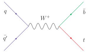
Figure 1: Feynman diagram for leading order $s$-channel single top quark production.

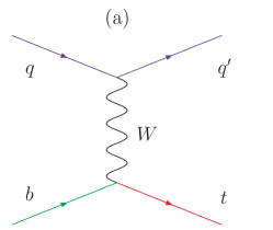
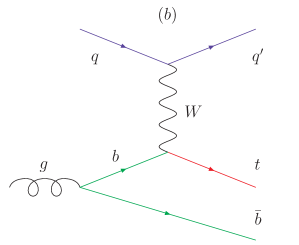
Figure 2: Representative Feynman diagrams for $t$-channel single top quark production. Shown is the (a) leading order and (b) the $O(\alpha_{s})$ $W$-gluon fusion diagram.

The next-to-leading order (NLO) production rates at the Tevatron ($\sqrt{s}=1.96$ TeV) for the $s$- and $t$-channel single top quark modes have been calculated Smith:1996ij ; Stelzer:1997ns ; Harris:2002md ; sintop-xsec2 ; Campbell:2004ch ; sintop-nlo-sch ; sintop-nlo-tch and the results for cross sections are shown in Table 1. The uncertainties include components from the choice of scale and the parton distribution functions, but not for the top quark mass.

Table 1: Theoretically calculated total cross sections for single top quark production at a $p\bar{p}$ collider with $\sqrt{s}=1.96$ TeV, using $m_{t}=175$ GeV.

Process	Cross Section [pb]
$s$-channel ($tb$)	$0.88^{+0.07}_{-0.06}$
$t$-channel ($tqb$)	$1.98^{+0.23}_{-0.18}$
$tW$ production	$0.093\pm 0.024$

For comparison, the calculated top quark pair production cross section at the Tevatron at 1.96 TeV is $6.77\pm 0.42$ pb Kidonakis:2003qe . This already makes it clear that it is more difficult to isolate the single top quark signal than the top quark pair signal.

Under the assumption that all top quarks decay to a $W$ boson and a $b$ quark, and only using $W$ boson decays to electron and muon final states, the final state signature of a single top quark event detected in this analysis is characterized by a high transverse momentum ($p_{T}$), centrally produced, isolated lepton ($e^{\pm}$ or $\mu^{\pm})$ and missing transverse energy ($\not\!\!E_{T}$), together with two or three jets. One of the jets comes from a high-$p_{T}$ central $b$ quark from the top quark decay.

Figures 3 and 4 shows the transverse momenta and pseudorapidities $\eta$ fiducial_endnote for the partons in our modeling of the $s$-channel and $t$-channel single top quark processes, after decay of the top quark and $W$ boson.

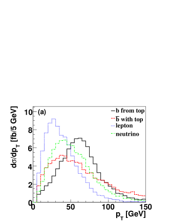
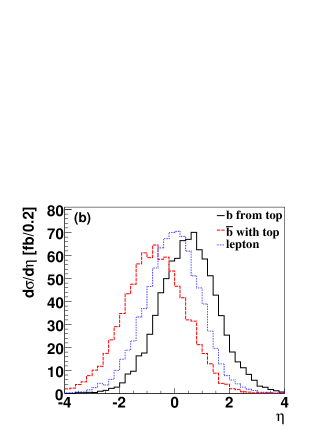
Figure 3: Distributions of transverse momenta (a) and pseudorapidity (b) for the final state partons in $s$-channel single top quark events. The histograms only include the final state of $t$, not $\bar{t}$.

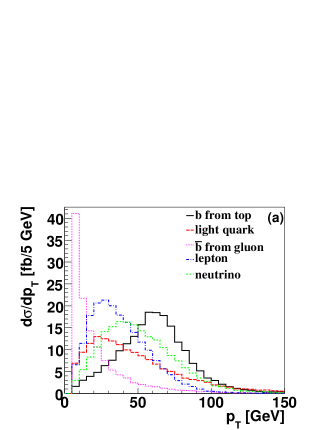
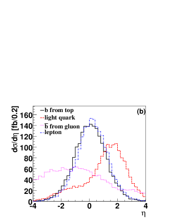
Figure 4: Distributions of transverse momenta (a) and pseudorapidity (b) for the final state partons in $t$-channel single top quark events. The histograms only include the final state of $t$, not $\bar{t}$.

The final state fermions from the top quark decay have relatively high transverse momenta and central rapidities. Since the $s$-channel process involves the decay of a heavy virtual object, the $\bar{b}$ quark produced with the top quark is also at high transverse momentum and central pseudorapidity. By contrast, the light quark in the $t$-channel appears at lower transverse momentum and at more forward pseudorapidities because it is produced when an initial state parton emits a virtual $W$ boson. The $\bar{b}$ quark from $t$-channel initial state radiation appears typically at very low $p_{T}$ and with large pseudorapidities and is thus often not reconstructed experimentally.

Due to its electroweak nature, single top quark production results in a polarized final state top quark. It has been shown Mahlon:1995zn that the top quark spin follows the direction of the down-type quark momentum in the top quark rest frame. This is the direction of the initial $\bar{d}$ quark for the $s$-channel and close to the direction of the final state $d$ quark for the $t$-channel. The above result follows directly from the properties of the polarized top quark decays when single top quark production is considered as top quark decay going “backwards in time” Boos:2002xw .

I.3 Overview of the Backgrounds

Searches for single top quark production are challenging because of the very large backgrounds. The situation is significantly different from top pair production not just because of the smaller production rate, but more importantly because of the smaller multiplicity of final state particles (leptons or jets). Single top quark events are typically less energetic (because there is only one heavy object), less spherical (because of the production mechanism), and typically have two or three jets, not four as do $t\bar{t}$ events.

Processes that can have the same single top quark experimental signature include in order of importance $W$+jets, $t\bar{t}$, multijet production, and some smaller contributions from $Z$+jets and diboson events.

• $W$+jets events form the dominant part of the background. The cross section for $W$+2 jets production is over 1000 pb Mangano:2002ea ; Mrenna:2003if with $W{\mbox{$b\bar{b}$}}$ contributing about 1%.

• The second largest background is due to $t\bar{t}$ production. This process has a larger multiplicity of final state particles than single top quark events. However, when some of the jets or a lepton are not identified, the kinematics of the remaining particles are very similar to those of the signal.

• Multijet events form a background in the electron channel when a jet is misidentified as an electron. The probability of such misidentification is rather small, but the $\geq$3 jet cross section is so large that the overall contribution is significant.

  Additionally, $b\bar{b}$ production contributes to the background when one of the $b$’s decays semileptonically. This background in the electron channel is very small. In the muon channel, $b\bar{b}$ events form a background when the muon is away from the jet axis or when the jet is not reconstructed.

• $Z$/Drell-Yan+jets production can mimic the single top quark signals if one of the leptons is misidentifed.

• $WW$, $WZ$, and $ZZ$ processes are the electroweak part of the $W$+jets and $Z$+jets backgrounds, but with different kinematics.

Single top quark events are kinematically and topologically similar to $W$+jets and $t\bar{t}$ events. Therefore, extracting the signal from the backgrounds is challenging in a search for single top quark production.

I.4 Status of Searches

Both the CDF and DØ collaborations have previously performed searches for single top quark production d0runI ; Acosta:2001un . Recently, CDF performed a search using 160 pb^-1 of data and obtained upper limits of 13.6 pb ($s$-channel), 10.1 pb ($t$-channel), and 17.8 pb ($s$+$t$ combined) at the 95% confidence level RunII:cdf_result . DØ has published a neural network search for single top quark production using 230 pb^-1 of data RunII:d0_result , which is described in more detail in this article.

I.5 Outline of the Analysis

We have performed a search for the electroweak production of single top quarks in the $s$-channel and $t$-channel production modes with the DØ detector at the Fermilab Tevatron collider. We consider lepton+jets in the final state, where the lepton is either an electron or a muon.

To take advantage of the differences between $s$- and $t$-channel final state topologies, we differentiate the $s$-channel search from the $t$-channel search by requiring at least one untagged jet in the $t$-channel search. For both $s$-channel and $t$-channel searches, we separate the data into independent analysis sets based on the lepton flavor ($e$ or $\mu$) and the multiplicity of identified $b$ quarks (one tagged jet or more than one).

We use two different multivariate methods to extract the signal from the large backgrounds: a cut-based analysis, first presented here, and an analysis based on neural networks that was first presented in brief form in Ref. RunII:d0_result . In the absence of any significant evidence for signal, we set upper limits at the 95$\%$ C.L. on the single top quark production cross sections.

Finally, we present limit contours in a two-dimensional plane of the $s$-channel signal cross section versus the $t$-channel signal cross section.

I.6 Outline of the Paper

This paper is organized as follows. Section II describes the DØ detector and the reconstruction of the final state objects. Section III summarizes the triggers for the data samples used in the search and Section IV describes the selection requirements. Section V explains the modeling of signals and backgrounds, and Section VI presents the numbers of events passing all selections. Section VII discusses the most important variables that offer discrimination between the signals and backgrounds, and provides details of the cut-based and the neural network analyses. Section VIII lists the systematic uncertainties in this measurement. Section IX discusses the procedure for setting limits on the signal cross section using Bayesian statistics. The limits are presented in Section X, and we summarize the results in Section XI.

II The DØ Detector and Object Reconstruction

II.1 The DØ Detector

The DØ detector Abazov:2005pn is shown in Figs. 5 and 6 and consists of several layered elements. The first is a magnetic central-tracking system, which includes a silicon microstrip tracker (SMT) and a central fiber tracker (CFT), both located within a 2 T superconducting solenoidal magnet. The SMT has $\approx 800,000$ individual strips, with a typical pitch of $50-80$ $\mu$m, and a design optimized for tracking and vertexing capability at pseudorapidities of $|\eta|<3.0$. The system has a six-barrel longitudinal structure, each with a set of four layers arranged axially around the beam pipe, and interspersed with 16 radial disks. The CFT has eight thin coaxial barrels, each supporting two doublets of overlapping scintillating fibers of 0.835 mm diameter, one doublet being parallel to the collision axis, and the other alternating by $\pm 3^{\circ}$ relative to the axis. Light signals are transferred via clear light fibers to solid-state photon counters (visible light photon counters, VLPCs) that have $\approx 80\%$ quantum efficiency.

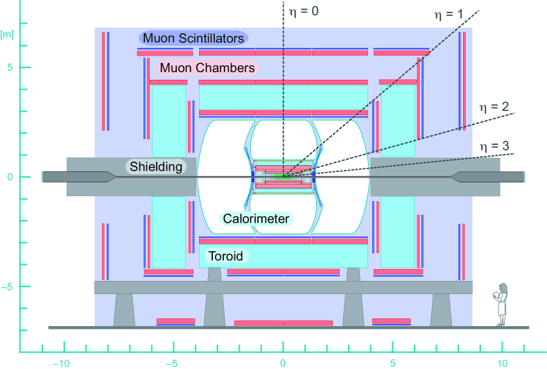
Figure 5: General view of the DØ detector. The proton beam travels from left to right and the antiproton beam from right to left in this figure.

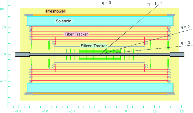
Figure 6: Close view of the tracking systems.

Central and forward preshower detectors are located just outside of the superconducting coil (in front of the calorimetry). These are constructed of several layers of extruded triangular scintillator strips that are read out using wavelength-shifting fibers and VLPCs. The next layer of detection involves three liquid-argon/uranium calorimeters: a central section (CC) covering $|\eta|$ up to $\approx 1$, and two end calorimeters (EC) extending coverage to $|\eta|\approx 4$, all housed in separate cryostats run1det . In addition to the preshower detectors, scintillators between the CC and EC cryostats provide sampling of developing showers for $1.1<|\eta|<1.4$.

A muon system resides beyond the calorimetry, and consists of a layer of tracking detectors and scintillation trigger counters before 1.8 T iron toroids, followed by two more similar layers after the toroids. Tracking for $|\eta|<1$ relies on 10 cm wide drift tubes run1det , while 1 cm mini drift tubes are used for $1<|\eta|<2$.

The luminosity is obtained from the rate of inelastic collisions measured using plastic scintillator arrays located in front of the EC cryostats, covering $2.7<|\eta|<4.4$.

II.2 Object Reconstruction

Physics objects are reconstructed from the digital signals recorded in each part of the detector. Particles can be identified by certain patterns and, when correlated with other objects in the same event, they provide the basis for understanding the physics that produced such signatures in the detector.

II.2.1 Primary Vertex

The position of the hard scatter interaction is determined at DØ by clustering tracks into seed vertices using a Kalman filter algorithm kalman . The primary vertex is then selected using a probability function based on the $p_{T}$ values of the tracks assigned to each vertex. The hard scatter vertex is distinguished from other soft interaction vertices by the higher average $p_{T}$ of its tracks. In multijet data events, the position resolution of the primary vertex in the transverse plane (perpendicular to the beam pipe) is around 40 $\mu$m, convoluted with a typical beam spot size of around 30 $\mu$m. For the longitudinal direction (along the beam pipe), the typical resolution is about 1 cm.

II.2.2 Electrons

Electron candidates are initially identified as energy clusters in the central region of the electromagnetic calorimeter, $|\eta|\leq 1.1$. We define two classes of electron candidates: loose and tight. Loose electrons are required to have the fraction of their total energy deposited in the electromagnetic (EM) calorimeter $f_{\rm EM}>0.9$ and a shower-shape chi-squared, based on seven variables that compare the values of the energy deposited in each layer of the electromagnetic calorimeter with average distributions from simulated electrons, to be $\chi^{2}_{\rm cal}<75$. Finally, loose electron candidates are also required to be isolated by measuring the total deposited energy and the energy from the EM calorimeter only around the electron track: $E_{\rm Total}(R<0.4)<1.15\times E_{\rm EM}(R<0.2)$, where $R=\sqrt{(\Delta\phi)^{2}+(\Delta\eta)^{2}}$ is the radius of a cone defined by the azimuthal angle $\phi$ and the pseudorapidty $\eta$.

For an electron candidate to be included in the tight class, a track must be matched to the loose cluster within $|\Delta\eta|<0.05$ and $|\Delta\phi|<0.05$, and additionally pass a cut on a seven-variable likelihood built to separate real electrons from backgrounds. The following variables are used in the likelihood: (i) $f_{\rm EM}$; (ii) $\chi^{2}_{\rm cal}$; (iii) $E_{T}^{\rm cal}/p_{T}^{\rm track}$, transverse energy of the cluster divided by the transverse momentum of the matched track; (iv) $\chi^{2}$ probability of the track match; (v) distance of closest approach between the track and the primary vertex in the transverse plane; (vi)  $N_{\rm tracks}$, the number of tracks inside a cone of $R<0.05$ around the matched track; and (vii) $\sum{p_{T}}$ of tracks in an $R<0.4$ cone around the matched track. Tight electrons are obtained by applying a cut on the likelihood of $\mathcal{L}>0.85$. The overall tight electron identification efficiency in data is around 75%.

A comparison between the dielectron invariant mass distributions for $Z\to ee$ simulated events and data shows that the position of the simulated $Z$ boson peak is shifted from that in data, and that the electron energy resolution is better than in data. We apply small corrections to the identification efficiency and electromagnetic energy of simulated electrons and smear their energies to agree with data.

II.2.3 Muons

Muons are reconstructed in DØ up to $|\eta|=2$ by first finding hits in all three layers of the muon spectrometers and requiring that the timing of these hits is consistent with the hard scatter, thus rejecting cosmic rays. Secondly, all muon candidates must be matched to a track in the central tracker. That central track must pass the following criteria: (i) chi-squared per degree of freedom less than 4; (ii) the distance of closest approach to the primary vertex in the transverse plane must be less than three standard deviations; and (iii) the distance in $z$ between the track and the primary vertex must be less than 1 cm.

As for electrons, we similarly define two classes: loose and tight, but this time based solely on the muon’s isolation from other objects. A loose isolated muon must comply with $R$(muon, jet) $>0.5$, which is the distance between the muon and the jet axis. A tight isolated muon must be loose and additionally satisfy track-based and calorimeter-based criteria: $|\sum^{\rm tracks}p_{T}/p_{T}(\mu)|<0.06$ where the sum is over tracks within a cone of $R$(track, muon)$<0.5$; and $|\sum^{\rm cells}E_{T}/p_{T}(\mu)|<0.08$ where the sum is over calorimeter cells within an anulus of $0.1<R$(calorimeter cell, muon)$<0.4$. The overall tight muon identification efficiency in data is around 65%.

Similarly to electrons in the simulation, we correct the energy scale for simulated muons and smear their energies to reproduce the data in $Z\to\mu\mu$.

II.2.4 Jets

We reconstruct jets based on calorimeter cell energies, using the improved legacy cone algorithm jet_def with radius $R=0.5$. Noisy calorimeter cells are ignored in the reconstruction algorithm by imposing the requirement that neighboring cells have signals above the noise level.

Jet identification is based on a set of cuts to reject poor quality jets or noisy jets: (i) $0.05<f_{\rm EM}<0.95$; (ii) fraction of jet $E_{T}$ in the coarse hadronic calorimeter layers $<0.4$; (iii) ratio of $E_{T}$’s of the most energetic cell to the second most energetic cell in the jet $<10$; and (iv) smallest number of towers that make up $90\%$ of the jet $E_{T}$, $n_{90}>1$.

Jet energy scale corrections are applied to convert jet energies from the reconstructed level into particle-level energies. The reconstructed fully-corrected energy of jets from the simulation of the detector performance does not exactly match that seen in data. Similar to electrons and muons, we smear jet energies by a small amount in the simulation to reproduce the resolution measured in data.

II.2.5 Missing Energy

We infer the transverse energy of the neutrino in the event as the opposite of the vector sum of all the energy deposited in the calorimeter. This calorimeter-only missing transverse energy is then corrected with the jet energy scale, the electromagnetic scale, and the energy loss from isolated muons in the calorimeter and their momenta.

II.3 Identification of $b$-Quark Jets

The presence of $b$ quarks can be inferred from the long lifetime of $B$ hadrons, which typically travel a few millimeters before hadronization. Thus $b$-quark jets contain a displaced vertex inside a jet whereas light-quark jets do not. The Secondary Vertex Tagger (SVT), described below, makes use of this fact to identify, or tag, $b$-quark jets by fitting tracks in the jet into a secondary vertex.

II.3.1 Taggability

Before the $b$-quark tagging algorithm is applied to identify displaced vertices in the jet, a set of cuts is applied to ensure a good quality jet and factor out detector geometry effects. Thus the final probability to identify a $b$-quark jet is factored into two parts: a taggability part, or jet-quality-sensitive component, and a tagger part, or heavy-flavor-sensitive component. A taggable jet requires at least two tracks within a cone of $R=0.5$. At least one of these tracks must have $p_{T}>1.0$ GeV, and additional tracks must have $p_{T}>0.5$ GeV. All tracks must have at least one SMT hit, an $xy$ distance-of-closest-approach (DCA) of $<0.2$ cm, and a $z$ DCA of $<0.4$ cm with respect to the primary vertex. The taggability is the number of taggable jets divided by the number of good jets. Only jets satisfying jet identification requirements, with $p_{T}>15$ GeV (after jet energy corrections) and $|\eta|\leq 2.5$ are considered to be good for the definition of taggability.

In simulated events, the taggability is higher than in data mainly due to a non-comprehensive description of the tracking detectors (dead detector elements, other inefficiencies, noise, etc.) resulting in a higher tracking efficiency (in particular within jets). Therefore, the Monte Carlo taggability must be calibrated to that observed in the data. A taggability-rate function is utilized to do this by parametrizing the taggability as a function of jet $p_{T}$ and $\eta$. Thus, the taggability per jet is determined in data and applied to the Monte Carlo as:

$$P^{\rm taggable}(p_{T},\eta)=\frac{{\rm\#\>taggable\>jets\>in\>}(p_{T},\eta){\rm\>bin}}{{\rm\#\>jets\>in\>}(p_{T},\eta){\rm\>bin}}.$$ (1)

Central jets with momenta above 40 GeV have taggabilities of around 85%. For simulated jets the taggability is $\approx 90$%.

II.3.2 Secondary Vertex Tagger

The SVT algorithm is designed to reconstruct a displaced vertex inside a jet by fitting tracks that have a large impact parameter from the hard scatter vertex. A simple algorithm is applied to the tracks to remove most $K_{S}^{0}$’s, $\Lambda$’s, and photon conversions. Tracks are then required to have at least two SMT hits, $p_{T}>1.0$ GeV, transverse impact parameter significance ($d_{ca}/\sigma_{d_{ca}}$) greater than 3.5, and a track $\chi^{2}>10$. A simple cone jet-algorithm is used to cluster the tracks into track-jets, and then a Kalman filter algorithm is used to find vertices with the tracks in each track-jet. The distance between the primary vertex and the found secondary vertex, the decay length $L_{xy}$, and its error $\sigma_{L_{xy}}$ are calculated taking into account the uncertainty on the primary vertex position. The decay length is a signed parameter, defined by the sign of the cosine of the angle between the vector from the primary vertex to the decay point and the total momentum of the tracks attached to the secondary vertex. If the decay length significance $L_{xy}/\sigma_{L_{xy}}$ is more than 7, then the found vertex is considered a tag. A calorimeter jet is considered tagged if the distance between the jet axis and the line joining the primary vertex and the secondary vertex is $R<0.5$ in $\eta,\phi$ space. This set of cuts has been tuned to obtain a probability for a light quark mistag of 0.25%. Note that gluon jets are included in the light quark category.

We estimate the $b$ tagging efficiency in a dijet data sample. The heavy flavor content of the sample is enhanced by requiring one of the jets to have a high-$p_{T}$ muon relative to the jet axis. The SVT efficiency to tag the other jet can then be inferred. We estimate the $c$ quark tagging efficiency from a Monte Carlo simulation. The mis-tagging rate, or how often a light-flavor jet (from $u,d,s$ quarks or gluons) is identified as a $b$ jet, is also measured in a dijet data sample. We count the number of found secondary vertices with $L_{xy}/\sigma_{L_{xy}}<-7$ and correct for the contribution of heavy-flavor jets in the sample and the presence of long-lived particles in light-flavor jets. The sign in the decay length measurement comes from the scalar product of the decay length vector and the unit vector defined by the Figure 7 shows the tagging efficiency as a function of jet $p_{T}$ for the different types of jets.

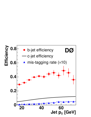
Figure 7: Measured $b$-tagging efficiency (circles) and mis-tagging rate (triangles), and estimated $c$-tagging efficiency (solid line) as a function of jet $p_{T}$.

To calculate the probability for a simulated jet to be tagged, a tag-rate function (TRF) derived from data is used similarly to the taggability parametrized in $p_{T}$ and $\eta$:

$$P^{\rm tagging}(p_{T},\eta)=\frac{{\rm\#\>SVT\>tagged\>jets\>in\>}(p_{T},\eta){\rm\>bin}}{{\rm\#\>taggable\>jets\>in\>}(p_{T},\eta){\rm\>bin}}.$$ (2)

Separate functions are determined for $b$-quark jets, $c$-quark jets, and light-quark jets, as in Fig. 7.

The TRFs are applied to the Monte Carlo samples in the following way. First, for each jet in the event (with $p_{T}>15$ GeV and $|\eta|<3.4$) a taggability-rate function is applied. Next, each jet’s lineage is determined. If the jet contains a $B$ meson within $R<0.5$ of the jet axis it is labeled a $b$-quark jet. If a $D$ meson is within $R<0.5$ of the jet axis, it is labeled a $c$-quark jet. If no $B$ or $D$ meson is found in the jet, the jet is labeled a light-quark jet. The probability determined from the appropriate TRF is then applied. The taggability and tagging probability are multiplied together to determine the probability of the simulated jet to be tagged.

In data we apply the secondary vertex algorithm directly and can identify which jet is tagged and which is not. The situation in simulated events is different; the TRFs return a probability (or weight) rather than a tagged/not-tagged answer per jet. Since many of the discriminant variables used later on in the analysis (see Sec. VII.1) need to know which jet was tagged, each possible combination of tagged and untagged jets is considered for every simulated event. Thus each event is used repeatedly in the analysis, considering each time a different jet as tagged. The probability of each combination is calculated using the tag rate functions, and combined with the overall event weight. The sum of the weights for all the possible combinations of each event is equal to the original probability for an event to have at least one tagged jet.

The use of all permissible tagged jet combinations in each simulated event is a very powerful tool. It ensures that the kinematic distributions in histograms of tagged events have the correct shape, and it allows tagged jet information to be used in variables for signal/background separation, since the final classifiers are trained with weighted events.

III Triggers and Data Set

The DØ trigger system is composed of three levels. The first level consists of hardware and firmware components, the second level uses information from the first level to construct simple physics objects, and the third level is software based and performs full event reconstruction.

The DØ calorimeter is used to trigger events based on the energy deposited in towers of size $\Delta\eta\times\Delta\phi=0.2\times 0.2$ that are segmented longitudinally into electromagnetic and hadronic sections. The level 1 electron trigger requires electrons to be above a certain threshold: $E_{T}\equiv E\sin\theta>T$ where $E$ is the energy deposited in the tower, $\theta$ is the angle between the beam and the trigger tower from the center of the detector, and $T$ is the programmed threshold. The level 2 electron trigger uses a seed-based clustering algorithm that sums the energy deposited in two neighboring towers and has the ability to make a decision based on the threshold of the cluster, the electromagnetic fraction, and isolation of the electron. The level 3 electron trigger uses a simple cone algorithm with $R<0.25$ and requirements on the $E_{T}$, the electromagnetic fraction, and the quality of the transverse shower shape.

The level 1 jet trigger is similar to the electron trigger tower algorithm, but includes the energy deposited in the hadronic portion of the calorimeter. The level 2 jet trigger uses a seed-based clustering algorithm summing the energy deposition in a $5\times 5$ tower array. The level 3 jet algorithm is similar to the level 3 electron algorithm, but does not include a requirement on the electromagnetic fraction or shower shape.

The level 1 muon trigger examines hits from the muon wire chambers, muon scintillation counters, and tracks from the level 1 track trigger for patterns consistent with those coming from a muon. The level 2 muon trigger reconstructs muon tracks from both wire and scintillator elements in the muon system. It can impose requirements on the number of muons, the $p_{T}$ and $\eta$ of the muons, and the overall quality of the muons. The level 3 muon trigger uses wire and scintillator hits to reconstruct tracks using segments inside and outside the toroid.

The output of the first level of the trigger is used to limit the rate for accepted events to $\approx$ 1.5 kHz. At the next trigger stage, with more refined information, the rate is reduced further to $\approx$ 800 Hz. The third level of the trigger, with access to all the event information, reduces the output rate to $\approx$ 50 Hz, which is written to tape.

The data were acquired in the period between August 2002 and March 2004. Tables 2 and 3 show the triggers used to collect the data for the electron plus jets ($e$+jets) and muon plus jets ($\mu$+jets) triggers and give the integrated luminosity for each trigger.

Table 2: Trigger conditions at levels 1, 2, and 3 for the electron plus jets trigger.

Level 1	Level 2	Level 3	Luminosity
Condition	Condition	Condition
1 EM tower, $E_{T}>10$ GeV	1 $e$, $E_{T}>10$ GeV, EM fraction $>0.85$	1 tight $e$, $E_{T}>15$ GeV	19.4 pb-1
2 jet towers, $E_{T}>5$ GeV	2 jets, $E_{T}>10$ GeV	2 jets, $E_{T}>15$ GeV
1 EM tower, $E_{T}>10$ GeV	1 $e$, $E_{T}>10$ GeV, EM fraction $>0.85$	1 loose $e$, $E_{T}>15$ GeV	91.2 pb-1
2 jet towers, $E_{T}>5$ GeV	2 jets, $E_{T}>10$ GeV	2 jets, $E_{T}>15$ GeV
1 EM tower, $E_{T}>11$ GeV		1 tight $e$, $E_{T}>15$ GeV	115.4 pb-1
		2 jets, $E_{T}>20$ GeV

Table 3: Trigger conditions at levels 1, 2, and 3 for the muon plus jets trigger.

Level 1	Level 2	Level 3	Luminosity
Condition	Condition	Condition
1 $\mu$, $\mid\eta\mid<2.0$	1 $\mu$, $\mid\eta\mid<2.0$	1 jet, $E_{T}>20$ GeV	113.7 pb-1
1 jet tower, $E_{T}>5$ GeV
1 $\mu$, $\mid\eta\mid<2.0$	1 $\mu$, $\mid\eta\mid<2.0$	1 jet, $E_{T}>25$ GeV	113.7 pb-1
1 jet tower, $E_{T}>3$ GeV	1 jet, $E_{T}>10$ GeV

IV Event Selection

Event selection begins after all corrections have been applied to the data. These corrections include the jet energy and the EM energy calibrations. The primary vertex, $z_{\rm vertex}$, for the event must be within the tracking fiducial region, $|z_{\rm vertex}|<60$ cm, which allows for a sufficient number of tracks, $N_{\rm tracks}\geq 3$, associated with it to be properly reconstructed.

As discussed in Sec. I.3, the single top quark signature is characterized by one isolated high-$p_{T}$ charged lepton, $\not\!\!E_{T}$, and two to four jets. We accept events with three or four jets in order to include contributions from extra gluons and quarks. The $b$ jet from the single top quark decay tends to be more energetic than the other jets associated with the event, so we require a higher $E_{T}$ for the leading jet. Table 4 lists the requirements of the initial selection.

Table 4: Initial event selection requirements.

Selection Cut	$e$+jets		$\mu$+jets
tight $e$, $E_{T}\geq$ 15 GeV	=1		=0
tight $\mu$, $E_{T}\geq$ 15 GeV	=0		=1
$\not\!\!E_{T}$		$\geq$ 15 GeV
$N_{\rm jets}$		$2\leq N_{\rm jets}\leq 4$
$E_{T}({\rm jet})$		$\geq 15$ GeV
$|\eta({\rm jet})|$		$\leq 3.2$
$E_{T}({\rm jet1})$		$\geq 25$ GeV
$|\eta({\rm jet1})|$		$\leq 2.4$

In addition, we make a set of cuts that remove misreconstructed events, also known as “triangle cuts.” If the transverse energy of an object is mismeasured, this tends to create false missing energy in a parallel or antiparallel direction. The triangle cuts remove these mismeasured events, which are difficult to model, but do not affect the signal appreciably because there is very small signal acceptance in these kinematic regions. In Fig. 8, we show the kinematic regions that are removed by the triangle cuts.

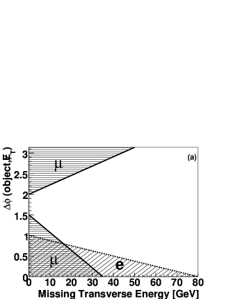
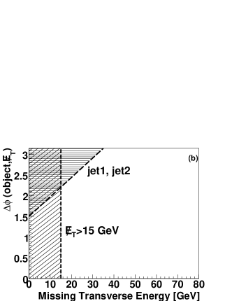
Figure 8: Kinematic regions excluded in the $e$+jets and $\mu$+jets analyses by the triangle cuts applied in the $(\Delta\phi({\rm object},\mbox{$\not\!\!E_{T}$}),\mbox{$\not\!\!E_{T}$})$ plane, where each object can be: the tight isolated electron or muon (a), and the leading and second leading jets (b). The shaded areas are excluded.

From the selected jets in the event, at least one $b$-tagged jet must be found. For the $t$-channel analysis, at least one jet must be untagged. This requirement comes from the fact that one of the main features of the $t$-channel signal is that a light-quark jet exists in the final state. The events are then divided into subsets consisting of the number of tagged jets found in the event: single-tagged or double-tagged. Since the $t$-channel requires at least one untagged jet, there are no two-jet events in the double-tagged sample in the double-tagged $t$-channel search.

V Signal and Background Modeling

In order to compare the observed event yield in data with our expectation, and to set limits on the single top quark production cross sections, we determine acceptances and event yields for the single top quark signals and the various SM background contributions. This estimation is based primarily on simulated samples for shapes of distributions, except for the multijet background where we use data samples. The yield normalization is based on theoretical cross sections, except for the $W$+jets and multijet backgrounds which are normalized to data.

V.1 Acceptance and Yield for Simulated Samples

The acceptance $\alpha$ for a particular simulated signal or background sample is calculated as:

$${\alpha}=\frac{1}{N^{\rm MC}}\sum_{i}w_{i}$$ (3)

where the sum is over simulated events that pass the selection cuts and is normalized to the total number of simulated events in the sample $N^{\rm MC}$. The event weight $w_{i}$ is given by:

$$w_{i}=\epsilon^{\rm lepton\;ID}_{i}\times\epsilon^{\rm jet\;ID}_{i}\times\epsilon^{\rm trigger}_{i}\times\epsilon^{b\;{\rm tagging}}_{i}$$ (4)

and includes correction factors $\epsilon$ to account for effects not modeled and for cuts not applied to the simulated samples. Trigger requirements are not made in the simulation (see Sec. III) and the correction factors $\epsilon^{\rm trigger}_{i}$ are about 90%. Furthermore, we do not require $b$ tagging in simulated events, and the correction factor $\epsilon^{b\;{\rm tagging}}_{i}$ averages about 55% for $s$-channel events and about 40% for $t$-channel events.

The yield estimate ${\cal Y}$ is given by the product of acceptance, integrated luminosity $\cal L$, theory cross section $\sigma^{\rm theory}$, and branching fraction B:

$${\cal Y}=\alpha\times{\cal L}\times\sigma^{\rm theory}\times{\it B}.$$ (5)

The branching fraction factor gives the fraction of events that result in the final state lepton of interest ($e$ or $\mu$). The yield includes a small contribution from $W\rightarrow\tau$ decays where the $\tau$ decays to $e$ or $\mu$.

V.2 Single Top Quark Signals

The Comphep matrix element generator comphepref has been used to model single top quark $s$-channel and $t$-channel signal events. We include not only the leading order Feynman diagrams in the event generation, but also the $O(\alpha_{s})$ diagrams with real gluon radiation in order to reproduce NLO distributions. For the $t$-channel sample, we include both the leading order diagram (Fig. 2 (a)) and the $W$-gluon fusion diagram (Fig. 2 (b)) explicitly, generating $W$-gluon fusion events for the region of phase space where the $\bar{b}$ quark from gluon splitting has $p_{T}(\mbox{$\bar{b}$})>17$ GeV and leading order events otherwise.

V.3 $t\bar{t}$ Background

Top quark pair production contributes as a background both in the lepton+jets and in the dilepton decay channels. This background is modeled using alpgen Mangano:2002ea , and the yields are normalized to the theory cross section (see Sec. I.3).

V.4 $WW$ and $WZ$ Backgrounds

The backgrounds from diboson production are modeled using alpgen, and the yields are normalized to the theory cross sections Campbell:1999ah .

V.5 Multijet and $W$+jets Backgrounds

The backgrounds from multijet (fake lepton) and $W$+jets production are normalized to the data sample before $b$ tagging top-cs-topo . We start from a data sample passing all selection cuts including the loose lepton requirements (see Sec. II.2). From that sample, we select a subset of events that also pass the tight lepton requirements. In addition, we determine the probabilities for real and fake leptons to pass the tight lepton requirement. These two probabilities together with the numbers of events in the two samples then allow us to calculate the number of real and fake lepton events in the $W$+jets and multijet background samples Abbott:1999tt .

The shapes of the distributions for the multijet background are modeled using a data sample that passes all selection cuts but fails the tight lepton identification requirements. The shapes of distributions for the $W$+jets background are modeled using alpgen $W$+2jets events.

V.5.1 Multijet Background

A part of the background comes from events in which jets are misidentified as isolated leptons. In the electron channel, this background is typically produced by jets that contain a $\pi^{0}$, which, together with a randomly associated track, is misreconstructed as an isolated electron since it decays to two photons. In the muon channel, this background is typically produced by heavy-flavor jets in which a muon from a semileptonic decay is misreconstructed as an isolated high-$p_{T}$ muon.

The multijet background is estimated purely from data. We use multijet data samples that pass all event selection requirements, but fail the requirement on tight muon isolation or tight electron quality (see Sec. II.2) to determine the kinematic shape of distributions. These samples are normalized to the multijet background estimate in the data sample after event selection, but before requiring a $b$ tag.

V.5.2 $W$+Jets Background

An example Feynman diagram for $W$+2 jet production is shown in Fig. 9. This background is modeled from a simulated $Wjj$ sample ($j=u,d,s,c,g$), which includes not just light-quark flavors but also $c$ quarks (considered massless in this model). We use a separate sample for $Wb\bar{b}$ and explicitly exclude events with $b$ quarks from the $Wjj$ sample. The parton level samples were generated with alpgen.

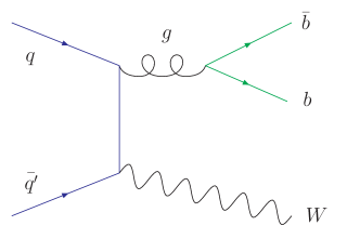
Figure 9: Representative Feynman diagram for $Wb\bar{b}$ production.

Since the $W$+jets background is normalized to data (after subtraction of the small $t\bar{t}$ and diboson content), it includes all sources of $W$+jets events with a similar flavor composition, in particular $Z$+jets events where one of the leptons from the $Z$ boson decay is not identified.

V.6 Detector Simulation

The parton-level samples for the single top quark signals, $t\bar{t}$, $W$+jets, $WW$, and $WZ$ backgrounds are processed with pythia pythiaref for hadronization and modeling of the underlying event, using the cteq5l cteqref parton distribution functions. tauola Jadach:1990mz is used for tau lepton decays and evtgen Lange:2001uf for $B$ hadron decays. The generated events are processed through a geant-based geantref simulation of the DØ detector.

VI Event Yields

The expected event yields for the various background contributions are calculated from both simulated samples and data. The expected event yield for the single top quark signal is calculated from simulated samples and normalized to the theoretical cross sections.

The total background event yield $\cal{Y}$ is given by the sum over all backgrounds:

$${\cal{Y}}=\sum_{i}{\cal{Y}}_{i}$$ (6)

where each individual yield ${\cal{Y}}_{i}$ is given by Eq. 5 for the various MC samples.

Table 5 shows the numbers of events for each of the signals, combinations of signals, backgrounds, and data, after event selection and $b$ tagging. The background sum reproduces the data within uncertainties for all samples after $b$ tagging.

Table 5: Event yields after selection in the electron and muon channels.

	Electron Channel				Muon Channel
	before tag	=1 tag	$\geq$2 tags	$\geq$2 tags	before tag	=1 tag	$\geq$2 tags	$\geq$2 tags
			$s$-channel	$t$-channel			$s$-channel	$t$-channel
Signals
$tb$	5	2.3	0.53	—	5	2.2	0.50	—
$tqb$	12	4.1	—	0.25	11	3.9	—	0.23
Backgrounds
$tb$	—	—	—	0.14	—	—	—	0.13
$tqb$	—	—	0.32	—	—	—	0.29	—
${\mbox{$t\bar{t}$}}{\mbox{$\rightarrow$}}\ell$+jets	59	25.0	6.12	5.74	58	24.2	5.78	5.48
${\mbox{$t\bar{t}$}}{\mbox{$\rightarrow$}}\ell\ell$	16	6.8	1.58	0.74	17	7.2	1.62	0.75
$Wb\bar{b}$	40	15.1	2.49	0.59	33	12.7	2.15	0.55
$Wjj$	3,211	68.2	1.53	0.66	2,898	62.9	1.29	0.68
$WW$	13	0.7	0.00	0.00	14	0.7	0.00	0.00
$WZ$	4	0.6	0.11	0.02	5	0.5	0.09	0.01
Multijet	478	13.7	0.31	0.14	256	17.2	0.20	0.20
Summed signals	17	6.4	0.53	0.25	16	6.0	0.50	0.23
Summed backgrounds	3,821	130.1	—	—	3,280	125.4	—	—
Summed backgrounds+$tqb$	3,833	134.2	12.47	—	3,291	129.3	11.43	—
Summed backgrounds+$tb$	3,826	132.4	—	8.03	3,285	127.6	—	7.80
Data	3,821	134	15	11	3,280	118	16	8

A summary of the yield estimates for the signal and backgrounds and the numbers of observed events in data after selection, including the systematic uncertainties as described in Sec. VIII, is shown in Table 6.

Table 6: Estimates for signal and background yields and the numbers of observed events in data after event selection for the electron and muon, single-tagged and double-tagged analysis sets combined. The $W$+jets yields include the diboson backgrounds. The total background for the $s$-channel ($t$-channel) search includes the $tqb$ ($tb$) yield. The quoted yield uncertainties include systematic uncertainties taking into account correlations between the different analysis channels and samples.

Source	$s$-channel search		$t$-channel search
$tb$	5.5$\,\pm\!\!\!\!$	1.2	4.8$\,\pm\!\!\!\!$	1.0
$tqb$	8.6$\,\pm\!\!\!\!$	1.9	8.5$\,\pm\!\!\!\!$	1.9
$W$+jets	169.1$\,\pm\!\!\!\!$	19.2	163.9$\,\pm\!\!\!\!$	17.8
$t\bar{t}$	78.3$\,\pm\!\!\!\!$	17.6	75.9$\,\pm\!\!\!\!$	17.0
Multijet	31.4$\,\pm\!\!\!\!$	3.3	31.3$\,\pm\!\!\!\!$	3.2
Total background	287.4$\,\pm\!\!\!\!$	31.4	275.8$\,\pm\!\!\!\!$	31.5
Observed events	283		271

After $b$ tagging, the $W$+jets background makes up around 60% of the total background model (48% $Wjj$, 12% $Wb\bar{b}$), the $t\bar{t}$ background is around 27% (21% lepton+jets, 6% dilepton), 10% is mainly multijet background, and $s$-channel single top quark production provides $3\%$ in the $t$-channel search and vice versa.

VII Event Analysis

Table 5 shows that even after event selection and $b$ tagging, the expected single top quark signal yield is small compared to the overwhelming backgrounds. Additional steps are necessary in order to separate the signal and background. In this section, we first present kinematic variables that allow us to separate the $s$-channel or $t$-channel single top quark signal from the backgrounds. We then describe a cut-based analysis and a neural networks analysis that use these variables.

VII.1 Discriminating Variables

In this section we introduce the variables that we found to be most effective in separating the single top quark signals from the backgrounds. The list of discriminating variables has been chosen based on an analysis of Feynman diagrams of signals and backgrounds boos-dudko and on a study of single top quark production at NLO sintop-nlo-sch ; sintop-nlo-tch .

The variables fall into three categories: individual object kinematics, global event kinematics, and variables based on angular correlations. The list of variables is shown in Table 7.

In order to get optimum separation between signal and background, the single top quark final state is reconstructed according to whether a variable is primarily used in the $s$-channel or the $t$-channel search. The $W$ boson from the top quark decay is reconstructed from the isolated lepton and the missing transverse energy. The $z$-component of the neutrino momentum is calculated using a $W$ boson mass constraint, choosing the solution with smaller $|p^{\nu}_{z}|$ from the two possible solutions. The candidate top quark is reconstructed from this $W$ boson and a jet. This jet is chosen to be either the leading $b$-tagged jet or the $best$ jet. In the $t$-channel analysis, there is typically only one high-$p_{T}$ $b$ quark jet in the final state, thus the leading $b$-tagged jet is chosen to reconstruct the top quark. By contrast, in the $s$-channel there are two high-$p_{T}$ $b$ quark jets in the final state, and a choice needs to be made between them. Furthermore, typically only one of the two is identified as a $b$-tagged jet. We use the best-jet algorithm d0runI to identify this jet without using $b$ tagging information. The best jet is defined as the jet in each event which gives, together with the reconstructed $W$ boson, an invariant mass closest to 175 GeV. Jets that have not been identified by the $b$ tagging algorithm are called “untagged” jets.

Table 7: List of discriminating variables. A check mark in the final four columns indicates in which signal-background pair of the neural net analysis the variable is used.

Signal-Background Pairs
		$tb$		$tqb$
Variable	Description	$W\mbox{$b\bar{b}$}$	$t\bar{t}$	$W\mbox{$b\bar{b}$}$	$t\bar{t}$
Individual object kinematics
$p_{T}({\rm jet1}_{\rm tagged})$	Transverse momentum of the leading tagged jet	$\surd$	$\surd$	$\surd$	—
$p_{T}({\rm jet1}_{\rm untagged})$	Transverse momentum of the leading untagged jet	—	—	$\surd$	$\surd$
$p_{T}({\rm jet2}_{\rm untagged})$	Transverse momentum of the second untagged jet	—	—	—	$\surd$
$p_{T}({\rm jet1}_{\rm non-best})$	Transverse momentum of the leading non-best jet	$\surd$	$\surd$	—	—
$p_{T}({\rm jet2}_{\rm non-best})$	Transverse momentum of the second non-best jet	$\surd$	$\surd$	—	—
Global event kinematics
$\sqrt{\hat{s}}$	Invariant mass of all final state objects	$\surd$	—	$\surd$	$\surd$
$p_{T}({\rm jet1},{\rm jet2})$	Transverse momentum of the two leading jets	$\surd$	—	$\surd$	—
$M_{T}({\rm jet1},{\rm jet2})$	Transverse mass of the two leading jets	$\surd$	—	—	—
$M({\rm alljets})$	Invariant mass of all jets	$\surd$	$\surd$	$\surd$	$\surd$
$H_{T}({\rm alljets})$	Sum of the transverse energies of all jets	—	—	$\surd$	—
$p_{T}({\rm alljets}-{\rm jet1}_{\rm tagged})$	Transverse momentum of all jets excluding the leading tagged jet	—	$\surd$	—	$\surd$
$M({\rm alljets}-{\rm jet1}_{\rm tagged})$	Invariant mass of all jets excluding the leading tagged jet	—	—	—	$\surd$
$H({\rm alljets}-{\rm jet1}_{\rm tagged})$	Sum of the energies of all jets excluding the leading tagged jet	—	$\surd$	—	$\surd$
$H_{T}({\rm alljets}-{\rm jet1}_{\rm tagged})$	Sum of the transverse energies of all jets excluding the leading tagged jet	—	—	—	$\surd$
$M(W,{\rm jet1}_{\rm tagged})$	Invariant mass of the reconstructed top quark using the leading tagged jet	$\surd$	$\surd$	$\surd$	$\surd$
$M({\rm alljets-jet_{best}})$	Invariant mass of all jets excluding the best jet	—	$\surd$	—	—
$H({\rm alljets}-{\rm jet}_{\rm best})$	Sum of the energies of all jets excluding the best jet	—	$\surd$	—	—
$H_{T}({\rm alljets}-{\rm jet}_{\rm best})$	Sum of the transverse energies of all jets excluding the best jet	—	$\surd$	—	—
$M(W,{\rm jet}_{\rm best})$	Invariant mass of the reconstructed top quark using the best jet	$\surd$	—	—	—
Angular variables
$\eta({\rm jet1}_{\rm untagged})\times Q_{\ell}$	Pseudorapidity of the leading untagged jet $\times$ lepton charge	—	—	$\surd$	$\surd$
$\Delta\cal{R}({\rm jet1},{\rm jet2})$	Angular separation between the leading two jets	$\surd$	—	$\surd$	—
$\cos({\rm\ell},{\rm jet1}_{\rm untagged})_{\rm top_{tagged}}$	Top quark spin correlation in the optimal basis for the $t$-channel Mahlon:1995zn , reconstructing the top quark with the leading tagged jet	—	—	$\surd$	—
$\cos({\rm\ell},Q_{\ell}$$\times$$z)_{\rm top_{best}}$	Top quark spin correlation in the optimal basis for the $s$-channel Mahlon:1995zn , reconstructing the top quark with the best jet	$\surd$	—	—	—
$\cos({\rm alljets},{\rm jet1}_{\rm tagged})_{\rm alljets}$	Cosine of the angle between the leading tagged jet and the alljets system in the alljets rest frame	—	—	$\surd$	$\surd$
$\cos({\rm alljets},{\rm jet}_{\rm non-best})_{\rm alljets}$	Cosine of the angle between the leading non-best jet and the alljets system in the alljets rest frame	—	$\surd$	—	—

Figures 10 to 14 show all discriminating variables used in this analysis, comparing the single top quark signal distributions to those of the background sum and the data. Good agreement between the data and the background model is seen in all cases.

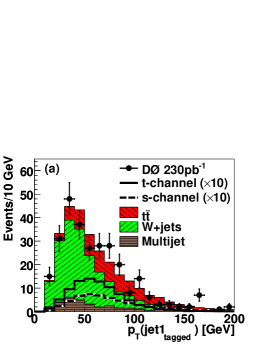
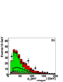
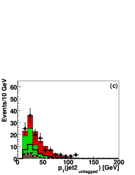
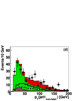
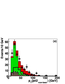
Figure 10: Comparison of signal, backgrounds, and data after selection and requiring at least one $b$-tagged jet for five individual object variables. Electron and muon channels are combined. The transverse momentum is shown for (a) the leading tagged jet; (b) the leading untagged jet; (c) the second untagged jet, for those events that contain at least two untagged jets; (d) the leading non-best jet; and (e) the second non-best jet. Signals are multiplied by ten.

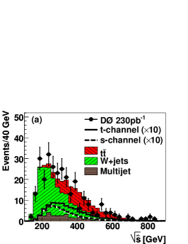
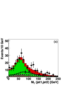
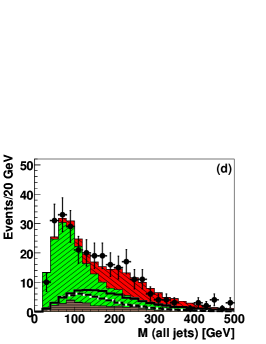
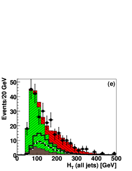
Figure 11: Comparison of signal, backgrounds, and data after selection and requiring at least one $b$-tagged jet for five discriminating event kinematic variables. Electron and muon channels are combined. Shown are (a) the invariant mass of all final state objects, (b) the total transverse momentum of the leading two jets, (c) the transverse mass of the leading two jets, (d) the invariant mass of all jets, and (e) the total transverse energy of all jets. Signals are multiplied by ten.

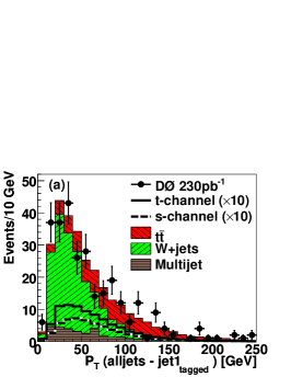
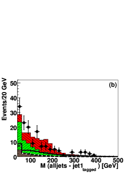
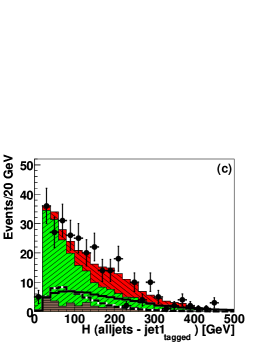
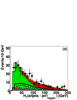
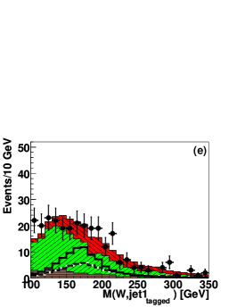
Figure 12: Comparison of signal, backgrounds, and data after selection and requiring at least one $b$-tagged jet for five discriminating event kinematic variables. Electron and muon channels are combined. Shown are (a) the transverse momentum of all jets except the leading tagged jet, (b) the invariant mass of all jets except the leading tagged jet, (c) the total energy of all jets except the leading tagged jet, (d) the total transverse energy of all jets except the leading tagged jet, and (e) the invariant mass of the top quark reconstructed from the reconstructed $W$ boson and the leading tagged jet. Signals are multiplied by ten.

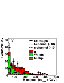
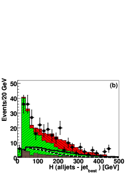
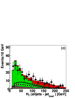
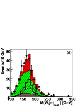
Figure 13: Comparison of signal, backgrounds, and data after selection and requiring at least one $b$-tagged jet for four discriminating event kinematic variables. Electron and muon channels are combined. Shown are (a) the invariant mass of all jets except the best jet, (b) the total energy of all jets except the best jet, (c) the total transverse energy of all jets except the best jet, and (d) the invariant mass of the top quark reconstructed from the reconstructed $W$ boson and the best jet. Signals are multiplied by ten.

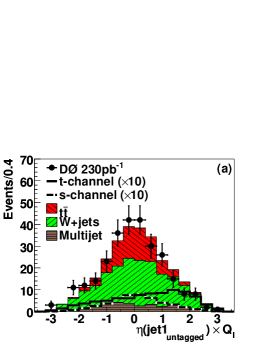
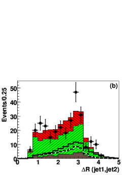
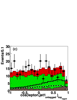
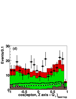
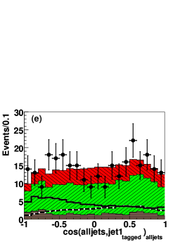
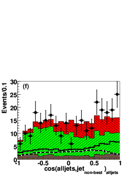
Figure 14: Comparison of signal, backgrounds, and data after selection and requiring at least one $b$-tagged jet for six angular correlation variables. Electron and muon channels are combined. Shown are (a) the pseudorapidity of the leading untagged jet multiplied by the lepton charge; (b) the angular separation between the leading two jets; (c) the top quark spin correlation in the optimal basis for the $t$-channel; (d) the top quark spin correlation in the optimal basis for the $s$-channel; (e) the cosine of the angle between the leading tagged jet and alljets, in the alljets frame; and (f) the cosine of the angle between the leading non-best jet and alljets, in the alljets frame. Signals are multiplied by ten.

VII.2 Cut-Based Analysis

This analysis takes the discriminating variables, chooses the best subsets, and finds the optimal points to cut on them in order to improve the expected cross section limits by increasing the signal to background ratio.

Optimization of the cut positions is performed by using the signal Monte Carlo events to seed the cut values scanned in the algorithm. The signal and background pass rates are determined for each cut point, an expected limit on the cross section is obtained from these, and the best result is used as the operating point of the analysis.

The strategy is to look at the $s$- and $t$-channel processes separately to take full advantage of the kinematical differences between the channels. For each channel, there are four orthogonal analyses: two leptons ($e$, $\mu$) $\times$ number of tagged $b$ jets ($=1$, $\geq 2$).

The most critical part of this analysis is to find the combination of variables and cuts that leads to the lowest expected cross section limit. We first look at single-variable cuts to determine which variables are most effective in each channel. Once an ordered list of variables is found (ordered by their power to lower the expected limit), sets of variables are formed starting with the best variable and consecutively including one-by-one the rest of the variables. For each set, the optimal cut position of each variable is recalculated. Finally, the variable set that gives the lowest expected limit is chosen. Table 8 shows the optimal variable sets and cuts found for each channel. Table 9 shows the numbers of events and expected background and signal yields after these cuts have been applied.

Table 8: The best set of variables and cuts for each analysis channel.

	$s$-channel		$t$-channel
Channel	Variables	Cuts	Variables	Cuts
Electron
=1 tag	$p_{T}$(jet1tagged)	$>27$ GeV	$H_{T}({\rm alljets})$	$>71$ GeV
	$M({\rm alljets-jet1_{tagged}})$	$<70$ GeV	$M({\rm alljets})$	$>57$ GeV
	$\sqrt{\hat{s}}$	$>196$ GeV	$\sqrt{\hat{s}}$	$>203$ GeV
			$\left|175-M(W,{\rm jet1_{tagged}})\right|$	$<57$ GeV
			$p_{T}$(jet1tagged)	$>21$ GeV
$\geq$2 tags	$p_{T}$(jet1tagged)	$>42$ GeV	$p_{T}$(jet1tagged)	$>34$ GeV
	$M({\rm alljets-jet1_{tagged}})$	$<98$ GeV	$M({\rm alljets-jet1_{tagged}})$	$<75$ GeV
	$H({\rm alljets-jet_{best}})$	$<304$ GeV	$H({\rm alljets-jet1_{tagged}})$	$<504$ GeV
	$H({\rm alljets-jet1_{tagged}})$	$<304$ GeV	$H({\rm alljets-jet_{best}})$	$<504$ GeV
Muon
=1 tag	$p_{T}$(jet1tagged)	$>33$ GeV	$\left|175-M(W,{\rm jet1_{tagged}})\right|$	$<60$ GeV
	$M({\rm alljets-jet1_{tagged}})$	$<74$ GeV	$\sqrt{\hat{s}}$	$>210$ GeV
	$H({\rm alljets-jet_{best}})$	$<504$ GeV	$M({\rm alljets})$	$>70$ GeV
	$H({\rm alljets-jet1_{tagged}})$	$<504$ GeV	$H_{T}({\rm alljets})$	$>58$ GeV
$\geq$2 tags	$p_{T}$(jet1tagged)	$>33$ GeV	$\left|175-M(W,{\rm jet1_{tagged}})\right|$	$<213$ GeV
	$M({\rm alljets-jet1_{tagged}})$	$<74$ GeV
	$H({\rm alljets-jet_{best}})$	$<504$ GeV
	$H({\rm alljets-jet1_{tagged}})$	$<504$ GeV

Table 9: Event yields after the cut-based analysis selection.

	Electron Channel				Muon Channel
	=1 Tag		$\geq$2 Tags		=1 Tag		$\geq$2 Tags
	$s$-channel	$t$-channel	$s$-channel	$t$-channel	$s$-channel	$t$-channel	$s$-channel	$t$-channel
Signals
$tb$	1.7	—	0.45	0.12	1.9	—	0.43	—
$tqb$	—	3.4	—	0.23	—	3.1	—	0.23
Backgrounds
$tb$	—	1.6	—	0.12	—	1.4	—	0.12
$tqb$	2.5	—	0.14	—	2.8	—	0.01	—
${\mbox{$t\bar{t}$}}{\mbox{$\rightarrow$}}\ell$+jets	3.8	18.5	1.14	4.61	9.7	17.8	0.61	5.20
${\mbox{$t\bar{t}$}}{\mbox{$\rightarrow$}}\ell\ell$	4.3	4.1	1.15	0.62	5.8	4.3	1.12	0.73
$Wb\bar{b}$	8.4	6.3	1.72	0.54	10.2	5.2	1.85	0.52
$Wjj$	33.4	28.9	0.74	0.60	43.6	28.8	0.95	0.64
$WW$	0.4	0.3	0.01	0.00	0.6	0.3	0.00	0.00
$WZ$	0.4	0.3	0.09	0.01	0.4	0.2	0.09	0.01
Multijet	6.8	6.9	0.20	0.14	10.1	9.9	0.11	0.01
Summed signals	4.3	4.9	0.59	0.35	4.7	4.5	0.53	0.35
Summed backgrounds	57.5	65.3	5.04	6.54	80.3	66.7	4.71	7.20
Summed backgrounds+$tqb$	60.0	68.6	5.18	6.76	83.1	69.8	4.81	7.43
Summed backgrounds+$tb$	59.2	66.8	5.49	6.65	82.2	68.1	5.14	7.32
Data	60	73	4	9	78	58	10	8

A summary of the yield estimates for the signal and backgrounds and the numbers of observed events in data after the cut-based selection, including the systematic uncertainties as described in Sec. VIII, is shown in Table 10.

Table 10: Estimates of backgrounds and signal yields and the number of observed events in data after the cut-based selection for the electron and muon, =1 tag and $\geq$2 tags analyses combined.

Source	$s$-channel search		$t$-channel search
$tb$	4.5$\,\pm\!\!\!\!$	1.0	3.2$\,\pm\!\!\!\!$	0.8
$tqb$	5.5$\,\pm\!\!\!\!$	1.2	7.0$\,\pm\!\!\!\!$	1.6
$W$+jets	27.6$\,\pm\!\!\!\!$	7.6	55.9$\,\pm\!\!\!\!$	12.3
$t\bar{t}$	102.9$\,\pm\!\!\!\!$	13.7	72.6$\,\pm\!\!\!\!$	9.7
Multijet	17.2$\,\pm\!\!\!\!$	2.0	17.0$\,\pm\!\!\!\!$	2.0
Total background	153.1$\,\pm\!\!\!\!$	24.5	148.7$\,\pm\!\!\!\!$	24.8
Observed events	152		148

Ths $s$- and $t$-channel combined signal to background ratio improves from around 1/20 after the basic selection (Table 6) to around 1/14 after these cuts have been applied. It is clear that more sophisticated separation techniques are needed to isolate the signal better from the large backgrounds.

VII.3 Neural Network Analysis

A neural network is a multivariate statistical technique for separating signals from backgrounds. We use the mlpfit mlpfit package to construct and implement the networks. In order for a neural network to approach the maximal signal-background separation, some optimization is required. This occurs in three steps: 1) judicious choice of signal and background pairs, 2) selection of input variables, and 3) optimization of training parameters.

VII.3.1 Choice of Signal-Background Pairs

We have chosen to create networks trained on single top quark signals against the two dominant backgrounds: $W$+jets and $t\bar{t}$. For $W$+jets, we train using a $Wb\bar{b}$ Monte Carlo sample as this process best represents all $W$+jets processes. For $t\bar{t}$, we train on ${\mbox{$t\bar{t}$}}{\mbox{$\rightarrow$}}\ell$+jets which is the dominant background as opposed to the dilepton background which is small.

VII.3.2 Choice of Input Variables

We start from a set of discriminating variables that each show some signal-background separation as discussed in Sec. VII.1. Based on this, we optimize the input variables for each network by training with different combinations of variables and choosing the combination that produces the minimum testing error, which corresponds to the best signal-background separation.

We use the same variables for the electron and muon channel. However, owing to different resolutions and pseudorapidity ranges, we train the networks separately for the two.

VII.3.3 Neural Network Training

Each network is composed of three layers of nodes: input, hidden, and output. Testing and training event sets are created from simulated signal and background samples. We divide the input samples such that 60% of the events are used for training and the remaining 40% for testing. Training is effected with weighted events and the logarithm of all nonangular variables. We use a technique called early stopping early_stopping to determine the maximum number of epochs for training which prevents over-training.

Each network is further tuned by varying the number of hidden nodes between 10 and 30 and then selecting the number of hidden nodes that returns the smallest testing error.

VII.3.4 Neural Network Results

The above procedure produces eight unique networks: two signals ($s$-channel, $t$-channel) $\times$ two backgrounds ($Wb\bar{b}$, ${\mbox{$t\bar{t}$}}{\mbox{$\rightarrow$}}\ell$+jets) $\times$ two lepton flavors ($e$, $\mu$).

Figures 15 and 16 show the output variable distributions from the networks in the $s$-channel and $t$-channel searches for electrons and muons. From the figures, it can be seen that these networks are highly efficient at separating the single top quark signal from the ${\mbox{$t\bar{t}$}}{\mbox{$\rightarrow$}}\ell$+jets background. Studies have shown that these networks are not as effective for the $t\bar{t}$ dilepton background, which is fortunately small. The $s$-channel and $t$-channel networks are less efficient at separating the single top quark signal from the $Wb\bar{b}$ background as compared to ${\mbox{$t\bar{t}$}}{\mbox{$\rightarrow$}}\ell$+jets. In addition, we find these networks are equally effective in separating the $Wjj$ and the misidentified lepton background as compared to the $Wb\bar{b}$ background. It should be noted that the output variable from mlpfit networks is not restricted to lie between zero and one.

Figures 17 and 18 show comparisons of the summed backgrounds to data for the $s$-channel and $t$-channel searches, for electrons, muons, single-tagged, and double-tagged samples combined. These distributions show that the background model reproduces the data very well. From the figures, it can be seen that the ${\mbox{$t\bar{t}$}}{\mbox{$\rightarrow$}}\ell$+jets filters do indeed separate the $t\bar{t}$ background which clusters near zero, but does not affect the $W$+jets and multijet backgrounds, which cluster near one. Similarly, the $Wb\bar{b}$ filters discriminate the $W$+jets and multijet backgrounds, which cluster to the left of 0.5, but do not affect the $t\bar{t}$ background, which clusters to the right of 0.5. They also show that separation of the single top quark signal from background is not yet powerful enough since the background dominates even in the regions where the signal peaks.

Figure 19 shows the output of the $tb$-$t\bar{t}$ network versus the $tb$-$Wb\bar{b}$ network, and similarly for the $tqb$ networks, again for electrons, muons, single-tagged, and double-tagged events combined.

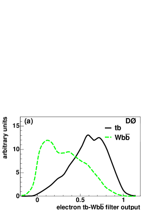
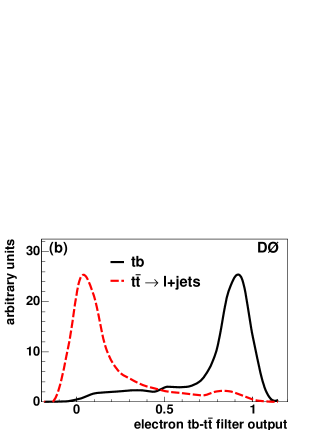
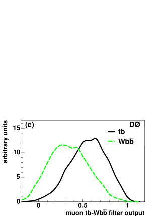
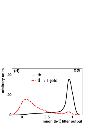
Figure 15: Neural network outputs in the $s$-channel. This figure shows the signal-background separation for (a) the filter for $Wb\bar{b}$ in the electron channel, (b) the filter for ${\mbox{$t\bar{t}$}}{\mbox{$\rightarrow$}}\ell$+jets in the electron channel, (c) the filter for $Wb\bar{b}$ in the muon channel, and (d) the filter for ${\mbox{$t\bar{t}$}}{\mbox{$\rightarrow$}}\ell$+jets in the muon channel where the background is the dashed-lined and the top quark signal is the solid line. All the curves are normalized to have equal area, so that the separation between signal and background can be best seen.

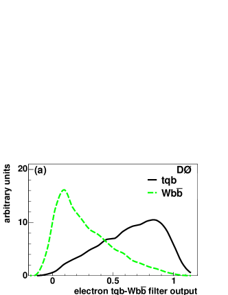
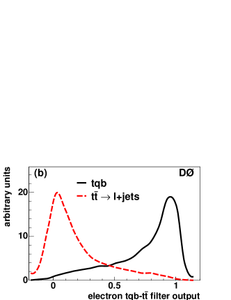
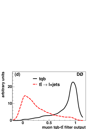
Figure 16: Neural network outputs in the $t$-channel. This figure shows the signal-background separation for (a) the filter for $Wb\bar{b}$ in the electron channel, (b) the filter for ${\mbox{$t\bar{t}$}}{\mbox{$\rightarrow$}}\ell$+jets in the electron channel, (c) the filter for $Wb\bar{b}$ in the muon channel, and (d) the filter for ${\mbox{$t\bar{t}$}}{\mbox{$\rightarrow$}}\ell$+jets in the muon channel where the background is the dashed-lined and the top quark signal is the solid line. All the curves are normalized to have equal area, so that the separation between signal and background can be best seen.

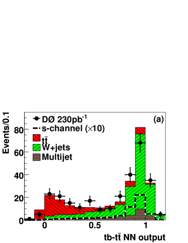
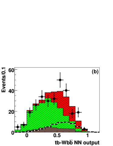
Figure 17: Comparison of signal, background, and data for the neural network outputs in the $s$-channel, for the electron and muon channels combined, requiring at least one $b$-tag. This figure shows (a) the $t\bar{t}$ filter and (b) the $Wb\bar{b}$ filter. Signals are multiplied by ten.

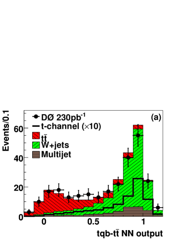
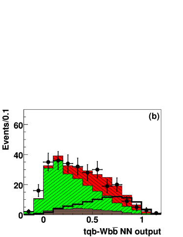
Figure 18: Comparison of signal, background, and data for the neural network outputs in the $t$-channel, for the electron and muon channels combined, requiring at least one $b$-tag. This figure shows (a) the $t\bar{t}$ filter and (b) the $Wb\bar{b}$ filter. Signals are multiplied by ten.

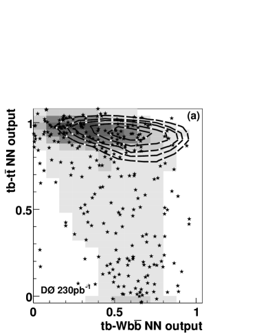
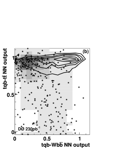
Figure 19: Neural network outputs for both the $t\bar{t}$ versus $Wb\bar{b}$ filters in the (a) $s$-channel (b) and $t$-channel analyses. The background sum is shown as the shaded area, the signal as contour lines, and the data as stars.

VIII Systematic Uncertainties

We consider several sources of systematic uncertainties in this analysis, and study them separately for each signal and background source. Some of the uncertainties affect acceptance for simulated signals and backgrounds, others only affect background yield estimates. This section lists the uncertainties for each signal and background and their correlations.

We consider the following sources of systematic uncertainty:

• The $b$-tag modeling uncertainty includes components for the estimation of the $b$ tagging efficiency in data for the various quark flavors, see Sec. II.3.

• The jet energy calibration uncertainty reflects how well jet energies measured in the simulation reflect jet energies measured in data, and includes jet energy scale uncertainty as well as modeling of jet energy resolution in the simulation, see Sec. II.2.

• The trigger modeling uncertainty includes components for the estimation of the efficiency of the various trigger requirements in data, see Sec. III.

• The jet fragmentation uncertainty covers the uncertainty in modeling of initial- and final-state radiation as well as the difference in the fragmentation model between pythia and herwig d0runI .

• The uncertainty on the correction factor for simulated samples to account for the jet identification efficiency as described in Sec. II.2.

• The uncertainty on the correction factor for lepton identification efficiency in simulated samples as described in Sec. II.2.

• The cross section and branching fraction uncertainties from the yield normalization of simulated backgrounds.

• The uncertainty on the normalization of the multijet and $W$+jets background yields to the data.

• The uncertainty on the integrated luminosity measurement.

The uncertainty on the multijet background normalization includes two components: the estimate of the rate to misidentify a jet as an isolated lepton in the data, and the $b$-tagging probability in the multijet data sample.

The uncertainty for the $Wjj$ and $Wb\bar{b}$ backgrounds includes several components: the normalization of the $W$+jets background to data before $b$ tagging, the $b$-tagging probability estimate, and the fraction of $Wb\bar{b}$ events in the $W$+jets sample. Owing to the normalization to data, the $Wb\bar{b}$ and $Wjj$ tagged yield estimates are not affected by any of the systematic uncertainties that affect the other simulated samples. The exception to this is $b$ tagging, which is applied after normalization. There is still an effect on the shape of the $Wjj$ and $Wb\bar{b}$ distributions from uncertainty components that vary bin-by-bin.

Table 11 shows the systematic uncertainty values for each signal and background component. The range is given for the different analysis channels, electron and muon as well as single tags and double tags.

Table 11: Range of relative systematic uncertainty values in percent for the various signal and background samples in the different analysis channels.

	$tb$	$tqb$	$t\bar{t}$	$W$+jets	multijet
Signal and background acceptance
$b$-tag modeling	5 – 20	8 – 20	6 – 20	7 – 20	—
Jet energy calibration	6 – 20	6 – 15	3 – 11	—	—
Trigger modeling	2 – 6	2 – 6	—	—	—
Jet fragmentation	5	5	7	—	—
Jet identification	1 – 13	5 – 11	1 – 4	—	—
Lepton identification	4	4	4	—	—
Background normalization
Theory cross sections	16	15	—	—	—
Normalization to data	—	—	—	5 – 16	5 – 16
Luminosity	6.5	6.5	6.5	—	—

Note that the $W$+jets background includes small contributions from $WW$ and $WZ$, whose uncertainties are also included in the limit setting calculation. Furthermore, the normalization for $Wb\bar{b}$ and $Wjj$ accounts for the other simulated backgrounds and thus their uncertainties in principle also affect $Wb\bar{b}$ and $Wjj$. However, the other simulated backgrounds only contribute about 3% to the pretagged yield, which means their uncertainties are negligible compared to the overall normalization uncertainties.

IX Cross Section Limits

We use a Bayesian approach IainTM2000 to calculate limits on the cross section for single top quark production in the $s$-channel and $t$-channel modes. The limits are derived from a likelihood function that is proportional to the probability to obtain the number of observed events. In the cut-based analysis, we count the total number of observed events, and in the neural network analysis, we use the two-dimensional distributions of the $t\bar{t}$ versus $Wb\bar{b}$ network outputs.

IX.1 Bayesian Approach

We assume that the probability to observe a count $D$, if the mean count is $d$, is given by the Poisson distribution:

$$p(D|d)=\frac{e^{-d}\,d^{D}}{\Gamma(D+1)}\,,$$ (7)

where $\Gamma$ is the gamma function. The mean count $d$ is a sum of the predicted contributions from the signal and background sources:

$$d=\alpha\,\mathcal{L}\,\sigma+\sum_{i=1}^{N}b_{i}\equiv a\sigma+\sum_{i=1}^{N}b_{i}\,,$$ (8)

where $\alpha$ is the signal acceptance, $\mathcal{L}$ the integrated luminosity, $\sigma$ the signal cross section (the quantity of interest), $b_{i}$ the mean count for background source $i$, and $a\equiv\alpha\,\mathcal{L}$ is the effective luminosity for the signal. For the $s$-channel ($t$-channel) search, the background $b_{i}$ includes the $t$-channel ($s$-channel) process. The likelihood function $L(D|d)$ is proportional to $p(D|d)$.

For two or more independent channels, we simply replace the single channel likelihood by a product of likelihoods:

$$L({\bf D}|{\bf d})\equiv L({\bf D}|\sigma,{\bf a},{\bf b})=\prod_{i=1}^{M}\,L(D_{i}|d_{i})\,,$$ (9)

where ${\bf D}$ and ${\bf d}$, respectively, represent vectors of the observed counts and the mean counts for the sources of signal and background, in the $M$ different channels. In addition, given $K$ bins of any distribution, we calculate the likelihood for each channel as the product of the individual likelihoods in each bin:

$$L(D_{i}|d_{i})=\prod_{j=1}^{K}\,L(D_{i,j}|d_{i,j})\,,$$ (10)

which is true if the probability to observe a count in a given bin is independent of the count in other bins.

We use Bayes’ theorem to compute the posterior probability density of the parameters, $p(\sigma,{\bf a},{\bf b}|{\bf D})$, which is then integrated with respect to the parameters ${\bf a}$ and ${\bf b}$ to obtain the posterior density for the signal cross section, given the observed distribution of counts ${\bf D}$:

$$p(\sigma|{\bf D})=\frac{1}{\mathcal{N}}\int\int L({\bf D}|\sigma,{\bf a},{\bf b})\pi(\sigma,{\bf a},{\bf b})\,d{\bf a}\,d{\bf b}\,.$$ (11)

Here $\mathcal{N}$ is an overall normalization obtained from the requirement $\int{p(\sigma|{\bf\rm D})}d\sigma=1$, and $\pi(\sigma,{\bf a},{\bf b})$ is the prior probability that encodes what we know about the parameters $\sigma$, ${\bf a}$ and ${\bf b}$. We assume that any prior knowledge of ${\bf a}$ and ${\bf b}$ is independent of the cross section $\sigma$, in which case we may write the prior density as

$$\pi(\sigma,{\bf a},{\bf b}) = \pi({\bf a},{\bf b}|\sigma)\,\pi(\sigma)\,$$ (12)

$$= \pi({\bf a},{\bf b})\,\pi(\sigma)\,.$$

We use a flat prior for $\sigma$: $\pi(\sigma)=1/\sigma_{\rm max}$, where $\sigma_{\rm max}$ is any sufficiently high upper bound on the cross section. The posterior probability density for the signal cross section is therefore

$$p(\sigma|{\bf D})=\frac{1}{\mathcal{N}}\int\int L({\bf D}|\sigma,{\bf a},{\bf b})\pi({\bf a},{\bf b})\,d{\bf a}\,d{\bf b}\,.$$ (13)

The Bayesian upper limit $\sigma_{\rm UL}$ at confidence level $\beta$ is the solution of

$$\int_{0}^{\sigma_{\rm UL}}p(\sigma|{\bf D})\,d\sigma\,=\beta\,.$$ (14)

The integral in Eq. 13 is done numerically using Monte Carlo importance sampling: we generate a large number $K$ of randomly sampled points $({\bf a}_{k},{\bf b}_{k})$ that represents the prior density $\pi({\bf a},{\bf b})$, and estimate the posterior using

$$\int\int L({\bf D}|\sigma,{\bf a},{\bf b})\pi({\bf a},{\bf b})\,d{\bf a}\,d{\bf b}=\frac{1}{K}\sum_{k=1}^{K}\,L({\bf D}|\sigma,{\bf a}_{k},{\bf b}_{k})\,.$$ (15)

IX.2 Definition of the Prior Probability

The prior $\pi({\bf a},{\bf b})$ encodes our knowledge of the effective signal luminosities and the background yields: we have estimates of the parameters and the associated uncertainties from the different systematic effects discussed in Sec. VIII. In the case of the cut-based analysis, since we consider the total yield for any source of signal or background, the different uncertainties affect the overall normalization only. In the neural network analysis, since we consider distributions, we separate the uncertainties into two classes: those that alter only the overall normalization, such as the luminosity measurement and theory cross sections; and those that also alter the shapes of distributions, such as the trigger modeling, jet energy calibration, jet energy resolution, jet identification, and $b$-tag modeling.

The normalization effects are modeled by sampling the effective signal luminosities a and the background yields b from a multivariate Gaussian, with a vector of means given by the estimates of the yields, and covariance matrix computed from the associated uncertainties. The covariance matrix takes into account the correlations of the systematic uncertainties across the different sources of signal and background. Each entry in the covariance matrix is calculated as follows:

$$c_{ij}=y_{i}y_{j}\sum_{k}f_{ik}f_{jk}\,,$$ (16)

where $y_{i}$ ($y_{j}$) is the yield for the $i^{\rm th}$ ($j^{\rm th}$) source of background or signal from Table 5, and $f_{ik}$ is the corresponding fractional uncertainty from the $k^{\rm th}$ component of systematic uncertainty, for the $i^{\rm th}$ source.

The shape effects are modeled by shifting, one by one, the trigger modeling, jet energy calibration, $b$-tag modeling, and so on, by plus or minus one standard deviation with respect to their nominal values. For each systematic effect, we have three distributions: the nominal, and those from the plus and minus shifts. The systematic uncertainty in each bin is then sampled from a Gaussian distribution with mean defined by the nominal yield in that bin, and width defined by the plus and minus shifts. The sampled shifts are added linearly to the yields generated from the sampling of the normalization-only systematic uncertainties. We assume that any shape-changing systematic is 100$\%$ correlated across all bins and sources.

X Results

For both the $s$-channel and $t$-channel searches, we compute an observed limit as well as an expected limit. We define the latter as the limit obtained if the observed counts were equal to the background prediction. The different tag multiplicities ($=1$ tag and $\geq 2$ tags) and lepton flavor (electron and muon) are combined as shown in Eq. 9.

The expected and observed upper limits at the 95% confidence level, after the initial event selection, and from the cut-based and neural network analyses, are shown in Table 12 for the electron and muon channels combined, and with all systematic effects included. We see that the limits improve upon applying cuts on the discriminating variables, but that tighter limits are obtained when the variables are combined using our neural networks method. The observed posterior probability densities as a function of the $s$-channel and $t$-channel cross sections are shown in Fig. 20 for the cut-based analysis and in Fig. 21 for the neural network analysis.

Table 12: Expected and observed upper limits (in picobarns) at the 95% confidence level, on the production cross sections of single top quarks in the $s$-channel ($tb$) and $t$-channel ($tqb$) searches, for the electron and muon channels combined, with all systematic effects included.

	Expected Limits		Observed Limits
	$tb$	$tqb$	$tb$	$tqb$
Initial selection	14.5	16.5	13.0	13.6
Cut-based	9.8	12.4	10.6	11.3
Neural networks	4.5	5.8	6.4	5.0

Figure 20: The observed posterior probability density as a function of the single top quark cross section for the cut-based analysis, for the electron and muon channels combined in the $s$-channel and the $t$-channel searches.

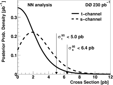
Figure 21: The observed posterior probability density as a function of the single top quark cross section for the neural network analysis, for the electron and muon channels combined in the $s$-channel and the $t$-channel searches.

The method described so far yields limits on the $s$-channel or $t$-channel cross sections separately. This requires some assumptions about whichever of the two signal processes is not being considered. In this particular analysis, we have assumed that in the $s$-channel ($t$-channel) search, the $t$-channel ($s$-channel) contributes as a SM background. This assumption is, however, not necessary. Instead, we can set limits on both the $s$-channel and $t$-channel cross sections simultaneously. We accomplish this by generalizing the likelihood so that it depends explicitly on the two cross sections $\sigma_{s}$ and $\sigma_{t}$. Equation 8 for the mean count $d$ then becomes:

$$d=\alpha_{s}\,\mathcal{L}\,\sigma_{s}+\alpha_{t}\,\mathcal{L}\,\sigma_{t}+\sum_{i}b_{i}\,.$$ (17)

The backgrounds $b_{i}$ now include only the non-single top quark sources.

In order to exploit the sensitivity to both the $s$-channel and $t$-channel signals, we combine the output of the neural networks in both searches. We calculate a signal probability $P$ in each bin of the histograms in Fig. 19:

$$P_{s(t)}=\frac{n_{s(t)}}{n_{s}+n_{t}+\sum_{i}b_{i}}\,,$$ (18)

for the $s$-channel ($t$-channel) search, where $n_{s}$ and $n_{t}$ are the yields for the $tb$ and $tqb$ samples, respectively, and the sum in the denominator is over all the non-single top quark backgrounds in that bin. We then evaluate $P_{s}$ and $P_{t}$ simultaneously for each event and fill histograms of $P_{s}$ versus $P_{t}$. As before, we consider a Poisson probability for the likelihood in each bin. We assume a flat prior in the plane of $\sigma_{s}$ versus $\sigma_{t}$, which is equivalent to flat priors for either cross section. Equations 13 and 15 can then be used to define the posterior probability density for different values of the $s$- and $t$-channel cross sections. The limit at a fixed confidence level is then given by a contour of constant probability enclosing a fraction of volume corresponding to this confidence level using an equation analogous to Eq. 14, but in two dimensions.

Figure 22 shows contours of observed posterior density in the $\sigma_{s}$ versus $\sigma_{t}$ plane for the neural network analysis. To illustrate the sensitivity of this analysis to different contributions, the expected SM cross section as well as several representative non-SM contributions are also shown Tait:2000sh .

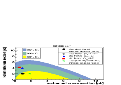
Figure 22: Exclusion contours at the 68%, 90%, and 95% confidence levels on the observed posterior density distribution as a function of both the $s$-channel and $t$-channel cross sections in the neural networks analysis. Several representative non-standard model contributions from Ref. Tait:2000sh are also shown.

XI Summary

We have analyzed electron+jet and muon+jet events containing exactly one or more than one $b$ jet, identified with a secondary-vertex algorithm, and find no evidence for the electroweak production of single top quarks in 230 pb^-1 of data collected by the DØ detector at $\sqrt{s}=1.96$ TeV. The upper limits at the 95% confidence level on the cross section for $s$-channel and $t$-channel processes are 10.6 pb and 11.3 pb, respectively, using event counts in a cut-based analysis, and 6.4 pb and 5.0 pb, respectively, using binned likelihoods in a neural network analysis. The neural network-base limits presented here and in Ref. RunII:d0_result are significantly more stringent than those previously published d0runI ; Acosta:2001un ; RunII:cdf_result . They are also close to the sensitivity required to probe models of physics beyond the standard model.

XII Acknowledgements

We thank the staffs at Fermilab and collaborating institutions, and acknowledge support from the DOE and NSF (USA); CEA and CNRS/IN2P3 (France); FASI, Rosatom and RFBR (Russia); CAPES, CNPq, FAPERJ, FAPESP and FUNDUNESP (Brazil); DAE and DST (India); Colciencias (Colombia); CONACyT (Mexico); KRF and KOSEF (Korea); CONICET and UBACyT (Argentina); FOM (The Netherlands); PPARC (United Kingdom); MSMT (Czech Republic); CRC Program, CFI, NSERC and WestGrid Project (Canada); BMBF and DFG (Germany); SFI (Ireland); The Swedish Research Council (Sweden); Research Corporation; Alexander von Humboldt Foundation; and the Marie Curie Program.

References

- (1)
- (2) On leave from IEP SAS Kosice, Slovakia.
- (3) Visitor from Helsinki Institute of Physics, Helsinki, Finland.
- (4) F. Abe et al. [CDF Collaboration], Phys. Rev. Lett. 74, 2626 (1995); S. Abachi et al. [DØ Collaboration], Phys. Rev. Lett. 74, 2632 (1995).
- (5) K. Hagiwara et al. [Particle Data Group Collaboration], Phys. Rev. D 66, 010001 (2002).
- (6) A.P. Heinson, A.S. Belyaev and E.E. Boos, Phys. Rev. D 56, 3114 (1997).
- (7) C. R. Chen, F. Larios and C. P. Yuan, Phys. Lett. B 631, 126 (2005).
- (8) T. Tait and C.-P. Yuan, Phys. Rev. D 63, 014018 (2001).
- (9) M.C. Smith and S. Willenbrock, Phys. Rev. D 54, 6696 (1996).
- (10) T. Stelzer, Z. Sullivan and S. Willenbrock, Phys. Rev. D 56, 5919 (1997).
- (11) B.W. Harris, E. Laenen, L. Phaf, Z. Sullivan and S. Weinzierl, Phys. Rev. D 66, 054024 (2002).
- (12) Z. Sullivan, Phys. Rev. D 70, 114012 (2004).
- (13) J. Campbell, R. K. Ellis, and F. Tramontano, Phys. Rev. D 70, 094012 (2004).
- (14) Q.-H. Cao, R. Schwienhorst, and C.-P. Yuan, Phys. Rev. D 71, 054023 (2005).
- (15) Q.-H. Cao, R. Schwienhorst, J. Benitez, R. Brock, and C.-P. Yuan, Phys. Rev. D 72, 094027 (2005).
- (16) R. Bonciani et al., Nucl. Phys. B 529, 424 (1998); M. Cacciari et al., JHEP 0404, 068 (2004); N. Kidonakis and R. Vogt, Phys. Rev. D 68, 114014 (2003).
- (17) Pseudorapidity is defined as , where is the polar angle with the origin at the primary vertex.
- (18) G. Mahlon and S. Parke, Phys. Rev. D 53, 4886 (1996); S. Parke and Y. Shadmi, Phys. Lett. B 387, 199 (1996); G. Mahlon and S. J. Parke, Phys. Rev. D 55, 7249 (1997).
- (19) E. E. Boos and A. V. Sherstnev, Phys. Lett. B534, 97 (2002).
- (20) M. L. Mangano et al., JHEP 0307, 001 (2003).
- (21) S. Mrenna and P. Richardson, arXiv:hep-ph/0312274 (2003).
- (22) B. Abbott et al. [DØ Collaboration], Phys. Rev. D 63, 031101 (2001); V. M. Abazov et al. [DØ Collaboration], Phys. Lett. B 517, 282 (2001).
- (23) D. Acosta et al. [CDF Collaboration], Phys. Rev. D 65, 091102 (2002); D. Acosta et al. [CDF Collaboration], Phys. Rev. D 69, 052003 (2004).
- (24) D. Acosta et al. [CDF Collaboration], Phys. Rev. D 71, 012005 (2005).
- (25) V. M. Abazov et al. [DØ Collaboration], Phys. Lett. B 622, (2005).
- (26) V. M. Abazov et al. [DØ Collaboration], submitted to Nucl. Instrum. Methods in Phys. Res. A., arXiv:physics/0507191 (2005).
- (27) S. Abachi et al. [DØ Collaboration], Nucl. Instrum. Methods Phys. Res. A 338, 185 (1994).
- (28) R. E. Kalman, Transactions of the ASME–Journal of Basic Engineering, Series D, 82, 35 (1960).
- (29) Jets are defined using the iterative, seed-based cone algorithm with radius , including midpoints as described on pp. 47–77 in G. C. Blazey et al., in Proceedings of the Workshop on QCD and Weak Boson Physics in Run II, edited by U. Baur, R. K. Ellis, and D. Zeppenfeld, FERMILAB-PUB-00-297 (2000).
- (30) E. Boos et al. [Comphep Collaboration], Nucl. Instrum. Methods Phys. Res. A 534, 250 (2004).
- (31) J. M. Campbell and R. K. Ellis, Phys. Rev. D 60, 113006 (1999).
- (32) V. M. Abazov et al. [DØ Collaboration], Phys. Lett. B 626, 45 (2005).
- (33) B. Abbott et al. [DØ Collaboration], Phys. Rev. D 61, 072001 (2000).
- (34) T. Sjöstrand et al., Comput. Phys. Commun. 135, 238 (2001).
- (35) H. L. Lai et al. [CTEQ Collaboration], Eur. Phys. J. C 12, 375 (2002); J. Pumplin et al. [CTEQ collaboration], JHEP 0207, 012 (2002).
- (36) S. Jadach, J. H. Kuhn and Z. Was, Comput. Phys. Commun. 64, 275 (1990).
- (37) D. J. Lange, Nucl. Instrum. Methods Phys. Rev. A 462, 152 (2001).
- (38) R. Brun et al., CERN Program Library Long Writeup W5013 (1994).
- (39) E. Boos and L. Dudko, Nucl. Instrum. Methods A 502, 486 (2003).
-
(40)
J. Schwindling,
http://schwind.home.cern.ch/schwind/MLPfit.html. - (41) G. Orr and K. Müller, “Neural Networks: Tricks of the Trade,” Springer-Verlag, Berlin, p. 55 (1998).
- (42) I. Bertram et al., FERMILAB-TM-2104 (2000).