Study of the decay $\kern 2.15991pt\overline{\kern-2.15991ptB}{}^{0}\rightarrow D^{*+}\omega\pi^{-}$

Abstract

We report on a study of the decay $\kern 1.79993pt\overline{\kern-1.79993ptB}{}^{0}\rightarrow D^{*+}\omega\pi^{-}$ with the BABAR detector at the PEP-II $B$-factory at the Stanford Linear Accelerator Center. Based on a sample of 232 million $B\kern 1.79993pt\overline{\kern-1.79993ptB}{}$ decays, we measure the branching fraction ${\cal B}(\kern 1.79993pt\overline{\kern-1.79993ptB}{}^{0}\rightarrow D^{*+}\omega\pi^{-})=(2.88\pm 0.21{\rm(stat.)}\pm 0.31{\rm(syst.)})\times 10^{-3}$. We study the invariant mass spectrum of the $\omega\pi^{-}$ system in this decay. This spectrum is in good agreement with expectations based on factorization and the measured spectrum in $\tau^{-}\rightarrow\omega\pi^{-}\nu_{\tau}$. We also measure the polarization of the $D^{*+}$ as a function of the $\omega\pi^{-}$ mass. In the mass region 1.1 to 1.9 GeV we measure the fraction of longitudinal polarization of the $D^{*+}$ to be $\Gamma_{L}/\Gamma=0.654\pm 0.042{\rm(stat.)}\pm 0.016{\rm(syst.)}$. This is in agreement with the expectations from heavy-quark effective theory and factorization assuming that the decay proceeds as $\kern 1.79993pt\overline{\kern-1.79993ptB}{}^{0}\rightarrow D^{*+}\rho(1450)$, $\rho(1450)\rightarrow\omega\pi^{-}$.

I Introduction

Factorization is a powerful tool to describe hadronic decays of the $B$-meson. According to factorization, the matrix element of four-quark operators can be written as the product of matrix elements of two two-quark operators FactIntro . Thus, the process $b\rightarrow cW^{*},~{}W^{*}\rightarrow q\bar{q}^{\prime}$ (where $q=d$ or $s$, $q^{\prime}=u$ or $c$) can be “broken up” into two pieces, the $b\rightarrow c$ transition and the hadronization from $W^{*}\rightarrow q\bar{q}^{\prime}$ decay.

Ligeti, Luke, and Wise have proposed an elegant test of factorization LLW . In this test, data from $\tau\rightarrow X\nu$, where $X$ is a hadronic system, is used to predict the properties of $B\rightarrow D^{*}X$ (see Fig. 1). If $X$ is composed of two or more particles not dominated by a single narrow resonance, factorization can be tested in different kinematic regions.

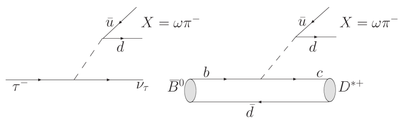
Figure 1: Feynman diagrams for $\tau\rightarrow\omega\pi\nu$ and $\kern 1.79993pt\overline{\kern-1.79993ptB}{}^{0}\rightarrow D^{*+}\omega\pi^{-}$.

In the event that $X$ is a multi-body system, it is possible that some fraction of the hadronic system could be emitted in association with the $B\rightarrow D^{(*)}$ transition instead of the hadronization from $W^{*}\rightarrow q\bar{q}^{\prime}$ decay. In the case of $X\equiv\omega\pi^{-}$, the pion must come from the $W^{*}$ to conserve charge. It is unlikely that the $\omega$ could be produced from the lower vertex in Fig. 1 LLW ; CDstOmg . Furthermore the $\omega\pi^{-}$ state is not associated with any narrow resonance, so that a wide range in $\omega\pi^{-}$ invariant mass can be studied. As the branching fraction for $\kern 1.79993pt\overline{\kern-1.79993ptB}{}^{0}\rightarrow D^{*+}\omega\pi^{-}$ is large ($\approx$ 0.3%), this decay provides a good laboratory for the study of factorization.

The branching fraction for $\kern 1.79993pt\overline{\kern-1.79993ptB}{}^{0}\rightarrow D^{*+}\omega\pi^{-}$ has been measured by the CLEO collaboration, using a sample of 9.7 million $B\bar{B}$ pairs collected at the $\mathchar 28935\relax{(4S)}$ resonance, to be $(2.9\pm 0.3{\rm(stat.)}\pm 0.4{\rm(syst.)})\times 10^{-3}$ CLEO . They also extracted the spectrum of $m_{X}^{2}$, the square of the invariant mass of the $\omega\pi$ system. This spectrum is found to be in agreement with theoretical expectations LLW . In addition, the CLEO collaboration studied the related decay $B\rightarrow D\omega\pi$ and concluded that this decay is dominated by the broad $\rho(1450)$ intermediate resonance; i.e., $B\rightarrow D\rho(1450)$, $\rho(1450)\rightarrow\omega\pi$. Assuming that this intermediate state also dominates in $\kern 1.79993pt\overline{\kern-1.79993ptB}{}^{0}\rightarrow D^{*+}\omega\pi^{-}$, factorization can be used to predict the polarization of the $D^{*}$ with the aid of heavy-quark effective theory (HQET) and data from semileptonic $B$-decays neubert . These predictions are in agreement with the CLEO result for the longitudinal polarization fraction, $\Gamma_{L}/\Gamma=(63\pm 9)$% CLEO .

In this paper we study the decay $\kern 1.79993pt\overline{\kern-1.79993ptB}{}^{0}\rightarrow D^{*+}\omega\pi^{-}$ with a larger sample of $B$ decays than available in the original CLEO study. We present measurements of the branching fraction, the Dalitz plot distribution, the $m_{X}^{2}$ spectrum, the $m_{D^{*}\pi}$ distribution, and the $D^{*}$ polarization as a function of $m_{X}$.

II The BABAR Dataset and Detector

The results presented in this paper are based on $232\times 10^{6}$ $\mathchar 28935\relax{(4S)}\rightarrow B\kern 1.79993pt\overline{\kern-1.79993ptB}{}$ decays, corresponding to an integrated luminosity of 211 fb^-1. The data were collected between 1999 and 2004 with the BABAR detector babar at the PEP-II $B$ Factory at SLAC. In addition a 22 fb^-1 off-resonance data sample, with center-of-mass energy 40 MeV below the $\mathchar 28935\relax{(4S)}$ resonance, is used to study backgrounds from continuum events, $e^{+}e^{-}\rightarrow q\bar{q}$ ($q=u,d,s,$ or $c$).

Charged-particle tracking is provided by a five-layer double-sided silicon vertex tracker (SVT) and a 40-layer drift chamber (DCH), operating within a 1.5-T magnetic field. Energy depositions are measured with a CsI(Tl) electromagnetic calorimeter (EMC). Charged particles are identified from ionization energy loss (d$E$/d$x$) measurements in the SVT and DCH, and from the observed pattern of Cherenkov light in an internally reflecting ring imaging detector.

III Analysis Strategy

Starting from the set of reconstructed charged tracks and energy deposits within the EMC, we select events that are kinematically consistent with $\kern 1.79993pt\overline{\kern-1.79993ptB}{}^{0}\rightarrow D^{*+}\omega\pi^{-}$ in the following decay modes: $D^{*+}\rightarrow D^{0}\pi^{+}$, with $D^{0}\rightarrow K^{-}\pi^{+}$, $K^{-}\pi^{+}\pi^{+}\pi^{-}$, or $K^{-}\pi^{+}\pi^{0}$, and $\omega\rightarrow\pi^{+}\pi^{-}\pi^{0}$. Charge-conjugate modes are implied throughout this paper.

In the reconstruction chain, the invariant mass requirement on the $\pi^{+}\pi^{-}\pi^{0}$ system that forms the $\omega$ candidate is kept loose. We then select “signal” or “sideband” candidates depending on whether the reconstructed $\pi^{+}\pi^{-}\pi^{0}$ mass is consistent with the $\omega$ hypothesis. Kinematic distributions of interest, such as the $m_{X}^{2}$ spectrum, are obtained by subtracting, with appropriate weights, the distributions for signal and sideband events. This subtraction accounts for all sources of backgrounds, including backgrounds from $\kern 1.79993pt\overline{\kern-1.79993ptB}{}^{0}\rightarrow D^{*+}\pi^{-}\pi^{+}\pi^{-}\pi^{0}$, on a statistical basis. This is because, as we will demonstrate in Section VI, background sources with real $\omega$ decays are negligible.

The event reconstruction efficiency is determined from simulated Monte Carlo events, where the response of the BABAR detector is modeled using the GEANT4 GEANT program. Efficiency-corrected kinematic distributions are obtained by assigning a weight to each event. This weight is equal to the inverse of the efficiency to reconstruct that particular event given its kinematic properties. This procedure, which is independent of assumptions on the dynamics of the $\kern 1.79993pt\overline{\kern-1.79993ptB}{}^{0}\rightarrow D^{*+}\omega\pi^{-}$ decay, is discussed in Section VII.

IV Event Selection Criteria

The event selection criteria are optimized based on studies of off-resonance data, and simulated $B\bar{B}$ and continuum events.

Photon candidates are constructed from calorimeter clusters with lateral profiles consistent with photon showers and with energies above 30 MeV. Neutral pion candidates are formed from pairs of photon candidates with invariant mass between 115 and 150 MeV and energy above 200 MeV, where the $\pi^{0}$ mass resolution is 6.5 MeV. In order to improve resolution, $\pi^{0}\rightarrow\gamma\gamma$ candidates are constrained to the world average $\pi^{0}$ mass PDG .

The kaon-candidate track used to reconstruct the $D^{0}$ meson must satisfy a set of kaon identification criteria. The kaon identification efficiency depends on momentum and polar angle, and is typically about 93%. These requirements provide a rejection factor of order 10 against pions. For each $D^{0}\rightarrow K^{-}\pi^{+}\pi^{0}$ candidate, we calculate the square of the decay amplitude ($|A|^{2}$) based on the kinematics of the decay products and the known properties of the Dalitz plot for this decay dalitz . We retain candidates if $|A|^{2}$ is greater than 2% of its maximum possible value. The efficiency of this requirement is 91%. Finally, the measured invariant mass of $D^{0}$ candidates must be within 15 MeV of the world average $D^{0}$ mass PDG for $D^{0}\rightarrow K^{-}\pi^{+}$ and $D^{0}\rightarrow K^{-}\pi^{+}\pi^{-}\pi^{-}$, and 25 MeV for $D^{0}\rightarrow K^{-}\pi^{+}\pi^{0}$. The experimental resolution is about 6 MeV for $D^{0}\rightarrow K^{-}\pi^{+}$, $K^{-}\pi^{+}\pi^{-}\pi^{-}$, and 10 MeV for $D^{0}\rightarrow K^{-}\pi^{+}\pi^{0}$.

We select $D^{*+}$ candidates by combining $D^{0}$ candidates with an additional track, assumed to correspond to a pion. We require the measured mass difference $\Delta m\equiv m(D^{*+})-m(D^{0})$ to be between 143.4 and 147.4 MeV. The resolution on this quantity is 0.3 MeV with non-Gaussian behavior due to the reconstruction of the low momentum pion from $D^{*}$ decay.

In the rest frame of the $\kern 1.79993pt\overline{\kern-1.79993ptB}{}^{0}$, as $m_{X}^{2}$ increases the $D^{*+}$ is produced with decreasing energy. At high $m_{X}^{2}$, or equivalently low $D^{*+}$ energy, the reconstruction efficiency drops as $\cos\theta_{D}\rightarrow 1$, where $\theta_{D}$ is the angle between the daughter $D^{0}$ and the direction opposite the flight of the $\kern 1.79993pt\overline{\kern-1.79993ptB}{}^{0}$ in the $D^{*+}$ rest frame. We exclude the region of low acceptance ($\cos\theta_{D}>0.8$ for $8\leq m_{X}^{2}<9$ GeV², $\cos\theta_{D}>0.6$ for $9\leq m_{X}^{2}<10$ GeV², and $\cos\theta_{D}>0.4$ for $m_{X}^{2}\geq 10$ GeV²) from our event selection. The effect on the final results is very small, as will be discussed in Section VIII.

We form $\omega$ candidates from a pair of oppositely-charged tracks, assumed to be a $\pi^{+}\pi^{-}$ pair, and a $\pi^{0}$ candidate. In order to keep signal and sideband candidates (see Section III) we impose only the very loose requirement that the invariant mass of the $\omega$ candidate be within 70 MeV of the world average $\omega$ mass PDG . (The natural width of the $\omega$ resonance is 8.5 MeV and the experimental resolution is 5.6 MeV.)

In order to reduce combinatoric backgrounds, we impose a requirement on the kinematics of the $\omega$ decay Perkins . This is done by first defining two Dalitz plot coordinates: $X\equiv 3T_{0}/Q-1$ and $Y\equiv\sqrt{3}(T_{+}-T_{-})/Q$, where $T_{\pm,0}$ are the kinetic energies of the pions in the $\omega$ rest frame and $Q\equiv T_{+}+T_{-}+T_{0}$. Next, we define the normalized square of the distance from the center of the Dalitz plot, $R^{2}\equiv(X^{2}+Y^{2})/(X_{b}^{2}+Y_{b}^{2})$, where $X_{b}$ and $Y_{b}$ are the coordinates of the intersection between the kinematic boundary of the Dalitz plot and a line passing through $(0,0)$ and $(X,Y)$. Since the Dalitz plot density for real $\omega$ decays peaks at $R=0$, we impose the requirement $R<0.85$. This requirement is 93% efficient for signal and rejects 25% of the combinatorial background.

We reconstruct a $B$-meson candidate by combining a $D^{*+}$ candidate, an $\omega$ candidate, and an additional negatively charged track. A $B$-candidate is characterized kinematically by the energy-substituted mass $\mbox{$m_{\rm ES}$}\equiv\sqrt{(\frac{1}{2}s+\vec{p}_{0}\cdot\vec{p}_{B})^{2}/E_{0}^{2}-p_{B}^{2}}$, where $E$ and $p$ denote energy and momentum measured in the lab frame, the subscripts $0$ and $B$ refer to the initial $\mathchar 28935\relax{(4S)}$ and $B$ candidate, respectively, and $s$ represents the square of the energy of the $e^{+}e^{-}$ center of mass (CM) system. For signal events we expect $\mbox{$m_{\rm ES}$}\approx M_{B}$ within the experimental resolution of about 3 MeV, where $M_{B}$ is the world average $B$ mass PDG . In the same fashion, the energy difference $\Delta E\equiv E_{B}^{*}-\frac{1}{2}\sqrt{s}$, where the asterisk denotes the CM frame, is expected to be nearly zero for signal $B$ decays.

The $\Delta E$ resolution is approximately 25 MeV in the $K^{-}\pi^{+}\pi^{0}$ mode and 20 MeV in the other modes, with non-Gaussian tails towards negative values due to energy leakage in the EMC. We select $B$ candidates with a $D^{0}\rightarrow K^{-}\pi^{+}\pi^{0}$ as long as $-70\leq\Delta E\leq 40$ MeV, and we require $-50\leq\Delta E\leq 35$ MeV for the other modes.

In order to further reduce the number of events from continuum backgrounds we make two additional requirements. First, we require $|\cos\theta_{B}|<0.9$, where $\theta_{B}$ is the decay angle of the $B$ candidate with respect to the $e^{-}$ beam direction in the CM frame. For real $B$ candidates, $\cos\theta_{B}$ follows a $1-x^{2}$ distribution, while the distribution is essentially flat for $B$ candidates formed from random combinations of tracks. Second, we impose a requirement on a Fisher discriminant Fisher designed to differentiate between spherical $B\bar{B}$ events and jet-like continuum events. This discriminant is constructed from the quantities $L_{0}=\sum_{i}{p^{*}_{i}}$ and $L_{2}=\sum_{i}{p^{*}_{i}\cos^{2}\alpha^{*}_{i}}$. Here, $p^{*}_{i}$ is the magnitude of the momentum and $\alpha^{*}_{i}$ is the angle with respect to the thrust axis of the $B$ candidate of tracks and clusters not used to reconstruct the $B$, all in the CM frame. The requirements on $|\cos\theta_{B}|$ and the Fisher discriminant are 95% efficient for signal and reject nearly 40% of the continuum background.

The reconstruction of the $\kern 1.79993pt\overline{\kern-1.79993ptB}{}^{0}\rightarrow D^{*+}\omega\pi^{-}$ decay is improved by refitting the momenta of the decay products of the $\kern 1.79993pt\overline{\kern-1.79993ptB}{}^{0}$, taking into account kinematic and geometric constraints. The kinematic constraints are based on the fact that their decay products must originate from a common point in space. The entire decay chain is fit simultaneously in order to account for any correlations between intermediate particles.

If more than one $B$ candidate is found in a given event with $m_{\rm ES}$ $>$ 5.2 GeV, and passes selection requirements, we retain the best candidate based on a $\chi^{2}$ algorithm that uses the measured values, world average values, and resolutions of the $D^{0}$ mass and the mass difference $\Delta m$. We omit the $\omega$ candidate mass information from arbitration in order to avoid introducing a bias in the $\omega$ mass distribution, since this distribution is used extensively throughout the analysis.

V Event yield

In Fig. 2 we show the $m_{\rm ES}$ distribution for candidates with reconstructed $\pi^{+}\pi^{-}\pi^{0}$ mass ($m_{\omega}$) in the signal and sideband regions, which are defined as $|m_{\omega}-m_{\omega}^{PDG}|<20$ MeV and $35<|m_{\omega}-m_{\omega}^{PDG}|<70$ MeV, respectively, where $m_{\omega}^{PDG}$ is the world average $\omega$ mass PDG .

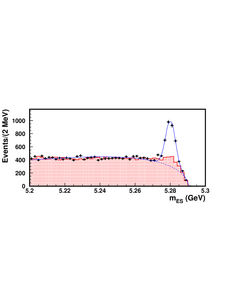
Figure 2: $m_{\rm ES}$ distributions for candidates with reconstructed $\omega$ mass in the signal (points) and sideband (shaded histogram) regions. The distribution for events in the sideband region has been rescaled to match the expected background in the $m_{\omega}$ signal region. The fitted function is described in the text.

The $m_{\rm ES}$ distribution for the $m_{\omega}$ signal region has been fitted to the sum of a threshold background function ARGUS and a Gaussian distribution centered at $M_{B}$. The distribution for the $m_{\omega}$ sideband region demonstrates the presence of a background component, which peaks in $m_{\rm ES}$ but not in $m_{\omega}$, that is not well described by the threshold function. Monte Carlo studies indicate that approximately one-third of this component is due to signal events where the $\omega$ is mis-reconstructed. These are, for example, events where one of the pion tracks in the $\omega$ decay is lost and is replaced by a track from the decay of the other $B$ in the event. The remaining two-thirds of the $m_{\rm ES}$ peaking background component is due to $\kern 1.79993pt\overline{\kern-1.79993ptB}{}^{0}\rightarrow D^{*+}\pi^{+}\pi^{-}\pi^{0}\pi^{-}$ events.

We extract the event yield from a binned $\chi^{2}$ fit of the $m_{\omega}$ distribution for events with $m_{\rm ES}$ $>$ 5.27 GeV. The data distribution is modelled as the sum of a Voigtian function and a linear background function. (The Voigtian is the convolution of a Breit-Wigner with a Gaussian resolution function.) The width of the Breit-Wigner is fixed at 8.5 MeV, the world average width of the $\omega$. The mass of the $\omega$, the Gaussian resolution term, and the parameters of the linear function are free in the fit.

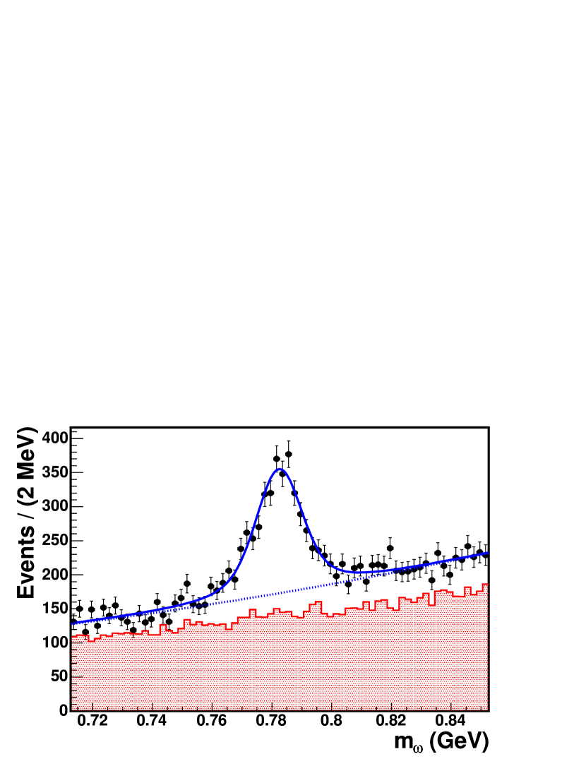
Figure 3: Distribution of reconstructed $m_{\omega}$ for events with $\mbox{$m_{\rm ES}$}>5.27$ GeV (points) and events with $5.20<\mbox{$m_{\rm ES}$}<5.25$ GeV (shaded histogram). The superimposed fit is described in the text. The events from the $m_{\rm ES}$ sideband have been scaled to the expected background from an $m_{\rm ES}$ fit to events with $|m_{\omega}-m_{\omega}^{PDG}|<70$ MeV (i.e., the range shown in this figure).

The $m_{\omega}$ distribution and the associated fit is shown in Fig. 3. The yield, defined as the number of events in the Voigtian with $|m_{\omega}-m_{\omega}^{PDG}|<20$ MeV, is $1799\pm 87$ events. The Gaussian resolution returned by the fit as well as the mean of the Breit-Wigner are consistent with the value we find in Monte Carlo simulations of $\kern 1.79993pt\overline{\kern-1.79993ptB}{}^{0}\rightarrow D^{*+}\omega\pi^{-}$ events. In Fig. 3 we also include the $m_{\omega}$ distribution for events with $5.20<\mbox{$m_{\rm ES}$}\ <5.25$ GeV (the $m_{\rm ES}$ sideband). This background distribution has been scaled to the number of background events expected from a fit to the $m_{\rm ES}$ distribution where we require $|m_{\omega}-m_{\omega}^{PDG}|<70$ MeV. The difference between the number of observed events away from the $m_{\omega}$ peak and the number of background events predicted from the $m_{\rm ES}$ sideband is due to the background component that peaks in $m_{\rm ES}$.

The validity of the yield extraction relies on the assumption that the background is linear in $m_{\omega}$, and, most importantly, that there are no sources of combinatoric backgrounds that include real $\omega$ decays. The results shown in Fig. 3 imply that there is no significant component of real $\omega$ decays in the background. To verify this, we have examined and fit the $m_{\omega}$ distribution for data events in the $m_{\rm ES}$ sideband as well as the distribution for Monte Carlo simulations of $B\bar{B}$ events, excluding $\kern 1.79993pt\overline{\kern-1.79993ptB}{}^{0}\rightarrow D^{*+}\omega\pi^{-}$. We find that the distributions are well modelled by linear functions. There is no evidence of a real $\omega$ component in the background. We estimate that this component can affect the yield extraction of Fig. 3 at most at the few percent level.

We also divide our dataset into three independent sub-datasets, according to the three $D^{0}$ decay modes that we consider. The fits to these sub-datasets yield consistent results.

VI Background Subtraction

In this work we are interested in studying a number of kinematic distributions for $\kern 1.79993pt\overline{\kern-1.79993ptB}{}^{0}\rightarrow D^{*+}\omega\pi^{-}$, such as the $m^{2}_{X}$ distribution, where $m_{X}$ is the invariant mass of the $\omega\pi$ system. The measurements of these distributions need to account for the presence of background in the sample and for the fact that the signal reconstruction efficiency is not constant over the Dalitz plot.

We use distributions for $\omega$ sideband events to remove the effects of the background in the $\omega$ signal region on a statistical basis, and we use Monte Carlo simulations to correct for efficiency effects. This is accomplished as follows:

1. The simulation of $\kern 1.79993pt\overline{\kern-1.79993ptB}{}^{0}\rightarrow D^{*+}\omega\pi^{-}$ events is used to calculate the signal reconstruction efficiency $\epsilon(\vec{x})$, where $\vec{x}$ is the set of quantities that specify the kinematics of a given event. The procedure used to determine $\epsilon(\vec{x})$ is discussed in Section VII.

2. In the absence of background, we would calculate the number of events corrected for efficiency in a given bin of $m^{2}_{X}$ as

   $$N(m^{2}_{X})=\sum_{\rm signal}\frac{1}{\epsilon(\vec{x}_{i})},$$ (1)

   where the sum is over signal events in a given $m^{2}_{X}$ bin and $\vec{x}_{i}$ is the set of kinematic quantities for the $i$-th event in the sum.

3. As mentioned above, the background subtraction is performed using the $m_{\omega}$ sideband. Thus, Eq. 1 is modified to be

   $$N(m^{2}_{X})=\sum_{\rm signal}\frac{1}{\epsilon(\vec{x}_{i})}~{}~{}-~{}~{}\frac{4}{7}\beta\sum_{\rm sideband}\frac{1}{\epsilon(\vec{x}_{j})}$$ (2)

   where the first sum is just as before, while the second sum is over $\omega$-mass sideband events in the given bin of $m_{X}^{2}$ and $\vec{x}_{j}$ represents the set of kinematic quantities for the $j$-th event in the sideband event sample. The same efficiency is used for both the signal and sideband event samples. The factor of $\frac{4}{7}$ is needed to adjust for the relative size of the $\omega$ signal and sideband regions. The additional factor of $\beta$ is ideally equal to one, and it is introduced to correct for any possible bias in the background subtraction procedure, as will be discussed below.

The allowed kinematic limits for some variables, such as $m^{2}_{X}$, are not the same for $\omega$ signal and sideband events. Therefore, the values of these variables for events in the $\omega$ sideband region are linearly rescaled so that their kinematic limits match the kinematic limits for events in the $\omega$ signal region. This procedure is necessary to avoid the introduction of artificial structures in background-subtracted distributions for these variables near the kinematic limits.

We test the sideband subtraction algorithm on a number of background samples such as Monte Carlo $B\bar{B}$ events and data events in sidebands of $m_{\rm ES}$ and $\Delta E$. These tests are performed using the efficiency parametrization discussed in Section VII. We find that background-subtracted kinematic distributions in the background samples show no significant structure. One sample distribution is shown in Fig. 4. We find a small bias in the extraction of the background-subtracted yields if the parameter $\beta$ in Eq. 2 is set to unity. To correct for this bias we set $\beta=0.975$, with an estimated systematic uncertainty of $\pm 0.010$.

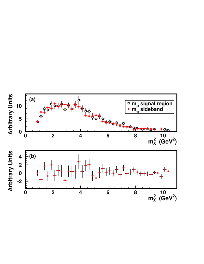
Figure 4: (a) Efficiency-corrected $m^{2}_{X}$ distributions for events from the $m_{ES}$ sideband with reconstructed $m_{\omega}$ in the signal and sideband regions (arbitrary units). The distribution for events in the sideband region has been scaled by a factor of $\frac{4}{7}$. (b) Background subtracted $m^{2}_{X}$ distribution for events from the $m_{ES}$ sideband (arbitrary units). This distribution has been obtained by subtracting the two distributions in (a).

VII Efficiency Parametrization

The process of interest ($\kern 1.79993pt\overline{\kern-1.79993ptB}{}^{0}\rightarrow D^{*+}\omega\pi^{-}$) is the three-body decay of a pseudoscalar particle into two vector particles and a pseudoscalar particle. We parametrize the reconstruction efficiency as a function of five variables:

1. $d$, an index that labels the decay mode of the $D^{0}$; i.e., $D^{0}\rightarrow K^{-}\pi^{+}$, $K^{-}\pi^{+}\pi^{+}\pi^{-}$, or $K^{-}\pi^{+}\pi^{0}$;

2. $E_{\omega}$, the energy of the $\omega$ in the $\kern 1.79993pt\overline{\kern-1.79993ptB}{}^{0}$ rest frame;

3. $E_{D^{*}}$, the energy of the $D^{*}$ in the $\kern 1.79993pt\overline{\kern-1.79993ptB}{}^{0}$ rest frame;

4. $\cos\theta_{D}$, the cosine of the decay angle of the $D^{*}$; i.e., the angle between the $D^{0}$ and the direction opposite the flight of the $\kern 1.79993pt\overline{\kern-1.79993ptB}{}^{0}$ in the $D^{*+}$ rest frame.

5. $\cos\alpha$, the cosine of the angle between the vector normal to the $\omega$ decay plane and the direction opposite the flight of the $\kern 1.79993pt\overline{\kern-1.79993ptB}{}^{0}$, measured in the $\omega$ rest frame.

Note that two other variables would be needed to fully describe the kinematics of the decay chain. These are the angles that define, in addition to $\cos\theta_{D}$ and $\cos\alpha$, the orientation between the decay planes of the $D^{*}$ and the $\omega$ and the decay plane of the $\kern 1.79993pt\overline{\kern-1.79993ptB}{}^{0}$. Monte Carlo studies show that the reconstruction efficiency is independent of these two variables. The $E_{\omega}$ and $E_{D^{*}}$ variables are the usual Dalitz variables used to describe three-body decays. Because of energy-momentum conservation the $E_{\omega}$ and $E_{D^{*}}$ variables are equivalent in information content to the squared invariant masses of the $D^{*}\pi$ ($m^{2}_{D^{*}\pi}$) and $\omega\pi$ ($m^{2}_{X}$) systems respectively.

The efficiency is then parametrized as

$$\epsilon(\vec{x}_{i}) = \epsilon(E_{\omega},E_{D^{*}},\cos\theta_{D},|\cos\alpha|;d)$$

$$= \epsilon^{\prime}(E_{\omega},E_{D^{*}};d)\cdot c_{1}(E_{\omega},|\cos\alpha|)\cdot c_{2}(E_{D^{*}},\cos\theta_{D};d).$$

The functions $\epsilon^{\prime}$, $c_{1}$, and $c_{2}$ are extracted from Monte Carlo simulations and tabulated as a set of two dimensional histograms. As an example, the $\epsilon^{\prime}$ distribution for events with $D^{0}\rightarrow K^{-}\pi^{+}$ is given in Fig. 5.

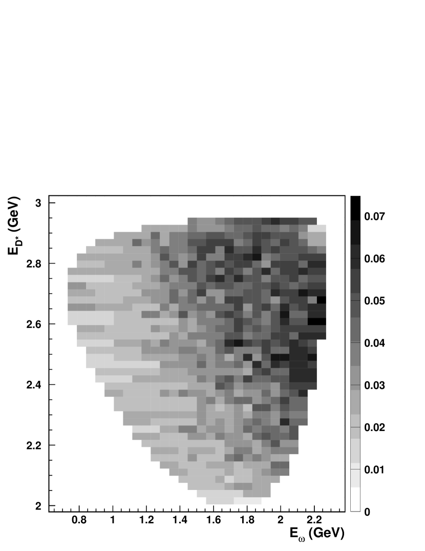
Figure 5: The $\epsilon^{\prime}$($D^{0}\rightarrow K^{-}\pi^{+}$, $E_{\omega}$, $E_{D^{*}}$) distribution for $\kern 1.79993pt\overline{\kern-1.79993ptB}{}^{0}\rightarrow D^{*+}\omega\pi^{-}$ Monte Carlo events.

The efficiency parametrization is validated using samples of Monte Carlo signal events. These samples are generated with a variety of ad-hoc kinematic properties; e.g., different polarizations for the $D^{*}$ and the $\omega$, different shapes of the $m_{X}^{2}$ distribution. In all cases we find that the shapes of kinematic distributions are well reproduced after the efficiency correction.

We use the following method to estimate the effect of the finite statistics of the Monte Carlo sample. We generate a set of 400 new $\epsilon^{\prime}$, $c_{1}$, and $c_{2}$ templates based on the nominal templates obtained from Monte Carlo signal events. If the measured efficiency in a given bin of the nominal template is $\mu\pm\sigma$, the corresponding efficiencies in the new templates are drawn from a Gaussian distribution of mean $\mu$ and standard deviation $\sigma$. Then, the measurement of any quantity of interest (e.g., $m_{X}^{2}$) is repeated 400 times, according to Eq. 2, using the new templates. The spread in the results obtained from events reconstructed in data is a measure of the systematic uncertainty due to the finite number of available Monte Carlo events. This spread is then added in quadrature to the statistical uncertainty of our results.

We observe a small bias in the total number of reconstructed signal events obtained from the efficiency correction. This is due to the fact that, although the uncertainty on $\epsilon(\vec{x}_{i})$ is Gaussian, the factor $1/\epsilon(\vec{x}_{i})$ used in the efficiency correction procedure (Eqs. 1, 2) does not obey Gaussian statistics. As a result, after applying the efficiency correction, the total number of reconstructed events tends to slightly overestimate the true value.

In order to quantify this bias on the nominal result due to the finite number of Monte Carlo signal events, we first determine the mean of the total number of reconstructed signal events in data for the 400 new efficiency templates. This mean differs from the nominal result by a few percent ($\delta$). We then repeat the procedure described above using events reconstructed from signal Monte Carlo. We use the results of these Monte Carlo studies to describe the bias as a function of $\delta$. We find that after applying the efficiency correction and subtracting the $m_{\omega}$ sideband, the total number of events reconstructed using signal Monte Carlo exceeds the true value by $(0.6\pm 0.4)\cdot\delta$. We correct our final results by this amount.

VIII Results

We use the procedure outlined above, with one additional correction, to extract the branching fraction, the $m_{X}^{2}$ distribution, the Dalitz plot distribution, the $m_{D^{*}\pi}$ distribution, and the polarization of the $D^{*}$ as a function of $m_{X}$. The one additional correction accounts for the region of phase space with low acceptance that was excluded from the analysis. This region corresponds to values of $\cos\theta_{D}$ near 1 for low $E_{D}^{*}$, or equivalently high $m_{X}^{2}$. This correction factor varies between approximately 1.2 at $m_{X}^{2}=8$ GeV² and 1.6 at $m_{X}^{2}=11$ GeV². Since most of the data is at $m_{X}^{2}<4$ GeV², the combined effect of this correction is quite small; it amounts to an increase of less than 1% relative to the measured branching fraction.

For the branching fraction, we find ${\cal B}(\kern 1.79993pt\overline{\kern-1.79993ptB}{}^{0}\rightarrow D^{*+}\omega\pi^{-})=(2.88\pm 0.21{\rm(stat.)}\pm 0.31{\rm(syst.)})\times 10^{-3}$. The total systematic uncertainty of 10.8% arises from the following sources:

• The uncertainties in the branching fractions of the $D^{*}$, $D$, and $\omega$: 5%.

• The uncertainty in the reconstruction efficiency of neutral pions at BABAR, which is estimated to be 3% per $\pi^{0}$. This amounts to a 6% uncertainty for events reconstructed with $D^{0}\rightarrow K^{-}\pi^{+}\pi^{0}$, and 3% for the other modes. Combining these modes, the systematic uncertainty from this source is 4.3%.

• The uncertainty in the reconstruction efficiency for charged tracks. From a variety of control samples, this is estimated to be 0.6% (0.8%) for each track of transverse momentum above (below) 200 MeV. Including the uncertainty for the low momentum pion produced in the $D^{*+}$ decay, we obtain a systematic uncertainty of 5.3%.

• The uncertainty in the efficiency of the kaon particle identification requirements: 2%.

• The uncertainty due to the limited Monte Carlo sample size in the efficiency calculation: 3.8%.

• The uncertainty on the quantity $\beta$ in Eq. 2: 2.6%.

• The uncertainty in the efficiency of the various event selection criteria, estimated to be 4.3%.

• The uncertainty in the number of $B\bar{B}$ events in the BABAR event sample: 1.1%.

• The uncertainty in the correction due to the removal of events at high $\cos\theta_{D}$ and small $E_{D^{*}}$: 0.3%.

Some of these systematic uncertainties vary as a function of $m_{X}^{2}$. For example, the uncertainty on the correction due to removing a region of $(E_{D^{*}},\cos\theta_{D})$ phase space is only relevant to events with $m_{X}^{2}$ above 8 GeV². A portion of the systematic uncertainty due to limited Monte Carlo sample size also varies as a function of $m_{X}^{2}$. Therefore, quantities measured as a function of $m_{X}^{2}$ include a common scale uncertainty of 10.5% and a systematic uncertainty that varies with $m_{X}^{2}$ and is typically below a few percent.

The $m^{2}_{X}$ distribution, normalized to the semileptonic width $\Gamma(B\rightarrow D^{*}\ell\nu)$ PDG , is shown in Fig. 6. A scale uncertainty on our result of 11.3% is not shown. This uncertainty combines a 4.2% uncertainty in $\Gamma(B\rightarrow D^{*}\ell\nu)$ with the 10.5% uncertainty from the sources listed above. The bulk of the data is concentrated in a broad peak around $m_{X}^{2}\approx 2$ GeV², in the region of $\rho(1450)\rightarrow\omega\pi$. Our distribution agrees well in both shape and normalization with predictions based on factorization and $\tau$ decay data CLEOtau in the region $m_{X}^{2}\leq 2.8$ GeV² covered by the tau data.

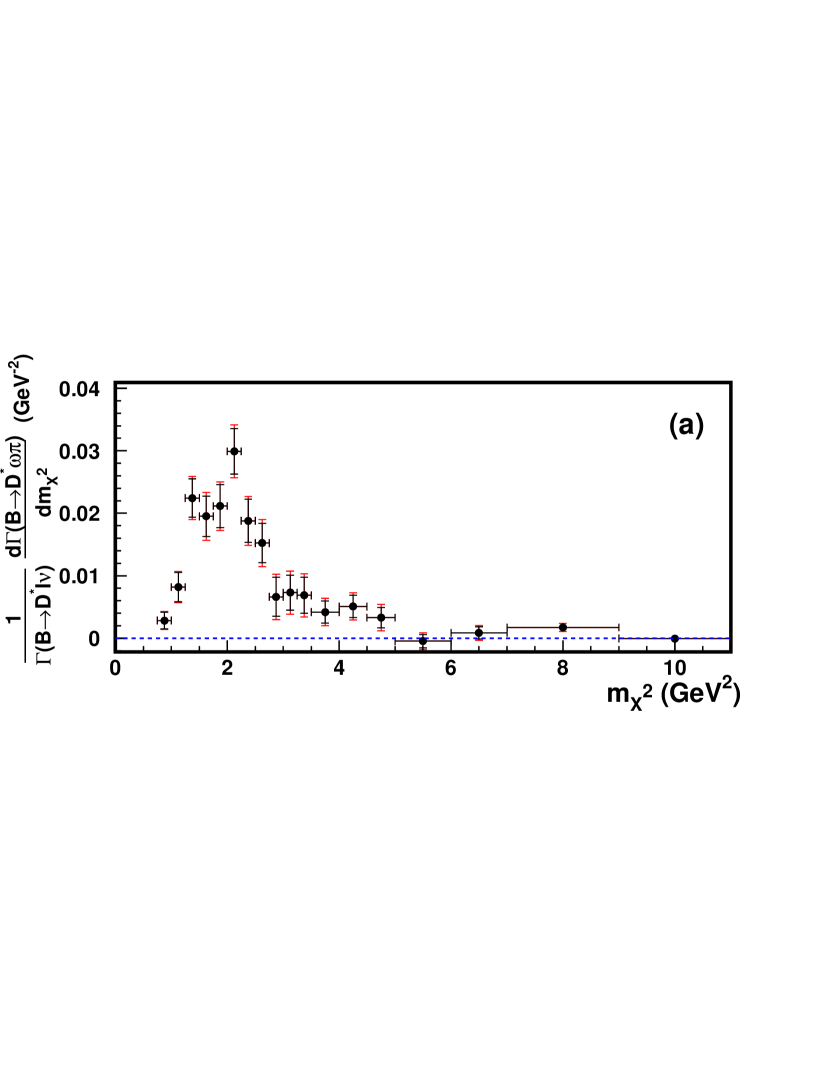
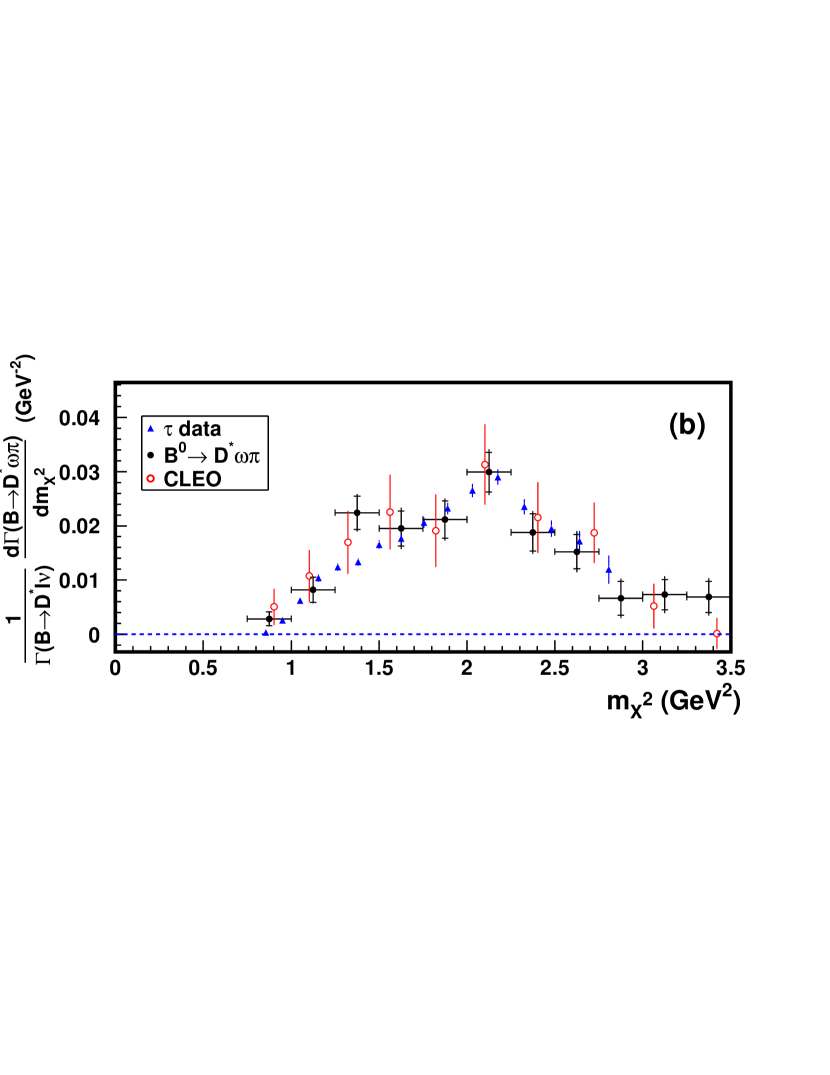
Figure 6: (a) Data $m_{X}^{2}$ distribution normalized to the semileptonic width $\Gamma(B\rightarrow D^{*}\ell\nu)$. The inner error bars reflect the statistical uncertainties on the data. The total error bars include the $m_{X}^{2}$-dependent systematic uncertainties. A common 11.3% scale systematic uncertainty is not shown. (b) Same as (a) but zoomed-in on the low $m_{X}^{2}$ region, where comparisons based on factorization and $\tau$ data can be made. Also shown here are the results from the CLEO analysis CLEO .

The background-subtracted and efficiency-corrected Dalitz plot is shown in Fig. 7. One notable feature of the decay distribution is an enhancement for $D^{*}\pi$ masses near 2.5 GeV ($m^{2}_{D^{*}\pi}\sim 6.3$ GeV²). The enhancement occurs in the region where one expects to find a broad $J=1$ $D^{**}$ resonance ($D^{\prime}_{1}$) that decays via S-wave to $D^{*}\pi$. Thus, this enhancement could be due to the color-suppressed decay $\kern 1.79993pt\overline{\kern-1.79993ptB}{}^{0}\rightarrow D^{\prime}_{1}\omega$, followed by $D^{\prime}_{1}\rightarrow D^{*+}\pi^{-}$.

Figure 7: Background-subtracted and efficiency-corrected Dalitz plot for $B\rightarrow D^{*}\omega\pi$. The relative box sizes indicate the population of the bins. Black boxes indicate positive values, white boxes indicate negative values, which can occur because of statistical fluctuations in the subtraction procedure.

In Fig. 8 we show the background-subtracted and efficiency-corrected $D^{*}\pi$ mass distribution for events away from the $\rho(1450)$ peak, fitted to the sum of a fourth order polynomial and a relativistic Breit-Wigner. In this figure, in order to remove the contribution from the $\rho(1450)$, we have required $\cos\theta_{D^{*}}<0.5$, where $\theta_{D^{*}}$ is the angle between the momentum of the $D^{*}$ in the $D^{*}\pi$ rest frame, and the flight direction of $D^{*}\pi$ system. We use the $\cos\theta_{D^{*}}$ variable rather than $m_{X}^{2}$ to remove the $\rho(1450)$ contribution because the distribution in $\cos\theta_{D^{*}}$ is uniform for S-wave $D^{\prime}_{1}\rightarrow D^{*}\pi$ decay. The yield of possible $\kern 1.79993pt\overline{\kern-1.79993ptB}{}^{0}\rightarrow D^{\prime}_{1}\omega$ events in Fig. 8 can then be easily extrapolated to the full kinematic range. Furthermore, by subdividing the dataset in bins of $\cos\theta_{D^{*}}$ we can test the S-wave decay hypothesis.

The fitted mass and width of the Breit-Wigner in Fig. 8 are $2477\pm 28$ MeV and $266\pm 97$ MeV, respectively. These values are consistent with the parameters of the broad $D^{\prime}_{1}\rightarrow D^{*}\pi$ resonance observed by the Belle collaboration in $B\rightarrow D^{\prime}_{1}\pi$ decays, $m=2427\pm 36$ MeV and $\Gamma=384^{+107}_{-75}\pm 74$ MeV Belle . We have also split the data set of Fig. 8 into three equal-sized bins of $\cos\theta_{D^{*}}$. We find that the fitted amplitude of the Breit-Wigner component is the same, within statistical uncertainties, in the three data sets. This is consistent with expectations for an S-wave $D^{\prime}_{1}\rightarrow D^{*}\pi$ decay.

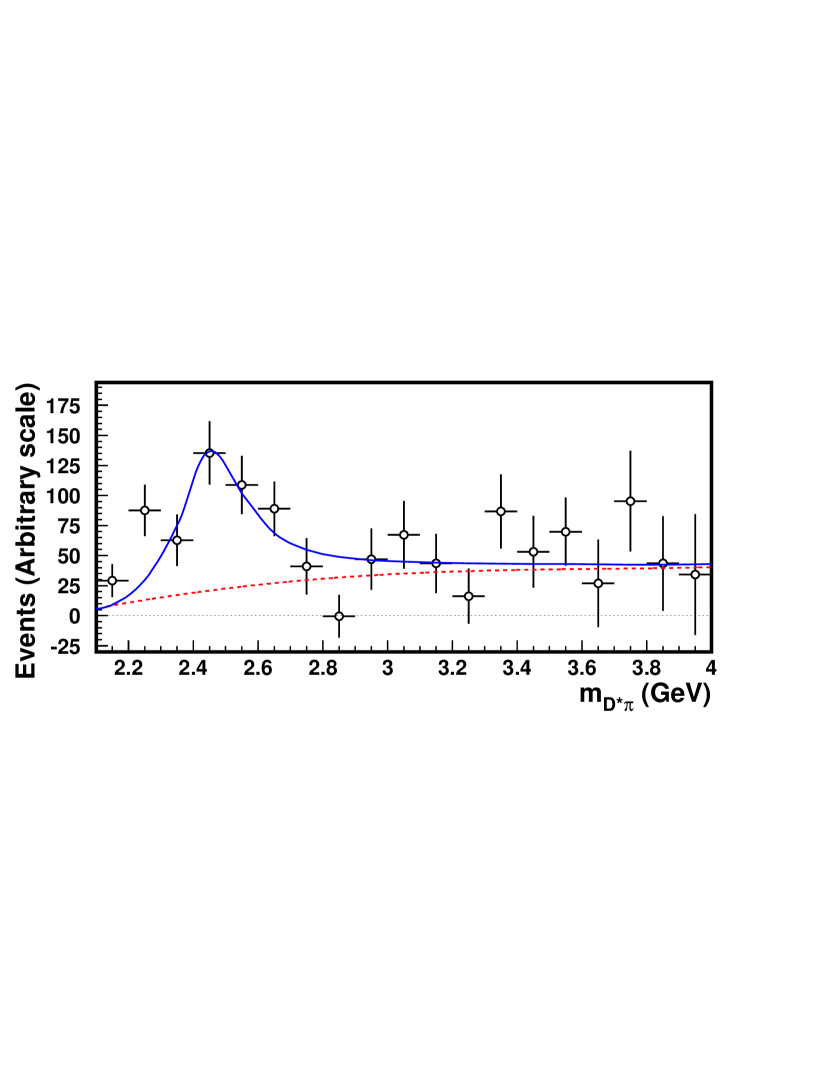
Figure 8: Background-subtracted and efficiency-corrected $D^{*}\pi$ mass distribution with $\cos\theta_{D^{*}}<0.5$. The superimposed fit is described in the text.

If we assume that the enhancement for $D^{*}\pi$ masses near 2.5 GeV is actually due to $\kern 1.79993pt\overline{\kern-1.79993ptB}{}^{0}\rightarrow D^{\prime}_{1}\omega$, $D^{\prime}_{1}\rightarrow D^{*+}\pi^{-}$, we extract the branching fraction

$${\cal B}(\kern 1.79993pt\overline{\kern-1.79993ptB}{}^{0}\rightarrow D^{\prime}_{1}\omega)\times{\cal B}(D^{\prime}_{1}\rightarrow D^{*+}\pi^{-})=$$

$$(4.1\pm 1.2\pm 0.4\pm 1.0)\times 10^{-4}.$$ (4)

In this measurement, the first uncertainty is statistical, the second uncertainty is from the uncertainties in common with the ${\cal B}(\kern 1.79993pt\overline{\kern-1.79993ptB}{}^{0}\rightarrow D^{*+}\omega\pi^{-})$ measurement, and the last uncertainty arises from the uncertainties on the choice of the nonresonant shape in Fig. 8 (10%) and the uncertainties in the parameters of the $D^{\prime}_{1}$ resonance (22%). This branching fraction has been obtained from fitting the sample of events with $\cos\theta_{D^{*}}<0.5$, and scaling up the result by a factor of $\frac{4}{3}$. This procedure neglects interference effects between $\kern 1.79993pt\overline{\kern-1.79993ptB}{}^{0}\rightarrow D^{\prime}_{1}\omega$ and $\kern 1.79993pt\overline{\kern-1.79993ptB}{}^{0}\rightarrow D^{*}\omega\pi$.

The branching fraction in Eq. 4 is comparable to the branching fractions for $\kern 1.79993pt\overline{\kern-1.79993ptB}{}^{0}\rightarrow D^{(*)0}\omega$ PDG . Also, we see no evidence for decays into the two narrow $D^{**}$ resonances at 2420 and 2460 MeV. This is in contrast to the color-favored $B^{-}\rightarrow D^{**0}\pi^{-}$ decays, where the three $D^{**}$ modes contribute with comparable strengths, and where the $B^{-}\rightarrow D^{\prime}_{1}\pi^{-}$ branching fraction is one order of magnitude smaller than that of $B^{-}\rightarrow D^{(*)0}\pi^{-}$.

The presence of $\kern 1.79993pt\overline{\kern-1.79993ptB}{}^{0}\rightarrow D^{\prime}_{1}\omega$ would affect the comparison of the data with the theoretical predictions of Fig. 6. As can be seen in Fig. 7, $\kern 1.79993pt\overline{\kern-1.79993ptB}{}^{0}\rightarrow D^{\prime}_{1}\omega$ would mostly contribute at high value of $m_{X}^{2}$, while the factorization test can be carried out only where the $\tau$ data is available; i.e., for $m_{X}^{2}<3$ GeV². Based on the estimated branching fraction of $\kern 1.79993pt\overline{\kern-1.79993ptB}{}^{0}\rightarrow D^{\prime}_{1}\omega$, and neglecting interference effects, the contribution of $\kern 1.79993pt\overline{\kern-1.79993ptB}{}^{0}\rightarrow D^{\prime}_{1}\omega$ to the $m_{X}^{2}<3$ GeV² distribution would be less than 5%.

If the decay $\kern 1.79993pt\overline{\kern-1.79993ptB}{}^{0}\rightarrow D^{*+}\omega\pi^{-}$ proceeds dominantly through $\kern 1.79993pt\overline{\kern-1.79993ptB}{}^{0}\rightarrow D^{*+}\rho(1450)$, $\rho(1450)\rightarrow\omega\pi^{-}$, a measurement of the polarization of the $D^{*}$ can provide a further test of factorization and HQET poltheory . The angular distribution in the $D^{*+}\rightarrow D^{0}\pi^{+}$ decay can be written as a function of three complex amplitudes $H_{0}$ (longitudinal), and $H_{+}$ and $H_{-}$(transverse), as

$$\frac{d\Gamma}{d\cos\theta_{D}}\propto 4|H_{0}|^{2}\cos^{2}\theta_{D}+(|H_{+}|^{2}+|H_{-}|^{2})\sin^{2}\theta_{D},$$ (5)

where $\theta_{D}$ is the decay angle of the $D^{*}$ defined above.

The longitudinal polarization fraction $\Gamma_{L}/\Gamma$, given by

$$\frac{\Gamma_{L}}{\Gamma}=\frac{|H_{0}|^{2}}{|H_{0}|^{2}+|H_{+}|^{2}+|H_{-}|^{2}},$$ (6)

can then be extracted using Eq. 5 from a fit to the angular distribution in the decay of the $D^{*}$.

We divide our dataset in ranges of $m^{2}_{X}$, and perform binned chi-squared fits to the efficiency-corrected, background-subtracted, $D^{*}$-decay angular distributions. In these measurements, nearly all of the systematic uncertainties discussed above cancel. As a result, the $m_{X}^{2}$-dependent uncertainty due to the finite Monte Carlo sample is the dominant systematic uncertainty, and typically results in an uncertainty on $\Gamma_{L}/\Gamma$ at the few percent level. We also include a systematic uncertainty due to the parameter $\beta$ in Eq. 2. This uncertainty is about one order of magnitude smaller.

The measured longitudinal polarization fractions as a function of $m_{X}$ are presented in Table I. Near the mean of the $\rho(1450)$ resonance ($1.1<m_{X}<1.9$ GeV), we find $\Gamma_{L}/\Gamma=0.654\pm 0.042{\rm(stat.)}\pm 0.016{\rm(syst.)}$. This result is in agreement with the previous result in the same mass range from the CLEO collaboration, $\Gamma_{L}/\Gamma=0.63\pm 0.09$. It is also in agreement with predictions based on HQET, factorization, and the measurement of semileptonic $B$-decay form factors, $\Gamma_{L}/\Gamma=0.684\pm 0.009$ DstlnuFF , assuming that the decay proceeds via $\kern 1.79993pt\overline{\kern-1.79993ptB}{}^{0}\rightarrow D^{*+}\rho(1450)$, $\rho(1450)\rightarrow\omega\pi^{-}$. These results are shown in Fig. 9.

Table 1: Results of the $D^{*}$ polarization measurement in bins of $m_{X}$. The first uncertainty is statistical and the second is systematic.

$m_{X}$ range (GeV)	$\Gamma_{L}/\Gamma$
below 1.1	0.458 $\pm$ 0.189 $\pm$ 0.059
1.1 - 1.35	0.779 $\pm$ 0.062 $\pm$ 0.020
1.35 - 1.55	0.733 $\pm$ 0.071 $\pm$ 0.024
1.55 - 1.9	0.435 $\pm$ 0.102 $\pm$ 0.040
1.9 - 2.83	0.656 $\pm$ 0.182 $\pm$ 0.077

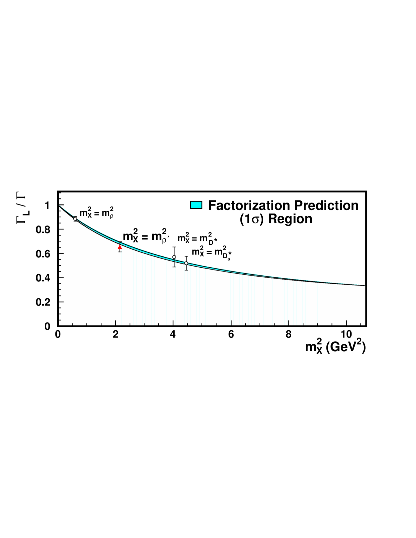
Figure 9: The fraction of longitudinal polarization as a function of $m_{X}^{2}$, where $X$ is a vector meson. Shown (as a triangle) is the $\kern 1.79993pt\overline{\kern-1.79993ptB}{}^{0}\rightarrow D^{*+}\omega\pi^{-}$ polarization measurement for events with $1.1<m_{X}<1.9$ GeV ($m_{X}^{2}$ = $m^{2}_{\rho^{\prime}}$, where $\rho^{\prime}\equiv\rho(1450)$), as well as earlier measurements (indicated by open circles) of $\kern 1.79993pt\overline{\kern-1.79993ptB}{}^{0}\rightarrow D^{*+}\rho^{-}$ DstRho , $\kern 1.79993pt\overline{\kern-1.79993ptB}{}^{0}\rightarrow D^{*+}D^{*-}$ DstDst , and $\kern 1.79993pt\overline{\kern-1.79993ptB}{}^{0}\rightarrow D^{*+}D_{s}^{*-}$ DstDSst . The shaded region represents the prediction ($\pm$ one standard deviation) based on factorization and HQET, extrapolated from the semileptonic $\kern 1.79993pt\overline{\kern-1.79993ptB}{}^{0}\rightarrow D^{*+}\ell^{-}\bar{\nu}$ form factor results DstlnuFF .

IX Conclusions

We have studied the decay $\kern 1.79993pt\overline{\kern-1.79993ptB}{}^{0}\rightarrow D^{*+}\omega\pi^{-}$ with a larger data sample than previously available. We measure the branching fraction to be ${\cal B}(\kern 1.79993pt\overline{\kern-1.79993ptB}{}^{0}\rightarrow D^{*+}\omega\pi^{-})=(2.88\pm 0.21$(stat.) $\pm 0.32$(syst.)$)\times 10^{-3}$.

The invariant mass spectrum of the $\omega\pi$ system is found to be in agreement with theoretical expectations based on factorization and $\tau$ decay data. The Dalitz plot for this mode is very non-uniform, with most of the rate at low $\omega\pi$ mass. We also find an enhancement for $D^{*}\pi$ masses broadly distributed around 2.5 GeV. This enhancement could be due to color-suppressed decays into the broad $D^{\prime}_{1}$ resonance, $\kern 1.79993pt\overline{\kern-1.79993ptB}{}^{0}\rightarrow D^{\prime}_{1}\omega$, followed by $D^{\prime}_{1}\rightarrow D^{*+}\pi^{-}$, with a branching fraction comparable to $\kern 1.79993pt\overline{\kern-1.79993ptB}{}^{0}\rightarrow D^{(*)0}\omega$.

We also measure the fraction of $D^{*}$ longitudinal polarization in this decay. In the region of $\omega\pi$ mass between 1.1 and 1.9 GeV, where one expects contributions from $\kern 1.79993pt\overline{\kern-1.79993ptB}{}^{0}\rightarrow D^{*+}\rho(1450)$, $\rho(1450)\rightarrow\omega\pi^{-}$, we find $\Gamma_{L}/\Gamma=0.654\pm 0.042{\rm(stat.)}\pm 0.016{\rm(syst.)}$, in agreement with predictions based on HQET, factorization, and the measurement of semileptonic $B$-decay form factors.

We are grateful for the extraordinary contributions of our PEP-II colleagues in achieving the excellent luminosity and machine conditions that have made this work possible. The success of this project also relies critically on the expertise and dedication of the computing organizations that support BABAR. The collaborating institutions wish to thank SLAC for its support and the kind hospitality extended to them. This work is supported by the US Department of Energy and National Science Foundation, the Natural Sciences and Engineering Research Council (Canada), Institute of High Energy Physics (China), the Commissariat à l’Energie Atomique and Institut National de Physique Nucléaire et de Physique des Particules (France), the Bundesministerium für Bildung und Forschung and Deutsche Forschungsgemeinschaft (Germany), the Istituto Nazionale di Fisica Nucleare (Italy), the Foundation for Fundamental Research on Matter (The Netherlands), the Research Council of Norway, the Ministry of Science and Technology of the Russian Federation, and the Particle Physics and Astronomy Research Council (United Kingdom). Individuals have received support from CONACyT (Mexico), the Marie-Curie Intra European Fellowship program (European Union), the A. P. Sloan Foundation, the Research Corporation, and the Alexander von Humboldt Foundation.

References

(1) J. D. Bjorken, Nucl. Phys. B Proc. Suppl. 11, 325 (1989);
M. J. Dugan and B. Grinstein, Phys Lett. B255, 583 (1991);
H. D. Politzer and M. B. Wise, Phys Lett. B257, 399 (1991).
(2) Z. Ligeti, M. B. Luke,
and M. Wise, Phys. Lett. B507, 142 (2001);
C. Reader and N. Isgur, Phys. Rev. D 47, 1007 (1993).
(3) N. Isgur, D. Scora, B. Grinstein, and M. B. Wise,
Phys. Rev. D39, 799 (1989); D. Scora and N. Isgur, Phys. Rev. D52, 2783 (1995).
(4) CLEO Collaboration, J. P. Alexander et al.,
Phys. Rev. D64, 092001 (2001).
(5)
J. Korner and G. Goldstein, Phys. Lett. B89, 105 (1979);
M. Neubert and B. Stech, in Heavy Flavors, 2nd Edition, edited
by A. J. Buras and M. Lindner, World Scientific, Singapore, 1997.
(6)BABAR Collaboration, B. Aubert et al.,
Nucl. Inst. Methods A479, 1 (2002).
(7) S. Agostinelli et al.,
Nucl. Inst. Methods A506, 250(2003).
(8) Particle Data Group, S. Eidelman et al., Phys. Lett.
B592, 1 (2004).
(9)CLEO Collaboration,
S. Kopp et al., Phys. Rev. D 63, 092001 (2001).
(10) D. H. Perkins, Introduction to High Energy Physics, 2nd Ed.
(Addison-Wesley, Reading, 1982), p.136, 1982;
B. C. Maglic et al., Phys. Rev. Lett. 7, 178 (1961).
(11) R. A. Fisher, Ann. Eugenics 7, 179 (1936);
M. G. Kendall and A. Stuart, The Advanced Theory of Statistics,
2nd Ed. (Hafner Publishing, New York, 1968), Vol. III.
(12)The function is
,
where and is a fit parameter;
ARGUS Collaboration, H. Albrecht et al.,
Z. Phys. C48, 543 (1990).
(13) CLEO collaboration, K. W. Edwards et al.,
Phys. Rev. D61, 072003 (2000).
(14) Belle Collaboration, K. Abe et al., Phys. Rev. D69, 112002 (2004).
(15) J. Körner and G. Goldstein, Phys Lett. B89, 105 (1979);
G. Kramer and W.F. Palmer, Phys. Rev. D45, 193 (1992).
(16) CLEO Collaboration, S. E. Csorna et al.,
Phys. Rev. D67, 112002 (2003).
(17) Belle Collaboration, H. Miyake et al.,
Phys. Lett. B618, 34 (2005).
(18)BABAR Collaboration, B. Aubert et al.,
Phys. Rev. D67, 092003 (2003).
(19)BABAR Collaboration, B. Aubert et al.,
submitted to Phys. Rev. D, hep-ex/0602023.