Measurements of branching fractions, rate asymmetries, and angular distributions in the rare decays $B\rightarrow K\ell^{+}\ell^{-}$ and $B\rightarrow K^{*}\ell^{+}\ell^{-}$

Abstract

We present measurements of the flavor-changing neutral current decays $B\rightarrow K\ell^{+}\ell^{-}$ and $B\rightarrow K^{*}\ell^{+}\ell^{-}$, where $\ell^{+}\ell^{-}$ is either an $e^{+}e^{-}$ or $\mu^{+}\mu^{-}$ pair. The data sample comprises $229\times 10^{6}$ $\mathchar 28935\relax{(4S)}\rightarrow B\kern 1.79993pt\overline{\kern-1.79993ptB}{}$ decays collected with the BABAR detector at the PEP-II $e^{+}e^{-}$ storage ring. Flavor-changing neutral current decays are highly suppressed in the Standard Model and their predicted properties could be significantly modified by new physics at the electroweak scale. We measure the branching fractions ${\cal B}(B\rightarrow K\ell^{+}\ell^{-})=(0.34\pm 0.07\pm 0.02)\times 10^{-6}$, ${\cal B}(B\rightarrow K^{*}\ell^{+}\ell^{-})=(0.78^{+0.19}_{-0.17}\pm 0.11)\times 10^{-6}$, the direct $C\!P$ asymmetries of these decays, and the relative abundances of decays to electrons and muons. For two regions in $\ell^{+}\ell^{-}$ mass, above and below $m_{{J\mskip-3.0mu/\mskip-2.0mu\psi\mskip 2.0mu}}$, we measure partial branching fractions and the forward-backward angular asymmetry of the lepton pair. In these same regions we also measure the $K^{*}$ longitudinal polarization in $B\rightarrow K^{*}\ell^{+}\ell^{-}$ decays. Upper limits are obtained for the lepton flavor-violating decays $B\rightarrow Ke\mu$ and $B\rightarrow K^{*}e\mu$. All measurements are consistent with Standard Model expectations.

I Introduction

The decays $B\rightarrow K^{(*)}\ell^{+}\ell^{-}$, where $\ell^{+}\ell^{-}$ is either an $e^{+}e^{-}$ or $\mu^{+}\mu^{-}$ pair and $K^{(*)}$ denotes either a kaon or the $K^{*}(892)$ meson, are manifestations of $b\rightarrow s\ell^{+}\ell^{-}$ flavor-changing neutral currents (FCNC). In the Standard Model (SM), these decays are forbidden at tree level and can only occur at greatly suppressed rates through higher-order processes. At lowest order, three amplitudes contribute: (1) a photon penguin, (2) a $Z$ penguin, and (3) a $W^{+}W^{-}$ box diagram (Figure  1). In all three, a virtual $t$ quark contribution dominates, with secondary contributions from virtual $c$ and $u$ quarks. Within the Operator Product Expansion (OPE) framework, these short-distance contributions are typically described in terms of the effective Wilson coefficients $C_{7}^{\rm eff}$, $C_{9}^{\rm eff}$, and $C_{10}^{\rm eff}$ bib:buras . Since these decays proceed via weakly-interacting particles with virtual energies near the electroweak scale, they provide a promising means to search for effects from new interactions entering with amplitudes comparable to those of the SM. Such effects are predicted in a wide variety of models  bib:chargedhiggs ; bib:susy ; bib:TheoryA ; bib:4g ; bib:lq .

Figure 1: Examples of Standard Model Feynman diagrams for the decays $B\rightarrow K^{(*)}\ell^{+}\ell^{-}$. For the photon or $Z$ penguin diagrams on the left, boson emission can occur on any of the $b$, $t$, $c$, $u$, $s$, or $W$ lines.

In the SM the $B\rightarrow K\ell^{+}\ell^{-}$ branching fraction is predicted to be roughly $0.4\times 10^{-6}$, while the $B\rightarrow K^{*}\ell^{+}\ell^{-}$ branching fraction is predicted to be about three times larger  bib:TheoryA ; bib:TheoryBa ; bib:ErratumTheoryBa ; bib:TheoryBb ; bib:TheoryBc ; bib:TheoryBd ; bib:TheoryC . The $B\rightarrow K^{*}\ell^{+}\ell^{-}$ mode receives a significant contribution from a pole in the photon penguin amplitude at low values of $q^{2}\equiv m_{\ell^{+}\ell^{-}}^{2}$, which is not present in $B\rightarrow K\ell^{+}\ell^{-}$ decays. Due to the lower mass threshold for producing an $e^{+}e^{-}$ pair, this enhances the $K^{*}e^{+}e^{-}$ final state relative to the $K^{*}\mu^{+}\mu^{-}$ state. Currently, theoretical predictions of the branching fractions have associated uncertainties of about $30\%$ due to form factors that model the hadronic effects in the $B\rightarrow K$ or $B\rightarrow K^{*}$ transition. Previous experimental measurements of the branching fractions are consistent with the range of theoretical predictions, with experimental uncertainties comparable in size to the theoretical uncertainties  bib:babarprl03 ; bib:belleprl03 .

With larger datasets, it becomes possible to measure ratios and asymmetries in the rates. These can typically be predicted more reliably than the total branching fractions. For example, the direct $C\!P$ asymmetry

$$A_{C\!P}\equiv\frac{\Gamma(\overline{B}\rightarrow\overline{K}^{(*)}\ell^{+}\ell^{-})-\Gamma(B\rightarrow K^{(*)}\ell^{+}\ell^{-})}{\Gamma(\overline{B}\rightarrow\overline{K}^{(*)}\ell^{+}\ell^{-})+\Gamma(B\rightarrow K^{(*)}\ell^{+}\ell^{-})}$$

is expected to be vanishingly small in the SM, of order $10^{-4}$ in the $B\rightarrow K^{*}\ell^{+}\ell^{-}$ mode bib:kruger01 . However it could be enhanced by new non-SM weak phases bib:krugercp . The ratio $R_{K}$, defined as

$$R_{K}\equiv\frac{\Gamma(B\rightarrow K\mu^{+}\mu^{-})}{\Gamma(B\rightarrow Ke^{+}e^{-})},$$

also has a precise SM prediction of $R_{K}=1.0000\pm 0.0001$ bib:hiller03 . In supersymmetric theories with a large ratio ($\tan\beta$) of vacuum expectation values of Higgs doublets, $R_{K}$ can be significantly enhanced. This occurs via penguin diagrams in which the $\gamma$ or $Z^{0}$ is replaced with a neutral Higgs boson that preferentially couples to the heavier muons bib:yan . In $B\rightarrow K^{*}\ell^{+}\ell^{-}$ this ratio is modified by the photon pole contribution, thus the SM prediction is $R_{K^{*}}\approx 0.75$  bib:TheoryA with an estimated uncertainty of $0.01$ bib:hiller03 if the pole region is included, or $R_{K^{*}}\approx 1.0$ if it is excluded bib:hiller03 .

Additional sensitivity to non-SM physics arises from the fact that $B\rightarrow K^{(*)}\ell^{+}\ell^{-}$ transitions are three-body decays proceeding through three different electroweak penguin amplitudes, whose relative contributions vary as a function of $q^{2}$. Measurements of partial branching fractions and angular distributions as a function of the invariant momentum transfer $q^{2}$ are therefore of particular interest. The SM predicts a distinctive pattern in the forward-backward asymmetry

$$A_{FB}(s) \equiv {\displaystyle\int_{-1}^{1}{\rm d}\cos{\theta}\;{\displaystyle{\rm d}^{2}\Gamma(B\rightarrow K^{(*)}\ell^{+}\ell^{-})\over\displaystyle{\rm d}\cos{\theta}\;{\rm d}s}\;{\rm Sign}(\cos{\theta})\over\displaystyle{\rm d}\Gamma(B\rightarrow K^{(*)}\ell^{+}\ell^{-})/{\rm d}s},$$

where $s\equiv q^{2}/m_{B}^{2}$, and $\theta$ is the angle of the lepton with respect to the flight direction of the $B$ meson, measured in the dilepton rest frame  bib:buchalla01 . In the presence of non-SM physics, the sign and magnitude of this asymmetry can be altered dramatically bib:TheoryBb ; bib:TheoryA ; bib:kruger01 . In particular, at high $q^{2}$, the sign of $A_{FB}$ is sensitive to the sign of the product of the $C_{9}^{\rm eff}$ and $C_{10}^{\rm eff}$ Wilson coefficients. The value of $A_{FB}$ in $B\rightarrow K\ell^{+}\ell^{-}$ provides an important check on this measurement, as it is expected to result in zero asymmetry for all $q^{2}$ in the SM and many non-SM scenarios. This condition can be violated in models in which new operators such as a neutral Higgs penguin contribute significantly bib:yan . However even in this case the resulting asymmetry is expected to be of order $0.01$ or less in the $B\rightarrow K\ell^{+}\ell^{-}$ mode for electron or muon final states bib:demir02 . In addition to $A_{FB}$, in $B\rightarrow K^{*}\ell^{+}\ell^{-}$ the fraction of longitudinal polarization $F_{L}$ of the $K^{*}$ can be measured from the angular distribution of its decay products. The value of $F_{L}$ measured at low $q^{2}$ is sensitive to effects from new left-handed currents with complex phases different from the SM, resulting in $C_{7}^{\rm eff}=-C_{7}(\textrm{SM})$, or effects from new right-handed currents in the photon penguin amplitude bib:krugerf0 . The predicted distributions of $A_{FB}(q^{2})$ and $F_{L}(q^{2})$ are shown for the SM and for several non-SM scenarios in Figure 2. The non-SM scenarios correspond to those studied in Refs. bib:TheoryA ; bib:TheoryBb ; bib:krugerf0 .

Finally, the lepton flavor-violating decays $B\rightarrow K^{(*)}e^{\pm}\mu^{\mp}$ can only occur at rates far below current experimental sensitivities in the context of the SM with neutrino mixing. Observation of these decays would therefore be an indication of contributions beyond the SM. For example, such decays are allowed in leptoquark models bib:lq .

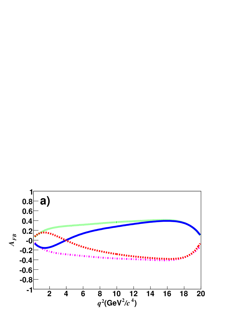
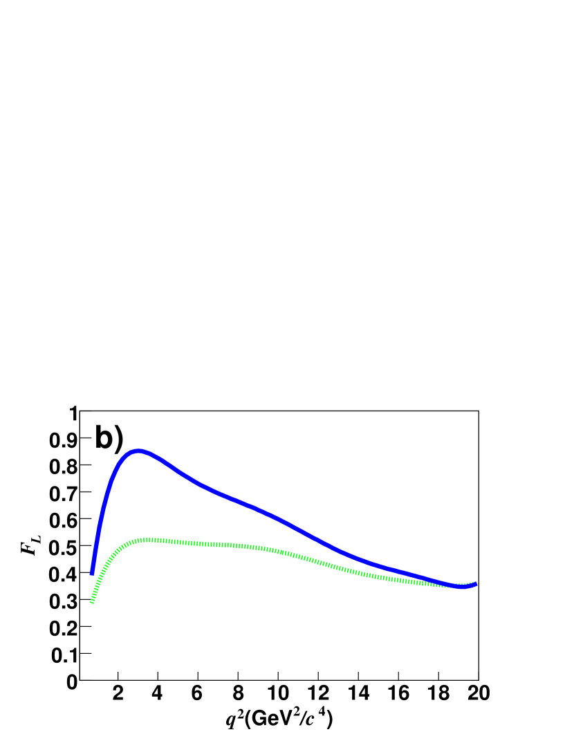
Figure 2: Simulated distribution of (a) $A_{FB}$ and (b) $F_{L}$ for the decay $B\rightarrow K^{*}\ell^{+}\ell^{-}$. The points represent the distributions assuming the SM (solid lines), $C_{7}^{\rm eff}=-C_{7}(SM)$ (dotted lines), $C_{9}^{\rm eff}C_{10}^{\rm eff}=-C_{9}C_{10}(SM)$ (dashed lines), and $C_{7}^{\rm eff},C_{9}^{\rm eff}C_{10}^{\rm eff}=-C_{7}(SM),-C_{9}C_{10}(SM)$ (dot-dashed lines) generated using the form factor model of  bib:TheoryE . In the case of $F_{L}$, the two solutions with $C_{9}^{\rm eff}C_{10}^{\rm eff}=-C_{9}C_{10}(SM)$ are not displayed; they are nearly identical to the two shown.

II Detector and dataset

The results presented here are based on data collected with the BABAR detector at the PEP-II asymmetric $e^{+}e^{-}$ collider located at the Stanford Linear Accelerator Center. The dataset comprises 229 million $B\kern 1.79993pt\overline{\kern-1.79993ptB}{}$ pairs, corresponding to an integrated luminosity of $208$ $\mbox{\,fb}^{-1}$ collected on the $\mathchar 28935\relax(4S)$ resonance at a center-of-mass energy of $\sqrt{s}=10.58$ $\mathrm{\,Ge\kern-1.00006ptV}$. An additional $12.1$ $\mbox{\,fb}^{-1}$ of data collected at energies $40$ $\mathrm{\,Me\kern-1.00006ptV}$ below the nominal on-peak energy is used to study continuum backgrounds arising from pair production of $u$, $d$, $s$, and $c$ quarks.

The BABAR detector is described in detail in Ref. bib:babarNIM . The measurements described in this paper rely primarily on the charged particle tracking and identification properties of the detector. Tracking is provided by a five-layer silicon vertex tracker (SVT) and a 40-layer drift chamber (DCH) in a $1.5$-T magnetic field produced by a superconducting magnet. Low momentum charged hadrons are identified by the ionization loss ($dE/dx$) measured in the SVT and DCH, and higher momentum hadrons by a ring-imaging detector of internally reflected Cherenkov light (DIRC). A CsI(Tl) electromagnetic calorimeter (EMC) provides identification of electrons, and detection of photons. The steel in the instrumented flux return (IFR) of the superconducting coil is interleaved with resistive plate chambers, providing identification of muons and neutral hadrons.

III Event selection

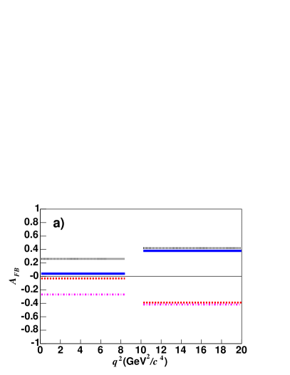
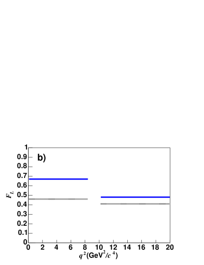
Figure 3: Predicted distributions of (a) $A_{FB}(q^{2})$ and (b) $F_{L}(q^{2})$ in $B\rightarrow K^{*}\ell^{+}\ell^{-}$ for the two regions of $q^{2}$ considered. The lines represent the predictions of the SM (solid lines), $C_{7}^{\rm eff}=-C_{7}(SM)$ (dotted lines), $C_{9}^{\rm eff}C_{10}^{\rm eff}=-C_{9}C_{10}(SM)$ (dashed lines), and $C_{7}^{\rm eff},C_{9}^{\rm eff}C_{10}^{\rm eff}=-C_{7}(SM),-C_{9}C_{10}(SM)$ (dot-dashed lines) with the form factor model of Ref. bib:TheoryE . In the case of $F_{L}$, the two solutions with $C_{9}^{\rm eff}C_{10}^{\rm eff}=-C_{9}C_{10}(SM)$ are not displayed; they are nearly identical to the two shown.

We reconstruct signal candidates in eight final states: $B^{+}\rightarrow K^{+}\ell^{+}\ell^{-}$, $B^{0}\rightarrow K^{0}_{\scriptscriptstyle S}\ell^{+}\ell^{-}$, $B^{0}\rightarrow K^{*0}\ell^{+}\ell^{-}$, $B^{+}\rightarrow K^{*+}\ell^{+}\ell^{-}$, where $K^{*0}\rightarrow K^{+}\pi^{-}$, $K^{*+}\rightarrow K_{\scriptscriptstyle S}^{0}\pi^{+}$, $K_{\scriptscriptstyle S}^{0}\rightarrow\pi^{+}\pi^{-}$, and $\ell$ is either an $e$ or $\mu$. Throughout this paper, charge-conjugate modes are implied.

Electrons are required to have momentum above $0.3$ ${\mathrm{\,Ge\kern-1.00006ptV\!/}c}$ and are identified using a likelihood ratio combining information from the EMC, DIRC, and DCH. Photons that lie in a small angular region around the electron direction and have $E>30$ $\mathrm{\,Me\kern-1.00006ptV}$ are combined with electron candidates in order to recover bremsstrahlung energy. We suppress backgrounds due to photon conversions in the $B\rightarrow Ke^{+}e^{-}$ channels by removing $e^{+}e^{-}$ pairs with invariant mass less than 0.03 ${\mathrm{\,Ge\kern-1.00006ptV\!/}c^{2}}$. As there is a significant contribution to the $B\rightarrow K^{*}e^{+}e^{-}$ channels from the pole at low dielectron mass, we preserve acceptance by vetoing conversions in these channels only if the conversion radius is outside the inner radius of the beam pipe. Muons with momentum $p>0.7$ ${\mathrm{\,Ge\kern-1.00006ptV\!/}c}$ are identified with a neural network algorithm using information from the IFR and the EMC.

The performance of the lepton identification algorithms is evaluated using high-statistics data control samples. The electron efficiency is determined from samples of $e^{+}e^{-}\rightarrow e^{+}e^{-}\gamma$ events to be approximately $91\%$ over the momentum range considered in this analysis; the pion misidentification probability is $<0.15\%$, evaluated using control samples of pions from $\tau$ and $K_{\scriptscriptstyle S}^{0}$ decays. The muon efficiency is approximately $70\%$, determined from a sample of $e^{+}e^{-}\rightarrow\mu^{+}\mu^{-}\gamma$ decays; the pion misidentification probability is of order $2-3\%$, as determined from $\tau$ decays. These samples are used to correct for any discrepancies between data and simulation as a function of momentum, polar angle, azimuthal angle, charge, and run period.

Charged kaons are selected by requiring the Cherenkov angle measured in the DIRC and the track $dE/dx$ to be consistent with the kaon hypothesis; charged pions are selected by requiring these measurements to be inconsistent with the kaon hypothesis. $K^{0}_{S}$ candidates are constructed from two oppositely charged tracks having an invariant mass in the range $488.7<m_{\pi\pi}<507.3$ ${\mathrm{\,Me\kern-1.00006ptV\!/}c^{2}}$, a common vertex displaced from the primary vertex by at least $1$${\rm\,mm}$, and a vertex fit $\chi^{2}$ probability greater than 0.001. The $K^{0}_{S}$ mass range corresponds to a window of approximately $3\sigma$ about the nominal $K^{0}_{S}$ mass. Modes that contain a $K^{*}$ are required to have a charged $K$ or $K^{0}_{S}$ which, when combined with a charged pion, yields an invariant mass in the range $0.7<m_{K\pi}<1.1$ ${\mathrm{\,Ge\kern-1.00006ptV\!/}c^{2}}$.

The performance of the charged hadron selection is evaluated using control samples of kaons and pions from the decay $D^{0}\rightarrow K^{-}\pi^{+}$, where the $D^{0}$ is selected from the decay of a $D^{*}$. The kaon efficiency is determined to be $80-97\%$ over the kinematic range relevant to this analysis. The pion misidentification probability is $<3\%$ for momenta less than $3{\mathrm{\,Ge\kern-1.00006ptV\!/}c}$, and increases to $\sim 10\%$ at $5{\mathrm{\,Ge\kern-1.00006ptV\!/}c}$. As with the leptons, these samples are used to correct for any discrepancies between the hadron ID performance in data and simulation.

Correctly reconstructed $B$ decays will peak in two kinematic variables, $m_{ES}$ and $\Delta E$. For a candidate system of $B$ daughter particles with total momentum ${{\bf p}_{B}}$ in the laboratory frame and energy $E^{*}_{B}$ in the $\mathchar 28935\relax{(4S)}$ center-of-mass (CM) frame, we define $m_{ES}=\sqrt{(s/2+{{\bf p}_{0}\cdot{\bf p}_{B}})^{2}/E^{2}_{0}-{\bf p}^{2}_{B}}$ and $\Delta E=E^{*}_{B}-\sqrt{s}/2$, where $E_{0}$ and ${{\bf p}_{0}}$ are the energy and momentum of the $\mathchar 28935\relax{(4S)}$ in the laboratory frame, and $\sqrt{s}$ is the total CM energy of the $e^{+}e^{-}$ beams. For signal events, the $m_{\rm ES}$ distribution peaks at the $B$ meson mass with resolution $\sigma\approx 2.5\ {\rm MeV}/c^{2}$. The $\Delta E$ distribution peaks near zero, with a typical width $\sigma\approx$ 18 MeV in the muon channels, and $\sigma\approx$ 22 MeV in the electron channels.

$B$ candidates are selected if the reconstructed $m_{ES}$ and $\Delta E$ are in the ranges $5.00<m_{ES}<5.29$ ${\mathrm{\,Ge\kern-1.00006ptV\!/}c^{2}}$ and $-0.50<\Delta E<0.50$ $\mathrm{\,Ge\kern-1.00006ptV}$. The signal is extracted by performing a multidimensional, unbinned maximum-likelihood fit in the region $5.20<m_{ES}<5.29$ ${\mathrm{\,Ge\kern-1.00006ptV\!/}c^{2}}$ and $-0.25<\Delta E<0.25$ $\mathrm{\,Ge\kern-1.00006ptV}$, which contains $100\%$ of the signal candidates that pass all other selection requirements. This region remains blind to our inspection until all selection criteria are established. The events in the sideband with $5.00<m_{ES}<5.20$ ${\mathrm{\,Ge\kern-1.00006ptV\!/}c^{2}}$, or $-0.50<\Delta E<-0.25$ $\mathrm{\,Ge\kern-1.00006ptV}$, or $0.25<\Delta E<0.50$ $\mathrm{\,Ge\kern-1.00006ptV}$ are used to study the properties of the combinatorial background.

For the measurements of the partial branching fractions, $A_{FB}$, and $K^{*}$ polarization, we subdivide the sample into two regions of dilepton invariant mass. The first is the region above the pole and below the $J/\psi$ resonance, $0.1<q^{2}<8.41\mathrm{\,Ge\kern-1.00006ptV}^{2}/c^{4}$; the second is the region $q^{2}>10.24\mathrm{\,Ge\kern-1.00006ptV}^{2}/c^{4}$, above the $J/\psi$ resonance. The $\psi(2S)$ resonance is explicitly excluded from this upper region as described in further detail in Section IV.2. The lower bound of $0.1\mathrm{\,Ge\kern-1.00006ptV}^{2}/c^{4}$ in the first region is chosen to remove effects from the photon pole in the $B\rightarrow K^{*}e^{+}e^{-}$ channel. The forward-backward asymmetry is extracted in each of these $q^{2}$ regions from the distribution of $\cos\theta^{*}$, which we define as the cosine of the angle between the $\ell^{-}$ ($\ell^{+}$) and the $B$ ($\overline{B}$) meson, measured in the dilepton rest frame. We do not measure $A_{FB}$ in the mode $B^{0}\rightarrow K^{0}_{\scriptscriptstyle S}\ell^{+}\ell^{-}$, in which the flavor of the $B$ meson cannot be directly inferred from the $K^{0}_{\scriptscriptstyle S}$. The $K^{*}$ polarization is similarly derived from the distribution of $\cos\theta_{K}$, defined as the cosine of the angle between the $K$ and the $B$ meson, measured in the $K^{*}$ rest frame. The predicted distributions of $A_{FB}$ and $F_{L}$ integrated over these two $q^{2}$ ranges are shown in Figure 3 for both the SM and non-SM scenarios.

IV Background sources

IV.1 Combinatorial backgrounds

Combinatorial backgrounds arise either from the continuum, in which a ($u$, $d$, $s$, or $c$) quark pair is produced, or from $B\kern 1.79993pt\overline{\kern-1.79993ptB}{}$ events in which the decay products of the two $B$’s are mis-reconstructed as a signal candidate. We use the following variables computed in the CM frame to reject continuum backgrounds: (1) the ratio of second to zeroth Fox-Wolfram moments bib:FoxWolfram , (2) the angle between the thrust axis of the $B$ and the remaining particles in the event, $\theta_{thrust}$, (3) the production angle $\theta_{B}$ of the $B$ candidate with respect to the beam axis, and (4) the invariant mass of the kaon-lepton pair with the charge combination expected from a semileptonic $D$ decay. The first three variables take advantage of the characteristic jet-like event shape of continuum backgrounds, versus the more spherical event shape of $B\kern 1.79993pt\overline{\kern-1.79993ptB}{}$ events. The fourth variable is useful for rejecting $c\overline{c}$ events. These frequently occur through decays such as $D\rightarrow K\ell\nu$, resulting in a kaon-lepton invariant mass which peaks below that of the $D$; for signal events the kaon-lepton mass is broadly distributed up to approximately the $B$ mass. These four variables are combined into a linear Fisher discriminant bib:Fisher , which is optimized using samples of simulated signal events and off-resonance data. A separate Fisher discriminant is used for each of the decay modes considered in this analysis.

Combinatorial $B\kern 1.79993pt\overline{\kern-1.79993ptB}{}$ backgrounds are dominated by events with two semileptonic $B\rightarrow X\ell\nu$ decays. We discriminate against these events by constructing a likelihood ratio composed of (1) the vertex probability of the dilepton pair, (2) the vertex probability of the $B$ candidate, (3) the angle $\theta_{B}$ as in the Fisher discriminant, and (4) the total missing energy in the event $E_{miss}$. Events with two semileptonic decays will contain at least two neutrinos; therefore the $E_{miss}$ variable is particularly effective at rejecting these backgrounds. The probability distribution functions (PDFs) used in the likelihood are derived by fitting simulated signal events and simulated $B\kern 1.79993pt\overline{\kern-1.79993ptB}{}$ events in which the signal decays are removed. We derive a separate likelihood parameterization for each decay mode.

We select those events that pass an optimal Fisher and $B\kern 1.79993pt\overline{\kern-1.79993ptB}{}$ likelihood requirement, based on the figure of merit $S/\sqrt{S+B}$ for the expected number of signal events $S$ and background events $B$. The selection is optimized simultaneously for the Fisher and likelihood, and is derived separately for each decay mode.

IV.2 Peaking backgrounds

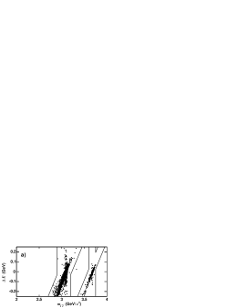
Figure 4: Charmonium veto regions (a) in the $B^{+}\rightarrow K^{+}e^{+}e^{-}$ channel. The points are simulated $J/\psi$ and $\psi{(2S)}$ events, with abundance equal to the mean number expected in 208 $\mbox{\,fb}^{-1}$. The projections onto (b) $m_{\ell^{+}\ell^{-}}$ and (c) $\Delta E$ are shown at right, indicating the high density of points at $(m_{\ell^{+}\ell^{-}},\Delta E)=(m_{\psi},0.0)$. The vertical band corresponds to events where the ${J\mskip-3.0mu/\mskip-2.0mu\psi\mskip 2.0mu}$ ($\psi{(2S)}$) and $K^{+}$ come from different $B$ decays. For $\Delta E<0$ it also includes events with mis-reconstructed $B\rightarrow J/\psi K^{*}$, $B\rightarrow\psi{(2S)}K^{*}$, and non-resonant charmonium decays. The slanted band corresponds to events with mis-measured lepton track momentum.

Backgrounds that peak in the $m_{ES}$ and $\Delta E$ variables in the same manner as the signal are either vetoed, or their rate is estimated from simulated data or control samples. The largest sources of peaking backgrounds are $B$ decays to charmonium: $B\rightarrow J/\psi K^{(*)}$ and $B\rightarrow\psi(2S)K^{(*)}$, where the $J/\psi$ or $\psi(2S)$ decays to a $\ell^{+}\ell^{-}$ pair. We therefore remove events in which the dilepton invariant mass is consistent with a $J/\psi$ or $\psi(2S)$, either with or without bremsstrahlung recovery in the electron channels. In cases where the lepton momentum is mis-measured, or the bremsstrahlung recovery algorithm fails to find a radiated photon, the dilepton mass will be shifted from the charmonium mass. In addition, the measured $\Delta E$ will be shifted away from zero in a correlated manner. We account for this by constructing a two-dimensional veto region in the $m_{\ell^{+}\ell^{-}}$ vs. $\Delta E$ plane as shown in Figure 4; the simulated points plotted demonstrate the expected background rejection. Within the veto region in data we find approximately 13700 $J/\psi$ events and 1000 $\psi(2S)$ events summed over all decay modes. These provide a high-statistics control sample useful for evaluating systematic uncertainties and selection efficiencies. The residual charmonium background after applying the veto is estimated from simulation to be between 0.0 and 1.6 events per decay mode.

Due to the 2-3% probability for misidentifying pions as muons, the $B\rightarrow K^{(*)}\mu^{+}\mu^{-}$ channels also receive a significant peaking background contribution from hadronic $B$ decays. The largest of these are $B^{-}\rightarrow D^{0}\pi^{-}$ where $D^{0}\rightarrow K^{-}\pi^{+}$ or $D^{0}\rightarrow K^{*-}\pi^{+}$, and $\overline{B^{0}}\rightarrow D^{+}\pi^{-}$ where $D^{+}\rightarrow\overline{K^{*0}}\pi^{+}$. These are suppressed by removing events in which the $K^{(*)}\mu$ invariant mass lies in the range $1.84<m_{K^{(*)}\mu}<1.90$ ${\mathrm{\,Ge\kern-1.00006ptV\!/}c^{2}}$. The remaining hadronic backgrounds come from charmless decays such as $B\rightarrow K^{(*)}\pi^{+}\pi^{-}$, $B\rightarrow K^{(*)}K^{+}\pi^{-}$, and $B\rightarrow K^{(*)}K^{+}K^{-}$. We measure the peaking background from these processes using data control samples of $B\rightarrow K^{(*)}h\mu$ events. These samples are selected with the same requirements as signal events, except hadron identification is required for the hadron candidate $h$ in place of muon identification. This yields samples of predominantly hadronic $B$ decays. We then weight each event by the muon misidentification rate for the hadron divided by its hadron identification efficiency. The hadronic peaking background is then extracted by a fit to the $m_{ES}$ distribution of these weighted events. This results in a total hadronic peaking background measurement of 0.4 - 2.3 events per muon decay channel. These backgrounds are suppressed by a factor of approximately 400 in the $B\rightarrow K^{(*)}e^{+}e^{-}$ channels due to the much lower probability of misidentifying pions as electrons.

There is an additional contribution to the peaking backgrounds in the electron channels from rare two-body decays. These include $B\rightarrow K^{*}\gamma$ with the $\gamma$ converting to an $e^{+}e^{-}$ pair in the detector, and $B\rightarrow K^{(*)}\pi^{0}$ or $B\rightarrow K^{(*)}\eta$, where the $\pi^{0}$ or $\eta$ undergoes a Dalitz decay to $e^{+}e^{-}\gamma$. These backgrounds are estimated from simulation to contribute 0.0 - 1.4 events per electron decay channel.

Table 1: Mean expected peaking backgrounds in 208$\mbox{\,fb}^{-1}$, for the individual $K^{(*)}\ell^{+}\ell^{-}$ decay modes after applying all selection requirements.

	All $q^{2}$	$0.1<q^{2}<8.41$	$q^{2}>10.24$
Mode		($\mathrm{\,Ge\kern-1.00006ptV}^{2}/c^{4}$)	($\mathrm{\,Ge\kern-1.00006ptV}^{2}/c^{4}$)
$K^{+}e^{+}e^{-}$	$0.7\pm 0.2$	$0.6\pm 0.2$	$0.1\pm 0.1$
$K^{+}\mu^{+}\mu^{-}$	$2.3\pm 0.5$	$1.4\pm 0.4$	$0.9\pm 0.1$
$K^{0}_{\scriptscriptstyle S}e^{+}e^{-}$	$0.01\pm 0.01$	$0.01\pm 0.01$	$0.0$
$K^{0}_{\scriptscriptstyle S}\mu^{+}\mu^{-}$	$0.4\pm 0.1$	$0.3\pm 0.1$	$0.1\pm 0.04$
$K^{*0}e^{+}e^{-}$	$3.0\pm 0.6$	$1.0\pm 0.5$	$0.6\pm 0.2$
$K^{*0}\mu^{+}\mu^{-}$	$1.4\pm 0.8$	$0.5\pm 0.3$	$0.2\pm 0.1$
$K^{*+}e^{+}e^{-}$	$0.9\pm 0.2$	$0.2\pm 0.2$	$0.2\pm 0.1$
$K^{*+}\mu^{+}\mu^{-}$	$0.6\pm 0.3$	$0.2\pm 0.1$	$0.2\pm 0.1$

The sum of peaking backgrounds from all sources is summarized in Table 1. As a function of $q^{2}$, all of the backgrounds from $K^{*}\gamma$ and $K^{(*)}\pi^{0}$ are localized in the region $0.0<q^{2}<0.1\mathrm{\,Ge\kern-1.00006ptV}^{2}/c^{4}$. Backgrounds from $J/\psi$ and $K^{(*)}\eta$ populate the region $0.1<q^{2}<8.41$ $\mathrm{\,Ge\kern-1.00006ptV}^{2}/c^{4}$, while the $\psi(2S)$ backgrounds contribute only to the region $q^{2}>10.24\mathrm{\,Ge\kern-1.00006ptV}^{2}/c^{4}$. The hadronic backgrounds occupy both the $0.1<q^{2}<8.41$ $\mathrm{\,Ge\kern-1.00006ptV}^{2}/c^{4}$ and $q^{2}>10.24\mathrm{\,Ge\kern-1.00006ptV}^{2}/c^{4}$ regions.

V Yield extraction procedure

We extract the signal yield and angular distributions using a multidimensional unbinned maximum likelihood fit. For $B\rightarrow K\ell^{+}\ell^{-}$, the total branching fraction is obtained from a two-dimensional fit to $m_{ES}$ and $\Delta E$. In the $B\rightarrow K^{*}\ell^{+}\ell^{-}$ modes, we add the reconstructed $K^{*}$ mass as a third fit variable. The signal shapes are parameterized in both $m_{ES}$ and $\Delta E$ by a Gaussian function plus a radiative tail described by an exponential power function. This takes the form

$$f(x)\propto\left\{\begin{array}[]{lrr}\exp(-\frac{(x-\overline{x})^{2}}{2\sigma^{2}})&;&(x-\overline{x})/\sigma>\alpha\\ A\times(B-\frac{x-\overline{x}}{\sigma})^{-n}&;&(x-\overline{x})/\sigma\leq\alpha\\ \end{array}\right.,$$

where $A\equiv(\frac{n}{|\alpha|})^{n}\times\exp(-|\alpha|^{2}/2)$ and $B\equiv\frac{n}{|\alpha|}-|\alpha|$. The variables $\overline{x}$ and $\sigma$ are the Gaussian peak and width, and $\alpha$ and $n$ are the point at which the function transitions to the power function and the exponent of the power function, respectively. The $m_{\rm ES}$ shape parameters $\overline{x}$, $\sigma$, $\alpha$, and $n$ are assumed to have a $\Delta E$ dependence of the form $c_{0}+c_{2}(\Delta E)^{2}$, determined empirically from simulation. The mean and width are fixed to the values derived by fitting the control sample of vetoed charmonium events. All other signal shape parameters are fixed to the values obtained from fits to simulated signal events. In the $B\rightarrow K^{*}\ell^{+}\ell^{-}$ mode, the mass of the $K^{*}$ is parameterized with a relativistic Breit-Wigner line shape.

The background is modeled as a sum of terms describing (1) combinatorial background; (2) peaking background; (3) cross-feed backgrounds; and, (4) in the $B\rightarrow K^{*}\ell^{+}\ell^{-}$ modes, backgrounds that peak in $m_{K\pi}$ at the $K^{*}$ mass but not in $m_{ES}$ and $\Delta E$. The combinatorial background is described by a product of an empirically derived threshold function in $m_{ES}$, a linear term in $\Delta E$, and the product of $\sqrt{m_{K\pi}-m_{K}-m_{\pi}}$ and a quadratic function of $m_{K\pi}$ for the $K^{*}$ modes. The form of the threshold function used to describe the background in $m_{ES}$ is $f(x)\propto x\sqrt{1-x^{2}}\exp{[-\zeta(1-x^{2})]}$, where $\zeta$ is a fit parameter and $x=m_{\rm ES}/E_{\rm b}^{*}$. The peaking background component has the same shape as the signal, with normalization fixed to the estimates of the mean peaking backgrounds (Table 1). The cross-feed component has a floating normalization to describe (a) background in $B\rightarrow K\ell^{+}\ell^{-}$ ($B\rightarrow K^{*}\ell^{+}\ell^{-}$) from $B\rightarrow K^{*}\ell^{+}\ell^{-}$ ($B\rightarrow K^{*}\pi\ell^{+}\ell^{-}$) events with a lost pion, and (b) background in $B\rightarrow K^{*}\ell^{+}\ell^{-}$ from $B\rightarrow K\ell^{+}\ell^{-}$ events with a randomly added pion. The backgrounds that peak only in $m_{K\pi}$ are described by the signal shape in $m_{K\pi}$ and the combinatorial background shape in $m_{ES}$ and $\Delta E$. The yield of this term is fixed to $(5\pm 5)\%$ of the total combinatorial background, as determined from simulation. As the shape parameters for term (1) and the normalizations for terms (1) and (3) are all free parameters of the fit, much of the background uncertainty propagates into the statistical uncertainty in the signal yield obtained from the fit.

The $C\!P$ asymmetry is also extracted from the fit in the $B^{+}\rightarrow K^{+}\ell^{+}\ell^{-}$ and $B\rightarrow K^{*}\ell^{+}\ell^{-}$ channels, where the flavor of the $b$ quark can be inferred from the charge of the final state $K^{(*)}$ hadron. As this cannot be done in the case of $B^{0}\rightarrow K^{0}_{\scriptscriptstyle S}\ell^{+}\ell^{-}$, we do not measure the $C\!P$ asymmetry in that mode. The possibility of a non-zero $C\!P$ asymmetry in the combinatorial background is accounted for by allowing its value to float in the fit. The $C\!P$ asymmetry of the peaking background is fixed to the value expected from the relative composition of background sources.

The partial branching fractions are measured by repeating the fit with the sample partitioned into $q^{2}$ bins. The signal efficiencies and peaking backgrounds are recomputed for each region of $q^{2}$. To determine the forward-backward asymmetry and $K^{*}$ polarization in bins of $q^{2}$, we also utilize fits to the $\cos\theta^{*}$ and $\cos\theta_{K}$ angular distributions. We follow the treatment of Ref. bib:krugerf0 to parameterize the angular distributions for signal. The signal shape in $\cos\theta_{K}$ is described by an underlying differential distribution which depends on the fraction of longitudinal polarization $F_{L}$ as

$$\frac{1}{\Gamma}\frac{d\Gamma}{d\cos\theta_{K}}=\frac{3}{2}F_{L}\cos^{2}\theta_{K}+\frac{3}{4}(1-F_{L})(1-\cos^{2}\theta_{K}).$$

The underlying differential rate for signal in $\cos\theta^{*}$ is then described in terms of $F_{L}$ and the forward-backward asymmetry term $A_{FB}$ which enters linearly in $\cos\theta^{*}$:

$$\frac{1}{\Gamma}\frac{d\Gamma}{d\cos\theta^{*}}=\frac{3}{4}F_{L}(1-\cos^{2}\theta^{*})+\frac{3}{8}(1-F_{L})(1+\cos^{2}\theta^{*})+$$

$$A_{FB}\cos\theta^{*}.$$

In the $B^{+}\rightarrow K^{+}\ell^{+}\ell^{-}$ mode, the most general distribution for $\cos\theta^{*}$ with non-zero $A_{FB}$ is given by:

$$\frac{1}{\Gamma}\frac{d\Gamma}{d\cos\theta^{*}}=\frac{3}{4}(1-F_{S})(1-\cos^{2}\theta^{*})+\frac{1}{2}F_{S}+A_{FB}\cos\theta^{*},$$

where $F_{S}$ is the relative contribution from scalar and pseudoscalar penguin amplitudes, and $A_{FB}$ arises from the interference of vector and scalar amplitudes bib:bobeth01 . In the Standard Model, both $F_{S}$ and $A_{FB}$ are expected to be negligibly small; their measurement is therefore a null test sensitive to new physics from scalar or pseudoscalar penguin processes.

The true angular distributions are altered by detector acceptance and efficiency effects. We account for this by multiplying the underlying distributions with efficiency functions $\epsilon(\cos\theta^{*})$ and $\epsilon(\cos\theta_{K})$ described by a non-parametric histogram PDF obtained from signal simulations.

The combinatorial background shapes in $\cos\theta^{*}$ and $\cos\theta_{K}$ are described by a histogram PDF drawn from control samples in the $m_{ES}$ and $\Delta E$ sidebands. The angular distribution of the peaking backgrounds are fixed in the fit. Additional components describing the angular distribution of cross-feed events and of mis-reconstructed signal events are included as histogram PDFs derived from simulated samples.

In the $B\rightarrow K^{*}\ell^{+}\ell^{-}$ modes we first perform a four-dimensional fit to $m_{ES}$, $\Delta E$, $m_{K\pi}$, and $\cos\theta_{K}$ to obtain $F_{L}$. Due to limited statistical sensitivity of $F_{L}$ to the $\cos\theta^{*}$ distribution, $F_{L}$ is fixed to the value measured from the $\cos\theta_{K}$ distribution in order to measure $A_{FB}$ from a fit to $m_{ES}$, $\Delta E$, $m_{K\pi}$, and $\cos\theta^{*}$. In the $B^{+}\rightarrow K^{+}\ell^{+}\ell^{-}$ modes, $A_{FB}$ and $F_{S}$ are simultaneously extracted directly from a three-dimensional fit to $m_{ES}$, $\Delta E$, and $\cos\theta^{*}$.

VI Systematic uncertainties

VI.1 Branching fractions

In evaluating systematic uncertainties in the branching fractions, we consider both errors that affect the signal efficiency estimate, and errors arising from the maximum likelihood fit. Sources of uncertainties that affect the efficiency are: charged-particle tracking (0.8% per lepton, 1.4% per charged hadron), charged-particle identification (0.5% per electron pair, 1.3% per muon pair, 0.2% per pion, 0.6% per kaon), the continuum background suppression selection (0.3%–2.2% depending on the mode), the $B\kern 1.79993pt\overline{\kern-1.79993ptB}{}$ background suppression selection (0.6%–2.1%), $K_{\scriptscriptstyle S}^{0}$ selection (0.9%), and signal simulation statistics (0.4%–0.7%). The estimated number of $B\kern 1.79993pt\overline{\kern-1.79993ptB}{}$ events in our data sample has an uncertainty of 1.1%. We use the high-statistics sample of events that fail the charmonium veto to bound the systematic uncertainties associated with the continuum suppression Fisher discriminant, the $B\kern 1.79993pt\overline{\kern-1.79993ptB}{}$ likelihood suppression selection, and charged particle identification. The Fisher discriminant and $B\kern 1.79993pt\overline{\kern-1.79993ptB}{}$ likelihood ratio for $B^{+}\rightarrow K^{+}e^{+}e^{-}$ are illustrated in Figure 5 for data and simulation in the $J/\psi$ control sample. An additional systematic uncertainty in the efficiency results from the choice of form factor model, which alters the $q^{2}$ distribution of the signal. We take this uncertainty to be the maximum efficiency variation obtained from a set of recent models bib:TheoryD ; bib:TheoryE ; bib:TheoryBa ; bib:ErratumTheoryBa ; bib:TheoryBc ; the uncertainty is computed separately for each mode and varies in size from 1.1% to 8.3%.

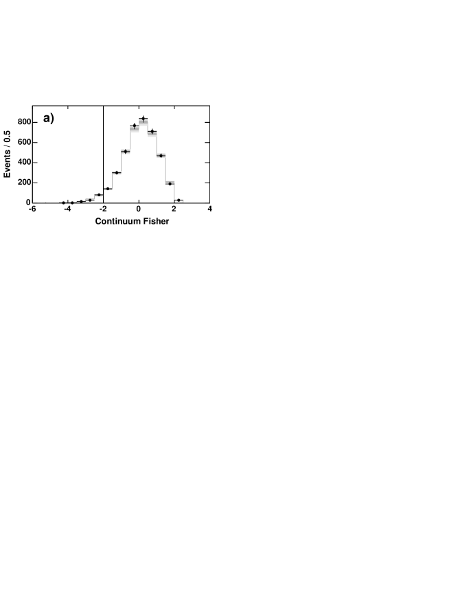
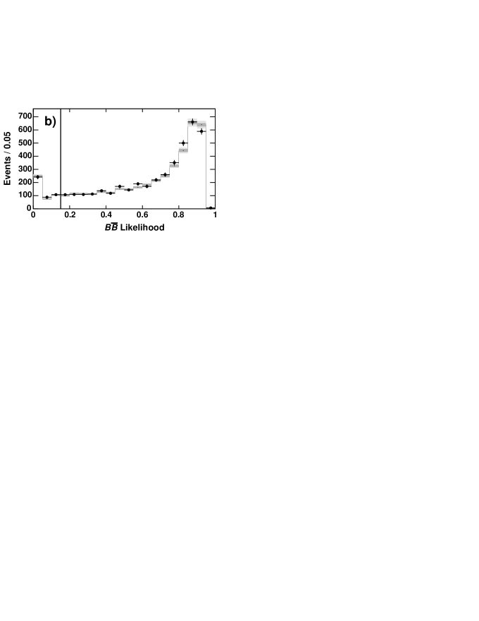
Figure 5: Distribution of (a) the Fisher discriminant and (b) the $B\kern 1.79993pt\overline{\kern-1.79993ptB}{}$ likelihood ratio for $B^{+}\rightarrow K^{+}e^{+}e^{-}$ events in the $J/\psi$ veto sample. The points are data; the gray bands are simulated events, with a simulation uncertainty given by the band height. The dark gray portion represents the uncertainty due to simulation statistics, while the additional uncertainty due to the $B\rightarrow J/\psi K^{+}$ branching fraction is represented by the light gray band height. Events to the right of the vertical line are selected.

Systematic uncertainties on the signal yields obtained from the maximum-likelihood fit arise from three sources: uncertainties in the parameters describing the signal shapes, uncertainties in the combinatorial background shape, and uncertainties in the peaking backgrounds. The uncertainties in the means and widths of the signal shapes are obtained by comparing data and simulated data in $B\rightarrow{J\mskip-3.0mu/\mskip-2.0mu\psi\mskip 2.0mu}K^{(*)}$ control samples. For modes with electrons, we also vary the fraction of signal events in the tail of the $\Delta E$ distribution by varying the exponent $n$ in the exponential power function. Signal shape uncertainties are typically 2–4% of the signal yield. To evaluate the uncertainty due to the background shape, we reevaluate the fit yields with three different parameterizations: (1) an exponential shape for $\Delta E$, (2) a quadratic shape for $\Delta E$, and (3) an $m_{ES}$ background shape parameter $\zeta$ which is linearly correlated with $\Delta E$. In modes with a $K^{*}$, we also vary the yield of the background component which peaks in $m_{K\pi}$ but not in $m_{ES}$ or $\Delta E$ by 100% of itself. The induced uncertainty in the signal yield due to the background shape is 4–6% for $B\rightarrow K\ell^{+}\ell^{-}$ modes and increases to 8–12% for $B\rightarrow K^{*}\ell^{+}\ell^{-}$ modes, where the backgrounds are generally larger. Uncertainties in the peaking background induce an uncertainty in the signal yields of 2–5%; this is obtained by varying the expected peaking background yield within its $\pm 1\sigma$ uncertainties. The total systematic uncertainty in the fitted signal yield induces a systematic uncertainty $\Delta{\cal B}_{\textrm{fit}}$ in the measured branching fraction; this uncertainty is shown for each of the branching fraction fits in Tables 2 and  3.

VI.2 $C\!P$ asymmetry

The systematic uncertainties in the measurement of $A_{C\!P}$ include errors due both to detector efficiency effects and to the asymmetry in the peaking background component. The error associated with the detector efficiency is obtained by comparing the value of $A_{C\!P}$ measured in the charmonium control samples with the expected value of zero; agreement with zero is obtained with a precision of 1.2% for $B^{+}\rightarrow K^{+}\ell^{+}\ell^{-}$ and 2.1% for $B\rightarrow K^{*}\ell^{+}\ell^{-}$. The uncertainty due to the peaking background is evaluated by varying the expected $C\!P$ asymmetry of the peaking backgrounds within their uncertainties. The possible $C\!P$ asymmetry in the charmonium and $B\rightarrow K^{*}\gamma$ peaking backgrounds is highly constrained from previous measurements; any asymmetry in the Dalitz decays is suppressed by their relatively small contribution to the peaking background. In contrast, the hadronic peaking background in the muon modes could exhibit a significant $C\!P$ asymmetry; this is measured directly from the asymmetry of the hadronic control sample described in Section IV.2 with an uncertainty dominated by the statistics of the sample. This induces an uncertainty in the measured $A_{C\!P}$ of 1% for $B^{+}\rightarrow K^{+}\ell^{+}\ell^{-}$ and 2% for $B\rightarrow K^{*}\ell^{+}\ell^{-}$. Other systematic uncertainties induced by the fitting procedure, as computed above for the branching fraction measurements, are found to be negligible.

VI.3 Angular distributions

Systematic uncertainties related to the angular distributions of the efficiency are estimated by comparing the values of $A_{FB}$, $F_{S}$, and $F_{L}$ measured in the relevant charmonium control samples with their expected values. For $B\rightarrow{J\mskip-3.0mu/\mskip-2.0mu\psi\mskip 2.0mu}K$ and $B\rightarrow{J\mskip-3.0mu/\mskip-2.0mu\psi\mskip 2.0mu}K^{*}$ we measure an $A_{FB}$ consistent with zero and with a precision of 0.01 and 0.02, respectively. For $B\rightarrow{J\mskip-3.0mu/\mskip-2.0mu\psi\mskip 2.0mu}K^{*}$, we measure $F_{L}$ to be consistent with the previous BABAR measurement bib:cos2beta , with a precision of 0.05. For $B\rightarrow{J\mskip-3.0mu/\mskip-2.0mu\psi\mskip 2.0mu}K$ we measure $F_{S}$ consistent with zero and with a precision of 0.03.

Further systematic uncertainties are evaluated by repeating the fit with alternative shapes assumed for the background components: (1) the shape of mis-reconstructed signal events is fixed instead to the shape of correctly reconstructed signal, (2) the combinatorial background shape is drawn from alternative ranges of $m_{ES}$ and $\Delta E$, and from the sample of events that fail the $B\kern 1.79993pt\overline{\kern-1.79993ptB}{}$ likelihood selection, and (3) the angular distributions of the peaking backgrounds are varied within their statistical uncertainties. Systematic uncertainties from backgrounds induce uncertainties in $F_{L}$ and $A_{FB}$ of 0.05–0.18, depending on the relative amount of background, and are the largest systematic uncertainty. $F_{S}$ is more sensitive to the background shape, with an induced systematic uncertainty of 0.45.

In the fit to $\cos\theta^{*}$ in the $B\rightarrow K^{*}\ell^{+}\ell^{-}$ decay modes, the value of $F_{L}$ is fixed to the result obtained from the fit to the $\cos\theta_{K}$ distribution. This introduces an additional parametric uncertainty of 0.01 on the measured value of $A_{FB}$ , which we evaluate by varying $F_{L}$ within the uncertainty of the measurement.

VII Results

VII.1 Branching fractions

We first perform the fit separately for each of the eight decay modes to extract the branching fractions integrated over all $q^{2}$. In the branching fraction fits, the efficiency is defined such that the total branching fraction includes the estimated signal that is lost due to the charmonium vetos. The results for the individual decay modes are shown in Table 2. We then perform a combined fit to the appropriate combinations of modes to extract the $B\rightarrow K\ell^{+}\ell^{-}$ and $B\rightarrow K^{*}\ell^{+}\ell^{-}$ branching fractions. We combine charged and neutral modes by constraining the total width ratio $\Gamma(B^{0})/\Gamma(B^{+})$ to the world average ratio of lifetimes $\tau(B^{+})/\tau(B^{0})=1.071\pm 0.009$ bib:pdglifetime . In the $B\rightarrow K^{*}\ell^{+}\ell^{-}$ mode, we add the additional constraint $\Gamma(B\rightarrow K^{*}\mu^{+}\mu^{-})/\Gamma(B\rightarrow K^{*}e^{+}e^{-})=0.75$ to account for the enhancement due to the pole at low $q^{2}$ in the electron channel bib:TheoryA . The final branching fractions are expressed in terms of the $B^{0}\rightarrow K^{(*)0}\mu^{+}\mu^{-}$ channels. With these constraints, we find the lepton-flavor averaged, $B$-charge averaged branching fractions

$${\cal B}(B\rightarrow K\ell^{+}\ell^{-})=(0.34\pm 0.07\pm 0.02)\times 10^{-6},$$

$${\cal B}(B\rightarrow K^{*}\ell^{+}\ell^{-})=(0.78^{+0.19}_{-0.17}\pm 0.11)\times 10^{-6},$$

where the first error is statistical and the second systematic. The projections of the data overlayed with the combined fit results are shown in Figures 6 and  7. The signal significance is computed as $\sqrt{2\Delta\ln(\cal{L})}$, where $\Delta\ln(\cal{L})$ is the difference between the likelihood of the best fit and that of the null signal hypothesis. Systematic uncertainties are incorporated in the significance estimate by simultaneously applying all variations that result in a lower signal yield before computing the change in likelihood. The significance of the signal including statistical and systematic uncertainties is $6.6$ standard deviations for the $B\rightarrow K\ell^{+}\ell^{-}$ mode and $5.7$ standard deviations for the $B\rightarrow K^{*}\ell^{+}\ell^{-}$ mode. The secondary peak in the $\Delta E$ sideband of $B\rightarrow K\ell^{+}\ell^{-}$ results from the fit component describing events with a lost pion, either from $B\rightarrow K^{*}\ell^{+}\ell^{-}$ or from events in which a $b\rightarrow s\ell^{+}\ell^{-}$ decay results in a $K\pi\ell^{+}\ell^{-}$ final state without proceeding through an intermediate $K^{*}$ resonance. The normalization and mean $\Delta E$ of this component are free parameters in the fit. Examination of these events shows that the addition of a charged or neutral pion results in a $B\rightarrow K^{*}\ell^{+}\ell^{-}$ or $B\rightarrow K\pi\ell^{+}\ell^{-}$ signal candidate. Using simulated signal decays, we find the effect of these events on the $B\rightarrow K\ell^{+}\ell^{-}$ signal yield is negligible.

We further perform a set of combined fits with the sample partitioned into final states containing muons and electrons, and into charged and neutral final states, modifying the constraints as appropriate. The results from all such fits are summarized in Table 3.

Table 2: Results from fits to the individual $K^{(*)}\ell^{+}\ell^{-}$ decay modes for all $q^{2}$. The columns from left are: decay mode, fitted signal yield, signal efficiency, relative uncertainty on the branching fraction due to the systematic error on the efficiency estimate, systematic error from the fit, and the resulting branching fraction (with statistical and systematic errors).

		$\epsilon$	$\Delta\cal B_{\rm eff}$	$\Delta\cal B_{\rm fit}$	$\cal B$
Mode	Yield	$(\%)$	$(\%)$	$(10^{-6})$	$(10^{-6})$
$K^{+}e^{+}e^{-}$	$25.9^{+7.4}_{-6.5}$	$26.6$	$\pm 3.7$	$\pm 0.02$	$0.42^{+0.12}_{-0.11}\pm 0.02$
$K^{+}\mu^{+}\mu^{-}$	$10.9^{+5.1}_{-4.3}$	$15.4$	$\pm 4.1$	$\pm 0.03$	$0.31^{+0.15}_{-0.12}\pm 0.03$
$K^{0}e^{+}e^{-}$	$2.4^{+2.8}_{-2.0}$	$22.8$	$\pm 9.6$	$\pm 0.01$	$0.13^{+0.16}_{-0.11}\pm 0.02$
$K^{0}\mu^{+}\mu^{-}$	$6.3^{+3.6}_{-2.8}$	$13.6$	$\pm 8.3$	$\pm 0.04$	$0.59^{+0.33}_{-0.26}\pm 0.07$
$K^{*0}e^{+}e^{-}$	$29.4^{+9.5}_{-8.4}$	$18.6$	$\pm 4.9$	$\pm 0.09$	$1.04^{+0.33}_{-0.29}\pm 0.11$
$K^{*0}\mu^{+}\mu^{-}$	$15.9^{+7.0}_{-5.9}$	$11.9$	$\pm 5.8$	$\pm 0.11$	$0.87^{+0.38}_{-0.33}\pm 0.12$
$K^{*+}e^{+}e^{-}$	$6.1^{+6.3}_{-5.3}$	$15.7$	$\pm 6.8$	$\pm 0.37$	$0.75^{+0.76}_{-0.65}\pm 0.38$
$K^{*+}\mu^{+}\mu^{-}$	$4.7^{+4.6}_{-3.4}$	$9.3$	$\pm 7.1$	$\pm 0.13$	$0.97^{+0.94}_{-0.69}\pm 0.14$

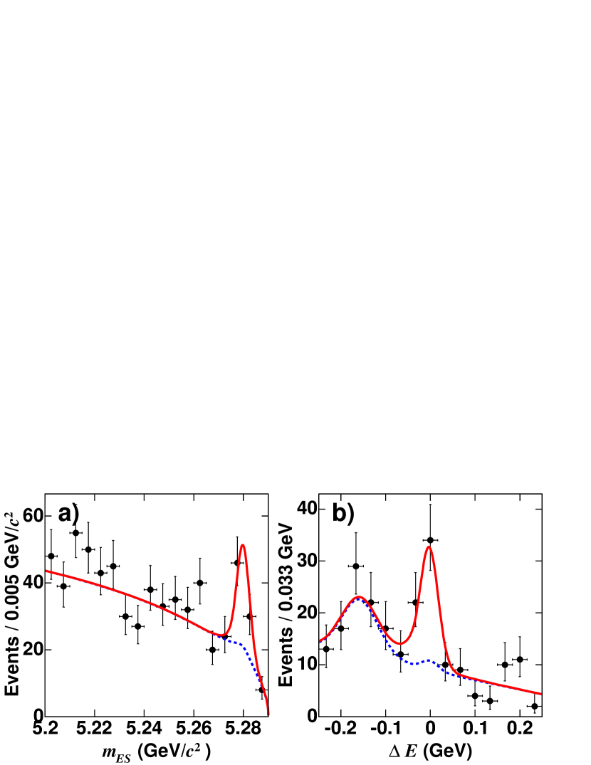
Figure 6: Distributions of the fit variables in $K\ell^{+}\ell^{-}$ data (points), compared with projections of the combined fit (curves): (a) $m_{\rm ES}$ distribution after requiring $-0.11<\Delta E<0.05\ {\rm GeV}$ and (b) $\Delta E$ distribution after requiring $|m_{\rm ES}-m_{B}|<6.6\ {\rm MeV}/c^{2}$. The solid curve is the sum of all fit components, including signal; the dashed curve is the sum of all background components.

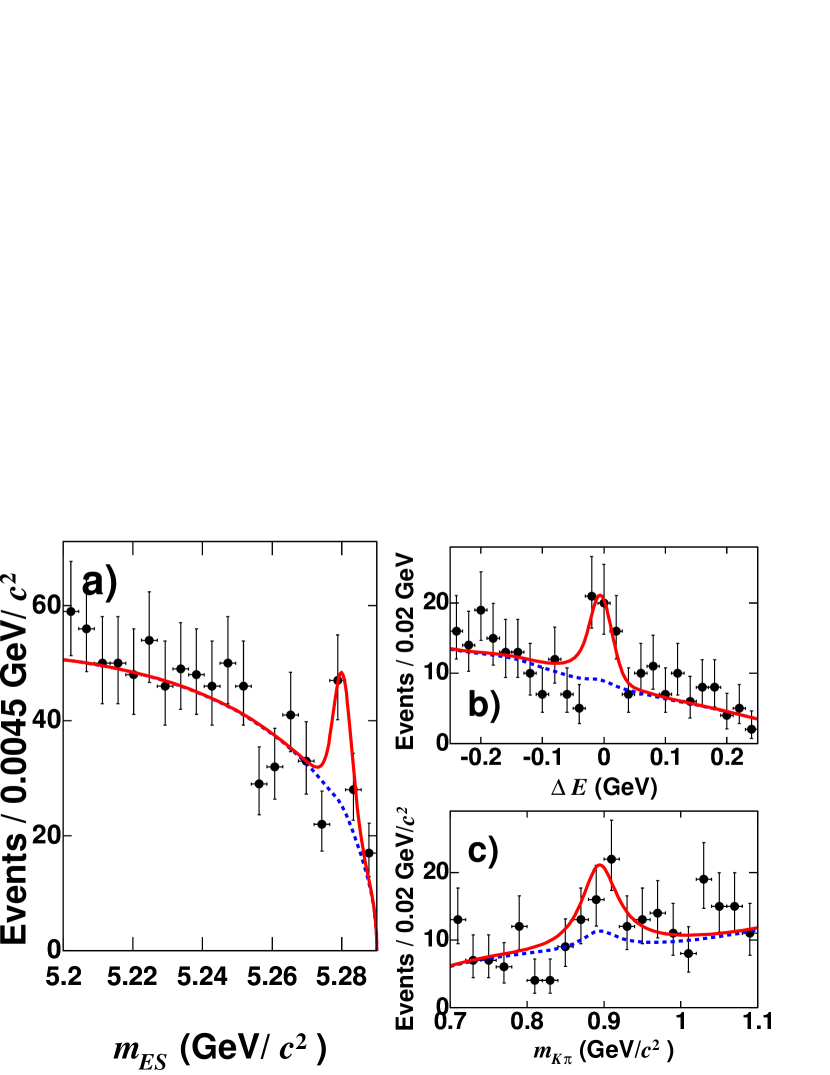
Figure 7: Distributions of the fit variables in $K^{*}\ell^{+}\ell^{-}$ data (points), compared with projections of the combined fit (curves): (a) $m_{ES}$ after requiring $-0.11<\Delta E<0.05\ {\rm GeV}$ and $0.817<m_{K\pi}<0.967\ {\rm GeV}/c^{2}$, (b) $\Delta E$ after requiring $|m_{\rm ES}-m_{B}|<6.6\ {\rm MeV}/c^{2}$, $0.817<m_{K\pi}<0.967\ {\rm GeV}/c^{2}$, and (c) $m_{K\pi}$ after requiring $|m_{\rm ES}-m_{B}|<6.6\ {\rm MeV}/c^{2}$ and $-0.11<\Delta E<0.05\ {\rm GeV}$. The solid curve is the sum of all fit components, including signal; the dashed curve is the sum of all background components.

Table 3: Results from fits to combined $K^{(*)}\ell^{+}\ell^{-}$ decay modes for all $q^{2}$. The columns from left are: decay mode combination, fitted signal yield, relative uncertainty on the branching fraction due to the systematic error on the efficiency estimate, systematic error on the branching fraction introduced by the systematic error on the fitted signal yield, and the resulting branching fraction (with statistical and systematic errors). The constraints for each combined fit are described in the text.

	Yield	$\Delta\cal B_{\rm eff}$	$\Delta\cal B_{\rm fit}$	$\cal B$
Mode	(events)	$(\%)$	$(10^{-6})$	$(10^{-6})$
$Ke^{+}e^{-}$	$28.1^{+7.8}_{-7.0}$	$\pm 4.7$	$\pm 0.02$	$0.33^{+0.09}_{-0.08}\pm 0.02$
$K\mu^{+}\mu^{-}$	$17.3^{+6.2}_{-5.4}$	$\pm 4.8$	$\pm 0.03$	$0.35^{+0.13}_{-0.11}\pm 0.03$
$K^{+}\ell^{+}\ell^{-}$	$36.7^{+8.8}_{-7.9}$	$\pm 3.7$	$\pm 0.02$	$0.38^{+0.09}_{-0.08}\pm 0.02$
$K^{0}\ell^{+}\ell^{-}$	$8.2^{+4.5}_{-3.6}$	$\pm 9.0$	$\pm 0.02$	$0.29^{+0.16}_{-0.13}\pm 0.03$
$K\ell^{+}\ell^{-}$	$45.5^{+9.8}_{-8.9}$	$\pm 4.6$	$\pm 0.02$	$0.34^{+0.07}_{-0.07}\pm 0.02$
$K^{*}e^{+}e^{-}$	$36.2^{+11.2}_{-10.0}$	$\pm 5.2$	$\pm 0.13$	$0.97^{+0.30}_{-0.27}\pm 0.14$
$K^{*}\mu^{+}\mu^{-}$	$20.7^{+8.1}_{-7.0}$	$\pm 5.9$	$\pm 0.11$	$0.88^{+0.35}_{-0.30}\pm 0.12$
$K^{*0}\ell^{+}\ell^{-}$	$45.3^{+11.6}_{-10.5}$	$\pm 5.0$	$\pm 0.08$	$0.81^{+0.21}_{-0.19}\pm 0.09$
$K^{*+}\ell^{+}\ell^{-}$	$11.5^{+8.0}_{-6.6}$	$\pm 6.6$	$\pm 0.20$	$0.73^{+0.50}_{-0.42}\pm 0.21$
$K^{*}\ell^{+}\ell^{-}$	$57.1^{+13.7}_{-12.5}$	$\pm 5.3$	$\pm 0.10$	$0.78^{+0.19}_{-0.17}\pm 0.11$
Pole excluded
$K^{*}e^{+}e^{-}$	$23.6^{+9.4}_{-8.3}$	$\pm 5.2$	$\pm 0.11$	$0.63^{+0.25}_{-0.22}\pm 0.11$
$K^{*}\mu^{+}\mu^{-}$	$20.7^{+8.1}_{-7.0}$	$\pm 5.9$	$\pm 0.11$	$0.88^{+0.34}_{-0.30}\pm 0.12$
$K^{*0}\ell^{+}\ell^{-}$	$34.8^{+10.4}_{-9.3}$	$\pm 5.0$	$\pm 0.10$	$0.75^{+0.22}_{-0.20}\pm 0.10$
$K^{*+}\ell^{+}\ell^{-}$	$9.5^{+7.0}_{-5.7}$	$\pm 6.6$	$\pm 0.19$	$0.73^{+0.53}_{-0.44}\pm 0.19$
$K^{*}\ell^{+}\ell^{-}$	$44.3^{+12.2}_{-11.1}$	$\pm 5.3$	$\pm 0.11$	$0.73^{+0.20}_{-0.18}\pm 0.11$

If the pole region is removed by requiring $q^{2}>0.1\mathrm{\,Ge\kern-1.00006ptV}^{2}/c^{4}$, the constrained ratio between $B\rightarrow K^{*}\mu^{+}\mu^{-}$ and $B\rightarrow K^{*}e^{+}e^{-}$ in the combined fit is modified from 0.75 to 1. Repeating the combined fit with this modification, we obtain

$${\cal B}(B\rightarrow K^{*}\ell^{+}\ell^{-})_{(q^{2}>0.1\mathrm{\,Ge\kern-0.70004ptV}^{2}/c^{4})}=(0.73^{+0.20}_{-0.18}\pm 0.11)\times 10^{-6}.$$

The results of the combined fits in the various subsamples with the pole region removed are shown in Table 3. We observe good agreement in the branching fraction obtained in all of the subsamples, both with and without the pole region included. The measured total rates are consistent with the range of Standard Model rates predicted in Ref. bib:TheoryA . The $B\rightarrow K\ell^{+}\ell^{-}$ rate is significantly lower than the range given by Ref. bib:TheoryC .

From the separate fits to the muon and electron channels integrated over all $q^{2}$, we obtain the ratios

$$R_{K}=1.06\pm 0.48\pm 0.08,$$

$$R_{K^{*}}=0.91\pm 0.45\pm 0.06,$$

consistent with the SM predictions of 1.00 and 0.75, respectively. If instead the pole region is excluded from the $B\rightarrow K^{*}\ell^{+}\ell^{-}$ channels, we find

$$R_{K^{*},(q^{2}>0.1\mathrm{\,Ge\kern-0.70004ptV}^{2}/c^{4})}=1.40\pm 0.78\pm 0.10,$$

where this ratio is expected to be 1 in the SM.

VII.2 $C\!P$ asymmetry

From the fit to the combined modes integrated over all $q^{2}$, we find the direct $C\!P$ asymmetries

$$A_{C\!P}(B^{+}\rightarrow K^{+}\ell^{+}\ell^{-})=-0.07\pm 0.22\pm 0.02,$$

$$A_{C\!P}(B\rightarrow K^{*}\ell^{+}\ell^{-})=+0.03\pm 0.23\pm 0.03,$$

where the first error is statistical and the second systematic. The measured values in both channels are consistent with the SM expectation of a negligible direct $C\!P$ asymmetry.

VII.3 Partial branching fractions

The partial branching fractions obtained from the fits to $m_{ES}$, $\Delta E$, and $m_{K\pi}$ in two bins of $q^{2}$ are shown in Table 4. The results are generally consistent with the $q^{2}$ dependence predicted in recent Standard Model based form factor calculations (Figure 8).

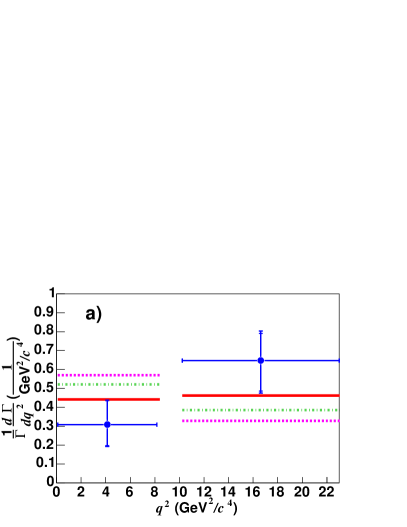
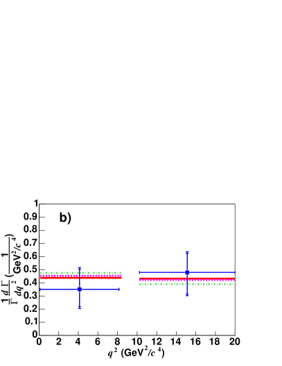
Figure 8: Partial branching fractions in bins of $q^{2}$ for (a) $B\rightarrow K\ell^{+}\ell^{-}$ and (b) $B\rightarrow K^{*}\ell^{+}\ell^{-}$, normalized to the total measured branching fraction. The points with error bars are data, the lines represent the central values of Standard Model predictions based on the form factor models of Refs. bib:TheoryD ; bib:TheoryE (solid lines),  bib:TheoryBc (dashed lines), and  bib:TheoryBa ; bib:ErratumTheoryBa (dot-dashed lines).

Table 4: Results from fits to the combined $K^{(*)}\ell^{+}\ell^{-}$ decay modes in bins of $q^{2}$. The columns from left to right are: fitted $q^{2}$ range, partial branching fraction, longitudinal $K^{*}$ polarization $F_{L}$, and the lepton forward-backward asymmetry $A_{FB}$. The first and second uncertainties are statistical and systematic, respectively. In $B\rightarrow K\ell^{+}\ell^{-}$, $A_{FB}$ is measured in the charged $B$ decay modes only. The constraints for each combined fit are described in the text. The partial branching fractions are defined such that they include the estimated rate within the vetoed $J/\psi$ and $\psi(2S)$ resonance regions where appropriate.

	$B\rightarrow K^{*}\ell^{+}\ell^{-}$
$q^{2}(\mathrm{\,Ge\kern-1.00006ptV}^{2}/c^{4})$	$\cal B$($10^{-6}$)	$F_{L}$	$A_{FB}$
$0.1-8.41$	$0.27^{+0.12}_{-0.10}\pm 0.05$	$0.77^{+0.63}_{-0.30}\pm 0.07$	$>0.19$ (95%CL)
$>10.24$	$0.37^{+0.13}_{-0.11}\pm 0.05$	$0.51^{+0.22}_{-0.25}\pm 0.08$	$0.72^{+0.28}_{-0.26}\pm 0.08$
$>0.1$	$0.73^{+0.20}_{-0.18}\pm 0.11$	$0.63^{+0.18}_{-0.19}\pm 0.05$	$>0.55$ (95%CL)
	$B\rightarrow K\ell^{+}\ell^{-}$
$q^{2}(\mathrm{\,Ge\kern-1.00006ptV}^{2}/c^{4})$	$\cal B$($10^{-6}$)	$F_{S}$	$A_{FB}$
$0.1-8.41$	$0.10^{+0.04}_{-0.04}\pm 0.01$	0	$-0.49^{+0.51}_{-0.99}\pm 0.18$
$>10.24$	$0.22^{+0.05}_{-0.05}\pm 0.02$	0	$0.26^{+0.23}_{-0.24}\pm 0.03$
$>0.1$	$0.34^{+0.07}_{-0.07}\pm 0.02$	$0.81^{+0.58}_{-0.61}\pm 0.46$	$0.15^{+0.21}_{-0.23}\pm 0.08$

VII.4 $K^{*}$ polarization

The fit projections for the $\cos\theta_{K}$ distribution in bins of $q^{2}$ are shown in Figure 12 of Appendix A. The resulting values for the fraction of longitudinal polarization $F_{L}$ are listed in Table 4. Combining all events with $q^{2}>0.1\mathrm{\,Ge\kern-1.00006ptV}^{2}/c^{4}$, we find

$${F_{L}}{(B\rightarrow K^{*}\ell^{+}\ell^{-})}_{(q^{2}>0.1\mathrm{\,Ge\kern-0.70004ptV}^{2}/c^{4})}=0.63^{+0.18}_{-0.19}\pm 0.05,$$

where the first error is statistical, and the second systematic.

The measured values of $F_{L}$ are consistent with the SM expectation in both $q^{2}$ ranges (Figure 9) and integrated over all $q^{2}>0.1\mathrm{\,Ge\kern-1.00006ptV}^{2}/c^{4}$. However, the large statistical uncertainties do not allow the determination of the sign of $C_{7}$ from this measurement at present.

VII.5 Lepton forward-backward asymmetry

The fit projections for the $\cos\theta^{*}$ distribution in the $B^{+}\rightarrow K^{+}\ell^{+}\ell^{-}$ mode are shown in Figure 13 of Appendix A. Combining all events with $q^{2}>0.1\mathrm{\,Ge\kern-1.00006ptV}^{2}/c^{4}$, we find for the $B^{+}\rightarrow K^{+}\ell^{+}\ell^{-}$ mode

$${A_{FB}}{(B^{+}\rightarrow K^{+}\ell^{+}\ell^{-})}_{(q^{2}>0.1\mathrm{\,Ge\kern-0.70004ptV}^{2}/c^{4})}=0.15^{+0.21}_{-0.23}\pm 0.08,$$

$${F_{S}}{(B^{+}\rightarrow K^{+}\ell^{+}\ell^{-})}_{(q^{2}>0.1\mathrm{\,Ge\kern-0.70004ptV}^{2}/c^{4})}=0.81^{+0.58}_{-0.61}\pm 0.46,$$

where the first errors are statistical, and the second systematic. The correlation coefficient between these two meaurements is +0.23. Both $A_{FB}$ and $F_{S}$ are consistent with the SM prediction of zero. As a cross-check, we have also performed similar fits in the low and high $q^{2}$ regions for $A_{FB}$, where due to limited statistics $F_{S}$ must be fixed to zero; the resulting asymmetries are $-0.49^{+0.51}_{-0.99}\pm 0.18$ and $0.26^{+0.23}_{-0.24}\pm 0.03$, respectively, which again are both consistent with zero asymmetry.

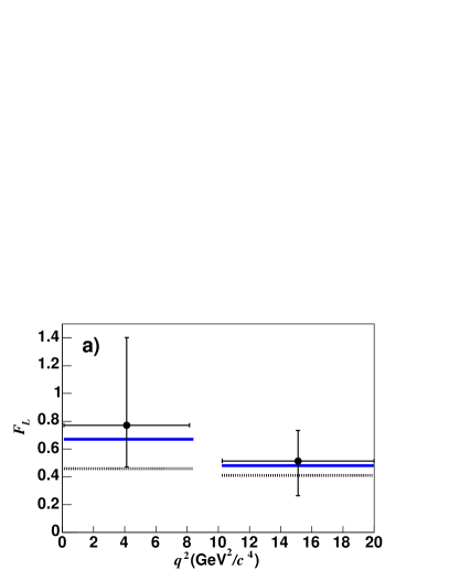
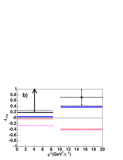
Figure 9: (a) $F_{L}(q^{2})$ and (b) $A_{FB}(q^{2})$ in $B\rightarrow K^{*}\ell^{+}\ell^{-}$. The points with error bars are data, with the arrow at low $q^{2}$ in $A_{FB}$ indicating the $95\%$ CL allowed region. The lines represent the predictions of the SM (solid lines), $C_{7}^{\rm eff}=-C_{7}(SM)$ (dotted lines), $C_{9}^{\rm eff}C_{10}^{\rm eff}=-C_{9}C_{10}(SM)$ (dashed lines), and $C_{7}^{\rm eff},C_{9}^{\rm eff}C_{10}^{\rm eff}=-C_{7}(SM),-C_{9}C_{10}(SM)$ (dot-dashed lines) with the form factor model of Ref. bib:TheoryE . In the case of $F_{L}$, the two solutions with $C_{9}^{\rm eff}C_{10}^{\rm eff}=-C_{9}C_{10}(SM)$ are not displayed; they are nearly identical to the two shown.

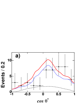
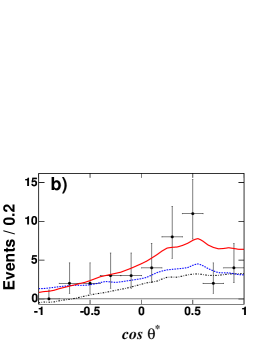
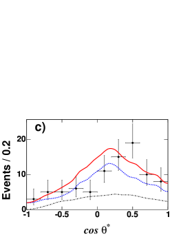
Figure 14: Distributions of the fit variable $\cos\theta^{*}$ in $B\rightarrow K^{*}\ell^{+}\ell^{-}$ data (points), compared with projections of the combined fit (curves) after requiring $-0.11<\Delta E<0.05\ {\rm GeV}$, $|m_{\rm ES}-m_{B}|<6.6\ {\rm MeV}/c^{2}$, and $0.817<m_{K\pi}<0.967\ {\rm GeV}/c^{2}$. The solid curve is the sum of all fit components, the dashed curve is the sum of all background components, and the dot-dashed curve is the signal component. The $q^{2}$ regions (a) $0.1<q^{2}<8.41\mathrm{\,Ge\kern-1.00006ptV}^{2}/c^{4}$, (b) $q^{2}>10.24\mathrm{\,Ge\kern-1.00006ptV}^{2}/c^{4}$, and (c) $q^{2}>0.1\mathrm{\,Ge\kern-1.00006ptV}^{2}/c^{4}$ are shown. The combined fits shown for (a) and (c) are performed by fixing $A_{FB}$ to its maximal physical value.

The fit projections for the $\cos\theta^{*}$ distribution in the $B\rightarrow K^{*}\ell^{+}\ell^{-}$ mode are shown in Figure 14 of Appendix A, and the resulting values of $A_{FB}$ listed in Table 4. We find a large positive asymmetry in the high $q^{2}$ region, consistent with the SM expectation. This disfavors new physics scenarios in which the product of the $C^{\rm eff}_{9}$ and $C^{\rm eff}_{10}$ Wilson coefficients have the same magnitude but opposite relative sign as in the SM, which would result in a large negative asymmetry at high $q^{2}$ (Figure 9).

For the low $q^{2}$ region and the region integrated over all $q^{2}>0.1\mathrm{\,Ge\kern-1.00006ptV}^{2}/c^{4}$, the $A_{FB}$ value corresponding to the maximum likelihood is positive, but is near the boundary at which a larger $A_{FB}$ will result in a negative, undefined value for the extended likelihood function. For these maximally asymmetric cases the $A_{FB}$ result is computed as a one-sided lower limit using a toy Monte Carlo method. For fixed values of $A_{FB}$, we randomly generate from the experimentally measured PDFs an ensemble of toy experiments, and find the value of $A_{FB}$ for which $5\%$ of experiments in the ensemble have a maximium likelihood fit resulting in a maximally positive $A_{FB}$. The uncertainties in the other PDF parameters are accounted for by varying them randomly for each generated experiment in the ensemble according to normal distributions determined by the parameters’ measured central values and uncertainties. We account for systematic uncertainties that do not correspond to continuous PDF parameters, such as the choice of combinatorial background PDFs for $\cos\theta^{*}$, by generating ensembles for each PDF variation and choosing that which results in the lowest lower limit. With this method, we find $A_{FB}>0.19$ at 95% CL for the low $q^{2}$ region. Combining all events with $q^{2}>0.1\mathrm{\,Ge\kern-1.00006ptV}^{2}/c^{4}$, we find for the $B\rightarrow K^{*}\ell^{+}\ell^{-}$ mode at $95\%$ CL

$${A_{FB}}{(B\rightarrow K^{*}\ell^{+}\ell^{-})}_{(q^{2}>0.1\mathrm{\,Ge\kern-0.70004ptV}^{2}/c^{4})}>0.55.$$

The corresponding fit projections shown in Figure 14 are produced by fixing the $A_{FB}$ of the signal component to its maximum physical value.

VII.6 Search for lepton flavor-violation

We extract the signal yield in the $B\rightarrow Ke\mu$ and $B\rightarrow K^{*}e\mu$ final states in a similar manner as the $K^{(*)}\ell^{+}\ell^{-}$ decays, with the particle identification requirements modified to select $e^{\pm}\mu^{\mp}$ pairs. The signal efficiencies for these modes are determined from simulations where the $B$ decays according to a simple three-particle phase space model. The results are shown in Table 5. As any physics that allows these decays will not necessarily affect the $e^{+}\mu^{-}$ and $e^{-}\mu^{+}$ states equally, we quote results for each charge state in addition to combined charge-averaged results. The projections of the data overlayed with the results of the combined fits are shown in Figures 10 and  11. We find no evidence for a signal in any of these channels, and therefore set upper limits on these processes. For the combined lepton-charge averaged, $B$-charge averaged modes we find

$${\cal B}(B\rightarrow Ke\mu)<3.8\times 10^{-8},$$

$${\cal B}(B\rightarrow K^{*}e\mu)<51\times 10^{-8},$$

at $90\%$ CL. These limits are significantly more stringent than those of previous searches bib:cleolfv ; bib:babarlfv .

Table 5: Results from fits to lepton flavor-violating decay modes. The columns from left are: decay mode, fitted signal yield, selection efficiency, relative uncertainty on the branching fraction due to the systematic error on the efficiency estimate, systematic error on the branching fraction introduced by the systematic error on the fitted signal yield, and the $90\%$ C.L. limit on the branching fraction. The constraints for combined fits are described in the text.

Mode	Yield	$\epsilon$ (%)	$\cal B$($10^{-8}$)	$\cal B$ UL ($10^{-8}$)
$K^{+}e^{+}\mu^{-}$	$-3.5^{+2.1}_{-1.4}$	12.6	$-12.1^{+7.4}_{-5.0}\pm 2.3$	$9.1$
$K^{+}e^{-}\mu^{+}$	$-0.8^{+2.1}_{-1.3}$	12.6	$-2.9^{+7.4}_{-4.4}\pm 1.9$	$13$
$K^{+}e\mu$	$-3.2^{+2.7}_{-1.7}$	12.6	$-11.1^{+9.3}_{-5.9}\pm 3.2$	$9.1$
$K^{0}e\mu$	$-2.9^{+1.9}_{-1.3}$	12.5	$-30^{+\ \,19}_{-\ \,13}\pm\,\,15$	$27$
$K^{*0}e^{+}\mu^{-}$	$1.1^{+3.6}_{-2.1}$	10.4	$7^{+\ \,23}_{-\ \,13}\pm\ \,\,\,5$	$53$
$K^{*0}e^{-}\mu^{+}$	$-1.1^{+3.5}_{-2.2}$	10.4	$-7^{+\ \,22}_{-\ \,14}\pm\ \,\,7$	$34$
$K^{*0}e\mu$	$0.9^{+4.6}_{-2.9}$	10.4	$6^{+\ \,\,29}_{-\ \,\,18}\pm\ \,\,9$	$58$
$K^{*+}e^{+}\mu^{-}$	$0.4^{+3.4}_{-2.3}$	10.0	$9^{+\ \,65}_{-\ \,44}\pm\,22$	$130$
$K^{*+}e^{-}\mu^{+}$	$-1.7^{+3.3}_{-2.0}$	10.0	$-32^{+\ \,63}_{-\ \,38}\pm\,15$	$99$
$K^{*+}e\mu$	$-0.2^{+4.2}_{-3.1}$	10.0	$-4^{+\ \,80}_{-\ \,59}\pm\,32$	$140$
$Ke\mu$	$-4.9^{+2.9}_{-1.9}$	-	$-12.1^{+7.0}_{-4.6}\pm 3.0$	$3.8$
$K^{*}e\mu$	$1.0^{+5.5}_{-3.7}$	-	$48^{+\ \,26}_{-\ \,17}\pm\ 11$	$51$

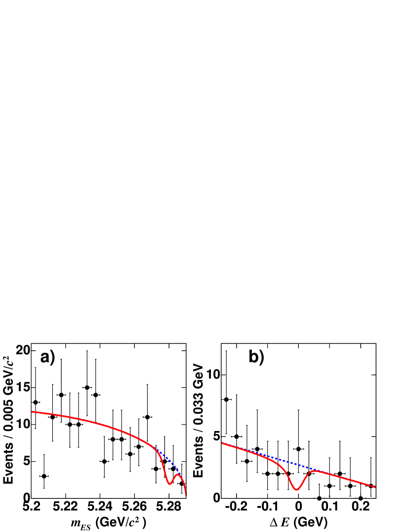
Figure 10: Distributions of the fit variables in $Ke\mu$ data (points), compared with projections of the combined fit (curves): (a) $m_{\rm ES}$ distribution after requiring $-0.11<\Delta E<0.05\ {\rm GeV}$ and (b) $\Delta E$ distribution after requiring $|m_{\rm ES}-m_{B}|<6.6\ {\rm MeV}/c^{2}$. The solid curve is the sum of all fit components, including signal; the dashed curve is the sum of all background components.

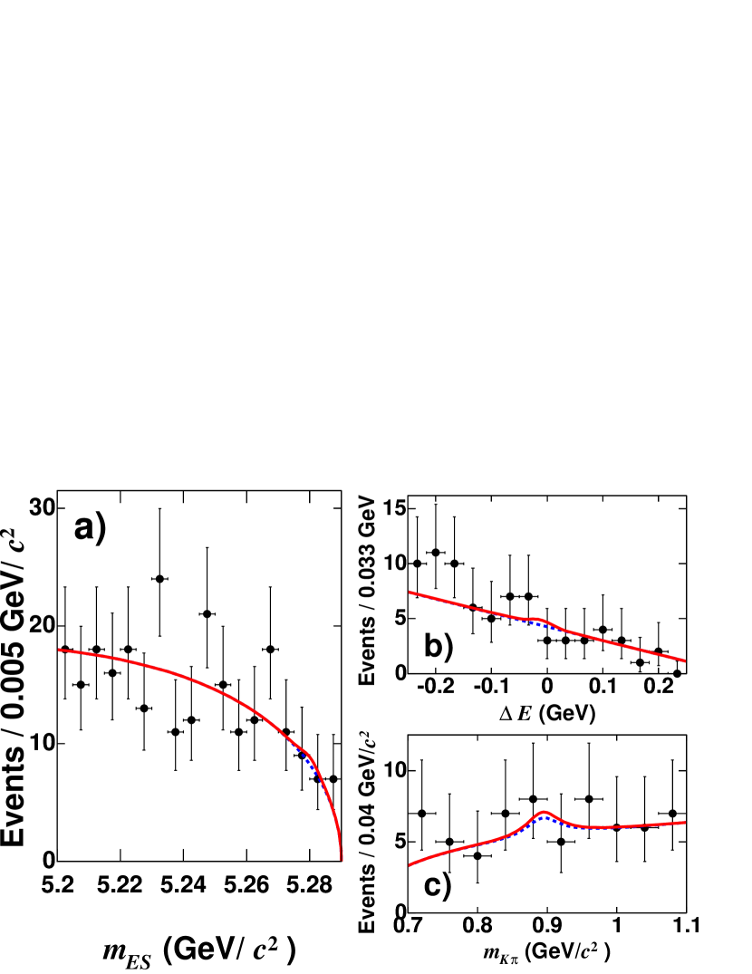
Figure 11: Distributions of the fit variables in $K^{*}e\mu$ data (points), compared with projections of the combined fit (curves): (a) $m_{ES}$ after requiring $-0.11<\Delta E<0.05\ {\rm GeV}$ and $0.817<m_{K\pi}<0.967\ {\rm GeV}/c^{2}$, (b) $\Delta E$ after requiring $|m_{\rm ES}-m_{B}|<6.6\ {\rm MeV}/c^{2}$, $0.817<m_{K\pi}<0.967\ {\rm GeV}/c^{2}$, and (c) $m_{K\pi}$ after requiring $|m_{\rm ES}-m_{B}|<6.6\ {\rm MeV}/c^{2}$ and $-0.11<\Delta E<0.05\ {\rm GeV}$. The solid curve is the sum of all fit components, including signal; the dashed curve is the sum of all background components.

VIII Conclusions

We have measured the branching fractions, partial branching fractions, direct $C\!P$ asymmetries, ratio of muons to electrons, fraction of longitudinal $K^{*}$ polarization, and lepton forward-backward asymmetries in the rare FCNC decays $B\rightarrow K\ell^{+}\ell^{-}$ and $B\rightarrow K^{*}\ell^{+}\ell^{-}$.

The branching fraction, $A_{C\!P}$, $R_{K}$, and $F_{L}$ results are all consistent with the Standard Model predictions for these decays. The values of $A_{FB}$ and the scalar contribution $F_{S}$ measured in the $B^{+}\rightarrow K^{+}\ell^{+}\ell^{-}$ channel are consistent with the expected value of zero. In the $B\rightarrow K^{*}\ell^{+}\ell^{-}$ channel the large positive value of $A_{FB}$ at high $q^{2}$ is consistent with the SM and disfavors new physics scenarios in which the relative sign of the product of the $C_{9}$ and $C_{10}$ Wilson coefficients is opposite that of the SM. At low $q^{2}$ a positive value of $A_{FB}$ is also favored, with a $95\%$ CL lower limit that is slightly above the SM prediction, as derived using the form factor models of Refs. bib:TheoryBc ; bib:TheoryE .

In addition, we have obtained upper limits on the lepton flavor-violating decays $B\rightarrow Ke\mu$ and $B\rightarrow K^{*}e\mu$ that are approximately one order of magnitude lower than those of previous searches.

We note that the Belle collaboration has recently reported bib:belleafb a measurement of the integrated forward-backward asymmetries, finding $\bar{A}_{FB}(B^{+}\rightarrow K^{+}\ell^{+}\ell^{-})=0.10\pm 0.14\pm 0.01$ and $\bar{A}_{FB}(B\rightarrow K^{*}\ell^{+}\ell^{-})=0.50\pm 0.15\pm 0.02$. From a fit to the $\cos\theta^{*}$ and $q^{2}$ distributions, they conclude that scenarios in which the product of $C_{9}$ and $C_{10}$ has the opposite sign as expected in the SM are disfavored, consistent with the results reported here.

All of the measurements reported here are limited by statistical uncertainties, and can be improved with the addition of more data.

IX Acknowledgments

We are grateful for the excellent luminosity and machine conditions provided by our PEP-II colleagues, and for the substantial dedicated effort from the computing organizations that support BABAR. The collaborating institutions wish to thank SLAC for its support and kind hospitality. This work is supported by DOE and NSF (USA), NSERC (Canada), IHEP (China), CEA and CNRS-IN2P3 (France), BMBF and DFG (Germany), INFN (Italy), FOM (The Netherlands), NFR (Norway), MIST (Russia), and PPARC (United Kingdom). Individuals have received support from CONACyT (Mexico), Marie Curie EIF (European Union), the A. P. Sloan Foundation, the Research Corporation, and the Alexander von Humboldt Foundation.

Appendix A Fits to angular distributions

In this appendix we present plots of the $\cos\theta_{K}$ and $\cos\theta^{*}$ distributions in data, together with the projections of the combined fits used to extract $F_{L}$ and $A_{FB}$. Figure 12 shows the fitted $\cos\theta_{K}$ distributions for each of the $q^{2}$ bins considered in this analysis. Figures 13 and 14 display the fitted $\cos\theta^{*}$ distributions for each of the $q^{2}$ ranges for the $B^{+}\rightarrow K^{+}\ell^{+}\ell^{-}$ and $B\rightarrow K^{*}\ell^{+}\ell^{-}$ decay modes, respectively. For the fits to the $\cos\theta^{*}$ distributions in the $B\rightarrow K^{*}\ell^{+}\ell^{-}$ mode, the $K^{*}$ polarization $F_{L}$ is fixed to its measured value, as described in the text. The deviations from a smooth parabolic shape in the signal component are the result of the efficiency and acceptance corrections, which are described by non-parametric histogram PDFs.

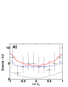
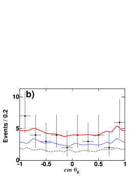
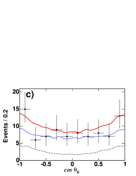
Figure 12: Distributions of the fit variable $\cos\theta_{K}$ in $B\rightarrow K^{*}\ell^{+}\ell^{-}$ data (points), compared with projections of the combined fit (curves) after requiring $-0.11<\Delta E<0.05\ {\rm GeV}$, $|m_{\rm ES}-m_{B}|<6.6\ {\rm MeV}/c^{2}$, and $0.817<m_{K\pi}<0.967\ {\rm GeV}/c^{2}$. The solid curve is the sum of all fit components, the dashed curve is the sum of all background components, and the dot-dashed curve is the signal component. The $q^{2}$ regions (a) $0.1<q^{2}<8.41\mathrm{\,Ge\kern-1.00006ptV}^{2}/c^{4}$, (b) $q^{2}>10.24\mathrm{\,Ge\kern-1.00006ptV}^{2}/c^{4}$, and (c) $q^{2}>0.1\mathrm{\,Ge\kern-1.00006ptV}^{2}/c^{4}$ are shown.

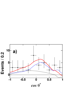
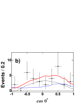
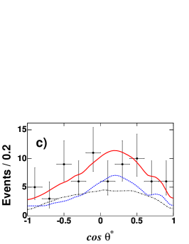
Figure 13: Distributions of the fit variable $\cos\theta^{*}$ in $B^{+}\rightarrow K^{+}\ell^{+}\ell^{-}$ data (points), compared with projections of the combined fit (curves) after requiring $-0.11<\Delta E<0.05\ {\rm GeV}$ and $|m_{\rm ES}-m_{B}|<6.6\ {\rm MeV}/c^{2}$. The solid curve is the sum of all fit components, the dashed curve is the sum of all background components, and the dot-dashed curve is the signal component. The $q^{2}$ regions (a) $0.1<q^{2}<8.41\mathrm{\,Ge\kern-1.00006ptV}^{2}/c^{4}$, (b) $q^{2}>10.24\mathrm{\,Ge\kern-1.00006ptV}^{2}/c^{4}$, and (c) $q^{2}>0.1\mathrm{\,Ge\kern-1.00006ptV}^{2}/c^{4}$ are shown. The combined fits shown for (a) and (b) are performed by fixing $F_{S}$ to zero.

References

(1)
G. Buchalla, A. J. Buras and M. E. Lautenbacher, Rev. Mod. Phys. 68, 1125 (1996).
(2) G. Burdman, Phys. Rev. D 52, 6400 (1995).
(3)JoAnne L. Hewett and J. D. Wells, Phys. Rev. D 55, 5549 (1997).
(4)
A. Ali, E. Lunghi, C. Greub, G. Hiller, Phys. Rev. D 66, 034002 (2002).
(5)
G. Eilam, J. L. Hewett, and T. G. Rizzo, Phys. Rev. D 34, 2773 (1986);
T. M. Aliev, A. Ozpineci, and M. Savci, Eur. Phys. J. C29, 265 (2003).
(6)
S. Davidson, D. C. Bailey, and B. A. Campbell, Z. Phys. C 61, 613 (1994).
(7)
P. Colangelo, F. DeFazio, P. Santorelli, E. Scrimieri, Phys. Rev. D
53, 3672 (1996).
(8)
P. Colangelo, F. DeFazio, P. Santorelli, E. Scrimieri, Phys. Rev. D
57, 3186(E) (1998).
(9)
A. Ali, P. Ball, L. T. Handoko, G. Hiller, Phys. Rev. D
61, 074024 (2000).
(10)
D. Melikhov, N. Nikitin, and S. Simula,
Phys. Rev. D 57, 6814 (1998).
(11)
T. M. Aliev et al., Phys. Lett. B 400,
194 (1997); T. M. Aliev, M. Savci, and A. Özpineci, Phys. Rev. D 56,
4260 (1997);
C. -H. Chen and C. Q. Geng, Phys. Rev. D 66, 094018 (2002);
H.-M. Choi, C. -R. Ji,
and L.S. Kisslinger, Phys. Rev. D 65, 074032 (2002);
N. G. Deshpande and J. Trampetic,
Phys. Rev. Lett. 60, 2583 (1988);
A. Faessler et al.,
EPJdirect C 4, 18 (2002);
C. Greub, A. Ioannissian, and D. Wyler, Phys. Lett. B 346, 149 (1995);
C. Q. Geng and C. P. Kao, Phys. Rev. D 54,
5636 (1996).
(12)
M. Zhong, Y.L. Wu, and W.Y. Wang, Int. J. Mod. Phys. A18, 1959 (2003).
(13)BABAR Collaboration, B. Aubert et al.,
Phys. Rev. Lett. 91, 221802 (2003).
(14)
Belle Collaboration, A. Ishikawa et al.,
Phys. Rev. Lett. 91, 261601 (2003).
(15)
F. Krüger, L. M. Sehgal, N. Sinha, and R. Sinha,
Phys. Rev. D 61, 114028 (2000); Erratum-ibid. D 63, 019901 (2001).
(16)
F. Krüger and E. Lunghi,
Phys. Rev. D 63, 014013 (2001).
(17)
G. Hiller and F. Krüger,
Phys. Rev. D 69, 074020 (2004).
(18)
Q. S. Yan, C. S. Huang, W. Liao, and S. H. Zhu,
Phys. Rev. D 62, 094023 (2000).
(19)
G. Buchalla, G. Hiller, and G. Isidori,
Phys. Rev. D 63, 014015 (2001).
(20)
D. A. Demir, K. A. Olive, and M. B. Voloshin,
Phys. Rev. D 66, 034015 (2002).
(21)
F. Krüger and J. Matias,
Phys. Rev. D 71, 094009 (2005).
(22)
C. Bobeth, T. Ewerth, F. Kruger, and J. Urban,
Phys. Rev. D 64 074014 (2001).
(23)BABAR Collaboration, B. Aubert et al., Nucl. Instrum. Methods A 479, 1 (2001).
(24)
P. Ball and R. Zwicky, Phys. Rev. D 71, 014015 (2005).
(25)
P. Ball and R. Zwicky, Phys. Rev. D 71, 014029 (2005).
(26)G. C. Fox and S. Wolfram, Phys. Rev. Lett. 41, 1581 (1978).
(27)R. A. Fisher, Ann. Eugenics 7, 179 (1936).
(28)BABAR Collaboration, B. Aubert et al.,
Phys. Rev. D 71, 032005 (2005).
(29)
Particle Data Group, S. Eidelman et al.,
Phys. Lett. B592, 1 (2004).
(30)
CLEO Collaboration, K. W. Edwards et al.,
Phys. Rev. D 65, 111102 (2002).
(31)BABAR Collaboration, B. Aubert et al.,
Phys. Rev. Lett. 88, 241801 (2002).
(32)
Belle Collaboration, A. Ishikawa et al.,
hep-ex/0603018, submitted to Phys. Rev. Lett.