CERN–PH-EP/2005-020

27 April 2005

DELPHI Collaboration

Abstract

An experimental study of the normalized three-jet rate of $b$ quark events with respect to light quarks events (light= $\ell\equiv u,d,s$) has been performed using the Cambridge and Durham jet algorithms. The data used were collected by the Delphi experiment at LEP on the $Z$ peak from 1994 to 2000. The results are found to agree with theoretical predictions treating mass corrections at next-to-leading order. Measurements of the $b$ quark mass have also been performed for both the $b$ pole mass: $M_{b}$ and the $b$ running mass: $m_{b}(M_{Z})$. Data are found to be better described when using the running mass. The measurement yields:

$$m_{b}(M_{Z})=2.85\pm 0.18~{}({\rm stat})\pm 0.13~{}({\rm exp})\pm 0.19~{}({\rm had})\pm 0.12~{}({\rm theo})~{}{\rm GeV}/c^{2}$$

for the Cambridge algorithm.

This result is the most precise measurement of the $b$ mass derived from a high energy process. When compared to other $b$ mass determinations by experiments at lower energy scales, this value agrees with the prediction of Quantum Chromodynamics for the energy evolution of the running mass. The mass measurement is equivalent to a test of the flavour independence of the strong coupling constant with an accuracy of 7$0$$\!/$$\!00$.

(Accepted by Euro. Phys. Journ. C)

J.Abdallah${}^{\ref{LPNHE}}$, P.Abreu${}^{\ref{LIP}}$, W.Adam${}^{\ref{VIENNA}}$, P.Adzic${}^{\ref{DEMOKRITOS}}$, T.Albrecht${}^{\ref{KARLSRUHE}}$, T.Alderweireld${}^{\ref{AIM}}$, R.Alemany-Fernandez${}^{\ref{CERN}}$, T.Allmendinger${}^{\ref{KARLSRUHE}}$, P.P.Allport${}^{\ref{LIVERPOOL}}$, U.Amaldi${}^{\ref{MILANO2}}$, N.Amapane${}^{\ref{TORINO}}$, S.Amato${}^{\ref{UFRJ}}$, E.Anashkin${}^{\ref{PADOVA}}$, A.Andreazza${}^{\ref{MILANO}}$, S.Andringa${}^{\ref{LIP}}$, N.Anjos${}^{\ref{LIP}}$, P.Antilogus${}^{\ref{LPNHE}}$, W-D.Apel${}^{\ref{KARLSRUHE}}$, Y.Arnoud${}^{\ref{GRENOBLE}}$, S.Ask${}^{\ref{LUND}}$, B.Asman${}^{\ref{STOCKHOLM}}$, J.E.Augustin${}^{\ref{LPNHE}}$, A.Augustinus${}^{\ref{CERN}}$, P.Baillon${}^{\ref{CERN}}$, A.Ballestrero${}^{\ref{TORINOTH}}$, P.Bambade${}^{\ref{LAL}}$, R.Barbier${}^{\ref{LYON}}$, D.Bardin${}^{\ref{JINR}}$, G.J.Barker${}^{\ref{KARLSRUHE}}$, A.Baroncelli${}^{\ref{ROMA3}}$, M.Battaglia${}^{\ref{CERN}}$, M.Baubillier${}^{\ref{LPNHE}}$, K-H.Becks${}^{\ref{WUPPERTAL}}$, M.Begalli${}^{\ref{BRASIL}}$, A.Behrmann${}^{\ref{WUPPERTAL}}$, E.Ben-Haim${}^{\ref{LAL}}$, N.Benekos${}^{\ref{NTU-ATHENS}}$, A.Benvenuti${}^{\ref{BOLOGNA}}$, C.Berat${}^{\ref{GRENOBLE}}$, M.Berggren${}^{\ref{LPNHE}}$, L.Berntzon${}^{\ref{STOCKHOLM}}$, D.Bertrand${}^{\ref{AIM}}$, M.Besancon${}^{\ref{SACLAY}}$, N.Besson${}^{\ref{SACLAY}}$, D.Bloch${}^{\ref{CRN}}$, M.Blom${}^{\ref{NIKHEF}}$, M.Bluj${}^{\ref{WARSZAWA}}$, M.Bonesini${}^{\ref{MILANO2}}$, M.Boonekamp${}^{\ref{SACLAY}}$, P.S.L.Booth${}^{\ref{LIVERPOOL}}$, G.Borisov${}^{\ref{LANCASTER}}$, O.Botner${}^{\ref{UPPSALA}}$, B.Bouquet${}^{\ref{LAL}}$, T.J.V.Bowcock${}^{\ref{LIVERPOOL}}$, I.Boyko${}^{\ref{JINR}}$, M.Bracko${}^{\ref{SLOVENIJA}}$, R.Brenner${}^{\ref{UPPSALA}}$, E.Brodet${}^{\ref{OXFORD}}$, P.Bruckman${}^{\ref{KRAKOW1}}$, J.M.Brunet${}^{\ref{CDF}}$, P.Buschmann${}^{\ref{WUPPERTAL}}$, M.Calvi${}^{\ref{MILANO2}}$, T.Camporesi${}^{\ref{CERN}}$, V.Canale${}^{\ref{ROMA2}}$, F.Carena${}^{\ref{CERN}}$, N.Castro${}^{\ref{LIP}}$, F.Cavallo${}^{\ref{BOLOGNA}}$, M.Chapkin${}^{\ref{SERPUKHOV}}$, Ph.Charpentier${}^{\ref{CERN}}$, P.Checchia${}^{\ref{PADOVA}}$, R.Chierici${}^{\ref{CERN}}$, P.Chliapnikov${}^{\ref{SERPUKHOV}}$, J.Chudoba${}^{\ref{CERN}}$, S.U.Chung${}^{\ref{CERN}}$, K.Cieslik${}^{\ref{KRAKOW1}}$, P.Collins${}^{\ref{CERN}}$, R.Contri${}^{\ref{GENOVA}}$, G.Cosme${}^{\ref{LAL}}$, F.Cossutti${}^{\ref{TU}}$, M.J.Costa${}^{\ref{VALENCIA}}$, D.Crennell${}^{\ref{RAL}}$, J.Cuevas${}^{\ref{OVIEDO}}$, J.D’Hondt${}^{\ref{AIM}}$, J.Dalmau${}^{\ref{STOCKHOLM}}$, T.da Silva${}^{\ref{UFRJ}}$, W.Da Silva${}^{\ref{LPNHE}}$, G.Della Ricca${}^{\ref{TU}}$, A.De Angelis${}^{\ref{TU}}$, W.De Boer${}^{\ref{KARLSRUHE}}$, C.De Clercq${}^{\ref{AIM}}$, B.De Lotto${}^{\ref{TU}}$, N.De Maria${}^{\ref{TORINO}}$, A.De Min${}^{\ref{PADOVA}}$, L.de Paula${}^{\ref{UFRJ}}$, L.Di Ciaccio${}^{\ref{ROMA2}}$, A.Di Simone${}^{\ref{ROMA3}}$, K.Doroba${}^{\ref{WARSZAWA}}$, J.Drees${}^{\ref{WUPPERTAL},\ref{CERN}}$, G.Eigen${}^{\ref{BERGEN}}$, T.Ekelof${}^{\ref{UPPSALA}}$, M.Ellert${}^{\ref{UPPSALA}}$, M.Elsing${}^{\ref{CERN}}$, M.C.Espirito Santo${}^{\ref{LIP}}$, G.Fanourakis${}^{\ref{DEMOKRITOS}}$, D.Fassouliotis${}^{\ref{DEMOKRITOS},\ref{ATHENS}}$, M.Feindt${}^{\ref{KARLSRUHE}}$, J.Fernandez${}^{\ref{SANTANDER}}$, A.Ferrer${}^{\ref{VALENCIA}}$, F.Ferro${}^{\ref{GENOVA}}$, U.Flagmeyer${}^{\ref{WUPPERTAL}}$, H.Foeth${}^{\ref{CERN}}$, E.Fokitis${}^{\ref{NTU-ATHENS}}$, F.Fulda-Quenzer${}^{\ref{LAL}}$, J.Fuster${}^{\ref{VALENCIA}}$, M.Gandelman${}^{\ref{UFRJ}}$, C.Garcia${}^{\ref{VALENCIA}}$, Ph.Gavillet${}^{\ref{CERN}}$, E.Gazis${}^{\ref{NTU-ATHENS}}$, R.Gokieli${}^{\ref{CERN},\ref{WARSZAWA}}$, B.Golob${}^{\ref{SLOVENIJA}}$, G.Gomez-Ceballos${}^{\ref{SANTANDER}}$, P.Goncalves${}^{\ref{LIP}}$, E.Graziani${}^{\ref{ROMA3}}$, G.Grosdidier${}^{\ref{LAL}}$, K.Grzelak${}^{\ref{WARSZAWA}}$, J.Guy${}^{\ref{RAL}}$, C.Haag${}^{\ref{KARLSRUHE}}$, A.Hallgren${}^{\ref{UPPSALA}}$, K.Hamacher${}^{\ref{WUPPERTAL}}$, K.Hamilton${}^{\ref{OXFORD}}$, S.Haug${}^{\ref{OSLO}}$, F.Hauler${}^{\ref{KARLSRUHE}}$, V.Hedberg${}^{\ref{LUND}}$, M.Hennecke${}^{\ref{KARLSRUHE}}$, H.Herr${}^{\ref{CERN}}$, J.Hoffman${}^{\ref{WARSZAWA}}$, S-O.Holmgren${}^{\ref{STOCKHOLM}}$, P.J.Holt${}^{\ref{CERN}}$, M.A.Houlden${}^{\ref{LIVERPOOL}}$, K.Hultqvist${}^{\ref{STOCKHOLM}}$, J.N.Jackson${}^{\ref{LIVERPOOL}}$, G.Jarlskog${}^{\ref{LUND}}$, P.Jarry${}^{\ref{SACLAY}}$, D.Jeans${}^{\ref{OXFORD}}$, E.K.Johansson${}^{\ref{STOCKHOLM}}$, P.D.Johansson${}^{\ref{STOCKHOLM}}$, P.Jonsson${}^{\ref{LYON}}$, C.Joram${}^{\ref{CERN}}$, L.Jungermann${}^{\ref{KARLSRUHE}}$, F.Kapusta${}^{\ref{LPNHE}}$, S.Katsanevas${}^{\ref{LYON}}$, E.Katsoufis${}^{\ref{NTU-ATHENS}}$, G.Kernel${}^{\ref{SLOVENIJA}}$, B.P.Kersevan${}^{\ref{CERN},\ref{SLOVENIJA}}$, U.Kerzel${}^{\ref{KARLSRUHE}}$, B.T.King${}^{\ref{LIVERPOOL}}$, N.J.Kjaer${}^{\ref{CERN}}$, P.Kluit${}^{\ref{NIKHEF}}$, P.Kokkinias${}^{\ref{DEMOKRITOS}}$, C.Kourkoumelis${}^{\ref{ATHENS}}$, O.Kouznetsov${}^{\ref{JINR}}$, Z.Krumstein${}^{\ref{JINR}}$, M.Kucharczyk${}^{\ref{KRAKOW1}}$, J.Lamsa${}^{\ref{AMES}}$, G.Leder${}^{\ref{VIENNA}}$, F.Ledroit${}^{\ref{GRENOBLE}}$, L.Leinonen${}^{\ref{STOCKHOLM}}$, R.Leitner${}^{\ref{NC}}$, J.Lemonne${}^{\ref{AIM}}$, V.Lepeltier${}^{\ref{LAL}}$, T.Lesiak${}^{\ref{KRAKOW1}}$, W.Liebig${}^{\ref{WUPPERTAL}}$, D.Liko${}^{\ref{VIENNA}}$, A.Lipniacka${}^{\ref{STOCKHOLM}}$, J.H.Lopes${}^{\ref{UFRJ}}$, J.M.Lopez${}^{\ref{OVIEDO}}$, D.Loukas${}^{\ref{DEMOKRITOS}}$, P.Lutz${}^{\ref{SACLAY}}$, L.Lyons${}^{\ref{OXFORD}}$, J.MacNaughton${}^{\ref{VIENNA}}$, A.Malek${}^{\ref{WUPPERTAL}}$, S.Maltezos${}^{\ref{NTU-ATHENS}}$, F.Mandl${}^{\ref{VIENNA}}$, J.Marco${}^{\ref{SANTANDER}}$, R.Marco${}^{\ref{SANTANDER}}$, B.Marechal${}^{\ref{UFRJ}}$, M.Margoni${}^{\ref{PADOVA}}$, J-C.Marin${}^{\ref{CERN}}$, C.Mariotti${}^{\ref{CERN}}$, A.Markou${}^{\ref{DEMOKRITOS}}$, C.Martinez-Rivero${}^{\ref{SANTANDER}}$, J.Masik${}^{\ref{FZU}}$, N.Mastroyiannopoulos${}^{\ref{DEMOKRITOS}}$, F.Matorras${}^{\ref{SANTANDER}}$, C.Matteuzzi${}^{\ref{MILANO2}}$, F.Mazzucato${}^{\ref{PADOVA}}$, M.Mazzucato${}^{\ref{PADOVA}}$, R.Mc Nulty${}^{\ref{LIVERPOOL}}$, C.Meroni${}^{\ref{MILANO}}$, E.Migliore${}^{\ref{TORINO}}$, W.Mitaroff${}^{\ref{VIENNA}}$, U.Mjoernmark${}^{\ref{LUND}}$, T.Moa${}^{\ref{STOCKHOLM}}$, M.Moch${}^{\ref{KARLSRUHE}}$, K.Moenig${}^{\ref{CERN},\ref{DESY}}$, R.Monge${}^{\ref{GENOVA}}$, J.Montenegro${}^{\ref{NIKHEF}}$, D.Moraes${}^{\ref{UFRJ}}$, S.Moreno${}^{\ref{LIP}}$, P.Morettini${}^{\ref{GENOVA}}$, U.Mueller${}^{\ref{WUPPERTAL}}$, K.Muenich${}^{\ref{WUPPERTAL}}$, M.Mulders${}^{\ref{NIKHEF}}$, L.Mundim${}^{\ref{BRASIL}}$, W.Murray${}^{\ref{RAL}}$, B.Muryn${}^{\ref{KRAKOW2}}$, G.Myatt${}^{\ref{OXFORD}}$, T.Myklebust${}^{\ref{OSLO}}$, M.Nassiakou${}^{\ref{DEMOKRITOS}}$, F.Navarria${}^{\ref{BOLOGNA}}$, K.Nawrocki${}^{\ref{WARSZAWA}}$, R.Nicolaidou${}^{\ref{SACLAY}}$, M.Nikolenko${}^{\ref{JINR},\ref{CRN}}$, A.Oblakowska-Mucha${}^{\ref{KRAKOW2}}$, V.Obraztsov${}^{\ref{SERPUKHOV}}$, A.Olshevski${}^{\ref{JINR}}$, A.Onofre${}^{\ref{LIP}}$, R.Orava${}^{\ref{HELSINKI}}$, K.Osterberg${}^{\ref{HELSINKI}}$, A.Ouraou${}^{\ref{SACLAY}}$, A.Oyanguren${}^{\ref{VALENCIA}}$, M.Paganoni${}^{\ref{MILANO2}}$, S.Paiano${}^{\ref{BOLOGNA}}$, J.P.Palacios${}^{\ref{LIVERPOOL}}$, H.Palka${}^{\ref{KRAKOW1}}$, Th.D.Papadopoulou${}^{\ref{NTU-ATHENS}}$, L.Pape${}^{\ref{CERN}}$, C.Parkes${}^{\ref{GLASGOW}}$, F.Parodi${}^{\ref{GENOVA}}$, U.Parzefall${}^{\ref{CERN}}$, A.Passeri${}^{\ref{ROMA3}}$, O.Passon${}^{\ref{WUPPERTAL}}$, L.Peralta${}^{\ref{LIP}}$, V.Perepelitsa${}^{\ref{VALENCIA}}$, A.Perrotta${}^{\ref{BOLOGNA}}$, A.Petrolini${}^{\ref{GENOVA}}$, J.Piedra${}^{\ref{SANTANDER}}$, L.Pieri${}^{\ref{ROMA3}}$, F.Pierre${}^{\ref{SACLAY}}$, M.Pimenta${}^{\ref{LIP}}$, E.Piotto${}^{\ref{CERN}}$, T.Podobnik${}^{\ref{SLOVENIJA}}$, V.Poireau${}^{\ref{CERN}}$, M.E.Pol${}^{\ref{BRASIL}}$, G.Polok${}^{\ref{KRAKOW1}}$, V.Pozdniakov${}^{\ref{JINR}}$, N.Pukhaeva${}^{\ref{AIM},\ref{JINR}}$, A.Pullia${}^{\ref{MILANO2}}$, J.Rames${}^{\ref{FZU}}$, A.Read${}^{\ref{OSLO}}$, P.Rebecchi${}^{\ref{CERN}}$, J.Rehn${}^{\ref{KARLSRUHE}}$, D.Reid${}^{\ref{NIKHEF}}$, R.Reinhardt${}^{\ref{WUPPERTAL}}$, P.Renton${}^{\ref{OXFORD}}$, F.Richard${}^{\ref{LAL}}$, J.Ridky${}^{\ref{FZU}}$, M.Rivero${}^{\ref{SANTANDER}}$, D.Rodriguez${}^{\ref{SANTANDER}}$, A.Romero${}^{\ref{TORINO}}$, P.Ronchese${}^{\ref{PADOVA}}$, P.Roudeau${}^{\ref{LAL}}$, T.Rovelli${}^{\ref{BOLOGNA}}$, V.Ruhlmann-Kleider${}^{\ref{SACLAY}}$, D.Ryabtchikov${}^{\ref{SERPUKHOV}}$, A.Sadovsky${}^{\ref{JINR}}$, L.Salmi${}^{\ref{HELSINKI}}$, J.Salt${}^{\ref{VALENCIA}}$, C.Sander${}^{\ref{KARLSRUHE}}$, A.Savoy-Navarro${}^{\ref{LPNHE}}$, U.Schwickerath${}^{\ref{CERN}}$, A.Segar${}^{\ref{OXFORD}}$, R.Sekulin${}^{\ref{RAL}}$, M.Siebel${}^{\ref{WUPPERTAL}}$, A.Sisakian${}^{\ref{JINR}}$, G.Smadja${}^{\ref{LYON}}$, O.Smirnova${}^{\ref{LUND}}$, A.Sokolov${}^{\ref{SERPUKHOV}}$, A.Sopczak${}^{\ref{LANCASTER}}$, R.Sosnowski${}^{\ref{WARSZAWA}}$, T.Spassov${}^{\ref{CERN}}$, M.Stanitzki${}^{\ref{KARLSRUHE}}$, A.Stocchi${}^{\ref{LAL}}$, J.Strauss${}^{\ref{VIENNA}}$, B.Stugu${}^{\ref{BERGEN}}$, M.Szczekowski${}^{\ref{WARSZAWA}}$, M.Szeptycka${}^{\ref{WARSZAWA}}$, T.Szumlak${}^{\ref{KRAKOW2}}$, T.Tabarelli${}^{\ref{MILANO2}}$, A.C.Taffard${}^{\ref{LIVERPOOL}}$, F.Tegenfeldt${}^{\ref{UPPSALA}}$, J.Timmermans${}^{\ref{NIKHEF}}$, L.Tkatchev${}^{\ref{JINR}}$, M.Tobin${}^{\ref{LIVERPOOL}}$, S.Todorovova${}^{\ref{FZU}}$, B.Tome${}^{\ref{LIP}}$, A.Tonazzo${}^{\ref{MILANO2}}$, P.Tortosa${}^{\ref{VALENCIA}}$, P.Travnicek${}^{\ref{FZU}}$, D.Treille${}^{\ref{CERN}}$, G.Tristram${}^{\ref{CDF}}$, M.Trochimczuk${}^{\ref{WARSZAWA}}$, C.Troncon${}^{\ref{MILANO}}$, M-L.Turluer${}^{\ref{SACLAY}}$, I.A.Tyapkin${}^{\ref{JINR}}$, P.Tyapkin${}^{\ref{JINR}}$, S.Tzamarias${}^{\ref{DEMOKRITOS}}$, V.Uvarov${}^{\ref{SERPUKHOV}}$, G.Valenti${}^{\ref{BOLOGNA}}$, P.Van Dam${}^{\ref{NIKHEF}}$, J.Van Eldik${}^{\ref{CERN}}$, N.van Remortel${}^{\ref{HELSINKI}}$, I.Van Vulpen${}^{\ref{CERN}}$, G.Vegni${}^{\ref{MILANO}}$, F.Veloso${}^{\ref{LIP}}$, W.Venus${}^{\ref{RAL}}$, P.Verdier${}^{\ref{LYON}}$, V.Verzi${}^{\ref{ROMA2}}$, D.Vilanova${}^{\ref{SACLAY}}$, L.Vitale${}^{\ref{TU}}$, V.Vrba${}^{\ref{FZU}}$, H.Wahlen${}^{\ref{WUPPERTAL}}$, A.J.Washbrook${}^{\ref{LIVERPOOL}}$, C.Weiser${}^{\ref{KARLSRUHE}}$, D.Wicke${}^{\ref{CERN}}$, J.Wickens${}^{\ref{AIM}}$, G.Wilkinson${}^{\ref{OXFORD}}$, M.Winter${}^{\ref{CRN}}$, M.Witek${}^{\ref{KRAKOW1}}$, O.Yushchenko${}^{\ref{SERPUKHOV}}$, A.Zalewska${}^{\ref{KRAKOW1}}$, P.Zalewski${}^{\ref{WARSZAWA}}$, D.Zavrtanik${}^{\ref{SLOVENIJA}}$, V.Zhuravlov${}^{\ref{JINR}}$, N.I.Zimin${}^{\ref{JINR}}$, A.Zintchenko${}^{\ref{JINR}}$, M.Zupan${}^{\ref{DEMOKRITOS}}$

1 Introduction

In $e^{+}e^{-}$ collisions, data collected at high energies are predominantly of hadronic nature showing a multi-jet final state topology. At LEP, these data have led to measurements of many of the Standard Model (SM) parameters and allowed limits to be set on new physics processes. In some cases the original quark flavour and its mass have not been a critical issue in performing the measurement and therefore approximations using massless quarks have been sufficient for the required precision. This is well justified for inclusive-type observables like total cross-sections for which the correction due to massive quarks depends on the quark mass, $m_{q}$, and on the energy of the process, $Q$, as $m_{q}^{2}c^{4}/Q^{2}$. For $b$ quarks ($m_{q}=m_{b}\sim 3-5$ GeV/$c^{2}$) at LEP I centre-of-mass energies ($Q=M_{Z}c^{2}$) this represents an effect of less than three per mille. On the other hand, for more exclusive observables, such as multi-jet cross-sections, the mass dependence transforms into terms proportional to $m_{q}^{2}c^{4}/(Q^{2}\cdot y_{c})$ where $y_{c}$, the jet resolution variable, usually takes values much lower than unity, enabling these mass effects to become sizeable [1]. Differences in the multi-jet production rate for massive $b$ quarks with respect to the corresponding rate for massless $\ell$ quarks ($\ell\equiv u,d,s$) can then be as large as 3% to 20% for three- or four-jet final states.

The large volume of data collected by the LEP experiments and the highly-effective techniques developed to identify the quark flavour of the jets, have increased the experimental sensitivity for observables where the quark flavour is relevant [2]. Consequently theoretical predictions including mass corrections have become necessary to reach a proper understanding of such observables in order to interpret them as standard or new physics. In some cases these mass effects have only been computed at leading order (LO) but for some event-shape variables and in particular for the three-jet rate, calculations including next-to-leading order (NLO) terms also exist [3, 4, 5, 6]. Rather precise experimental studies on the production of multi-jet events initiated by $b$ quarks have then been allowed and performed at LEP and SLC [7, 8, 9, 10, 11]. Results obtained agree well with the predictions of the Standard Model, i.e., Quantum Chromodynamics (QCD). The quantification of these mass effects has allowed a verification of the flavour independence of the strong coupling constant to a precision of less than 1% and an extraction of a value of the $b$ mass at the energy scale of the $Z$ boson mass, $Q=M_{Z}c^{2}$, within an uncertainty of $\sim 0.4-0.5$ GeV/$c^{2}$. These measurements have in addition provided the first evidence of the running of the $b$ mass, i.e. the evolution of this parameter as a function of the energy scale when compared to the values obtained from processes occuring at lower energy scales.

A reduction of the uncertainty of the $b$ mass determination could be accomplished by a combination of the present individual LEP and SLC results. This is certainly difficult and, at the end may improve the experimental precision only slightly, because the dominant errors are of systematic nature and common to all measurements. Hence, the best way to significantly increase the accuracy for this parameter is by a deeper understanding of the physics processes and correction procedures involved in the analyses.

1.1 The $b$ quark mass and the observable

The $b$ quark mass is a free parameter in the SM Lagrangian and therefore needs to be measured experimentally. Precise determinations of this parameter are very interesting both as a fundamental parameter and also to constrain models beyond the SM. Unfortunately, confinement of quarks inside the observed hadrons introduces additional complications not present in mass determinations of free particles as for instance leptons. Quark masses need then to be defined within a theoretical convention and can only be inferred indirectly through their influence on hadronic observables.

Among the different quark mass definitions, the most commonly used in high energy processes are the pole mass $M_{b}$ and the running mass $m_{b}(Q)$. The former is defined as the pole of the renormalized quark propagator and is gauge and scheme independent. The latter corresponds to the renormalized mass in the $\overline{\rm MS}$ scheme and depends on the process energy ($Q$). These mass definitions are related to each other [12] and NLO calculations are needed in order to distinguish between the two. Physics is independent of the mass definition. However, when using perturbation theory at a fixed order to extract physics results a dependence appears on the mass definition as well as on the arbitrary renormalization scale $\mu$. This is due to neglected perturbative and non-perturbative higher order terms and therefore it is possible than one scheme might be more convenient than another for a given purpose [13, 14]. Specially because the relation between the two mass definitions does not have a good convergence behaviour due to renormalon ambiguities [15].

In the case of the running mass $m_{b}(Q)$, the largest part of its running occurs at low energy scales up to $M_{Z}/2$. The exact mass running represents a basic constraint to theories beyond the SM, such as those implying the unification of the $b$ quark and $\tau$ lepton masses at the Grand Unified Theory (GUT) scale. The $b$ quark mass has also important implications on Higgs searches since the partial decay width of the Higgs boson into $b$ quarks is proportional to the $b$ quark mass squared. In this case, it can be shown that the mass definition is also relevant for the accuracy of the theoretical prediction [16, 17, 18].

At low energy, the $b$ quark mass is established from the measured spectra of hadronic bound states or the moments of the spectrum of the $B$ decay products making use of non-perturbative techniques such as the Heavy Quark Effective Theory (HQET), Non-Relativistic QCD (NRQCD), QCD sum rules or lattice QCD. An attempt to average these determinations properly is presented in [13] obtaining the value $m_{b}(m_{b})=4.24\pm 0.11$ GeV/$c^{2}$.

At high energy the $b$ quark mass has been extracted from data collected at the $Z$ peak at LEP and SLC. The first measurement of $m_{b}(M_{Z})$ was performed by the Delphi experiment with data collected from 1992 to 1994 at $\sqrt{s}\approx M_{Z}$. The observable used in this analysis was:

$$R_{3}^{b\ell}(y_{c})=\frac{R_{3}^{b}(y_{c})}{R_{3}^{\ell}(y_{c})}=\frac{\Gamma_{3j}^{b}(y_{c})/\Gamma^{b}}{\Gamma_{3j}^{\ell}(y_{c})/\Gamma^{\ell}}$$ (1)

with $\Gamma_{3j}^{q}(y_{c})$ and $\Gamma^{q}$ being, respectively, the three-jet and total decay widths of the $Z$ into $q\overline{q}$, where $q$ = $b$ or $\ell$ ($\ell\equiv u,d,s$ quarks). The flavour $q$ of the hadronic event was defined as that of the quarks coupling to the $Z$ and the Durham algorithm was used for the jet clustering. The measured observable was compared with the theoretical computations of [3] and $m_{b}$ in the $\overline{\rm MS}$ scheme was found to be [7]:

$$m_{b}(M_{Z})=2.67\pm 0.25~{}({\rm stat})\pm 0.34~{}({\rm had})\pm 0.27~{}({\rm theo})~{}{\rm GeV/}c^{2}$$ (2)

where the quoted error was mainly due to the hadronization uncertainty.

In this paper a new analysis to measure the $b$ mass, performed with data collected by Delphi from 1994 to 2000 is presented. The data taken in the years before have not been considered because the Vertex Detector layout was changed in 1994, improving its capability since then (see Section 2). The same observable as used in the previous Delphi measurement, $R_{3}^{b\ell}$, has been used with two jet-clustering algorithms, Cambridge [19] and Durham [20]. The Cambridge algorithm has the advantage of having a smaller theoretical uncertainty [6]. A detailed study of how mass effects and the hadronization process are implemented in the fragmentation models has led to a better control of the hadronization correction. The effect of the gluon-splitting rates into $b$ and $c$ quarks on the flavour tagging has also been taken into account.

2 The Delphi detector

A brief description of the most relevant components of the Delphi detector for this analysis is given here. A detailed description of its design and performance can be found in [21, 22].

Delphi was a hermetic detector with a superconducting solenoid providing a uniform magnetic field of 1.23 T parallel to the beam axis throughout the central tracking device volume.

The tracking system consisted of a silicon Vertex Detector (VD), a jet chamber Inner Detector (ID) and a Time Projection Chamber (TPC) which constituted the main tracking device in Delphi. At a larger distance from the interaction point the tracking was complemented by a drift chamber Outer Detector (OD) covering the barrel region ($40^{\circ}\leq\theta\leq 140^{\circ}$) and two sets of drift chambers, FCA and FCB, located in the endcaps.

The VD was made of three coaxial cylindrical layers of silicon strips. From 1994 onwards the outer and innermost layers were equiped with doubled-sided detectors with orthogonal strips, allowing the measurement of both $R\phi$ and $z$ coordinates. In 1996, the VD was doubled in length and in 1997 a Very Forward Detector consisting of ministrips and pixels was added. Earlier Delphi data taken in periods with a less complete VD setup are not included in this analysis whereas data collected, later, in the period of LEP2, 1996-2000, which corresponded to the calibration runs at the centre-of-mass energy of the $Z$ peak are used.

Electron and photon identification was provided mainly by the electromagnetic calorimeter which was composed of a High Density Projection Chamber (HPC) installed inside the coil in the barrel region and a lead-glass calorimeter (FEMC) in the forward region.

In order to measure the charged and neutral hadronic energy, Delphi also included the hadron calorimeter (HCAL), an iron-gas sampling detector incorporated in the magnet yoke.

3 Hadronization correction of $R_{3}^{b\ell}$

The hadronization correction to $R_{3}^{b\ell}$, i.e. the ratio of the observable at parton over hadron level, was computed in [7] using the string-fragmentation and cluster models implemented in Jetset 7.3 [23] and Herwig 5.8 [24] respectively, previously tuned to Delphi data [25]. Uncertainties coming from the tuned parameters of Jetset and from the different predictions of the two fragmentation models were taken into account, the latter being the highest contribution to the total error.

In the present analysis more recent versions of the generators in which $b$ quark mass effects are better modelled (Pythia 6.131 [26] and Herwig 6.1 [27]) were used. For the case of Pythia, different fragmentation functions were considered: Peterson [28] and Bowler [29] . The final hadronization correction applied to our observable was the one given by Pythia 6.131 with the Peterson $b$ fragmentation function since this model gives the best overall description of the Delphi data and the other two cases were only used to evaluate the model uncertainty.

The model uncertainty was reduced to a negligible effect by performing the measurement in a restricted region of the phase space. Other sources of uncertainties such as the effect of the $b$ quark mass parameter used in the generator were studied in detail and were shown also to be important. These two questions are discussed in the following sections.

3.1 Hadronization model uncertainty

The hadronization model uncertainty, $\sigma_{mod}$, was evaluated as the standard deviation of the hadronization corrections predicted by the cluster model implemented in Herwig and the string-fragmentation model of Pythia using two heavy quark fragmentation functions, Peterson and Bowler.

The hadronization corrections were found to depend on the $B$-hadron scaled energy, ${\rm x_{E}^{B}}=2E_{B-{\rm hadron}}/M_{Z}$, the distribution of which is shown in Figure 1. As this quantity and the corresponding jet energy including the $B$-hadron are highly correlated a new variable was defined instead: the $b$-jet scaled energy ${\rm x_{E}^{b}}({\rm jet})=2E_{b-\mathrm{jet}}/M_{Z}$ where $E_{b-\rm{jet}}$ is the energy of the jets originated by the primary $b$ quarks in a $Z\rightarrow b\overline{b}$ event. The study of the dependence of the hadronization corrections with ${\rm x_{E}^{b}}({\rm jet})$ led to the conclusion that if the cut ${\rm x_{E}^{b}}(\mathrm{jet})\geq 0.55$ is applied to both $b$ quark jets the model uncertainty is reduced by a factor of 4 (see the right hand plot in Figure 1 and Figure 2 ).

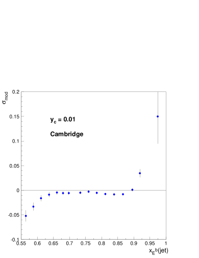
Figure 1: ${\rm x_{E}^{B}}$ distribution for the different Monte Carlo generators (left). Hadronization model uncertainty (i.e. standard deviation of the hadronization corrections predicted by Herwig and Pythia with Peterson and Bowler heavy fragmentation functions) as a function of the mean of the ${\rm x_{E}^{b}}({\rm jet})$ that is defined in the text and for $y_{c}=0.01$ for Cambridge (right).

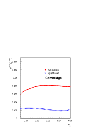
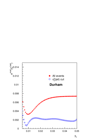
Figure 2: Hadronization model uncertainty as a function of the $y_{c}$ for the Cambridge (left) and Durham (right) algorithms.

3.2 The $b$ mass parameter in the generator

In this section, the effect of the $b$ quark mass parameter used in Pythia on the hadronization correction is discussed. The result of this study also applies to other generators which contain similar features.

In order to describe $b$ quark mass effects, Pythia uses a set of three $b$ quark mass parameters: the kinematical mass, $M_{b}^{kine}$, used in the parton shower (PS) process, the constituent mass, $M_{b}^{const}$, used during the hadronization process and finally the known $B$ hadron masses. The constituent mass is also used to derive masses for predicted but not yet observed $B$ hadrons. In the model these three masses are not connected to each other and, as a consequence, mass effects at parton level do not automatically propagate to the hadronization process, as they physically should. This results in a dependence of the hadronization correction on the $b$ quark mass of the generator.

If the various mass parameters are connected by, for instance, making the constituent and kinematical $b$ quark masses equal to each other and by deriving all $B$ hadron masses from the corresponding quark masses using the hadron mass formula [30], this dependence of the hadronization correction factor is completely removed. This feature of the generators was also noticed in previous studies [7, 8, 9, 10, 11] even though the exact cause of this behaviour was not identified. Unfortunately, this argument cannot define the value to be assigned to the mass parameters of the standard generator in which the quark masses are not connected. For that purpose, the following procedure was applied:

• In order to assess the precision of the massive calculation implicit in the parton shower generator, its prediction for $R_{3}^{b\ell}$ and that of the NLO calculation was first compared. The method was to change the input mass in the NLO calculations to minimize their overall difference. Then the difference of the input mass values was evaluated. For the parton shower the so called kinematical mass, $M_{b}^{kine}$, was employed and for the NLO calculations the two mass definitions were considered. In the case of the running mass the corresponding value was transformed to the pole mass . The value $\Delta(M_{b}^{kine}-M_{b})\sim 15$ MeV/$c^{2}$ was obtained in the case of the running mass and $\Delta(M_{b}^{kine}-M_{b})\sim 500$ MeV/$c^{2}$ for the pole mass. These differences were later considered as the uncertainty associated to the effective mass definition of the parton shower.

• The values of the $b$ quark mass measurements determined from low energy processes were then used as input to the mass parameter, $M_{b}^{kine}$, of the generator entering in the hadronization process. In order to select the mass value to be used in the present analysis, various possibilites were explored. A direct determination of $M_{b}$ from reference [31] gave $M_{b}=4.98\pm 0.13$ GeV/$c^{2}$. A second possibility is to use the average value for the running mass calculated in [13] as: $m_{b}(m_{b})=4.24\pm 0.11$ GeV/$c^{2}$, which could be transformed into a pole mass value of $M_{b}=4.99\pm 0.13$ GeV/$c^{2}$. A third value is also available using Delphi data from the semileptonic $B$ decays for which the relevant scale is that of the $B$ hadron masses, leading to $M_{b}=5.00\pm 0.16$ GeV/$c^{2}$ [34]. All these results are compatible and have similar accuracy. The value which was used in the generator to compute the hadronization correction was that obtained as the average of all low energy measurements [13]:

  $$m_{b}(m_{b})=4.24\pm 0.11\ {\rm GeV}/c^{2},\ \ {\rm or},\ \ M_{b}=4.99\pm 0.13\ {\rm GeV}/c^{2}.$$ (3)

For cross-check purposes, values of the $b$ quark mass were also extracted using Delphi data alone with the modified generator for which the set of the three $b$ quark masses are connected to each other. Two different observables were employed for this study: the $y_{32}$ distribution of $b$ over $\ell$ events normalized to the total number of $b$ and $\ell$ events, $R^{b\ell}(y_{32})$ and the minimum angle between $b$ quark and gluon jets when every event is forced to three jets. Both quantities are correlated with the observable $R_{3}^{b\ell}$ used to measure the $b$ quark mass and therefore their role in the present analysis is limited to qualitative checks. The first observable gave a fitted value for the $b$ quark mass of the modified generator of $M_{b}=4.93\pm 0.13$ GeV/$c^{2}$ and the second one $M_{b}=4.95\pm 0.11$ GeV/$c^{2}$. These results are thus consistent with the choice of the mass parameter and the above quoted uncertainty.

4 Experimental determination of $R_{3}^{b\ell}$

First the sample of $Z$ hadronic decays, i.e. $Z\rightarrow q\overline{q}$ events was selected. Then the $b$ and $\ell$ quark-initiated events were separated using the Delphi flavour tagging methods and later a cut on the $b$ quark jet energy was also performed in order to discard those events with large hadronization correction (see Section 3.1).

The jet-clustering algorithms Cambridge and Durham were applied to both tagged samples to obtain the $R_{3}^{b\ell}$ observable at detector level. Data were then corrected for detector and tagging effects and for the hadronization process to bring the observable to parton level.

4.1 Event selection

The selection of $Z$ hadronic events was done in three steps (as in [7]):

• particle selection: Charged and neutral particles were selected in order to ensure a reliable determination of their momenta and energies by applying the cuts listed in Table 1;

• event selection: $Z\rightarrow q\overline{q}$ events were selected by imposing the global event conditions of Table 1;

• kinematic selection: In order to reduce particle losses and imperfect energy-momentum assignment to jets in the selected hadronic events, further kinematical cuts were applied. Each event was clustered into three jets by the jet-clustering algorithm (Cambridge and Durham) using all selected charged and neutral particles. The cuts of Table 1 were then applied.

After applying these cuts to the data a sample of $1.4\times 10^{6}$ ($1.3\times 10^{6}$) hadronic $Z$ decays was selected for the Cambridge (Durham) algorithm.

	$p\geq$ 0.1 GeV/$c$
Charged	25${}^{\circ}\leq\theta\leq 155^{\circ}$
Particle	L$\geq$ 50 cm
Selection	$d\leq$ 5 cm in $R\phi$ plane
	$d\leq$ 10 cm in $z$ direction
Neutral	$E\geq 0.5$ GeV,  40∘ $\leq\theta\leq$ $140^{\circ}$ (HPC)
Cluster	$E\geq 0.5$ GeV,  8∘(144∘) $\leq\theta\leq$ $36^{\circ}$(172∘)       (FEMC)
Selection	$E\geq 1$ GeV,  10${}^{\circ}\leq\theta\leq 170^{\circ}$ (HCAL)
	$N_{ch}\geq 5$
	$E_{ch}\geq 15$ GeV
Event	$|\sum_{i}{q_{i}}|\leq 6$, $i=1,...,N_{ch}$
Selection	No charged particle with $p\geq 40$ GeV/$c$
	45${}^{\circ}\leq\theta_{thrust}\leq 135^{\circ}$
	$N^{ch}_{j}\geq 1$ per jet
Kinematic	$E_{j}\geq 1$ GeV,  $j=1,2,3$
Selection	25${}^{\circ}\leq\theta_{j}\leq 155^{\circ}$,  $j=1,2,3$
	Planarity cut: $\sum_{ij}{\phi_{ij}}\geq 359^{\circ},\ \ \ i<j,\ \ i,j=1,2,3$

Table 1: Particle and hadronic-event selection cuts; $p$ is the particle momentum, $\theta$ the particle polar angle and $\theta_{thrust}$ the $thrust$ polar angle (with respect to the beam axis in both cases), L the measured track length, $d$ the closest distance to the interaction point, $q_{i}$ the particle charge, $E$ the cluster energy, $N_{ch}$ the number of charged particles, and $E_{ch}$ the total charged-particle energy in the event. The kinematic selection is based on the properties of the events when clustered into three jets by the jet algorithm. $N^{ch}_{j}$ is the jet charged multiplicity, $E_{j}$ the jet energy, $\theta_{j}$ the jet polar angle and $\phi_{ij}$ the angular separation between the pair of jets $ij$.

4.2 Flavour tagging

The $b$ and light ($\ell\equiv u,d,s$) quark-initiated events need to be identified. Delphi has developed two different algorithms for $b$ tagging based on those properties of $B$ hadrons that differ from those of other particles: the impact parameter [35] and the combined technique [36]. The former makes use of the most important property for the selection of $B$ hadrons, their long lifetime, and discriminates the flavour of the event by calculating the probability, $P_{E}^{+}$, of having all particles compatible with being generated at the event interaction point. The second technique, besides the impact parameter of charged particles, uses other discriminating variables: the transverse momentum of any identified energetic lepton with respect to the jet direction and, in case a secondary vertex is found, the total invariant mass, the fraction of energy, the transverse momentum and the rapidities of the charged tracks belonging to the secondary vertex. An optimal combination of this set of variables defined for each reconstructed jet is performed, leading to a single variable per event, $X_{effev}$. When the aim was to measured $R_{3}^{b\ell}$ for Cambridge, this was also the algorithm used to compute the combined tagging variable, and the same for the case of Durham.

Figure 3 shows the distributions of $P_{E}^{+}$ and $X_{effev}$ obtained for the selected real and simulated sample of $Z$ hadronic decays. For the case of the simulated data, the contribution of each quark flavour is also indicated.

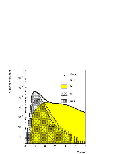
Figure 3: Event distribution of $P_{E}^{+}$ (left) and $X_{effev}$ (right) when Durham is used to form jets. The real (points) and simulated (histogram) data are compared. The specific contribution of each quark flavour is displayed as derived from the Delphi simulated data. The cuts used to tag the $b$ and $\ell$ quark sample are also indicated.

Taking into account the stability of the final result (see Figure 4 left), the impact parameter method was used for $\ell$ tagging by imposing $P_{E}^{+}>0.07$. The resulting purity of the sample and efficiency of the selection were $P_{\ell}=82$% and $\epsilon_{\ell}$ = 51%, respectively. For $b$ tagging both techniques were observed to be equally stable. The combined method was used requiring $X_{effev}>-0.15$ since higher purities could be reached for the same efficiency. The final purity of the sample and the total efficiency were $P_{b}=86$% and $\epsilon_{b}$ = 47%, respectively, where this efficiency value also takes into account the hadronic selection.

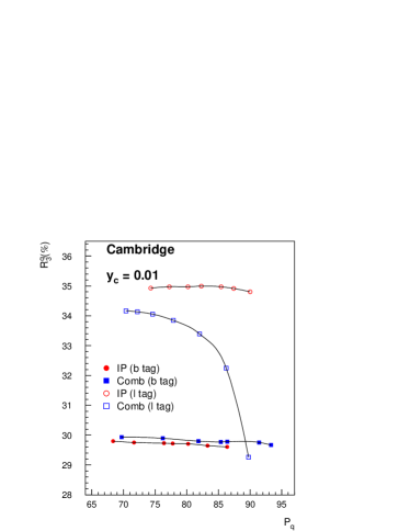
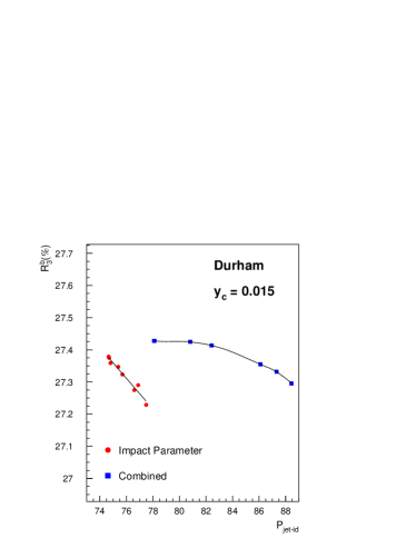
Figure 4: (Left) $R_{3}^{q}=\Gamma_{3j}^{q}(y_{c})/\Gamma^{q}$ at parton level as a function of the purity of the $q$-tagged sample, $P_{q}$, for $q=b,\ell$, when Cambridge is used to form jets. (Right) $R_{3}^{b}$ as a function of the jet identification purity for the Durham algorithm.

In order to perform the cut on the $b$ quark energies (see Section 3.1), an identification of the gluon and $b$ quark jets was required for $b$-tagged events. The two tagging techniques can also provide a discriminant variable per jet and therefore both are available for jet identification. Again, based on a stability argument (see Figure 4 right), the combined technique was used to identify the pair of jets most likely to come from $b$ quarks by requiring $X_{effev}>-0.5$ (where now $X_{effev}$ is only computed with the tracks contained in the pair of jets which gives the maximum $X_{effev}$). This results in a $b$ jet purity of 81% per jet in each event and a tag efficiency of 90%.

Once the $b$ quark jets were identified their energy was computed from the jet directions using energy-momentum conservation and assuming massless kinematics. Figure 5 shows the ${\rm x_{E}^{b}}(\mathrm{jet})$ distribution for real and simulated data. The cut ${\rm x_{E}^{b}}(\mathrm{jet})\geq 0.55$ was then applied for both $b$ jets. The purity and contamination factors of the $b$ and $\ell$-tagged samples obtained after the cut are shown in Table 2.

Figure 5: ${\rm x_{E}^{b}}(\mathrm{jet})$ distribution for real and simulated data for three-jet $b$-tagged events at $y_{c}=0.015$ for Cambridge.

Method	Type $q$	${\ell}\rightarrow q$ (%)	$c\rightarrow q$ (%)	$b\rightarrow q$ (%)
Impact Parameter	${\ell}$	82	15	3
Combined	$b$	2	7	91

Table 2: Flavour composition of the samples tagged as $\ell$ or $b$ quark events. $(\ell,c,b)\rightarrow q$ refers to the fraction of true $q^{\prime}$ events in the $q$-tagged sample.

4.3 Data correction

Once the $b$ and $\ell$ quark hadronic events were selected from the collected data, the jet-clustering algorithm was applied to get the $R_{3}^{b\ell}$ observable at detector level, $R_{3}^{b\ell-det}$. In order to bring the observable to parton level the method of the previous Delphi measurement was used [7]. A correction to obtain pure $b$ and $\ell$-quark samples was applied in this procedure and the flavour composition uncertainties were accounted for by the tagging uncertainty.

The Delphi full simulation (Delsim), which uses Jetset 7.3 to generate the events that go through the detector simulation, was used to compute the detector correction. A reweighting of the events was done in order to reproduce the measured heavy quark gluon-splitting rates [37] ($g_{c\overline{c}}=0.0296\pm 0.0038$ and $g_{b\overline{b}}=0.00254\pm 0.00051$) in the simulation.

A recent version of Pythia 6.131, tuned to Delphi data [25] and with the kinematical $b$ quark mass parameter set to $M_{b}=4.99\pm 0.13$ GeV/$c^{2}$, was used to get the hadronization correction.

The magnitude of the detector and hadronization corrections for $R_{3}^{b\ell}$ are shown in Figure 6. At the $y_{c}$ value chosen for the final result ($y_{c}=0.0085$ and $y_{c}=0.02$ for Cambridge and Durham, respectively) the detector correction is about -2.5% for Durham and 5$0$$\!/$$\!00$   for Cambridge. The hadronization correction is 1% for Cambridge and half as big for Durham.

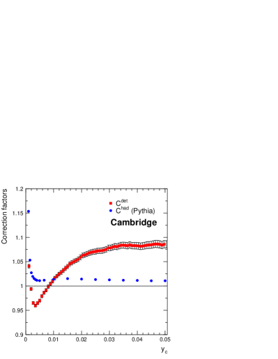
Figure 6: Detector and hadronization corrections applied to the measured $R_{3}^{b\ell}$ for Cambridge and Durham. The detector correction, $C^{det}$, brings the observable to hadron level, and the hadronization correction, $C^{had}$, brings it from this stage to parton level.

4.4 Experimental uncertainties

Apart from the statistical uncertainties, different sources of systematic uncertainties were considered. They can be divided into two groups: those due to the hadronization correction and those due to the detector correction.

• hadronization:

  The following sources of uncertainties in the hadronization correction have been taken into account:

  • uncertainty in the tuned parameters of Pythia that are relevant in the fragmentation process. This contribution was evaluated by varying these parameters ($\Lambda_{\mathrm{QCD}}$, $Q_{0}$, $\sigma_{q}$, $\epsilon_{b}$, $a$) within $\pm 1$ standard deviation around their tuned central values, taking into account correlations [25];

  • uncertainty due to the choice of the hadronization model. It was calculated as the standard deviation of the three hadronization models used (see Section 3.1);

  • uncertainty from varying the value of the $b$ quark mass parameter in the generator within the error of 0.13 GeV/$c^{2}$ about its chosen central value of $M_{b}$ = 4.99 GeV/$c^{2}$ (see Section 3.2).

• detector:

  The uncertainties in the detector correction, including selection efficiencies, acceptance effects and the tagging procedure, are due to imperfections in the physics and detector modelling provided in the simulation. The following sources were considered:

  • gluon-splitting: The measured $c\overline{c}$ and $b\overline{b}$ gluon-splitting rates were varied within their uncertainty and the effect on the measured observable was taken as the gluon-splitting error;

  • tagging: The related uncertainty was evaluated by varying the tagging and mis-tagging efficiencies within their uncertainties: $\Delta\epsilon_{b}^{b}/\epsilon_{b}^{b}=3$% and $\Delta\epsilon_{b}^{\ell}/\epsilon_{b}^{\ell}=\Delta\epsilon_{b}^{c}/\epsilon_{b}^{c}=8$% evaluated as in [38] (being $\epsilon_{q}^{q^{\prime}}$ the fraction of $q^{\prime}$ tagged events in the true $q$-quark sample). For this purpose, $\ell$ tagging was considered equivalent to anti-$b$ tagging, i.e. $\Delta\epsilon_{\ell}^{q}=\Delta\epsilon_{b}^{q}$ for $q=b,c,\ell$ for the same cut value;

  • jet identification: The cut applied to distinguish the $b$ quark jets from the gluon jet in a $b$ tagged event was varied in order to obtain cut efficiencies (i.e. the fraction of events which pass the cut applied to select the two $b$ quark jets among the 3 jets) between 80% and almost 100%. Half of the full variation observed in the measured $R_{3}^{b\ell}$ at parton level was taken as the uncertainty due to the jet identification.

4.5 Results for $R_{3}^{b\ell}$ at hadron and parton level

Figure 7 shows, as a function of the $y_{c}$, the measured $R_{3}^{b\ell}$ corrected to hadron level together with the curves predicted by the Pythia and Herwig generators. The statistical-only and total uncertainties can also be seen in this figure. The Pythia curves are shown independently for the Peterson and Bowler $b$ fragmentation functions. For large values of $y_{c}$, both generators describe the data well. The measured $R_{3}^{b\ell}$ ratio and its uncertainties are also presented in Tables 3 and 4.

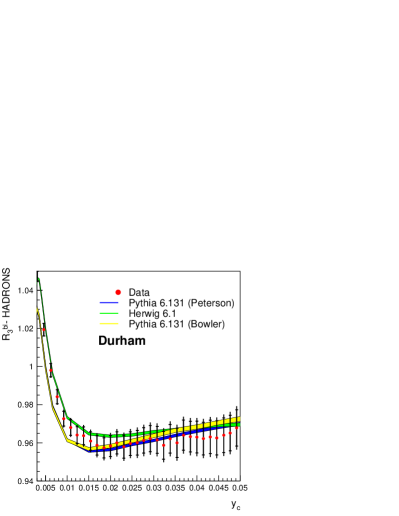
Figure 7: $R_{3}^{b\ell}$ at hadron level as a function of $y_{c}$ compared with Pythia 6.131 (with Peterson and Bowler fragmentation $b$ functions) and Herwig 6.1 predictions, using the Cambridge (left) and Durham (right) jet-clustering algorithms.

The result for $R_{3}^{b\ell}$ obtained at parton level is shown in Figure 8 as a function of $y_{c}$ together with its statistical and total uncertainties. The LO and NLO theoretical predictions in terms of the pole and running masses ($M_{b}=4.99$ GeV/$c^{2}$ and $m_{b}(M_{Z})=2.91$ GeV/$c^{2}$) are also shown in the plot. In the case of Cambridge the LO prediction is already reproducing the measured data, indicating a better convergence in the theoretical calculations than for Durham. The results for the individual years of data taking are compatible (see Figure 9).

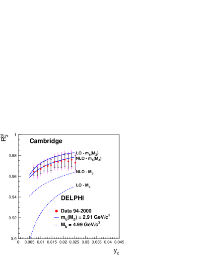
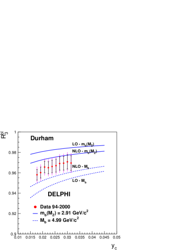
Figure 8: $R_{3}^{b\ell}$ as a function of $y_{c}$ obtained at parton level compared with the LO and NLO theoretical predictions calculated in terms of a pole mass of $M_{b}=4.99$ GeV/$c^{2}$ and in terms of a running mass of $m_{b}(M_{Z})=2.91$ GeV/$c^{2}$.

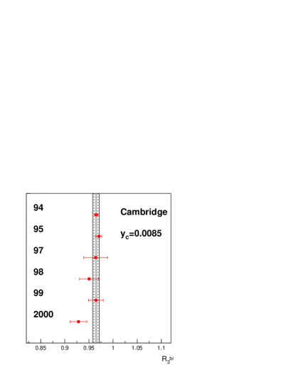
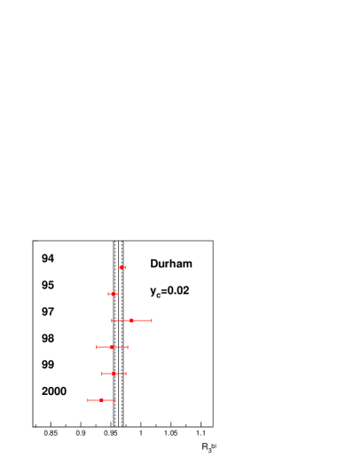
Figure 9: $R_{3}^{b\ell}$ at parton level obtained for each analysed year for a fixed $y_{c}$ for Cambridge (left) and Durham (right). The error bars represent the statistical error. The vertical lines show the average value with its statistical and total error. The $\chi^{2}$ per degree of freedom of the average is 0.7 and 1.2 for Cambridge and Durham respectively.

$y_{c}$	$R_{3}^{b\ell-had}$	$\sigma_{stat}$	$\sigma_{g-splitting}$	$\sigma_{tag}$	$\sigma_{jet-id}$
0.005	0.9617	$\pm$0.0034	$\pm$0.0003	$\pm$0.0014	$\pm$0.0016
0.01	0.9544	$\pm$0.0044	$\pm$0.0010	$\pm$0.0025	$\pm$0.0019
0.015	0.9560	$\pm$0.0052	$\pm$0.0014	$\pm$0.0031	$\pm$0.0021
0.02	0.9632	$\pm$0.0059	$\pm$0.0018	$\pm$0.0036	$\pm$0.0024
0.025	0.9639	$\pm$0.0067	$\pm$0.0021	$\pm$0.0039	$\pm$0.0026
0.03	0.9629	$\pm$0.0074	$\pm$0.0024	$\pm$0.0041	$\pm$0.0029

Table 3: $R_{3}^{b\ell}$ at hadron level at different $y_{c}$ with jets reconstructed with Cambridge.

$y_{c}$	$R_{3}^{b\ell-had}$	$\sigma_{stat}$	$\sigma_{g-splitting}$	$\sigma_{tag}$	$\sigma_{jet-id}$
0.005	1.0194	$\pm$0.0033	$\pm$0.0002	$\pm$0.0011	$\pm$0.0008
0.01	0.9690	$\pm$0.0039	$\pm$0.0007	$\pm$0.0025	$\pm$0.0010
0.015	0.9613	$\pm$0.0047	$\pm$0.0012	$\pm$0.0031	$\pm$0.0012
0.02	0.9583	$\pm$0.0056	$\pm$0.0016	$\pm$0.0036	$\pm$0.0014
0.025	0.9596	$\pm$0.0062	$\pm$0.0018	$\pm$0.0040	$\pm$0.0015
0.03	0.9611	$\pm$0.0070	$\pm$0.0022	$\pm$0.0043	$\pm$0.0017
0.035	0.9606	$\pm$0.0076	$\pm$0.0025	$\pm$0.0045	$\pm$0.0019
0.04	0.9630	$\pm$0.0083	$\pm$0.0027	$\pm$0.0046	$\pm$0.0021
0.045	0.9626	$\pm$0.0089	$\pm$0.0029	$\pm$0.0048	$\pm$0.0022
0.05	0.9687	$\pm$0.0097	$\pm$0.0032	$\pm$0.0050	$\pm$0.0024

Table 4: $R_{3}^{b\ell}$ at hadron level at different $y_{c}$ with jets reconstructed with Durham.

5 Comparison with NLO massive calculations

The measurement of the $R_{3}^{b\ell}$ observable at parton level obtained in the previous section, when compared with the NLO massive calculations of [3, 6], can be used either to extract the $b$ quark mass assuming $\alpha_{s}$ universality or to test $\alpha_{s}$ flavour independence taking the $b$ quark mass measured at threshold as an input.

5.1 Determination of the $b$ quark mass

In order to extract the $b$ quark mass from the experimentally measured $R_{3}^{b\ell}$, a value of $y_{c}$ must be chosen for both Cambridge and Durham jet algorithms. The value used was that which gave the smallest overall uncertainty on the measurement while staying in the region where the hadronization correction remains flat. In this way it was also guaranteed to keep far enough from the four-jet region. The selected values found to best fulfill these requirements were $y_{c}=0.0085$ and $y_{c}=0.02$ for Cambridge and Durham, respectively, where the four-jet rates are 4-5$\%$ and 2-3$\%$ in each case.

The $b$ quark pole mass, $M_{b}$, could be extracted from the measured $R_{3}^{b\ell}$ using the NLO expression of $R_{3}^{b\ell}$ in terms of $M_{b}$ [3, 6]. Theoretical sources of uncertainty were the $\mu$ scale dependence, the identification of the $b$ quark mass parameter in the generator (see Section 3.2) and $\alpha_{s}$.

The measured $b$ quark pole mass was found to be,

$$M_{b}=4.19\pm 0.23~{}({\rm stat})\pm 0.17~{}({\rm exp})\pm 0.25~{}({\rm had})^{+0.70}_{-0.83}~{}({\rm theo})~{}{\rm GeV/c^{2}}$$ (4)

when Cambridge is used to reconstruct jets with $y_{c}=0.0085$ and,

$$M_{b}=4.47\pm 0.31~{}({\rm stat})\pm 0.24~{}({\rm exp})\pm 0.24~{}({\rm had})^{+0.64}_{-0.76}~{}({\rm theo})~{}{\rm GeV/c^{2}}$$ (5)

when Durham is used instead with $y_{c}=0.02$. Although compatible within errors, these values are low compared with the results obtained when the $b$ pole mass is measured at low energy (as for example 4.98 $\pm$ 0.13 GeV/$c^{2}$ [31]). The measurement error is dominated by the uncertainty from the identification of the $b$ quark mass parameter in the generator with the $b$ pole mass which contributes to the theoretical error.

The running mass was also obtained using the NLO computations of $R_{3}^{b\ell}$ from references [3, 6], in this case, in terms of the running mass at the $M_{Z}$ energy scale: $m_{b}(M_{Z})$. The theoretical uncertainty was estimated by considering the following sources:

• dependence on the renormalization scale: The $\mu$ scale in the theoretical expressions was varied from $M_{Z}/2$ to $2M_{Z}$ and half of the difference between the result obtained on $m_{b}(M_{Z})$ was taken as the $\mu$ scale error;

• mass ambiguity: Starting from the NLO calculation of $R_{3}^{b\ell}$ in terms of the pole mass $M_{b}$, the value of $M_{b}$ could be extracted and transformed to $m_{b}(M_{b})$ which was later evolved to $m_{b}(M_{Z})$ by means of the Renormalization Group Equations. This is also a valid procedure to extract $m_{b}(M_{Z})$. At infinite orders the result derived in this way and that obtained directly from the original NLO calculation in terms of the running mass should be the same. The difference between the results obtained from the two procedures was then also considered as a conservative indication of the size of the unknown higher order corrections;

• $\alpha_{s}$: $\alpha_{s}(M_{Z})=0.1183\pm 0.0027$ [33] was varied within its uncertainty. The spread of values obtained for $m_{b}(M_{Z})$ was considered as the error due to the $\alpha_{s}$ uncertainty.

The results obtained for $m_{b}(M_{Z})$ were,

$$m_{b}(M_{Z})=2.96\pm 0.18~{}({\rm stat})\pm 0.13~{}({\rm exp})\pm 0.19~{}({\rm had})^{+0.04}_{-0.22}~{}({\rm theo})~{}{\rm GeV}/c^{2}$$ (6)

when Cambridge was used to reconstruct jets and,

$$m_{b}(M_{Z})=3.42\pm 0.25~{}({\rm stat})\pm 0.18~{}({\rm exp})\pm 0.20~{}({\rm had})^{+0.10}_{-0.45}~{}({\rm theo})~{}{\rm GeV}/c^{2}$$ (7)

in the case Durham was the algorithm employed.

The theoretical uncertainty expressed in this way is highly asymmetric due to the mass ambiguity. Hence the interval covered by the extreme values of the theoretical uncertainty originating from this mass ambiguity was considered as the whole range of theoretical uncertainty and the measurement of $m_{b}(M_{Z})$ was set to the mean value of this region. The effect on the mass value is a shift in the order of $\sim$ –100 (–200) MeV/$c^{2}$ for Cambridge (Durham). The same criteria were also adopted in previous work [7, 9] and in the present case leads to:

$$m_{b}(M_{Z})=2.85\pm 0.18~{}({\rm stat})\pm 0.13~{}({\rm exp})\pm 0.19~{}({\rm had})\pm 0.12~{}({\rm theo})~{}{\rm GeV}/c^{2}$$ (8)

when Cambridge was used to reconstruct jets and,

$$m_{b}(M_{Z})=3.20\pm 0.25~{}({\rm stat})\pm 0.18~{}({\rm exp})\pm 0.20~{}({\rm had})\pm 0.24~{}({\rm theo})~{}{\rm GeV}/c^{2}$$ (9)

if the Durham algorithm was used.

The contribution of the individual uncertainties is given in Table 5. The result obtained with Cambridge is more precise than the one obtained with Durham mainly because of the smaller theoretical uncertainty, leading to a total error of $\pm 0.32$ GeV/$c^{2}$ instead of $\pm 0.44$ GeV/$c^{2}$.

Cambridge	$R_{3}^{b\ell-had}$	$R_{3}^{b\ell-part}$	$m_{b}(M_{Z})$
	$(y_{c}=0.0085)$	$(y_{c}=0.0085)$	GeV/$c^{2}$
Value	0.9527	0.9646	2.85
Statistical Data	$\pm 0.0033$	$\pm 0.0034$	$\pm$0.14
Statistical Simulation	$\pm 0.0024$	$\pm 0.0025$	$\pm$0.11
Total statistical	$\pm 0.0041$	$\pm 0.0042$	$\pm$0.18
Fragmentation Tuning	–	$\pm 0.0010$	$\pm$0.04
Fragmentation Model	–	$\pm 0.0025$	$\pm$0.11
Mass parameter	–	$\pm 0.0036$	$\pm$0.16
Total hadronization	–	$\pm 0.0045$	$\pm$0.19
Gluon-Splitting	$\pm$0.0008	$\pm 0.0008$	$\pm$0.03
Tagging	$\pm$0.0022	$\pm 0.0021$	$\pm$0.09
Jet identification	$\pm 0.0018$	$\pm 0.0020$	$\pm$0.09
Total experimental	$\pm 0.0030$	$\pm 0.0030$	$\pm 0.13$
Mass Ambiguity	–	–	$\pm 0.11$
$\mu$-scale ($0.5\leq\mu/M_{Z}\leq 2$)	–	–	$\pm 0.04$
$\alpha_{s}(M_{Z})$	–	–	$\pm$0.01
Total theoretical	–	–	$\pm 0.12$
Durham	$R_{3}^{b\ell-had}$	$R_{3}^{b\ell-part}$	$m_{b}(M_{Z})$
	$(y_{c}=0.02)$	$(y_{c}=0.02)$	GeV/$c^{2}$
Value	0.9583	0.9626	3.20
Statistical Data	$\pm 0.0045$	$\pm 0.0045$	$\pm$0.20
Statistical Simulation	$\pm 0.0033$	$\pm 0.0033$	$\pm 0.15$
Total statistical	$\pm 0.0056$	$\pm 0.0056$	$\pm$0.25
Fragmentation Tuning	–	$\pm 0.0015$	$\pm$0.07
Fragmentation Model	–	$\pm 0.0022$	$\pm$0.10
Mass parameter	–	$\pm 0.0034$	$\pm$0.15
Total hadronization	–	$\pm 0.0042$	$\pm$0.20
Gluon-Splitting	$\pm 0.0016$	$\pm 0.0016$	$\pm$0.07
Tagging	$\pm$0.0036	$\pm$0.0035	$\pm$0.15
Jet identification	$\pm 0.0014$	$\pm 0.0018$	$\pm$0.08
Total experimental	$\pm$0.0041	$\pm 0.0042$	$\pm$0.18
Mass Ambiguity	–	–	$\pm$0.22
$\mu$-scale ($0.5\leq\mu/M_{Z}\leq 2$)	–	–	$\pm$0.10
$\alpha_{s}(M_{Z})$	–	–	$\pm$0.02
Total theoretical	–	–	$\pm 0.24$

Table 5: Values of $R_{3}^{b\ell}$ at hadron and parton level and of $m_{b}(M_{Z})$ obtained with Cambridge and Durham algorithms and the break-down of their associated errors (statistical and systematic) for $y_{c}=0.0085$ and $y_{c}=0.02$ respectively.

5.2 Test of $\alpha_{s}$ flavour independence

The measurement of $R_{3}^{b\ell}$ can alternatively be used to test $\alpha_{s}$ flavour independence exploiting the relation introduced in [7]:

$$\alpha_{s}^{b}/\alpha_{s}^{\ell}=R_{3}^{b\ell}-H(m_{b}(M_{Z}))+A\cdot\frac{\alpha_{s}(M_{Z})}{\pi}(R_{3}^{b\ell}-H(m_{b}(M_{Z}))-1),$$ (10)

where $H(m_{b}(M_{Z}))$ is the theoretical mass correction and the factor $A$ depends on the jet reconstruction algorithm and $y_{c}$, taking values between 2 and 6 for all possible circumstances of the present analysis.

Taking the average $b$ quark mass from low energy measurements, $m_{b}(m_{b})=4.24\pm 0.11$ GeV/$c^{2}$ [13], as the input $b$ mass value, the ratio $\alpha_{s}^{b}/\alpha_{s}^{\ell}$ is found to be,

$$\alpha_{s}^{b}/\alpha_{s}^{\ell}=0.999\pm 0.004~{}({\rm stat})\pm 0.005~{}({\rm syst})\pm 0.003~{}({\rm theo})$$ (11)

for Cambridge and

$$\alpha_{s}^{b}/\alpha_{s}^{\ell}=0.990\pm 0.006~{}({\rm stat})\pm 0.006~{}({\rm syst})\pm 0.005~{}({\rm theo})$$ (12)

for Durham. These results verify $\alpha_{s}$ universality at a precision level of 7-9$0$$\!/$$\!00$.

6 Conclusions and discussion

A new determination of the $b$ quark mass at the $M_{Z}$ scale has been performed with the Delphi detector at LEP. The same observable as for the previous Delphi measurement [7] was studied, now also using the Cambridge jet clustering algorithm in addition to Durham. The results obtained with Cambridge for $m_{b}(M_{Z})$ were found to be more precise, giving:

$$m_{b}(M_{Z})=2.85\pm 0.32~{}{\rm GeV}/c^{2}.$$ (13)

This constitutes a substantial improvement with respect to the previous Delphi measurement in which $m_{b}(M_{Z})$ was determined to be $2.67\pm 0.50$ GeV/$c^{2}$. This is mainly due to the improved evaluation of systematic errors as has been described in this paper.

When using the theoretical prediction of $R_{3}^{b\ell}$ for the Cambridge algorithm the data are reasonably well described by the theoretical calculation, already at leading order, using the value $m_{b}(M_{Z})$ = 2.91 ${\rm GeV}/c^{2}$ inferred from the low energy measurements (see Figure 8). The higher-order terms contributing to the calculation of the observable appear to already be accounted for in the running of the mass and therefore a faster convergence seems to be achieved in comparison with the $b$ pole mass. However for Durham the situation and the behaviour are different as in fact both theoretical predictions at LO are equally distant from the data using both mass definitions and NLO calculations are certainly needed to describe the data. The value for the $b$ pole mass determined in this case was:

$$M_{b}=4.19^{+0.79}_{-0.91}~{}{\rm GeV}/c^{2}.$$ (14)

The present measurement has been performed in a restricted region of the phase space to have a better control of the fragmentation process. New versions of the generators, Pythia 6.131 and Herwig 6.1, where mass effects are much better reproduced, have been used to correct the data.

The study of the way mass effects are implemented in the generators, described in Section 3.2, has led to a more reliable hadronization correction. The pole mass definition was shown to be the one to be used in the generator and the uncertainty of this identification on the present analysis has been quantified. It constitutes the dominant source of the present error. The effect of the $b\overline{b}$ and $c\overline{c}$ gluon-splitting rate uncertainties of the Monte Carlo on the detector correction has also been taken into account. The observable $R_{3}^{b\ell}$ is also presented at hadron level for different $y_{c}$ values in view of future versions of the generators with a better understanding of the hadronization process which could then allow for an improved measurement.

The result obtained by this analysis with Cambridge for $m_{b}(M_{Z})$ is shown in Figure 10, together with other LEP and SLC determinations at the $M_{Z}$ scale. It is compatible with the other measurements and is the most precise. The data collected by Delphi have also been used to determine the $b$ quark mass at a lower energy scale near threshold using semileptonic $B$ decays [34]. The value obtained in that analysis is also shown. The difference between the two measurements is significantly larger than the overall uncertainty:

$$\Delta(m_{b}(m_{b})-m_{b}(M_{Z}))=1.41\pm 0.36~{}{\rm GeV}/c^{2}.$$ (15)

Hence, for the first time, the same experimental data allow values for the $b$ quark mass to be extracted at two different energy scales. The results obtained agree with the QCD expectation when using the Renormalization Group Equation predictions at the two relevant energy scales of the processes involved. These observations together with the average value of the $b$ quark mass determinations at threshold [13], $m_{b}(m_{b})$, are shown at their corresponding scales in Figure 10.

Alternatively, universality of the strong coupling constant has also been verified with a precision of 7$0$$\!/$$\!00$.

For data combination purposes, the above results supersede the previous DELPHI measurements on this subject [7].

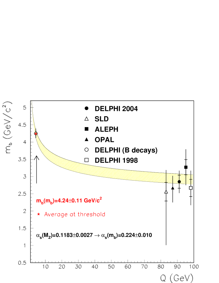
Figure 10: The evolution of $m_{b}(Q)$ as a function of the energy scale $Q$. The $m_{b}(M_{Z})$ measured by LEP and SLC are displayed together with their total and statistical errors. The shaded area corresponds to the band associated to $m_{b}(Q)$ when evolving the average value obtained at $m_{b}(m_{b})$ [13] up to the $M_{Z}$ scale using the QCD Renormalization Group Equations with $\alpha_{s}(M_{Z})=0.1183\pm 0.0027$. All these measurements are performed at the $M_{Z}$ energy scale but for display reasons they are plotted at different scales. The result obtained using Delphi data at low energy from semileptonic $B$ decays [34] is also shown.

Acknowledgements

We are greatly indebted to our technical collaborators, to the members of the CERN-SL Division for the excellent performance of the LEP collider, and to the funding agencies for their support in building and operating the DELPHI detector.
We acknowledge in particular the support of
Austrian Federal Ministry of Education, Science and Culture, GZ 616.364/2-III/2a/98,
FNRS–FWO, Flanders Institute to encourage scientific and technological research in the industry (IWT), Belgium,
FINEP, CNPq, CAPES, FUJB and FAPERJ, Brazil,
Czech Ministry of Industry and Trade, GA CR 202/99/1362,
Commission of the European Communities (DG XII),
Direction des Sciences de la Mati$\grave{\mbox{\rm e}}$re, CEA, France,
Bundesministerium f$\ddot{\mbox{\rm u}}$r Bildung, Wissenschaft, Forschung und Technologie, Germany,
General Secretariat for Research and Technology, Greece,
National Science Foundation (NWO) and Foundation for Research on Matter (FOM), The Netherlands,
Norwegian Research Council,
State Committee for Scientific Research, Poland, SPUB-M/CERN/PO3/DZ296/2000, SPUB-M/CERN/PO3/DZ297/2000, 2P03B 104 19 and 2P03B 69 23(2002-2004)
FCT - Fundação para a Ciência e Tecnologia, Portugal,
Vedecka grantova agentura MS SR, Slovakia, Nr. 95/5195/134,
Ministry of Science and Technology of the Republic of Slovenia,
CICYT, Spain, AEN99-0950 and AEN99-0761,
The Swedish Research Council,
Particle Physics and Astronomy Research Council, UK,
Department of Energy, USA, DE-FG02-01ER41155.
EEC RTN contract HPRN-CT-00292-2002.

We are specially grateful to A. Santamaría and G. Rodrigo for providing the NLO massive calculations that made this measurement possible. We are also indebted to T. Sjöstrand for his help in understanding how mass effects are implemented in Pythia. We would also like to thank G. Dissertori for the continuous feedback and J. Portoles and M. Eidemüller for their information about the $b$ pole mass.

References

[1]
M. Bilenky, G. Rodrigo and A. Santamaría, Nucl. Phys. B439 (1995) 505.
[2]
DELPHI Col., J. Abdallah et al., Eur. Phys. J. C32 (2004) 185
[3]
G.Rodrigo, A. Santamaría, M. Bilenky, Phys. Rev. Lett. 79 (1997)
193; G. Rodrigo, Nucl. Phys. B (Proc. Suppl.) 54 issue 3 (1997) 60.
[4]
W.Bernreuther, A. Brandenburg, P. Uwer, Phys. Rev. Lett. 79 (1997) 189.
[5]
P. Nason and C. Oleari, Phys. Lett. B407 (1997) 57.
[6]
M. Bilenky et al., Phys. Rev. D60 (1999) 114006.
[7]
DELPHI Coll., P.Abreu et al., Phys. Lett. B418 (1998) 430.
[8]
A. Brandenburg et al., Phys. Lett. B468 (1999) 168.
[9]
ALEPH Coll., R. Barate et al., Eur. Phys. J. C18 (2000) 1.
[10]
OPAL Coll., G. Abbiendi et al., Eur. Phys. J. C11 (1999) 643.
[11]
OPAL Coll., G. Abbiendi et al., Eur. Phys. J. C21 (2001) 411.
[12]
R. Tarrach, Nucl. Phys. B183 (1981) 384.
[13]
A.X. El-Khadra, M. Luke, Ann. Rev. Nucl. Part. Sci. 52 (2002) 201, [hep-ph/0208114].
[14]
A. H. Hoang, Frontier of Particle Physics / Handbook of QCD, Volume 4,
edited by M. Shifman (World Scientific, Singapore, 2001) 2215-2331.
[15]
V. M. Braun, Hadronic:0271-278 [hep-ph/9505317]
[16]
K.G. Chetyrkin and A. Kwiatkowski, Nucl. Phys. B461 (1996) 3.
[17]
K.G. Chetyrkin, B.A. Kniehl and M. Steinhauser, Phys. Rev. Lett. 79
(1997) 353.
[18]
K.G. Chetyrkin and M. Steinhauser, Phys. Lett. B408 (1997) 320.
[19]
Y.L. Dokshitzer et al., JHEP 9708 (1997) 001.
[20]
S. Catani et al., Phys. Lett. B269 (1991) 432;
N. Brown, W.J. Stirling, Z. Phys. C53 (1992) 629.
[21]
DELPHI Coll., P. Aarnio et al., Nucl. Instr. and Meth. A303 (1991) 233.
[22]
DELPHI Coll., P. Abreu et al., Nucl. Instr. and Meth. A378 (1996) 57.
[23]
T. Sjöstrand. Computer Phys. Commun. 82 (1994) 74.
[24]
G. Marchesini et al., Computer Phys. Commun. 67 (1992) 465.
[25]
DELPHI Coll., P. Abreu et al., Z. Phys. C73 (1996) 11.
[26]
T. Sjöstrand et al., Computer Phys. Commun. 135 (2001) 238; T. Sjöstrand, L. Lönnblad and S. Mrenna, PYTHIA 6.2 Physics and
Manual, [hep-ph/0108264].
[27]
G. Corcella et al., JHEP 0101 (2001) 010 [hep-ph/0011363];
[hep-ph/0201201].
[28]
C. Peterson et al., Phys. Rev. D27 (1983) 105.
[29]
M.G. Bowler, Z. Phys. C11 (1981) 169.
[30]
A. De Rújula, H. Georgi, S.L. Glashow, Phys. Rev. D12 (1975) 147.