Shortest movie: Bose-Einstein Correlation functions in $\mathrm{e}^{+}\mathrm{e}^{-}$ annihilations

Abstract

Bose-Einstein correlations of identical charged-pion pairs produced in hadronic Z decays are analyzed in terms of various parametrizations. A good description is achieved using Lévy stable distributions. The source function is reconstructed with the help of the $\tau$-model.

1 Introduction

In particle and nuclear physics intensity interferometry provides a direct experimental method for the determination of sizes, shapes and lifetimes of particle-emitting sources (for recent reviews see Wolfram ; Tamas1 ). In particular, boson interferometry provides a powerful tool for the investigation of the space-time structure of particle production processes, since Bose-Einstein correlations (BEC) of two identical bosons reflect both geometrical and dynamical properties of the particle radiating source.

In $\mathrm{e}^{+}\mathrm{e}^{-}$ annihilation BEC are maximal if the invariant momentum difference is small, even when one of the relative momentum components is large, as was seen by TASSO tasso and which we have confirmed. For a hydrodynamical type of source, on the contrary, BEC decrease when any of the relative momentum components is large Tamas1 ; Tamas2 .

Here we investigate various parametrizations and find that a good description of the Bose-Einstein correlation function can be achieved using Lévy stable distributions as the source function. Within the framework of models assuming strongly correlated coordinate and momentum space, we then reconstruct the complete space-time picture of the particle emitting source in hadronic Z decay.

For our analysis we use a sample of about 500 thousand two-jet events, selected by the Durham algorithm durham with $y_{\mathrm{cut}}=0.006$, from e⁺e^-annihilation data collected by L3 at a center-of-mass energy of 91.2 GeV.

2 Parametrizations of BEC

The two-particle correlation function is defined as:

$$R_{2}(p_{1},p_{2})=\frac{\rho_{2}(p_{1},p_{2})}{\rho_{1}(p_{1})\rho_{1}(p_{2})},$$ (1)

where $\rho_{2}(p_{1},p_{2})$ is the two-particle invariant momentum distribution, $\rho_{1}(p_{i})$ the single-particle invariant momentum distributions and $p_{i}$ the four-momentum of particle $i$. Since we are only interested in BEC, the product of single particles densities is replaced by the so-called reference sample, $\rho_{0}(p_{1},p_{2})$, the two-particle density that would occur in the absence of Bose-Einstein interference. Here we use mixed events as a reference sample.

After some assumptions Wolfram ; Tamas1 , this two-particle correlation function is related to the Fourier transformed source distribution. In this case

$$R_{2}(p_{1},p_{2})=1+|\tilde{f}(Q)|^{2},$$ (2)

where $f(x)$ is the density distribution of the source, $Q$ is the invariant four-momentum difference, $Q=-(p_{1}-p_{2})^{2}$ and $\tilde{f}(Q)$ is the Fourier transform of $f(x)$.

2.1 Gaussian distributed source

The simplest assumption is that the source has a symmetric Gaussian distribution, in which case $\tilde{f}(Q)=\exp\left(i\mu Q-\frac{(RQ)^{2}}{2}\right)$ and

$$R_{2}(Q)=\gamma\left[1+\lambda\exp\left(-(RQ)^{2}\right)\right]\left(1+\delta Q\right),$$ (3)

where the parameter $\gamma$ is a constant of normalization, $\lambda$ an incoherence factor, which measures the strength of the correlation, and $\left(1+\delta Q\right)$ is introduced to parametrize possible long-range correlations not adequately accounted for in the reference sample.

A fit of Eq.(3) to the data results in an unacceptably low confidence level from which we conclude that the shape of the source deviates from a Gaussian. The fit is particularly bad at low $Q$ values.

2.2 Lévy distributed source

Adopting Nolan’s $S(\alpha,\beta=0,\gamma,\delta;1)$ convention Nolan for the symmetric Lévy stable distribution with rescaling of the scale parameter $\gamma$ to $R$ and the location parameter $\delta$ to $x_{0}$, the Fourier transform (characteristic function) $\tilde{f}(Q)$ has the following general form:

$$\tilde{f}(Q)=\exp(iQx_{0}-|RQ|^{\alpha}).$$ (4)

The index of stability, $\alpha$, satisfies the inequality $0<\alpha\leq 2$. The case $\alpha=2$ corresponds to a Gaussian source distribution. For more details see Nolan .

Then $R_{2}$ has the following, relatively simple form Tamas3 :

$$R_{2}(Q)=\gamma\left[1+\lambda\exp\left(-(RQ)^{\alpha}\right)\right](1+\delta Q).$$ (5)

After fitting Eq.(5) to the data it is clear that the correlation function is far from Gaussian: $\alpha\approx 1.3$. The confidence level, although improved compared to the fit of Eq.(3), is still unacceptably low.

Since there is no particle production before the onset of the collision, a more appropriate form of the source distribution for the time component is the asymmetric stable distribution. In this case, one obtains the following result for the correlation function Tamasbesz :

$$R_{2}(Q)=\gamma\left[1+\lambda\cos\left[(R_{\mathrm{a}}Q)^{\alpha}\right]\exp\left(-(RQ)^{\alpha}\right)\right](1+\delta Q),$$ (6)

where $R_{\mathrm{a}}$ is an additional parameter, a measure of the onset of particle production Nolan ; Tamas3 .

The fit of Eq.(6) to the data, shown in Figure 1, is statistically acceptable. The data are well described by the fit. Note that for $Q$ between 0.5 $\mathrm{GeV}$ and 1.5 $\mathrm{GeV}$ the data points go below the dashed line, which stands for the long-range correlations extrapolated to lower $Q$ values. These data points indicate an anti-correlation in the $Q\approx 1$ GeV region. This property of the data is well reproduced by the fitted curve, which also goes below unity as a result of the cosine term in Eq.(6), which comes from the asymmetric Lévy assumption. The fitted value of $\alpha$ is $0.82\pm 0.03$.

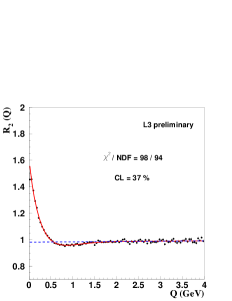
Figure 1: The Bose-Einstein correlation function $R_{2}$. The curve corresponds to the fit of Eq.(6).

3 The $\tau$-model

A model of strongly correlated phase-space was developed Tamas4 to explain the experimentally found invariant relative momentum $Q$ dependence of Bose-Einstein correlations in $\mathrm{e}^{+}\mathrm{e}^{-}$ reactions. This model also predicts a specific transverse mass dependence of $R_{2}$, that we subject to an experimental test here.

In this model, it is assumed that the average production point $\overline{x}^{\mu}$ of particles with a given momentum $k^{\mu}$ is given by

$$\overline{x}^{\mu}(k^{\mu})=dk^{\mu}.$$ (7)

In the case of two-jet events, $d=\frac{\tau}{m_{\mathrm{T}}}$, where $\tau=\sqrt{t^{2}-k_{z}^{2}}$ is the longitudinal proper-time and $m_{\mathrm{T}}=\sqrt{m^{2}+p_{\mathrm{T}}^{2}}$ is the transverse mass. The second assumption is that the distribution of $x^{\mu}(k^{\mu})$ about its average, $\delta_{\Delta}(x^{\mu}(k^{\mu})-\overline{x}^{\mu}(k^{\mu}))$, is narrower than the proper-time distribution. Then the emission function of the $\tau$-model is

$$S(x,k)=\int_{0}^{\infty}\mathrm{d}\tau H(\tau)\delta_{\Delta}(x-dk)N_{1}(k),$$ (8)

where $H(\tau)$ is the longitudinal proper-time distribution, the factor $\delta_{\Delta}(x-dk)$ describes the strength of the correlations between coordinate space and momentum space variables and $N_{1}(k)$ is the experimentaly measurable single-particle spectrum.

In the plane-wave approximation the Yano-Koonin formula Yano gives the following two-pion multiplicity distribution:

$$\rho_{2}(k_{1},k_{2})=\int\mathrm{d}^{4}x_{1}\mathrm{d}^{4}x_{2}S(x_{1},k_{1})S(x_{2},k_{2})\left(1+\cos\left[(k_{1}-k_{2})(x_{1}-x_{2})\right]\right).$$ (9)

Approximating the $\delta_{\Delta}$ function by a Dirac delta function, the argument of the cosine becomes

$$(k_{1}-k_{2})(\bar{x}_{1}-\bar{x}_{2})=-0.5(d_{1}+d_{2})Q^{2}.$$ (10)

Then the two-particle Bose-Einstein correlation function is approximated by

$$R_{2}(k_{1},k_{2})=1+\lambda\mathrm{Re}\widetilde{H}^{2}\left(\frac{Q^{2}}{2\overline{m}_{\mathrm{T}}}\right),$$ (11)

where $\widetilde{H}(\omega)=\int\mathrm{d}\tau H(\tau)\exp(i\omega\tau)$ is the Fourier transform of $H(\tau)$. Thus an invariant relative momentum dependent BEC appears.

Guided by the result of the previous section, we use an asymmetric Lévy distribution for the longitudinal proper-time density. Thus the corresponding BEC function has an analytic, although somewhat complicted form Tamas3 ; Tamasbesz :

$$R_{2}(Q^{2},\overline{m}_{\mathrm{T}})=\gamma\Bigg{[}1+\lambda\cos\left(\frac{\tau_{0}Q^{2}}{\overline{m}_{\mathrm{T}}}+A\left(\frac{\Delta\tau Q^{2}}{\overline{m}_{\mathrm{T}}}\right)^{\frac{\alpha}{2}}\right)\exp\left(-\left(\frac{\Delta\tau Q^{2}}{\overline{m}_{\mathrm{T}}}\right)^{\frac{\alpha}{2}}\right)\Bigg{]}B$$ (12)

where the parameter $\tau_{0}$ is the proper-time of the onset of particle production, $\Delta\tau$ is a measure of the width of the proper-time distribution, $A=\tan\left(\frac{\alpha\pi}{4}\right)$ and $B=(1+\delta Q)$

After fitting for various $\overline{m}_{\mathrm{T}}$ interval we find that the quality of the fits is statistically acceptable and the fitted values of the model parameters are stable and within errors the same in all investigated $m_{\mathrm{T}}$ interval. The $\tau$-model with a one-sided Levy proper-time distribution describes the data with parameters $\tau_{0}=0$ fm, $\alpha\approx 0.80\pm 0.05$ and $\Delta\tau\approx 2.0\pm 0.6$ fm.

4 Reconstruction of the emission function

In order to reconstruct the space-time picture of the emitting process we assume that the emission function can be factorized in the following way:

$$S(r,z,t)=I(r)G(\eta)H(\tau),$$ (13)

where $I(r)$ is the single-particle transverse distribution, $G(\eta)$ is the space-time rapidity distribution of particle production, which approximately coincides with the single-particle rapidity distribution, and $H(\tau)$ is the observed proper-time distribution.

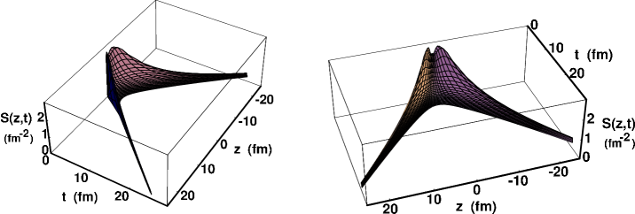
Figure 2: Two views of the longitudinal part of the source function normalized to the average number of pions per event.

With these assumptions one can reconstruct the longitudinal part of the emission function integrated over the transverse distribution. It is plotted as a function of $t$ and $z$ in Figure 2. It exhibits the typical boomerang shape with a maximum at low $t$ and $z$ but with tails reaching out to very large $t$ and $z$ values, a feature already observed for hadron-hadron NA22 and heavy ion collisionsSter .

The transverse profile, which follows from Eq. (8), has the following form:

$$\frac{\mathrm{d}^{4}n}{\mathrm{d}\tau\mathrm{d}^{3}r}=\frac{m_{\mathrm{T}}^{3}}{\tau^{3}}H(\tau)N_{1}\left(k=\frac{m_{\mathrm{T}}r}{\tau}\right).$$ (14)

This equation describes the particle production in coordinate space as a function of the proper-time $\tau$. It describes the expansion of the source as the proper-time increases. The particle production probability is proportional to the proper-time distribution $H(\tau)$. Figure 3 shows the transverse part of the emission function for various proper-times. Particle production starts immediately, increases rapidly and decreases slowly. A ring-like structure, similar to the expanding, ring-like wave created by a pebble in a pond, is reconstructed from L3 data, as shown in Fig. 3. An animated gif file that shows this effect is available from Movie .

Figure 3: The source function normalized to the average number of pions per event for various proper-times.

References

- (1) W. Kittel, Acta Phys. Pol. B32 (2001) 3927.
- (2) T. Csörgő, Heavy Ion Physics 15, (2002) 1.
- (3) M. Althoff et al. (TASSO Collab.), Z. Phys C30 (1986) 355.
- (4) T. Csörgő and B. Lörstadt, Phys. Rev. C54 (1996) 1390.
- (5) S. Cantani et al., Phys. Lett. B279 (1991) 432.
- (6) J. P. Nolan, Stable distributions: Models for Heavy Tailed Data http://academic2american.edu/ jpnolan/stable/CHAP1.PDF
- (7) T. Csörgő, S. Hegyi, W. A. Zajc Eur. Phys. J. C36 (2004) 67. hep-ph/0301164
- (8) T. Csörgő, private communication
- (9) T. Csörgő and J. Zimányi, Nucl. Phys. A517 (1990) 588.
- (10) F. B. Yano amd S. E. Koonin, Phys. Lett. textbfB78 (1978) 556.
- (11) N. M. Agababyan at al. (NA22 Collab.), Phys. Lett. B422 (1998) 359.
- (12) A. Ster, T. Csörgő and B. Lörstad, Nucl. Phys A661 (1999) 419.
- (13) www.hef.kun.nl/ novakt/movie/movie.gif