Transverse-longitudinal HBT correlations
in $\mathbf{p\bar{p}}$ collisions at $\mathbf{\sqrt{s}=630}$ GeV

Abstract

Correlations of like-sign pion pairs emerging from proton-antiproton collisions are analysed in the two-dimensional $(q_{L},q_{T})$ decomposition of the three-momentum difference ${\mathbf{q}}$. While the data cannot be adequately represented by gaussian, exponential, power-law or Edgeworth parametrisations, more elaborate ones such as Lévy and an exponential with a cross term do better. A two-scale model using a hard cut to separate small and large scales may indicate a core that is more prolate than the halo. Consideration not only of the interference peak at small $(q_{L},q_{T})$, but also of the shape of the correlation distribution at intermediate momentum differences is crucial to understanding the data.

PACS: 13.85.Hd, 13.87.Fh, 13.85.-t, 25.75.Gz

and

1 Introduction

The measurement of correlations between identical final-state particles, also commonly termed “Bose-Einstein correlations” or “HBT effect” after the fathers of intensity interferometry in astronomy, has become a valuable tool in the quest to understand the spacetime structure of high-energy collision processes [1, 2]. The recently-coined term of femtoscopy highlights the possibilities of unraveling the interplay of kinematics and dynamics at the femtometer level based on the symmetrisation of identical bosons.

The current concentrated effort at RHIC to quantify and understand ultrarelativistic nuclear collisions [3] relies extensively on comparisons with baseline scenarios constructed from the corresponding “trivial” hadron-hadron sample. In this context, the UA1 experiment continues to be relevant and interesting, even though data-taking at the CERN SPS has long ceased. Current experimental energies of $200$ AGeV at RHIC are still below those available to UA1 by a factor three, so that our results may also provide a window on possible energy dependencies of current investigations.

One of the relevant theoretical frameworks is constructed in terms of a three-dimensional decomposition of the pair momentum difference, ${\mathbf{q}}={\mathbf{p}}_{1}-{\mathbf{p}}_{2}$ along the collision axis, the pair transverse momentum and the “side” direction orthogonal to both [4]. In this letter, we provide results on HBT analysis in terms of the simpler two-dimensional decomposition, defining in the usual way $q_{L}=|\mathbf{q}_{L}|=|(\mathbf{q}\mathbf{\cdot}\hat{\mathbf{z}})\,\hat{\mathbf{z}}|$, with $\hat{\mathbf{z}}$ the beam direction, and $q_{T}=|\mathbf{q}-\mathbf{q}_{L}|$. We analyse correlations between like-sign (LS) pion pairs in terms of the normalised second moment,

$$R_{2}(q_{L},q_{T})=\frac{\rho_{2}^{\rm sib}(q_{L},q_{T})}{\rho_{2}^{\rm ref}(q_{L},q_{T})}\,,$$ (1)

where $\rho_{2}^{\rm sib}(q_{L},q_{T})$ counts “sibling” LS pairs from the same event, while $\rho_{2}^{\rm ref}(q_{L},q_{T})$ counts “reference” pairs made up through event mixing.

2 Data sample, cuts and corrections

Like-sign pion pairs from approximately 2.45 million minimum-bias events [5] measured by the UA1 central detector in 1985 and 1987 were analysed. We applied the same single-track cuts used previously [6], including $p_{\bot}\geq 0.15$ GeV $|\eta|\leq 3$ and $45^{\circ}\leq|\phi|\leq 135^{\circ}$. Good measurement quality and fitted track length $\ell>30$ cm were required. The sample contains mainly pions with an estimated 15% contamination of charged kaons and protons [7].

As in previous work [8, 6], an angle cut was applied due to limited angular resolution in the central detector [9], and pairs were required to have minimum four-momentum difference $Q^{2}=\sqrt{-(p_{1}-p_{2})^{2}}>0.0003$ GeV².

Spurious “split–track” pairs strongly influence pair counts at small relative momenta. Besides eliminating these pairs with the same algorithm used in previous analyses, we now also correct for the fact that this necessarily eliminates some physical like-sign track pairs. We determine correction factors for each $(q_{L},q_{T})$ bin measured in the detector rest system and charged-multiplicity subsample (see below) by passing unlike-sign pairs through the same split-track algorithm. These correction factors are substantial at small $(q_{L},q_{T})$, reaching 1.9 for low-multiplicity subsamples. Errors shown and quoted take into account the additional uncertainty introduced by the correction.

We corrected for Coulomb repulsion by parametrising the Bowler Coulomb correction in the invariant momentum difference [10] with an exponentially damped Gamov factor $G(Q)$ [11], $F_{\rm coul}(Q)=1+\left[G(Q)-1\right]\,\exp(-Q/Q_{\rm eff})$, with a best-fit value $Q_{\rm eff}=0.173\pm 0.001$ GeV.

Correlations from subsamples of fixed $N$, the observed charged multiplicity in the whole azimuth, were summed separately in the numerator and denominator

$$R_{2}(\mathbf{q})=\frac{\sum_{N}P_{N}\,\rho_{2}({\mathbf{q}}\,|\,N)}{\sum_{N}P_{N}\,(1-N^{-1})\,\rho_{1}{\otimes}\rho_{1}({\mathbf{q}}\,|\,N)}\,.$$ (2)

The sum $\sum_{N}P_{N}$ was implemented in terms of ten subsamples defined by multiplicity $N$. The reference for each $N$-subsample, $\rho_{1}{\otimes}\rho_{1}({\mathbf{q}}\,|\,N)$, was constructed by creating for each sibling event a set of fake events with the same multiplicity, using tracks randomly selected from the corresponding subsample track pool. The factor $(1-N^{-1})=N(N{-}1)/N^{2}$ arises because the uncorrelated reference for fixed-$N$ subsamples is not the poisson but the multinomial distribution [12]. All HBT quantities are measured in the longitudinal co-moving system (LCMS) of the pion pair.

3 Parametrisations

We use the generic parametrisation $R_{2}(q_{L},q_{T})=\gamma\left[1+\lambda\left|S\right|^{2}\right],$ where the multiplicative parameter $\gamma$ corrects for any remaining effect of the overall multiplicity distribution, $\lambda$ is the “chaoticity parameter” and $S(q_{L},q_{T})$ corresponds to the Fourier-transformed source function. For $|S|^{2}$, we implemented the simple gaussian, the gaussian with cross-term [13], the simple exponential, and the exponential with cross-term parametrisations,

$$|S|^{2} = \exp(-R_{L}^{2}q_{L}^{2}-R_{T}^{2}q_{T}^{2})\,,$$ (3)

$$|S|^{2} = \exp(-R_{L}^{2}q_{L}^{2}-R_{T}^{2}q_{T}^{2}-2R_{LT}^{2}q_{L}q_{T})\,,$$ (4)

$$|S|^{2} = \exp(-R_{L}q_{L}-R_{T}q_{T})\,,$$ (5)

$$|S|^{2} = \exp(-R_{L}q_{L}-R_{T}q_{T}-2R_{LT}\sqrt{q_{L}\,q_{T}})\,,$$ (6)

as well as a power-law parametrisation,

$$R_{2}=\gamma\left[1+(R_{L}q_{L})^{-\alpha_{L}}\,(R_{T}q_{T})^{-\alpha_{T}}\right]\,.$$ (7)

Apart from the above parametrisations, nongaussian distributions can also be approached through Edgeworth expansions [14, 15],

$$\left|S\right|^{2}=\exp(-R_{L}^{2}q_{L}^{2}-R_{T}^{2}q_{T}^{2})\prod_{d=L,T}\left[1+\kappa_{4,d}\;H_{4}(\sqrt{2}\,R_{d}\,q_{d})/24\right],$$ (8)

or through Lévy distributions [16],

$$\left|S\right|^{2} = \exp(-R_{L}^{2}q_{L}^{2}-R_{T}^{2}q_{T}^{2})^{\alpha/2}\,,$$ (9)

$$\left|S\right|^{2} = \exp(-R_{L}^{2}q_{L}^{2}-R_{T}^{2}q_{T}^{2}-2R_{LT}^{2}q_{L}q_{T})^{\alpha/2}.$$ (10)

All fits with the above parametrisations were performed over the whole region $0\leq q_{L},q_{T}\leq 0.5\,$GeV but omitting the bin $(q_{L},q_{T})<(0.02,0.02)\,$GeV which suffers from multiple large corrections and detector effects. Note that values for $R_{L}$ and $R_{T}$ cannot be compared between different parametrisations; note also that these parameters play the traditional role of “radius” of a distribution, and can be related to various source parameters [17], only for the gaussian cases (3)–(4).

4 Analysis and Results

4.1 The region of small $(q_{L},q_{T})$

Fig. 1 shows slices of $R_{2}(q_{L},q_{T})$ for fixed $q_{T}$ bins in the upper and fixed $q_{L}$ bins in the lower panels, together with the global fits based on Eqs. (3)–(10). The Gauss, Gauss-with-cross-term, and Edgeworth fits are practically indistinguishable, as $R_{LT}$ in (4) is compatible with zero and cumulants $\kappa_{4,L}$ and $\kappa_{4,T}$ in (8) do not improve the fit. All three are equally bad, with $\chi^{2}/{\rm NDF}\sim 3.3$. The simple exponential (5) (not shown) is even worse at 4.0. The cross-term exponential, however, has $\chi^{2}/\mbox{NDF}=1.7$. The power law (7) is a disaster at $\chi^{2}/\mbox{NDF}=16$.

Both Lévy-based parametrisations (9)–(10) fare better in reproducing the strong peak observed in the data, with $\chi^{2}/\mbox{NDF}=1.45$ and $1.13$ respectively. However, the fit parameters $\lambda$, $R_{L}$, $R_{T}$, $R_{LT}$ and $\alpha$ are strongly correlated so that there is no unique minimum and therefore no unique set of best-fit parameter values. All that can be said with some confidence is that $\alpha$ is around 0.20–0.23, that $R_{L}$ and $R_{T}$ are of order $10^{3}\,$fm with $R_{L}/R_{T}$ = 1.6, and that $R_{LT}^{2}$ is negative; we will return to this below. Omitting a second small-$(q_{L},q_{T})$ bin from the Lévy fits renders them even more unstable. This is hardly surprising, as the above parameters collectively depend strongly on the exact shape of the peak in the very small $(q_{L},q_{T})$ region, the very region that experimental measurement struggles to resolve.

4.2 Observations at intermediate $(q_{L},q_{T})$

Fig. 1, revealing as it is, tells only part of the story as it focuses exclusively on the peak at small $|{\mathbf{q}}|$. Intermediate scales, it turns out, are very important.

In Fig. 2, the same data and some of the fits are shown as colour maps over the full set of bins, but with the peaks in the lower left corners truncated at $R_{2}=1.9$ in order to highlight structure at intermediate $(q_{L},q_{T})$ scales. Panel (b) shows that the simple exponential (5) cannot possibly describe the data as its shape at intermediate scales is linear, while the data in (a) is elliptic. The Lévy without cross term (9), Panel (e), matches the shape better. Panels (c) and (f), representing the exponential and Lévy with cross terms included, most accurately reflect the data structure. The gaussian forms (4) and (8) have a shape similar to that in (e). From Panel (d), it is immediately apparent that the spectacular failure of the power law (7) stems from its hyperbolic shape. A “sum power law” $R_{2}=\gamma\left[1+(R_{L}\,q_{L})^{-\alpha_{L}}+(R_{T}\,q_{T})^{-\alpha_{T}}\right]$ fares even worse.

Figure 2 also makes clear that the source — whatever its exact shape — is prolate, i.e. $R_{L}>R_{T}$ must hold for all parametrisations.

4.3 A two-scale approach.

The strong peak seen in the data and the comparatively large values for $\chi^{2}$ for the above parametrisations suggests that there may be two scales in the system. Borrowing the terms “core” and “halo” from the literature [18], one may try a simultaneous fit to a double-gaussian parametrisation [19, 20],

$$R_{2}(q_{L},q_{T})=\gamma\left[1+\lambda_{C}\exp(-R_{LC}^{2}q_{L}^{2}-R_{TC}^{2}q_{T}^{2})+\lambda_{H}\exp(-R_{LH}^{2}q_{L}^{2}-R_{TH}^{2}q_{T}^{2})\right].$$ (11)

However, again there are too many parameters, so that there is no unique set of best-fit values. For this reason, we try a “two-scale” procedure, starting from the assumption that the two scales implicit in (11) can be separated by a hard cut in the data. First, we fit to the core gaussian only bins with momentum differences larger than a cutoff ($q_{L}>q_{\rm cut}$ or $q_{T}>q_{\rm cut}$), thereby fixing $\gamma$, $\lambda_{C},R_{LC}$ and $R_{TC}$. This core gaussian is then subtracted from all data, after which the remaining halo “data” with $(q_{L},q_{T})\leq(q_{\rm cut},q_{\rm cut})$ is fit with the halo gaussian $\gamma\,\lambda_{H}\exp(-R_{LH}^{2}q_{L}^{2}-R_{TH}^{2}q_{T}^{2})$ for fixed $\gamma$. Finally, the resulting core and halo fits are combined.

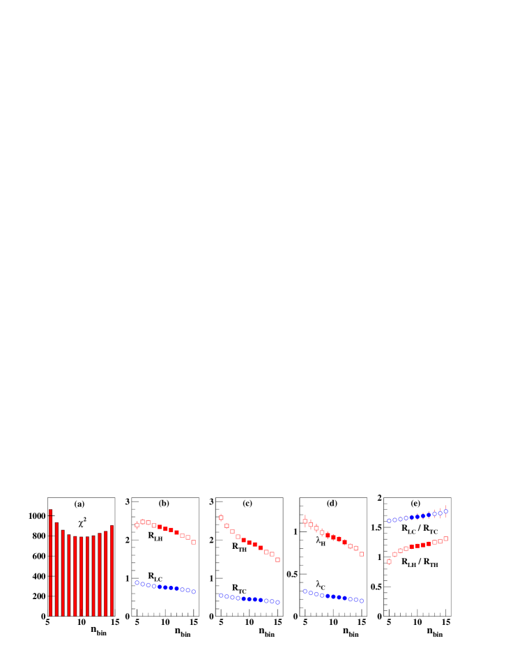
Figure 3: Dependence on $q_{\rm cut}$. (a) Combined $\chi^{2}$ for core and halo fits as a function of $q_{\rm cut}=(0.02\,n_{\rm bin})\,$GeV. The four lowest $\chi^{2}$ values correspond to $q_{\rm cut}=0.18{-}0.24\,$GeV and $\chi^{2}/\mathrm{NDF}=1.28$. (b)–(e): Dependence of parameter values on $q_{\rm cut}$. Filled points correspond to the four smallest $\chi^{2}$ in (a).

This procedure must be tested for consistency. As shown in Fig. 3(a), the joint $\chi^{2}$ for both fits as a function of $q_{\rm cut}=0.02\,n_{\rm bin}$ is found to have a minimum in the interval $q_{\rm cut}=$ 180–240 MeV. The joint best $\chi^{2}/{\rm NDF}=1.28$ for the two-scale model is comparable to those for the Lévy fits and fit values are stable, so that numbers can be quoted. The $R_{L}$, $R_{T}$, $\lambda$ and $R_{L}/R_{T}$ values corresponding to the four smallest $\chi^{2}$ values are shown as filled points in Fig. 3(b)–(e). Averaging these numbers, we estimate $R_{LC}=0.75\pm 0.02$ fm, $R_{TC}=0.45\pm 0.02$ fm, $R_{LH}=2.26\pm 0.07$ fm, and $R_{TH}=1.89\pm 0.10$ fm, signalling a prolate core and a somewhat more spherical halo. We note that best-fit chaoticities $\lambda_{C}=0.23\pm 0.01$ and $\lambda_{H}=0.92\pm 0.04$ are below the theoretical limit of 1, while the large intercept seen in the data itself ($R_{2}(0,0)>3.7$) and corresponding single-component chaoticities ($\lambda\sim 2.7$) violate this limit.

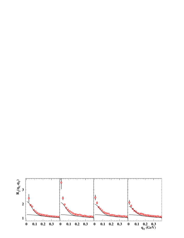
Figure 4: $R_{2}(q_{L},q_{T})$ and fit to core (lower lines) and combined core-halo (upper lines), shown in the upper panels for slices with fixed $q_{T}=$ 0.00–0.02, 0.02–0.04, 0.04–0.06 and 0.06–0.08 GeV and in the lower panels for corresponding fixed-$q_{L}$ slices.

In Fig. 4, the upper lines show the combined two-scale best fit for $q_{T}$ and $q_{L}$ slices, with the lower lines corresponding to the core. While there is substantial improvement over simple parametrisations especially at intermediate scales, data points in the peak remain consistently above even this fit.

It must be emphasised that this two-scale procedure can work only if its assumptions are confirmed a posteriori. First, the resulting halo gaussian must, and does, become negligible at scales larger than $q_{\rm cut}$ for the ansatz to be valid. Also, the clear separation between the sizes of the core and halo radii seen in Fig. 3 do not contradict the assumption of the presence of two scales. For this data set, the two-scale model is consistent.

4.4 Systematic errors and uncorrected data

The above results have shown that the data appears to have a strong peak below 0.10 GeV which significantly exceeds all parametrisations tried. While it is tempting to conclude that the peak represents some physical effect, other possibilities must be checked. We hence conducted a survey of effects that various cuts and corrections have on $R_{2}$. We find that the angle cut and $Q^{2}$ cut and the restriction in azimuth have very little effect on the normalised moment and that any systematic error due to these is of the order of a few percent.

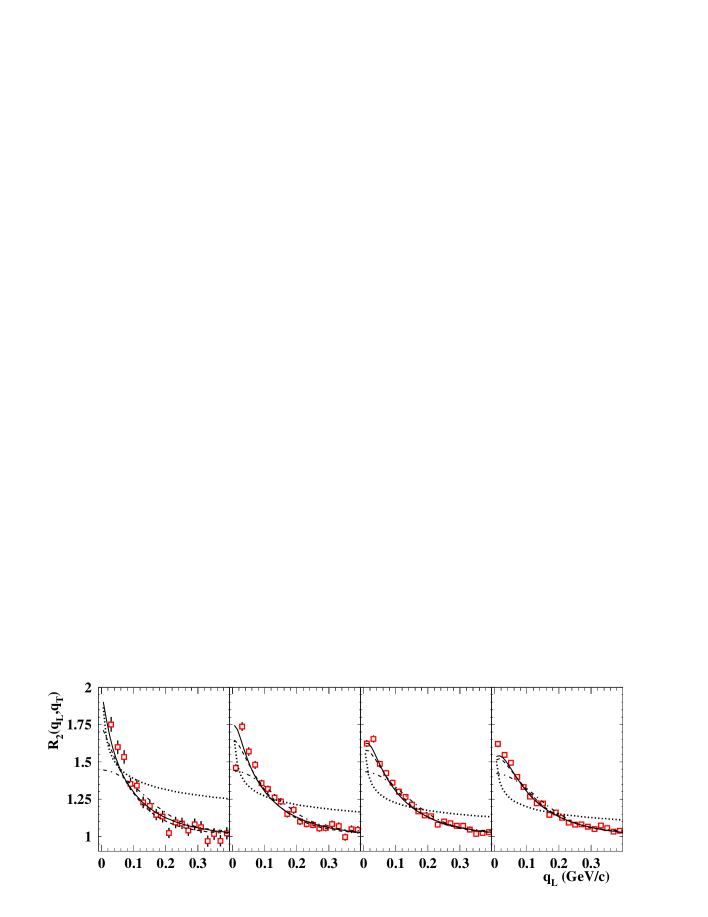
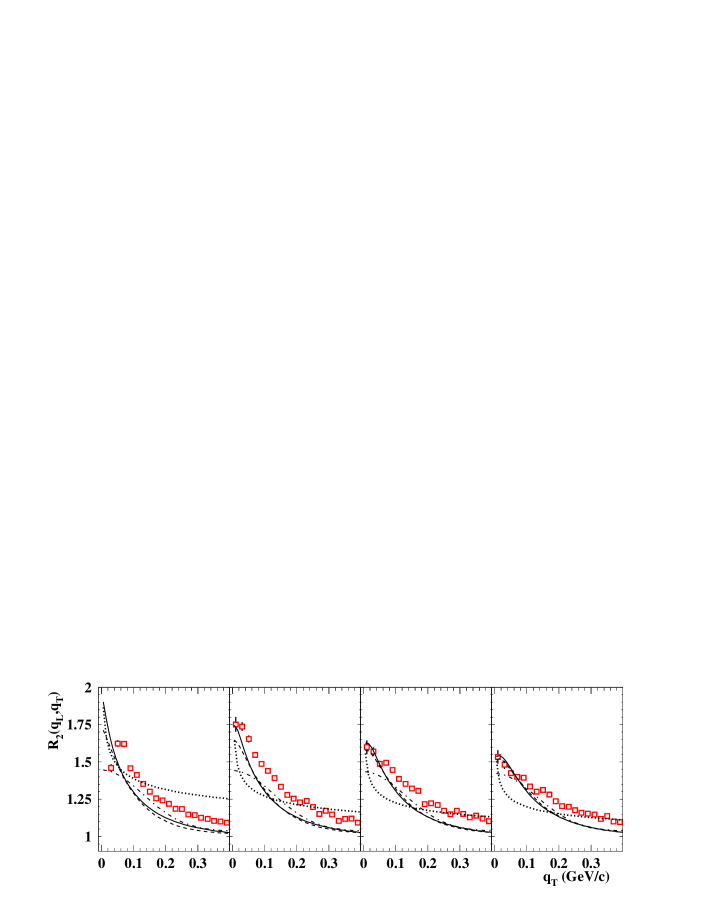
Figure 5: Same as Fig. 1 but for uncorrected data and including power law (dotted line). Note the different vertical scale.

However, the correction for the unwarranted removal of real LS track pairs by the split-track algorithm is large, and it is concentrated in precisely the region where the large peak occurs. Naturally, one must ask whether the entire excess of the data over various parametrisations reflects nothing but the correction itself. Taking the extreme approach of leaving the correction out altogether, we have repeated the entire analysis for the uncorrected data, which is shown in Fig. 5 together with the same set of parametrisations used in Fig. 1 plus the power law (7).

It is immediately apparent that the uncorrected data peak cannot be described by gaussian parametrisations either ($\chi^{2}/{\rm NDF}\sim 3.5$). With regard to shape (not shown), the general elliptic and prolate form of the data remains unchanged. The various parametrisations follow the pattern set by Fig. 2: again, the simple exponential and power law fail because they do not reproduce the shape of the data; again, the Lévy and exponential with cross term work better, with the latter faring best. While fit parameter values (e.g. of the Lévy-fits with $R_{L}\sim$ 2.5–2.9 fm, $R_{T}\sim$ 1.6–1.8 fm and $\alpha\sim 0.7$) differ from those of the corrected data, the conclusions regarding the success of particular parametrisations are hence independent of the split-track correction.

5 Discussion and Conclusions

The present results on HBT correlations extend UA1 observations to multidimensional correlations for the first time, which, at 630 GeV, represent the highest CMS energy at which this has been done. Two issues stand out: the strength of the peak at small momentum differences, and the importance of shape at intermediate scales.

With a strong peak at small $q_{L},q_{T}\leq 0.1\,$GeV, our high-statistic data, with and without corrections, rules out parametrisations based on single gaussians and their derivatives. While some other parametrisations are strongly peaked, none of those tried, not even the Lévy and two-scale cases, reproduces the peak data convincingly. This may hint that “something else is going on”, be it the influence of jets, resonances, clustering effects or some other unknown factor. The two-scale results may hint that the “halo” could be due to short-lived resonances such as the $\rho$.

We stress that it is unlikely that the strong peak seen in our data at small momentum differences is due to bias. First, the peak persists even without the Coulomb or split-track corrections. Second, the nongaussian behaviour seen in this paper is in line with UA1 one-dimensional correlation structures seen earlier in the form of nonzero higher-order cumulants [7, 21] and in the power law in $Q^{2}$ [8, 22], even though the data had not been corrected in the way it has been here. Third, the presence of unidentified kaons and protons in the sample imply that the real peak should exceed the one shown here, so that the present results are conservative. It should be noted that a number of other hadronic experiments [23, 24, 25] have also seen significant deviations from gaussian behaviour at small $|\mathbf{q}|$.

Besides the structure of the peak seen at small scales, the shape of the distribution at intermediate scales is seen to provide valuable additional information. Fig. 2 shows that the data has without doubt an elliptic and prolate shape, the latter in the sense that the distribution in momentum space is narrower in the longitudinal than in the transverse direction. This is confirmed also within the two-scale method and for the uncorrected data. Significantly, these conclusions are independent of the various parametrisations and corrections.

Second, plots of shape (whether in colour or as contour lines) help to constrain possible parametrisations: whereas in the one-dimensional analysis of UA1 data [8], the exponential and power-law parametrisations were found to be superior to the gaussian, their extension to two dimensions fails badly because their contour lines are straight lines or even hyperbolic.

Considering shape in terms of different parametrisations is complementary to decompositions into cartesian and spherical harmonics [26, 27], which can be expected to work best for near-gaussian data. We note, however, that the interrelationship between shape and algebraic form of a parametrisation is less than obvious: elliptic shape is exhibited not only by bilinear forms such as Eqs. (3)–(4) and (9)–(10) but also, surprisingly, by the exponential-with-cross-term, whose success depends strongly on the sign of the cross term. For both exponential (6) and Lévy with cross-term (10), our data clearly prefers negative values for the cross term ($R_{LT}$ and $R_{LT}^{2}$ respectively); positive values result in more hyperbolic shapes, in conflict with the data.

Their fit instability nonwithstanding, the Lévy parametrisations, which have the right shape and an acceptable peak, appear promising. Taking these at face value would imply that the corresponding source falls off with a power-law tail at large distances [16, 28, 29].

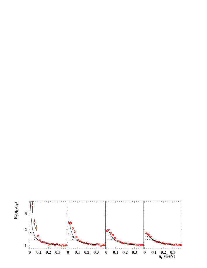
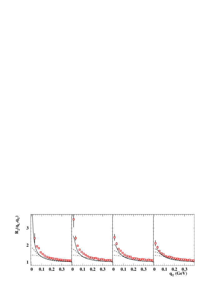
Figure 1: Upper panels: $R_{2}(q_{L},q_{T})$ data and best fits, shown left to right for slices with fixed $q_{T}=$ 0.00–0.02, 0.02–0.04, 0.04–0.06 and 0.06–0.08 GeV bins. Solid lines: Lévy fit (10); dashed: exponential with cross term; dash-dotted: Gauss/Edgeworth. Lower panels: $R_{2}(q_{L},q_{T})$ and the same fits for corresponding fixed-$q_{L}$ slices. Throughout this letter, fits are performed over all 624 data points, not just the data points, slices and intervals shown in the figures.

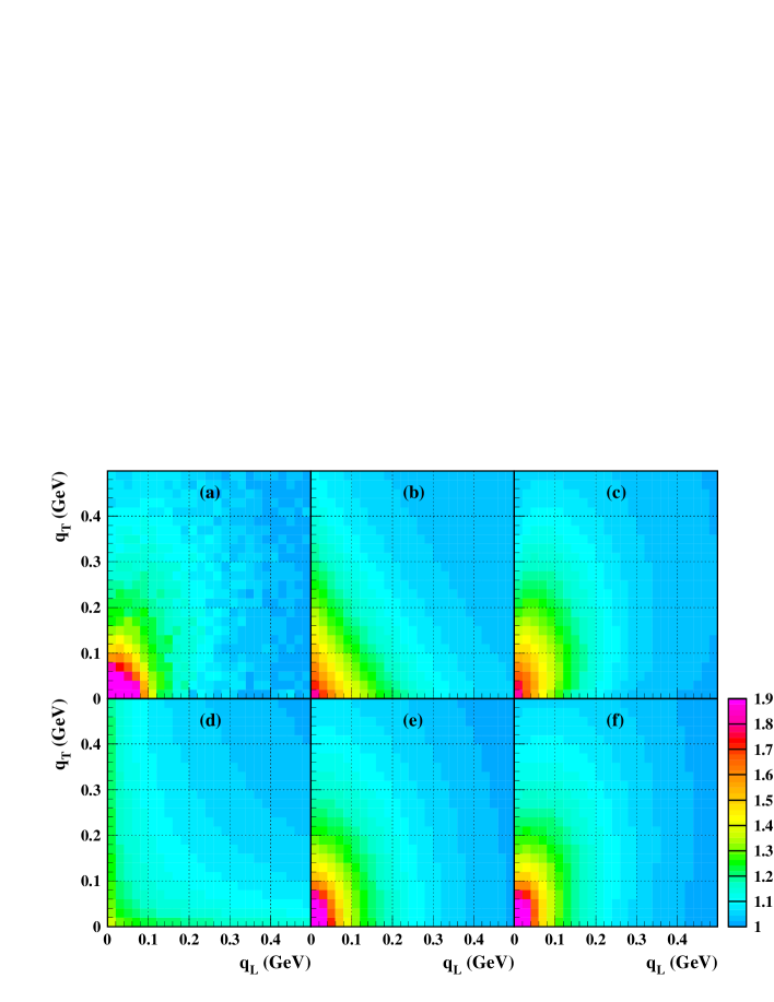
Figure 2: Shapes of $R_{2}(q_{L},q_{T})$ data and fits at intermediate scales. Panels show (a) UA1 data, (b) exponential, (c) exponential with cross term (d) power-law, (e) Lévy, (f) Lévy with cross term. Plots are truncated vertically to $R_{2}\leq 1.9$ to highlight structure at intermediate scales.

References

- [1] U. Heinz and B. V. Jacak, Ann. Rev. Nucl. Part. Sci. 49 (1999) 529.
- [2] T. Csörgő, Heavy Ion Physics 15 (2000) 1.
- [3] M. Lisa, S. Pratt, R. Soltz and U. A. Wiedemann, Ann. Rev. Nucl. Part. Sci. 55 (2005) 357; nucl-ex/0505014.
- [4] G.F. Bertsch, M. Gong and M. Tohyama, Phys. Rev. C 37 (1988) 1896.
- [5] UA1 Collaboration; A. Astbury et al., Nucl. Instr. Meth. 238 (1985) 288.
- [6] B. Buschbeck, H. C. Eggers and P. Lipa, Phys. Lett. B 481 (2000) 187; hep-ex/0003029.
- [7] UA1 Minimum Bias Collaboration, N. Neumeister et al., Phys. Lett. B 275 (1992) 186.
- [8] H. C. Eggers, P. Lipa and B. Buschbeck, Phys. Rev. Lett. 79 (1997) 197; hep-ph/9702235.
- [9] P. Lipa, PhD dissertation, University of Vienna (1990).
- [10] M.G. Bowler, Phys. Lett. B 270 (1991) 69.
- [11] D. Brinkmann, PhD Thesis, University of Frankfurt (1995).
- [12] P. Lipa, H.C. Eggers and B. Buschbeck, Phys. Rev. D 53 (1996) 4711; hep-ph/9604373.
- [13] S. Chapman, P. Scotto and U. Heinz, Phys. Rev. Lett. 74 (1995) 4400.
- [14] T. Csörgő, in: Proc. Cracow Workshop on Multiparticle Production, 1993, ed. by A. Białas, K. Fiałkowski, K. Zalewski and R.C. Hwa, World Scientific (1994); pp. 175–186.
- [15] STAR Collaboration, J. Adams et al., Phys. Rev. C 71 (2005) 044906, nucl-ex/0411036.
- [16] T. Csörgő, S. Hegyi and W. A. Zajc, Eur. Phys. J. C 36 (2004) 67; nucl-th/0310042.
- [17] S. Chapman, J. R. Nix and U. Heinz, Phys. Rev. C 52 (1995) 2694.
- [18] T. Csörgő, B. Lörstad and J. Zimányi, Z. Phys. C 71 (1994) 491; hep-ph/9411307.
- [19] R. Lednitsky and M.I. Podgoretzkii, Sov. J. Nucl. Phys. 30 (1979) 432.
- [20] EHS/NA22 Collaboration, N.M. Agababyan et al., Z. Phys. C 59 (1993) 195.
- [21] P. Carruthers, H.C. Eggers, and I. Sarcevic, Phys. Lett. B 254 (1991) 258.
- [22] UA1 Minimum Bias Collaboration, N. Neumeister et al., Z. Phys. C 60 (1993) 633.
- [23] AFS Collaboration, T. Åkesson et al., Phys. Lett. B 129 (1983) 269.
- [24] EHS/NA22 Collaboration, N. M. Agababyan et al., Z. Phys. C 68 (1995) 229.
- [25] EHS/NA22 Collaboration, N. M. Agababyan et al., Z. Phys. C 71 (1996) 405.
- [26] P. Danielewicz and S. Pratt, Phys. Lett. B 618 (2005) 60; nucl-th/0501003.
- [27] Z. Chajecki, T.D. Gutierrez, M.A. Lisa and M. Lopez-Noriega (STAR Collaboration), in: 21st Winter Workshop on Nuclear Dynamics, Breckenridge CO, February 2005, nucl-ex/0505009.
- [28] A. Bialas, Acta Phys. Polon. B 23 (1992) 561.
- [29] O. V. Utyuzh, G. Wilk, and Z. Wlodarczyk, Phys. Rev. D 61 (2000) 034007.