Abstract

We present a measurement of the $K$-$\pi$ vector current form-factor parameters for the decay $K_{L}\to\pi^{\pm}e^{\mp}\nu$. We use 328 pb^-1 of data collected in 2001 and 2002, corresponding to $\sim$ 2 million $K_{e3}$ events. Measurements of semileptonic form factors provide information about the dynamics of the strong interaction and are necessary for evaluation of the phase-space integral $I^{e}_{K}$ needed to measure the CKM matrix element $|V_{us}|$ for $K_{L}\to\pi^{\pm}e^{\mp}\nu$ decays. Our result is $\lambda_{+}=(28.6\pm 0.5\pm 0.4)10^{-3}$ for a linear fit, and $\mbox{$\lambda^{\prime}_{+}$}=(25.5\pm 1.5\pm 1.0)10^{-3}$, $\mbox{$\lambda^{\prime\prime}_{+}$}=(1.4\pm 0.7\pm 0.4)10^{-3}$ for a quadratic fit.
key words: ke3 form factor
PACS: 13.20.Eb

Measurement of the Form-Factor Slopes for the Decay $K_{L}\to\pi^{\pm}e^{\mp}\nu$ with the KLOE Detector

, , , , , , , , , , , , , , , , , , , , , , , , , , , , , , , , , , , , , , , , , , , , , , , , , , , , , , , , , , , , , , , , , , , , , , , , , , , , , , , , , , , , , ,

¹ Corresponding author: Mario Antonelli INFN - LNF, Casella postale 13, 00044 Frascati (Roma), Italy; tel. +39-06-94032728, e-mail mario.antonelli@lnf.infn.it

² Corresponding author: Marco Dreucci INFN - LNF, Casella postale 13, 00044 Frascati (Roma), Italy; tel. +39-06-94032696, e-mail marco.dreucci@lnf.infn.it

³ Corresponding author: Claudio Gatti INFN - LNF, Casella postale 13, 00044 Frascati (Roma), Italy; tel. +39-06-94032727, e-mail claudio.gatti@lnf.infn.it

1 Introduction

Semileptonic kaon decays, $K_{L}\to\pi^{\pm}\ell^{\mp}\nu$, (Fig. 1) offer possibly the cleanest way to obtain an accurate value of the Cabibbo angle, or better, $V_{us}$. Since $K\to\pi$ is a $0^{-}\to 0^{-}$ transition, only the vector part of the weak current has a nonvanishing contribution. The transition is therefore protected by the Ademollo-Gatto theorem against SU(3) breaking corrections to lowest order. At present, the largest uncertainty in calculating $V_{us}$ from the decay rate, is due to the difficulties in computing the matrix element $\langle\pi|j_{\mu}|K\rangle$.

Figure 1: Amplitude for $K_{L}\to\pi^{\pm}\ell^{\mp}\nu$. The gray region indicates the $K\to\pi W$ vertex structure.

In the electron mode $K_{L}\to\pi^{\pm}e^{\mp}\nu$ only one form factor is involved. In the following we will use the notation shown in Fig. 1, in which $P$, $p$, $k$ and $k^{\prime}$ are the kaon, pion, electron and neutrino momenta, respectively; $m$ is the mass of the charged pion and $M$ that of the neutral kaon. Terms in $(P-p)_{\mu}$ that acquire factor of $m_{e}$ are neglected. Therefore:

$$\langle\pi|J^{V}_{\mu}|K\rangle = f_{+}(t)(P+p)_{\mu}$$

We replace the form factor above with $f_{+}(0)\,\mbox{$\hat{f}_{+}(t)$}$, where $t=(P-p)^{2}=(k+k^{\prime})^{2}=M^{2}+m^{2}-2ME_{\pi}$ is the only L-invariant variable and $\mbox{$\hat{f}_{+}$}(0)=1$. The form factor is dominated by the vector $K$-$\pi$ resonances, the closest being the $K^{*}(892)$. Note that for $t>0$, $\hat{f}_{+}(t)$ $>1$. The presence of the form factor increases the value of the phase-space integral and the decay rate. The natural form for $\hat{f}(t)$ is

$$\mbox{$\hat{f}_{+}(t)$}={M_{V}^{2}\over M_{V}^{2}-t}.$$ (1)

It is also customary to expand the form factor as

$$\mbox{$\hat{f}_{+}(t)$}=1+\mbox{$\lambda^{\prime}_{+}$}~{}\frac{t}{m^{2}}+\frac{1}{2}\;\mbox{$\lambda^{\prime\prime}_{+}$}\,\left(\frac{t}{m^{2}}\right)^{2}\,+\dots$$ (2)

In the following we retain linear and quadratic terms. Note that the expansion of the pole form above gives $\mbox{$\lambda^{\prime}_{+}$}=(m/M_{V})^{2}$ and $\mbox{$\lambda^{\prime\prime}_{+}$}=2\,\mbox{$\lambda^{\prime}_{+}$}^{2}$. From $P+p=2P-(k+k^{\prime})$, and neglecting the $k+k^{\prime}$ term which is also proportional to $m_{e}$, the amplitude is:

$$\hbox{\euler M}=\langle\pi e\nu|H_{W}|K\rangle=2\frac{V_{us}G_{F}f_{+}(0)}{\sqrt{2}}P_{\mu}\bar{u}(k)\gamma^{\mu}(1-\gamma^{5})u(k^{\prime})\mbox{$\hat{f}_{+}(t)$}.$$ (3)

Squaring, summing over spins, and integrating over all variables but the pion energy, we obtain the pion spectrum

$$g(z)\propto\,\left(z^{2}-4\,\alpha\right)^{3\over 2}\,\left(1+{\lambda_{+}^{\prime}\over\alpha}\,\left(\xi-z\right)+{\lambda_{+}^{\prime\prime}\over 2\,\alpha^{2}}\,\left(\xi-z\right)^{2}\right)^{2}$$

where $\alpha=m^{2}/M^{2},\ \xi=1+\alpha$ and $z=2\,E_{\pi}/M$ is the normalized pion energy. The spectrum can also be written in terms of $t=m^{2}(\xi-z)/\alpha$ as

 

$${h(t)}$$

  (4)

2 The KLOE detector

The KLOE detector consists of a large, cylindrical drift chamber (DC), surrounded by a lead/scintillating-fiber electromagnetic calorimeter (EMC). A superconducting coil around the calorimeter provides a 0.52 T field. The drift chamber [1] is 4 m in diameter and 3.3 m long. The momentum resolution is $\sigma_{p_{\perp}}/p_{\perp}\approx 0.4\%$. Two-track vertices are reconstructed with a spatial resolution of $\sim$ 3 mm. The calorimeter [2] is divided into a barrel and two endcaps. It covers 98% of the solid angle. Cells close in time and space are grouped into calorimeter clusters. The energy and time resolutions are $\sigma_{E}/E=5.7\%/\sqrt{E\ {\rm(GeV)}}$ and $\sigma_{t}=57\ {\rm ps}/\sqrt{E\ {\rm(GeV)}}\oplus 100\ {\rm ps}$, respectively. The KLOE trigger [3] uses calorimeter and chamber information. For this analysis, only the calorimeter signals are used. Two energy deposition above threshold ($E>50$ MeV for the barrel and $E>150$ MeV for the endcaps) are required. Recognition and rejection of cosmic-ray events is also performed at the trigger level. Events with two energy deposition above a 30 MeV threshold in the outermost calorimeter plane are rejected.

3 Analysis

The 328 pb^-1 of 2001-2002 data used in this analysis [4], is divided into 14 periods of about 25 pb^-1/period. For each data period we have a corresponding sample of Monte Carlo events with approximately the same statistics.

Candidate $K_{L}$ events are tagged by the presence of a $K_{S}\to\pi^{+}\pi^{-}$ decay. The $K_{L}$ tagging algorithm is fully described in [5] and [6]. The $K_{L}$ momentum, $p_{K_{L}}$, is obtained from the kinematics of the $\phi\to K_{S}K_{L}$ decay, using the $K_{S}$ direction reconstructed from the measured momenta of the decay tracks and the known value of $\mathbf{p}_{\phi}$. The resolution is dominated by the beam-energy spread, and amounts to about 0.8 MeV/c. The position of the $\phi$ production point, $\mathbf{x}_{\phi}$, is determined as the point of closest approach of the $K_{S}$, propagated backward from the $K_{S}$ vertex, to the beam line. The $K_{L}$ line of flight (tagging line) is then constructed from the $K_{L}$ momentum, $\mathbf{p}_{K_{L}}=\mathbf{p}_{\phi}-\mathbf{p}_{K_{S}}$, and the position of the production vertex, $\mathbf{x}_{\phi}$.

The efficiency of the tagging procedure depends slightly on the evolution of the $K_{L}$, mainly because the trigger efficiency depends on the $K_{L}$ behavior. To identify events in which the $K_{S}$ by itself satisfies the calorimeter trigger, we require the presence of two clusters from the $K_{S}\to\pi^{+}\pi^{-}$ decay associated with fired trigger sectors (autotrigger). The value of the tagging efficiency obtained from Monte Carlo is about 40 % and is independent of $t$ to within 0.4%.

All tracks in the chamber, after removal of those from the $K_{S}$ decay and their descendants, are extrapolated to their points of closest approach to the tagging line. For each track candidate, we evaluate the point of closest approach to the tagging line, $\mathbf{x}_{\mathrm{c}}$, and the distance of closest approach, $d_{\mathrm{c}}$. The momentum $\mathbf{p}_{\mathrm{c}}$ of the track at $\mathbf{x}_{\mathrm{c}}$ and the extrapolation length $l_{\mathrm{c}}$ are also computed. Tracks satisfying $d_{\mathrm{c}}<ar_{xy}+b$, with $a=0.03$ and $b=3$ cm, and $-20$ cm $<l_{\mathrm{c}}<25$ cm are accepted as $K_{L}$ decay products, where $r_{xy}$ is the distance of the vertex from the origin in the transverse plane. For each sign of charge we consider the track with the smallest value of $d_{\mathrm{c}}$to be associated to the $K_{L}$ decay. Starting from these track candidates a vertex is reconstructed. The combined tracking and vertexing efficiency for $K_{e3}$ decays is about 54%. It is determined from data as described in LABEL:KLOE:brlnote. An event is retained if the vertex is in the fiducial volume $35<r_{xy}<150$ cm and $|z|<120$ cm.

To remove background from $K_{L}\to\pi^{+}\pi^{-}\pi^{0}$ and $K_{L}\to\pi^{+}\pi^{-}$ decays with minimal efficiency loss, we apply loose kinematic cuts: assuming the two tracks to have the pion mass, we require $E^{2}_{miss}-p^{2}_{miss}-M^{2}_{\pi^{0}}<-5000~{}{\rm\,Me\kern-1.25ptV}^{2}$ and $\sqrt{E^{2}_{miss}+p^{2}_{miss}}>10{\rm\,Me\kern-1.25ptV}$, where $E_{miss}$ and $p_{miss}$ are the missing energy and momentum, respectively. A large amount of background from $K_{L}\to\pi\mu\nu$ decays is rejected using $\Delta_{\pi\mu}$, the lesser value of $|\mbox{$E_{miss}-p_{miss}$}|$ calculated in the two hypotheses, $\pi\mu$ or $\mu\pi$. We retain events only if this variable is greater than 10 MeV. After the kinematic cuts described above, the efficiency for the signal is about 96%.

These kinematic criteria do not provide enaugh suppression of the background from $K_{L}\to\pi^{\pm}e^{\mp}\nu$ decays with incorrect charge assignment and from $K_{L}\to\pi\mu\nu$ decays. We make use of time-of-flight (TOF) information to further reduce the contamination.

For the purpose of track-to-cluster association, we define two quantities related to the distance between the track, extrapolated to the entry point of the calorimeter, and the closest cluster: $\it{d}_{\mathrm{TC}}$, the distance from the extrapolated entry point on the calorimeter to the cluster centroid and $\it{d}_{\mathrm{TC}\bot}$, the component of this distance in the plane transverse to the momentum of the track at the entry position. We only consider clusters with $\it{d}_{\mathrm{TC}\bot}$ $<$ 30 cm and $E>$50  MeV.

We evaluate the cluster efficiency using the Monte Carlo, and correct it with the ratio of data and Monte Carlo efficiencies obtained from control samples. A sample of $K_{e3}$ events with a purity of 99.5% is selected by means of kinematics and independent calorimeter information. Figure 2 shows the corrections as a function of $t$ obtained for a single run period.

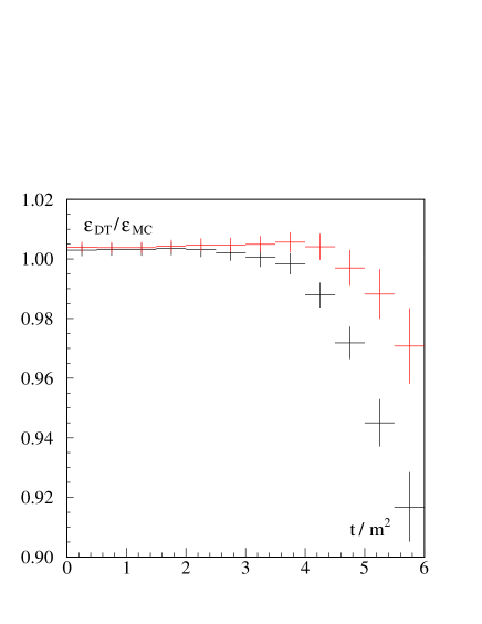
Figure 2: Cluster efficiency correction for pions ($\pi^{-}$ in red, $\pi^{+}$ in black) on the end cap from control sample. The plot refers to a single period of data taking

It is worth emphasizing that if this correction were not taken into account, the effect on $\lambda^{\prime}_{+}$ would be large (about 20%) and would produce different results for each charge (about 15%). For this reason, the analysis is performed separately for each charge. The comparison of the two results provides a first check of the validity of the corrections.

For each $K_{L}$ decay track with an associated cluster, we define the variable: $\Delta t_{i}=t_{\rm cl}-t_{i},~{}(i=\pi,~{}e)$ in which $t_{\rm cl}$ is the cluster time and $t_{i}$ is the expected time of flight, evaluated according to a well-defined mass hypothesis. The evaluating of $t_{i}$ includes the propagation time from the entry point to the cluster centroid [7]. We determine the $e^{+}e^{-}$ collision time, $t_{0}$, using the clusters from the $K_{S}$.

An effective way to select the correct mass assignment, $\pi e$ or $e\pi$, is obtained by choosing the lesser of $|\Delta t_{\pi^{+}}-\Delta t_{e^{-}}|$ and $|\Delta t_{\pi^{-}}-\Delta t_{e^{+}}|$. After the mass assignment has been made, we consider the variables $\Delta t_{\pi}+\Delta t_{e}$ and $\Delta t_{\pi}-\Delta t_{e}$. These are shown in Fig. 3 for signal and background Monte Carlo events. We select the signal by using a $2\sigma$ cut, where the resolution $\sigma\simeq 0.5~{}\mbox{ns}$.

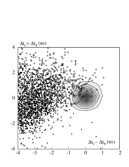
Figure 3: Monte Carlo distribution of $\Delta t_{e}+\Delta t_{\pi}$ versus $\Delta t_{e}-\Delta t_{\pi}$. Signal (gray scale), background from opposite sign $K_{L}\to\pi^{\pm}e^{\mp}\nu$ (black dot), background from same sign $K_{L}\to\pi\mu\nu$ (empty box).

After the TOF cut we have a contamination of $\sim$0.7%, almost entirely due to $K_{L}\to\pi\mu\nu$ decays.

We take the TOF efficiency from the Monte Carlo after correcting the time response of the calorimeter using data control samples [7]. The quality of this correction can be checked by comparing the data and Monte Carlo distributions for $\Delta t_{e}$ and $\Delta t_{\pi}$ shown in Fig. 4, obtained from the same control sample used for the cluster efficiency.

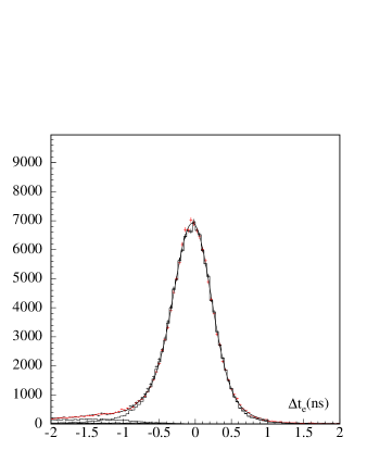
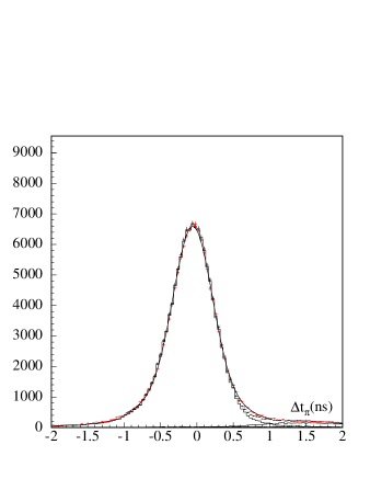
(a)	(b)

Figure 4: $\Delta t_{i}$ for electron (a) and pion (b) for data (black) and Monte Carlo (red)

We measure the form-factor slope parameters by fitting the distribution of the selected events in $t/m^{2}$. We modify the kinematic range of $t/m^{2}$, varying from $(m_{e}/m)^{2}\sim 10^{-5}$ up to $(M-m)^{2}/m^{2}\sim$ 6.8, to [-0.5,6], to take into account the smearing effect at $t\sim 0$ and the low statistics at high values of $t$. After subtracting the residual background as estimated from Monte Carlo, we perform the fit using the following formula:

$$\frac{dN}{dt}(i)=N_{0}\sum_{j=1}^{20}A(i,j)\times~{}\rho(j,\mbox{$\lambda^{\prime}_{+}$},\mbox{$\lambda^{\prime\prime}_{+}$})\times~{}\epsilon_{tot}(j)\times~{}F_{FSR}(j)$$ (5)

where $\rho(j,\mbox{$\lambda^{\prime}_{+}$},\mbox{$\lambda^{\prime\prime}_{+}$})$ is the three-body differential decay width as defined in Eq. (4), and $A(i,j)$ is the probability that an event with true value of $t/m^{2}$ in the $j^{\mathrm{th}}$ bin has a reconstructed value in the $i^{\mathrm{th}}$ bin. The chosen bin size is 0.5, which corresponds to about 1.6 $\sigma_{t}$, where $\sigma_{t}$ is the resolution in $t/m^{2}$.

The total efficiency, $\epsilon_{\rm{tot}}(t)$, takes into account the acceptance and the efficiency of the analysis cuts. $F_{\rm{FSR}}$ is the correction for final-state radiation. It is evaluated using the KLOE  Monte Carlo simulation, GEANFI  [8], where FSR processes are simulated according the procedures described in LABEL:KLOE:gattip. FSR affects the $t$-distribution mainly for high-energy pions, i.e. for low $t$, where the correction is 3-5%. The slopes $\lambda^{\prime}_{+}$ and $\lambda^{\prime\prime}_{+}$ are free parameters in the fit while the $N_{0}$ constant is the total number of signal events.

4 Systematic uncertainties

The systematic errors due to the evaluation of corrections, data-Monte Carlo inconsistencies, result stability, momentum miscalibration, and background contamination are summarized in Table 1.

	Linear fit	Quadratic fit
Source	$\delta\lambda_{+}\times 10^{3}$	$\delta\mbox{$\lambda^{\prime}_{+}$}\times 10^{3}$	$\delta\mbox{$\lambda^{\prime\prime}_{+}$}\times 10^{3}$
Tagging	0.14	0.18	0.02
Tracking and vertexing	0.16	0.22	0.18
Clustering	0.07	0.24	0.13
Time-of-flight	0.29	0.87	0.27
Background	0.08	0.16	0.03
Momentum-scale	0.06	0.05	0.05
Momentum-resolution	0.17	0.22	0.19
Total systematic	0.42	0.98	0.39

Table 1: Summary of systematic uncertainties on $\lambda_{+}$, $\lambda^{\prime}_{+}$and $\lambda^{\prime\prime}_{+}$.

We evaluate the systematic uncertainty of the tagging efficiency by repeating the measurement using a tagging algorithm without the requirement of the autotrigger. We observe a change of 0.14$\times 10^{-3}$ for $\lambda_{+}$ in the case of the linear fit, and changes of 0.18$\times 10^{-3}$ and 0.02$\times 10^{-3}$ for $\lambda^{\prime}_{+}$ and $\lambda^{\prime\prime}_{+}$ respectively for the quadratic fit.

We evaluate the systematic uncertainties on the tracking efficiency corrections by checking stability of the result when the track selection criteria are modified. We establish the validity of the method by comparing the efficiencies from data and Monte Carlo control samples, and from the Monte Carlo truth [7]. The uncertainty on the tracking efficiency correction is dominated by sample statistics and by the variation of the results observed using different criteria to identify tracks from $K_{L}$ decays. The correction is run-period dependent; its statistical error is taken into account in the fit. We study the effect of differences in the resolution with which the variable $d_{\mathrm{c}}$ is reconstructed in data and in Monte Carlo events, and the possible bias introduced in the selection of the control sample, by varying the values of the cuts made on this variable when associating tracks to $K_{L}$ vertices. For each variation, corresponding to a maximal change of the tracking efficiency of about $\pm$15%, we evaluate the complete tracking-efficiency correction and measure the slope parameters. We observe a change of 0.16$\times 10^{-3}$ for $\lambda_{+}$ in the case of the linear fit, and changes of 0.22$\times 10^{-3}$ and 0.18$\times 10^{-3}$ for $\lambda^{\prime}_{+}$ and $\lambda^{\prime\prime}_{+}$ , respectively, for the quadratic fit. We find a smaller uncertainty by comparing the efficiencies from data and Monte Carlo control samples, and Monte Carlo truth. However, we conservatively assume the systematic uncertainty to be given by the changes in the result observed by varying the cut on $d_{\mathrm{c}}$.

We evaluate the systematic uncertainties on the clustering efficiency corrections by checking stability of the result when the track-to-cluster association criteria are modified. In this case as well, the uncertainties on the clustering efficiency corrections are dominated by sample statistics and by the variation of the results observed using different criteria for the track-to-cluster association. The correction is run-period dependent; we take into account its statistical error in the fit. The most effective variable in the definition of track-to-cluster association is the transverse distance, $\it{d}_{\mathrm{TC}\bot}$. We vary the cut on $\it{d}_{\mathrm{TC}\bot}$  in a wide range from 7 cm to 30 cm, corresponding to a change in efficiency of about 17%. For each configuration, we obtain the complete track extrapolation and clustering efficiency correction and use it to evaluate the slopes. We observe a variation of 0.07$\times 10^{-3}$ for $\lambda_{+}$ in the case of the linear fit, and variations of 0.24$\times 10^{-3}$ and 0.13$\times 10^{-3}$ for $\lambda^{\prime}_{+}$ and $\lambda^{\prime\prime}_{+}$ , respectively, in the case of the quadratic fit. We find a comparable uncertainty for $\lambda^{\prime}_{+}$ and for $\lambda^{\prime\prime}_{+}$ by comparing the efficiencies from data and Monte Carlo control samples, and the Monte Carlo truth.

We study the uncertainty on the Monte Carlo efficiency of the TOF selection procedure by measuring it using a pure $K_{e3}$ control sample, and using the ratio of data and Monte Carlo efficiencies estimated in this way as a correction. The control sample is selected using tighter kinematic cuts and the calorimeter particle identification described in LABEL:KLOE:brlnote. The contamination of the control sample amounts to 0.4%. When applying the correction, we find a change in the result of 0.29$\times 10^{-3}$ for $\lambda_{+}$ in the case of the linear fit, and changes of 0.87$\times 10^{-3}$ and 0.27$\times 10^{-3}$ for $\lambda^{\prime}_{+}$ and $\lambda^{\prime\prime}_{+}$ , respectively, in the case of the quadratic fit. These variations are well within the statistical uncertainties.

We study the uncertainties on the background evaluation by repeating the measurement on a sample with reduced background contamination. This is achived by identifying the electron using the energy deposition in the calorimeter combined with a neural network (NN). In Fig. 5 we show the distribution of the NN output for the sample used in the analysis. Requiring the value of the NN output to be greater than 0.4, we reduce the background contamination by about a factor of three.

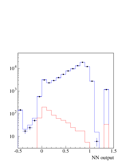
Figure 5: NN output distribution for data (dots), Monte Carlo signal (black solid line) and background (red solid line).

The differences in the result obtained with this cut are 0.08$\times 10^{-3}$ for $\lambda_{+}$ in the case of the linear fit, and 0.16$\times 10^{-3}$ and 0.03$\times 10^{-3}$ for $\lambda^{\prime}_{+}$ and $\lambda^{\prime\prime}_{+}$ , respectively, in the case of the quadratic fit.

The effect of the momentum scale uncertainty and the momentum resolution have also been considered. We find the following relations by changing the momentum scale:

$$\frac{\delta\mbox{$\lambda^{\prime}_{+}$}}{\mbox{$\lambda^{\prime}_{+}$}}\simeq-2\frac{\delta p}{p},~{}~{}~{}~{}\frac{\delta\mbox{$\lambda^{\prime\prime}_{+}$}}{\mbox{$\lambda^{\prime\prime}_{+}$}}\simeq-4\frac{\delta p}{p}$$

We conservatively assume a momentum scale uncertainty of 0.1%, which is much greater than the value obtained from a dedicated analysis [10]. This translates into a change of 0.06$\times 10^{-3}$ for $\lambda_{+}$ in the case of the linear fit, and changes of 0.05$\times 10^{-3}$ and 0.05$\times 10^{-3}$ for $\lambda^{\prime}_{+}$ and $\lambda^{\prime\prime}_{+}$ , respectively, in the case of the quadratic fit.

We investigate the effect of the momentum resolution by changing the value of the resolution on $t/m^{2}$. A variation of 3% worsens the fit quality, giving a $\chi^{2}$ probability variation of one standard deviation. The corresponding absolute changes are 0.17$\times 10^{-3}$ for $\lambda_{+}$ in the case of the linear fit, and 0.22$\times 10^{-3}$ and 0.19$\times 10^{-3}$ for $\lambda^{\prime}_{+}$ and $\lambda^{\prime\prime}_{+}$ in the case of quadratic fit. Varying the resolution of $t/m^{2}$ by a larger amount (6%) gives an unacceptable $\chi^{2}$ probability, about $10^{-9}$, while nearly the same variations for the fit parameters are observed. In principle, if the distribution has a linear behavior, the slope is insensitive to any smearing due to the resolution. The only effect is due to the depletion of the bins at the boundary of the distribution, which worsens the $\chi^{2}$ of the fit. We have verified that the sensitivity to the momentum resolution is much smaller for a reduced fit range.

5 Results

About 2 million $K_{e3}$ events were selected. The results of the linear fit obtained from all run periods are given in Table 2. The fit is performed separately for $K_{L}\to\pi^{+}e^{-}\overline{\nu}$ and $K_{L}\to\pi^{-}e^{+}\nu$ events to check the reliability of the evaluation of the cluster efficiency. The results are consistent only if the respective efficiency corrections for each pion charge are applied. Then, combining the two charge results and including the systematic uncertainties listed in Table 1 we obtain:

$$\lambda_{+} = (28.6\pm 0.5_{\rm{stat.}}\pm 0.4_{\rm{syst.}})\times\rm{10^{-3}}$$

The results obtained for the quadratic fit are given in Table 3. A correlation of $\sim-0.95$ between the $\lambda^{\prime}_{+}$ and $\lambda^{\prime\prime}_{+}$ parameters is obtained, as expected from the form of the parametrization in Eq. (2). A very slight preference for a small quadratic term is observed as indicated by the small improvement in the fit probability going from the linear, P$(\chi^{2})=89$%, to the quadratic fit P$(\chi^{2})=92$%. Including the systematic uncertainties listed in Table 1 we obtain:

$$\lambda^{\prime}_{+} = (25.5\pm 1.5_{\rm{stat.}}\pm 1.0_{\rm{syst.}})\times\rm{10^{-3}}$$

$$\lambda^{\prime\prime}_{+} = (1.4\pm 0.7_{\rm{stat.}}\pm 0.4_{\rm{syst.}})\times\rm{10^{-3}}$$

Figure 6 shows the $t/m^{2}$ distribution for the data and the fit result. The ratio data/fit is also shown.

Linear fit	$\lambda_{+}\times 10^{3}$	$\chi^{2}/\rm{ndf}$
$K_{L}\to\pi^{-}e^{+}\nu$	$28.7\pm 0.7$	$156/181$
$K_{L}\to\pi^{+}e^{-}\overline{\nu}$	$28.5\pm 0.6$	$174/181$
Combined	$28.6\pm 0.5$	$330/363$

Table 2: Fit results in the hypothesis $\lambda^{\prime\prime}_{+}$=0. Only statistical errors are shown.

Quadratic fit	$\mbox{$\lambda^{\prime}_{+}$}\times 10^{3}$	$\mbox{$\lambda^{\prime\prime}_{+}$}\times 10^{3}$	$\chi^{2}/\rm{ndf}$
$K_{L}\to\pi^{-}e^{+}\nu$	$24.6\pm 2.1$	$1.9\pm 1.0$	$152/180$
$K_{L}\to\pi^{+}e^{-}\overline{\nu}$	$26.4\pm 2.1$	$1.0\pm 1.0$	$173/180$
Combined	$25.5\pm 1.5$	$1.4\pm 0.7$	$325/362$

Table 3: Fit results with $\lambda^{\prime}_{+}$ and $\lambda^{\prime\prime}_{+}$ as free parameters. Only statistical errors are shown.

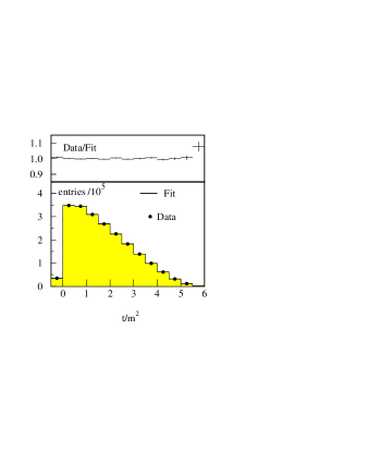
(a) Linear fit	(b) Quadratic fit

Figure 6: Fit results: data (dots) are superimposed on the fit function (histogram). The data/Fit ratio is also shown.

We also fit the data using the one-pole parametrization (see Eq. (1)). We obtain $M_{V}=(870\pm 6){\rm\,Me\kern-1.25ptV}$ with $\chi^{2}/\rm{ndf}=326/364$ and a probability of P$(\chi^{2})=92.4$%. Taking the systematic error into account, we obtain:

$$M_{V} = (870\pm 6_{\rm{stat.}}\pm 7_{\rm{syst.}}){\rm\,Me\kern-1.25ptV}$$

This result indicates that, although the pole is dominated by the $K^{*}$ vector meson, contributions from other $J^{P}=1^{-}$ resonant and non-resonant $K\pi$ scattering amplitudes are not negligible.

Conclusion

We have obtained precise new values of the slopes used to describe the hadronic form factor in $K_{e3}$ decay. The new KLOE result is consistent with the presence of a small quadratic term in agreement with the expectation of the one-pole expansion. The value of $\lambda_{+}$ obtained with the linear fit is in good agreement with other existing measurements. The comparison with other existing measurements is shown in Fig. 7 in the case of the quadratic fit. Our result is in good agreement with ISTRA+ [11] and NA48  [12] and in marginal disagreement with KTeV [13].

Figure 7: Comparison of present results with other recent measurements  [11, 12, 13]. The black dot represents the values of $\lambda^{\prime}_{+}$ and $\lambda^{\prime\prime}_{+}$ obtained from the Taylor expansion of the pole parametrization. The ISTRA+ result is corrected with the ratio $(m_{\pi^{+}}/m_{\pi^{0}})^{2}$.

References

- [1] M. Adinolfi, et al., The tracking detector of the KLOE experiment, Nucl. Instrum. Meth. A 488 (2002) 51.
- [2] M. Adinolfi, et al., The KLOE electromagnetic calorimeter, Nucl. Instrum. Meth. A 482 (2002) 364.
- [3] M. Adinolfi, et al., The trigger system of the KLOE experiment, Nucl. Instrum. Meth. A 492 (2002) 134.
-
[4]
M. Antonelli, M. Dreucci, C. Gatti, Measurement of the Semileptonic
Form Factor Slope and Curvature and Pole in the Decay at
KLOE, KLOE Note 210 (2006).
URL http://www.lnf.infn.it/kloe/pub/knote/kn210.ps -
[5]
M. Antonelli, P. Beltrame, M. Dreucci, M. Moulson, M. Paultan, A. Sibidanov,
Measurements of the Absolute Branching Ratios for Dominant Decays, the
Lifetime, and with the Kloe Detector, KLOE Note 204 (2005).
URL http://www.lnf.infn.it/kloe/pub/knote/kn204.ps.gz - [6] KLOE Collaboration, F. Ambrosino, et al., Phys. Lett. B 632 (2006) 43.
- [7] KLOE Collaboration, F. Ambrosino, et al., Measurement of the branching fraction and charge asymmetry for the decay with the KLOE detector, hep-ex/0601026, Submitted to Phys. Lett. B, and references therein .
- [8] F. Ambrosino, et al., Data handling, reconstruction, and simulation for the KLOE experiment, Nucl. Instrum. Meth. A 534 (2004) 403.
- [9] C. Gatti, Monte Carlo simulation for radiative kaon decays, hep-ph/0507280, accepted by Eur. Phys. J. C, and references therein .
- [10] A. Antonelli, et al., The KLOE field map revisited, KLOE Memo 233 (2001).
- [11] O. P. Yushchenko, et al., Phys. Lett. B 589 (2004) 111.
- [12] NA48 Collaboration, A. Lai, et al., Phys. Lett. B 606 (2004) 1.
- [13] KTeV Collaboration, T. Alexopolous, et al., Phys. Rev. D 70 (2004) 092007.