Study of the branching ratio and charge asymmetry for the decay $K_{S}\rightarrow\pi e\nu$ with the KLOE detector

Abstract

Among some 400 million $K_{S}$$K_{L}$ pairs produced in $e^{+}e^{-}$ annihilations at DAΦNE, $\sim$ 6500 each of $K_{S}$$\rightarrow$$\pi^{+}e^{-}\bar{\nu}$ and $K_{S}$$\rightarrow$$\pi^{-}e^{+}\nu$ decays have been observed with the KLOE detector. From these, the ratio $\Gamma(K_{S}\rightarrow\pi e\nu)/\Gamma(K_{S}\rightarrow\pi^{+}\pi^{-})\!=\!(10.19\pm 0.13)\times 10^{-4}$ is obtained, improving the accuracy on $\mathrm{BR}(K_{S}\rightarrow\pi e\nu)$ by a factor of four and providing the most precise test of the $\Delta S\!=\!\Delta Q$ rule. From the partial width $\Gamma(K_{S}\rightarrow\pi e\nu)$, a value for $f_{+}^{K^{0}}(0)\!\times\!V_{us}$ is obtained that is in agreement with unitarity of the quark-mixing matrix. The lepton charge asymmetry $A_{S}\!=\!(1.5\pm 9.6_{\mathrm{stat}}\pm 2.9_{\mathrm{syst}})\times 10^{-3}$ is compatible with the requirements of $CPT$ invariance. The form-factor slope agrees with recent results from semileptonic $K_{L}$ and $K^{+}$ decays. These are the first measurements of the charge asymmetry and form-factor slope for semileptonic $K_{S}$ decays.

, , , , , , , , , , , , , , , , , , , , , , , , , , , , , , , , , , , , , , , , , , , , , , , , , , , , , , , , , , , , , , , , , , , , , , , , , , , , , , , , , , , , , ,

¹ Corresponding author: Claudio Gatti INFN - LNF, Casella postale 13, 00044 Frascati (Roma), Italy; tel. +39-06-94032727, e-mail claudio.gatti@lnf.infn.it

² Corresponding author: Tommaso Spadaro INFN - LNF, Casella postale 13, 00044 Frascati (Roma), Italy; tel. +39-06-94032698, e-mail tommaso.spadaro@lnf.infn.it

1 Introduction

Semileptonic kaon decays provide at present the best way to learn about $s,\>u$ quark couplings and allow tests of many fundamental aspects of the Standard Model (SM). Only the vector part of the weak current has a non-vanishing matrix element between a kaon and a pion. The vector current is “almost” conserved. For a vector interaction, there are no $SU(3)$-breaking corrections to first order in the $s$-$d$ mass difference [1], making calculations of hadronic matrix elements more reliable. Therefore, the CKM matrix element $V_{us}$ can be accurately extracted from the measurement of the semileptonic decay widths and the most precise test of unitarity of the CKM matrix can be obtained from the first-row constraint: $1\!-\!\Delta\!\simeq\!|V_{ud}|^{2}\!+\!|V_{us}|^{2}$. Using $V_{ud}$ from $0^{+}\!\to\!0^{+}$ nuclear beta decays, a test of the expectation $\Delta\!=\!0$ with a precision of one part per mil can be performed.

At a $\phi$ factory very large samples of tagged, monochromatic $K_{S}$ mesons are available. We have isolated a very pure sample of $\sim$13 000 semileptonic $K_{S}$ decay events and measured for the first time the partial decay rates for transitions to final states of each charge, $\Gamma(\mbox{$K_{S}$}\!\rightarrow\!e^{+}\pi^{-}\nu)$ and $\Gamma(\mbox{$K_{S}$}\!\rightarrow\!e^{-}\pi^{+}\bar{\nu})$, and the charge asymmetry

$$A_{S}=\frac{\Gamma\left(\mbox{$K_{S}$}\rightarrow\pi^{-}e^{+}\nu\right)-\Gamma\left(\mbox{$K_{S}$}\rightarrow\pi^{+}e^{-}\bar{\nu}\right)}{\Gamma\left(\mbox{$K_{S}$}\rightarrow\pi^{-}e^{+}\nu\right)+\Gamma\left(\mbox{$K_{S}$}\rightarrow\pi^{+}e^{-}\bar{\nu}\right)}.$$ (1)

The comparison of $A_{S}$ with the asymmetry $A_{L}$ for $K_{L}$ decays allows tests of the $CP$ and $CPT$ symmetries. Comparison of the $K_{S}$ and $K_{L}$ widths $\Gamma(K_{S}\rightarrow\pi e\nu)$ and $\Gamma(K_{L}\rightarrow\pi e\nu)$ allows a test of the validity of the $\Delta S\!=\!\Delta Q$ rule. Assuming $CPT$ invariance, $A_{S}\!=\!A_{L}\!=\!2\,\mathrm{Re}\,\epsilon\!\simeq\!3\!\times\!10^{-3}$, where $\epsilon$ gives the $CP$ impurity of the $K_{S}$, $K_{L}$ mass eigenstates due to $CP$ violation in $K\!\leftrightarrow\!\overline{K}$ $\Delta S=2$ transitions. The difference between the charge asymmetries,

$$A_{S}-A_{L}=4\,\left(\mathrm{Re}\,\delta+\mathrm{Re}\,x_{-}\right),$$ (2)

signals $CPT$ violation either in the mass matrix ($\delta$ term), or in the decay amplitudes with $\Delta S\!\neq\!\Delta Q$ ($x_{-}$ term). The sum of the asymmetries,

$$A_{S}+A_{L}=4\left(\mathrm{Re}\,\epsilon-\mathrm{Re}\,y\right),$$ (3)

is related to $CP$ violation in the mass matrix ($\epsilon$ term) and to $CPT$ violation in the $\Delta S\!=\!\Delta Q$ decay amplitude ($y$ term). Finally, the validity of the $\Delta S\!=\!\Delta Q$ rule in $CPT$-conserving transitions can be tested through the quantity:

$$\mathrm{Re}\,x_{+}=\frac{1}{2}\frac{\Gamma(K_{S}\rightarrow\pi e\nu)-\Gamma(K_{L}\rightarrow\pi e\nu)}{\Gamma(K_{S}\rightarrow\pi e\nu)+\Gamma(K_{L}\rightarrow\pi e\nu)}.$$ (4)

Writing the $K^{0}$ and $\hbox to0.0pt{\kern 1.99997pt\raise 8.61108pt\hbox to6.99997pt{\hrulefill}\hss}K\kern 1.0pt\vphantom{K}^{0}$ decay amplitudes for final states of each charge as ${\mathcal{A}}_{\pm}\!=\!A(K^{0}\!\rightarrow\!e^{\pm}\pi^{\mp}\nu(\bar{\nu}))$ and $\bar{{\mathcal{A}}}_{\pm}\!=\!A(\hbox to0.0pt{\kern 1.99997pt\raise 8.61108pt\hbox to6.99997pt{\hrulefill}\hss}K\kern 1.0pt\vphantom{K}^{0}\!\rightarrow\!e^{\pm}\pi^{\mp}\nu(\bar{\nu}))$, the above parameters are defined as follows:

  $${x_{\pm}} {{}=\frac{1}{2}\left[\frac{\bar{{\mathcal{A}}}_{+}}{{\mathcal{A}}_{+}}\pm\left(\frac{{\mathcal{A}}_{-}}{\bar{{\mathcal{A}}}_{-}}\right)^{\ast}\right],} {y} {{}=\frac{\bar{{\mathcal{A}}}_{-}^{\ast}-{\mathcal{A}}_{+}}{\bar{{\mathcal{A}}}_{-}^{\ast}+{\mathcal{A}}_{+}},}$$   (5a)

  $${\epsilon} {{}=i\frac{\mathrm{Im}M_{12}-i\mathrm{Im}\Gamma_{12}/2}{m_{S}-m_{L}-i(1/\tau_{S}-1/\tau_{L})/2},} {\delta} {{}=\frac{1}{2}\frac{M_{11}-M_{22}-i(\Gamma_{11}-\Gamma_{22})/2}{m_{S}-m_{L}-i(1/\tau_{S}-1/\tau_{L})/2},}$$   (5b)

where $M_{ij}$ and $\Gamma_{ij}$ are the elements of the mass and decay matrices describing the time evolution of the neutral kaon system, and $m_{S,L}$ and $\tau_{S,L}$ are respectively the masses and lifetimes for $K_{S,L}$.

The value of $A_{L}$ is known at present with an accuracy of $10^{-4}$ [2], while $A_{S}$ has never yet been measured. At present, the most precise test of $CPT$ conservation comes from the CPLEAR experiment [3]: they find $\mathrm{Re}\,\delta$ and $\mathrm{Re}\,x_{-}$ to be compatible with zero, with accuracies of $3\!\times\!10^{-4}$ and $10^{-2}$, respectively. The present value of $\mathrm{Re}\,y$, obtained from unitarity [4], is compatible with zero to within $3\!\times\!10^{-3}$.

In the SM, $\mathrm{Re}\,x_{+}$ is on the order of $G_{F}m_{\pi}^{2}\!\sim\!10^{-7}$, being due to second-order weak transitions. At present, the most precise test of the $\Delta S\!=\!\Delta Q$ rule comes from an analysis of the time distribution of strangeness-tagged semileptonic kaon decays at CPLEAR [5]. They found $\mathrm{Re}\,x_{+}$ to be compatible with zero to within $6\!\times\!10^{-3}$.

The most precise previous measurement of $\mathrm{BR}(K_{S}\rightarrow\pi e\nu)$ was obtained by KLOE using $\sim 20\!$pb^-1 of data collected in 2000 and has a fractional accuracy of 5.4% [6]. The present result is based on the analysis of 410 pb^-1 of data and improves on the total error by a factor of four, to 1.3%.

2 Measurement method

We measure $K_{S}$ branching ratios using kaons from $\phi\rightarrow K_{S}K_{L}$ decays. The data were collected with the KLOE detector at DAΦNE, the Frascati $\phi$-factory. DAΦNE is an $e^{+}e^{-}$ collider that operates at a center of mass energy of $\sim$1020 MeV, the mass of the $\phi$ meson. Equal-energy positron and electron beams collide at an angle of $\pi-25$ mrad, producing $\phi$ mesons with a small momentum in the horizontal plane: $p_{\phi}\!\sim 13\!{\rm\,M{e\kern-0.70007ptV}}.$ $\phi$ mesons decay $\sim\!34\%$ of the time into neutral kaons. $K_{L}$’s and $K_{S}$’s have mean decay paths of $\lambda_{L}\!\sim\!350$ cm and $\lambda_{S}\!\sim\!0.6$ cm, respectively.

The KLOE detector consists of a large cylindrical drift chamber surrounded by a lead/scintillating-fiber sampling calorimeter. A superconducting coil outside the calorimeter provides a 0.52 T field. The drift chamber [7], which is 4 m in diameter and 3.3 m long, has 12 582 cells strung in all-stereo geometry. The chamber shell is made of a carbon-fiber/epoxy composite. The chamber is filled with a 90% He, 10% iC₄H₁₀ mixture. These features maximize transparency to photons and reduce $K_{L}$$\rightarrow$$K_{S}$ regeneration. The spatial resolutions are $\sigma_{xy}\!\sim\!150\,\mathrm{\mu m}$ and $\sigma_{z}\!\sim\!2{\rm\,mm}.$ The momentum resolution is $\sigma_{p_{\perp})}/p_{\perp}\!\leq\!0.4\%$. Vertices are reconstructed with a spatial resolution of $\sim\!3{\rm\,mm}$. The calorimeter [8] is divided into a barrel and two endcaps and covers 98% of the solid angle. The energy resolution is $\sigma_{E}/E\!=\!5.7\%/\sqrt{E({\rm G{e\kern-0.70007ptV}})}$ and the timing resolution is $\sigma_{t}\!=\!57{\rm\,ps}/\sqrt{E({\rm G{e\kern-0.70007ptV}})}\oplus 100{\rm\,ps}$ [9]. The trigger used for the present analysis relies entirely on calorimeter information [10]. Two local energy deposits above threshold ($50$ MeV on the barrel, $150$ MeV on the endcaps) are required. The trigger time has a large spread with respect to the bunch-crossing period. However, it is synchronized with the machine RF divided by 4, $T_{\mathrm{sync}}\!\sim\!10.8{\rm\,ns}$, with an accuracy of 50 ps. As a result, the time $T_{0}$ of the bunch crossing producing an event, which is determined after event reconstruction, is known up to an integer multiple of the bunch-crossing time, $T_{\mathrm{bunch}}\!\sim\!2.7{\rm\,ns}$.

The main advantage of studying kaons at a $\phi$ factory is that $K_{L}$’s and $K_{S}$’s are produced nearly back-to-back in the laboratory so that detection of a $K_{L}$ meson tags the production of a $K_{S}$ meson and gives its direction and momentum. The contamination from $\mbox{$K_{L}$}\!\mbox{$K_{L}$}\!\gamma$ and $\mbox{$K_{S}$}\!\mbox{$K_{S}$}\!\gamma$ final states is negligible for our measurement [11, 12]. Since the branching ratio for $K_{S}\rightarrow\pi^{+}\pi^{-}$ is known with an accuracy of $\sim 0.1\%$ [13, 14], the $K_{S}\rightarrow\pi e\nu$ branching ratio is evaluated by normalizing the number of signal events, separately for each charge state, to the number of $K_{S}\rightarrow\pi^{+}\pi^{-}$ events in the same data set. This allows cancellation of the uncertainties arising from the integrated luminosity, the $\phi$ production cross section, and the tagging efficiency. The measurement is based on an integrated luminosity of 410 $\rm pb^{-1}$ at the $\phi$ peak collected during two distinct data-taking periods in the years 2001 and 2002, corresponding to $\sim\!1.3\times 10^{9}$ produced $\phi$-mesons. Since the machine conditions were different during the two periods, we have measured the branching ratios separately for each data set. Our final results are based on the averages of these measurements.

3 Selection criteria

About half of the $K_{L}$ mesons reach the calorimeter, where most interact. Such an interaction is called a $K_{L}$ crash in the following. A $K_{L}$ crash is identified as a local energy deposit with $E\!>\!200{\rm\,M{e\kern-0.70007ptV}}$ and a time of flight corresponding to a low velocity: $\beta\!\sim\!0.216$. The coordinates of the energy deposit determine the $K_{L}$ direction to within $\sim\!20$ mrad, as well as the momentum $\mathbf{p}_{L}$, which is weakly dependent on the $K_{L}$ direction because of the motion of the $\phi$ meson. A $K_{L}$ crash thus tags the production of a $K_{S}$ of momentum $\mathbf{p}_{S}\!=\!\mathbf{p}_{\phi}-\mathbf{p}_{L}$. $K_{S}$ mesons are tagged with an overall efficiency of $\sim\!20\%$. Both $K_{S}\rightarrow\pi e\nu$ and $K_{S}\rightarrow\pi^{+}\pi^{-}$ decays are selected from this tagged sample. Event selection consists of fiducial cuts, particle identification by time of flight, and kinematic closure.

Identification of a $K_{S}\rightarrow\pi^{+}\pi^{-}$ decay requires two tracks of opposite curvature. The tracks must extrapolate to the interaction point (IP) to within a few centimeters. The reconstructed momenta and polar angles must lie in the intervals $120{\rm\,M{e\kern-0.70007ptV}}\!<\!p\!<\!300{\rm\,M{e\kern-0.70007ptV}}$ and $30^{\circ}\!<\!\theta\!<\!150^{\circ}$. A cut in $(p_{\perp},p_{\parallel})$ selects non-spiralling tracks. The numbers of $K_{S}\rightarrow\pi^{+}\pi^{-}$ events found in each data set are shown in Tab. 1. Contamination due to $K_{S}$ decays other than $K_{S}\rightarrow\pi^{+}\pi^{-}$ is at the per-mil level and is estimated from Monte Carlo (MC).

	Year 2001	Year 2002
Luminosity, $\rm pb^{-1}$	$152\pm 1$	$286\pm 2$
Channel	Number of selected events
$K_{S}\rightarrow\pi^{+}\pi^{-}$	13 056 500	22 840 700
$\mbox{$K_{S}$}\to\pi^{+}e^{-}\bar{\nu}$	$2387\pm 52_{\mathrm{stat}}\pm 22_{\mathrm{syst}}$	$4238\pm 69_{\mathrm{stat}}\pm 55_{\mathrm{syst}}$
$\mbox{$K_{S}$}\to\pi^{-}e^{+}\nu$	$2541\pm 52_{\mathrm{stat}}\pm 24_{\mathrm{syst}}$	$4446\pm 71_{\mathrm{stat}}\pm 69_{\mathrm{syst}}$

Table 1: Number of selected $K_{S}\rightarrow\pi^{+}\pi^{-}$ and $K_{S}\rightarrow\pi e\nu$ decays for the 2001 and 2002 data sets.

Identification of a $K_{S}\rightarrow\pi e\nu$ event also begins with the requirement of two tracks of opposite curvature. The tracks must extrapolate and form a vertex close to the IP. The invariant mass $M_{\pi\pi}$ of the pair calculated assuming both tracks are pions must be smaller than 490 MeV. This rejects $\sim\!95\%$ of the $\pi^{+}\pi^{-}$ decays and $\sim\!10\%$ of the signal events.

We discriminate between electron and pion tracks by time of flight (TOF). The tracks are therefore required to be associated with calorimeter energy clusters. For each track, we compute the difference $\delta_{t}(m)\!=\!t_{\mathrm{cl}}-L/c\beta(m)$ using the cluster time $t_{\mathrm{cl}}$ and the track length $L$. The velocity $\beta$ is computed from the track momentum for each mass hypothesis, $m\!=\!m_{e}$ and $m\!=\!m_{\pi}$. In order to avoid uncertainties due to the determination of $T_{0}$ (the time of the bunch crossing producing the event), we make cuts on the two-track difference

$$\mathrm{d}\delta_{t,ab}=\delta_{t}(m_{a})_{1}-\delta_{t}(m_{b})_{2}\mbox{,}$$

where the mass hypothesis $m_{a(b)}$ is used for track 1(2). This difference is zero for the correct mass assignments. First, $K_{S}\rightarrow\pi^{+}\pi^{-}$ events are rejected by requiring $|\mathrm{d}\delta_{t,\pi\pi}|\!>\!1.7$ ns. Then, the differences $\mathrm{d}\delta_{t,\pi e}$ and $\mathrm{d}\delta_{t,e\pi}$ are calculated for surviving events. The scatter plot of the two variables is shown in Fig. 1 for Monte Carlo events. The cuts applied on these time differences for the selection of $K_{S}\rightarrow\pi e\nu$ events are illustrated in the figure: $|\mathrm{d}\delta_{t,\pi e}|\!<\!1.4$ ns, $\mathrm{d}\delta_{t,e\pi}\!>\!3.2$ ns; or $|\mathrm{d}\delta_{t,e\pi}|\!<\!1.4$ ns, $\mathrm{d}\delta_{t,\pi e}\!>\!3.2$ ns.

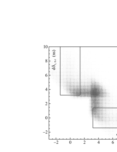
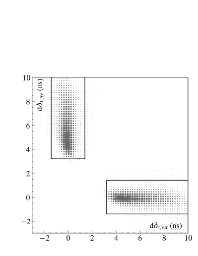
Figure 1: Scatter plot of the time differences $\mathrm{d}\delta_{t,\pi e}$ vs $\mathrm{d}\delta_{t,e\pi}$ for Monte Carlo events, for all $K_{S}$ decays (left) and for $K_{S}\rightarrow\pi e\nu$ decays (right).

After these TOF requirements, particle types and charges for signal events can be assigned very precisely: the probability of misidentifying a $\pi^{+}e^{-}\bar{\nu}$ event as $\pi^{-}e^{+}\nu$ or vice versa is negligible. These cuts reject $\sim\!90\%$ of the background events, while the efficiency for the signal is $\sim\!85\%$.

Once particle identification has been performed, we reevaluate the time differences $\delta_{t}(m)$, this time using for each track the mass assignment known from the cut on $d\delta_{t,e\pi}$ and subtracting the $T_{0}$ of the event. For the $T_{0}$ determination, the bunch crossing producing the event is evaluated as the integer part of the ratio $[\delta_{t}(e)+\delta_{t}(\pi)]/2T_{\mathrm{bunch}}$. We apply another TOF cut by selecting the events within the circle in the $\delta_{t}(e)$-$\delta_{t}(\pi)$ plane, as shown in Fig. 2 for MC events. This cut improves the background rejection by a factor of five, while eliminating 8% of the signal events at this analysis stage.

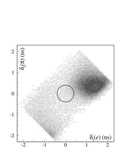
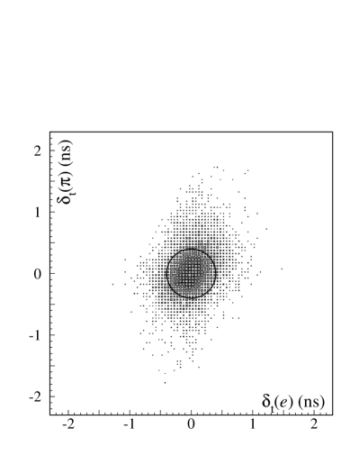
Figure 2: Scatter plot of the time differences $\delta_{t}(\pi)$ vs $\delta_{t}(e)$ for $\pi$ and $e$ mass assignments for Monte Carlo events, for all $K_{S}$ decays (left) and for $K_{S}\rightarrow\pi e\nu$ decays (right). Events within the circles are retained.

A powerful discriminating variable is the difference between the missing energy and momentum, $\Delta E_{\pi e}\!=\!E_{\mathrm{miss}}-p_{\mathrm{miss}}$, which is evaluated using the $K_{S}$ momentum known from the $K_{L}$ direction. For $\pi e\nu$ decays, $E_{\mathrm{miss}}$ and $p_{\mathrm{miss}}$ are the neutrino energy and momentum, and are equal. The distribution of $\Delta E_{\pi e}$ is shown in Fig. 3 after TOF cuts are imposed for $\pi^{-}e^{+}\nu$ (left panel) and for $\pi^{+}e^{-}\bar{\nu}$ (right panel) candidate events. A clear peak around zero is evident and corresponds to a clean signal for $K_{S}\rightarrow\pi e\nu$.

The residual background is dominated by $K_{S}\rightarrow\pi^{+}\pi^{-}(\gamma)$ decays. Events with $\Delta E_{\pi e}\!>\!10$ MeV are mostly due to cases in which one pion decays to a muon before entering the tracking volume (“$\pi\mu$” events), in which the track identified as electron by TOF is badly reconstructed (“$\pi_{\mathrm{bad}}\pi$” events), or in which the radiated photon has an energy in the $K_{S}$ frame above 7 MeV, thus shifting $M_{\pi\pi}$ below 490 MeV and $E_{\mathrm{miss}}$ toward positive values (“$\pi\pi\gamma$” events). Events with $\Delta E_{\pi e}\!<\!-10$ MeV are mostly “$\pi\mu$” or “$\pi_{\mathrm{bad}}\pi$” events, or are due to cases in which the track identified as the pion by TOF is badly reconstructed (“$\pi\pi_{\mathrm{bad}}$” events).

We discriminate between signal and residual background events by means of 5 kinematic variables: $\Delta E_{\pi e}$ itself; the difference $\mathrm{d}_{\mathrm{PCA}}$ between the impact parameters of the two tracks with the IP; the difference $\Delta E_{\pi\pi}$ in the $\pi$-$\pi$ hypothesis; the squared mass $M^{2}_{\mathrm{trk}}(e)$ of track 1(2) when it is identified as electron from TOF, calculated assuming that $p_{S}-p_{2(1)}$ is the momentum of an undetected pion and that $(p_{S}-p_{1}-p_{2})^{2}=0$; the energy $E^{*}_{\pi(e)}$ of the track identified as a $\pi$ ($e$) from TOF, calculated in the $K_{S}$ rest frame using the pion mass hypothesis.

Except for “$\pi\pi\gamma$” events, all of the background categories are characterized by poor vertex reconstruction quality, leading to a broad distribution of $\mathrm{d}_{\mathrm{PCA}}$ as shown in Fig. 4, top left. In contrast, signal and “$\pi\pi\gamma$” events are peaked around zero. We discriminate “$\pi\mu$” events by the $M^{2}_{\mathrm{trk}}(e)$ variable, which peaks around $m_{\mu}^{2}$, and “$\pi\pi\gamma$” events by the $\Delta E_{\pi\pi}$ variable, which peaks around zero. Finally, well reconstructed pion tracks from $K_{S}\rightarrow\pi^{+}\pi^{-}$ decays are identified by the value of $E^{*}$, which peaks around $m_{K}/2$, allowing us to recognize $\pi_{\mathrm{bad}}\pi$ or $\pi\pi_{\mathrm{bad}}$ events.

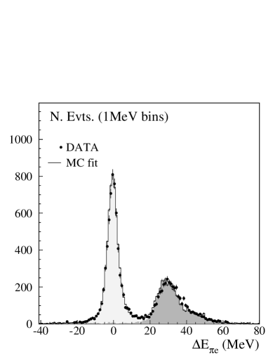
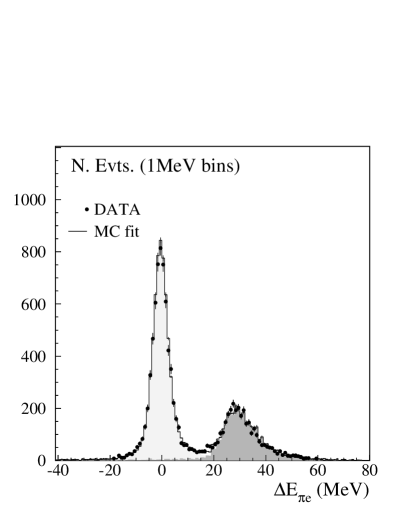
Figure 3: $E_{\mathrm{miss}}-p_{\mathrm{miss}}$ spectrum for events selected as $\pi^{-}e^{+}\nu$ (left panel) and $\pi^{+}e^{-}\bar{\nu}$ (right panel). Filled dots represent data from the entire data set; the solid line is the result of a fit varying the normalization of MC distributions for signal (light gray) and background (dark gray), which are also shown.

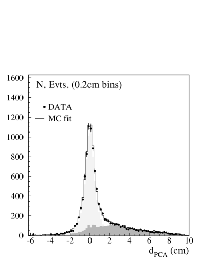
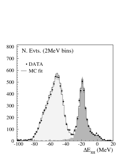
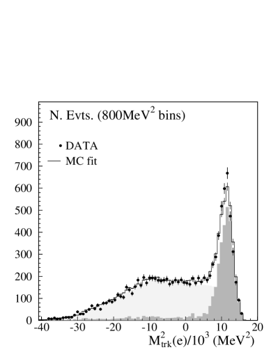
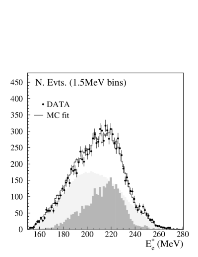
Figure 4: Distributions for $\pi^{+}e^{-}\bar{\nu}$ candidate events, for data (dots) and Monte Carlo events (solid line). Top left: $\mathrm{d}_{\mathrm{PCA}}$ variable, peaking around zero for vertices of good quality (signal and $\pi\pi\gamma$ events); top right: $\Delta E_{\pi\pi}$, peaking around zero for $\pi\pi\gamma$ events; bottom left: $M^{2}_{\mathrm{trk}}(e)$, peaking around $m_{\mu}^{2}$ for $\pi\mu$ events; bottom right: $E^{*}_{e}$, peaking around $m_{K}/2$ for $\pi\pi_{\mathrm{bad}}$ events. In each plot, signal (light gray) and background (dark gray) contributions are also shown.

The number of events due to signal and to each of the background categories are evaluated through a global binned-likelihood fit using the above variables. Each event is assigned to one of five regions in the $\Delta E_{\pi e}$-$\mathrm{d}_{\mathrm{PCA}}$ plane illustrated in Fig. 5. For each region, we use for the fit one of the variables defined above. The choice of the regions and the assignment of the fit variables to each region ensure good separation between each component in turn and all the others. In each region, the data are fit with the sum of the MC distributions in the appropriate variable for signal events and for events from each background source. The free parameters are the signal and background normalizations. For each source, the same normalization parameter is used in all fit regions.

Figure 5: Definition of the fit regions in the $\Delta E_{\pi e}$-$\mathrm{d}_{\mathrm{PCA}}$ plane. In each region, the variable used for the fit is also specified.

The result of the fit is shown as the solid line in the distributions of Figs. 3 and 4. The MC simulations of $K_{S}\rightarrow\pi e\nu$ and $K_{S}\rightarrow\pi^{+}\pi^{-}$ decays include photon radiation in the final state [15]. If the effect of radiation were not taken into account, the result for the branching ratio would decrease by a few percent.

We perform two independent fits, one for each charge state. The estimated numbers of signal events are shown in Tab. 1. The quoted statistical errors include the contributions from fluctuations in the signal statistics, from the background subtraction, and from the finite MC statistics [16].

The systematic errors include the contribution from uncertainty in the shape of the signal distributions. In particular, we have studied in detail the reliability of the MC in reproducing the distribution of $\Delta E_{\pi e}$. We have compared data and MC resolutions obtained from samples of $K_{S}\rightarrow\pi^{+}\pi^{-}$ events tagged by the $K_{L}$ crash, both for the momentum of each track and for the $\Delta E_{\pi\pi}$ variable. From these studies, we have extracted corrections to the MC resolutions for the tracking momentum and the polar and azimuthal angles for the $K_{L}$ crash. After these corrections are applied, good agreement is observed for the core of the $\Delta E_{\pi e}$ distribution for signal events. In order to study the reliability of the simulation for the tails, an additional variable $x_{\mathrm{PID}}$ has been used to discriminate signal events. $x_{\mathrm{PID}}$ identifies $e^{\pm}$ tracks on the basis of the spatial distribution of the energy deposition in the EmC, and is independent from the track momenta used to obtain the fit variables. An alternative estimate of the number of signal events in each fit region is obtained from the $x_{\mathrm{PID}}$ distribution, which is reliably reproduced by the MC simulation. Using this method, a significant difference in the number of signal events is observed only in regions 1 and 2, from which a shape correction is defined. This corresponds to a 0.5% correction to the final result, which is also taken as the corresponding systematic error.

The cut on the minimum cluster energy required for $K_{L}$-crash tagging dramatically affects the fraction of signal events in the tails of the $\Delta E_{\pi e}$ distribution: the looser the cut, the worse the resolution on the $K_{S}$ momentum evaluated from the $K_{L}$ direction. In order to check the robustness of the signal extraction, we have compared results obtained using three values for the minimum $K_{L}$ cluster energy: 125 MeV, 200 MeV, and 300 MeV. The results obtained using independent samples are compatible with each other. The intermediate cut gives the minimum total uncertainty.

A detailed description of the fit procedure is given in Ref. 9.

4 Efficiency estimates

For both $K_{S}\rightarrow\pi^{+}\pi^{-}$ (normalization) and $K_{S}\rightarrow\pi e\nu$ (signal) events, we estimate the corrections for the geometrical acceptance and tagging and selection inefficiencies with the MC simulation. In order to account for data-MC differences, we weight each event with the ratio of the data and MC tracking efficiencies extracted from various control samples. We evaluate the probabilities for finding EmC clusters from $K_{S}$ daughter particles and for satisfying the trigger conditions by combining data-extracted efficiencies, parametrized in terms of track momenta, with MC kinematics. For $K_{S}\rightarrow\pi e\nu$ events, we also use prompt $K_{L}\rightarrow\pi e\nu$ decays tagged by $K_{S}\rightarrow\pi^{+}\pi^{-}$ as a data control sample for efficiency evaluation. With this method, we obtain alternative estimates for the trigger and cluster efficiencies and evaluate the corrections for vertex reconstruction and $\pi$-$e$ TOF identification inefficiencies. These methods are described in detail in Refs. 9 and 17.

For $K_{S}\rightarrow\pi e\nu$ decays, the efficiencies are determined separately for each charge state and for the 2001 and 2002 data. We summarize the results for the overall efficiencies, given the tag requirement, in Tab. 2. The differences between the efficiencies for the two charge states arise from the different response of the calorimeter to $\pi^{+}$ and $\pi^{-}$, influencing the cluster, trigger, and TOF efficiencies. The uncertainties on the tracking and cluster/trigger efficiencies contribute approximately equally to the systematic errors on the overall efficiencies. A variation in the cluster/trigger efficiencies between 2001 and 2002 is reflected in the values for the overall efficiencies. The corresponding systematic errors have been estimated from the comparison of the results obtained using prompt $K_{L}\rightarrow\pi e\nu$ decays and using single-particle weights to correct the MC. The difference between the results obtained with the two methods is larger for $\pi^{-}e^{+}\nu$ events, and for the 2002 data.

$K_{S}$ decay	Selection efficiency
	Year 2001	Year 2002
$\pi^{+}\pi^{-}$	$0.5954\pm 0.0004_{\mbox{stat}}\pm 0.0010_{\mbox{syst}}$	$0.6035\pm 0.0004_{\mbox{stat}}\pm 0.0010_{\mbox{syst}}$
$\pi^{-}e^{+}\nu$	$0.2139\pm 0.0019_{\mbox{stat}}\pm 0.0014_{\mbox{syst}}$	$0.2197\pm 0.0012_{\mbox{stat}}\pm 0.0021_{\mbox{syst}}$
$\pi^{+}e^{-}\bar{\nu}$	$0.2252\pm 0.0016_{\mbox{stat}}\pm 0.0009_{\mbox{syst}}$	$0.2328\pm 0.0011_{\mbox{stat}}\pm 0.0011_{\mbox{syst}}$

Table 2: Selection efficiencies for $K_{S}\rightarrow\pi^{+}\pi^{-}$ and $K_{S}\rightarrow\pi e\nu$ decays, for the 2001 and 2002 data sets, given the $K_{L}$-crash tag.

In principle, the $K_{L}$-crash identification efficiency cancels out in the ratio of the number of selected $K_{S}\rightarrow\pi e\nu$ and $K_{S}\rightarrow\pi^{+}\pi^{-}$ events. In practice, since the event $T_{0}$ is obtained from the $K_{S}$ and the $K_{L}$ is recognized by its time of flight, there is a small dependence of the $K_{L}$-crash identification efficiency on the $K_{S}$ decay mode. A correction for this effect is obtained by studying the accuracy of the $T_{0}$ determination in each case [9, 18, 17]. The ratio $R_{\mathrm{tag}}$ of the tagging efficiencies for $K_{S}\rightarrow\pi e\nu$ and $K_{S}\rightarrow\pi^{+}\pi^{-}$ is found to differ from unity by $\sim\!1\%$. This effect is included in the efficiency values shown in Tab. 2.

5 Results

For each charge state and for the data set for each year, we obtain the ratio of BR’s by normalizing the number of signal events to the number of $K_{S}\rightarrow\pi^{+}\pi^{-}$ events and correcting for the overall selection efficiencies:

$$\frac{\Gamma(\mbox{$K_{S}$}\rightarrow\pi^{\mp}e^{\pm}\nu(\overline{\nu}))}{\Gamma(K_{S}\rightarrow\pi^{+}\pi^{-})}=\frac{N(\pi^{\mp}e^{\pm}\nu(\overline{\nu}))}{N(\pi\pi)}\times\frac{\epsilon_{\mathrm{tot}}^{\pi\pi}}{\epsilon_{\mathrm{tot}}^{\pm}}.$$

The results for the BR’s from the data sets for each year are compatible with probabilities greater than 50%. Averaging the results obtained for each data set, we obtain the following results:

  $${R_{e+}\equiv\frac{\Gamma(\mbox{$K_{S}$}\rightarrow\pi^{-}e^{+}\nu)}{\Gamma(K_{S}\rightarrow\pi^{+}\pi^{-})}} {{}=(5.099\pm 0.082_{\rm stat}\pm 0.039_{\rm syst})\times 10^{-4}} {R_{e-}\equiv\frac{\Gamma(\mbox{$K_{S}$}\rightarrow\pi^{+}e^{-}\bar{\nu})}{\Gamma(K_{S}\rightarrow\pi^{+}\pi^{-})}} {{}=(5.083\pm 0.073_{\rm stat}\pm 0.042_{\rm syst})\times 10^{-4}} {R_{e}\equiv\frac{\Gamma(\mbox{$K_{S}$}\rightarrow\pi e\nu)}{\Gamma(K_{S}\rightarrow\pi^{+}\pi^{-})}} {{}=(10.19\pm 0.11_{\rm stat}\pm 0.07_{\rm syst})\times 10^{-4}}$$   (6)

To obtain the value of the ratio $\mathrm{BR}(\mbox{$K_{S}$}\rightarrow\pi e\nu)/\mathrm{BR}(K_{S}\rightarrow\pi^{+}\pi^{-})$ we take into account the correlation between the values measured for the two charge modes. This correlation arises from uncertainties on the shapes of the signal distributions in the fit variables that are common to both charge states; the correlation parameter is 13%.

The charge asymmetry of Eq. (1) is given by:

$$A_{S}\!=\!\frac{N(\pi^{-}e^{+}\nu)/\epsilon_{\mathrm{tot}}^{+}-N(\pi^{+}e^{-}\bar{\nu})/\epsilon_{\mathrm{tot}}^{-}}{N(\pi^{-}e^{+}\nu)/\epsilon_{\mathrm{tot}}^{+}+N(\pi^{+}e^{-}\bar{\nu})/\epsilon_{\mathrm{tot}}^{-}}.$$

Combining the results for all data, we obtain:

$$A_{S}\!=\!(1.5\pm 9.6_{\mathrm{stat}}\pm 2.9_{\mathrm{syst}})\times 10^{-3}.$$

In order to perform a stability test, we have divided the entire data set into 17 samples and performed the analysis individually for each sample. Values of $\chi^{2}$ corresponding to probabilities above 50% are observed for all of the measured quantities [9].

The various contributions to the total fractional error on $\mathrm{BR}(K_{S}\rightarrow\pi e\nu)$ and to the total error on $A_{S}$ are listed in Tabs. 3 and 4. For the measurement of the BR, the uncertainty on the signal count from fit systematics is the dominant contribution to the total systematic error.

	Fractional error ($10^{-3}$)
	Statistical	Systematic
Statistics of $K_{S}\rightarrow\pi e\nu$	9.1
Statistics of $K_{S}\rightarrow\pi^{+}\pi^{-}$	0.1
Preselection efficiency, $K_{S}\rightarrow\pi e\nu$	1.5	2.9
Trigger efficiency, $K_{S}\rightarrow\pi e\nu$	0.2	0.3
TOF efficiency, $K_{S}\rightarrow\pi e\nu$	2.3
Fit systematics, $K_{S}\rightarrow\pi e\nu$		6.2
Preselection efficiency, $K_{S}\rightarrow\pi^{+}\pi^{-}$	0.3	1.6
Trigger efficiency, $K_{S}\rightarrow\pi^{+}\pi^{-}$	0.1	0.8
Ratio of tagging efficiencies	5.0
Ratio of cosmic veto inefficiencies	1.0
Total	10.8	7.1
Total fractional error	12.9

Table 3: Contributions to the fractional error on $\mathrm{BR}(K_{S}\rightarrow\pi e\nu)/\mathrm{BR}(K_{S}\rightarrow\pi^{+}\pi^{-})$.

	Error ($10^{-3}$)
	Statistical	Systematic
Statistics of $K_{S}\rightarrow\pi e\nu$	9.1
Preselection efficiency, $K_{S}\rightarrow\pi e\nu$	1.5	2.9
Trigger efficiency, $K_{S}\rightarrow\pi e\nu$	0.1	0.3
TOF efficiency, $K_{S}\rightarrow\pi e\nu$	2.3
Fit systematics, $K_{S}\rightarrow\pi e\nu$		0.4
Tagging efficiencies	0.4
Cosmic veto inefficiencies	1.0
Total	9.6	2.9
Total error	10.0

Table 4: Contributions to the absolute error on $A_{S}$.

For the purposes of measuring the dependence of the form factor $f_{+}(t)/f_{+}(0)$ on the 4-momentum transfer squared $t=(P_{K}-P_{\pi})^{2}$, the elimination of background from the sample while preserving statistics is a more important consideration than the understanding of the selection efficiencies at the level required in the branching-ratio analysis. We therefore use slightly different selection criteria to isolate a clean sample of $K_{S}\rightarrow\pi e\nu$ events: we require $|\Delta E_{\pi e}|\!<\!10{\rm\,M{e\kern-0.70007ptV}}$ and cut on the quality of the $K_{S}$ vertex. In order to limit loss of statistics, we loosen the energy requirement on the $K_{L}$ crash to 125 MeV. We select about 15 000 signal events, combining the data for the two years and charge modes. With this selection, the bacgkround contamination is reduced to 0.7%. Because of the limited statistics, we only measure the slope parameter of the form factor in the linear approximation, $f_{+}(t)/f_{+}(0)=1+\lambda_{+}t/m_{\pi}^{2}.$ More precisely, we fit the ratio of data and MC distributions in $t/m_{\pi+}^{2}$ with the function:

$$F(t)=A\times\left(\frac{1+\lambda_{+}t/m_{\pi+}^{2}}{1+\lambda_{+,MC}t/m_{\pi+}^{2}}\right)^{2},$$

where $A$ and $\lambda_{+}$ are the free parameters of the fit, and $\lambda_{+,MC}=0.03$ is the value of the slope used in the MC generation. Effects from the finite resolution on $t$ are negligible with respect to the statistical error and are ignored. We find $\lambda_{+}=(33.9\pm 4.1)\times 10^{-3}$ with $\chi^{2}/\mathrm{dof}=12.9/11$, corresponding to a probability $P(\chi^{2})\simeq 30\%$. This result is in reasonable agreement with the value of $\lambda_{+}$ for semileptonic $K_{L}$ and $K^{+}$ decays, $(28.82\pm 0.34)\times 10^{-3}$, from the average of results from KTeV [19], ISTRA+ [20], NA48 [21], and KLOE. [22].

6 Interpretation of the results

6.1 Determination of absolute BR’s

In order to evaluate the BR’s for the semileptonic modes, we combine the ratios of BR’s measured for each charge [Eq. (6)] with the most precise measurement of the ratio

$$R=\frac{\Gamma(K_{S}\rightarrow\pi^{+}\pi^{-})}{\Gamma(K_{S}\rightarrow\pi^{0}\pi^{0})}=2.236\pm 0.015,$$ (7)

which was also obtained at KLOE [23]. The only remaining mode with a BR large enough to measurably affect the constraint $\sum_{f}\mathrm{BR}(\mbox{$K_{S}$}\!\rightarrow\!f)\!=\!1$ is $K_{\mu 3}$; the BR’s for all other channels sum up to $\sim 10^{-5}$. Assuming lepton universality, we have

$$r_{\mu e}=\frac{\Gamma\left(K_{S}\rightarrow\pi\mu\nu\right)}{\Gamma\left(K_{S}\rightarrow\pi e\nu\right)}=\frac{1+\delta_{K}^{\mu}}{1+\delta_{K}^{e}}\frac{I_{K}^{\mu}}{I_{K}^{e}},$$ (8)

where $\delta_{K}^{\mu,e}$ are mode-dependent long-distance radiative corrections and $I_{K}^{\mu,e}$ are decay phase-space integrals. Using $I_{K}^{\mu}/I_{K}^{e}=0.6622(18)$ from KTeV [24] and $(1+\delta_{K}^{\mu})/(1+\delta_{K}^{e})=1.0058(10)$ from Ref. 25, we get $r_{\mu e}=0.6660(19)$. We evaluate the four main BR’s of the $K_{S}$ from

$$\mathrm{BR}(\mbox{$K_{S}$}\to i)=\frac{\Gamma(\mbox{$K_{S}$}\to i)/\Gamma(K_{S}\rightarrow\pi^{+}\pi^{-})}{1+1/R+(R_{e+}+R_{e-})(1+r_{\mu e})},$$ (9)

where $i\!=\!\pi^{+}\pi^{-},\,\pi^{0}\pi^{0},\,\pi^{-}e^{+}\nu,\,\pi^{+}e^{-}\bar{\nu}$. We find:

  $${\mathrm{BR}(K_{S}\rightarrow\pi^{+}\pi^{-})} {{}=(69.02\pm 0.14)\times 10^{-2}} {\mathrm{BR}(K_{S}\rightarrow\pi^{0}\pi^{0})} {{}=(30.87\pm 0.14)\times 10^{-2}} {\mathrm{BR}(K_{S}\rightarrow\pi^{-}e^{+}\nu)} {{}=(3.519\pm 0.063)\times 10^{-4}} {\mathrm{BR}(K_{S}\rightarrow\pi^{+}e^{-}\bar{\nu})} {{}=(3.508\pm 0.058)\times 10^{-4}}$$   (10)

The correlation matrix $\langle\delta_{i}\delta_{j}\rangle/\sqrt{\langle\delta_{i}^{2}\rangle\langle\delta_{j}^{2}\rangle}$ is:

$$\begin{array}[]{cc}&\begin{array}[]{cccc}\pi^{+}\pi^{-}\kern 8.53581pt&\pi^{0}\pi^{0}\kern 8.53581pt&\kern 2.84526pt\pi^{-}e^{+}\nu\kern 5.69054pt&\kern 2.84526pt\pi^{+}e^{-}\overline{\nu}\kern 2.84526pt\\ \end{array}\\ \begin{array}[]{c}\pi^{+}\pi^{-}\\ \pi^{0}\pi^{0}\\ \pi^{-}e^{+}\nu\\ \pi^{+}e^{-}\overline{\nu}\\ \end{array}&\left(\begin{array}[]{cccc}1&-0.9999&0.1106&0.1196\\ -0.9999&1&-0.1187&-0.1272\\ 0.1106&-0.1187&1&0.1445\\ 0.1196&-0.1272&0.1445&1\\ \end{array}\right)\end{array}$$ (11)

The contribution from the error on $r_{\mu e}$ is included in the systematic errors. Taking correlations into account, we have:

$$\mathrm{BR}(K_{S}\rightarrow\pi e\nu)=\left(7.028\pm 0.092\right)\times 10^{-4}.$$ (12)

6.2 Test of the $\Delta S=\Delta Q$ rule

From the total BR we test the validity of the $\Delta S=\Delta Q$ rule in $CPT$-conserving transitions [Eq. (4)]. We use the following values for the $K_{S}$ and $K_{L}$ lifetimes: $\tau_{S}=0.08958(6)$ ns from the PDG [13] and $\tau_{L}=50.84(23)$ ns from recent measurements from KLOE [26, 27]. For $\mathrm{BR}(K_{L}\rightarrow\pi e\nu)$, we use the value from KLOE, 0.4007(15) [26]. We obtain:

$$\mathrm{Re}\,x_{+}=\left(-1.2\pm 3.6\right)\times 10^{-3}.$$ (13)

The error on this value represents an improvement by almost a factor of two with respect to the most precise previous measurement, that from the CPLEAR experiment [5].

6.3 Test of the $CPT$ symmetry

From the sum and difference of the $K_{L}$ and $K_{S}$ charge asymmetries one can test for possible violations of the $CPT$ symmetry, either in the decay amplitudes or in the mass matrix [Eqs. (2) and (3)]. Using $A_{L}=(3.34\pm 0.07)\times 10^{-3}$ [13], we obtain from Eq. (2)

$$\mathrm{Re}\,x_{-}+\mathrm{Re}\,\delta=\left(-0.5\pm 2.5\right)\times 10^{-3}.$$ (14)

Current knowledge of these two parameters is dominated by results from CPLEAR [3]: the error on $\mathrm{Re}\,\delta$ is $3\times 10^{-4}$ and that on $\mathrm{Re}\,x_{-}$ is $10^{-2}$. Using $\mathrm{Re}\,\delta=(3.0\pm 3.3_{\rm stat}\pm 0.6_{\rm syst})\times 10^{-4}$ from CPLEAR, we obtain:

$$\mathrm{Re}\,x_{-}=\left(-0.8\pm 2.5\right)\times 10^{-3},$$ (15)

thus improving on the error of $\mathrm{Re}\,x_{-}$ by a factor of five.

From Eq. (3) we obtain

$$\mathrm{Re}\,\epsilon-\mathrm{Re}\,y=\left(1.2\pm 2.5\right)\times 10^{-3}.$$ (16)

We calculate $\mathrm{Re}\,\epsilon$ using values from Ref. 13 that are obtained without assuming $CPT$ conservation: $\mathrm{Re}\,\epsilon=|\epsilon|\times\cos{\phi_{\epsilon}}=(1.62\pm 0.04)\times 10^{-3}$. Subtracting this value from Eq. (16), we find

$$\mathrm{Re}\,y=\left(0.4\pm 2.5\right)\times 10^{-3},$$ (17)

which has precision comparable to that ($3\!\times\!10^{-3}$) obtained from the unitarity relation by CPLEAR [4].

6.4 Determination of $V_{us}$

The value of $V_{us}$ can be extracted from the measurement of $\mathrm{BR}(\mbox{$K_{S}$}\rightarrow\pi e\nu)$ and from the $K_{S}$ lifetime, $\tau_{S}$:

$$V_{us}\ \times f_{+}^{K^{0}\pi^{-}}(0)=\left[\frac{128\,\pi^{3}\,\mathrm{BR}(\mbox{$K_{S}$}\rightarrow\pi e\nu)}{\tau_{S}\,G_{\mu}^{2}\,M_{K}^{5}\,S_{\mathrm{ew}}\,I_{K}(\lambda_{+},0)}\right]^{1/2}\frac{1}{1+\delta^{K}_{{\mathrm{em}}}},$$ (18)

where $f_{+}^{K^{0}\pi^{-}}(0)$ is the vector form factor at zero momentum transfer and $I_{K}(\lambda_{+},0)$ is the result of the phase space integration after factoring out $f_{+}^{K^{0}\pi^{-}}(0)$; both quantities are evaluated in absence of radiative corrections. The radiative corrections [28, 25] for the form factor and the phase-space integral are included via the parameter $\delta^{K}_{{\mathrm{em}}}=(0.55\pm 0.10)\!\times\!10^{-2}$ [28]. The short-distance electroweak corrections are included in the parameter $S_{\mathrm{ew}}=1.0232$ [29].

The pole parametrization of the vector form factor is $f_{+}(t)=f_{+}(0)[M_{V}^{2}/(M_{V}^{2}-t)]$. Expanding this expression to second order gives $\lambda_{+}^{\prime\prime}=2\lambda_{+}^{\prime 2}$, where $\lambda_{+}^{\prime}$ and $\lambda_{+}^{\prime\prime}$ are the linear and quadratic slopes,

$$f_{+}(t)=f_{+}(0)\left[1+\lambda_{+}^{\prime}\frac{t}{m^{2}_{\pi^{+}}}+\frac{\lambda^{\prime\prime}_{+}}{2}\frac{t^{2}}{m^{4}_{\pi^{+}}}\right].$$

We evaluate the phase space integral from the value of $M_{V}$ from KLOE, $M_{V}\!=\!870.0\pm 9.2$ MeV [22], and get $I_{K}\!=\!0.10320\pm 0.00020$. The pole fit result is less affected by the strong correlation between the linear and quadratic slopes and provides better consistency among the values of $I_{K}$ from different experiments (KLOE [22], KTeV [19], ISTRA+ [20, 30], and NA48 [21]) than is obtained using the results for $\lambda_{+}^{\prime}$ and $\lambda_{+}^{\prime\prime}$.

We obtain:

$$f_{+}^{K^{0}\pi^{-}}(0)\times V_{us}\ =0.2150\pm 0.0014$$ (19)

Using $f_{+}^{K^{0}\pi^{-}}(0)=0.961\pm 0.008$ from Ref. 31 (this value is in agreement with a recent lattice calculation [32]), we get

$$V_{us}\!=\!0.2238\pm 0.0024.$$ (20)

To perform a test of first-row CKM unitarity, we define:

$$\Delta=1-V_{ud}^{2}-V_{us}^{2}-V_{ub}^{2}$$

Using $V_{ud}\!=\!0.97377\pm 0.00027$ from Ref. 33 and including the small contribution of $V_{ub}$ [13], we obtain

$$\Delta=\left(1.7\pm 1.2\right)\times 10^{-3},$$ (21)

which is compatible (1.4 $\sigma$) with zero.

A new measurement of $R$ has recently been made at KLOE, with a precision improved by more than a factor of two with respect to Eq. 7. Combining the new and old KLOE measurements, we obtain $R\!=2.2549\pm 0.0054$. The results presented in Eqs. 10, 12, 13, 19, 20, and 21 depend only slightly on the value used for $R$. The results obtained using the updated value of $R$ are listed below:

  $${\mathrm{BR}(K_{S}\rightarrow\pi^{+}\pi^{-})} {{}=(69.196\pm 0.051)\times 10^{-2}} {\mathrm{BR}(K_{S}\rightarrow\pi^{0}\pi^{0})} {{}=(30.687\pm 0.051)\times 10^{-2}} {\mathrm{BR}(K_{S}\rightarrow\pi^{-}e^{+}\nu)} {{}=(3.528\pm 0.062)\times 10^{-4}} {\mathrm{BR}(K_{S}\rightarrow\pi^{+}e^{-}\bar{\nu})} {{}=(3.517\pm 0.058)\times 10^{-4}} {\mathrm{BR}(K_{S}\rightarrow\pi e\nu)} {{}=(7.046\pm 0.091)\times 10^{-4}}$$   (22)

From the last of these, the following quantities follow:

  $${\mathrm{Re}\,x_{+}} {{}=(-0.5\pm 3.6)\times 10^{-3}} {f_{+}^{K^{0}\pi^{-}}(0)\times V_{us}\ } {{}=0.2153\pm 0.0014} {V_{us}} {{}=0.2240\pm 0.0024} {\Delta} {{}=(1.6\pm 1.2)\times 10^{-3}}$$   (23)

The differences between these quantities when calculated using the old and new values of $R$ are well within the stated uncertainties.

References

• [1] M. Ademollo, R. Gatto, Phys. Rev. Lett. 13 (1964) 264.
• [2] KTeV Collaboration, A. Alavi-Harati et al., Phys. Rev. Lett. 88 (2002) 181601.
• [3] CPLEAR Collaboration, A. Angelopoulos, et al., Phys. Lett. B444 (1998) 52.
• [4] CPLEAR Collaboration, A. Apostolakis, et al., Phys. Lett. B456 (1999) 297.
• [5] CPLEAR Collaboration, A. Angelopoulos, et al., Phys. Lett. B444 (1998) 38.
• [6] KLOE Collaboration, A. Aloisio, et al., Phys. Lett. B535 (2002) 37.
• [7] KLOE Collaboration, M. Adinolfi, et al., Nucl. Instr. and Meth. A488 (2002) 51.
• [8] KLOE Collaboration, M. Adinolfi, et al., Nucl. Instr. and Meth. A482 (2002) 363.
• [9] C. Gatti, T. Spadaro, KLOE Note 208 (2006), unpublished.
URL http://www.lnf.infn.it/kloe/pub/knote/kn208.ps
• [10] KLOE Collaboration, M. Adinolfi, et al., Nucl. Instr. and Meth. A492 (2002) 134.
• [11] N. Paver, Riazuddin, Phys. Lett. B246 (1990) 240.
• [12] N. Brown, F. E. Close, Scalar mesons and kaons in $\phi$ radiative decay & their implications for studies of CP violation at DAΦNE, in: L. Maiani, G. Pancheri, N. Paver (Eds.), The DAΦNE Physics Handbook, Vol. 2, 1992, p. 447.
• [13] S. Eidelman, et al., Particle Data Group, Phys. Lett. B592, and 2005 partial update for edition 2006.
URL http://pdg.lbl.gov
• [14] KLOE Collaboration, F. Ambrosino, et al., Precise measurement of $\Gamma(K_{S}\rightarrow\pi^{+}\pi^{-})/\Gamma(K_{S}\rightarrow\pi^{0}\pi^{0})$ with the KLOE detector at DAΦNE, hep-ex/0601025.
• [15] C. Gatti, Eur. Phys. J. C45 (2005) 417, and references therein.
• [16] R. J. Barlow, C. Beeston, Comput. Phys. Commun. 77 (1993) 219.
• [17] C. Gatti, T. Spadaro, KLOE Note 176 (2002), unpublished.
URL http://www.lnf.infn.it/kloe/pub/knote/kn176.ps.gz
• [18] C. Gatti, M. Palutan, T. Spadaro, KLOE Note 209 (2006), unpublished.
URL http://www.lnf.infn.it/kloe/pub/knote/kn209.ps
• [19] KTeV Collaboration, T. Alexopoulos, et al., Phys. Rev. D70 (2004) 092007.
• [20] O. P. Yushchenko, et al., Phys. Lett. B589 (2004) 111.
• [21] NA48 Collaboration, A. Lai, et al., Phys. Lett. B604 (2004) 1.
• [22] KLOE Collaboration, F. Ambrosino, et al., Measurement of the form-factor slopes for the decay $K_{L}\rightarrow\pi e\nu$ with the KLOE detector hep-ex/0601038, accepted for publication by Phys. Lett. B.
• [23] KLOE Collaboration, A. Aloisio et al., Phys. Lett. B538 (2002) 21.
• [24] KTeV Collaboration, T. Alexopoulos, et al., Phys. Rev. D70 (2004) 092007.
• [25] T. C. Andre, Radiative corrections to K0(l3) decays, hep-ph/0406006.
• [26] KLOE Collaboration, F. Ambrosino, et al., Phys. Lett. B632 (2006) 43.
• [27] KLOE Collaboration, F. Ambrosino, et al., Phys. Lett. B626 (2005) 15.
• [28] V. Cirigliano, H. Neufeld, H. Pichl, Eur. Phys. J. C35 (2004) 53.
• [29] W. J. Marciano, A. Sirlin, Phys. Rev. Lett. 71 (1993) 3629.
• [30] O. P. Yushchenko, et al., Phys. Lett. B581 (2004) 31.
• [31] H. Leutwyler, M. Roos, Z. Phys. C25 (1984) 91.
• [32] D. Becirevic, et al., Nucl. Phys. B705 (2005) 339.
• [33] W. J. Marciano, A. Sirlin, Phys. Rev. Lett. 96 (2006) 032002.