Abstract

We present a quantitative study on sensitivities to the top-decay anomalous couplings, taking into account realistic experimental conditions expected at Tevatron and LHC. A double angular distribution of $W$ and charged lepton in the top decay is analyzed, using $t\bar{t}$ events in the $lepton+jets$ channel. In order to improve sensitivities to the anomalous couplings, we apply two techniques: (1) We use a likelihood fitting method for full kinematical reconstruction of each top event. (2) We develop a new effective spin reconstruction method for leptonically-decayed top quarks; this method does not require spin information of the antitop side. For simplicity, we neglect couplings of right-handed bottom quark as well as $CP$ violating couplings. The 95% C.L. estimated bound on a ratio of anomalous couplings reads $-0.81<f_{2}/f_{1}<-0.70$, $-0.12<f_{2}/f_{1}<0.14$ using 1000 reconstructed top events at Tevatron, while $-0.74<f_{2}/f_{1}<-0.72$, $-0.01<f_{2}/f_{1}<0.01$ is expected with 100k reconstructed top events at LHC, where only statistical errors are taken into account. A two-fold ambiguity in the allowed range remains when the number of events exceeds a few hundred.

1 Introduction

The top quark is the heaviest elementary particle discovered up to now. Namely, the top quark mass term breaks the electroweak gauge symmetry maximally among all of the observed interactions of elementary particles. For this reason, we expect that the top quark can be used as a probe to search into the symmetry-breaking physics. On the other hand, so far reported experimental data from Tevatron on top quark properties are still limited; see e.g. [2, 3, 4]. No sign of significant deviations from the Standard Model (SM) predictions has been seen.

The number of observed top quark events in the Tevatron Run II experiment is increasing steadily and now reaching of the order of a few hundred. Moreover, it is expected that at LHC experiment an immense number of top quarks will be produced. Thus, we foresee that detailed properties of the top quark will start to be uncovered in near future.

Among various interactions of the top quark, study of the top quark decay properties is particularly interesting. In the SM (and many of its extensions), the top quark decays via electroweak interaction before hadronization. Hence, the top quark’s spin information is transferred directly to its decay daughters, and their distributions can be predicted reliably using perturbative calculations. Thus, the top quark spin can be used as a powerful analysis tool for scrutinizing top quark interactions.

There have been many theoretical studies on how to test top quark decay properties at hadron colliders. Non-standard effects on the total top decay width and on the top decay branching fractions to polarized $W$ states have been computed in the minimal-supersymmetric standard model [8, 9], in a $R$-parity violating supersymmetric model [10], and in the top-color assisted technicolor model [11]. A study was given on how to extract anomalous $tbW$ couplings and discriminate different underlying models from combined measurements of the top decay branching fractions to polarized $W$s and the single top production rates [12]. The top quark decay $t\to bW$ was studied within the non-commutative standard model in [13]. The correlation between $t$ and $\bar{t}$ spins in the $t\bar{t}$ events has been studied as a mean to investigate decay properties of the top quark [14, 15, 16, 17, 18]. Effects of anomalous couplings on the lepton rapidity and transverse energy distribution were briefly discussed in [19]. There have also been a vast number of studies on top rare decays and non-standard decay channels; see [20] and references therein.

In this paper we focus on effects of the anomalous $tbW$ couplings to the distributions of $W$ and charged lepton in the decay of top quarks. We estimate sensitivities to (some of) these couplings expected at Tevatron and LHC, using Monte Carlo simulations which take into account realistic experimental conditions at these colliders. There have been no other quantitative studies, using top quark decays, on sensitivities to the top decay anomalous couplings at hadron colliders.

A sensitivity study of the anomalous couplings using the single top production process was given in [21]. Their estimated sensitivities to the anomalous couplings are rather low, due to existence of huge background cross sections for $Wb\bar{b}$ and $Wb\bar{b}+jets$ processes. The small signal-to-noise ratio leads to large statistical as well as systematic errors. In this connection, we note that due to lack of data statistics and difficulty in the background estimation, the single top production process has not yet been observed at Tevatron [22, 23]. As compared to their analysis, our analysis method using $t\bar{t}$ events in the $lepton+jets$ mode is cleaner and involves controlled and small backgrounds. Consequently, our method improves sensitivities to the anomalous couplings considerably as compared to the results of [21].

In our analysis, we assume that there are only anomalous $tbW$ couplings for the left-handed bottom quark and we neglect $CP$ violation. We impose these assumptions, for simplicity of our analysis, and also in view of the present bounds on the general $tbW$ couplings. This leaves only two independent real anomalous couplings, and our analysis is sensitive only to the ratio of these two couplings. See Sec. 2 for details.

In order to improve sensitivities to the anomalous couplings, we devise two techniques. (1) We use a likelihood fitting method for full kinematical reconstruction of each $t\bar{t}$ event. (2) We develop a new method for reconstructing an effective spin direction of the top quark. In particular, the new feature of the latter technique is that we do not need to reconstruct the spin of the antitop side in the $t\bar{t}$ events, i.e. we do not make use of the correlation between the top and antitop spins. In a separate paper, two of the present authors elucidate theoretical aspects of the effective spin reconstructed in this method [24].

As well known, top quarks produced at Tevatron and LHC are scarcely polarized. It is one of the major reasons why people have considered correlations between top spin and antitop spin in the $t\bar{t}$ production process [14, 15, 16, 17, 18]; with the help of this correlation, one can, in principle, reconstruct the information of the top quark spin, by looking into the information on the antitop side. Nevertheless, if we are to use events in the dilepton channel, the event statistics is rather low (especially at Tevatron), leading to disadvantages with regard to the sensitivity study. On the other hand, if we are to use events in the $lepton+jets$ channel (which has not been tried at Tevatron up to now), we suffer from large systematic uncertainties due to the complexity in the reconstruction of the spin of a hadronically-decayed top quark.

At first our claim may seem unreasonable, as one might argue that it is impossible to reconstruct the spin of an unpolarized top quark: Since an unpolarized state is rotationally invariant, there exists no reference direction appropriate for a spin direction. While this argument is correct on its own, we can still reconstruct an effective “spin direction” of a top quark, practically useful in the analysis of top decay, in the following sense. Unpolarized top quarks can be interpreted as an admixture, where one-half of them have their spins in $+\vec{n}$ direction and the other half have their spins in $-\vec{n}$ direction, for an arbitrary chosen unit vector $\vec{n}$. Then the directions of the decay products from the top quarks with $+\vec{n}$ spin are strongly correlated with the $+\vec{n}$ direction, provided the top decay interaction is close to the SM prediction. For instance, the charged leptons are emitted preferentially in $+\vec{n}$ direction in the rest frame of the top quark. The same is true for the top quarks with $-\vec{n}$ spin. Then it seems reasonable (at least intuitively) to project the direction of the lepton $\vec{n}_{l}$ onto the $\vec{n}$-axis and define an effective spin direction as ${\rm sign}(\vec{n}\!\cdot\!\vec{n}_{l})\times\vec{n}$, for each event. Indeed certain angular distributions of the top decay products with respect to this effective spin direction reproduce fairly well the corresponding angular distributions from a truly polarized top quark. This is the case even including anomalous couplings. It is in this sense that the effective spin direction is practically useful. That we can choose any axis $\vec{n}$, and that any choice is equivalent (if we ignore experimental environment), guarantee the rotational invariance of the unpolarized state of the top quark.

In Sec. 2 we present our theoretical setups, namely the definitions of the anomalous couplings and theoretical formulas for the decay angular distributions. In Sec. 3 we propose our method for reconstructing an effective top spin direction and discuss why it can be useful. The MC simulations used in our analysis are explained in Sec. 4. Sec. 5 demonstrates the kinematical reconstruction of $t\bar{t}$ events using our likelihood fitting method. Sensitivities to the anomalous couplings are estimated using the selected $t\bar{t}$ event samples in Sec. 6. Conclusions are given in Sec. 7. In Appendix we present the theoretical formula for the double angular distribution when we use the effective spin direction.

2 Anomalous couplings in top decay vertex

It is conventional to incorporate effects of physics beyond the SM in various form factors of the interactions among the known particles. The interactions of fermions and gauge boson, in general, can be expressed by six form factors with a particular energy scale at which new physics is opened. If we assume that $W$ boson is on-shell, the number of the form factors is reduced to four. Thus, the effective $Wtb$ vertex relevant to the top quark decay is expressed as [25]

$$\Gamma_{Wtb}^{\mu}=-\frac{g}{\sqrt{2}}V_{tb}\bar{u}(p_{b})\left[\gamma^{\mu}(f_{1}^{L}P_{L}+f_{1}^{R}P_{R})-\frac{i\sigma^{\mu\nu}k_{\nu}}{M_{W}}(f_{2}^{L}P_{L}+f_{2}^{R}P_{R})\right]u(p_{t})\quad,$$ (1)

where $V_{tb}$ is the CKM (Cabibbo-Kobayashi-Maskawa) matrix element [26], $P_{L,R}$ $=$ $(1\mp\gamma_{5})/2$ is the left-handed/right-handed projection operator, and $k$ is the momentum of $W$. We take the convention in which the energy scale is represented by $M_{W}$. The form factors $f_{1}^{L,R}$ and $f_{2}^{L,R}$ are in general complex. At tree-level of the SM, their values are $f_{1}^{L}=1$ and $f_{1}^{R}=f_{2}^{L}=f_{2}^{R}=0$. We will be concerned only with the top quark decay process $t\to bW$, where $Q^{2}$ value is fixed, therefore, we treat the form factors as constants (couplings) henceforth. The decay vertex for the antitop quark can be written similarly in a straightforward manner.

There are some (indirect) constraints to these couplings from measurements of the FCNC processes of rare $B$ decays, $b\rightarrow s\gamma$ and $b\rightarrow sl^{+}l^{-}$, and from the precision measurements at $Z$ pole [7]. These measurements support consistency with the SM predictions. Apart from a somewhat loose constraint for the $f_{2}^{L}$ parameter, the non-Standard $CP$-violating and right-handed bottom quark couplings are severely constrained. Taking this into account, and for simplicity of the analysis, we assume in the following that the interactions in Eq. (1) preserve $CP$ symmetry and also neglect the couplings of the right-handed bottom quark. Hence, Eq. (1) is reduced to

$$\Gamma_{Wtb}^{\mu}=-\frac{g}{\sqrt{2}}V_{tb}\bar{u}(p_{b})\left[\gamma^{\mu}f_{1}P_{L}-\frac{i\sigma^{\mu\nu}k_{\nu}}{M_{W}}f_{2}P_{R}\right]u(p_{t})\quad,$$ (2)

$$\bar{\Gamma}_{W\bar{t}\bar{b}}^{\mu}=-\frac{g}{\sqrt{2}}V_{tb}\bar{v}(p_{\bar{t}})\left[\gamma^{\mu}{f}_{1}P_{L}-\frac{i\sigma^{\mu\nu}k_{\nu}}{M_{W}}{f}_{2}P_{L}\right]v(p_{\bar{b}})\quad,$$ (3)

where

$$f_{1}\equiv f_{1}^{L}=\bar{f}_{1}^{L}\quad,\quad f_{2}\equiv f_{2}^{R}=\bar{f}_{2}^{L}\quad,$$ (4)

and both $f_{1}$ and $f_{2}$ are real. For definiteness, we have shown both the top and antitop decay vertices explicitly. As stated, we have simply neglected $f_{1}^{R}$($\bar{f}_{1}^{R}$) and $f_{2}^{L}$($\bar{f}_{2}^{R}$) terms. Nevertheless, even if they happen to be non-vanishing (but not large), their effects are expected to be suppressed, since they enter the cross section formulas quadratically in the limit $m_{b}\to 0$, as they do not interfere with the SM amplitude. Hence, our treatment would be justified for a first analysis.

In Fig. 1, we show the partial decay width for $t\to bW$ for different values of $f_{1}$ and $f_{2}$/$f_{1}$, where the tree-level SM corresponds to ($f_{1}$,$f_{2}$) = (1,0). Apart from the overall normalization proportional to $f_{1}^{\,2}$, the partial decay width is a quadratic function of $f_{2}$/$f_{1}$. One sees that the partial decay width is below 10 GeV in a wide region in the ($f_{1}$,$f_{2}$) parameter space. The current resolution of the reconstructed top-quark invariant mass distribution using jet events at Tevatron is order 40 GeV. It follows that a wide region in the parameter space ($f_{1}$,$f_{2}$) is still allowed under the constraint from the present top invariant mass measurement.

In principle, we can use the present measurement of $W$ helicities [4] for constraining $f_{2}/f_{1}$. No explicit analysis has been given so far, however. From a rough estimate, we conjecture that a range $|f_{2}/f_{1}|\hbox{ \raise 3.0pt\hbox to0.0pt{$<$}\raise-3.0pt\hbox{$\sim$} }0.3$ is (at least) scarcely constrained at the present status.

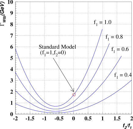
Figure 1: Tree-level partial width for $t\to bW$ as a function of $f_{2}/f_{1}$ and for different values of $f_{1}$. The unit is in GeV. The tree-level SM prediction corresponds to ($f_{1}$,$f_{2}$)=(1,0).

Let us discuss effects of the anomalous couplings, according to Eqs. (2) and (3), on the distribution of the decay products from the top quark. We may separate the dependences of the decay distribution on $f_{1}$ and on $f_{2}/f_{1}$. A variation of $f_{1}$ changes only the normalization of the (partial) decay width of the top quark, while a variation of $f_{2}/f_{1}$ changes both the normalization and the differential decay distributions. Since it is difficult to measure the absolute value of the decay width accurately in near future, our primary goal will be to measure (constrain) the value of $f_{2}/f_{1}$ from the measurement of the differential decay distribution. An efficient method was proposed in [27] using the decay process of the top quark at future $e^{+}e^{-}$ collider experiments. Noting that only the decay process is concerned, we can apply the main strategy of their method to our analysis aimed for hadron collider experiments. The relevant strategy is as follows. Since the transverse $W$ boson (denoted as $W_{T}$) is more sensitive to $f_{2}$ than the longitudinal $W$ boson ($W_{L}$), we can enhance the contribution of $W_{T}$ using the decay distribution. It is well known that the contribution of $W_{T}$ is dominant when $W$ is emitted opposite to the top spin direction in the decay $t\to bW$ and also when $l$ is emitted in the opposite direction to $W$ in the decay $W\to l\nu$. Hence, we can select these kinematical regions in order to enhance sensitivity to $f_{2}/f_{1}$.

The differential decay distribution of $W$ and $l$ in the semi-leptonic decay from a top quark with definite spin orientation is expressed as [25]

$$\frac{d\Gamma(t\rightarrow bW\!\rightarrow bl\nu)}{d\cos\theta_{W}d\cos\theta_{l}d\phi_{l}}=A{\left|(f_{2}+f_{1}\frac{M_{t}}{M_{W}})\cos\frac{\theta_{W}}{2}\sin\theta_{l}+(f_{1}+f_{2}\frac{M_{t}}{M_{W}})e^{-i\phi_{l}}\sin\frac{\theta_{W}}{2}(1-\cos\theta_{l})\right|}^{2},$$

(5)

with

$$A=\frac{3G_{F}|V_{tb}|^{2}M_{W}^{2}(M_{t}^{2}-M_{W}^{2})^{2}}{32\sqrt{2}\pi M_{t}^{3}}\times Br(W\rightarrow l\nu)\quad.$$ (6)

Here, $G_{F}$ is the Fermi constant. $\theta_{W}$ is defined as the angle between the top spin direction and the direction of $W$ in the top quark rest frame. $\theta_{l}$ is defined as the lepton helicity angle, which is the angle of the charged lepton in the rest frame of $W$ with respect to the original direction of the travel of $W$. $\phi_{l}$ is defined as the azimuthal angle of $l$ around the original direction of the travel of $W$. A schematic view of the angle definitions is shown in Fig. 2. The first term in the amplitude on the right-hand-side of Eq. (5) represents the contribution of $W_{L}$, while the second term represents the contribution of $W_{T}$.

After integrating over $\phi_{l}$, we obtain the double angular distribution

$$\frac{d\Gamma(t\rightarrow bW\!\rightarrow bl\nu)}{d\cos\theta_{W}d\cos\theta_{l}}=\pi\,A\,\biggl{[}\Bigl{(}f_{1}\frac{M_{t}}{M_{W}}+f_{2}\Bigr{)}^{2}\cos^{2}\frac{\theta_{W}}{2}\,\sin^{2}\theta_{l}$$

$$~{}~{}~{}~{}~{}~{}~{}~{}~{}~{}~{}~{}~{}~{}~{}~{}~{}~{}~{}~{}~{}~{}~{}~{}~{}~{}~{}~{}~{}~{}~{}~{}~{}~{}~{}~{}~{}~{}~{}~{}~{}+4\,\Bigl{(}f_{1}+f_{2}\frac{M_{t}}{M_{W}}\Bigr{)}^{2}\,\sin^{2}\frac{\theta_{W}}{2}\,\sin^{4}\frac{\theta_{l}}{2}\biggr{]}\,.$$ (7)

The one-loop QCD correction to the distribution Eq. (7) within the SM is known [28]. A large part of the correction goes to a variation of the normalization of the partial decay width, which amounts to about 9%, whereas the correction to the distribution shape (after the correction to the normalization is removed) is at the level of 1–2% or less. For simplicity, in most of the following discussion we discard the effect of the QCD correction; see also [24].

In Figs. 3, we show the normalized double angular distribution $N^{-1}d\Gamma(t\rightarrow bl\nu)/d\cos\theta_{W}d\cos\theta_{l}$; Fig. 3(a) corresponds to $(f_{1},f_{2})=(1,0)$ (tree-level SM) and (b) to $(f_{1},f_{2})=(1,0.3)$, respectively. Comparing the two figures, the effects of varying $f_{2}$ are indeed enhanced in the regions $\cos\theta_{W}\simeq-1$ and $\cos\theta_{l}\simeq-1$, in accord with enhancement of the $W_{T}$ contributions in these regions.

Thus, it is crucial to reconstruct the top quark’s spin orientation in this method. At hadron collider experiments, it is much more non-trivial to reconstruct the top quark spin direction, as compared to $e^{+}e^{-}$ collider experiments. We discuss how to reconstruct the top spin direction in the next section.

\psfrag{AW}{$W$}\psfrag{Atop}{top}\psfrag{Aspin}{spin}\psfrag{WRestFrame}{$W$ rest frame}\psfrag{ThetaW}{$\theta_{W}$}\psfrag{ThetaL}{$\theta_{l}$}\psfrag{PhiL}{$\phi_{l}$}\psfrag{eL}{$l$}\includegraphics[width=142.26378pt]{angle_def.eps}

Figure 2: Schematic view of the angles used in Eq. (5).

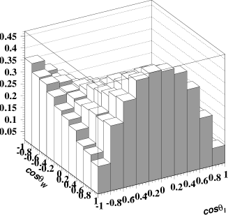
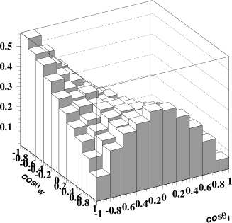
(a)		(b)

Figure 3: Normalized differential decay distributions (a) for $(f_{1},f_{2})=(1,0)$, and (b) for $(f_{1},f_{2})=(1,0.3)$. They are normalized to unity upon integration.

3 Effective spin reconstruction

At hadron colliders, top quarks are produced dominantly through $t\bar{t}$ production processes. At Tevatron, 85% of the produced $t\bar{t}$ pairs come from $q\bar{q}$ initial states, while 15% come from $gg$ initial states. On the other hand, at LHC, the corresponding fractions are 10% ($q\bar{q}$) and 90% ($gg$), respectively. At these colliders, polarization of the produced top quarks is rather small: at tree level, produced top quarks are unpolarized; at NLO, polarization of top quarks is reported to be very small [29]. Therefore, a priori, the spin orientation of a produced top quark is unknown. This is in contrast to $e^{+}e^{-}$ colliders, where sizable polarization of top quarks is expected due to parity-violating nature of the interactions in the top production process.

In our analysis of the anomalous couplings, we want to utilize correlations between the top quark spin direction and the distribution of its decay daughters. As already mentioned, in most of the existing analyses, people have considered correlations between the top spin and antitop spin in the $t\bar{t}$ production process. In principle we may use these correlations to reconstruct the spin direction of the parent top quark. Namely, we may use the information of the decay distributions on the antitop side to reconstruct the top spin direction, and then examine the correlation between the top spin direction and the distribution of its decay products. A serious deficit of such methods is that they are quite complicated. For instance, the direction of the down-type quark in the hadronic decay of antitop quark is maximally correlated with the antitop spin. Hence, in order to reconstruct the spin of the antitop quark, we should distinguish the charges of the quarks from $W$. This is a highly non-trivial task and we anticipate that rather large systematic errors will be involved before eventually reconstructing the top quark spin. On the other hand, if we want to use semi-leptonic decays both on top and antitop sides, we suffer from lack of statistics, as well as it is non-trivial to solve kinematics due to the two missing momenta of the neutrinos.

Here we take another route for reconstructing (effectively) the top quark spin. We use the correlation between the top spin and the direction of the charged lepton in the top decay for reconstructing the parent top quark’s spin, and then use it to analyze the decay anomalous couplings of the same top quark. Since we both reconstruct the spin and analyze the spin-dependent decay distribution using the same top decay process, we should make sure that we use independent correlations in the former and latter procedures to avoid obtaining a meaningless outcome. For this purpose, we take advantage of the following facts: (1) Within the SM, the charged lepton is known to be the best analyzer of the parent top quark’s spin and is produced preferentially in the direction of the top spin [30]. (2) The angular distribution of the charged lepton with respect to the top spin direction (after all other kinematical variables are integrated out) is hardly affected by the anomalous couplings of top quark, if the anomalous couplings are small [31]. Therefore, we may project the direction of the charged lepton onto an appropriate spin basis; then the reconstructed top quark spin is scarcely affected by existence of the anomalous couplings $f_{1}$ and $f_{2}$ when they are small. It follows that this spin direction is useful in testing the differential decay distribution described in the previous section, which is sensitive to the anomalous couplings.

Provided that produced top quarks are perfectly unpolarized, and provided that we disregard kinematical cuts and acceptance corrections, there is no difference on which spin basis we choose to project the direction of the charged lepton. Suppose we choose for the basis-axis an arbitrary unit vector $\vec{n}$ in the top rest frame. Then, if the lepton is emitted on the same side as $\vec{n}$, i.e. if ${\vec{n}\cdot\vec{p}_{l}}>0$ ($\vec{p}_{l}$ is the lepton momentum in the top rest frame), we define the “spin vector” to be $\vec{n}$; on the other hand, if ${\vec{n}\cdot\vec{p}_{l}}<0$, we define the “spin vector” to be $-\vec{n}$. The differential decay distribution $d\Gamma/d\cos\theta_{W}d\cos\theta_{l}$ with respect to thus defined “spin vector” can be computed analytically, which we present in the Appendix.

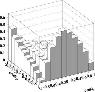
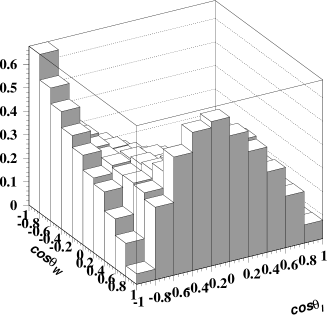
(a)		(b)

Figure 4: Normalized differential decay distributions using the reconstructed effective spin direction ${\rm sign}({\vec{n}\cdot\vec{p}_{l}})\vec{n}$ for (a) $(f_{1},f_{2})=(1,0)$, and (b) $(f_{1},f_{2})=(1,0.3)$. These figures reproduce well the original distributions in Figs. 3.

In Figs. 4, we show this double angular distribution for $(f_{1},f_{2})=(1,0)$ and $(1,0.3)$. One can see that the distributions approximate the corresponding distributions in Figs. 3, which were computed using the spin direction of a polarized top quark. Qualitative features of the bulk distribution shape as well as of the dependence on $f_{2}/f_{1}$ are reproduced. It is this approximation to (reproduction of) the original double angular distribution that guarantees a good efficiency of our spin reconstruction method in the analysis of the anomalous couplings. See [24] for the study on theoretical aspects of the reconstructed spin direction in this method.

In practice, if we take into account realistic experimental conditions, different choice of spin basis (axis) $\vec{n}$ leads to different sensitivities to the anomalous couplings, due to effects of kinematical cuts. Here, we examine three types of spin basis that have been analyzed in the literature, then we choose the basis which is most suited for our analysis.

The beamline basis [15] is to take the spin axis ($\vec{n}$) to be either of the initial beamline direction in the $t\bar{t}$ c.m. frame; the helicity basis is to take $\vec{n}$ to be the direction of top quark in the $t\bar{t}$ c.m. frame; the off-diagonal basis is defined to be a linear combination of the former two bases in such a way to maximize the correlation between the $t$ and $\bar{t}$ spins [17]. Advantages and disadvantages of these bases have been studied in the context of spin correlations between $t$ and $\bar{t}$ in the $t\bar{t}$ production processes [14, 15, 16, 17, 18]. Nevertheless, these are irrelevant in our spin reconstruction method, since we are concerned only with the top quark (or antitop quark) side. What are relevant in our analysis are the effects of cuts and acceptance corrections. If we use the beamline basis, $E_{T}$ (transverse energy) and $|\eta|$ (pseudorapidity) cuts for leptons and jets strongly distort the double angular distribution $d\Gamma/d\cos\theta_{W}d\cos\theta_{l}$. This is because small $E_{T}$ and large $|\eta|$ regions correspond to the regions $\cos\theta_{W}\simeq\pm 1$ in this basis, and events that fall into these kinematical regions are rejected. In particular, a large part of the enhancement of the $f_{2}/f_{1}$ effects in the region $\cos\theta_{W}\sim-1$, $\cos\theta_{l}\sim-1$ is lost. At Tevatron, the status of the off-diagonal basis is somewhat similar to the beamline basis, since the off-diagonal basis is not very different from the beamline basis at Tevatron energies. (At LHC, there is no good definition of the off-diagonal basis.) The helicity basis turns out to be an optimal choice for our purpose, since this basis points to every direction in the detectors. After integrating over all top quark directions, effects of the cuts are averaged over and no significant distortion from the original distribution is found.

Taking these into account, we define an effective spin direction by a projection of the lepton direction onto the helicity basis:

$$\vec{S}_{\rm SH}=\mathrm{sign}(\cos\Theta)\times\frac{\vec{p}_{t}}{|\vec{p}_{t}|}\quad,$$ (8)

where $\Theta$ is the angle between the charged lepton and the top helicity direction $\vec{p}_{t}/|\vec{p}_{t}|$ (opposite of the antitop direction) in the top rest frame. We refer to the above effective spin direction as signed-helicity (SH) direction.

We conclude that the signed-helicity direction (8) is a valid spin direction in studying the double angular distribution $d\Gamma/d\cos\theta_{W}d\cos\theta_{l}$. It is also important that the dependence of the distribution on the anomalous couplings is approximately reproduced in this spin reconstruction method.

4 Monte Carlo simulation

In order to estimate the sensitivity for the anomalous couplings in the top decay, we perform Monte Carlo (MC) event generation and detector simulations. The events are produced with both Tevatron Run II ($p\bar{p}$ collisions in $\sqrt{s}$ = 1.96 TeV) and LHC ($pp$ collisions in $\sqrt{s}$ = 14 TeV) conditions.

The event generation for the $t\bar{t}$ signal samples is implemented by GR@PPA event generator [32] interfaced by PYTHIA v6.226 showering MC [33]. The GR@PPA produces the hard process based on the $t\bar{t}$ matrix element calculation at the tree level. The whole decay chain of the top quark is included in the diagram calculation, so that the spin correlations in the top decay are fully reproduced. The anomalous couplings in the top decay are also included. PYTHIA performs fragmentation, parton showering, and hadronization. On the other hand, underlying events are produced by PYTHIA alone, using the parameters tuned to reproduce the Tevatron real data.

The detector simulation is performed by smearing energies for the stable particles deposited into a proper segmentation of the calorimeter geometry. The detector is assumed to stretch in absolute pseudorapidity ($|\eta|$) up to 3.0 and be segmented by 0.1 $\eta$ bins and 15${}^{\circ}\phi$ (azimuthal) bins. The transverse energies $E_{T}$ for undecayed particles are summed up in each bin and are smeared by Gaussian distribution with 75% $\times$ $\sqrt{E_{T}}$ standard deviation in GeV. As for leptons, we replace their measured momenta by the values at the generator level.

Although our MC simulations are not fully realistic, we consider them to be useful for giving rough estimates of the sensitivity to the anomalous couplings before performing full simulations. In particular, as for Tevatron experiments, our MC simulation would give quite reasonable results. On the other hand, as for LHC studies, there are some other important ingredients that should be taken into account before giving more realistic estimates of the sensitivity. Among them, the most important effects would be those of extra jets events, i.e. $t\bar{t}+n$-jets events, which are not included in our event generation. Their effects are expected to be small at Tevatron.

A jet is clustered by PYCELL routine in PYTHIA with cone size 0.4. We do not simulate $b$ tagging. Instead a $b$-jet is identified as the nearest jet with the minimum separation $\Delta R$ between a jet and a $b$-quark at the generator level. The separation ($\Delta R$) is defined as

$$\Delta R\;=\;\sqrt{\Delta\phi^{2}+\Delta\eta^{2}}\quad,$$ (9)

where $\Delta\phi$ and $\Delta\eta$ are the separation in the azimuthal angle and the pseudorapidity for every pair of a jet and $b$-quark at the generator level, respectively.

We select the $lepton+jets$ channel in the $t\bar{t}$ production process by requiring to pass the cuts

          Tevatron LHC lepton $p_{T}\;\geq\;20\;\mathrm{GeV}$, $|\eta|\;\leq\;1.0$ $p_{T}\;\geq\;20\;\mathrm{GeV}$, $|\eta|\;\leq\;2.5$ $b$–jet $E_{T}\;\geq\;15\;\mathrm{GeV}$, $|\eta|\;\leq\;1.0$ $E_{T}\;\geq\;30\;\mathrm{GeV}$, $|\eta|\;\leq\;2.5$ other jet $E_{T}\;\geq\;15\;\mathrm{GeV}$, $|\eta|\;\leq\;2.0$ $E_{T}\;\geq\;30\;\mathrm{GeV}$, $|\eta|\;\leq\;2.5$ $E/\hskip 0.28453pt_{T}\,\geq\;20\;\mathrm{GeV}$ $E/\hskip 0.28453pt_{T}\,\geq\;20\;\mathrm{GeV}$

where $E/\hskip 0.28453pt_{T}$ is the missing transverse energy calculated by the vector summation of the candidate lepton and four jets. We require two $b$-jets within at least 4 jets in each event.

The detection efficiency is 1.2% including acceptance corrections and branching fraction of $t\bar{t}$ events to the $lepton+jets$ channel, with 25% double $b$-tagging efficiency at Tevatron condition; the corresponding detection efficiency is 2.3 % with 60% double $b$-tagging efficiency at LHC condition. Kinematical acceptance fluctuates only within 0.5% for various values of the anomalous couplings.

5 Event reconstruction

We measure the double angular distribution of $W$ and the charged lepton. For this purpose, it is important to reconstruct the full event topology of top quark events. The reconstruction of the $t\bar{t}$ event topology is performed by a likelihood method on event by event basis, using the $lepton+jets$ events selected as above. Our kinematical likelihood event reconstruction is based on that of [27], which is a dedicated study for top quark reconstruction at future $e^{+}e^{-}$ linear colliders. In order to apply it to hadron collider experiments, some modifications are implemented. We assume that the energy-momentum of leptons and directions of jets can be measured accurately. Thus, for the $lepton+jets$ channel, we treat only 5 parameters out of 16 kinematical parameters as unknown. These 5 parameters are assigned to be the $E_{T}$ of jets and the boost vector of $t\bar{t}$ c.m. system along the beam axis. We neglect the transverse momentum of the $t\bar{t}$ system. The fit is constrained by the top quark mass, $W$ mass and parton distribution function (PDF). Our likelihood function is formed as

$$L\;=\Bigl{[}\prod_{i=1}^{4}P_{jet}^{i}(E_{T}^{exp.},E_{T}^{gen.})\Bigr{]}\cdot P_{\Gamma_{W^{+}}}\cdot P_{\Gamma_{W^{-}}}\cdot P_{\Gamma_{t}}\cdot P_{\Gamma_{\bar{t}}}\cdot P_{Z_{PDF}}^{t\bar{t}}\quad,$$ (10)

where $P_{jet}^{i}$ is the jet response function that relates the measured jet energy to the corresponding parton-level energy; $P_{\Gamma_{W^{+}}}$, $P_{\Gamma_{W^{-}}}$, $P_{\Gamma_{t}}$ and $P_{\Gamma_{\bar{t}}}$ are Breit-Wigner functions for $W^{+}$, $W^{-}$, $t$ and $\bar{t}$, respectively; $P_{Z_{PDF}}^{t\bar{t}}$ constrains the boost momentum of the $t\bar{t}$ c.m. system by PDF function. Whenever more than one solution for jet assignment is found in each $t\bar{t}$ candidate event, we take the one that maximizes the likelihood function.

The jet response functions are constructed for the light-quark jets from $W$ and for the $b$-jets separately in the following manner. A single parton generator is used to estimate them. A parton with a certain fixed energy and direction is generated and passed through the detector simulation. The energy of the reconstructed jet at the detector level is fitted by Gaussian distribution and is defined to be the probability density for the given energy and direction of the parent parton. We iterate this procedure with various energies and directions, and define jet energy scales of the responses in the calorimeter positions as the jet response functions.

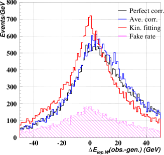
(a)		(b)
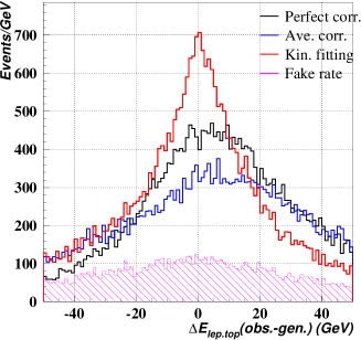
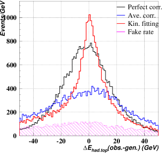
(c)		(d)

Figure 5: Deviations between the parton energies at the generator level and corrected jet energies at the detector level for (a) leptonically decayed $W$ boson, (b) hadronically decayed $W$ boson, (c) leptonically decayed top quark, and (d) hadronically decayed top quark.

Let us demonstrate how well the parton kinematics are reconstructed. In Figs. 5 we show the difference between the parton energy at the generator level and the energy determined by the fit at the detector level: we show the energy differences for (a) the leptonically-decayed $W$ boson, (b) the hadronically-decayed $W$ boson, (c) the leptonically-decayed top quark, and (d) the hadronically-decayed top quark, respectively. The fake contributions are also shown as hatched regions, which correspond to the events that include jets not assigned in correct combinations by the fit. (We define that jets are correctly assigned, if the directions of all jets are matched with those of the original partons within jet cone radius of 0.4.) For comparison, the other reconstruction methods “perfect correction” and “average correction” are also presented in the figures. With the “perfect correction”, the jet energy is defined to be the corresponding parton energy at the generator level smeared with a finite detector resolution. With the “average correction”, the jet energy is uniformly corrected by the jet energy scale for the mean value. Note that the fake contributions are not included for these two correction methods.

From Figs. 5, we can see that the likelihood fitting method reproduces the event kinematics considerably better than the other two methods. Quality of the energy reconstructions of $W$ and top quark is worse on the leptonic side than on the hadronic side. This follows from a poorer resolution for the neutrino momentum on the leptonic side, which is defined as the opposite of the vector summation of all (four) jets and lepton in the $t\bar{t}$ c.m. frame. On the other hand, $W$ and top quark on the hadronic side are reconstructed using the two and three jets, respectively. One sees that, in the tail regions of the distributions in the figures, the correctly assigned events are suppressed, which also shows that the likelihood fitting works as expected.

Using the reconstructed momenta of $t$ and $\bar{t}$, we reconstruct the effective top spin according to the signed-helicity method Eq. (8) as follows. The top helicity axis is defined in the top quark rest frame as (the opposite of) the direction of the momentum of the hadronically-decayed antitop quark, which sequentially decayed into three jets. The sign of the top spin is defined by the direction of the charged lepton in the top rest frame. The reconstructed top quark momentum is also used to measure the helicity angle of the charged lepton, since the original direction of $W$ in the $W$ rest frame is equivalent to the opposite of the leptonically-decayed top quark direction in the $W$ rest frame (see Sec. 2).

6 Sensitivity study

In this section, we study the sensitivity for the anomalous couplings using the $lepton+jets$ events reconstructed by the kinematical likelihood fitting.

We show in Figs. 6 the double angular distributions $d\Gamma/d\cos\theta_{W}\cos\theta_{l}$ using the MC events, after event selection and event reconstruction by the kinematical likelihood fitting. Compare with the corresponding parton distributions at the generator level in Figs. 4. One can see that, even after cuts, the dependence on the anomalous couplings remains in the $W_{T}$ region ($\cos\theta_{W}\sim-1$, $\cos\theta_{l}\sim-1$).

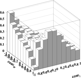
(a)		(b)

Figure 6: Normalized differential decay distributions using the signed-helicity direction after event reconstruction and kinematical cuts (a) for $(f_{1},f_{2})=(1,0)$, and (b) for $(f_{1},f_{2})=(1,0.3)$.

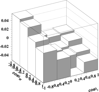
Figure 7: Deviation of the normalized angular distribution when the anomalous couplings are varied from $(f_{1},f_{2})=(1,0)$ to (1, 0.3).

The difference between the angular distributions corresponding to the anomalous couplings ($f_{1}$,$f_{2}$) = (1,0.3) and (1,0) is shown in Fig. 7. The difference is maximized in the $W_{T}$ region ($\cos\theta_{W}\sim-1$, $\cos\theta_{l}\sim-1$) and minimized in its diagonal opposite region ($\cos\theta_{W}\sim 1$, $\cos\theta_{l}\sim 1$). The other two (diagonal) regions have weaker dependences on the anomalous couplings. When signal statistics is small or the background contribution is not well-understood, a simple but not elaborate method to determine the anomalous couplings would be practical for a first analysis. Hence, we divide the kinematical region into 4 regions and simply count the number of events in each region. The regions are defined as follows:

$$\begin{array}[]{lrccrcl}\mathrm{Region\ A}:&-1&\leq\;\cos\theta_{W}\;\leq\;0&\quad\mathrm{and}&-1&\leq\;\cos\theta_{l}\;\leq\;0&\\ \mathrm{Region\ B}:&-1&\leq\;\cos\theta_{W}\;\leq\;0&\quad\mathrm{and}&0&\leq\;\cos\theta_{l}\;\leq\;1&\\ \mathrm{Region\ C}:&0&\leq\;\cos\theta_{W}\;\leq\;1&\quad\mathrm{and}&-1&\leq\;\cos\theta_{l}\;\leq\;0&\\ \mathrm{Region\ D}:&0&\leq\;\cos\theta_{W}\;\leq\;1&\quad\mathrm{and}&0&\leq\;\cos\theta_{l}\;\leq\;1&\quad.\\ \end{array}$$ (11)

The dependences of the event fractions in these regions on the anomalous couplings are shown in Fig. 8. The regions A and D are the regions most sensitive to the anomalous couplings, while the regions B and C are less sensitive regions. We can see that the event fraction in region A increases with $f_{2}$/$f_{1}$ when $f_{2}$/$f_{1}$ $>$ 0, and takes a minimum value around $f_{2}$/$f_{1}\approx-0.45$, and then increases again if we lower $f_{2}$/$f_{1}$ below $-0.45$. The event fraction in region D has an opposite behavior to that of region A. All the event fractions take maximum or minimum values around $f_{2}$/$f_{1}=-M_{W}/M_{t}\approx-0.45$, where the transverse component of $W$ is canceled; cf. Eq. (7).

We fit the MC data (shown by discrete points in Fig. 8) by analytic functions as follows. In an ideal case, we can integrate Eq. (22) analytically over each of the regions A–D. The event fraction distributed in each region takes a form

$$F^{i}(x)\;=\;\frac{a^{i}_{1}x^{2}\;+\;a^{i}_{2}x\;+\;a^{i}_{3}}{\widetilde{\Gamma}_{\rm tot}(x)}\quad,~{}~{}~{}~{}~{}x=\frac{f_{2}}{f_{1}},~{}~{}~{}~{}~{}i={\rm A,B,C,D}$$ (12)

where ${\widetilde{\Gamma}_{\rm tot}(x)}=\Gamma_{t\to bW}(f_{1},f_{2})/|f_{1}|^{2}$. ($\Gamma_{t\to bW}(f_{1},f_{2})$ is the partial decay width of the top quark.) Parameters $a^{i}_{1},a^{i}_{2},a^{i}_{3}$ can be expressed analytically in terms of the top and $W$ masses. Note that since $f_{1}$ only contributes to the normalization of the differential angular distribution which does not affect the shape of the distribution, the event fractions depend only on $x=f_{2}/f_{1}$ regardless of various choices of $f_{1}$ and $f_{2}$.

In a realistic case, the distributions are affected by the finite resolution of detectors, by cuts, by fake contributions, etc. Here, we fit the event fractions generated by MC simulation with high statistics by the same functional form as in Eq. (11), taking $a^{i}_{1},a^{i}_{2},a^{i}_{3}$ as the parameters to be determined by the fit. The sum of the event fractions in four regions is normalized to one, so that 9 parameters are decided by minimizing the fitting $\chi^{2}$. The MC data and fitting results of the event fractions in each region are shown as functions of $f_{2}$/$f_{1}$ in Fig. 8. The $\chi^{2}$ minimum per each degree of freedom takes a reasonable value $\approx 1.20$. The functions $F^{i}(x)$ determined by the fit are used to estimate sensitivity to the anomalous couplings.

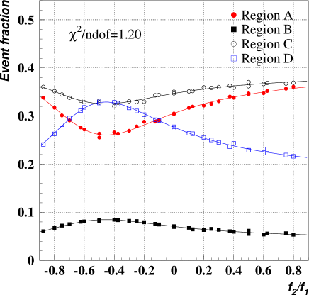
Figure 8: MC data and fitting results of the event fractions in each region as functions of $f_{2}$/$f_{1}$. Each region is defined in Eq. (11).

In Table 1, the expected bounds on the coupling ratio at 95% C.L. are shown, corresponding to 100 and 1000 selected events (after cuts) for the Tevatron experiment and 100k selected events (after cuts) for the LHC experiment, respectively. Input parameters of the MC simulations are taken as $(f_{1},f_{2})=(1,0)$ (tree-level SM values). Only statistical errors are taken into account to obtain the allowed regions. For comparison, we present the allowed regions using an ideal off-diagonal direction (for Tevatron), in which the spin direction is reconstructed using the off-diagonal basis with the sign ambiguity resolved by looking into the information at the generator level; we may consider that this ideal off-diagonal direction approximates the true spin direction well, so that the corresponding results can be used as references (although these include effects of kinematical cuts as well as contamination by fake events). We also present the allowed regions using only the events with correct assignment of two $b$-jets using the signed helicity direction.

In Table 1, the bounds using the signed helicity direction are not very different from those using the ideal off-diagonal spin direction at Tevatron. Since the latter results can be regarded as references for optimal reconstruction of the top spin, it is seen that the signed helicity direction is quite efficient for this analysis. In addition, the sensitivities can be improved if we can remove misassignment of the $b$-jets.

Although it is obvious that the expected bound becomes tighter as the number of events increases, the way the bound shrinks with statistics is rather peculiar. This is because the event fractions have characteristic (non-linear) $f_{2}/f_{1}$-dependences, almost symmetric under reflection with respect to $f_{2}/f_{1}\approx-0.45$; see Fig. 8. At low statistics (100 events or less), the bound on $f_{2}/f_{1}$ is fairly loose. When the statistics is increased, the bound does not simply scale with $1/\sqrt{N}$ but becomes narrower much faster, with a two-fold ambiguity that remains, i.e., the regions around $f_{2}/f_{1}\approx 0$ and $f_{2}/f_{1}\approx-0.75$ cannot be discriminated. Once the number of events exceeds a few hundred, the bound scales with $1/\sqrt{N}$, since the dependences of the event fractions can be approximated by linear responses. This gives a motivation to increase the number of events (after cuts) at least beyond a few hundred at Tevatron experiment.

Finally, we show the expected excluded regions in the $(f_{2},f_{1})$-plane at 95% C.L. for the Tevatron case in Fig. 9. We anticipate that our method allows us to cover a wide region in the parameter space even in this simplified counting experiment.

	Tevatron ($\sqrt{s}=1.96$ TeV)		LHC ($\sqrt{s}=14$ TeV)
Number of events	100	1000	100k
Signed-helicity direction	$-0.93$ $<$ $\frac{f_{2}}{f_{1}}$ $<$ 0.57	$-0.12$ $<$ $\frac{f_{2}}{f_{1}}$ $<$ 0.14,	$-0.01$ $<$ $\frac{f_{2}}{f_{1}}$ $<$ 0.01,
		$-0.81$ $<\frac{f_{2}}{f_{1}}<$ $-0.70$	$-0.74$ $<\frac{f_{2}}{f_{1}}<$ $-0.72$
Ideal off-diagonal direction	$-0.84$ $<$ $\frac{f_{2}}{f_{1}}$ $<$ 0.50	$-0.11$ $<$ $\frac{f_{2}}{f_{1}}$ $<$ 0.12,	Not applicable
		$-0.73$ $<\frac{f_{2}}{f_{1}}<$ $-0.61$
Signed-helicity direction	$-0.29$ $<$ $\frac{f_{2}}{f_{1}}$ $<$ 0.39,	$-0.09$ $<$ $\frac{f_{2}}{f_{1}}$ $<$ 0.10,	$-0.01$ $<$ $\frac{f_{2}}{f_{1}}$ $<$ 0.01,
with correct $b$ assignment	$-0.89$ $<\frac{f_{2}}{f_{1}}<$ $-0.59$	$-0.80$ $<\frac{f_{2}}{f_{1}}<$ $-0.71$	$-0.75$ $<\frac{f_{2}}{f_{1}}<$ $-0.74$

Table 1: Expected bounds at 95% C.L. corresponding to 100 and 1000 events (after cuts) for Tevatron and 100k events (after cuts) for LHC. Input parameters of the MC simulations are taken as $(f_{1},f_{2})=(1,0)$. Only statistical errors are taken into account. For comparison, the bounds using an ideal off-diagonal direction, and those using only the events with correct assignment of two $b$-jets in the signed helicity method are presented.

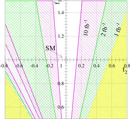
Figure 9: Expected excluded regions at 95% C.L. in the $(f_{2},f_{1})$-plane at Tevatron. The shaded regions correspond to 1 fb^-1, 2 fb^-1, and 10 fb^-1 integrated luminosities, respectively. The input SM point is located at ($f_{2}$,$f_{1}$)=(0,1).

7 Conclusions

We have studied sensitivities to the top quark decay anomalous couplings $f_{1}$ and $f_{2}$ at hadron colliders, taking into account realistic experimental conditions expected at Tevatron and LHC. Since large samples of top quarks are expected at these colliders, and since the decay processes of the top quark can be predicted reliably by perturbative QCD, we can achieve high sensitivities to the anomalous couplings from detailed studies of the top quark decay processes. We used a likelihood method to fully reconstruct the momenta of the partons in the lepton+4 jets mode. Furthermore, we devised a new method for reconstructing an effective spin direction Eq. (8) (referred as signed-helicity direction) of the leptonically-decayed top quark. It is defined as the projection of the lepton direction onto the top helicity axis in the top rest frame. This method does not require reconstruction of the spin of the hadronically-decayed top quark, hence it helps to elude possibly large systematic uncertainties. These two techniques, when used in combination, revealed to be quite powerful for the sensitivity study.

We analyzed a double angular distribution $d\Gamma(t\to bl\nu)/d\cos\theta_{W}d\cos\theta_{l}$. The $W_{T}$ region $\cos\theta_{W}\sim-1$, $\cos\theta_{l}\sim-1$ of the distribution is sensitive to the ratio of the anomalous couplings $f_{2}/f_{1}$. We confirmed that this feature is preserved even after kinematical cuts. We note that if we choose a spin axis other than top helicity basis, such as beamline basis or off-diagonal basis, sensitivity to $f_{2}/f_{1}$ is substantially reduced due to effects by the kinematical cuts.

In order to give reliable estimates, we developed an event generator incorporating in the matrix element proper spin correlations of partons as well as the anomalous couplings in the top decay vertices. We also simulate the detector effects by assuming a simple geometry and energy resolutions based on the CDF and ATLAS detectors for Tevatron and LHC experiments, respectively. After event selection, the event kinematics are reconstructed by the kinematical likelihood fitting on an event by event basis. It not only improves the jet energy scale from the measured jet energy to the corresponding parton energy but also helps to select the correct configuration of the jets in the top event topology. Furthermore, the likelihood fitting method improves reconstruction of the hadronically-decayed top quark’s energy and momentum, which is directly reflected to the determination of the top spin direction as well as lepton helicity angle.

As a first analysis, we simply counted the event fractions of the double angular distribution divided into 4 regions. Then we performed $\chi^{2}$–fits to these event fractions in order to find sensitivities to $f_{2}/f_{1}$. The results can be summarized as follows. The bounds obtained at 95% C.L. read

$$\begin{array}[]{cl}-0.93<\frac{f_{2}}{f_{1}}<0.57&\mbox{for 100 reconstructed events at Tevatron,}\\ -0.81<\frac{f_{2}}{f_{1}}<-0.70,~{}~{}-0.12<\frac{f_{2}}{f_{1}}<0.14&\mbox{for 1000 reconstructed events at Tevatron,}\\ -0.74<\frac{f_{2}}{f_{1}}<-0.72,~{}~{}-0.01<\frac{f_{2}}{f_{1}}<0.01&\mbox{for 100k reconstructed events at LHC}.\end{array}$$ (16)

We took into account only the statistical errors and neglected systematic errors. Due to characteristic dependences of the event fractions on $f_{2}/f_{1}$, the bound on $f_{2}/f_{1}$ shrinks quickly as the number of top quark events increases up to a few hundred. For more events, the bound scales with $1/\sqrt{N}$, and there remains a two-fold ambiguity for the allowed ranges of $f_{2}/f_{1}$.

Although some simplifications have been made, we consider that our MC study for the Tevatron experiment imitates realistic experimental conditions closely enough to give reasonable estimates for the sensitivities to the anomalous couplings. On the other hand, as for the LHC case, some important ingredients are still missing in the MC simulation (the most important one would be $t\bar{t}+n$-jets events), so our results should be taken as first rough estimates.

Since our methods for event reconstruction and effective top spin reconstruction are fairly simple, we would expect that they can be applied to other analyses, such as precise determination of $W$ polarization states in top decay.

Appendix: Decay angular distribution using the signed-helicity spin direction

In this Appendix, we present the analytic formula for the double angular distribution in the decay of top quark, $d\Gamma/d\cos\theta_{W}d\cos\theta_{l}$, when we use the lepton direction projected onto any spin basis for the reconstructed top quark spin direction. (When we choose the helicity basis, we call the reconstructed spin direction as “signed-helicity” direction.) We assume the parent top quark to be unpolarized and neglect the effects of kinematical cuts.

An arbitrary unit vector $\vec{n}$ is chosen as the spin axis in the top rest frame. Then, if ${\vec{n}\cdot\vec{p}_{l}}>0$, we define the “spin vector” to be $\vec{n}$ whereas, if ${\vec{n}\cdot\vec{p}_{l}}<0$, we define the “spin vector” to be $-\vec{n}$. The differential decay distribution $d\Gamma/d\cos\theta_{W}d\cos\theta_{l}$ with respect to thus defined “spin vector” can be computed analytically as follows. The angle $\Theta$ between $\vec{n}$ and $\vec{p}_{l}$ is given by

$$\cos\Theta\equiv\frac{\vec{n}\cdot\vec{p}_{l}}{|\vec{p}_{l}|}=\frac{\sqrt{1-\beta_{W}^{2}}}{1+\beta_{W}\cos\theta_{l}}\left(\sin\theta_{l}\cos\phi_{l}\sin\theta_{W}+\frac{\cos\theta_{l}+\beta_{W}}{\sqrt{1-\beta_{W}^{2}}}\cos\theta_{W}\right),$$ (17)

$$\beta_{W}=\frac{M_{t}^{2}-M_{W}^{2}}{M_{t}^{2}+M_{W}^{2}},$$ (18)

where $\theta_{W}$ and $\phi_{l}$ are defined as in Fig. 2 with respect to $\vec{n}$. Since the definition of the spin vector is reversed when $\cos\Theta<0$, in this case we need to redefine the angles to be $\theta_{W}\to\pi-\theta_{W}$ and $\phi_{l}\to\phi_{l}+\pi$ in the cross section formula. Therefore, noting that the initial top quark is unpolarized, the double angular distribution is given by

$$\left[\frac{d\Gamma(t\rightarrow bW\!\rightarrow bl\nu)}{d\cos\theta_{W}d\cos\theta_{l}}\right]_{\rm SH}$$

$$=\int_{\cos\Theta>0}\!\!\!\!\!\!d\phi_{l}\,\left[\frac{d\Gamma(t\rightarrow bW\!\rightarrow bl\nu)}{d\cos\theta_{W}d\cos\theta_{l}d\phi_{l}}\right]_{\rm unpol.}+\left[\int_{\cos\Theta<0}\!\!\!\!\!\!d\phi_{l}\,\left[\frac{d\Gamma(t\rightarrow bW\!\rightarrow bl\nu)}{d\cos\theta_{W}d\cos\theta_{l}d\phi_{l}}\right]_{\rm unpol.}\right]_{\begin{array}[]{l}\scriptstyle\theta_{W}\to\pi-\theta_{W}\\ \scriptstyle\phi_{l}\to\phi_{l}+\pi\end{array}}$$ (21)

$$=\left[\frac{d\Gamma(t\rightarrow bW\!\rightarrow bl\nu)}{d\cos\theta_{W}d\cos\theta_{l}d\phi_{l}}\right]_{\rm unpol.}\times 2\,g(y),$$ (22)

where

$$y=-\frac{\cos\theta_{l}+\beta_{W}}{\sqrt{1-\beta_{W}^{2}}}\,\frac{\cot\theta_{W}}{\sin\theta_{l}},$$ (23)

$$g(x)=\left\{\begin{array}[]{ll}0&\mbox{if $x\geq 1$}\\ 2\pi&\mbox{if $x\leq-1$}\\ \pi-2\arcsin x&\mbox{if $-1<x<1$}\end{array}\right..$$ (27)

The decay distribution from an unpolarized top quark is given by

$$\left[\frac{d\Gamma(t\rightarrow bW\!\rightarrow bl\nu)}{d\cos\theta_{W}d\cos\theta_{l}d\phi_{l}}\right]_{\rm unpol.}=\frac{1}{4}\,A\,\biggl{[}\Bigl{(}f_{1}\frac{M_{t}}{M_{W}}+f_{2}\Bigr{)}^{2}\,\sin^{2}\theta_{l}+4\,\Bigl{(}f_{1}+f_{2}\frac{M_{t}}{M_{W}}\Bigr{)}^{2}\,\sin^{4}\frac{\theta_{l}}{2}\biggr{]}\,.$$ (28)

It is independent of $\theta_{W}$ and $\phi_{l}$, since there is no reference spin vector.

References

- [1]
- [2] CDF Collaboration, D0 Collaboration and Tevatron Electroweak Working Group, hep-ex/0507091.
-
[3]
D. Acosta et al. (CDF Collaboration),
Phys. Rev. Lett. 95 (2005) 102002;
D0 Collaboration,
http://www-do.fnal.gov/Run2Physics/WWW/results/prelim/TOP/T14/T14.pdf. -
[4]
A. Abulencia, et al. (CDF Collaboration),
hep-ex/0511023;
V. Abazov, et al. (D0 Collaboration), Phys. Rev. D 72 (2005) 011104. - [5] M. Hosch, K. Whisnant, and B. Young, Phys. Rev. D 55 (1997) 3137.
- [6] K. Hikasa, K. Whisnant, J. Yang, and B. Young, Phys. Rev. D 58 (1998) 114003.
- [7] K. Fujikawa and A. Yamada, Phys. Rev. D 49 (1994) 5890. F. Larios, M.A. Perez and C.P. Yuan, Phys. Lett. B 457 (1999) 334. G. Burdman, M.C. Gonzalez-Garcia and S.F. Novaes, Phys. Rev. D 61 (2000) 114016.
- [8] J. Yang and C. Li, Phys. Lett. B 320 (1994) 117; C. Li, J. Yang, and B. Hu, Phys. Rev. D 48 (5425) 1993; D. Garcia, R. Jiménez, J. Solá and W. Hollik, Nucl. Phys. B 427 (1994) 53; A. Dabelstein, W. Hollik, C. Jünger, R. Jiménez and J. Solá, Nucl. Phys. B 454 (1995) 75; A. Brandenburg and M. Maniatis, Phys. Lett. B 545 (2005) 139.
- [9] J. Cao, R. Oakes, F. Wang, and J. Yang, Phys. Rev. D 68 (2003) 054019.
- [10] Y. Nie, C. Li, Q. Li, J. Liu, and J. Zhao, Phys. Rev. D 71 (2005) 074018.
- [11] X. Wang, Q. Zhang, and Q. Qiao, Phys. Rev. D 71 (2005) 014035.
- [12] C. Chen, F. Larios, and C.-P. Yuan, Phys. Lett. B 631 (2005) 126.
- [13] N. Mahajan, Phys. Rev. D 68 (2003) 095001.
- [14] V. Barger, J. Ohnemus, and R. J. Phillips, Int. J. Phys. A4 (1989) 617; Y. Hara, Prog. Theor. Phys. 86 (1991) 779; T. Arens and L. M. Sehgal, Phys. Lett. B 302 (1993) 501; A. Brandenburg, Phys. Lett. B 388 (1996) 626.
- [15] G. Mahlon and S.J. Parke, Phys. Rev. D 53 (1996) 4886; Phys. Lett. B 411 (1997) 173.
- [16] T. Stelzer and S. Willenbrock, Phys. Lett. B 374 (1996) 169.
- [17] S.J. Park and Y. Shadmi, Phys. Lett. B 387 (1996) 199.
- [18] W. Bernreuther, M. Flesch and P. Haberl, Phys. Rev. D 58 (1998) 114031.
- [19] B. Lampe, Phys. Lett. B 415 (1997) 63.
- [20] G. Altarelli and M. L. Mangano (ed.), Proceedings of the Workshop on Standard model physics (and more) at the LHC, CERN-2000-04, May 2000.
- [21] E. Boos, L. Dudko, and T. Ohl, Eur. Phys. J. C 11 (1999) 473.
- [22] D. Acosta [CDF Collaboration], Phys. Rev. D 71 (2005) 012005.
- [23] V.M. Abazov [D0 Collaboration], hep-ex/0505063.
- [24] Y. Sumino and S. Tsuno, hep-ph/0512205.
-
[25]
G.L. Kane, G.A. Ladinsky and C.P. Yuan, Phys. Rev. D 45 (1992) 124;
K. Whisnant , Phys. Rev. D 56 (1997) 467. -
[26]
N. Cabbibo, Phys. Rev. Lett. 10 (1961) 531;
M. Kobayashi and T. Maskawa, Prog. Theor. Phys. 49 (1973) 652. - [27] K. Ikematsu, K. Fujii, Z. Hioki, Y. Sumino and T. Takahashi, Eur. Phys. J. C 29 (2003) 1.
- [28] M. Fischer, S. Groote, J.G. Korner, M.C. Mauser, and B. Lampe, Phys. Lett. B 451 (1999) 406; M. Fischer, S. Groote, J.G. Korner, and M.C. Mauser, Phys. Rev. D 65 (2002) 054036.
-
[29]
W. Bernreuther , Phys. Lett. B 509 (2001) 53;
W. Bernreuther , Phys. Lett. B 483 (2000) 99. - [30] M. Jeżabek and J.H. Kühn, Phys. Rev. D 48 (1993) R1910; erratum Phys. Rev. D 49 (1994) 4970.
- [31] B. Grza̧dkowski and Z. Hioki, Phys. Lett. B 476 (2000) 87.
- [32] S. Tsuno , Comput. Phys. Commun. 151 (2003) 216.
- [33] T. Sjöstrand, et al., Comput. Phys. Commun. 135 (2001) 238.