A partial wave analysis of the $\pi^{-}\pi^{-}\pi^{+}$ and $\pi^{-}\pi^{0}\pi^{0}$ systems
and the search for a $J^{PC}=1^{-+}$ meson

Abstract

A partial wave analysis (PWA) of the $\pi^{-}\pi^{-}\pi^{+}$ and $\pi^{-}\pi^{0}\pi^{0}$ systems produced in the reaction $\pi^{-}p\to(3\pi)^{-}p$ at 18 GeV/$c$ was carried out using an isobar model assumption. This analysis is based on 3.0M $\pi^{-}\pi^{0}\pi^{0}$ events and 2.6M $\pi^{-}\pi^{-}\pi^{+}$ events and shows production of the $a_{1}(1260)$, $a_{2}(1320)$, $\pi_{2}(1670)$ and $a_{4}(2040)$ resonances. Results of detailed studies of the stability of partial wave fits are presented. An earlier analysis of 250K $\pi^{-}\pi^{-}\pi^{+}$ events from the same experiment showed possible evidence for a $J^{PC}=1^{-+}$ exotic meson with a mass of $\sim$1.6 GeV/$c^{2}$ decaying into $\rho\pi$. In this analysis of a higher statistics sample of the $(3\pi)^{-}$ system in two charged modes we find no evidence of an exotic meson.

I Introduction

In this paper we present a partial wave analysis (PWA) of a high-statistics sample of events corresponding to the production of the $(3\pi)^{-}$ system produced in $\pi^{-}p$ collisions in two modes: $\pi^{-}\pi^{0}\pi^{0}$ and $\pi^{-}\pi^{-}\pi^{+}$. This sample size exceeds, by at least an order of magnitude, the largest published sample size of $3\pi$ events to date. Previous $3\pi$ analyses led to the discovery and/or determination of properties of the $a_{1}(1260)$, $a_{2}(1320)$, $\pi_{2}(1670)$, $\pi(1800)$ and the $a_{4}(2040)$ resonances Ballam68 ; Ascoli70 ; Antipov73 ; Baltay77 ; Daum80a ; Daum80b ; Daum80c ; Daum81 .

In 1998, the E852 collaboration reported evidence for the $\pi_{1}(1600)$, a $J^{PC}=1^{-+}$ exotic hybrid meson with a mass of 1.6 GeV/$c^{2}$ decaying into $\rho\pi$ Adams98 ; Chung02 . That analysis was based on 250,000 events of the reaction $\pi^{-}p\to\pi^{-}\pi^{-}\pi^{+}p$ collected in 1994. We report on the analysis of additional data collected in 1995 including 3.0M events of the reaction $\pi^{-}p\to\pi^{-}\pi^{0}\pi^{0}p$ and 2.6M events of the reaction $\pi^{-}p\to\pi^{-}\pi^{-}\pi^{+}p$.

The identification of exotic mesons requires a PWA to extract signals. The $3\pi$ system provides a particularly attractive venue for such searches since earlier work suggests a rich spectrum of meson resonances. If an exotic meson is produced with relatively small amplitude, its interference with nearby well-established resonances is a sensitive search tool.

In almost all of the published amplitude analyses of the $3\pi$ system, the isobar model was employed – a $3\pi$ system with a particular $J^{PC}$ is produced and decays into a di-pion resonance with well-defined quantum numbers and a bachelor $\pi$ followed by the decay of the di-pion resonance. This assumption is successful in describing many features of the $3\pi$ system and is motivated by the observation that the di-pion effective mass spectrum shows prominent resonance production, for example, the $\rho(770)$ and the $f_{2}(1275)$. The di-pion resonances considered in this analysis include the $f_{0}(980)$, $\rho(770)$, $f_{2}(1275)$ and the $\rho_{3}(1690)$. We also include parametrizations of $S$-wave $\pi\pi$ scattering.

In this analysis, we observe the $a_{1}(1260)$, $a_{2}(1320)$, $\pi_{2}(1670)$ and the $a_{4}(2040)$ in appropriate partial wave intensities and in their relative phase differences. We also searched for, but find no evidence for, the $J^{PC}=1^{-+}$ exotic $\pi_{1}(1600)$ in either the $\pi^{-}\pi^{0}\pi^{0}$ or $\pi^{-}\pi^{-}\pi^{+}$ mode.

In order to extract reliable information from a partial wave analysis it is important to establish a procedure for determining a sufficient set of partial waves. Failure to include important partial waves in the series expansion may lead to inconsistent results and erroneous conclusions. In this paper we describe our procedure for determining a sufficient wave set. That procedure includes a comparison of moments as calculated from PWA solutions with those computed directly from data. We emphasize that this analysis is similar to that of references  Adams98 ; Chung02 in that the same isobar model assumptions are made but the final set of partial waves used is different. Both analyses make the same assumptions about coherence between different partial waves. It is possible that relaxing these coherence assumptions could lead to different results in both analyses.

I.1 General features of the $\bm{(3\pi)^{-}}$ system

The $3\pi$ system with non-zero charge has isospin $I>0$, and, since no flavor exotic mesons have been found, we assume $I=1$. Since a state with an odd number of pions has negative $G$ parity, the relationship $G=C(-1)^{I}$ implies positive $C$ parity for the $(3\pi)^{-}$ system.

The simultaneous observation of the two $(3\pi)^{-}$ modes, $\pi^{-}\pi^{0}\pi^{0}$ and $\pi^{-}\pi^{-}\pi^{+}$, in the same experiment provides important cross checks. Consider the production of resonance $X$ and its subsequent decay into $(3\pi)^{-}$ via an intermediate di-pion resonance. If the intermediate di-pion resonance is an isoscalar, then the yield into $\pi^{-}\pi^{-}\pi^{+}$ should be twice that into $\pi^{-}\pi^{0}\pi^{0}$. Similarly, if the di-pion is an isovector, then there should be equal yields into $\pi^{-}\pi^{-}\pi^{+}$ and $\pi^{-}\pi^{0}\pi^{0}$. Since the $\pi^{-}\pi^{-}\pi^{+}$ and $\pi^{-}\pi^{0}\pi^{0}$ modes rely on different elements of the detector, any misunderstandings in the acceptance would affect the two modes differently and ultimately lead to inconsistent interpretations of the PWA results. This underscores the importance of having these two different modes to validate the analysis.

I.2 Exotic mesons within QCD

Quantum chromodynamics (QCD) predicts a spectrum of mesons beyond the $q\bar{q}$ bound states of the conventional quark model. The spin ($J$), parity ($P$) and charge conjugation ($C$) quantum numbers of a $q\bar{q}$ system are: $\vec{J}=\vec{L}+\vec{S}$ where $\vec{L}$ is the angular momentum between the quarks and $\vec{S}$ is the total quark spin, $P=(-1)^{L+1}$ and $C=(-1)^{L+S}$. The $J^{PC}$ combinations: $0^{+-},1^{-+},2^{+-},\dots$ are not allowed and are called exotic . Lattice QCD Bali2004 and QCD-inspired models predict that the excitation of the gluonic field within a meson leads to hybrid mesons, where the gluonic degrees of freedom allow hybrid mesons to have exotic quantum numbers. The observation of hybrid mesons and measurement of their properties provides experimental input necessary for an understanding of quark and gluon confinement in QCD.

I.3 Organization of this paper

This paper is organized as follows. Section II is a discussion of experimental details, including a description of the apparatus (II.1), event reconstruction and selections (II.2) and distributions in effective mass before and after acceptance corrections (II.3). An overview of the PWA methodology, including selection of the wave set, is given in Section III. Section IV is a presentation of the PWA results for individual partial waves using the wave set used in this analysis and the wave set used in the analysis of references Adams98 ; Chung02 for both the $\pi^{-}\pi^{0}\pi^{0}$ and $\pi^{-}\pi^{-}\pi^{+}$ modes. Section V focuses on the exotic $J^{PC}=1^{-+}$ waves and how the failure to include important $J^{PC}=2^{-+}$ waves could lead to misleading conclusions regarding the existence of an exotic resonance. Section VI discusses studies of systematic uncertainties and the conclusions are presented in Section VII.

II Experimental details

II.1 The experimental apparatus

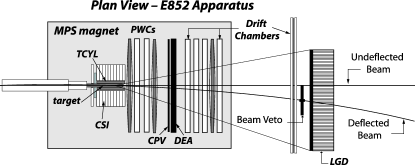
Figure 1: E852 apparatus and the MPS at BNL.

The E852 experiment used the upgraded multiparticle spectrometer (MPS) at the Alternating Gradient Synchrotron (AGS) at Brookhaven National Lab (BNL). The apparatus is described in detail elsewhere Teige99 and is shown schematically in Figure 1. The MPS was upgraded for E852 with the inclusion of a cylindrical drift chamber (TCYL) Bar-yam97 and a cylindrical cesium iodide (CSI) detector AdamsT96 , both concentric with a LH₂ target. Downstream of the target were proportional wire chambers (PWCs) for triggering and tracking, a lead/scintillator array (DEA) and a 3000-element lead glass electromagnetic calorimeter (LGD). The CSI calorimeter consisted of 180 segments – 10 longitudinal segments and 18 azimuthal segments. The DEA had the geometry of a picture frame with a rectangular central hole. A scintillation counter (CPV) was placed just upstream of and matched the geometry of the DEA. The lead glass blocks of the LGD Brabson93 ; Crittenden97 ; Gunter97 ; Lindenbusch97 were each 45 cm long with a transverse area of $4\times 4$ cm² and were arranged in a $284\times 172$ cm² stack with a 2 block $\times$ 2 block beam hole to allow for passage of non-interacting beam particles. The DEA and CSI detected low-energy photons that miss the LGD. The LGD was used to measure energies and positions of photons from $\pi^{0}$ and $\eta$ mesons. The MPS included an analyzing magnet with a 1 T field and drift chambers for tracking. The LH₂ target was 30 cm long and 6 cm in diameter. The beam was an 18.3 GeV/$c$ negatively charged beam consisting mainly (95%) of $\pi^{-}$ and had a momentum bite $\Delta p/p$ of 3% and a momentum resolution $\delta p/p$ of 1%. The target to LGD distance was approximately 5 m. The interacting beam trigger required no signal from a small scintillation counter placed in the path of the beam in coincidence with beam defining counters upstream of the MPS. Event triggers included all-neutral, all charged and a mix of neutral plus charged particle topologies. The neutral particle requirement depended on energy and/or multi-photon effective mass information from the LGD.

II.2 Event reconstruction and selection

We refer to the $\pi^{-}\pi^{0}\pi^{0}p$ system as the neutral mode and the $\pi^{-}\pi^{-}\pi^{+}p$ system as the charged mode. In Tables 1 and 2 the selection requirements and resulting event sample sizes are summarized for the neutral and charged modes respectively. In what follows we discuss details of these requirements 3piE852 .

Table 1: Summary of requirements applied to the data set leading to $\pi^{-}p\to\pi^{-}\pi^{0}\pi^{0}p$.

Cut requirement	Number of Events
Satisfy topology trigger	123,748,800
Require four photons	13,737,265
Confidence level $>0.20$	9,813,524
Beam hole	9,406,003
Vertex location	8,325,895
Recoil proton angle and momentum	6,620,596
CSI and DEA maximum energies	4,939,661
Photon separation	9,579,426
Final sample (all requirements)	3,025,981

Table 2: Summary of requirements applied to the data set leading to $\pi^{-}p\to\pi^{-}\pi^{-}\pi^{+}p$.

Cut requirement	Number of Events
Satisfy topology trigger	78,659,511
No photons	16,796,457
Confidence level $>0.20$	10,157,455
Beam hole	8,038,452
Vertex location	8,038,452
Recoil proton angle and momentum	7,030,216
CSI and DEA maximum energies	4,822,330
$\Delta^{++}$ elimination	9,749,031
Final sample (all requirements)	2,585,776

II.2.1 Initial cuts

The initial requirement was satisfaction of the topology trigger. For both modes a recoil charged track was required through the tracking chamber (TCYL) surrounding the target. The neutral mode required a single forward-going charged particle in the PWCs along with energy deposition in the LGD corresponding to multi-photon effective mass greater than 200 MeV/$c^{2}$. For the charged mode, three forward-going charged particles were required in the PWCs.

Four photons reconstructed in the LGD was the next requirement for the neutral mode. The scatterplot of one di-photon mass against the other di-photon mass is plotted in Figure 2 – there are three such pairings per event in this plot. A clear peak corresponding to $\pi^{0}\pi^{0}$ production is observed. The inset of Figure 2 shows a fit of the $2\gamma$ mass spectrum to a Gaussian and a polynomial. The $\pi^{0}$ mass resolution is 10.4 MeV/$c^{2}$. For the charged mode further cuts required no photons in the event.

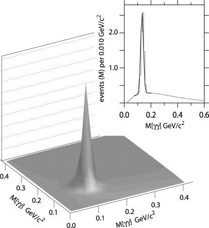
Figure 2: Scatterplot of one di-photon mass against the other di-photon mas (three such pairings per event) for events satisfying the $\pi^{-}\pi^{0}\pi^{0}p$ final state trigger and with four reconstructed photons in the LGD. The inset shows the di-photon mass spectrum with a fit to a Gaussian plus a polynomial. The $\pi^{0}$ mass resolution is 10.4 MeV/$c^{2}$.

The distributions in missing mass squared recoiling against the $3\pi$ system for the neutral and charged modes are shown in Figure 3 (unshaded). Although a charged track corresponding to the recoil proton is required, its momentum is not measured. A kinematic fitting program, SQUAW SQUAW , is used to vary the measured momenta of the the three pions and incoming beam, within errors, to constrain the missing mass to be $m_{p}^{2}$. For the neutral mode, the two di-photon effective masses were constrained to the $\pi^{0}$ mass.

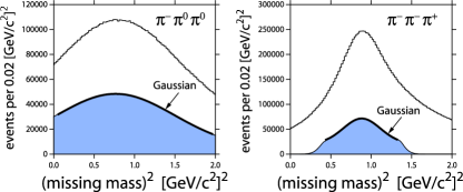
Figure 3: Distribution in missing mass squared recoiling against the $3\pi$ system for the (left) $\pi^{-}\pi^{0}\pi^{0}$ mode and the (right) $\pi^{-}\pi^{-}\pi^{+}$ mode. The unshaded distribution is before any cuts. The shaded distribution is for events that survived the confidence level cuts and all the cuts listed in Tables 1 and 2. The missing mass is calculated before the kinematic fitting. Results of fits of the shaded distributions to a Gaussian are shown.

Figure 4: Distribution in confidence level after kinematic fitting for the (left) $\pi^{-}\pi^{0}\pi^{0}$ mode and the (right) $\pi^{-}\pi^{-}\pi^{+}$ mode. Events were required to have a confidence level greater than 0.20.

After the kinematic fit was applied the distribution in the confidence level ($C.L.$) of the fit was observed to be flat for $C.L.>0.2$ (see Figure 4), and this cut was applied to both neutral and charged modes.

II.2.2 Other requirements

The PWCs used to define the trigger topology were inefficient in the region where the beam intercepted the chambers. In order to eliminate uncertainties in the overall acceptance, events were rejected if a charged particle was within a $2.5\ \sigma$ region around the beam centroid at the plane of each chamber. The beam centroid and widths were determined from the data using measurements from beamline elements. Clearly, the fractional loss is greater for the charged mode, with three tracks, than the neutral mode with a single track.

The vertex of the reaction was required to be well-contained within the target. The $z$-position (along the beam direction) of the vertex was required to be within the central 28 cm of the 30-cm long target. In addition, the position of the vertex in the transverse plane was required to be within 2.5 $\sigma$ of the nominal beam position, resulting in an elliptical cut. This vertex cut, along with the confidence level cut, eliminated events with $K_{S}\to\pi^{+}\pi^{-}$ or $K_{S}\to\pi^{0}\pi^{0}$.

The momentum and direction of the recoil proton can be inferred from the results of the kinematic fit. This inferred recoil direction was required to be within 20^∘ of the direction measured by the TCYL. Furthermore the computed magnitude of momentum of the recoil proton track had to be consistent with the recoil proton having sufficient momentum to escape the LH₂ target. The distance the recoil proton travelled through the target was estimated based on the vertex information and the angle of the proton as measured by TCYL.

The resolution of the charged particle tracking and the LGD were not sufficient to rule out events with low energy $\pi^{0\prime}$s whose decay photons did not enter the LGD. Thus the CSI and DEA were used to eliminate such events based on energy deposition in these calorimeters. Information from the TCYL was used to track charged particles into segments of the CSI detector. All segments without a charged particle passing through them were required to register less than 20 MeV of deposited energy. Also, if no charged particle passed through the CPV counter in front of the DEA, the DEA was required to register no signal.

The event selection requirements associated with the beam hole, vertex location, recoil proton and energy deposition in the CSI and DEA were applied identically to the neutral and charged modes. The remaining cuts applied were particular to the two different modes. For the neutral mode it was required that the minimum photon cluster separation was greater than 8 cm to insure reliable photon reconstruction. An additional cut for the charged mode required the $\pi^{+}p$ effective mass be greater than 1.5 GeV/$c^{2}$ to eliminate a small signal due to $\Delta^{++}(1236)\to\pi^{+}p$ as shown in Figure 5.

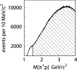
Figure 5: Distribution in the $\pi^{+}p$ effective mass for events in the charged mode satisfying the initial cuts. The shaded distribution shows the events accepted by the $m_{\pi^{+}p}>1.5$ GeV/$c^{2}$ requirement.

After all cuts are imposed 3.0M events remain in the neutral mode and 2.6M events remain in the charged mode. The resulting missing mass squared distribution (before the kinematic fit) is shown in the shaded distributions of Figure 3.

II.3 Effective mass and $t$ distributions

II.3.1 Uncorrected distributions

Distributions of the square of the four-momentum transfer, $t$, from the incoming $\pi^{-}$ to the outgoing $(3\pi)^{-}$ system as well as the $3\pi$ and $2\pi$ effective mass distributions are presented in Figures 6 and 7 for the events passing the cuts listed in Tables 1 and 2. These distributions have not been corrected for acceptance. The distribution in $t$ for the neutral mode is shown in Figure 6(a). The partial wave analysis, discussed below, was carried out for 12 bins in $t$ defined in Table 3. The $\pi^{-}\pi^{0}\pi^{0}$ effective mass distribution is shown in Figure 6(b). A peak at the $a_{2}(1320)$ is observed as well as an enhancement in the vicinity of the $\pi_{2}(1670)$. The $\pi^{-}\pi^{0}$ mass distribution in Figure 6(c) shows clear indication of the $\rho(770)$ and the $\pi^{0}\pi^{0}$ in Figure 6(d) shows the $f_{2}(1275)$.

The distribution in $t$ for the charged mode is shown in Figure 7(a). The $\pi^{-}\pi^{-}\pi^{+}$ effective mass distribution is shown in Figure 7(b). Peaks at the $a_{2}(1320)$ and $\pi_{2}(1670)$ are clearly observed. The $\pi^{-}\pi^{-}$ mass distribution in Figure 7(c) is featureless and the $\pi^{-}\pi^{+}$ in Figure 7(d) shows the $\rho(770)$ and the $f_{2}(1275)$.

Figure 6: (a) Uncorrected distribution in the square of the four-momentum transfer, $t$, from the incoming $\pi^{-}$ to the outgoing $(3\pi)^{-}$; (b) $(3\pi)^{-}$ effective mass distribution; (c) $\pi^{-}\pi^{0}$ effective mass distribution; and (d) $\pi^{0}\pi^{0}$ effective mass distribution for the neutral mode.

Figure 7: (a) Uncorrected distribution in the square of the four-momentum transfer, $t$, from the incoming $\pi^{-}$ to the outgoing $(3\pi)^{-}$; (b) $(3\pi)^{-}$ effective mass distribution; (c) $\pi^{-}\pi^{-}$ effective mass distribution; and (d) $\pi^{-}\pi^{+}$ effective mass distribution for the charged mode.

Table 3: Definition of the bins in $t$ – square of the four-momentum transferred from the incoming $\pi^{-}$ to the outgoing $(3\pi)^{-}$ system – used in this analysis.

$t$-Bin	Range in (GeV/$c$)2
$t1$	0.08 to 0.10
$t2$	0.10 to 0.12
$t3$	0.12 to 0.14
$t4$	0.14 to 0.16
$t5$	0.16 to 0.18
$t6$	0.18 to 0.23
$t7$	0.23 to 0.28
$t8$	0.28 to 0.33
$t9$	0.33 to 0.38
$t10$	0.38 to 0.43
$t11$	0.43 to 0.48
$t12$	0.48 to 0.53

Figure 8(a) shows the $\pi^{-}\pi^{0}\pi^{0}$ effective mass distribution for three regions of $t$ that we label $t1$, $t6$ and $t8$ and define in Table 3. Figure 8(b) shows the $\pi^{-}\pi^{-}\pi^{+}$ effective mass distribution for the same three regions of $t$. Clearly the overall shape of the $3\pi$ effective mass spectra strongly depends on $t$. These mass spectra are not corrected for acceptance.

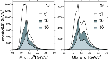
Figure 8: Uncorrected $(3\pi)^{-}$ mass distribution for the (a) neutral mode and (b) charged mode for three $t$ regions: $t_{1}$, $t_{6}$ and $t_{8}$ as defined in Table 3.

The various $2\pi$ effective mass spectra also depend on $3\pi$ mass. In Figure 9 we show several $2\pi$ spectra with the requirement that the $3\pi$ mass lie in the $a_{2}(1320)$ mass region ($1.20<m_{3\pi}<1.44$ GeV/$c^{2}$) or in the $\pi_{2}(1670)$ region ($1.54<m_{3\pi}<1.80$ GeV/$c^{2}$). The $\pi^{-}\pi^{0}$ mass spectrum (Figure 9(a)) and $\pi^{-}\pi^{+}$ mass spectrum (Figure 9(c)) are both dominated by the $\rho(770)$ when the $3\pi$ mass is in the $a_{2}$ region. The $\pi^{0}\pi^{0}$ mass spectrum (Figure 9(b)) and $\pi^{-}\pi^{+}$ mass spectrum (Figure 9(d)) both show strong signals for the $f_{2}(1270)$ when the $3\pi$ mass is in the $\pi_{2}$ region with the $\pi^{-}\pi^{+}$ mass spectrum also showing a $\rho(770)$ resonance signal.

Figure 9: Uncorrected $2\pi$ mass distributions for selected regions of the $3\pi$ effective mass. (a) $\pi^{-}\pi^{0}$ mass in the $a_{2}$ region; (b) $\pi^{0}\pi^{0}$ mass in the $\pi_{2}$ region; (c) $\pi^{-}\pi^{+}$ mass in the $a_{2}$ region; and (d) $\pi^{-}\pi^{+}$ mass in the $\pi_{2}$ region.

II.3.2 Mass and $t$ acceptance and resolution

The dependence of the experimental acceptance on relevant kinematic variables was estimated by generating Monte Carlo events for the two modes. Events were generated with an exponentially damped distribution in $t$, based on what is observed in the data. The generated distribution in $3\pi$ mass was uniform from $3m_{\pi}$ to 2.5 GeV/$c^{2}$. The $2\pi$ masses were chosen to uniformly populate the $3\pi$ Dalitz plot at fixed $3\pi$ mass and the distributions in the relevant decay angles were also generated uniformly.

The response of each detector component to a charged pion or photon from $\pi^{0}$ decay was simulated along with relevant smearing of momenta or energies. The detector responses were used as input to the same software used to reconstruct tracks and photons from actual data. The output was then passed on to the kinematic fitting software. The cuts summarized in Tables 1 and 2 were then imposed on the simulated event samples.

The acceptance as a function of $3\pi$ effective mass, for both neutral and charged modes, is shown in Figure 10(a). The acceptance as a function of $t$ for both modes is shown in Figure 10(b). The mass resolution, $\delta m$, as a function of $3\pi$ effective mass and $t$ resolution, $\delta t$, as a function of $t$ for both modes is shown in Figure 10(c) and 10(d) respectively.

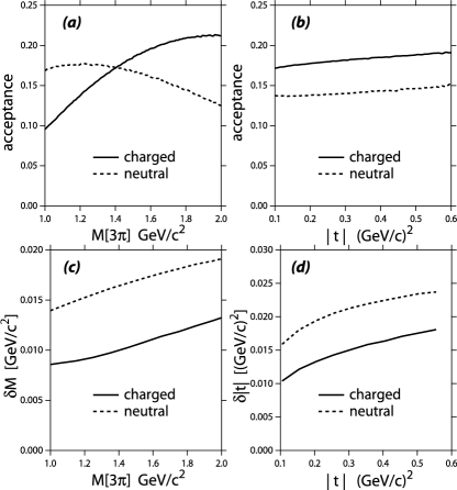
Figure 10: (a) $3\pi$ mass acceptance as a function of $3\pi$ mass; (b) $t$ acceptance as a function of $t$; (c) $\delta m$ – mass resolution as a function of $3\pi$ mass; and (c) $\delta t$ – $t$ resolution as a function of $t$ mass – all for both neutral and charged modes.

Figures 11(a) and 11(b) show the comparison between the acceptance-corrected $\pi^{-}\pi^{0}\pi^{0}$ and $\pi^{-}\pi^{-}\pi^{+}$ mass distributions for two regions in $t$, $t1$ and $t8$ (defined in Table 3).

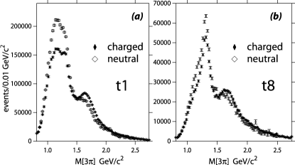
Figure 11: Acceptance corrected $\pi^{-}\pi^{0}\pi^{0}$ and $\pi^{-}\pi^{-}\pi^{+}$ effective mass distributions for two regions in $t$: (a) $t1$ and (b) $t8$. These $t$ regions are defined in Table 3.

III PWA methodology

III.1 Overview

The production of the $(3\pi)^{-}$ system in the reaction $\pi^{-}p\to(3\pi)^{-}p$ is described as a coherent and incoherent sum of partial wave amplitudes. The production through one such partial wave amplitude, assuming the isobar model, is shown schematically in Figure 12. The state $X$ described by the partial wave decays at point 1 into a di-pion resonance $R_{\pi\pi}$ (also referred to as the isobar) and a bachelor $\pi$ followed by the decay of the di-pion resonance at point 2 into $\pi_{a}$ and $\pi_{b}$. The state $X$ is characterized by $J^{PC}M^{\varepsilon}(SL)$, where $J$, $P$ and $C$ are the spin, parity and charge conjugation of the $3\pi$ system, respectively, $M$ is the spin projection along the $z$ axis and $\varepsilon$ represents symmetry (reflectivity) of the $3\pi$ system under reflection in the production plane. Viewed in terms of some exchange mechanism (as in Figure 12) $\varepsilon=+$ corresponds to natural parity exchange and $\varepsilon=-$ corresponds to unnatural parity exchange.

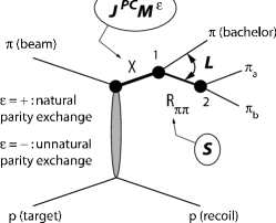
Figure 12: Partial wave analysis of the $3\pi$ system in the isobar model. The state $X$ is characterized by spin ($J$), parity ($P$) and charge conjugation ($C$). It decays at point 1 into a di-pion resonance $R_{\pi\pi}$ (the isobar) and a bachelor $\pi$. The di-pion has spin $S$. The angular momentum between the isobar and the bachelor $\pi$ is $L$. At point 2 the di-pion resonance decays into $\pi_{a}$ and $\pi_{b}$. More details are given in the text.

The decay at point 1 is described in the Gottfried-Jackson frame GJ which is the rest frame of the $3\pi$ system with the beam direction defining the $z$-axis and the normal to the production plane (specified by the momentum vectors of the beam and recoil proton) defining the $y$-axis. In this frame the angles of the bachelor pion are denoted by $\theta_{GJ}$ and $\phi_{GJ}$. The angular momentum between the bachelor pion and $R_{\pi\pi}$ is $L$, and the spin of $R_{\pi\pi}$ is $S$. The decay at point 2 ($R_{\pi\pi}\to\pi_{a}\pi_{b}$) is described in the helicity frame – the rest frame of the $\pi_{a}\pi_{b}$ system with the boost direction to that frame defining the $z$-axis. In this frame the angles of one of the decay pions is denoted by $\theta_{H}$ and $\phi_{H}$. The angular distributions for the isobar decay are given by the spin of $R_{\pi\pi}$ and the line shape as a function of $m_{\pi\pi}$ by a relativistic Breit-Wigner function with a Blatt-Weisskopf factor Chung02 with resonance parameters given by the Particle Data Group PDG . In this analysis the $S$-wave $\pi\pi$ isobars are parameterized according to the prescription described in reference Chung02 .

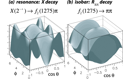
Figure 13: The decay angular structure for a particular partial wave where the resonance ($X$) has $J^{PC}=2^{-+}$ and decays into $f_{2}(1275)\pi$ where the isobar is the $f_{2}(1275)$ and the angular momentum between the isobar and bachelor $\pi$ is $L=2$. (a) The correlation between the decay angles ($\theta_{GJ},\phi_{GJ}$) of the resonance in the Gottfried-Jackson frame and (b) The correlation between the decay angles ($\theta_{H},\phi_{H}$) of the isobar in the helicity frame.

Figure 13 shows the correlated angular decay structure between $\theta_{GJ},\phi_{GJ}$ and $\theta_{H},\phi_{H}$ for one particular partial wave corresponding to the decay of resonance $X$ with $J^{PC}=2^{-+}$ into $f_{2}(1275)\pi$ where the isobar is the $f_{2}(1275)$ and the angular momentum between the isobar and bachelor $\pi$ is $L=2$. A typical PWA involved fitting coherent or incoherent sums of many such correlated distributions to the observed data, while taking into account the acceptance of the experiment. The acceptance in the relevant decay angles for the $3\pi$ effective mass in the $\pi_{2}(1670)$ mass region is shown in Figure 14.

Figure 14: The acceptance in decay angles for the $3\pi$ effective mass in the $\pi_{2}(1670)$ mass region. The angles $\theta$ and $\phi$ are measured in the Gottfried-Jackson frame for the resonance decay and in the helicity frame for the isobar decay. Acceptances are shown for (a) $\cos\theta$ and (b) $\phi$ for both the charged and neutral modes of the $3\pi$ system.

The observed intensity as a function of $m_{3\pi}$ and $t$ is written as:

$$I(m_{3\pi},t,\tau)=\eta(\tau)\sum_{\varepsilon}\left|\sum_{b}a_{b}^{\varepsilon}(m_{3\pi},t)A_{b}^{\varepsilon}(\tau)\right|^{2}$$ (1)

where $a_{b}^{\varepsilon}(m_{3\pi},t)$ is the production amplitude, $A_{b}^{\varepsilon}(\tau)$ is the decay amplitude and $\tau=\{\theta_{GJ},\phi_{GJ},\theta_{H},\phi_{H},m_{\pi\pi}\}$ is the set of kinematic variables describing the decay of the resonance and isobar. The index $b$ enumerates the spin variables of the partial wave and $\varepsilon$ the reflectivity, as defined below. The $A_{b}^{\varepsilon}(\tau)$ involve products of $D^{J\star}_{M\lambda}$ functions for the two decays and a function describing the line shape of the isobar. In detail:

$$A_{JML}(\tau)= \sqrt{(2L+1)(2S+1)}$$

$$\times\sum_{\lambda}D^{J\star}_{M\lambda}(\theta_{GJ},\phi_{GJ},0)D^{S\star}_{\lambda 0}(\theta_{H},\phi_{H},0)$$

$$\times\langle L0S\lambda|J\lambda\rangle$$

$$\times F_{L}(p_{X})F_{S}(p_{R})BW(m_{\pi\pi})+(1\to 2)$$

where $1,2$ refer to the two identical pions ($\pi^{-}$’s in the charged mode and $\pi^{0}$’s in the neutral), $J,M$ are the spin and projection of the resonance, $S$ is the spin of the isobar and $L$ is the orbital angular momentum between the isobar and the bachelor pion. The functions $F_{L}(p_{X})$ and $F_{S}(p_{R})$ are the barrier factors as a function of the breakup momentum, $p_{X}$ and $p_{R}$, for $X$ and the isobar respectively. $BW(m_{\pi\pi})$ is the Breit Wigner function for the isobar. In the reflectivity basis:

$$A_{JML}^{\varepsilon}=\Theta(M)\left[A_{JML}-\varepsilon P(-1)^{J-M}A_{J-ML}\right]$$ (3)

where $P$ is the parity of the resonance, $\Theta(0)=1/2$, $\Theta(M>0)=\sqrt{1/2}$ and $\Theta(M<0)=0$.

The goal of the PWA is to extract the production amplitudes by fitting the correlated decay angular distributions to the intensity described by equation 1 in bins of $m_{3\pi}$ and $t$. In order to account for detector acceptance, Monte Carlo simulations were used to find the acceptance function $\eta(\tau)$ in terms of the set of kinematic variables $\tau$. Thus the data were fitted to the decay amplitudes modified by the acceptance function.

The PWA formalism used here is identical to that used in Chung02 and Chung93 and is also briefly described in internal notes 3piE852 . The PWA software was developed at Brookhaven Lab and Indiana University (IU) 3piE852 . The IU software was optimized for running on a 200-processor computer cluster (AVIDD) AVIDD allowing systematic studies involving many PWA fits, varying isobar parameters and using different wave sets. The IU programs were also used to analyze the data presented in Chung02 and produced consistent results (see Appendix A for a list of technical notes available online).

III.2 Selecting a partial wave set

III.2.1 General criteria

As noted earlier, it is important to include in the analysis a set of partial waves sufficient to describe the physics and to have well understood criteria for selecting this set. One technique, following Daum81 , is to start with some parent set of waves and examining the change in likelihood resulting from sequentially removing waves.

Table 4: Partial waves under consideration in this analysis.

$J^{PC}M^{\varepsilon}$	$L$	Isobar $\pi$	Wave Set
$0^{-+}0^{+}$	S	$(\pi\pi)_{S}\pi$	B
$0^{-+}0^{+}$	S	$f_{0}\pi$	B
$0^{-+}0^{+}$	P	$\rho\pi$	B
$1^{++}0^{+}$	S	$\rho\pi$	B
$1^{++}1^{+}$	S	$\rho\pi$	B
$1^{++}1^{-}$	S	$\rho\pi$	L
$1^{++}0^{+}$	P	$f_{0}\pi$	H
$1^{++}0^{+}$	P	$(\pi\pi)_{S}\pi$	H
$1^{++}1^{+}$	P	$f_{2}\pi$	H
$1^{++}0^{+}$	D	$\rho\pi$	L
$1^{-+}1^{+}$	P	$\rho\pi$	B
$1^{-+}0^{-}$	P	$\rho\pi$	B
$1^{-+}1^{-}$	P	$\rho\pi$	B
$2^{++}1^{+}$	D	$\rho\pi$	B
$2^{++}0^{-}$	D	$\rho\pi$	B
$2^{-+}0^{+}$	S	$f_{2}\pi$	B
$2^{-+}1^{+}$	S	$f_{2}\pi$	B
$2^{-+}1^{-}$	S	$f_{2}\pi$	L
$2^{-+}0^{+}$	P	$\rho\pi$	B
$2^{-+}1^{+}$	P	$\rho\pi$	H
$2^{-+}0^{+}$	P	$\rho_{3}\pi$	H
$2^{-+}1^{+}$	P	$\rho_{3}\pi$	H
$2^{-+}0^{+}$	D	$(\pi\pi)_{S}\pi$	B
$2^{-+}0^{+}$	D	$f_{0}\pi$	H
$2^{-+}1^{+}$	D	$(\pi\pi)_{S}\pi$	H
$2^{-+}1^{+}$	D	$f_{0}\pi$	H
$2^{-+}1^{+}$	D	$f_{2}\pi$	B
$2^{-+}0^{+}$	D	$f_{2}\pi$	B
$2^{-+}0^{+}$	F	$\rho\pi$	H
$2^{-+}1^{+}$	F	$\rho\pi$	H
$3^{++}0^{+}$	S	$\rho_{3}\pi$	B
$3^{++}0^{+}$	P	$f_{2}\pi$	H
$3^{++}0^{+}$	D	$\rho\pi$	H
$4^{++}0^{+}$	D	$\rho_{3}\pi$	H
$4^{++}0^{+}$	F	$f_{2}\pi$	H
$4^{++}0^{+}$	G	$\rho\pi$	H
$4^{-+}0^{+}$	P	$\rho_{3}\pi$	H
$4^{-+}0^{+}$	F	$\rho\pi$	H
Background			B

Another arbiter of wave set sufficiency is the comparison of moments, $H(\ell mm^{\prime})$, of the $D^{\ell}_{mm^{\prime}}(\Omega)$ functions as calculated directly from the data and as calculated using the results of PWA fits. A PWA using a sufficient set of partial waves will reproduce all angular distributions of the data as evidenced by the agreement of the observed and calculated moments. We define $H(\ell mm^{\prime})=\int I(\Omega)D^{\ell}_{mm^{\prime}}(\Omega)d\Omega$ where $\Omega$ represents the Euler angles of the $3\pi$ system and the intensity $I(\Omega)$ is determined directly from experiment or computed using the results of the PWA fits. Both of these techniques were used in this analysis.

III.2.2 Defining a parent set of waves

The $\pi\pi$ isobars included in this analysis are the $\sigma$, $f_{0}(980)$, $\rho(770)$, $f_{2}(1275)$ and $\rho_{3}(1690)$ where $\sigma$ is meant to indicate a $S$-wave $\pi\pi$ system as described in Chung02 . In addition, a background wave is included. The background wave is characterized by a uniform distribution in the relevant decay angles and is added incoherently with the other waves. We restrict the parent wave set to those with $J\leq 4$, $M\leq 1$ and $S\leq 3$.

III.2.3 Removing waves from the parent set

Waves were sequentially removed from the parent set and the resulting change in likelihood ($\cal{L}$) examined 3piE852 . Three passes were used. First, waves with an L=0 isobar ($\pi\pi$ $S$-wave and $f_{0}$) were examined. Subsequent passes examined $L=2$ ($f_{2}$) and $L=1$ ($\rho$) isobar partial waves. A PWA with the wave in question removed was performed and the resulting likelihood compared to PWA including the wave. If the change in $\ln\cal{L}$ was less than 40 the wave was removed. Figure 15 shows the change in $\ln\cal{L}$ when a significant, but not a dominant, wave ($2^{-+}1^{+}f_{2}\pi D\$wave) is removed compared to when an insignificant wave ($2^{-+}1^{-}f_{2}\pi\ D\$wave) is removed.

Certain partial waves that would have been removed by this selection criterion were kept because the existence of signals in these waves is under consideration. The negative reflectivity exotic $1^{-+}$ partial waves were kept even though they would have been chosen for removal by the above criterion. The positive reflectivity exotic partial wave failed the selection criterion everywhere above 1.4 ${\rm{GeV}}/c^{2}$ and exhibited large fluctuations in intensity below this mass. This partial wave was also kept and its contribution to the likelihood is further examined below using the final set of partial waves. Finally, the $2^{++}0^{-}\rho\pi\ D$-wave (which failed the selection test) was kept to serve as a possible reference wave for evaluation of phase differences of negative reflectivity partial waves. Based on these criteria the compiled set includes 35 waves and a background wave. We refer to this as the high-wave set.

The analysis reported in reference Chung02 used a wave set consisting of 20 waves including the background wave – we refer to this as the low-wave set. Table 4 lists the waves used in low-wave and high-wave sets. The waves included only in the low-wave set are labeled with [L] in Table 4 while the waves included only in the high-wave set are labeled with [H] and those included in both sets are labeled with [B].

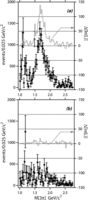
Figure 15: Partial wave intensity (filled circles) as a function of $3\pi$ mass (lower plot) shown along with the change in $\ln\cal{L}$ (shown above the intensity plot – read the right axis scale) that results when this partial wave is removed from the parent set of partial waves. (a) $2^{-+}1^{+}f_{2}\pi D\$wave - a significant wave and (b) $2^{-+}1^{-}f_{2}\pi D\$wave - an insignificant wave.

III.2.4 Using moments

The PWA solutions obtained with the two wave sets were used to compute moments that were then compared directly with data. In Figure 16 we show the $H(201)$ and $H(420)$ moment comparisons as a function of $3\pi$ mass for the $\pi^{-}\pi^{0}\pi^{0}$ mode for low-wave and high-wave set PWA fits. We also show the difference between data and PWA calculations of the moments as $\Delta^{2}$ (summing differences squared divided by errors squared summed over all mass bins and divided by the number of mass bins) for various moments. Similar plots are shown in Figure 17 for the $\pi^{-}\pi^{-}\pi^{+}$ mode. The moments calculated using the PWA results from the high wave set have better agreement with experimental moments, but there are moments (such as $H(201)$ - shown in part (a) of Figure 17) for which agreement is not achieved. This may be due to the inherent inadequacy of the isobar model in describing the underlying production mechanism.

An examination of Figures 16(c) and 17(c) show that for all the moments, the moments calculated using the high-wave set have better agreement with data than do moments calculated using the low-wave set.

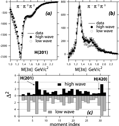
Figure 16: Comparison of the (a) H(201) and (b) H(420) moments as computed directly from data and from PWA fits for the low and high wave sets for the $\pi^{-}\pi^{0}\pi^{0}$ channel. In (c) the $\Delta^{2}$ (differences squared divided by errors squared summed over all mass bins and divided by the number of mass bins) is shown for various moments.

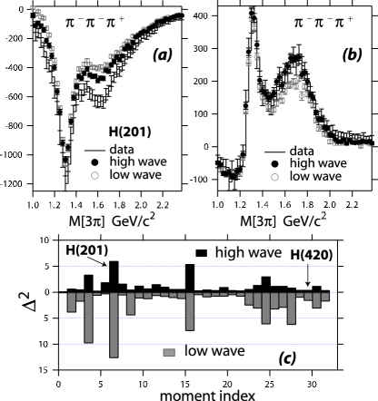
Figure 17: Comparison of the (a) H(201) and (b) H(420) moments as computed directly from data and from PWA fits for the low and high wave sets for the $\pi^{-}\pi^{-}\pi^{+}$ channel. In (c) the $\Delta^{2}$ (differences squared divided by errors squared summed over all mass bins and divided by the number of mass bins) is shown for various moments.

IV PWA results

The PWA results presented in this section were for data with $0.18<|t|<0.23$ (GeV/$c$)² referred to as $t6$ in Table 3. The analysis was also carried out in 11 other bins in $|t|$ – some results of which will also be summarized below.

Figure 18 shows the sum of all waves in the high-wave set along with the background wave for both the charged and neutral modes. The fitting procedure constrains the sum of all the waves to agree with the acceptance-corrected $3\pi$ mass distribution. The background wave (uniform in all angles) is added incoherently with the other waves. As can be seen, the contribution from the background wave is small (of order 1%).

There is a systematic disagreement in the relative normalization between the two modes resulting from an overall per track inefficiency of 5% in the trigger PWC’s. The overall inefficiency has no bearing on the features of the acceptances and was thus not incorporated into the Monte Carlo corrections, but results in the neutral mode having a yield consistently 25% higher than the charged mode. The neutral mode required only one forward-going charged particle in the trigger while the charged mode required three.

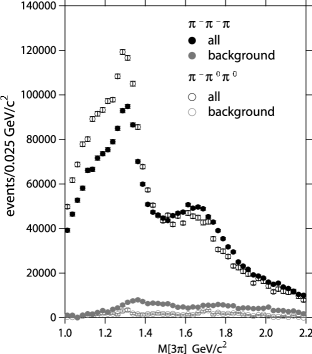
Figure 18: The sum of a partial waves and the background wave for both the charged and neutral modes.

In the following we discuss intensities and phases of individual partial waves. A partial wave intensity corresponds to a single term of equation (1) which is a product of the fitted partial wave amplitude, $a^{\epsilon}_{b}(m_{3\pi},t)$, and the isobar amplitude $A_{JML}(\tau)$ . Similar to the procedure followed in references Adams98 ; Chung02 , the intensities are integrated over acceptance corrected data, and are normalized to the total number of events.

The coherent sum of the $1^{++}$ $\rho\pi$-waves is shown in Figure 19 for the $\pi^{-}\pi^{-}\pi^{+}$ and $\pi^{-}\pi^{0}\pi^{0}$ modes. For each the results from the high wave set and low wave set are shown. The $1^{++}$ wave is a dominant wave and the results of the PWA for the two wave sets (high and low) are in good agreement. The yield for the two charged modes is also consistent with expectations from isospin for the $\rho\pi$ system.

The $1^{++}$ $\rho\pi$ $D$-wave is not included in the high-wave set, since it did not meet criteria for inclusion, but it is included in the low-wave set. The observed ratio of $1^{++}$ $\rho\pi$ $S$-wave to $D$-wave in the low-wave set is consistent with that of reference Chung02 .

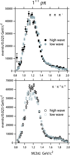
Figure 19: Coherent sum of the $1^{++}$ $\rho\pi$-waves for the (upper) $\pi^{-}\pi^{-}\pi^{+}$ and (lower) $\pi^{-}\pi^{0}\pi^{0}$ modes. For each the results from the high wave set and low wave set are shown.

Figure 20 shows the $2^{++}1^{+}\ D$-wave $\rho\pi$ partial wave as a function of $m_{3\pi}$ for both the neutral and charged modes. A clear $a_{2}(1320)$ signal is observed. For a pure $\rho\pi$ isovector resonance, we expect an equal number of charged mode and neutral mode events. This wave is clean and robust and will be used for interferometry to study the phase motion of other waves relative to this wave.

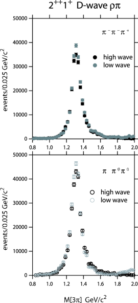
Figure 20: $2^{++}1^{+}\ D$-wave $\rho\pi$ partial wave intensity for the (upper) $\pi^{-}\pi^{-}\pi^{+}$ and (lower) $\pi^{-}\pi^{0}\pi^{0}$ modes. For each the results from the high wave set and low wave set are shown.

Figures 21 and 22 show the intensities for the $2^{-+}0^{+}\ S$-wave $f_{2}\pi$ and $2^{-+}0^{+}\ D$-wave $f_{2}\pi$ waves respectively for both the charged and neutral modes. Note that the relative yields between charged and neutral modes, for these $f_{2}\pi$ decays are consistent with expectations from isospin, after taking into account the overall 25% reduction in yield for the charged mode. These intensities are also compared with those measured by Daum et. al. Daum81 in a similar amplitude analysis of diffractive $3\pi$ production in $\pi^{-}p$ interactions at 63 and 94 GeV/$c^{2}$. The Daum results have been arbitrarily scaled by a factor of 5.

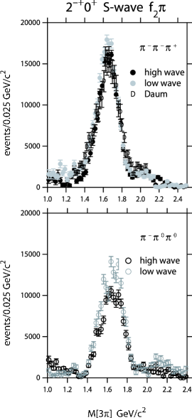
Figure 21: $2^{-+}0^{+}\ S$-wave $f_{2}\pi$ partial wave intensity for the (upper) $\pi^{-}\pi^{-}\pi^{+}$ and (lower) $\pi^{-}\pi^{0}\pi^{0}$ modes. For each the results from the high wave set and low wave set are shown.

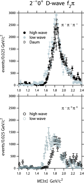
Figure 22: $2^{-+}0^{+}\ D$-wave $f_{2}\pi$ partial wave intensity for the (upper) $\pi^{-}\pi^{-}\pi^{+}$ and (lower) $\pi^{-}\pi^{0}\pi^{0}$ modes. For each the results from the high wave set and low wave set are shown.

The $S$ and $D$ $f_{2}\pi$ modes both show a resonant-like structure but not at the same peak position. The $S$ wave peaks at approximately 1.6 GeV/$c^{2}$ while the $D$ wave peaks at approximately 1.8 GeV/$c^{2}$. This shift in the peak position has been observed in other analyses Chung02 ; Daum81 . This has been interpreted as the $f_{2}\pi$ decay mode of two different resonances. The PDG places the $\pi_{2}(1670)$ $2^{-+}$ resonance at a mass of 1.67 GeV/$c^{2}$ based on fits to the $S$ wave mode alone.

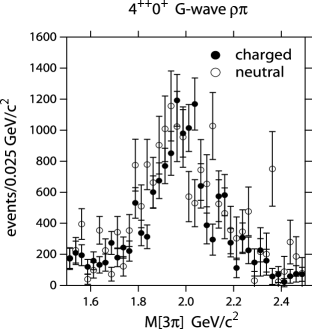
Figure 23: The $4^{++}0^{+}\ G$-wave $\rho\pi$ partial wave intensity for the $\pi^{-}\pi^{-}\pi^{+}$ and $\pi^{-}\pi^{0}\pi^{0}$ modes.

Figure 23 shows the $4^{++}0^{+}\ G$-wave $\rho\pi$ intensity as a function of $m_{3\pi}$ for both the neutral and charged modes. Comparing Figures 23 and 20 the yield of $a_{4}(2040)$ is about 3% that of the $a_{2}(1320)$ indicating the sensitivity of the PWA within the isobar model for finding states with relatively low production cross-sections.

V The exotic $1^{-+}$ wave

V.1 Comparing the high and low wave sets

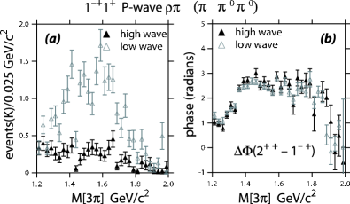
Figure 24: (a) The $1^{-+}1^{+}\ P$-wave $\rho\pi$ partial wave in the neutral mode ($\pi^{-}\pi^{0}\pi^{0}$) for the high-wave set PWA and the low-wave set PWA and (b) the phase difference $\Delta\Phi$ between the $2^{++}$ and $1^{-+}$ for the two wave sets.

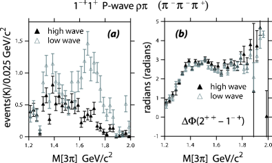
Figure 25: (a) The $1^{-+}1^{+}\ P$-wave $\rho\pi$ partial wave in the charged mode ($\pi^{-}\pi^{-}\pi^{+}$) for the high-wave set PWA and the low-wave set PWA and (b) the phase difference $\Delta\Phi$ between the $2^{++}$ and $1^{-+}$ for the two wave sets.

The $1^{-+}1^{+}\ P$-wave $\rho\pi$ partial wave and its interference with the $2^{++}$ wave are shown in parts (a) and (b) of Figures 24 and 25 for the neutral mode ($\pi^{-}\pi^{0}\pi^{0}$) and charged mode ($\pi^{-}\pi^{-}\pi^{+}$). When the low-wave set is used in the fit, an enhancement is observed for the exotic $1^{-+}$ wave in the $3\pi$ mass region around 1.6 GeV/$c^{2}$, consistent with the observation of Adams98 ; Chung02 . The enhancement disappears when the high wave set is used. This effect is observed for both $3\pi$ channels. The phase of the exotic wave relative to the dominant $2^{++}$ wave (see Figures 24(b) and 25(b)) is similar for both wave sets and dominated by the phase of the $a_{2}(1320)$. The apparent phase motion beginning around 1700 MeV/$c^{2}$ is likely due to the $a_{2}(1700)$ PDG , but the unreliability of the exotic intensity makes this an inappropriate place for its study.

V.2 Leakage of the $\pi_{2}(1670)$ and the instability of the exotic wave

One source of leakage into the exotic wave for the PWA carried out with the low-wave set is the $\pi_{2}(1670)$. In Figure 26 the coherent sum of the intensities for the $2^{-+}0^{+}\ F$-wave $\rho\pi$, $2^{-+}1^{+}\ F$-wave $\rho\pi$ and $2^{-+}1^{+}\ P$-wave $\rho\pi$ waves for the charged and neutral modes are shown. These waves are allowed decay modes of the $\pi_{2}(1670)$. A clear peak is seen at the $\pi_{2}(1670)$ mass, the same mass region where the purported exotic meson was seen using the low-wave set. The three waves shown in Figure 26 were not included in the low-wave set.

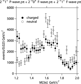
Figure 26: Sum of the intensities for the $2^{-+}0^{+}\ F$-wave $\rho\pi$, $2^{-+}1^{+}\ F$-wave $\rho\pi$ and $2^{-+}1^{+}\ P$-wave $\rho\pi$ waves for the charged and neutral modes. These waves were included in the high-wave set but not in the low-wave set.

The PWA fit was repeated for the high wave set but with the $2^{-+}0^{+}\ F$-wave $\rho\pi$, $2^{-+}1^{+}\ F$-wave $\rho\pi$ and $2^{-+}1^{+}\ P$-wave $\rho\pi$ waves removed. The resulting $1^{-+}\ P$-wave $\rho\pi$ intensities for the neutral mode for this modified high wave set fit, along with the unmodified high wave set and low wave set, are shown in Figures 27. The corresponding results for the charged mode are shown in Figure 28. The agreement between the modified high wave set and the low wave set shows that the $2^{-+}\ F$-wave $\rho\pi$ decays and the $2^{-+}1^{+}\ P$-wave $\rho\pi$ decay of the $\pi_{2}$ are the source of leakage leading to the observed exotic peak in the low wave set.

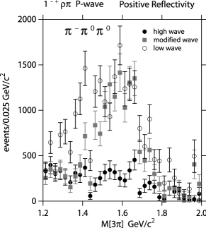
Figure 27: The positive reflectivity $1^{-+}\ P$-wave $\rho\pi$ intensity for the neutral mode for the high wave set (filled circles), the modified high wave set (filled squares) and the low wave set (open circles). In the modified high wave set the two $2^{-+}\ F$-wave $\rho\pi$ waves and the $2^{-+}1^{+}\ P$-wave $\rho\pi$ wave were removed.

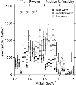
Figure 28: The positive reflectivity $1^{-+}\ P$-wave $\rho\pi$ intensity for the charged mode for the high wave set (filled circles), the modified high wave set (filled squares) and the low wave set (open circles). In the modified high wave set the two $2^{-+}\ F$-wave $\rho\pi$ waves and the $2^{-+}1^{+}\ P$-wave $\rho\pi$ wave were removed.

V.3 Evidence for leakage of the $a_{4}(2040)$

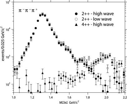
Figure 29: The $2^{++}$ intensity for charged $3\pi$ mode for the high wave set (filled circles) and low wave set (open circles). The $4^{++}$ intensity (filled triangles) for the high wave set is also shown.

A similar phenomenon is observed in the $2^{++}$ wave in the low wave set where the $4^{++}0^{+}\ G$-wave $\rho\pi$ is not included. As discussed above, the $4^{++}0^{+}\ G$-wave $\rho\pi$ in the high wave set clearly shows the $a_{4}(2040)$. Figure 29 shows a semi-log plot of the the $2^{++}$ intensity for charged $3\pi$ mode for the high wave set (filled circles) and low wave set (open circles). The $4^{++}$ intensity for the high wave set is also shown (filled triangles). The $a_{2}(1320)$ is dominant in the $2^{++}$ intensity in both high and low wave sets. The $2^{++}$ intensity for the low wave set shows a resonance-like structure near 2 GeV/$c^{2}$ in low wave set but not the high wave set. However the $2^{++}$ low wave set intensity agrees well with the $4^{++}$ high wave set intensity. In this case, leaving out the $4^{++}$ in the low wave set forces a enhancement at $\sim 2$ GeV/$c^{2}$ in the $2^{++}$ wave.

V.4 Further discussion of the significance of the exotic wave

The contribution to the $\ln{\cal{L}}$ of the positive reflectivity exotic partial wave was examined by removing this wave from the high wave set and comparing the resulting likelihood with that of the original high wave PWA. Figure 30 shows the resulting change in likelihood. The sign convention of this difference is such that positive (negative) values indicate inclusion of this partial wave improved (degraded) the fit quality. As can be seen from figure 30 there is no region of $3\pi$ effective mass where this partial wave is consistently required by the fit. This behavior is seen in all t-bins presented here.

Figure 30: The change in $\ln{\cal{L}}$ resulting from the removal of the $1^{-+}1^{+}(\rho\pi)$P-wave partial wave. See the text for the sign convention and discussion.

V.5 $t$ dependence studies

V.5.1 The exotic wave

Figure 31: Variation of the $1^{-+}1^{+}\ P$-wave $\rho\pi$ intensity for the charged mode for the 12 $t$-bins of Table 3 increasing in $|t|$ from left to right and top to bottom.

Figure 32: Variation of the $2^{-+}0^{+}\ S$-wave $f_{2}\pi$ intensity for the charged mode for the 12 $t$-bins of Table 3, increasing in $|t|$ from left to right and top to bottom.

Figure 33: Variation of the phase difference between the $1^{-+}$ and $2^{-+}$ amplitudes, whose intensities are shown in Figures 31 and 32 respectively, for the charged mode for the 12 $t$-bins of Table 3, increasing in $|t|$ from left to right and top to bottom.

Figure 34: Variation of the $2^{++}1^{+}\ D$-wave $\rho\pi$ intensity for the charged mode for the 12 $t$-bins of Table 3, increasing in $|t|$ from left to right and top to bottom.

Figure 35: Variation of the $4^{++}0^{+}\ G$-wave $\rho\pi$ intensity for the charged mode for the 12 $t$-bins of Table 3, increasing in $|t|$ from left to right and top to bottom.

We examined the stability of the exotic wave intensity and the intensity of other waves across the 12 $t$-bins shown in Table 3 for the high wave fit in the charged $3\pi$. As noted in Table 3, the width of the $|t|$ bin for the first five bins is 0.02 (GeV/$c$)² and 0.05 (GeV/$c$)² for the other bins. Figures 31, 32 and 33 show the variation of the $1^{-+}1^{+}\ P$-wave $\rho\pi$ intensity, the $2^{-+}0^{+}\ S$-wave $f_{2}\pi$ intensity and the phase difference between the $1^{-+}$ and $2^{-+}$ amplitudes for the charged $3\pi$ mode for the 12 $t$-bins. The $2^{-+}0^{+}\ S$-wave $f_{2}\pi$ intensity is stable across the 12 $t$ bins. We note that although the $1^{-+}1^{+}\ P$-wave $\rho\pi$ intensity may indicate an enhancement in the vicinity of $\sim 1.6$ GeV/$c^{2}$ for some of the higher $t$ bins in Figure 31, the corresponding phase difference shown in Figure 33 is not consistent with resonant behavior. Indeed the $2^{-+}0^{+}\ S$-wave $f_{2}\pi$ and $1^{-+}1^{+}\ P$-wave $\rho\pi$ are phase-locked in the 1.6 GeV/$c^{2}$ region. One possible explanation is production of an exotic resonance with the same mass, width and phase motion as the $\pi_{2}(1670)$. Another is some residual leakage of the $\pi_{2}(1670)$ in the exotic wave in the high-wave set.

V.5.2 The $2^{++}$ and $4^{++}$ waves

The $2^{++}1^{+}\ D$-wave $\rho\pi$ intensity (shown in Figure 34) and the $4^{++}0^{+}\ G$-wave $\rho\pi$ intensity (shown in Figure 35) are shown for the 12 $t$ bins. For completeness, in Figure 36, we compare the $t$ dependence of the $2^{++}1^{+}\ D$-wave $\rho\pi$ intensity, dominated by the $a_{2}(1320)$, in both $3\pi$ modes in this experiment, with other measurements of $\pi^{-}p\to a_{2}^{-}(1320)p$ at 18.8 GeV/$c$Chabaud .

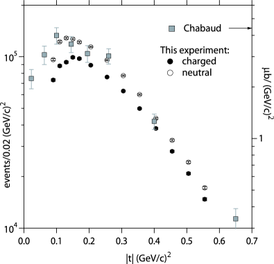
Figure 36: $t$ dependence of the $a_{2}(1320)$ as measured in this experiment for the charged mode (filled circles) and neutral mode (open circles) along with measurements of V. Chabaud et. al. Chabaud of $\pi^{-}p\to a_{2}^{-}(1320)p$ at 18.8 GeV/$c$.

VI Studies of systematics

VI.1 Effects of varying data selection cuts

Studies were carried out to determine the effect on the PWA of varying the parameters that define the selection criteria as described in section II.2. Different criteria were found to effect the results in different ways but no significant change in our conclusions was observed. The effects of these perturbations on the analysis are described individually below.

The beam hole cut is nominally $2.5\sigma$. Values of $1.5\sigma$ and $3.5\sigma$ systematically increased and decreased the intensity of the $1^{++}\rho\pi$ $S$-wave below 1.2 GeV/$c^{2}$ but left the mass region above 1.2 GeV$/c^{2}$ indistinguishable from the unperturbed analysis. The changes observed were approximately 5% of the intensity. Conclusions regarding the low mass behavior of this partial wave should take into account this systematic effect. Other partial waves were unaffected.

The cut to remove the $\Delta^{++}$ in the charged sample affected the data only above 2.0 GeV/$c^{2}$. Removing this cut from the analysis increased the intensity of the $2^{-+}0^{+}(f_{2}\pi)$ $S$-wave by approximately twice its error between 2.0 and 2.4 GeV/$c^{2}$. The systematic effect on other partial waves is insignificant when compared with their statistical errors.

The effect of removing the DEA cut was similar to using a less restrictive value for the beam hole cut. Small, but statistically significant, increases in the intensity of the $2^{-+}0^{+}(f_{2}\pi)$ $S$-wave were observed between 1.2 and 1.6 GeV/$c^{2}$.

Increasing (decreasing) the confidence level cut to 0.3 (0.1) changed the observed intensities everywhere by a mass independent scale factor. The same effect was observed for the CSI cut. Removing this cut increased all intensities by a factor of 1.66 but left their shapes unchanged.

In summary, we have investigated the effect of perturbing the selection criteria summarized in Tables 1 and 2 on the results of the partial wave fit and have shown that our results do not depend on the specific values used in the criteria.

VI.2 $S$-wave parametrization

We used the isobar model, following the same methodology employed in references Adams98 ; Chung02 . This model uses two-body amplitudes for the $\pi\pi$ system. The $S=1$ isovector and $S=2$ isoscalar amplitudes were parametrized using Breit-Wigner amplitudes. There are various $S=0$, isoscalar parametrizations available in the literature. In general the $\pi\pi$ amplitude is dominated by a broad $\sigma$ meson, the $f_{0}(980)$ and several resonances above $1\mbox{ GeV}/c^{2}$, depending on the specific parametrization. The results presented in this paper were all based on the parametrization used in references Adams98 ; Chung02 . This is based on the model of  AMP with the possibility of direct $f_{0}(980)$ production; the $f_{0}(980)$ was subtracted from the elastic $\pi\pi$ amplitude and added as a Breit-Wigner resonance. We have also studied other parametrizations, e.g. based on (1) $N/D$ dispersion relations, (2) explicit inclusions of the $K{\bar{K}}$ channel and/or (3) including direct production of scalar resonances above $1\mbox{ GeV}/c^{2}$ oset ; oset-nd . All give qualitatively identical results.

VII Conclusions

A partial wave analysis of the $\pi^{-}\pi^{-}\pi^{+}$ and $\pi^{-}\pi^{0}\pi^{0}$ systems has been presented using a data set whose statistics exceeds published analyses of the $3\pi$ systems. The $a_{1}(1260)$, $a_{2}(1320)$, $\pi_{2}(1670)$ and $a_{4}(2040)$ mesons were observed. The data provide no evidence for an exotic $J^{PC}=1^{-+}$ meson as had been reported earlier using a smaller sample of the $\pi^{-}\pi^{-}\pi^{+}$ mode alone Adams98 ; Chung02 . This analysis included the study of criteria for defining a set of partial waves sufficient to describe the data including a study of the effect on the fit quality by removing individual waves and also a comparison of observed moments of the data with moments computed from PWA solutions. The wave set thus established contained more waves than were used in the analysis reporting evidence for the exotic meson. Our studies indicate that leaving out partial waves corresponding to decay modes of the $\pi_{2}(1670)$ lead to a false enhancement in the exotic $1^{-+}$ wave. This analysis and the analysis of references Adams98 ; Chung02 were based on the isobar model. The isobar model is known to suffer some limitations, as has been pointed by others Ascoli73; Ascoli74 . The so-called Deck mechanism Ascoli73; Ascoli74 is particularly relevant to the production of the $3\pi$ system and is being applied to these data. Results will be presented in a forthcoming paper.

Appendix A Technical notes and online PWA results

The authors of this paper have made available technical notes and PWA results online 3piE852 . The notes include (1) details of the data selection; (2) a comparison of the software used in this analysis with that used in the analysis of reference Chung02 ; (3) the Monte Carlo details for this analysis; (4) a full description of the PWA formalism; (5) the moments method technique and definition of angles; (6) a study of background contributions to partial wave intensities; (7)  stability of PWA results against variations in data selection criteria; (8)  acceptance and resolution; (9) the determination of the minimal partial wave set and (10) $S$-wave parametrization. In addition, PWA results (amplitudes and phases) are available for 12 bins in $t$ and for various wave sets.

References

- (1) J. Ballam et. al. Phys. Rev. Lett. 21, 934 (1968).
- (2) G. Ascoli et. al. Phys. Rev. Lett. 25, 962 (1970).
- (3) Yu. Antipov et. al. Nucl. Phys. B63, 141 (1973).
- (4) C. Baltay et. al. Phys. Rev. Lett. 39, 591 (1977).
- (5) C. Daum et. al. (ACCMOR Collaboration), Phys. Lett. B 89, 276 (1980).
- (6) C. Daum et. al. (ACCMOR Collaboration), Phys. Lett. B 89, 281 (1980).
- (7) C. Daum et. al. (ACCMOR Collaboration), Phys. Lett. B 89, 285 (1980).
- (8) C. Daum et. al. (ACCMOR Collaboration), Nucl. Phys, B182,269 (1981).
- (9) G. S. Adams et. al. Phys. Rev. Lett. 81, 5760 (1998).
- (10) S. U. Chung et. al. Phys. Rev. D65, 072001 (2002).
- (11) G. S. Bali and A. Pineda Phys. Rev. D69, 094001 (2004).
- (12) S. Teige et. al. Phys. Rev. D59, 012001 (1999).
- (13) Z. Bar-yam et. al. Nucl. Intrum. Methods Phys. Res. A 386, 235 (1997).
- (14) T. Adams et. al. Nucl. Intrum. Methods Phys. Res. A 368, 617 (1996).
- (15) B. Brabson et. al. Nucl. Intrum. Methods Phys. Res. A 322, 419 (1993).
- (16) R. Crittenden et. al. Nucl. Intrum. Methods Phys. Res. A 387, 377 (1997).
- (17) J. Gunter, Ph. D. Thesis, Indiana University (1997).
- (18) R. Lindenbusch, Ph. D. Thesis, Indiana University (1997).
- (19) A. R. Dzierba et. al. The authors of this paper have posted notes on the web regarding the 3 data processing and selection, PWA formalism, software and other details. URL: dustbunny.physics.indiana.edu/3pi_paper (2005).
- (20) O. Dahl et. al., SQUAW kinematic fitting program, Group A programming note P-126, U. California Berkeley (1968).
- (21) K. Gottfried and J. D. Jackson, Nuovo Cim 33, 309 (1964).
- (22) S. Eidelman et. al., Phys. Lett. B592, 1 (2004).
- (23) S. U. Chung , Formulae for Partial Wave Analysis, Report BNL-QGS-93-05, Brookhaven National Laborator (1993).
- (24) AVIDD (Analysis and Visualization of Instrument Driven Data) Website: kb.indiana.edu/data/almb.ose.help.
- (25) V. Chabaud et. al. Nucl. Phys. B145, 349 (1978).
- (26) K. L. Au, D. Morgan and M. R. Pennington, Phys. Rev. D35, 1633 (1987).
- (27) J. A. Oller, E. Oset and J. R. Pelaez, Phys, Rev. D59, [Erratum-ibid D60, 099906(1999)] (1999).
- (28) J. A. Oller and E. Oset, Phys, Rev. D60, 074023 (1999).
- (29) G. Ascoli, L. M. Jones, B. Weinstein and H. W. Wyld, Phys, Rev. D8, 3894 (1973).
- (30) G. Ascoli et. al., Phys, Rev. D9, 1963 (1974).