CLEO Collaboration

Decay of the $\psi(3770)$ to Light Hadrons

Abstract

We describe a search for $\psi(3770)$ decay to two-body non-$D\bar{D}$ final states in $e^{+}e^{-}$ data produced by the CESR collider and analyzed with the CLEO-c detector. Vector-pseudoscalar production $\rho^{0}\pi^{0}$, $\rho^{+}\pi^{-}$, $\omega\pi^{0}$, $\phi\pi^{0}$, $\rho\eta$, $\omega\eta$, $\phi\eta$, $\rho\eta^{\prime}$, $\omega\eta^{\prime}$, $\phi\eta^{\prime}$, ${K^{*}}^{0}\overline{K^{0}}$, and ${K^{*}}^{+}K^{-}$ is studied along with that of $b_{1}\pi$ ($b_{1}^{0}\pi^{0}$ and $b_{1}^{+}\pi^{-}$) and $\pi^{+}\pi^{-}\pi^{0}$. The largest amount of disagreement between the expected rate for $e^{+}e^{-}\to\gamma^{*}\to X$ and that for $e^{+}e^{-}\to X$ at $\sqrt{s}=3.773\,\mbox{GeV}$ is found for $X=\phi\eta$, at an excess cross section of $(2.4\pm 0.6)\,\mbox{pb}$ [$\Gamma_{\phi\eta}^{\psi(3770)}=(7.4\pm 1.6)\,\mbox{keV}$], and a suggestive suppression is seen for $\pi^{+}\pi^{-}\pi^{0}$ and $\rho\pi$. We conclude with form factor determinations for $\omega\pi^{0}$, $\rho\eta$, and $\rho\eta^{\prime}$.

The $\psi(3770)$ charmonium state decays most copiously into the OZI-allowed $D\bar{D}$ pair owing to the closeness of the mass threshold. Hadronic or radiative transitions to lower-lying charmonium states, decay to lepton pairs, or decay to light hadrons are all available, but their branching fractions are highly suppressed. The $\psi(2S)$-$\psi(3770)$ mixing scenario proposed in mixing gives rise to an enhancement of certain partial decay widths, but the resulting branching fractions are still small due to the large width of the $\psi(3770)$. Nevertheless, some of the branching fractions are within experimental reach, and experimental information on $\psi(3770)$ non-$D\bar{D}$ decays has recently begun to emerge nonddbar .

This Letter describes the search for $\psi(3770)$ decay to vector pseudoscalar (VP) final states ($\rho^{0}\pi^{0}$, $\rho^{+}\pi^{-}$, $\omega\pi^{0}$, $\rho\eta$, $\omega\eta$, $\phi\eta$, $\rho\eta^{\prime}$, $\omega\eta^{\prime}$, $\phi\eta^{\prime}$, ${K^{*}}^{0}\overline{K^{0}}$, ${K^{*}}^{+}K^{-}$) in CLEO-c data taken at the $\psi(3770)$ resonance. We also seek $\pi^{+}\pi^{-}\pi^{0}$ as it is a mode that exhibits curious structure in $\psi(2S)$ decay cleovp and $b_{1}\pi$ (in both the charged and the neutral isospin submodes) as the most commonly produced two-body hadronic final state in $\psi(2S)$ decays. We use data samples taken at two energies, $\sqrt{s}=3.671$ and $\sqrt{s}=3.773\,\mbox{GeV}$. We establish event yields in both by counting events satisfying the selection criteria detailed below, and subtracting misreconstructed and therefore erroneously selected events. We measure the visible cross section at both center-of-mass energies for all modes. The sideband-subtracted event counts at $\sqrt{s}=3.773\,\mbox{GeV}$ are compared with the expected rate from $e^{+}e^{-}\to\gamma^{*}\to\mbox{VP}$ (continuum), in order to discern a statistically significant discrepancy between the two. Assuming the continuum cross section $\sigma(e^{+}e^{-}\to\gamma^{*}\to\mbox{VP})$ is given by

$$\sigma(s)=\frac{4\pi\alpha^{2}_{\mathrm{em}}}{3}\frac{|{\cal F}(s)|^{2}q_{\mathrm{VP}}^{3}(s)}{s^{3/2}},$$ (1)

its measurement gives access to the form factor ${\cal F}$. The momentum of either hadron is denoted by $q_{\mathrm{VP}}$. For all channels, the event yield at $\sqrt{s}=3.671\,\mbox{GeV}$ is solely due to the above process. Also, for certain channels the event yield at $\sqrt{s}=3.773\,\mbox{GeV}$ will be entirely attributable to continuum production, namely those that cannot be produced through $c\bar{c}\to ggg$ because of isospin suppression, such as $\omega\pi^{0}$, $\rho\eta$, and $\rho\eta^{\prime}$. Their remaining open avenue for $\psi(3770)$ decay is $c\bar{c}\to\gamma^{*}$, which is severely suppressed.

We use $e^{+}e^{-}$ collision data at $\sqrt{s}=3.773\,\mbox{GeV}$ (${\cal L}=281\,\mbox{pb}^{-1}$) and $\sqrt{s}=3.671\,\mbox{GeV}$ (${\cal L}=21\,\mbox{pb}^{-1}$). The data analyzed here were collected with the CLEO detector cleo operating at the Cornell Electron Storage Ring (CESR) cesr . The CLEO detector features a solid angle coverage of $93\%$ for charged and neutral particles. The charged particle tracking system operates in a 1.0 T magnetic field along the beam axis and achieves a momentum resolution of $\sim 0.6\%$ at momenta of $1\,\mbox{GeV}/c$. The CsI crystal calorimeter attains photon energy resolutions of $2.2\%$ for $E_{\gamma}=1\,\mbox{GeV}$ and $5\%$ at $100\,\mbox{MeV}$. Two particle identification systems, one based on energy loss ($dE/dx$) in the drift chamber and the other a ring-imaging Cherenkov (RICH) detector, together are used to separate kaons from pions. The combined $dE/dx$-RICH particle identification procedure has a pion or kaon efficiency $>$90% and a probability of pions faking kaons (or vice versa) $<$5%.

We identify intermediate states through the following decays: $\pi^{0}\to\gamma\gamma$, $\eta\to\gamma\gamma$ or $\pi^{+}\pi^{-}\pi^{0}$, $\eta^{\prime}\to\pi^{+}\pi^{-}\eta$ ($\eta\to\gamma\gamma$ only), $\overline{K^{0}}\to K_{S}\to\pi^{+}\pi^{-}$, $\omega\to\pi^{+}\pi^{-}\pi^{0}$, $\rho\to\pi^{+}\pi^{-}$, $\phi\to K^{+}K^{-}$ or $\pi^{+}\pi^{-}\pi^{0}$, $K^{*}\to K\pi$, and $b_{1}\to\omega\pi$. Event selection proceeds exactly as for CLEO’s $\psi(2S)\to h_{1}h_{2}$ analysis cleovp , the main features of which were requirements on the total energy $E_{\mathrm{vis}}$ and momentum as well as on the invariant masses of intermediate particles, in combination with particle identification criteria. For some modes which are particularly susceptible to background from radiative Bhabha or $\mu^{+}\mu^{-}$ production, we tighten the selection in the present analysis by imposing the following additional requirements: For $\rho^{+}\pi^{-}$ and $\pi^{+}\pi^{-}\pi^{0}$, $e^{+}e^{-}\to\mu^{+}\mu^{-}(\gamma)$ events with a fake $\pi^{0}$ candidate are suppressed by a decay angle requirement of $|\cos\alpha|<0.8$. For $\rho\eta$, backgrounds from $e^{+}e^{-}(\gamma)$ final states with a fake $\eta$  candidate are reduced by allowing neither $\pi^{\pm}$ to satisfy electron identification criteria.

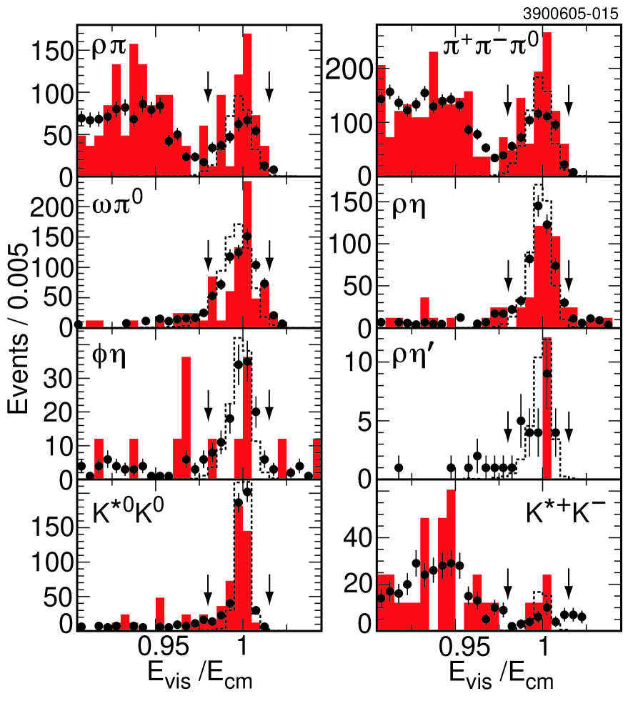
Figure 1: Scaled visible energy $E_{\mathrm{vis}}/{\sqrt{s}}$ for selected final states. Circles: data at $\sqrt{s}=3.773\,\mbox{GeV}$, shaded histogram: data at $\sqrt{s}=3.671\,\mbox{GeV}$ scaled by luminosity, dashed histogram: signal MC, arbitrary normalization. Arrows indicate selection intervals.

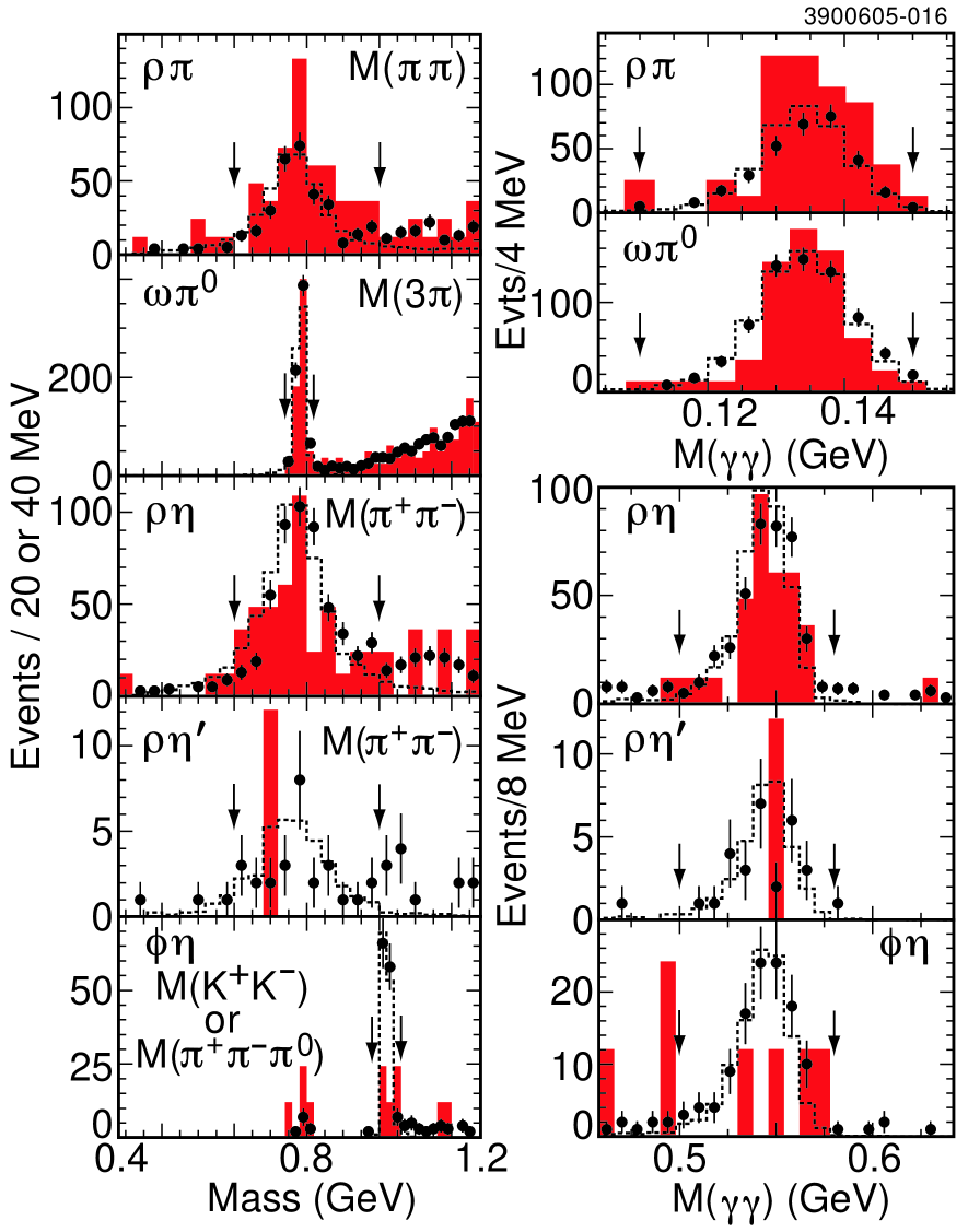
Figure 2: Reconstructed invariant mass distributions for selected final states. Symbols as in Fig. 1. The figures on the left (right) side pertain to the first (second) of the two final state particles.

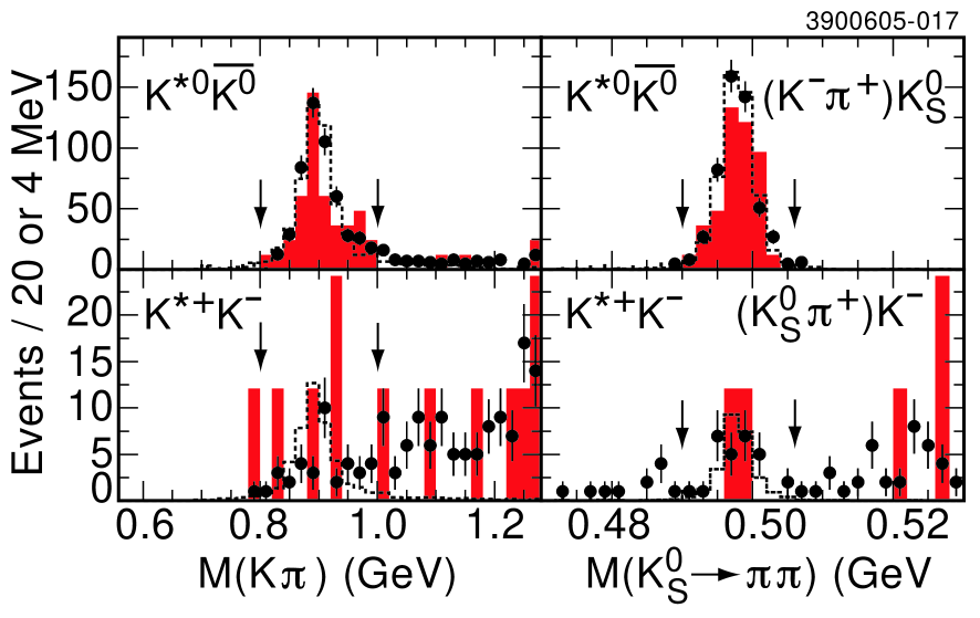
Figure 3: Mass distributions for selected final states, continued. Symbols as in Fig. 1.

We present distributions of scaled total energy $E_{\mathrm{vis}}/{\sqrt{s}}$ and reconstructed invariant masses for selected modes in Figures 1-3. All cuts other than that imposed on the quantity displayed have been applied.

The efficiency $\epsilon$ for each final state is obtained from signal Monte Carlo with the EvtGen event generator EvtGen , including final state radiation PHOTOS , and a GEANT-based detector simulation GEANT . We generated the VP modes with angular distribution $(1+\cos^{2}\theta)$ BRODLEP , $b_{1}\pi$ flat in $\cos\theta$, and $\pi^{+}\pi^{-}\pi^{0}$ as in $\omega$ decay. We assume ${\cal B}(b_{1}\to\omega\pi)$=100%.

Systematic uncertainties on the cross section measurements arise from various sources, some common to all channels, some channel specific: The systematic errors on branching fraction ratios share common contributions from the uncertainty in luminosity (1%), trigger efficiency (1%), and electron veto (0.5%). Other sources vary by channel, including cross-feed adjustments (50% of each subtraction), MC statistics, accuracy of MC-generated polar angle and mass distributions (5% for $b_{1}\pi$, 14% for $\pi^{+}\pi^{-}\pi^{0}$), and detector performance modeling quality: charged particle tracking (1%/track), $\pi^{0}$/$\eta$ and $K_{S}$ finding (2%/($\pi^{0}$/$\eta$), 5%/$K_{S}$), $\pi/K$ identification (3%/identified $\pi/K$), and resolutions of mass (2%) and total energy (1%).

Systematic uncertainties dominate in the cross section measurements for most channels at $\sqrt{s}=3.773\,\mbox{GeV}$ data and are comparable to the statistical errors for some modes at $\sqrt{s}=3.671\,\mbox{GeV}$.

The signal yields at both center-of-mass energies are listed in Table 1, separated into signal mass windows and sideband counts. Also listed are the efficiencies and cross sections. The statistical errors arise from 68% CL intervals. All cross sections include an upward correction of $(20\pm 7)$% to account for initial and final state radiation effects cleovp . In case of the isospin-violating modes, we also correct for electromagnetic interference between the tails of the $J/\psi$, $\psi(2S)$, and $\psi(3770)$ resonances with continuum production by a 4.9% upward [1.2% downward] adjustment to the cross-sections at $\sqrt{s}=3.671\,\mbox{GeV}$ [$\sqrt{s}=3.773\,\mbox{GeV}$] interferencecorrection . The results in Table 1 for $\sqrt{s}=3.671\,\mbox{GeV}$ supersede those in cleovp .

We now focus on the discrepancy between the $\sqrt{s}=3.773\,\mbox{GeV}$ yield and expected continuum contribution in order to determine whether there is significant production from $\psi(3770)$ decays. To arrive at an estimate for the continuum background at $\sqrt{s}=3.773\,\mbox{GeV}$, two routes are pursued: Method I. We scale the measured yield (after sideband subtraction) at $\sqrt{s}=3.671\,\mbox{GeV}$ by the luminosity ratio, the ratio of efficiencies ($0.88-1.00$), and an assumed dependence of $1/s^{3}$ of the continuum cross section, corresponding to a form factor dependence of $1/s$. This method uses data as much as possible, but suffers from the limiting event yield in the lower energy data sample. Using a different power $1/s^{n}$ results in a relative change of 5.4% in the scale factor per unit of $n$. Method II: We use a SU(3)-based scaling prediction, whereby the the cross sections $\sigma(e^{+}e^{-}\to\mathrm{VP})$ are linked RATIOS as $\omega\pi:\rho\eta:K^{*0}\bar{K^{0}}:\rho\pi:\rho\eta^{\prime}:\phi\eta:K^{*+}K^{-}:\phi\eta^{\prime}:\omega\eta:\omega\eta^{\prime}:\phi\pi=1:2/3:4/9:1/3:1/3:4/27:1/9:2/27:2/27:1/27:0$. By combining our data of the two isospin violating modes with highest statistics, $\omega\pi^{0}$ and $\rho\eta$ (scaled up by a factor of 3/2), we determine a unit of cross section as $\sigma^{SU(3)}=(15.1\pm 0.5)\,\mbox{pb}$ at $\sqrt{s}=3.773\,\mbox{GeV}$. This results in a precise prediction for each channel, albeit a model-dependent one. We note satisfactory agreement between the yields expected on this basis and those observed in the data at $\sqrt{s}=3.671\,\mbox{GeV}$ for all channels except of ${K^{*}}K$ (also see cleovp ). No such prediction is made for $\pi^{+}\pi^{-}\pi^{0}$ and $b_{1}\pi$.

For each channel, both continuum predictions are compared with the yield at $\sqrt{s}=3.773\,\mbox{GeV}$ by a method similar to that proposed in FELDCOUS . It is the same procedure that was applied to $\psi(2S)$ decays in cleovp : The probability that the the continuum production from either method together with the misreconstruction background as estimated from the sidebands fluctuate to an event count equal to or beyond the observed signal yield at $\sqrt{s}=3.773\,\mbox{GeV}$ is calculated with simulated trials governed by Poisson statistics. These, expressed in units of standard deviations, are included as $S^{\mathrm{I}}$ and $S^{\mathrm{II}}$ in Table 1. We find statistical agreement between the yields, with a few exceptions. The mode $\phi\eta$ is found to be enhanced over the prediction from either method: The weighted mean excess over continuum production is $(61.6\pm 11.7)$ events. This corresponds to a cross section of $\sigma^{\psi(3770)}_{\phi\eta}=(2.4\pm 0.5\pm 0.3)\,\mbox{pb}$, or, using $\sigma^{\mathrm{obs}}(\psi(3770)\to D\bar{D})=(6.39\pm 0.20)\,\mbox{nb}$ sigmaddbarcleo and removing the radiative correction factor in $\sigma^{\psi(3770)}_{\phi\eta}$, a branching fraction ${\cal B}(\psi(3770)\to\phi\eta)=(3.1\pm 0.6\pm 0.3\pm 0.1)\times 10^{-4}$, where the first error is statistical, the second systematic arising from this measurement, and the third that induced by $\sigma^{\psi(3770)}_{D\bar{D}}$. A partial width of $\Gamma_{\phi\eta}^{\psi(3770)}=(7.4\pm 1.6)\,\mbox{keV}$ follows pdg2004 . Suggestive suppressions are observed for $\pi^{+}\pi^{-}\pi^{0}$and $\rho^{0}\pi^{0}$. The observed ${K^{*}}^{0}\overline{K^{0}}$ cross section at $\sqrt{s}=3.773\,\mbox{GeV}$ is consistent with being saturated by the expected continuum production as extrapolated from $\sqrt{s}=3.671\,\mbox{GeV}$ (Method I). As the observed ${K^{*}}^{0}\overline{K^{0}}$ cross sections at both energies cleovp far exceed the SU(3) predictions (Method II), and by similar amounts, there is no indication of a substantial $\psi(3770)\to$${K^{*}}^{0}\overline{K^{0}}$ contribution. Rather, the excesses originate in the continuum process, $e^{+}e^{-}\to$${K^{*}}^{0}\overline{K^{0}}$. The same comments apply to ${K^{*}}^{+}K^{-}$, but with respect to an observed deficit obtained with Method II.

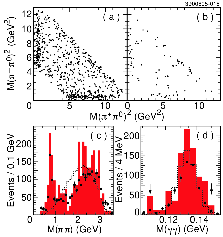
Figure 4: Dipion invariant mass distributions for the $\pi^{+}\pi^{-}\pi^{0}$ final state in data (a) at $\sqrt{s}=3.773\,\mbox{GeV}$, (b) at $\sqrt{s}=3.671\,\mbox{GeV}$. (c) The invariant mass of all pion pairs per event and (d) the reconstructed $\pi^{0}$ mass, in data at $\sqrt{s}=3.773\,\mbox{GeV}$ (circles), data at $\sqrt{s}=3.671\,\mbox{GeV}$, scaled by luminosity (shaded histogram), and phase space MC (dashed line).

Additional information on $\pi^{+}\pi^{-}\pi^{0}$ is shown in Figure 4. The dipion invariant masses in $\sqrt{s}=3.773\,\mbox{GeV}$ data shows features similar to that of $\sqrt{s}=3.671\,\mbox{GeV}$ (i.e., population of the $\rho$ mass bands together with an accumulation at higher masses); the yield reduction appears uniform in the dipion invariant mass distribution.

We compute upper limits on the event yields originating from $\psi(3770)$ decays for all modes, where we treat those with a deficit as zero counts, neglecting interference effects, and arrive at upper limits on the observable cross section excess over continuum as included in Table 1.

The measured cross sections for $\omega\pi^{0}$, $\rho\eta$, and $\rho\eta^{\prime}$ are converted into form factor measurements, which are listed in Table 2. Our results are in agreement with, but more precise than, those recently reported by BES besiv .

In summary, we have sought twelve vector pseudoscalar final states in data at $\sqrt{s}=3.773\,\mbox{GeV}$. Combined with data collected at $\sqrt{s}=3.671\,\mbox{GeV}$, we establish cross section measurements for these channels at both energies. We find evidence for the decay $\psi(3770)\to\phi\eta$, and see hints that $\psi(3770)$ decays to $\rho\pi$ and $\pi^{+}\pi^{-}\pi^{0}$ could be causing a deficit to appear in their yields through negative interference with continuum production mixing ; wmyrhopi . Otherwise, we note broad agreement with the continuum predictions. Form factor measurements for $\omega\pi^{0}$, $\rho\eta$, and $\rho\eta^{\prime}$ have been presented. All our measurements are either firsts of their kind or constitute an improvement over previous measurements.

Table 1: The number of events $N$ in the mass signal windows (“sw”) and sidebands (“sb”) in data taken at $\sqrt{s}=3.671\,\mbox{GeV}$ and $\sqrt{s}=3.773\,\mbox{GeV}$ data; the efficiency $\epsilon$ in percent; the level of consistency or significance, expressed in units of standard deviations, between continuum background and observed yield, for the two methods of determining the continuum background described in the text, $S^{\mathrm{I}}$ and $S^{\mathrm{II}}$; the cross sections at $\sqrt{s}=3.671\,\mbox{GeV}$ and $\sqrt{s}=3.773\,\mbox{GeV}$; the cross section $\psi(3770)\to h_{1}h_{2}$, computed as the excess over the continuum prediction as established using Method I or Method II (see text).

Channel	$N^{3.67}_{\mathrm{sw}}$	$N^{3.67}_{\mathrm{sb}}$	$N^{3.77}_{\mathrm{sw}}$	$N^{3.77}_{\mathrm{sb}}$	$\epsilon$	$S^{\mathrm{I}}$	$S^{\mathrm{II}}$	$\sigma^{\mathrm{3.67GeV}}\ [\,\mbox{pb}]$	$\sigma^{\mathrm{3.77GeV}}\ [\,\mbox{pb}]$	$\sigma_{\psi(3770)}^{\mathrm{I}}\ [\,\mbox{pb}]$	$\sigma_{\psi(3770)}^{\mathrm{II}}\ [\,\mbox{pb}]$
$\pi^{+}\pi^{-}\pi^{0}$	74	6.8	576	72.3	29.0	-2.7		$13.1^{+1.9}_{-1.7}\pm 2.1$	$7.4\pm 0.4\pm 1.2$	$<$ 0.04
$\rho\pi$	43	5.4	314	44.8	26.3	-2.2	-1.7	$8.0^{+1.7}_{-1.4}\pm 0.9$	$4.4\pm 0.3\pm 0.5$	$<$ 0.04	$<$ 0.04
$\rho^{0}\pi^{0}$	21	3.4	130	33.0	32.5	-2.2	-2.1	$3.1^{+1.0}_{-0.8}\pm 0.4$	$1.3\pm 0.2\pm 0.2$	$<$ 0.03	$<$ 0.03
$\rho^{+}\pi^{-}$	22	2.0	184	11.8	23.1	-0.9	-0.5	$4.8^{+1.5}_{-1.2}\pm 0.5$	$3.2\pm 0.3\pm 0.3$	$<$ 0.05	$<$ 0.05
$\omega\pi^{0}$	54	6.2	696	39.2	19.0	0.9	-0.2	$15.2^{+2.8}_{-2.4}\pm 1.5$	$14.6\pm 0.6\pm 1.5$	$<$ 4.5	$<$ 0.06
$\phi\pi^{0}$	1	1.6	2	4.0	16.5	0.0	-0.0	$<2.2$	$<0.2$	$<$ 0.2	$<$ 0.2
$\rho\eta$	36	3.1	508	31.0	19.6	1.1	0.7	$10.0^{+2.2}_{-1.9}\pm 1.0$	$10.3\pm 0.5\pm 1.0$	$<$ 4.0	$<$ 1.3
$\omega\eta$	4	0.0	15	6.0	9.9	-1.7	-2.9	$2.3^{+1.8}_{-1.0}\pm 0.5$	$0.4\pm 0.2\pm 0.1$	$<$ 0.1	$<$ 0.1
$\phi\eta$	5	1.0	132	15.9	11.0	2.5	$\geq 5$	$2.1^{+1.9}_{-1.2}\pm 0.2$	$4.5\pm 0.5\pm 0.5$	$<$ 4.5	$<$ 3.3
$\rho\eta^{\prime}$	1	0.0	27	0.9	2.9	1.0	-1.3	$2.1^{+4.7}_{-1.6}\pm 0.2$	$3.8^{+0.9}_{-0.8}\pm 0.4$	$<$ 4.7	$<$ 0.4
$\omega\eta^{\prime}$	0	0.0	2	0.0	1.5	$\geq 5$	0.0	$<17.1$	$0.6^{+0.8}_{-0.3}\pm 0.6$	$<$ 3.0	$<$ 1.9
$\phi\eta^{\prime}$	0	0.0	9	2.0	1.2	2.4	1.2	$<12.6$	$2.5^{+1.5}_{-1.1}\pm 0.4$	$<$ 5.2	$<$ 3.8
${K^{*}}^{0}\overline{K^{0}}$	38	0.4	501	18.1	8.8	1.1	$\geq 5$	$23.5^{+4.6}_{-3.9}\pm 3.1$	$23.5\pm 1.1\pm 3.1$	$<$ 9.0	$<$ 20.8
${K^{*}}^{+}K^{-}$	4	1.0	36	32.4	16.0	-1.4	-4.1	$1.0^{+1.1}_{-0.7}\pm 0.5$	$<0.6$	$<$ 0.1	$<$ 0.1
$b_{1}\pi$	20	4.5	268	100.3	11.3	-0.1		$7.9^{+3.1}_{-2.5}\pm 1.8$	$6.3\pm 0.7\pm 1.5$	$<$ 0.1
$b_{1}^{0}\pi^{0}$	5	3.0	49	82.5	4.2	-1.2		$<17.1$	$<2.5$	$<$ 0.4
$b_{1}^{+}\pi^{-}$	15	1.5	219	17.8	18.4	1.0		$4.2^{+1.6}_{-1.2}\pm 0.6$	$4.7\pm 0.4\pm 0.6$	$<$ 2.7

Table 2: Form factors with statistical and systematic errors.

Channel	${\cal F}(s)\ (\mbox{TeV}^{-1})$
	$\sqrt{s}=3.671\,\mbox{GeV}$	$\sqrt{s}=3.773\,\mbox{GeV}$
$\omega\pi^{0}$	$40^{+4}_{-3}\pm 2$	$39\pm 1\pm 2$
$\rho\eta$	$34^{+4}_{-3}\pm 2$	$34\pm 1\pm 2$
$\rho\eta^{\prime}$	$17^{+14}_{-9}\pm 1$	$22^{+3}_{-2}\pm 1$

References

(1) J.L. Rosner, Phys. Rev. D 64, 094002 (2001).
(2) BES Collaboration, J.Z. Bai et al.,
Phys. Lett. B 605, 63 (2005);
CLEO Collaboration, N.E. Adam et al.,
hep-ex/0508023 (subm. to Phys. Rev. Lett.);
CLEO Collaboration, G.S. Huang et al.,
hep-ex/0509046 [Phys. Rev. Lett (to be published)];
CLEO Collaboration, T.E. Coan et al.,
hep-ex/0509030 (subm. to Phys. Rev. Lett.);
CLEO Collaboration, D. Besson et al.,
hep-ex/0512038 (subm. to Phys. Rev. Lett.).
(3) CLEO Collaboration, N.E. Adam et al.,
Phys. Rev. Lett. 94, 012005 (2005).
(4)