Precise Measurement of Neutrino and Anti-neutrino Differential Cross Sections

Abstract

The NuTeV experiment at Fermilab has obtained a unique high statistics sample of neutrino and anti-neutrino interactions using its high-energy sign-selected beam. We present a measurement of the differential cross section for charged-current neutrino and anti-neutrino scattering from iron. Structure functions, $F_{2}(x,Q^{2})$ and $xF_{3}(x,Q^{2})$, are determined by fitting the inelasticity, $y$, dependence of the cross sections. This measurement has significantly improved systematic precision as a consequence of more precise understanding of hadron and muon energy scales.

I Introduction

Deep inelastic scattering (DIS), the scattering of a high energy lepton off a quark inside a nucleon, has been a proving ground for QCD, the theory of strong interactions. Charged-leptons and neutrinos have been used to measure parton densities and their QCD evolution with high-precision over a wide range in $Q^{2}$. Uniquely, neutrino DIS, via the weak interaction probe, allows simultaneous measurement of two structure functions: $F_{2}(x,Q^{2})$ and the parity-violating structure function, $xF_{3}(x,Q^{2})$.

In this paper we present a new measurement of high-energy neutrino and anti-neutrino differential cross sections from high-statistics data samples. The differential dependence of neutrino and anti-neutrino cross sections on Bjorken scaling variable, $x$, and inelasticity, $y$, provide the most model-independent physics observable for this process [1]. Previous high-statistics measurements of the neutrino and anti-neutrino differential cross section have been reported [2], [3]. This experiment has two improvements: first, a sign-selected beam allowed separate neutrino and antineutrino running and, second, a calibration beam continuously measured the detector’s response. The largest experimental uncertainties in previous measurements arose from knowledge of energy scale and detector response functions [4], [5]. NuTeV addressed this by using a dedicated calibration beam of hadrons, electrons and muons that alternated with neutrino running once every minute throughout the one year data-taking peroid. The calibration beam was used to measure the detector response for hadrons and muons over a wide range of energies (5-200 GeV). Detector response functions and energy scales for muons and hadrons were mapped over the full active area of the detector. Energy scales for muons and hadrons were determined to a precision of 0.43% for hadrons and 0.7% for muons [6]. NuTeV’s other improvement was separate neutrino and antineutrino running. NuTeV ran in two modes, ($\nu$ and $\overline{\nu}$), with the muon spectrometer polarity always set to focus the primary charged-lepton from the interaction vertex (e.g. $\mu^{-}$ in $\nu$-mode or $\mu^{+}$ in $\overline{\nu}$-mode). In determining the charged-current differential cross sections, this allowed better and more uniform acceptance in the two running modes and removed ambiguity in the muon sign determination present in a mixed $\nu$ and $\overline{\nu}$ beam.

The rest of this paper is organized into four parts; Section II describes the NuTeV detector, Section III gives the cross section extraction method and results, and Section IV presents the extracted structure functions and the results are discussed in Section V.

II NuTeV Experiment

The NuTeV experiment collected data during 1996-97 using separate high-purity $\nu_{\mu}$ and $\overline{\nu}_{\mu}$ beam produced by the Sign-Selected Quadrupole Train (SSQT) beamline. A dipole magnet after the one-interaction-length beryllium oxide production target allowed the sign of secondary particles to be selected. Neutrinos (or anti-neutrinos) are produced when sign-selected secondary pions and kaons decay in the $440$ m decay region located just downstream of SSQT optics. The NuTeV neutrino detector is $1.4$ km downstream of the beryllium oxide production target. Neutrino energies ranged from 30-500 GeV. Figure 1 shows a prediction of the interacting $\nu_{\mu}$ and $\overline{\nu}_{\mu}$ flux in each mode with it’s small contribution from the wrong-sign background. The interacted neutrino fraction from $\overline{\nu}$($\nu$) in $\nu$($\overline{\nu}$)-mode is $3\times 10^{-4}$ ($4\times 10^{-3}$).

FIG. 1.: Predicted energy spectrum of interacted muon-neutrinos anti-neutrinos when the SSQT is set to select neutrinos (top) and antineutrinos (bottom).

The NuTeV/CCFR detector consisted of an 18 m long, 690 ton target calorimeter with a mean density of ${\rm 4.2~{}g/cm^{3}}$, followed by a 420 ton iron toroidal spectrometer. The target was composed of 168 steel plates, each ${\rm 3m\times 3m\times 5.15cm}$, instrumented with liquid scintillator counters placed every two steel plates and drift chambers spaced every four plates. NuTeV refurbished the CCFR detector by replacing the scintillator oil and reconditioning the drift chambers.

Immediately downstream of the target-calorimeter was a magnetized iron toroidal spectrometer with inner radius 12.5 cm and outer radius 175 cm used to measure the momentum of high-energy muons exiting the downstream end of the target. The toroid spectrometer consisted of three magnetized sections each followed by a drift chamber station. Two additional drift chamber stations were located a few meters downstream of the last magnetic section to analyze the highest momentum muons. The magnetic field in each toroidal section ($\sim$15 kG) was produced by four copper coils which emerged through the center hole. The magnetic field is azimuthal everywhere except for a small radial component in the region of the supporting feet and air gap between top and bottom halves of the washers. The azimuthal component of the field in the first toroid had an additional small asymmetry (with respect to vertical) due to a shorted coil on the west side. The detailed geometry of the spectrometer, (including the missing coil), was input to ANSYS simulation [7] to compute the magnetic field map.

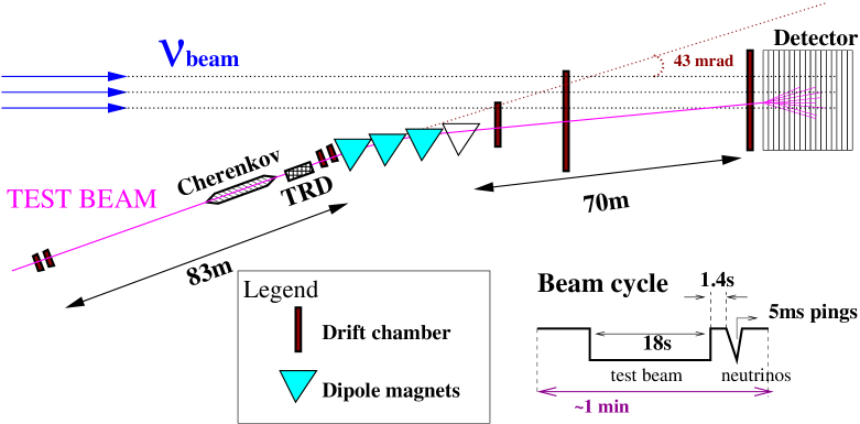
FIG. 2.: Sketch of calibration beam spectrometer configuration. The calibration beam ran alternating with neutrinos once a minute for the entire NuTeV data-taking period.

A dedicated in situ calibration beam was used to determine the energy response of the calorimeter and spectrometer to hadrons, muons, and electrons and to map the response over the face of the detector. The tolerance of the calibration spectrometer to measure a beam particle’s absolute momentum was 0.3%. The configuration is shown in Figure 2. Details of the calibration and response measurements are given in [6]. The hadronic resolution of the calorimeter was determined to be $\frac{\sigma}{E}=\frac{86\%}{\sqrt{E}}\oplus 2.2\%$ with an absolute scale uncertainty of $\frac{\delta E}{E}=0.43\%$. The latter uncertainty is dominated by the statistical precision in calibrating the time dependence of the counter response over a transverse grid for each counter.

The absolute scale of the toroid spectrometer was calibrated with muons that were steered over the active area of the spectrometer. The magnetic field map from the ANSYS simulation was checked with the 50 GeV muon calibration beam. The mean reconstructed muon momentum compared with the muon calibration beam had a 1$\sigma$ variation of 0.63% over the active area of the toroid. This field map uncertainty is attributed to variation in magnetic susceptibility and thickness of the steel. The field map determination dominates the absolute muon energy scale uncertainty of 0.7%.

III Cross Section Measurement

In charged-current (CC) neutrino DIS the $\nu$ scatters off a quark in the nucleon via exchange of a virtual $W$-boson. The cross section can be expressed in terms of structure functions, $2xF_{1}(x,Q^{2})$, $F_{2}(x,Q^{2})$, and $xF_{3}(x,Q^{2})$

$$\frac{d^{2}\sigma^{\nu(\overline{\nu})}}{dxdy} = \frac{G_{F}^{2}ME}{\pi}{\Big{(}}\Big{[}1-y(1+\frac{Mx}{2E})+\frac{y^{2}}{2}\frac{1+(\frac{2Mx}{Q})^{2}}{1+R_{L}}\Big{]}$$ (2)

$$F_{2}(x,Q^{2})\pm\Big{[}y-\frac{y^{2}}{2}\Big{]}xF_{3}(x,Q^{2}){\Big{)}}$$

where $G_{F}$ is the Fermi weak coupling constant, $M$ is the proton mass, $E_{\nu}$ is the incident neutrino energy in the lab frame, and $y$, the inelasticity, is the fraction of energy transferred to the hadronic system. The $xF_{3}$ term is added for neutrino interactions and is subtracted for antineutrinos. $R_{L}(x,Q^{2})$, the ratio of the cross section for scattering from longitudinally to transversely polarized W-bosons relates $F_{2}(x,Q^{2})$ and $2xF_{1}(x,Q^{2})$

$$2xF_{1}=F_{2}\Big{(}\frac{1+{(\frac{2Mx}{Q})^{2}}}{1+R_{L}(x,Q^{2})}\Big{)}.$$

Structure functions depend on $x$, the Bjorken scaling variable, and $Q^{2}$, the four momentum squared of the virtual W-boson.

Relativistic invariant kinematic variables, $x$, $y$, and $Q^{2}$ can be evaluated in the lab frame using the three experimentally measured quantities: $E_{\mu}$, energy of the outgoing primary charged-lepton, $E_{\rm\scriptstyle HAD}$ the energy deposited at the hadronic vertex, and $\theta_{\mu}$, the scattering angle of the primary muon.

$$x=\frac{4E_{\nu}E_{\mu}sin^{2}\frac{\theta_{\mu}}{2}}{2ME_{\rm\scriptstyle HAD}},$$

$$y=E_{\rm\scriptstyle HAD}/E_{\nu},~{}~{}\rm{and}$$

$$Q^{2}=2MxyE_{\nu}$$

where the neutrino energy, $E_{\nu}=E_{\mu}+E_{\rm\scriptstyle HAD}$, is reconstructed from the measured final state particle energies.

A Event Reconstruction

Events used in this analysis were triggered by the presence of a penetrating muon track determined by in-time hits in scintillation counters in the most downstream region of the target calorimeter and in the first station of the toroid spectrometer. This allowed acceptance for charged current events down to zero hadron energy.

$E_{\rm\scriptstyle HAD}$ is determined by summing the pulse heights of consecutive counters from just downstream of the event vertex to five counters beyond the end of the shower region. Longitudinal position of the event vertex is defined as the first of at least two consecutive counters with greater than four times the energy deposited by a minimum ionizing particle (MIP). The end of the shower region is the last counter before three consecutive counters with less than four MIP’s. Energy deposited by the primary muon in this region is removed by subtracting the most probable energy loss for each counter in the sum. This energy is included in the reconstructed muon energy.

$E_{\mu}$ at the event vertex is reconstructed in two parts: energy deposited in the target calorimeter (typically less than 10 GeV) and remaining energy that is measured in the downstream toroid spectrometer. Energy deposited in the target calorimeter includes the muon energy within the shower region (discussed above) and energy deposited beyond the shower region before the muon exits the calorimeter. The latter is determined from the pulse height of energy deposited in each counter by the muon. For small pulse heights, ($<5$ MIPs), the muon energy loss is assumed to arise from ionization processes and is converted to GeV using an $E_{\mu}$ dependent conversion function which was optimized using GEANT to reproduce both the most probable value and the width of this component of the energy loss (see [6]). For larger pulse heights ($>5$ MIPs), the energy is assumed to have a contribution from catastrophic processes (i.e. bremsstrahlung, pair production). Therefore, the additional amount above 5 MIPs is converted to GeV using a calibration constant determined from the calorimeter’s electromagnetic response. The contribution to the muon energy resolution from determination of energy loss in the target is small for high energy muons and dominated by a long tail produced by catastrophic energy loss processes.

Muons that enter the toroid spectrometer are focused and tracked through the spectrometer where they are momentum analyzed. Figure 3 shows the momentum resolution for the toroid spectrometer determined using test beam muons. The Gaussian contribution is dominated by multiple Coulomb scattering (MCS) and is independent of momentum ($\sim$ 11%). The high-end tail is due to catastrophic energy loss processes. Test beam data are used to parameterize the resolution functions using a fit of the form

$$\frac{\Delta\left(1/P_{\mu}\right)}{\left(1/P_{\mu}\right)} = exp\left[-\frac{1}{2}\frac{x^{2}}{\sigma^{2}_{lead}(P_{\mu})}\right]$$ (3)

$$+ R_{tail}(P_{\mu})exp\left[-\frac{1}{2}\frac{(x-x_{tail}(P_{\mu}))^{2}}{\sigma^{2}_{tail}(P_{\mu})}\right],$$ (4)

where $\sigma_{lead}(P_{\mu})$ is the width of the leading Gaussian contribution due to MCS, and $R_{tail}(P_{\mu})$, $\sigma_{tail}(P_{\mu})$ and $x_{tail}(P_{\mu})$ are the normalization coefficient, the width and the offset of the asymmetric tail of the resolution function. These parameters are found to have small energy dependences. The width of the leading Gaussian is parameterized with the following function

$$\sigma_{lead}(P_{\mu})=\sqrt{A^{2}+(BP_{\mu})^{2}},$$ (5)

where $A=0.10$ and $B=4.2\times 10^{-3}$. $R_{tail}(P_{\mu})$, $\sigma_{tail}(P_{\mu})$, and $x_{tail}(P_{\mu})$ are parameterized with linear functions. For a muon entering the toroid with momentum $P_{\mu}=$100 GeV the resolution function parameters have the following values $\sigma_{lead}(100)=0.11$, $\sigma_{tail}(100)=0.47$, $x_{tail}(100)=0.18$, and $R_{tail}(100)=0.079$.

FIG. 3.: Test beam data (points) with muon momentum of 100 GeV measured in the toroid spectrometer compared with double Gaussian fit parameterization curve.

Muon angle is determined using the track vector in the target calorimeter extrapolated back to the event vertex. Resolution on muon angle is dominated by multiple scattering in the target and is determined from GEANT hit-level simulation of the detector. Angular resolution (in $mRad$) is parameterized as

$$\Delta\theta_{\mu}=(96.8+0.87~{}L+0.24~{}E_{\rm\scriptstyle HAD})/P_{\mu}$$

for a muon with momentum ${P_{\mu}}$ (in GeV) where $L$ is the track length in the target in units of counters, and $E_{\rm\scriptstyle HAD}$ is the shower energy in GeV. The small dependence on hadron energy comes from an $E_{\rm\scriptstyle HAD}$ dependent cut excluding tracking chambers near the event vertex due to the presence of additional hits in the shower region.

B Data Selection

The following criteria were used to select the events for the cross section sample:

• Event containment: transverse vertex within 125 cm from detector center and longitudinal vertex at least four counters beyond the upstream end of the detector and beginning at least twenty counters from the downstream end.

• Reconstructed muon energy: A single muon in the event with minimum energy, $E_{\mu}>15$ GeV.

• Reconstructed muon track in toroid: transverse position within, $15<$ radius $<160$ cm upon entering; minimum penetration of track to the second chamber station; and minimum fraction of integrated track in steel $\geq 80\%$.

• Reconstructed hadronic energy: $E_{HAD}>10$ GeV.

• Reconstructed neutrino energy: $30<E_{\nu}<360$ GeV, is required to ensure that the flux is well understood and the muon momentum well reconstructed.

• Reconstructed $Q^{2}$: $Q^{2}>1$ GeV², is required to ensure that non-perturbative contributions in our cross section model are small.

• Reconstructed Bjorken-$x$: $x<0.8$. Data at higher $x$ are excluded because smearing effects are large and our model is not well constrained in this region.

The final samples passing these cuts contained $8.6\times 10^{5}$ neutrino ($\nu_{\mu}$) and $2.4\times 10^{5}$ anti-neutrino ($\overline{\nu}_{\mu}$) events.

The differential cross section is determined from the differential number of events and the flux, $\Phi(E)$, at a given neutrino energy,

$$\frac{d^{2}\sigma^{\nu(\overline{\nu})}_{ijk}}{dxdy}\propto\frac{1}{\Phi(E_{i})}\frac{\Delta N^{\nu(\overline{\nu})}_{ijk}}{\Delta x_{j}\Delta y_{k}}.$$ (6)

The quantity $\frac{d^{2}\sigma^{\nu(\overline{\nu})}_{ijk}}{dxdy}$ represents the average differential cross section in bin $ijk$. The absolute flux was not measured in NuTeV. The flux was normalized so that the average NuTeV total cross section from 30-200 GeV is equal to the world average value (see section III C).

The number of events in a given bin, $N^{\nu(\overline{\nu})}_{ijk}$, must be corrected for bin acceptance due to detector geometry and kinematic cuts, and for bin migration caused by experimental resolution. The cross section measured in Equation 6 is corrected to the bin-center value

$$\frac{d^{2}\sigma^{\nu(\overline{\nu})}}{dxdy}(E^{c}_{i},x^{c}_{j},y^{c}_{k})=\frac{d^{2}\sigma^{\nu(\overline{\nu})}_{ijk}}{dxdy}\times\frac{S(E^{c}_{i},x^{c}_{j},y^{c}_{k})}{\overline{S}_{ijk}}$$ (7)

where $S(E^{c}_{i},x^{c}_{j},y^{c}_{k})$ is the differential cross section evaluated at the bin-center values $E^{c}_{i},x^{c}_{j},y^{c}_{k}$ and $\overline{S}_{ijk}$ is the average value of the cross section determined from the integral over the bin

$$\overline{S}_{ijk}=\frac{1}{\Delta x_{j}\Delta y_{k}}\int^{x_{j}+1}_{x_{j}}\int^{y_{k}+1}_{y_{k}}\frac{d^{2}\sigma(E_{i},x,y)}{dxdy}~{}dx~{}dy.$$

This correction is calculated by integration of the Monte Carlo model (described in section III D) and is most important at low and high $x$.

C Neutrino Flux

The neutrino (and antineutrino) relative flux as a function of energy is determined using the “fixed $\nu_{o}$” method [4]. Integrating the differential cross section given in eq. 2 over $x$ gives

$${\frac{d\sigma}{d\nu}}=A\left(1+\frac{B}{A}\frac{\nu}{E}-\frac{C}{A}\frac{\nu^{2}}{2E^{2}}\right)$$ (8)

where $\nu=E_{\rm\scriptstyle HAD}$ and $E$ is the incident neutrino energy. The coefficients are given by,

$$A=\frac{G_{F}M}{\pi}\displaystyle\int F_{2}(x)dx$$

$$B=-\frac{G_{F}M}{\pi}\displaystyle\int\Big{(}F_{2}(x)\mp xF_{3}(x)\Big{)}dx$$

$$C = B-\frac{G_{F}M}{\pi}\displaystyle\int F_{2}(x)R_{\rm\scriptstyle TERM}dx$$ (9)

where, $R_{\rm\scriptstyle TERM}=\left(\frac{1+\frac{2Mx}{\nu}}{1+R_{L}}-\frac{Mx}{\nu}-1\right)$, depends on the longitudinal structure function, $R_{L}(x)$. Multiplying both sides of eq. 8 by the flux $\Phi(E)$ gives the number of events

$${\frac{dN}{d\nu}}=\Phi(E)A\left(1+\frac{B}{A}\frac{\nu}{E}-\frac{C}{A}\frac{\nu^{2}}{2E^{2}}\right).$$

As $\nu\rightarrow 0$ the cross section (eq. 8) is independent of energy and therefore the number of events at low $\nu$ is proportional to the flux, $\frac{dN}{d\nu}\rightarrow\Phi(E)A$. To minimize the statistical uncertainty, data up to $\nu=20GeV$ are included in our flux sample. Therefore a correction is applied to account for the energy dependence as discussed below. Substituting for the coefficient C, the relative flux is then given by

$$\Phi({\rm E})=\displaystyle\int_{0}^{\nu_{0}}\frac{\frac{dN({\rm\scriptstyle E})}{d\nu}}{1+\langle\frac{B}{A}\rangle\left(\frac{\nu}{E}-\frac{\nu^{2}}{2E^{2}}\right)+\frac{\nu^{2}}{2E^{2}}\frac{\int F_{2}(x)R_{\rm\scriptscriptstyle{TERM}}}{\int F_{2}(x)}}\,d\nu.$$

The term $\int F_{2}(x)R_{\rm\scriptscriptstyle{TERM}}/\int F_{2}(x)$ is obtained by integrating the structure functions, calculated using our Monte Carlo model.

In reference [4] it was assumed that the coeficients $A$ and $B$ do not depend on $\nu$. The integration over $x$ at fixed $\nu$ gives an implicit $Q^{2}$ dependence, $Q^{2}=2Mx\nu$. For different values of $\nu$ the integral will be over different ranges in $Q^{2}$. A $\nu$-dependent scaling violations correction is applied to account for this effect. The correction is obtained by integrating the structure functions $F_{2}$ and $xF_{3}$ over $x$ at fixed $\nu$, using our Monte Carlo model. As described below, this correction shifts the measured value of $\frac{B}{A}$ and has a small effect on the extracted flux.

The flux data sample consists of events which are contained in the detector, have a well constructed muon with minimum energy $E_{\mu}>15$ GeV, neutrino energy in the range $30<E<360$ GeV, and $E_{\rm\scriptstyle HAD}<20$ GeV. The $E_{\rm\scriptstyle HAD}$ cut makes this sample orthogonal to the sample used to measure the cross sections. The data are corrected for acceptance and detector effects using our Monte Carlo model. Corrections were also applied to remove QED radiative effects using [12] and for the charm production threshold using a leading-order slow rescaling model with the charm mass parameter, $m_{c}=1.40\pm 0.18$ (see Appendix). Radiative corrections range from -2% at 30 GeV to 4% at 290 GeV. The charm production correction decreases with energy and is about 5% for the flux sample at 30 GeV.

The coefficient $\frac{B}{A}$ is determined from a fit to $\frac{dN}{d\nu}$ over the range $5<\nu<20$ GeV. Limiting $\nu$ to above 5 GeV reduces the contribution from quasi-elastic and resonance processes, which are difficult to model. The coefficients of the fit parameters $A$ and $B$ are modified to remove the $\nu$ dependence due to scaling violations. The fit is performed for each energy and the average value of $\langle\frac{B}{A}\rangle$ over all energy bins is used. We obtain $\langle\frac{B}{A}\rangle=-0.34\pm 0.04$ for neutrinos and $-1.68\pm 0.03$ for anti-neutrinos. The effect of scaling violations is to shift the average value of $\langle\frac{B}{A}\rangle$ by $+$0.13 for neutrinos and $+$0.03 for anti-neutrinos. The effect on the extracted neutrino flux ranges from 3.5% at 35 GeV and is negligible above 120 GeV for neutrinos. For anti-neutrinos the correction to $\langle\frac{B}{A}\rangle$ is small and the effect on the flux is less than 0.8% for all energies. Because the scaling violations correction is calculated from a model we estimate a systematic uncertainty in $\langle\frac{B}{A}\rangle$ to be 0.05(0.04) for neutrinos(anti-neutrinos). This theoretical uncertainty is obtained by using an alternative model [13] to evaluate the scaling violations and to extract $\langle\frac{B}{A}\rangle$. The value of $\frac{B}{A}$ computed directly from the NuTeV cross section model (at $\nu=20$ Gev) gives -0.29 for neutrinos and -1.66 for antineutrinos which compares well with the value computed for the alternative cross section model (Bodek-Yang) from reference [13] which gives -0.28 and -1.68, respectively.

The total cross section is used to normalize the flux. A sample of events are selected which are contained in the detector and have well constructed muon with minimum energy $E_{\mu}>15$ GeV. The total neutrino(antineutrino) cross section is

$$\frac{\sigma^{\nu(\overline{\nu})}(E)}{E}=\frac{N^{\nu(\overline{\nu})}(E)}{E\cdot\Phi({\rm E})},$$

where $N^{\nu(\overline{\nu})}(E)$ is the number of total cross section events, corrected for acceptance and detector effects, and $\Phi({\rm E})$ is the relative flux.

The flux is normalized using the world average neutrino cross section from 30-200 GeV [8].

$$\frac{\sigma^{\nu}}{E}=0.677\pm 0.014~{}~{}\times 10^{-38}~{}\frac{\rm\scriptstyle cm^{2}}{\rm\scriptstyle GeV}$$

The cross section normalization uncertainty, 2.1%, arises from the quoted errors on the world average absolute neutrino cross section. Figure 4 shows the energy dependence of the total cross section, $\frac{\sigma}{E}$. The total neutrino and antineutrino cross sections are linear with energy to better than 2% over our energy range. The relative $\overline{\nu}$ to $\nu$ cross section, $r=\frac{\sigma^{\overline{\nu}}}{\sigma^{\nu}}$, can be measured from NuTeV data alone which gives a value of $r=0.505\pm 0.0018$(stat)$\pm 0.0029$(syst). This measurement is the most accurate determination to date and it agrees with the previous world average value of $r=0.499\pm 0.007$.

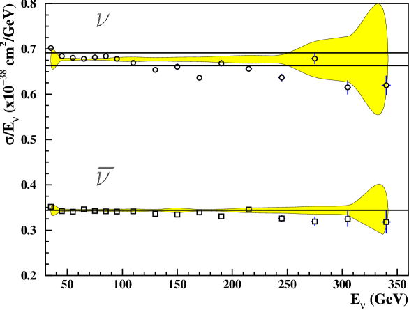
FIG. 4.: Total cross section, $\frac{\sigma}{E}$, as a function of energy for neutrino (circles) and anti-neutrino (squares) interactions. The error bars are statistical uncertainty and the yellow band shows the size of the systematic uncertainty.

D Cross Section Extraction

The Monte Carlo simulation, used to account for acceptance and resolution effects, requires an input cross section model which is iteratively tuned to fit our data. Our cross section model, described in the Appendix, is based on a leading order prescription from Buras and Gaemers[9] that is modified to incorporate higher-order corrections such as $R_{L}(x,Q^{2})$, charm mass, and higher-twist effects which are important at low $Q^{2}$. Cross section data are fit to determine empirically a set of parton distribution functions. To model regions at the edge of our data sensitivity we use additional input to constrain the cross section. At high-$x$ and low $Q^{2}$ we model higher-twist contributions following reference [10] by incorporating charged-lepton data in the fit. At low $x$ and low $Q^{2}$, (below 1.35 GeV²), where the Buras-Gaemers parameterization is not well behaved, the shape of GRV94LO [11] is used.

The cross section, flux, and the model parton distribution functions ($PDF$s) are obtained by a reiterative extraction and refitting proceedure. An initial set of model parameters from CCFR[3] are used to extract an initial flux and cross section. From these we perform a fit to obtain a set of $PDF$s which are then used to extract a new flux and cross section. The proceedure is reiterated until the relative change in cross section value from one iteration to the next averaged over all the data points is less than 0.1% (this occurs within three iterations). New radiative corrections calculated from [12] are computed for each new cross section fit. After the final iteration, we exclude kinematic bins where the number of events generated in that bin account for less than 20% of the events. This reduces the contribution from the high $E_{\mu}$ tail where smearing dominates the distribution.

Figure 5 shows a comparison of the distributions of the three kinematic variables measured in data with those determined from the Monte Carlo model. The data versus model $\chi^{2}$ including systematic uncertainties is $\chi^{2}/dof=2225/2599$. If full point-to-point data correlations are included in the $\chi^{2}$ the fit quality worsens to $\chi^{2}/dof=3534/2599$. (The data correlation matrix is discussed in Section III F). The inclusion of the extremely precise charged-lepton data in our model fit (see Appendix) has the effect of systematically pulling the $Q^{2}$ dependence of the model into agreement with the charged-lepton data and worsens the quality of the model fit with NuTeV data. Alternative models based on global parton distribution fits give a significantly poorer $\chi^{2}$ with our data; the Bodek-Yang model from reference [13] gives $\chi^{2}=5969/2599$ and TRVFS(MRST99) [14] gives $\chi^{2}=5000/2599$. Model sensitivity in the cross section measurement is small (see section III F).

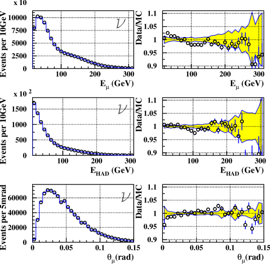
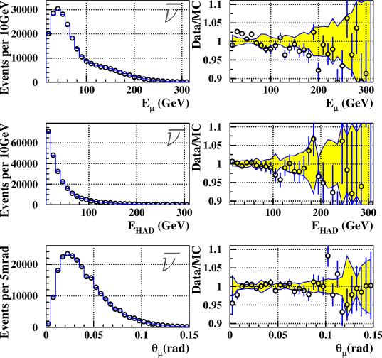
FIG. 5.: Comparison of data distributions for kinematic variables, $E_{\mu}$, $E_{HAD}$, and $\theta_{\mu}$ with Monte Carlo simulation for neutrinos (top) and anti-neutrinos (bottom). The points are data and the curve is the Monte Carlo model. Ratio of data to Monte Carlo is plotted at the right of each distribution. The error bars are statistical uncertainty and the yellow band shows the size of the systematic uncertainty.

E Results

Figures 6-8 show the extracted $\nu-Fe$ and $\overline{\nu}-Fe$ cross sections plotted as a function of $y$ for a representative sample of $x$ bins at neutrino energies of $65$ GeV, $150$ GeV, and $245$ GeV respectively. The NuTeV data are compared with measurements from CCFR [3] and at lower energies with CDHSW data [2]. The curve shown is the parameterization fit to the NuTeV data. The three data sets are in reasonable agreement in both level and shape at low and moderate $x$. There are differences in NuTeV and CCFR cross sections at $x>0.40$ where CCFR’s measurement for both $\nu$ and $\overline{\nu}$ cross sections are consistently below the NuTeV result over the entire energy range. The level difference in the cross sections for these bins at a given $x$ is constant over the full $y$ range of the data. The difference in the neutrino cross sections are $4\pm 1\%$ at $x=0.45$, $9\pm 2\%$ at $x=0.55$, and increases with $x$ up to $18\pm 2\%$ at $x=0.65$, (and similarly for antineutrinos). This discrepancy and its probable source are discussed in Section V.

FIG. 6.: Differential cross sections in $x$ bins for neutrinos (left) and anti-neutrinos (right) at $E=65$ GeV. Points are NuTeV (filled circles), CCFR (open squares), and CDHSW (crosses). Error bars show statistical and systematic errors in quadrature. Solid curve shows fit to NuTeV data. ($x=$0.08, 0.225, 0.45, and 0.75 bins are not shown).

FIG. 7.: Differential cross sections in $x$ bins for neutrinos (left) and anti-neutrinos (right) at $E=150$ GeV. Points are NuTeV (filled circles), CCFR (open squares), and CDHSW (crosses). Error bars show statistical and systematic errors in quadrature. Solid curve shows fit to NuTeV data. ($x=$0.08, 0.225, 0.45, and 0.75 bins are not shown).

FIG. 8.: Differential cross sections in $x$ bins for neutrinos (left) and anti-neutrinos (right) at $E=245$ GeV. Points are NuTeV (filled circles), CCFR (open squares), and CDHSW (crosses). Error bars show statistical and systematic errors in quadrature. Solid curve shows fit to NuTeV data. ($x=$0.08, 0.225, 0.45, and 0.75 bins are not shown).

F Systematic Uncertainties

We evaluated the contribution from seven experimental systematic uncertainties on the cross section measurement error. These include uncertainties in the following: muon and hadron energy scales, muon and hadron energy smearing, the charm mass value $m_{c}$ and $\frac{B}{A}$ (both used in the flux determination), and the cross section model which is used to perform acceptance corrections. Each uncertainty is evaluated separately and then propagated through the fitting proceedure. The contribution to the cross section uncertainty from each systematic error (except the muon momentum smearing model which is described below) is evaluated by re-extracting the cross section with the value of the systematic parameter varied alternately by $\pm 1\sigma$. The symmetrized difference in each cross section point is taken to be the $1\sigma$ systematic error due to the uncertainty in the parameter.

The largest experimental systematic uncertainties are due to the muon and hadron energy scale which for NuTeV are 0.7% and 0.43% respectively. The neutrino and antineutrino fluxes are sensitive to the charm mass value $m_{c}$, used in the charm production model (see Appendix), and the value of $\frac{B}{A}$ used to correct the flux data sample. The uncertainty in the charm mass parameter is taken to be $\delta m_{c}=0.18$, which is obtained from the weighted average of leading-order experimental measurements [25],[26]. The values of $\frac{B}{A}$ for neutrino and antineutrino cross sections and their uncertainties are obtained from fits to the NuTeV flux sample data as described in III C. An uncertainty of 2.1% in the absolute flux determination arises from the normalization to the world average neutrino cross section. This is treated separately as an overall normalization uncertainty in the cross section.

Detector resolution functions for muon and hadron energy reconstruction also contribute to the systematic uncertainty since a different smearing model will generate different acceptance corrections from our Monte Carlo. The hadron energy response was determined from a fit to calibration beam data [6]. The response function is varied using the one sigma error from this fit as described above. The muon momentum smearing model is given by Equation 4. An estimate of the uncertainty due to the model is obtained using two different functional forms for the parameters of the leading Gaussian: the default model (Equation 5) and a second model which assumes a linear dependence with energy. Although both models describe the test beam data reasonably well their extrapolations differ at higher energies ($p_{\mu}>200$GeV). The alternative models are used to re-extract the flux and cross section. The uncertainty is taken to be the point-to-point difference between the extractions. The flux is manifestly independent of the muon angle smearing model and the cross section is highly insensitive. We, therefore, neglect this systematic uncertainty.

To estimate the uncertainty from the cross section model we vary the errors in the model fit parameters (see Appendix) by one sigma from their fit values. The resulting uncertainties on the cross section are smaller than the statistical precision on a Monte Carlo sample with approximately twenty times the data statistics. The effect of the model uncertainty on the cross section error is very small and is neglected.

The NuTeV data are presented along with a full point-to-point covariance matrix that provides the correlation coefficient between any two cross section data points. We have found that these correlations are large for neighboring bins. Previous measurements by [2] and [3] did not provide such a data correlation matrix. The covariance matrix, $M_{\alpha\beta}$, is given by

$$M_{\alpha\beta}=\sum_{i}^{7}\delta_{i|\alpha}\delta_{i|\beta},$$

where $\delta_{i|\alpha}$ is the $1\sigma$ shift in data point $\alpha$ due to systematic uncertainty $i$. The 2.1% flux normalization uncertainty can be included in the covariance matrix by adding a term

$$M^{\prime}_{\alpha\beta}=M_{\alpha\beta}+(0.021)^{2}\frac{d^{2}\sigma}{dxdy}_{\alpha}^{D}\frac{d^{2}\sigma}{dxdy}_{\beta}^{D}$$

The statistical uncertainty is added in quadrature to the diagonal elements of the data covariance matrix.

Separate data vectors and covariance matrices are obtained for the neutrino and antineutrino cross sections. There are 1423 ($N_{DATA}^{\nu}=1423$) neutrino and 1195 ($N_{DATA}^{\overline{\nu}}=1195$) antineutrino data points. A $\chi^{2}$ with respect to a theoretical model can be calculated using

$$\chi^{2} =$$ (10)

$$= \sum_{\alpha,\beta=1}^{N_{DATA}^{\nu}}\left[\frac{d^{2}\sigma}{dxdy}_{\alpha}^{th}-\frac{d^{2}\sigma}{dxdy}_{\alpha}^{D}\right]({\bf M}^{-1}_{\nu})_{\alpha\beta}\left[\frac{d^{2}\sigma}{dxdy}_{\beta}^{th}-\frac{d^{2}\sigma}{dxdy}_{\beta}^{D}\right]$$ (11)

$$+ \sum_{\alpha,\beta=1}^{N_{DATA}^{\overline{\nu}}}\left[\frac{d^{2}\sigma}{dxdy}_{\alpha}^{th}-\frac{d^{2}\sigma}{dxdy}_{\alpha}^{D}\right]({\bf M}^{-1}_{\overline{\nu}})_{\alpha\beta}\left[\frac{d^{2}\sigma}{dxdy}_{\beta}^{th}-\frac{d^{2}\sigma}{dxdy}_{\beta}^{D}\right],$$ (12)

where $\frac{d^{2}\sigma}{dxdy}_{\alpha}^{D}$ is the measured differential cross section and $\frac{d^{2}\sigma}{dxdy}_{\alpha}^{th}$ is the model prediction for data point $\alpha$.

IV Structure Functions

Structure functions, $F_{2}(x,Q^{2})$ and $xF_{3}(x,Q^{2})$, can be determined from fits to linear combinations of the neutrino and antineutrino differential cross sections. The sum of the differential cross sections can be expressed as

$${\frac{d^{2}\sigma}{dxdy}}^{\nu}+{\frac{d^{2}\sigma}{dxdy}}^{\overline{\nu}}={\frac{G_{F}^{2}ME}{\pi}}\Big{[}2\Big{(}1-y-{\frac{Mxy}{2E}}$$ (13)

$$+ {\frac{y^{2}}{2}{\frac{1+4M^{2}x^{2}/Q^{2}}{1+R_{L}}}}\Big{)}F_{2}+{y}\Big{(}1-{\frac{y}{2}}\Big{)}\Delta xF_{3}\Big{]}.$$ (14)

where $F_{2}$ is the average of $F_{2}^{\nu}$ and $F_{2}^{\overline{\nu}}$. The last term is proportional to the difference in $xF_{3}$ for neutrino and antineutrino probes, $\Delta xF_{3}=xF_{3}^{\nu}-xF_{3}^{\overline{\nu}}$, which at leading order is $4x\left(s-c\right)$, (assuming symmetric $s$ and $c$ seas). Cross sections are corrected for the excess of neutrons over protons in the iron target (5.67%) so that the presented structure functions are for an isoscalar target. A correction was also applied to remove QED radiative effects [12]. To extract $F_{2}(x,Q^{2})$ we use $\Delta xF_{3}$ from a NLO QCD model as input (TRVFS [14]). The input value of $R_{L}(x,Q^{2})$ comes from a fit to the world’s measurements [15]. The NuTeV measurement of $F_{2}(x,Q^{2})$ on an isoscalar-iron target is shown in Figure 9. The structure function, $F_{2}(x,Q^{2})$ is compared with previous measurements from CDHSW [2] and CCFR [3].

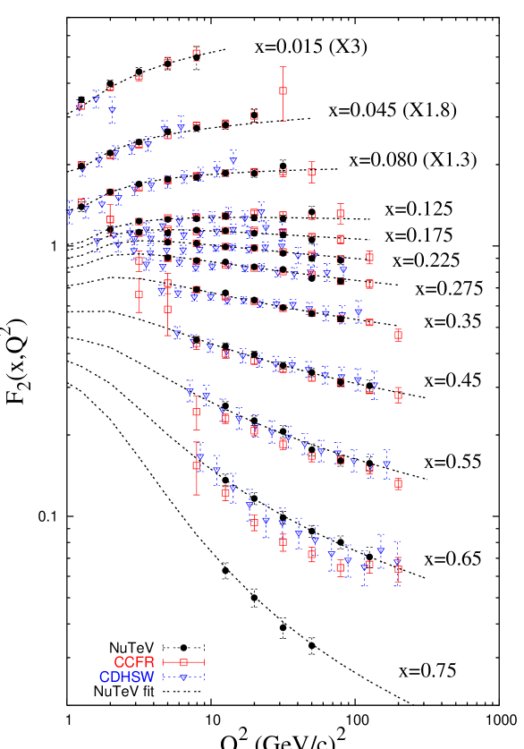
FIG. 9.: NuTeV measurement of $F_{2}(x,Q^{2})$ (solid circles) compared with previous $\nu$-Fe results; CCFR (open circles) and CDHSW (triangles). The data are corrected to an isoscalar (iron) target and for QED radiative effects as described in the text. The curve show the NuTeV model.

The difference of neutrino and anti-neutrino differential cross sections is proportional to the structure function $xF_{3}(x,Q^{2})$,

$$\frac{d^{2}\sigma^{\nu}}{dxdy}-\frac{d^{2}\sigma^{\overline{\nu}}}{dxdy}=\frac{2G_{F}^{2}ME}{\pi}\left[y-\frac{y^{2}}{2}\right]xF_{3}^{\scriptstyle AVG}(x,Q^{2})$$ (15)

where $xF_{3}^{\scriptstyle AVG}=\frac{1}{2}(xF_{3}^{\nu}+xF_{3}^{\overline{\nu}})$, and the difference between $F^{\nu}_{2}(x,Q^{2})$ and $F^{\overline{\nu}}_{2}(x,Q^{2})$ is assumed to be negligible. Figure 10 shows the NuTeV measurement of $xF_{3}(x,Q^{2})$ from fits to the cross section difference. The structure function, $xF_{3}(x,Q^{2})$ is compared with previous measurements from CDHSW [2] and CCFR97 [16].

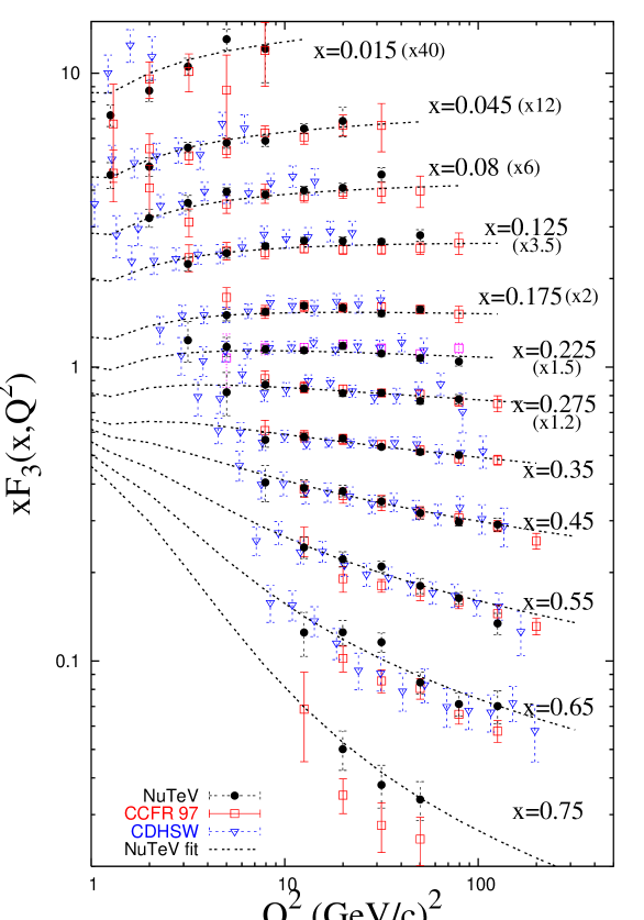
FIG. 10.: $xF_{3}(x,Q^{2})$ NuTeV (solid circles) compared with previous measurements; CCFR97 (open circles) and CDHSW (triangles). The data are corrected to an isoscalar (iron) target and for QED radiative effects as described in the text. The curve shows the NuTeV model.

V Data Comparisons

At moderate $x$, this result agrees well with CCFR over the full energy and $y$ range of the data, both in level and in shape, and agrees in level with CDHSW. The CDHSW measurement has a known $Q^{2}$ shape difference with CCFR [3], and thus also with this result. There are differences in NuTeV and CCFR at $x>0.40$ where CCFR’s measurement for both neutrino and antineutrino cross sections are consistently below our result for all energies. This is suprising since NuTeV used the refurbished CCFR detector and the analysis methods used by the two experiments were very similar. We discuss below several sources which may contribute to the high-$x$ cross section difference.

We have determined that the largest single contribution to the discrepancy is due to a mis-calibration of the magnetic field map of the toroid in CCFR. NuTeV performed thorough calibrations of muon and hadron responses in the detector, including mapping the response over the detector active area and measuring the energy scale over a wide range of energies [6]. This allowed NuTeV to measure precisely the radial dependence of the magnetic field in the toroid. Both experiments used the same muon spectrometer; therefore, the model of the magnetic field could have a different overall normalization, but the radial dependence (which is determined by the geometry of the muon spectrometer) should be the same for both. CCFR used one high statistics muon test beam run aimed at a single point in the spectrometer to set the absolute energy scale and modeled the radial dependence of the magnetic field using POISSON [17]. NuTeV used ANSYS to model the field and compared the prediction to a precision test beam map data. The width of the residual fractional difference distribution over the 45 test beam points is the main contribution to the absolute muon energy scale uncertainty (0.7%). If NuTeV uses the CCFR model the result is shifted to within 1.6 sigma agreement with CCFR at $x=0.65$. This accounts for 6% of the 18% difference at $x=0.65$. The field model differences can also be translated into an effective 0.8% difference in the muon energy scales by integrating the difference in the field models over the toroid.

The cross section model contributes an additional $\sim$3% to the discrepancy seen at x=0.65. Both experiments determine acceptance corrections using an iterated fit to the cross section data. Because the measured cross sections are different, this necessarily requires that the respective cross section models reflect the data differences. For example, the NuTeV model is above CCFR by $\sim 20\%$ at x=0.65. We have extracted cross sections using CCFR cross section model[3] and find that this contributes $\sim$3% to the discrepancy seen at x=0.65.

Other smaller sources for the difference come from muon and hadron energy smearing models which can also contribute to extracted cross section differences through acceptance corrections. We have determined that using the CCFR muon and hadron smearing models results in a difference of $\sim 2\%$ at $x=0.65$. In NuTeV the hadron energy response was found to have a small nonlinearity due to the shower $\pi^{0}$ fraction dependence on energy [6]. This nonlinearity was taken into account in NuTeV but not in CCFR. The effect of incorporating the hadron energy scale nonlinearity is small and contributes mainly to the $Q^{2}$ dependence.

All together these three contributions account for about two thirds of the high-$x$ cross section difference seen. This brings the two measurements within 1.2 sigma agreement in the high-$x$ region.

Another significant difference in the two experiments is that, while both used wide-band beams, NuTeV’s beam was sign-selected. In NuTeV, neutrino and anti-neutrino data were taken using separate high-purity beams. This allowed NuTeV to run the detector’s toroidal magnetic field polarity always set to focus the “right-sign” of muon produced in charged-current interactions. In CCFR, the beam had an 11% anti-neutrino component and neutrino and anti-neutrino data were taken simultaneously. The toroidal field polarity was reversed perodically to alternately focus either $\mu^{+}$ or $\mu^{-}$. To obtain adequate antineutrino statistics CCFR ran approximately half the time in focussing mode for each muon sign. This has two effects on the CCFR analysis that are not present in NuTeV. First, the acceptance corrections are different depending on whether the toroid is set to focus or defocus the muon. Second, in defocussing mode acceptance corrections are larger and consequently need to be more accurately determined. Acceptance falls off rapidly with $y$ at high-$x$, especially in defocussing mode where low-energy and wide-angle muons are deflected outward and spend less time the toroid magnetic field. CCFR had no test beam data for defocussing mode and, while acceptance corrections were modeled with a field simulation, the smearing model was assumed to be the same in both modes. We speculate that this difference may also contribute to the discrepancy seen.

VI Theory Comparisons

FIG. 11.: $F_{2}(x,Q^{2})$ fractional difference $\frac{F_{2}-F_{2}^{TRVFS}}{F_{2}^{TRVFS}}$ with respect to the TRVFS(MRST2001E) model. Data points are NuTeV (solid dots) and CCFR (open circles). Theory curves are ACOTFFS(CTEQ5HQ1) (solid line) and TRVFS(MRST2001E) $\pm 1\sigma$ (dashed lines). Theory curves are corrected for target mass and nuclear effects.

FIG. 12.: $xF_{3}(x,Q^{2})$ fractional difference $\frac{xF_{3}-xF_{3}^{TRVFS}}{xF_{3}^{TRVFS}}$ with respect to the TRVFS(MRST2001E) model. Data points are NuTeV (solid dots) and CCFR (open circles). Theory curves are ACOTFFS(CTEQ5HQ1) (solid line) and TRVFS(MRST2001E) $\pm 1\sigma$ (dashed lines). Theory curves are corrected for target mass and nuclear effects.

Figures 11 and 12 show a comparison of NuTeV and CCFR data with two theory models. The plot on Figure 11 shows the ratio of $F_{2}(x,Q^{2})$ to the Thorne-Roberts variable-flavor scheme (TRVFS) NLO QCD model [14] using the MRST2001 NLO $PDF$ set [18] for all $x$ bins. The $1\sigma$ error band from the $PDF$ set is also shown. The second theory curve shown on the plot is ACOT fixed-flavor scheme (ACOTFFS) NLO model [19] using CTEQ5HQ1 [20] $PDF$s. Similarily, the plot on Figure 12 shows the same comparison for $xF_{3}(x,Q^{2})$. All theory models have been corrected for target-mass effects using the Georgi-Politzer model [21]. These are important at high-$x$ and low-$Q^{2}$. For example, they increase the theory prediction by about 5% at $x=0.65$ and $Q^{2}=15$ GeV². To make a direct comparison, the theory curves are also corrected for nuclear target effects. A standard treatment of nuclear effects, which are not well determined for neutrino scattering, is to apply corrections measured in charged-leptons scattering from nuclear targets [4]. We use a multiplicative correction factor of the form [8]

$$f(x)=1.10-0.36x-0.28e^{-21.9x}+2.77x^{14.4}$$ (16)

obtained from a fit to charged-lepton scattering on nuclear targets. The correction is independent of $Q^{2}$ and is small at intermediate $x$ but is large at low and high $x$, (10% at $x=0.015$ and increases from 7% at $x=0.45$ to 15% at $x=0.65$).

The data show reasonable agreement with both the TRVFS(MRST2001E) and the ACOTFFS(CTEQ5HQ1) NLO QCD calculations for most of the $x$ and $Q^{2}$ range. At low $x$ ($x=0.015$ and $x=0.045$) both NuTeV and CCFR results have different $Q^{2}$ dependence than theoretical predictions. At high-$x$ ($x>0.5$) our data are systematically above the theory predictions. Compared with the TRVFS(MRST2001E) model the data are 15-20% high at $x=0.65$ and 25-40% at $x=0.75$. The data are about 10% higher at $x=0.65$ and 15% at $x=0.75$ than the ACOTFFS(CTEQ5HQ1) model prediction. The $Q^{2}$ dependence of the high-x data is similar to the prediction from the ACOTFFS(CTEQ5HQ1) model. A different theoretical treatment of nuclear effects could make a sizable difference at small and large $x$. NuTeV perhaps indicates that neutrino scattering favors smaller nuclear effects at high-$x$ than are found in charged-lepton scattering. At small $x$, new theoretical calculations show that in the shadowing region the nuclear correction has $Q^{2}$ dependence [22, 23]. The standard nuclear correction obtained from a fit to charged lepton data implies a suppression of 10% independent of $Q^{2}$ at $x=0.015$, while for $x=0.015$ reference [23] finds a suppression of 15% at $Q^{2}=1.25$GeV² and suppression of 3.4% at $Q^{2}=7.94$GeV². This effect somewhat improves agreement with data at low-$x$.

VII Data Access

The NuTeV neutrino and antineutrino cross sections and point-to-point covariance matrix can be downloaded from reference [24]. The tar file contains an unpacking routine and information on how to use the results.

NuTeV Cross Section Model

The NuTeV cross section model is inspired by the LO parameterization prescribed by Buras and Gaemers in reference [9]. The leading order model is modified to include non-leading order effects from $R_{L}$, higher-twist contributions, and the charm mass as described below. Because the quark densities used in the model are obtained from fits to neutrino-iron scattering data, no external model for nuclear effects is required to describe the NuTeV data. The cross section model described here is the ‘Born’-level neutrino DIS cross section for an isoscalar target. In addition, we correct for radiative effects using reference [12].

The neutrino isoscalar structure functions are given by

$$2xF_{1}(x,Q^{2}) = xu_{v}(x,Q^{2})+xd_{v}(x,Q^{2})$$ (17)

$$+ 2[xu_{s}(x,Q^{2})+xd_{s}(x,Q^{2})+xs_{s}(x,Q^{2})],$$ (18)

$$F_{2}(x,Q^{2}) = 2xF_{1}(x,Q^{2})\times\frac{1+R_{L}(x,Q^{2})}{1+4M^{2}x^{2}/Q^{2}},$$ (19)

$$xF_{3}(x,Q^{2}) = xu_{v}(x,Q^{2})+xd_{v}(x,Q^{2}).$$ (20)

The CKM matrix elements are used in the above formula to account for the mixing between the quarks, even though they are not shown here. $R_{L}(x,Q^{2})$ is obtained from an empirical fit to world data as described in reference [15]

$$R_{L}(x,Q^{2}) = \frac{0.0635}{{\rm ln}(Q^{2}/0.04)}\Theta(x,Q^{2})$$ (21)

$$+ \frac{0.5747}{Q^{2}}-\frac{0.3534}{Q^{4}+0.09},$$ (22)

$$\Theta(x,Q^{2}) = 1+12(\frac{Q^{2}}{1+Q^{2}})(\frac{0.125^{2}}{x^{2}+0.125^{2}}).$$ (23)

The charm production cross section is calculated using the slow rescaling model [4]. The Bjorken scaling variable, $x$, is rescaled

$$x\rightarrow\xi=x\cdot(1+\frac{m_{c}^{2}}{Q^{2}}).$$ (24)

The charm production differential cross section is suppressed by the factor $1-\frac{m_{c}^{2}}{2ME\xi}$. The value of the charm mass parameter used, $m_{c}=1.40\pm 0.18$, is obtained from the weighted average of leading-order experimental measurements [25],[26].

To account for higher-twist effects at high $x$ and low $Q^{2}$ an empirical model is used to constrain the $Q^{2}$ dependence of the $PDF$s by rescaling $x$ following reference [10].

$$x\rightarrow\xi_{HT}=x\frac{Q^{2}+B_{HT}}{Q^{2}+A_{HT}\cdot x},$$ (25)

where $A_{HT}$ and $B_{HT}$ are fit parameters in the model. The shape of GRV94L0 [11] $PDF$s is used to extrapolate the model for $Q^{2}<1.35GeV^{2}/c^{2}$. The normalizations are constrained by matching the $PDF$s to the Buras-Gaemers $PDF$s at $Q^{2}=1.35GeV^{2}/c^{2}$.

The form for the parton distribution functions follow the Buras-Gaemers parameterization in reference [9]. The valence distributions are given by

$$xu_{v}(x) = u_{tot}\times[x^{E_{1}}(1-x)^{E_{2}}+AV_{2}x^{E_{3}}(1-x)^{E_{4}}]$$ (26)

$$xd_{v}(x) = d_{tot}\times xu_{v}(x)\times(1-x),$$ (27)

with parameters $AV_{2}$, $E_{1}$, $E_{2}$, $E_{3}$, and $E_{4}$. The $Q^{2}$-dependence for the valence is given by

$$E_{i} = E_{i0}+E_{i1}\cdot s,i=1,4$$ (28)

$$s = {\rm ln}\left[\frac{{\rm ln}(\frac{Q^{2}}{A_{0}^{2}})}{{\rm ln}(\frac{Q_{0}^{2}}{A_{0}^{2}})}\right]$$ (29)

where the reference $Q_{0}^{2}$ is set to 12.6 $GeV^{2}/c^{2}$ and the QCD scale, $A_{0}$, is a parameter in the fit.

The constraints on the valence distributions include the normalization of the valence densities, which is determined from a variant of the Gross-Llewllyn-Smith sum rule, and the relative normalization between $u_{v}$ and $d_{v}$, which is determined from quark counting

$$\int_{0}^{1}xF_{3}(x,Q^{2})dx = 3\Big{(}1-\frac{\alpha_{s}(Q^{2})}{\pi}\Big{)}$$ (30)

$$= 3\Big{(}1-\frac{A1}{{\rm log}(Q^{2}/A_{0}^{2})}-\frac{A2}{\left[{\rm log}(Q^{2}/A_{0}^{2})\right]^{2}}\Big{)}$$ (31)

$$\int_{0}^{1}u_{v}(x,Q^{2})dx = 2\Big{(}1-\frac{A1}{{\rm log}(Q^{2}/A_{0}^{2})}-\frac{A2}{\left[{\rm log}(Q^{2}/A_{0}^{2})\right]^{2}}\Big{)}$$ (32)

$$\int_{0}^{1}d_{v}(x,Q^{2})dx = \Big{(}1-\frac{A1}{{\rm log}(Q^{2}/A_{0}^{2})}-\frac{A2}{\left[{\rm log}(Q^{2}/A_{0}^{2})\right]^{2}}\Big{)}$$ (33)

In addition a charge constraint is required

$$\frac{2}{3}\int_{0}^{1}u_{v}(x,Q^{2})dx - \frac{1}{3}\int_{0}^{1}d_{v}(x,Q^{2})dx$$ (34)

$$= \Big{(}1-\frac{A1}{{\rm log}(Q^{2}/A_{0}^{2})}-\frac{A2}{\left[{\rm log}(Q^{2}/A_{0}^{2})\right]^{2}}\Big{)},$$ (35)

where the fit parameters $A1$ and $A2$ describe the normalization of the leading order and next-to-leading order terms respectively.

The light quark sea distributions are given by

$$x\overline{u}(x) = x\overline{d}(x)=\frac{1}{2(\kappa+2)}xS(x)$$ (36)

$$= \frac{1}{2(\kappa+2)}(AS(1-x)^{ES}+AS_{2}(1-x)^{ES_{2}}),$$ (37)

where $S(x)$ is the light-quark sea density. $AS$, $AS_{2}$, $ES$, and $ES_{2}$ are defined in terms of fit parameters below, and the parameter $\kappa$ is the relative normalization to the strange sea, also defined below. The light quark sea distributions can be determined from the first two moments, because they decrease rapidly with x

$$S_{2} = \int_{0}^{1}xSdx=\frac{3}{4}D_{22}+\frac{1}{4}D_{12},$$ (38)

$$S_{3} = \int_{0}^{1}x^{2}Sdx=\frac{3}{4}D_{23}+\frac{1}{4}D_{13},$$ (39)

where the values for $D_{ij}$, which are completely specified by LO QCD, are given in [9]. $AS_{2}$ and $ES_{2}$ are evolved with $Q^{2}$ in the following way

$$AS_{2} = AS_{20}+AS_{21}{\rm ln}(Q^{2}),$$ (40)

$$ES_{2} = ES_{20}+ES_{21}{\rm ln}(Q^{2}).$$ (41)

$S_{2}$, $S_{3}$, $AS_{20}$, $AS_{21}$, $ES_{20}$, and $ES_{21}$ are parameters in the fit. $AS$ and $ES$ are constrained to match the moments $S_{2}$ and $S_{3}$.

$$ES = \frac{S_{2}-AS_{2}/(ES_{2}+1)}{S_{3}-AS2/((ES_{2}+1)(ES_{2}+2))}-2,$$ (42)

$$AS = (ES+1)\frac{S_{2}-AS_{2}}{ES_{2}+1}.$$ (43)

The strange sea distribution can be measured from the dimuon inclusive cross section. The parameterization of the strange sea is a LO fit to the CCFR dimuon differential cross section [25],

$$xs(x) = x\overline{s}(x)=\frac{\kappa}{2(\kappa+2)}xSS(x)$$ (44)

where $SS(x)$ is the strange sea density. The relative normalization to the light quark seas is determined by the parameter $\kappa$,

$$xs(x)\propto\kappa\frac{x\overline{u}_{R}(x)+x\overline{d}_{R}(x)}{2}(1-x)^{\alpha},$$ (46)

where $\alpha$ describes the shape of the strange sea. Here the light quark sea densities $\overline{u}_{R}(x)$ and $\overline{d}_{R}(x)$, and the values of $\alpha=2.5$ and $\kappa=0.373$ are obtained from reference [25].

Momentum sum rule is constrained by the second moment of the gluon distribution $G_{2}=\int_{0}^{1}xg(x,Q^{2})dx$

$$G_{2} + \int_{0}^{1}\frac{1+R(x,Q^{2})}{1+4M^{2}x^{2}/Q^{2}}[xu_{v}(x,Q^{2})$$ (47)

$$+ xd_{v}(x,Q^{2})+xS(x,Q^{2})]dx=1$$ (48)

Additional small corrections are used to modify $u$ and $d$ distributions to account for the $u,d$ asymmetry observed in muon DIS and Drell-Yan data. Drell-Yan data from E866 [27] is used to constrain the $\overline{u},\overline{d}$ asymmetry by the factor

$$f(\overline{d}/\overline{u}) = \frac{1}{{\rm max}(1-x(2.7-0.14{\rm ln}(Q^{2})-1.9x),0.1)}$$ (49)

The modified light sea distributions $\overline{u^{\prime}},\overline{d^{\prime}}$ are constrained by $\overline{u^{\prime}}+\overline{d^{\prime}}=\overline{u}+\overline{d}$ and have the form

$$\overline{u^{\prime}} = \overline{u}\left(\frac{\overline{u}+\overline{d}}{\overline{u}+\overline{d}\cdot f(\overline{d}/\overline{u})}\right),$$ (50)

$$\overline{d^{\prime}} = \overline{d}\left(\frac{\overline{u}+\overline{d}}{\overline{u}+\overline{d}\cdot f(\overline{d}/\overline{u})}\right)\cdot f(\overline{d}/\overline{u}).$$ (51)

The valence distributions are also modified for the $u_{v},d_{v}$ asymmetry. The modified valence distributions $u_{v}^{\prime},d_{v}^{\prime}$ are constrained by $u_{v}^{\prime}+d_{v}^{\prime}=u_{v}+d_{v}$ and have the form [3]

$$u_{v}^{\prime} = \frac{u_{v}}{1+\delta(d/u)\cdot u_{v}/(u_{v}+d_{v})},$$ (52)

$$d_{v}^{\prime} = \frac{d_{v}+u_{v}\cdot\delta(d/u)}{1+\delta(d/u)\cdot u_{v}/(u_{v}+d_{v})},$$ (53)

$$\delta(d/u) = 0.12079-1.3303x+4.9829x^{2}$$ (54)

$$- 8.4465x^{3}+5.7324x^{4}.$$ (55)

The model fit parameters are obtained after an iterative loop in which the $n^{th}$ loop flux and cross section are re-extracted with the $(n-1)^{th}$ loop model fit parameters. The $n^{th}$ loop model then determines new acceptance and smearing corrections which are used for the $(n+1)^{th}$ cross section and fit. New radiative corrections are computed to correspond to each new model. The initial flux and cross section are determined using a starting model with the Buras-Gaemers $PDF$ parameters from the best fit to CCFR data [3]. The process is iterated until the average relative change in the cross section data points compared to the previous iteration is less than 0.1% (within 3 iterations).

To constrain the high-$x$ and low $Q^{2}$ part of the model, which is important in order to model our flux data sample, we include data from charged-lepton scattering in the fit. The SLAC [28], BCDMS [29], and NMC [30] overlap with the kinematic range of our data set but extend to lower-$Q^{2}$. The charged-lepton data for $x$ in the range $0.4<x<0.7$, are included in the fit $\chi^{2}$ function along with the NuTeV data set to determine the best fit parameters. The charged-lepton data must first be corrected to $F_{2}^{\nu}$ using our model and corrected to an $A=56$ iron target using Equation 16. The normalization of the charged-lepton data relative to the NuTeV data is unconstrained in the fit.

Table I gives the NuTeV cross section model fit values for each parameter and their estimated uncertainties. A total of 19 parameters are fit in the model. Note that we do not expect that the parameterization extrapolated beyond the region of the NuTeV data set will be a good description of data there.

TABLE I.: The final fit parameters for the NuTeV cross section model.

Parameter	Value	Estimated Error
$A_{0}$	0.583	0.017
$A_{1}$	0.295	0.013
$A_{2}$	0.17	0.03
$E_{10}$	0.5333	0.0025
$E_{11}$	-0.028	0.011
$E_{20}$	2.61	0.015
$E_{21}$	1.31	0.045
$AV_{2}$	637.0	75.0
$E_{30}$	4.56	0.14
$E_{40}$	12.5	0.35
$S_{2}$	0.1625	0.0013
$S_{3}$	0.0159	0.0004
$G_{3}$	0.031	0.003
$AS_{20}$	1.06	0.11
$AS_{21}$	1.76	0.25
$ES_{20}$	185.0	20.0
$ES_{21}$	8.4	8.0
$A_{HT}$	1.187	0.035
$B_{HT}$	0.33	0.02

REFERENCES

- [1] V. Barone, C. Pascaud, F. Zomer, Eur. Phys. J. C12 (2000) 243.
- [2] P. Berge et. al, Z. Phys. C49 (1991) 187.
- [3] U. K. Yang, Ph. D. Thesis, University of Rochester, (2001), UR-1583.
- [4] J. Conrad, M. H. Shaevitz, and T. Bolton, Rev. Mod. Phys. 70 (1998) 4.
- [5] G. Sterman et. al, Rev. Mod. Phys. 67 (1995) 157.
- [6] D. A. Harris et. al, Nucl. Instrum. Methods A447 (2000) 377.
- [7] Finite element analysis software, http://www.ansys.com.
- [8] W. Seligman, Ph. D. Thesis, Columbia University, Nevis 292 (1997).
- [9] A. J. Buras and K. L. F. Gaemers, Nucl. Phys. B132 (1978) 2109.
- [10] A. Bodek and U. K. Yang, Nucl. Phys. Proc. Suppl. 112 (2002) 70.
- [11] M. Gluck et. al (GRV collaboration), Z. Phys. C67, 433 (1995).
- [12] D. Y. Bardin and V. A. Dokuchaeva, JINR-E2-86-260 (1986).
- [13] Arie Bodek, Inkyu Park, Un-ki Yang, Nucl. Phys. Proc. Suppl. 139 (2005) 113-118. [arXiv:hep-ph/0411202].
- [14] R. Thorne and R. Roberts, Phys. Lett. B421 (1998) 303. A. D. Martin et. al. Eur. Phys. J. C18 (2000) 117.
- [15] L. W. Whitlow et. al, Phys. Lett. B250 (1990) 193.
- [16] W. G. Seligman et. al, Phys. Rev. Lett. 79 (1997) 1213.
- [17] CERN computer program POISSON; see R. Holsinger, CERN Computer Center Program Library T604.
- [18] A. D. Martin, R. G. Roberts, W. J. Stirling, R. S. Thorne, Eur. Phys. J. C28 (2003) 455-473.
- [19] M. A. G. Aivazis, J. C. Collins, F. I. Olness, and W. K. Tung, Phys. Rev. D50, 3102 (1994).
- [20] H. L. Lai et. al., Eur. Phys. J. C12 (2000) 375-392.
- [21] H. Georgi and H. D. Politzer, Phys. Rev. D14 (1976) 1829.
- [22] S.A. Kulagin, R. Petti, [arXiv:hep-ph/0412425].
- [23] J. W. Qiu and I. Vitev, Phys. Lett. B587, (2004) 52 [arXiv:hep-ph/0401062].
- [24] http://www-nutev.phyast.pitt.edu/results2005/nutevsf.html.
- [25] S. Rabinowitz et. al, Phys. Rev. Lett. 70 (1993) 134.
- [26] P. Vilain et. al, Eur. Phys. J. C11 (1999) 19; P. Astier et. al, Phys. Lett. B486 (2000) 35.
- [27] A. Hawker et. al, Phys Rev Lett 80 (1998) 3715.
- [28] L. W. Whitlow et. al, Phys. Lett. B282 (1992) 475.
- [29] A. C. Benvenuti et. al, Phys. Lett. B223 (1989) 485; A. C. Benvenuti et. al, Phys. Lett. B236 (1989) 592.
- [30] M. Arneodo et. al, Nucl. Phys. B483 (1997) 3.