Search for $\Lambda_{c}^{+}\to\mbox{{p}}\mbox{{K}}^{+}\pi^{-}$ and $\mbox{{D}}_{s}^{+}\to\mbox{{K}}^{+}\mbox{{K}}^{+}\pi^{-}$ Using Genetic Programming Event Selection

Abstract

We apply a genetic programming technique to search for the doubly Cabibbo suppressed decays $\Lambda_{c}^{+}\to\mbox{{p}}\mbox{{K}}^{+}\pi^{-}$ and $\mbox{{D}}_{s}^{+}\to\mbox{{K}}^{+}\mbox{{K}}^{+}\pi^{-}$. We normalize these decays to their Cabibbo favored partners and find $\text{BR}(\Lambda_{c}^{+}\to\mbox{{p}}\mbox{{K}}^{+}\pi^{-})/\text{BR}(\Lambda_{c}^{+}\to\mbox{{p}}\mbox{{K}}^{-}\pi^{+})=(0.05\pm 0.26\pm 0.02)\%$ and $\text{BR}(\mbox{{D}}_{s}^{+}\to\mbox{{K}}^{+}\mbox{{K}}^{+}\pi^{-})/\text{BR}(\mbox{{D}}_{s}^{+}\to\mbox{{K}}^{-}\mbox{{K}}^{+}\pi^{+})=(0.52\pm 0.17\pm 0.11)\%$ where the first errors are statistical and the second are systematic. Expressed as $90\%$ confidence levels (CL), we find $<0.46\%$ and $<0.78\%$ respectively. This is the first successful use of genetic programming in a high energy physics data analysis.

Cabibbo suppressed (CS) and doubly Cabibbo suppressed (DCS) decays are important in helping us understand the dynamics of hadronic decay processes. DCS decays are unique to the charmed hadrons; charm is the only heavy up-type quark that hadronizes. DCS decay rates are such that only DCS decays of $\mbox{{D}}^{+}$ and $\mbox{{D}}{}^{0}$ have been observed, while CS decays of nearly all the charmed hadrons have been observed. This paper presents a search for DCS decays of $\Lambda_{c}^{+}$ and $\mbox{{D}}_{s}^{+}$. Both branching ratios are expected to be small. Naïve expectations place DCS branching ratios around $\tan^{4}\theta_{c}$, or about 0.25%, relative to their Cabibbo favored (CF) counterparts. Lipkin argues [1] that exact SU(3) symmetry would require the product of the DCS relative branching ratios $\text{BR}(\mbox{{D}}^{+}\to\mbox{{K}}^{+}\pi^{-}\pi^{+})/\text{BR}(\mbox{{D}}^{+}\to\mbox{{K}}^{-}\pi^{+}\pi^{+})$ and $\text{BR}(\mbox{{D}}_{s}^{+}\to\mbox{{K}}^{+}\mbox{{K}}^{+}\pi^{-})/\text{BR}(\mbox{{D}}_{s}^{+}\to\mbox{{K}}^{-}\mbox{{K}}^{+}\pi^{-})$ to be exactly $\tan^{8}\theta_{c}$. This means the latter should be about 0.07%; a much larger value requires a large violation of flavor SU(3). In the $\Lambda_{c}^{+}$ case, the CF normalizing mode has a c-d $\mbox{{W}}^{+}$ exchange decay channel available, while the DCS decay mode may only proceed through spectator decays. The lifetime difference between $\Lambda_{c}^{+}$ and $\Xi_{c}^{+}$ shows us that this exchange mode is important, so we expect that the branching ratio for $\Lambda_{c}^{+}\to\mbox{{p}}\mbox{{K}}^{+}\pi^{-}$ should also be less than $\tan^{4}\theta_{c}$.

We have applied a genetic programming (GP) [2] technique to search for the DCS decays $\mbox{{D}}_{s}^{+}\to\mbox{{K}}^{+}\mbox{{K}}^{+}\pi^{-}$ and $\Lambda_{c}^{+}\to\mbox{{p}}\mbox{{K}}^{+}\pi^{-}$ (charge-conjugate states are implied), neither of which have been observed. GP is a machine learning technique which evolves populations of programs (event filters in our case) over a series of generations. The genetic programming learning mechanism is modeled on biological and evolutionary principals and differs from some other machine learning solutions in that the form of the solution is not specified in advance but is determined by the complexity of the problem. A full demonstration of this technique on the observed DCS decay $\mbox{{D}}^{+}\to\mbox{{K}}^{+}\pi^{+}\pi^{-}$ is given in Reference 3.

These results use data taken with the charm photoproduction experiment FOCUS (FNAL-E831), an upgraded version of FNAL-E687 [4] which collected data using the Wideband photon beamline during the 1996–1997 Fermilab fixed-target run. The FOCUS experiment utilizes a forward multiparticle spectrometer to study charmed particles produced by the interaction of high energy photons ($\langle E\rangle\approx 180~{}\mathrm{GeV}$) [5] with a segmented BeO target. Charged particles are tracked within the spectrometer by two silicon microvertex detector systems. One system is interleaved with the target segments [6]; the other is downstream of the target region. These detectors provide excellent separation of the production and decay vertices. Further downstream, charged particles are tracked and momentum analyzed with a system of five multiwire proportional chambers [7] and two dipole magnets of opposite polarity. Three multicell threshold Čerenkov detectors are used to identify electrons, pions, kaons, and protons. FOCUS also contains a complement of hadronic and electromagnetic calorimeters and muon detectors.

We use loose analysis cuts on both DCS and CF decay modes to select initial samples of events for optimization by GP. The FOCUS Čerenkov algorithm [8] returns negative $2\times\text{log-likelihood}$ values $W_{i}(j)$ for particle $j$ and hypothesis $i\in{e,\pi,K,p}$. Differences between log-likelihoods are used as particle ID, such as $\Delta W_{Kp}(p)\equiv W_{K}(p)-W_{p}(p)$ for “proton favored over kaon.” We require $\Delta W_{\pi K}(K)>2$ for all kaons in both decay modes. For protons from $\Lambda_{c}^{+}$ candidates, we require $\Delta W_{\pi p}(p)>4$ and $\Delta W_{Kp}(p)>0$ in the initial selection. For the $\Lambda_{c}^{+}$, we also require that the separation between the production and decay vertices, $\ell$, is greater than 3 times its error, $\sigma_{\ell}$. For the $\mbox{{D}}_{s}^{+}$, the vertex separation requirement is $\ell/\sigma_{\ell}>6$. For both $\Lambda_{c}^{+}$ and $\mbox{{D}}_{s}^{+}$, the three decay fragments must form a vertex with a confidence level (CL) $>1\%$, and a production vertex is formed by adding as many remaining tracks to the charm candidate as possible while maintaining a vertex CL $>1\%$. One additional requirement is placed on the CF (DCS) $\mbox{{D}}_{s}^{+}$ candidates: the $K^{-}K^{+}\pi^{+}$ ($K^{+}K^{+}\pi^{-}$) combination is rejected if, reconstructed as $K^{-}\pi^{+}\pi^{+}$ ($K^{+}\pi^{+}\pi^{-}$), the mass is within $2\sigma$ of the nominal $\mbox{{D}}^{+}$ mass. This cut removes a prominent reflection from the CF candidates and stabilizes the many fits done during the optimization process; it is applied to the DCS mode for consistency. The initial samples of $\Lambda_{c}^{+}$ and $\mbox{{D}}_{s}^{+}$ candidates in CF and DCS decay modes are shown in Fig. 1.

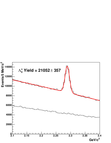
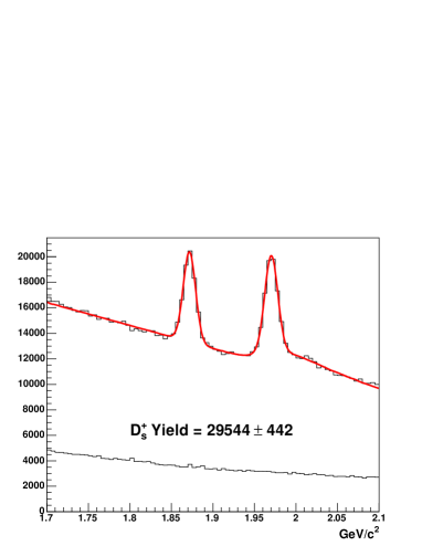
Figure 1: Initial $\Lambda_{c}^{+}$ (left) and $\mbox{{D}}_{s}^{+}$ (right) data samples. The upper distributions show the CF decay candidates, the lower distributions show the DCS candidates. In the $\mbox{{D}}_{s}^{+}$ plot, the $\mbox{{D}}^{+}\to\mbox{{K}}^{-}\pi^{+}\pi^{+}$ rejection cut described in the text is not applied and a contribution to the fit for this reflection is visible to the right of the $\mbox{{D}}_{s}^{+}$ peak.

A GP framework (GPF) evolves and tests event filters. For each filter, we define a fitness

$$f\propto\frac{B_{\text{DCS}}}{S_{\text{CF}}^{2}}\times(1+0.005\times N_{\text{nodes}})$$ (1)

where $B_{\text{DCS}}$ is the number of background events found in a fit of the DCS mass distribution which excludes the signal region, and $S_{\text{CF}}$ is the fitted CF yield. $S_{\text{CF}}/\sqrt{B_{\text{DCS}}}$ is proportional to the projected DCS significance assuming no real DCS events and equal CF and DCS selection efficiencies; squaring this quantity further emphasizes “better” filters and inverting it allows small fitnesses to describe good event filters. $N_{\text{nodes}}$ is the total number of variables, constants, functions, and operators used in the filter and is included as a penalty term to encourage smaller filters and to attempt to eliminate the addition of nodes which do not select events based on physics.

For the data samples in Fig. 1, half the events (as explained later) along with a large number of variables (37 for $\Lambda_{c}^{+}$, 34 for $\mbox{{D}}_{s}^{+}$), operators and functions (21), and constants are used as inputs to the GPF which randomly generates a large number of filters and calculates the fitness of each. The GPF preferentially selects filters for which this fitness is small to participate in breeding subsequent generations of filters. In this way subsequent generations develop filters with better average fitnesses. At the end of the process we use the filter with the single best fitness to select events for further analysis.

The variables and resulting filter used in the CF and DCS decays are identical. All variables commonly used in FOCUS analyses and some additional variables are allowed to be used in the event filter. These can be roughly broken into categories of vertexing, track quality, particle identification, production and decay kinematics, away-side charm tagging and, for the $\Lambda_{c}^{+}$, evidence for decays of the excited states $\Sigma_{c}^{(*)0,++}$. A description of the variables used, examples of the event filters constructed, and how the population of filters evolves over many generations can be found in Reference 3. In both cases we use 20 sub-populations of 1500 event filters per generation as described in Reference 3.

When searching for $\Lambda_{c}^{+}\to\mbox{{p}}\mbox{{K}}^{+}\pi^{-}$ and $\mbox{{D}}_{s}^{+}\to\mbox{{K}}^{+}\mbox{{K}}^{+}\pi^{-}$ decays (with the signal regions masked), the GPF is allowed to run for 80 generations. The process is terminated when no improvement in fitness is observed for about 10 generations. The best $\Lambda_{c}^{+}\to\mbox{{p}}\mbox{{K}}^{+}\pi^{-}$ filter found has 45 nodes and uses 12 unique physics variables. The events selected are shown in Fig. 2. One can see that about 15% of the signal is retained compared to Fig. 1 while the backgrounds are reduced by a factor of $\sim$1000. The distributions in both the CF and DCS cases are fit with a second degree polynomial and a single Gaussian. In the DCS case, the Gaussian mean and $\sigma$ are fixed to the CF values and we find $1.2\pm 6.6$ events. Correcting for the relative efficiency $\epsilon_{\text{CF}}/\epsilon_{\text{DCS}}=1.204\pm 0.007$ (stat.) calculated with Monte Carlo (MC) simulations, we obtain a relative BR of

$$\frac{\text{BR}(\Lambda_{c}^{+}\to\mbox{{p}}\mbox{{K}}^{+}\pi^{-})}{\text{BR}(\Lambda_{c}^{+}\to\mbox{{p}}\mbox{{K}}^{-}\pi^{+})}=(0.05\pm 0.26)\%\,,$$ (2)

which is consistent with zero.

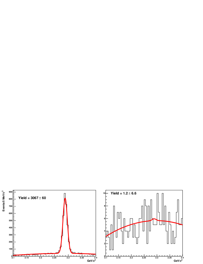
Figure 2: $\Lambda_{c}^{+}$ samples after selection. On the left is the CF normalizing mode, on the right, the remaining $\Lambda_{c}^{+}\to\mbox{{p}}\mbox{{K}}^{+}\pi^{-}$ candidates.

The best $\mbox{{D}}_{s}^{+}\to\mbox{{K}}^{+}\mbox{{K}}^{+}\pi^{-}$ filter found has 85 nodes and uses 15 unique physics variables. The events selected are shown in Fig. 3. The fits shown are performed identically to the $\Lambda_{c}^{+}$ case except that an additional Gaussian is added to the CF distribution for the CS decay $\mbox{{D}}^{+}\to\mbox{{K}}^{-}\mbox{{K}}^{+}\pi^{+}$. We find $27.5\pm 9.2$ events in the DCS distribution which, corrected by the relative efficiency $\epsilon_{\text{CF}}/\epsilon_{\text{DCS}}=1.154\pm 0.005$, gives a relative BR of

$$\frac{\text{BR}(\mbox{{D}}_{s}^{+}\to\mbox{{K}}^{+}\mbox{{K}}^{+}\pi^{-})}{\text{BR}(\mbox{{D}}_{s}^{+}\to\mbox{{K}}^{-}\mbox{{K}}^{+}\pi^{+})}=(0.52\pm 0.17)\%\,.$$ (3)

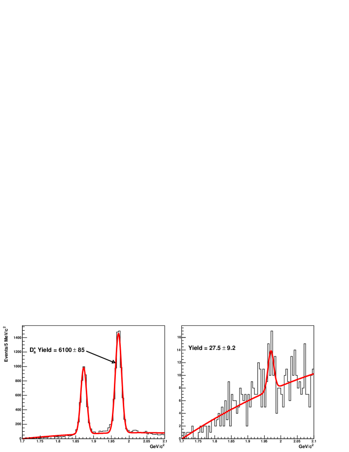
Figure 3: $\mbox{{D}}_{s}^{+}$ samples after selection. On the left is the CF normalizing mode, on the right, the remaining $\mbox{{D}}_{s}^{+}\to\mbox{{K}}^{+}\mbox{{K}}^{+}\pi^{-}$ candidates.

In both cases our central values are calculated assuming non-resonant decays for the DCS case and the best known resonance models for the CF decays (the PDG [9] model for $\Lambda_{c}^{+}$ and a FOCUS model for $\mbox{{D}}_{s}^{+}$) as explained below.

To convert these relative BRs into upper limits including systematic errors, we use a method proposed by Convery [10] for incorporating systemic uncertainties on reconstruction efficiencies into BR measurements when a fit, rather than event counting, is used. In this case, the probability $P(B)$ of the true BR being $B$ is given by

$$p(B)\propto\frac{1}{\sqrt{\frac{B^{2}}{2\sigma_{B}^{2}}+\frac{\hat{S}^{2}}{2\sigma_{S}^{2}}}}\,\exp\left[\frac{-(B-\hat{B})^{2}}{2\left(\frac{B^{2}\sigma_{S}^{2}}{\hat{S}^{2}}+\sigma_{B}^{2}\right)}\right]$$ (4)

where $\hat{B}$ is the fitted BR, $\sigma_{B}$ is its error and $\sigma_{S}/\hat{S}$ is the percent systematic error on the efficiency. $P(B)$ is numerically integrated until the point at which 90% of the physical $(\textrm{BR}>0)$ area is included. This point is reported as the 90% confidence level. If $\sigma_{S}/\hat{S}\gg 10\%$, this distribution has a long high-end tail, raising the 90% limit considerably.

We consider four sources of systematic error on our knowledge of the relative efficiencies of the CF and DCS decay modes. First, and negligible, is the number of MC events used. Second and third, we consider the effects of different resonance models for the DCS and CF states respectively. Finally, we consider whether the evolved event selector may have different efficiencies for the CF and DCS modes.

In studying possible resonances for $\Lambda_{c}^{+}\to\mbox{{p}}\mbox{{K}}^{+}\pi^{-}$ candidates, we calculate efficiencies as if the final state is entirely non-resonant or entirely $\Lambda_{c}^{+}\to\Delta(1232)^{0}\mbox{{K}}^{+}$ or $\Lambda_{c}^{+}\to\mbox{{p}}\mbox{{K}}^{*}(892)^{0}$. The systematic error is taken as the standard deviation of the three possible efficiencies. For the $\mbox{{D}}_{s}^{+}\to\mbox{{K}}^{+}\mbox{{K}}^{+}\pi^{-}$ candidates, we consider non-resonant decays, $\mbox{{D}}_{s}^{+}\to\mbox{{K}}^{*}(892)^{0}\mbox{{K}}^{+}$, and $\mbox{{D}}_{s}^{+}\to\mbox{{K}}^{*}_{0}(1430)^{0}\mbox{{K}}^{+}$ in the same way. From these studies we find 5.3% and 10.7% systematic uncertainties on the $\Lambda_{c}^{+}$ and $\mbox{{D}}_{s}^{+}$ efficiencies respectively.

The resonant structures of the CF decays are reasonably well known. For the $\Lambda_{c}^{+}$, we use two models, one from the PDG and another which excludes the $\Lambda(1520)^{0}\pi^{+}$ decay mode. For the $\mbox{{D}}_{s}^{+}$, we consider an incoherent model based on the PDG averages and a coherent model [11] developed from the FOCUS data. From these studies we find 2.1% and 2.6% uncertainties on the $\Lambda_{c}^{+}\to\mbox{{p}}\mbox{{K}}^{-}\pi^{+}$ and $\mbox{{D}}_{s}^{+}\to\mbox{{K}}^{-}\mbox{{K}}^{+}\pi^{+}$ efficiencies, respectively.

Our final systematic contribution is motivated by the concern that the efficiency of the final GP-generated event filter may differ for the CF and DCS modes (after correction for kinematic acceptance of different final states) in a way that is not well modeled by MC. Since this is impossible to measure, we adopt a more rigorous test. We test if the event filter has the same efficiency on CF data and MC events. We do this by comparing the CF yields of data and MC samples before and after the event filter is applied. For the $\Lambda_{c}^{+}$, we find that the event filter retains $14.5\pm 0.4\%$ and $14.9\pm 0.1\%$ of the data and MC events, respectively. For the $\mbox{{D}}_{s}^{+}$, we determine these quantities to be $21.0\pm 0.4\%$ and $20.3\pm 0.1\%$. We take the differences between these numbers (neglecting the errors) as systematic uncertainties; these cause 2.6% and 3.5% uncertainties on the relative efficiencies for $\Lambda_{c}^{+}\to\mbox{{p}}\mbox{{K}}^{+}\pi^{-}$ and $\mbox{{D}}_{s}^{+}\to\mbox{{K}}^{+}\mbox{{K}}^{+}\pi^{-}$ respectively. All systematic uncertainties on the relative efficiencies are summarized in Table 1.

Table 1: Summary of systematic uncertainties. Listed are the percent uncertainties on the relative efficiencies of the DCS and CF decay modes from various sources.

	Syst. Unc. (%)
Source	$\Lambda_{c}^{+}$	$\mbox{{D}}_{s}^{+}$
MC statistics	0.6	0.4
DCS resonances	5.3	10.7
CF resonances	2.1	2.6
GP filter	2.6	3.5
Total	6.3	11.6

Finally, as mentioned above, we only use half (even-numbered) of the events in the optimization of the event filter. The final values use the event filter applied to all the events, but as a check, we divide the sample into events the GPF used and did not use. We measure the BR independently for these two samples and see no significant evidence for a difference, strongly suggesting that the GPF is not arbitrarily selecting or rejecting small numbers of events to artificially reduce backgrounds or enhance signals.

Using the total percent errors in Table 1 as $\sigma_{S}/\hat{S}$ and the above BRs, statistical errors, and percent systematic errors, we integrate $P(B)$ from Eq. 4 as described and find

$$\frac{\text{BR}(\Lambda_{c}^{+}\to\mbox{{p}}\mbox{{K}}^{+}\pi^{-})}{\text{BR}(\Lambda_{c}^{+}\to\mbox{{p}}\mbox{{K}}^{-}\pi^{+})}<0.46\%$$ (5)

and

$$\frac{\text{BR}(\mbox{{D}}_{s}^{+}\to\mbox{{K}}^{+}\mbox{{K}}^{+}\pi^{-})}{\text{BR}(\mbox{{D}}_{s}^{+}\to\mbox{{K}}^{-}\mbox{{K}}^{+}\pi^{+})}<0.78\%$$ (6)

where the limits are at the 90% CL. We also determine effective systematic uncertainties for our measurements by calculating the uncertainty necessary, when added in quadrature to the statistical uncertainty, to cover the central 68% of the distrubution in Eq. 4. By this method, we find $\text{BR}(\Lambda_{c}^{+}\to\mbox{{p}}\mbox{{K}}^{+}\pi^{-})/\text{BR}(\Lambda_{c}^{+}\to\mbox{{p}}\mbox{{K}}^{-}\pi^{+})=(0.05\pm 0.26\pm 0.02)\%$ and $\text{BR}(\mbox{{D}}_{s}^{+}\to\mbox{{K}}^{+}\mbox{{K}}^{+}\pi^{-})/\text{BR}(\mbox{{D}}_{s}^{+}\to\mbox{{K}}^{-}\mbox{{K}}^{+}\pi^{+})=(0.52\pm 0.17\pm 0.11)\%$ where the first errors are statistical and the second are systematic. The distributions described by Eq. 4 and the 90% integrals for the DCS decays are shown in Fig. 4. Both limits are larger than the expected ($\lesssim\tan^{4}\theta_{c}$) level, but are the first reported limits on these decays. Furthermore, this is the first successful application of the GP technique to an HEP data analysis.

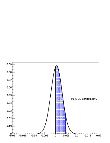
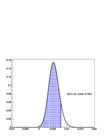
Figure 4: Relative BR limit determination for $\Lambda_{c}^{+}\to\mbox{{p}}\mbox{{K}}^{+}\pi^{-}$ (left) and $\mbox{{D}}_{s}^{+}\to\mbox{{K}}^{+}\mbox{{K}}^{+}\pi^{-}$ (right). The curves show the branching ratio probability for DCS decays relative to CF decays. The vertical axes are arbitrary. The shaded areas show the 90% integrals over the physical range.

References

- [1] H. J. Lipkin, Puzzles in hyperon, charm and beauty physics, Nucl. Phys. Proc. Suppl. 115 (2003) 117–121.
- [2] J. R. Koza, Genetic Programming: On the Programming of Computers by Means of Natural Selection, The MIT Press, Cambridge, Massachusetts, 1992.
- [3] J. M. Link, et al., Application of genetic programming to high energy physics event selection hep-ex/0503007, to be published in Nucl. Instrum. Meth.
- [4] P. L. Frabetti, et al., Description and performance of the Fermilab E687 spectrometer, Nucl. Instrum. Meth. A320 (1992) 519–547.
- [5] P. L. Frabetti, et al., A Wideband photon beam at the Fermilab Tevatron to study heavy flavors, Nucl. Instrum. Methods A329 (1993) 62.
- [6] J. M. Link, et al., The target silicon detector for the FOCUS spectrometer, Nucl. Instrum. Meth. A516 (2003) 364–376.
- [7] J. M. Link, et al., Reconstruction of vees, kinks, ’s, and ’s in the FOCUS spectrometer, Nucl. Instrum. Meth. A484 (2002) 174–193.
- [8] J. M. Link, et al., Čerenkov particle identification in FOCUS, Nucl. Instrum. Meth. A484 (2002) 270–286.
- [9] S. Eidelman, et al., Review of particle physics, Phys. Lett. B592 (2004) 1.
- [10] M. R. Convery, Incorporating multiplicative systematic errors in branching ratio limits SLAC-TN-03-001.
- [11] S. Malvezzi, D-meson Dalitz fit from Focus, AIP Conf. Proc. 549 (2000) 569–574.