Measurement of $\gamma$ in $B^{\mp}\rightarrow D^{(*)}K^{\mp}$ and $B^{\mp}\rightarrow DK^{*\mp}$ decays with a Dalitz analysis of $D\rightarrow K^{0}_{\scriptscriptstyle S}\pi^{-}\pi^{+}$

The BABAR Collaboration

Abstract

We present a measurement of the Cabibbo-Kobayashi-Maskawa $C\!P$-violating phase $\gamma$ with a Dalitz plot analysis of neutral $D$-meson decays to the $K^{0}_{\scriptscriptstyle S}\pi^{-}\pi^{+}$ final state from $B^{\mp}\rightarrow D^{(*)}K^{\mp}$ and $B^{\mp}\rightarrow DK^{*\mp}$ decays, using a sample of 227 million $B\kern 1.79993pt\overline{\kern-1.79993ptB}{}$ pairs collected by the BABAR detector. We measure $\gamma=\left(67\pm 28\pm 13\pm 11\right)^{\circ}$, where the first error is statistical, the second is the experimental systematic uncertainty and the third reflects the Dalitz model uncertainty. This result suffers from a two-fold ambiguity. The contribution to the Dalitz model uncertainty due to the description of the $\pi\pi$ S-wave in $D^{0}\rightarrow K^{0}_{\scriptscriptstyle S}\pi^{-}\pi^{+}$, evaluated using a K-matrix formalism, is found to be $3^{\circ}$.

Submitted at the International Europhysics Conference On High-Energy Physics (HEP 2005), 7/21—7/27/2005, Lisbon, Portugal

1 INTRODUCTION

$C\!P$ violation in the Standard Model is described by a single phase in the Cabibbo-Kobayashi-Maskawa (CKM) quark-mixing matrix [1]. Although $C\!P$ violation in the $B$ system is now well established, further measurements of $C\!P$ violation are needed to overconstrain the Unitarity Triangle [2] and confirm the CKM model or observe deviations from its predictions. The angle $\gamma$ of the Unitarity Triangle is defined as $\gamma\equiv\arg{\left[-V_{ud}V_{ub}^{*}/V_{cd}V_{cb}^{*}\,\right]}$. Various methods [3, 4] have been proposed to extract $\gamma$ using $B^{-}\rightarrow\tilde{D}^{0}K^{-}$  decays, all exploiting the interference between the color allowed $B^{-}\rightarrow D^{0}K^{-}$ ($\propto V_{cb}$) and the color suppressed $B^{-}\rightarrow\kern 1.99997pt\overline{\kern-1.99997ptD}{}^{0}K^{-}$ ($\propto V_{ub}$) transitions, when the $D^{0}$ and $\kern 1.99997pt\overline{\kern-1.99997ptD}{}^{0}$ are reconstructed in a common final state. The symbol $\tilde{D}^{0}$ indicates either a $D^{0}$ or a $\kern 1.99997pt\overline{\kern-1.99997ptD}{}^{0}$ meson. The extraction of $\gamma$ with these decays is theoretically clean because the main contributions to the amplitudes come from tree-level transitions.

Among the $\tilde{D}^{0}$ decay modes studied so far the $K^{0}_{\scriptscriptstyle S}\pi^{-}\pi^{+}$ channel is the one with the highest sensitivity to $\gamma$ because of the best overall combination of branching ratio magnitude, $D^{0}-\kern 1.99997pt\overline{\kern-1.99997ptD}{}^{0}$ interference and background level. Both BABAR [5] and Belle [6] have reported on a measurement of $\gamma$ based on $B^{-}\rightarrow\tilde{D}^{(\ast)0}K^{-}$ decays with a Dalitz analysis of $\tilde{D}^{0}\rightarrow K^{0}_{\scriptscriptstyle S}\pi^{-}\pi^{+}$. Here, the symbol “$(*)$” refers to either a $D$ or $D^{*}$ meson. Belle has recently shown a preliminary result using $B^{-}\rightarrow\tilde{D}^{0}K^{*-}$, $K^{*-}\rightarrow K^{0}_{\scriptscriptstyle S}\pi^{-}$ [7]. In this paper we report on the update of the $\gamma$ measurement with the addition of the $B^{-}\rightarrow\tilde{D}^{0}K^{*-}$, $K^{*-}\rightarrow K^{0}_{\scriptscriptstyle S}\pi^{-}$ decay mode to the previously used $B^{-}\rightarrow\tilde{D}^{(\ast)0}K^{-}$ channels.

Assuming no $C\!P$ asymmetry in $D$ decays and neglecting the $B^{\mp}\rightarrow\tilde{D}^{0}(K^{0}_{\scriptscriptstyle S}\pi^{\mp})_{\textrm{non}-K^{*}}$ contribution, the $B^{\mp}\rightarrow\tilde{D}^{0}K^{*\mp}$, $\tilde{D}^{0}\rightarrow K^{0}_{\scriptscriptstyle S}\pi^{-}\pi^{+}$, $K^{*\mp}\rightarrow K^{0}_{\scriptscriptstyle S}\pi^{\mp}$ decay chain rate $\Gamma_{\mp}(m^{2}_{-},m^{2}_{+})$ can be written as

$$\Gamma_{\mp}(m^{2}_{-},m^{2}_{+})\propto|{\cal A}_{D\mp}|^{2}+r_{B}^{2}|{\cal A}_{D\pm}|^{2}+2\left\{x_{\mp}\mathop{\rm Re}[{\cal A}_{D\mp}{\cal A}_{D\pm}^{*}]+y_{\mp}\mathop{\rm Im}[{\cal A}_{D\mp}{\cal A}^{*}_{D\pm}]\right\}~{},$$ (1)

where $m^{2}_{-}$ and $m^{2}_{+}$ are the squared invariant masses of the $K^{0}_{\scriptscriptstyle S}\pi^{-}$ and $K^{0}_{\scriptscriptstyle S}\pi^{+}$ combinations respectively from the $\tilde{D}^{0}$ decay, and ${\cal A}_{D\mp}\equiv{\cal A}_{D}(m^{2}_{\mp},m^{2}_{\pm})$, with ${\cal A}_{D-}$ (${\cal A}_{D+}$) the amplitude of the $D^{0}\rightarrow K^{0}_{\scriptscriptstyle S}\pi^{-}\pi^{+}$ ($\kern 1.99997pt\overline{\kern-1.99997ptD}{}^{0}\rightarrow K^{0}_{\scriptscriptstyle S}\pi^{+}\pi^{-}$) decay. In Eq. (1) we have introduced the Cartesian coordinates $x_{\mp}=r_{B}\cos(\delta_{B}\mp\gamma)$ and $y_{\mp}=r_{B}\sin(\delta_{B}\mp\gamma)$ [5], for which the constraint $r_{B}^{2}=x_{\mp}^{2}+y_{\mp}^{2}$ holds. Here, $r_{B}$ is the magnitude of the ratio of the amplitudes ${\cal A}(B^{-}\rightarrow\kern 1.99997pt\overline{\kern-1.99997ptD}{}^{0}K^{*-})$ and ${\cal A}(B^{-}\rightarrow D^{0}K^{*-})$ and $\delta_{B}$ is their relative strong phase.

In the case where a $B^{\mp}\rightarrow\tilde{D}^{0}(K^{0}_{\scriptscriptstyle S}\pi^{\mp})_{\textrm{non}-K^{*}}$ component interferes with $B^{\mp}\rightarrow\tilde{D}^{0}K^{*\mp}$, we write a general parameterization of the decay rates following the approach proposed in Ref. [8],

$$\Gamma_{\mp}(m^{2}_{-},m^{2}_{+})\propto|{\cal A}_{D\mp}|^{2}+r_{s}^{2}|{\cal A}_{D\pm}|^{2}+2\left\{x_{s\mp}\mathop{\rm Re}[{\cal A}_{D\mp}{\cal A}^{*}_{D_{\pm}}]+y_{s\mp}\mathop{\rm Im}[{\cal A}_{D\mp}{\cal A}^{*}_{D\pm}]\right\}~{},$$ (2)

where $x_{s\mp}=\kappa r_{s}\cos(\delta_{s}\mp\gamma)$, $y_{s\mp}=\kappa r_{s}\sin(\delta_{s}\mp\gamma)$ and $x_{s\mp}^{2}+y_{s\mp}^{2}=\kappa^{2}r_{s}^{2}$, with $0\leq\kappa\leq 1$. In the limit of a null $B^{\mp}\rightarrow\tilde{D}^{0}(K^{0}_{\scriptscriptstyle S}\pi^{\mp})_{\textrm{non}-K^{*}}$ contribution, $\kappa\rightarrow 1$, $r_{s}\rightarrow r_{B}$ and $\delta_{s}\rightarrow\delta_{B}$. The parameterization given by Eq. (2) is also valid in the case when $r_{B}$ and $\delta_{B}$ happen to vary within the $K^{*}$ mass window, and accounts for efficiency variations as a function of the kinematics of the $B$ decay.

Once the decay amplitude ${\cal A}_{D}$ is known, the Dalitz plot distributions for $\tilde{D}^{0}$ from $B^{-}$ and $B^{+}$ decays can be simultaneously fitted to $\Gamma_{-}(m^{2}_{-},m^{2}_{+})$ and $\Gamma_{+}(m^{2}_{-},m^{2}_{+})$ as given by Eq. (2), respectively. A maximum likelihood technique can be used to estimate the $C\!P$-violating parameters $x_{s\mp}$, $y_{s\mp}$, and $r_{s}^{2}$. Since the parameter $r_{s}^{2}$ is also floated our $(x_{s\mp},y_{s\mp})$ results do not depend on any assumption on the amount and nature of the $B^{-}\rightarrow\tilde{D}^{0}(K^{0}_{\scriptscriptstyle S}\pi^{-})_{\textrm{non}-K^{*}}$ component, while on average the statistical uncertainties do not increase. Moreover, this general treatment allows us to consider the $B^{-}\rightarrow\tilde{D}^{0}(K^{0}_{\scriptscriptstyle S}\pi^{-})_{\textrm{non}-K^{*}}$ events like $B^{-}\rightarrow\tilde{D}^{0}K^{*-}$ signal.

Since the measurement of $\gamma$ arises from the interference term in Eq. (2), the uncertainty in the knowledge of the complex form of ${\cal A}_{D}$ can lead to a systematic uncertainty. Two different models describing the $D^{0}\rightarrow K^{0}_{\scriptscriptstyle S}\pi^{-}\pi^{+}$ decay have been used in this analysis. The first model (also referred to as Breit-Wigner model) [9] is the same as used for our previously reported measurement of $\gamma$ on $B^{-}\rightarrow\tilde{D}^{(\ast)0}K^{-}$, $\tilde{D}^{0}\rightarrow K^{0}_{\scriptscriptstyle S}\pi^{-}\pi^{+}$ decays [5], and expresses ${\cal A}_{D}$ as a sum of two-body decay-matrix elements and a non-resonant contribution. In the second model (hereafter referred to as the $\pi\pi$ S-wave K-matrix model) the treatment of the $\pi\pi$ S-wave states in $D^{0}\rightarrow K^{0}_{\scriptscriptstyle S}\pi^{-}\pi^{+}$ uses a K-matrix formalism [10, 11] to account for the non-trivial dynamics due to the presence of broad and overlapping resonances. The two models have been obtained using a high statistics flavor tagged $D^{0}$ sample ($D^{\ast+}\rightarrow D^{0}\pi^{+}_{s}$) selected from $e^{+}e^{-}\rightarrow c\bar{c}$ events recorded by BABAR.

2 THE BABAR DETECTOR AND DATASET

The analysis is based on a sample of 227 million $B\bar{B}$ pairs collected by the BABAR detector at the SLAC PEP-II $e^{+}e^{-}$ asymmetric-energy storage ring. BABAR is a solenoidal detector optimized for the asymmetric-energy beams at PEP-II and is described in  [12]. We summarize briefly the components that are crucial to this analysis. Charged-particle tracking is provided by a five-layer silicon vertex tracker (SVT) and a 40-layer drift chamber (DCH). In addition to providing precise spatial hits for tracking, the SVT and DCH also measure the specific ionization ($dE/dx$), which is used for particle identification of low-momentum charged particles. At higher momenta ($p>0.7$ ${\mathrm{\,Ge\kern-1.00006ptV\!/}c}$) pions and kaons are identified by Cherenkov radiation detected in a ring-imaging device (DIRC). The typical separation between pions and kaons varies from 8$\sigma$ at 2 ${\mathrm{\,Ge\kern-1.00006ptV\!/}c}$ to 2.5$\sigma$ at 4 ${\mathrm{\,Ge\kern-1.00006ptV\!/}c}$. The position and energy of neutral clusters (photons) are measured with an electromagnetic calorimeter (EMC) consisting of 6580 thallium-doped CsI crystals. These systems are mounted inside a 1.5-T solenoidal super-conducting magnet.

3 EVENT SELECTION

We reconstruct the decays $B^{-}\rightarrow\tilde{D}^{0}K^{*-}$ with $\tilde{D}^{0}\rightarrow K^{0}_{\scriptscriptstyle S}\pi^{-}\pi^{+}$, $K^{*-}\rightarrow K^{0}_{\scriptscriptstyle S}\pi^{-}$ and $K^{0}_{\scriptscriptstyle S}\rightarrow\pi^{-}\pi^{+}$. The $K^{0}_{\scriptscriptstyle S}$ candidates are formed from oppositely charged pions with a reconstructed invariant mass within 9 ${\mathrm{\,Me\kern-1.00006ptV\!/}c^{2}}$ of the nominal $K^{0}_{\scriptscriptstyle S}$ mass [2]. The two pions are constrained to originate from the same point. The $\tilde{D}^{0}$ candidates are selected by combining mass constrained $K^{0}_{\scriptscriptstyle S}$ candidates with two oppositely charged pions having an invariant mass within 12 ${\mathrm{\,Me\kern-1.00006ptV\!/}c^{2}}$ of the nominal $\tilde{D}^{0}$ mass [2]. The $\tilde{D}^{0}$ candidates are mass and vertex constrained. The $K^{*-}$ candidates are selected from combinations of a $K^{0}_{\scriptscriptstyle S}$ with a negative charged pion with an invariant mass within 55 ${\mathrm{\,Me\kern-1.00006ptV\!/}c^{2}}$ of the nominal $K^{*-}$ mass [2]. The cosine of the angle between the direction transverse to the beam connecting the $\tilde{D}^{0}$ or $K^{*-}$ and the $K^{0}_{\scriptscriptstyle S}$ decay points (transverse flight direction), and the $K^{0}_{\scriptscriptstyle S}$ transverse momentum vector is required to be larger than 0.99. Since the $K^{*-}$ in $B^{-}\rightarrow\tilde{D}^{0}K^{*-}$ is polarized, we require $|\cos\theta_{H}|\geq 0.35$, where $\theta_{H}$ is the angle in the $K^{*-}$ rest frame between the daughter pion and the parent $B$ momentum. The distribution of $\cos\theta_{H}$ is proportional to $\cos^{2}\theta_{H}$ for the $B^{-}\rightarrow\tilde{D}^{0}K^{*-}$ signal and is roughly flat for the $e^{+}e^{-}\rightarrow q\bar{q}$ ($q=u,d,s,c$) continuum background. The $B^{-}$ candidates are reconstructed by combining a $\tilde{D}^{0}$ candidate with a $K^{*-}$ candidate. We select the $B$ mesons by using the beam-energy substituted mass, $\mbox{$m_{\rm ES}$}=\sqrt{(E^{*2}_{i}/2+{\bf p_{i}\cdot p_{B}})^{2}/E^{2}_{i}-p^{2}_{B}}$, and the energy difference $\Delta E=E^{*}_{B}-E^{*}_{i}/2$, where the subscripts $i$ and $B$ refer to the initial $e^{+}e^{-}$ system and the $B$ candidate, respectively, and the asterisk denotes the center-of-mass (CM) frame. The resolutions of $m_{\rm ES}$ and $\Delta E$, evaluated on simulated signal events, are 2.6 ${\mathrm{\,Me\kern-1.00006ptV\!/}c^{2}}$ and 11 $\mathrm{\,Me\kern-1.00006ptV}$, respectively. We define a selection region through the requirement $|\mbox{$\Delta E$}|<25$ $\mathrm{\,Me\kern-1.00006ptV}$ and $\mbox{$m_{\rm ES}$}>5.2$ ${\mathrm{\,Ge\kern-1.00006ptV\!/}c^{2}}$. To suppress the background from continuum events we require $|\cos\theta_{T}|<0.8$ where $\theta_{T}$ is defined as the angle between the thrust axis of the $B$ candidate and that of the rest of the event. After all the cuts are applied the average number of candidates per event is 1.06. We select one $B$ candidate per event by taking the one that has the minimum value of a $\chi^{2}$ built with the $\tilde{D}^{0}$ and $K^{*}$ masses, resolutions and intrinsic width for the case of the $K^{*}$. The $B^{-}\rightarrow\tilde{D}^{0}K^{*-}$ reconstruction efficiency is $11.1\pm 0.5$% for simulated events. The reconstruction purity in the signal region $\mbox{$m_{\rm ES}$}>5.272$ ${\mathrm{\,Ge\kern-1.00006ptV\!/}c^{2}}$ is estimated to be 46%. Figure 1 shows the $m_{\rm ES}$ distribution after all the selection criteria are applied.

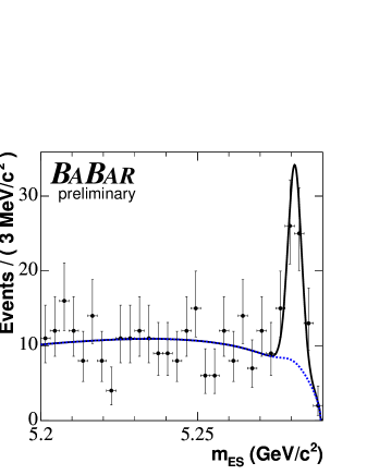
Figure 1: $B^{-}\rightarrow\tilde{D}^{0}K^{*-}$ $m_{\rm ES}$ distribution after all selection criteria are applied. The curves represent the fit projections for signal plus background (solid) and background (dotted).

4 THE $D^{0}\rightarrow K^{0}_{\scriptscriptstyle S}\pi^{-}\pi^{+}$ DECAY MODEL

The $D^{0}\rightarrow K^{0}_{\scriptscriptstyle S}\pi^{-}\pi^{+}$ decay amplitude ${\cal A}_{D}(m^{2}_{-},m^{2}_{+})$ is determined from an unbinned maximum-likelihood Dalitz fit to the Dalitz plot distribution of a high-purity (97%) sample of 81496 $D^{*+}\rightarrow D^{0}\pi^{+}$ decays reconstructed in 91.5 $\mbox{\,fb}^{-1}$ of data, shown in Fig. 2(a). We use two different models to describe ${\cal A}_{D}(m^{2}_{-},m^{2}_{+})$.

The first (Breit-Wigner) model is the same as used for our previously reported measurement of $\gamma$ on $B^{-}\rightarrow\tilde{D}^{(\ast)0}K^{-}$, $\tilde{D}^{0}\rightarrow K^{0}_{\scriptscriptstyle S}\pi^{-}\pi^{+}$ decays [5]. Here, the decay amplitude is expressed as a sum of two-body decay-matrix elements (subscript $r$) and a non-resonant (subscript NR) contribution,

$${\cal A}_{D}(m^{2}_{-},m^{2}_{+})=\mathchar 28934\relax_{r}a_{r}e^{i\phi_{r}}{\cal A}_{r}(m^{2}_{-},m^{2}_{+})+a_{\rm NR}e^{i\phi_{\rm NR}}~{},$$

where each term is parameterized with an amplitude $a_{r}$ and a phase $\phi_{r}$. The function ${\cal A}_{r}(m^{2}_{-},m^{2}_{+})$ is the Lorentz-invariant expression for the matrix element of a $D^{0}$ meson decaying into $K^{0}_{\scriptscriptstyle S}\pi^{-}\pi^{+}$ through an intermediate resonance $r$, parameterized as a function of position in the Dalitz plane. For $r=\rho(770)$ and $\rho(1450)$ we use the functional form suggested in Ref. [13], while the remaining resonances are parameterized by a spin-dependent relativistic Breit-Wigner distribution [2]. The model consists of 13 resonances leading to 16 two-body decay amplitudes and phases (see Table I in Ref. [5]), plus the non-resonant contribution, and accounts for efficiency variations across the Dalitz plane and the small background contribution (with uniform Dalitz shape). All the resonances considered in this model are well established except for the two scalar $\pi\pi$ resonances, $\sigma$ and $\sigma^{\prime}$, whose masses and widths are obtained from our sample. The $\sigma$ and $\sigma^{\prime}$ resonances are introduced in order to obtain a better fit to the data, but we consider in the evaluation of the systematic errors the possibility that they do not actually exist. We estimate the goodness of fit through a two-dimensional $\chi^{2}$ test and obtain $\chi^{2}=3824$ for $3054-32$ degrees of freedom. This model is the one used as nominal in this analysis.

The second ($\pi\pi$ S-wave K-matrix) model uses the K-matrix formalism [10, 11] to parameterize the S-wave component of the $\pi\pi$ system in $D^{0}\rightarrow K^{0}_{\scriptscriptstyle S}\pi^{-}\pi^{+}$. The K-matrix approach can be applied to the case of resonance production in multi-body decays when the two-body system in the final state is isolated, and the two particles do not interact simultaneously with the rest of the final state in the production process. In addition, it provides a direct way of imposing the unitarity constraint that is not guaranteed in the case of the Breit-Wigner model. Therefore, the K-matrix method is suited to the study of broad and overlapping resonances in multi-channel decays, solving the main limitation of the Breit-Wigner model to parameterize the $\pi\pi$ S-wave states in $D^{0}\rightarrow K^{0}_{\scriptscriptstyle S}\pi^{-}\pi^{+}$ [14], and avoiding the need to introduce the two $\sigma$ scalars.

The Dalitz amplitude ${\cal A}_{D}(m_{-}^{2},m_{+}^{2})$ is written in this case as a sum of two-body decay matrix elements for the spin-1, spin-2 and $K\pi$ spin-0 resonances (as in the Breit-Wigner model), and the $\pi\pi$ spin-0 piece denoted as $F_{1}$ is written in terms of the K-matrix. We have

$${\cal A}_{D}(m^{2}_{-},m^{2}_{+})=F_{1}(s)+\mathchar 28934\relax_{r\neq\pi\pi\,{\rm S-wave}}a_{r}e^{i\phi_{r}}{\cal A}_{r}(m^{2}_{-},m^{2}_{+})~{},$$ (3)

where $F_{1}(s)$ is the contribution of $\pi\pi$ S-wave states,

$$F_{1}(s)=\sum_{j}\left[I-iK(s)\rho(s)\right]^{-1}_{1j}P_{j}(s)~{}.$$ (4)

Here, $s$ is the squared mass of the $\pi\pi$ system $(m^{2}_{\pi^{+}\pi^{-}})$, $I$ is the identity matrix, $K$ is the matrix describing the $S$-wave scattering process, $\rho$ is the phase-space matrix, and $P$ is the initial production vector [11],

$$P_{j}(s)=\sum_{\alpha}\frac{\beta_{\alpha}g^{\alpha}_{j}}{m^{2}_{\alpha}-s}+f^{\rm prod}_{1j}\frac{1-s^{\rm scatt}_{0}}{s-s^{\rm scatt}_{0}}~{}.$$ (5)

The index $j$ represents the $j^{\rm th}$ channel ($1=\pi\pi$, $2=K\overline{K}$, $3=$multi-meson, $4=\eta\eta$, $5=\eta\eta^{\prime}$ [15]). The K-matrix parameters are obtained from Ref. [15] from a global fit of the available $\pi\pi$ scattering data from threshold up to $1900{\mathrm{\,Me\kern-1.00006ptV\!/}c^{2}}$. The K-matrix parameterization is

$$K_{ij}(s)=\left\{\sum_{\alpha}\frac{g^{\alpha}_{i}g^{\alpha}_{j}}{m^{2}_{\alpha}-s}+f^{\rm scatt}_{ij}\frac{1.0-s^{\rm scatt}_{0}}{s-s^{\rm scatt}_{0}}\right\}\frac{(1-s_{A0})}{(s-s_{A0})}(s-s_{A}m^{2}_{\pi}/2),$$ (6)

where $g^{\alpha}_{i}$ is the coupling constant of the K-matrix pole $m_{\alpha}$ to the $i^{\rm th}$ channel. The parameters $f^{\rm scatt}_{ij}$ and $s^{\rm scatt}_{0}$ describe the slowly-varying part of the K-matrix element. The Adler zero factor $(1-s_{A0})(s-s_{A}m^{2}_{\pi}/2)/(s-s_{A0})$ [16] suppresses false kinematical singularity at $s=0$ in the physical region near the $\pi\pi$ threshold [17]. Note that the production vector has the same poles as the K-matrix, otherwise the $F_{1}$ vector would vanish (diverge) at the K-matrix (P-vector) poles. The parameter values used in this analysis are listed in Table 1 [18]. The parameters $f^{\rm scatt}_{ij}$, for $i\neq 1$, are all set to zero since they are not related to the $\pi\pi$ scattering process.

Table 1: K-matrix parameters as obtained from Refs. [15, 18]. Pole masses ($m_{\alpha}$) and coupling constants ($g_{i}^{\alpha}$) are given in ${\mathrm{\,Ge\kern-1.00006ptV\!/}c^{2}}$, $s^{\rm scatt}_{0}$ and $s_{A0}$ are in ${\mathrm{\,Ge\kern-1.00006ptV^{2}\!/}c^{4}}$.

$m_{\alpha}$	$g_{\pi^{+}\pi^{-}}^{\alpha}$	$~{}g_{K\overline{K}}^{\alpha}$	$~{}g_{4\pi}^{\alpha}$	$~{}g_{\eta\eta}^{\alpha}$	$~{}g_{\eta\eta^{\prime}}^{\alpha}$
$0.651$	$0.229$	$-0.554$	$\phantom{-}0.000$	$-0.399$	$-0.346$
$1.204$	$0.941$	$\phantom{-}0.551$	$\phantom{-}0.000$	$\phantom{-}0.391$	$\phantom{-}0.315$
$1.558$	$0.369$	$\phantom{-}0.239$	$\phantom{-}0.556$	$\phantom{-}0.183$	$\phantom{-}0.187$
$1.210$	$0.337$	$\phantom{-}0.409$	$\phantom{-}0.857$	$\phantom{-}0.199$	$-0.010$
$1.822$	$0.182$	$-0.176$	$-0.797$	$-0.004$	$\phantom{-}0.224$
	$f^{\rm scatt}_{11}$	$~{}f^{\rm scatt}_{12}$	$~{}f^{\rm scatt}_{13}$	$~{}f^{\rm scatt}_{14}$	$~{}f^{\rm scatt}_{15}$
	$0.234$	$\phantom{-}0.150$	$-0.206$	$\phantom{-}0.328$	$\phantom{-}0.354$
	$~{}s^{\rm scatt}_{0}$	$~{}s_{A0}$	$~{}s_{A}$
	$-3.926$	$-0.15$	$\phantom{-}1$

The phase space matrix is diagonal, $\rho_{ij}(s)=\delta_{ij}\rho_{i}(s)$, where

$$\rho_{i}(s)=\sqrt{1-\frac{(m_{1i}+m_{2i})^{2}}{s}}~{},$$ (7)

with $m_{1i}$ ($m_{2i}$) denoting the mass of the first (second) final state particle of the $i^{th}$ channel. The normalization is such that $\rho_{i}\rightarrow 1$ as $s\rightarrow\infty$. We use an analytic continuation of the $\rho_{i}$ functions below threshold. The expression of the multi-meson state phase space is written as [15]

$$\rho_{3}(s) =\left\{\begin{array}[]{ll}\rho_{31}&s<1~{}\mathrm{\,Ge\kern-1.00006ptV}^{2}\\ \rho_{32}&s>1~{}\mathrm{\,Ge\kern-1.00006ptV}^{2}\end{array}\right\},$$ (10)

where

$$\rho_{31}(s) = \rho_{0}\int\int\frac{ds_{1}}{\pi}\frac{ds_{2}}{\pi}\frac{M^{2}\Gamma(s_{1})\Gamma(s_{2})\sqrt{(s+s_{1}-s_{2})^{2}-4ss_{1}}}{s[(M^{2}-s_{1})^{2}+M^{2}\Gamma^{2}(s_{1})]\,[(M^{2}-s_{2})^{2}+M^{2}\Gamma^{2}(s_{2})]},$$

$$\rho_{32}(s) = \frac{s-16m^{2}_{\pi}}{s}~{}.$$ (11)

Here $s_{1}$ and $s_{2}$ are the squared invariant mass of the two dipion systems, $M$ is the $\rho$ meson mass, and $\Gamma(s)$ is the energy-dependent width. The factor $\rho_{0}$ provides the continuity of $\rho_{3}(s)$ at $s=1~{}\mathrm{\,Ge\kern-1.00006ptV}^{2}$. Energy conservation in the dipion system must be satisfied when calculating the integral. This complicated expression reveals the fact that the $\rho$ meson has an intrinsic width. If one sets $\Gamma(s)=\delta(s)$, where $\delta$ is the Dirac $\delta$ function, the usual two-body phase space factor is obtained.

Table 2 summarizes the values of the P-vector free parameters $\beta_{\alpha}$ and $f^{\rm prod}_{11}$ (we are describing only $\pi\pi$ channel), together with the spin-1, spin-2, and $K\pi$ spin-0 amplitudes as in the Breit-Wigner model. The third and fifth poles are not included since they are far beyond our $\pi\pi$ kinematic range. Figures 2(b,c,d) show the fit projections overlaid with the data distributions. There is no overall improvement in the two-dimensional $\chi^{2}$ test compared to the Breit-Wigner model [5] since it is dominated by the P-wave components, which are identical between the two models. The total fit fraction is slightly changed from 1.24 to 1.16. Nevertheless, it should be emphasized that the main advantage of using a K-matrix parameterization rather than a sum of two-body amplitudes to describe the $\pi\pi$ S-wave is that it provides a more adequate description of the complex dynamics in the presence of overlapping and many channel resonances.

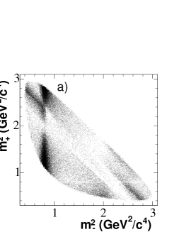
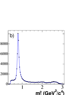
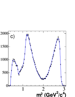
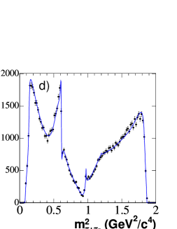
Figure 2: (a) The $D^{0}\rightarrow K^{0}_{\scriptscriptstyle S}\pi^{-}\pi^{+}$ Dalitz distribution from $D^{*+}\rightarrow D^{0}\pi^{+}$ events, and projections on (b) $m^{2}_{-}$, (c) $m^{2}_{+}$, and (d) $m^{2}_{\pi^{+}\pi^{-}}$. $\kern 1.99997pt\overline{\kern-1.99997ptD}{}^{0}\rightarrow K^{0}_{\scriptscriptstyle S}\pi^{+}\pi^{-}$ from $D^{*-}\rightarrow\kern 1.99997pt\overline{\kern-1.99997ptD}{}^{0}\pi^{-}$ events are also included. The curves are the $\pi\pi$ S-wave K-matrix model fit projections.

Table 2: Complex amplitudes $a_{r}e^{i\phi_{r}}$ and fit fractions of the different components ($K^{0}_{\scriptscriptstyle S}\pi^{-}$ and $K^{0}_{\scriptscriptstyle S}\pi^{+}$ resonances, and $\pi^{+}\pi^{-}$ poles) obtained from the fit of the $D^{0}\rightarrow K^{0}_{\scriptscriptstyle S}\pi^{-}\pi^{+}$ Dalitz distribution from $D^{*+}\rightarrow D^{0}\pi^{+}$ events. Errors are statistical only. Masses and widths of all resonances are taken from [2], while the pole masses and scattering data are from [15, 18]. The fit fraction is defined for the resonance terms ($\pi\pi$ S-wave term) as the integral of $a_{r}^{2}|{\cal A}_{r}(m^{2}_{-},m^{2}_{+})|^{2}$ ($|F_{1}(s)|^{2}$) over the Dalitz plane divided by the integral of $|{\cal A}_{D}(m^{2}_{-},m^{2}_{+})|^{2}$. The sum of fit fractions is $1.16$.

Component	$\mathop{\rm Re}\{a_{r}e^{i\phi_{r}}\}$	$\mathop{\rm Im}\{a_{r}e^{i\phi_{r}}\}$	Fit fraction (%)
$K^{*}(892)^{-}$	$-1.159\pm 0.022$	$1.361\pm 0.020$	$58.9$
$K^{*}_{0}(1430)^{-}$	$2.482\pm 0.075$	$-0.653\pm 0.073$	$9.1$
$K^{*}_{2}(1430)^{-}$	$0.852\pm 0.042$	$-0.729\pm 0.051$	$3.1$
$K^{*}(1410)^{-}$	$-0.402\pm 0.076$	$0.050\pm 0.072$	$0.2$
$K^{*}(1680)^{-}$	$-1.00\pm 0.29$	$1.69\pm 0.28$	$1.4$
$K^{*}(892)^{+}$	$0.133\pm 0.008$	$-0.132\pm 0.007$	$0.7$
$K^{*}_{0}(1430)^{+}$	$0.375\pm 0.060$	$-0.143\pm 0.066$	$0.2$
$K^{*}_{2}(1430)^{+}$	$0.088\pm 0.037$	$-0.057\pm 0.038$	$0.0$
$\rho(770)$	1 (fixed)	0 (fixed)	$22.3$
$\omega(782)$	$-0.0182\pm 0.0019$	$0.0367\pm 0.0014$	$0.6$
$f_{2}(1270)$	$0.787\pm 0.039$	$-0.397\pm 0.049$	$2.7$
$\rho(1450)$	$0.405\pm 0.079$	$-0.458\pm 0.116$	$0.3$
$\beta_{1}$	$-3.78\pm 0.13$	$1.23\pm 0.16$	$-$
$\beta_{2}$	$9.55\pm 0.20$	$3.43\pm 0.40$	$-$
$\beta_{4}$	$12.97\pm 0.67$	$1.27\pm 0.66$	$-$
$f_{11}^{\rm prod}$	$-10.22\pm 0.32$	$-6.35\pm 0.39$	$-$
sum of $\pi^{+}\pi^{-}$ S-wave			$16.2$

5 CP ANALYSIS

We perform an unbinned extended maximum-likelihood fit to the $B^{-}\rightarrow\tilde{D}^{0}K^{*-}$ sample to extract the $C\!P$-violating parameters $x_{s\mp}$, $y_{s\mp}$, and $r_{s}^{2}$ along with the signal and background yields. The $x_{s\pm}$ and $y_{s\pm}$ variables are more suitable fit parameters than $\kappa r_{s}$, $\delta_{s}$ and $\gamma$ because they are better behaved near the origin, especially in low-statistics samples. The fit uses $m_{\rm ES}$ and the same Fisher discriminant $\mathcal{F}$ as used in [5] to distinguish events from $B\kern 1.79993pt\overline{\kern-1.79993ptB}{}$ production and continuum background. The Fisher is a linear combination of four topological variables: $L_{0}=\sum_{i}p_{i}^{*}$, $L_{2}=\sum_{i}p_{i}^{*}|\cos\theta^{*}_{i}|^{2}$, and the absolute values of the cosine of the CM polar angles of the $B$ candidate momentum and thrust direction. Here, $p_{i}^{*}$ and $\theta_{i}^{*}$ are the CM momentum and the angle with respect to the $B$ candidate thrust axis of the remaining tracks and clusters in the event. The likelihood for candidate $j$ is obtained by summing the product of the event yield $N_{c}$, the probability density functions (PDF’s) for the kinematic and event shape variables ${\cal P}_{c}$, and the Dalitz distributions ${\cal P}_{c}^{\rm Dalitz}$, over the signal and background components $c$. The overall likelihood function is

$${\cal L}=\exp\left(-\sum_{c}N_{c}\right)\prod_{j}\sum_{c}N_{c}{\cal P}_{c}(\vec{\xi}_{j}){\cal P}^{\rm Dalitz}_{c}(\vec{\eta}_{j})~{},$$

where $\vec{\xi}_{j}=\{\mbox{$m_{\rm ES}$},\mbox{$\mathcal{F}$}\}_{j}$, $\vec{\eta}_{j}=(m_{-}^{2},m_{+}^{2})_{j}$, and ${\cal P}_{c}(\vec{\xi})={\cal P}_{c}(\mbox{$m_{\rm ES}$}){\cal P}_{c}(\mbox{$\mathcal{F}$})$. The components in the fit are signal, continuum background, and $B\kern 1.79993pt\overline{\kern-1.79993ptB}{}$ background. For signal events, ${\cal P}^{\rm Dalitz}_{c}(\vec{\eta})$ is given by $\Gamma_{\mp}(\vec{\eta})$ corrected by the efficiency variations, where $\Gamma_{\mp}(\vec{\eta})$ is given by Eq. (2). The $m_{\rm ES}$ ($\mathcal{F}$) distribution for signal events is described by a Gaussian (double-Gaussian) function distribution whose parameters are determined from a fit to the same $B^{-}\rightarrow D^{0}\pi^{-}$ high-statistics control sample as in our previous analysis [5].

5.1 Background composition

The event yields $N_{c}$ for signal, continuum, and $B\kern 1.79993pt\overline{\kern-1.79993ptB}{}$ components are, respectively, $42\pm 8$, $251\pm 24$, and $45\pm 21$, in agreement with our expectation from simulation and measured branching ratios. The dominant background contribution is from the random combination of a real or fake $D^{0}$ meson with a charged track and a $K^{0}_{\scriptscriptstyle S}$ in continuum events or other $B\kern 1.79993pt\overline{\kern-1.79993ptB}{}$ decays. The continuum background in the $m_{\rm ES}$ distribution is described by a threshold function [19] whose free parameter $\zeta$ is determined from the $B^{-}\rightarrow D^{0}\pi^{-}$ control sample. The Fisher PDF for continuum background is determined using $B^{-}\rightarrow D^{0}\pi^{-}$ events from the $m_{\rm ES}$ sideband region. The shape of the background $m_{\rm ES}$ distribution in generic $B\kern 1.79993pt\overline{\kern-1.79993ptB}{}$ decays is taken from simulation and uses a threshold function to describe the combinatorial component plus a Gaussian distribution to parameterize the peaking contribution arising from events with a misreconstructed pion and having a topology similar to that of signal events. The Gaussian component has a width of $3.8\pm 1.4$ ${\mathrm{\,Ge\kern-1.00006ptV\!/}c^{2}}$ and its fraction with respect to the total $B\kern 1.79993pt\overline{\kern-1.79993ptB}{}$ background is $0.13\pm 0.03$. The Fisher PDF and the mean of the $m_{\rm ES}$ Gaussian for $B\kern 1.79993pt\overline{\kern-1.79993ptB}{}$ events are assumed to be the same as that for the signal.

An important class of background events arises from continuum and $B\kern 1.79993pt\overline{\kern-1.79993ptB}{}$ background events where a real $D^{0}$ is produced back-to-back with a $K^{*}$ in the CM. Depending on the flavor-charge correlation this background can mimic either the $b\rightarrow c$ or the $b\rightarrow u$ signal component. In the likelihood function we take this effect into account with two parameters, the fraction $f_{D^{0}}$ of background events with a real $D^{0}$ and the parameter $R$, the fraction of background events with a real $D^{0}$ associated with an oppositely flavored kaon (same charge correlation as the $b\rightarrow u$ signal component). These fractions have been evaluated separately from continuum and generic $B\kern 1.79993pt\overline{\kern-1.79993ptB}{}$ simulated events, and are found to be $f_{D^{0}}^{q\overline{q}}=0.21\pm 0.02$, $f_{D^{0}}^{B\kern 1.25995pt\overline{\kern-1.25995ptB}{}}=0.18\pm 0.02$, $R^{q\overline{q}}=0.51\pm 0.06$ and $R^{B\kern 1.25995pt\overline{\kern-1.25995ptB}{}}=0.67\pm 0.06$. In addition, to check the reliability of these estimates, the fraction $f_{D^{0}}$ for all background (continuum and $B\kern 1.79993pt\overline{\kern-1.79993ptB}{}$) events has been evaluated from data using events satisfying $\mbox{$m_{\rm ES}$}<5.272$ ${\mathrm{\,Ge\kern-1.00006ptV\!/}c^{2}}$ after removing the requirement on the $D^{0}$ mass cut. The measured value of $0.20\pm 0.06$ is consistent with the continuum and $B\kern 1.79993pt\overline{\kern-1.79993ptB}{}$ fractions obtained from simulated events. The shapes of the Dalitz plot distributions are parameterized by a third-order polynomial in $(m_{-}^{2},m_{+}^{2})$ for the combinatorial component (fake $D^{0}$) and as signal $D^{0}$ or $\kern 1.99997pt\overline{\kern-1.99997ptD}{}^{0}$ shapes for real neutral $D$ mesons. The parameters of the polynomials are extracted from off-resonance data and sidebands for the continuum component, while we use the simulation for $B\kern 1.79993pt\overline{\kern-1.79993ptB}{}$.

A potentially dangerous background originates from signal $B^{-}\rightarrow\tilde{D}^{0}K^{*-}$ where the $\tilde{D}^{0}$ meson is combined with a random $K^{*}$ or pion from the other $B$ meson having the opposite charge. Using simulated events the fraction of these wrong sign signal events is found to be $(0.43\pm 0.05)$%, and therefore this contribution has been neglected.

5.2 $C\!P$ parameters

The Dalitz plot distributions for the $\tilde{D}^{0}\rightarrow K^{0}_{\scriptscriptstyle S}\pi^{-}\pi^{+}$ decay from $B^{-}\rightarrow\tilde{D}^{0}K^{*-}$ for events with $\mbox{$m_{\rm ES}$}>5.272$ ${\mathrm{\,Ge\kern-1.00006ptV\!/}c^{2}}$ are shown in Fig. 3. The distributions for $B^{-}$ and $B^{+}$ candidates are shown separately. The results for the $C\!P$-violating parameters $x_{s\pm}$ and $y_{s\pm}$ obtained by fitting those distributions are summarized in Table 3. From the same fit we obtain for $r_{s}^{2}$ the value $0.05\pm 0.11$ (statistical error only). The only relevant statistical correlations involving the $C\!P$ parameters are for the pairs $(x_{s-},y_{s-})$ and $(x_{s+},y_{s+})$, which amount to $-10.1\%$ and $2.2\%$, respectively. The statistical correlation of $r_{s}^{2}$ with $x_{s-}$, $y_{s-}$, $x_{s+}$, and $y_{s+}$ are $-22.6\%$, $3.7\%$, $-25.1\%$, and $22.0\%$, respectively. The Dalitz distribution projections on $m^{2}_{-}$, $m^{2}_{+}$ and $m^{2}_{\pi^{+}\pi^{-}}$ for events satisfying $\mbox{$m_{\rm ES}$}>5.272$ ${\mathrm{\,Ge\kern-1.00006ptV\!/}c^{2}}$ are compared to the projection of the fit in Fig. 4, separately for $B^{-}$ and $B^{+}$ events. Figure 5 shows the two-dimensional one- (dark) and two- (light) standard deviation regions (statistical only) in the $(x_{s},y_{s})$ plane, corresponding to 39.3% and 86.5% probability content, separately for $B^{-}\rightarrow\tilde{D}^{0}K^{*-}$ and $B^{+}\rightarrow\tilde{D}^{0}K^{*+}$. The separation $d$ between the $B^{-}$ and $B^{+}$ regions in these planes is proportional to the amount of direct $C\!P$ violation, $d=2\kappa r_{s}|\sin\gamma|$.

Table 3: $C\!P$-violating parameters $(x_{s\pm},y_{s\pm})$ obtained from the $C\!P$ fit to the $B^{-}\rightarrow\tilde{D}^{0}K^{*-}$ sample. The first error is statistical, the second is the experimental systematic uncertainty and the third reflects the Dalitz model uncertainty.

$C\!P$ parameter	Result
$x_{s-}\equiv\kappa r_{s}\cos(\delta_{s}-\gamma)$	$-0.20\pm 0.20\pm 0.11\pm 0.03$
$y_{s-}\equiv\kappa r_{s}\sin(\delta_{s}-\gamma)$	$\phantom{-}0.26\pm 0.30\pm 0.16\pm 0.03$
$x_{s+}\equiv\kappa r_{s}\cos(\delta_{s}+\gamma)$	$-0.07\pm 0.23\pm 0.13\pm 0.03$
$y_{s+}\equiv\kappa r_{s}\sin(\delta_{s}+\gamma)$	$-0.01\pm 0.32\pm 0.18\pm 0.05$

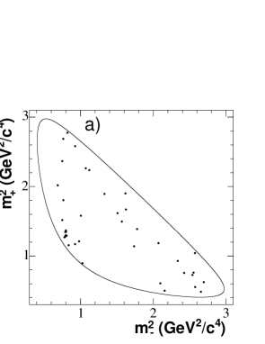
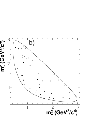
Figure 3: The $\tilde{D}^{0}\rightarrow K^{0}_{\scriptscriptstyle S}\pi^{-}\pi^{+}$ Dalitz distributions from (a) $B^{-}\rightarrow\tilde{D}^{0}K^{*-}$ and (b) $B^{+}\rightarrow\tilde{D}^{0}K^{*+}$ events with $\mbox{$m_{\rm ES}$}>5.272$ ${\mathrm{\,Ge\kern-1.00006ptV\!/}c^{2}}$.

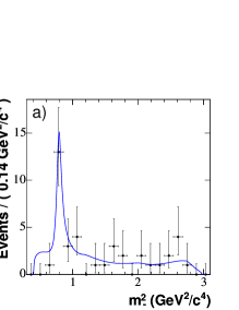
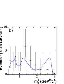
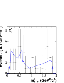
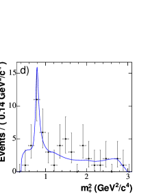
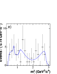
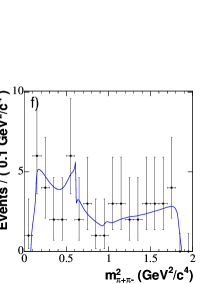
Figure 4: Projections of the Dalitz distributions on $m^{2}_{-}$, $m^{2}_{+}$ and $m^{2}_{\pi^{+}\pi^{-}}$ from a)b)c) $B^{-}\rightarrow\tilde{D}^{0}K^{*-}$ and d)e)f) $B^{+}\rightarrow\tilde{D}^{0}K^{*+}$ events with $\mbox{$m_{\rm ES}$}>5.272$ ${\mathrm{\,Ge\kern-1.00006ptV\!/}c^{2}}$. The projections of the fit result are superimposed.

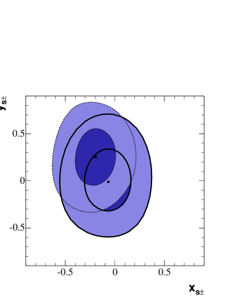
Figure 5: Two-dimensional one- (dark) and two- (light) standard deviation regions (statistical only) in the $(x_{s},y_{s})$ plane, corresponding to 39.3% and 86.5% probability content, separately for $B^{-}\rightarrow\tilde{D}^{0}K^{*-}$ (thick and solid) and $B^{+}\rightarrow\tilde{D}^{0}K^{*+}$ (thin and dotted). The confidence regions for $B^{+}$ are superimposed over those for $B^{-}$.

5.3 Experimental systematic errors

Table 4 summarizes the break down of the experimental systematic uncertainties. These include the errors on the $m_{\rm ES}$ and $\mathcal{F}$ PDF parameters for signal and background, the uncertainties in the knowledge of the Dalitz distribution of background events, the efficiency variations across the Dalitz plane, and the uncertainty in the fraction of events with a real $D^{0}$ produced in a back-to-back configuration with a negatively-charged kaon. Less significant systematic uncertainties originate from the imprecise knowledge of the fraction of real $D^{0}$’s, the invariant mass resolution (negligible), tracking efficiency, and the statistical errors in the Dalitz amplitudes and phases from the fit to the tagged $D^{0}$ sample. We quote as systematic uncertainty, for each effect, the maximum of the difference between the bias and square root of the quadratic difference of the statistical error between the nominal fit result and the one corresponding to the effect under consideration. These systematic uncertainties will be reduced with a larger data and simulated samples and are not expected to limit the eventual sensitivity of the analysis.

Table 4: Summary of the non-negligible contributions to the systematic error on the $C\!P$ parameters $x_{s\pm}$ and $y_{s\pm}$.

Source	$x_{s-}$	$y_{s-}$	$x_{s+}$	$y_{s+}$
$m_{\rm ES}$, $\mathcal{F}$ shapes	0.08	0.12	0.10	0.12
Background Dalitz shape	0.04	0.09	0.04	0.09
Efficiency in the Dalitz plot	0.06	0.04	0.07	0.09
Right sign $\tilde{D}^{0}$ fractions ($R^{q\overline{q}}$, $R^{B\kern 1.25995pt\overline{\kern-1.25995ptB}{}}$)	0.03	0.04	0.03	0.05
Real $\tilde{D}^{0}$ fractions ($f_{D^{0}}^{q\overline{q}}$, $f_{D^{0}}^{B\kern 1.25995pt\overline{\kern-1.25995ptB}{}}$)	0.03	0.03	0.03	0.04
Tracking efficiency	0.01	0.01	0.01	0.01
Dalitz amplitudes and phases	0.01	0.01	0.01	0.01
Total experimental	0.11	0.16	0.13	0.18
Dalitz model (Breit-Wigner model without $\sigma$ scalars)	0.03	0.03	0.03	0.05
Dalitz model ($\pi\pi$ S-wave K-matrix model)	0.01	0.01	0.01	0.01

5.4 $\tilde{D}^{0}\rightarrow K^{0}_{\scriptscriptstyle S}\pi^{-}\pi^{+}$ Dalitz model systematic uncertainty

The largest single contribution to the systematic uncertainties in the $C\!P$ parameters comes from the choice of the Dalitz model used to describe the $D^{0}\rightarrow K^{0}_{\scriptscriptstyle S}\pi^{-}\pi^{+}$ decay amplitude ${\cal A}_{D}$. We use the same procedure as in our previous measurement [5] to evaluate this uncertainty. We first generate large samples of pseudo-experiments using the nominal (Breit-Wigner) model. Since the effect on the $C\!P$ parameters depends on their generated values, for each pseudo-experiment we randomly generate the truth values of the Cartesian $C\!P$ parameters according to their measured central values and statistical errors. We then compare experiment by experiment the values of the $x_{s\pm}$ and $y_{s\pm}$ obtained from fits using the nominal model and a set of alternative models. We find that models resulting by removing different combinations of higher $K^{*}$ and $\rho$ resonances (with low fit fractions), or changing the functional form of the resonance shapes, has little effect on the total $\chi^{2}$ of the fit, or on the values of the $C\!P$ parameters (at most $1^{\circ}$ for $\gamma$ and $0.002$ for $\kappa r_{s}$). As an extreme we consider a model without the $\sigma_{1}$ and/or $\sigma_{2}$ scalar resonances, or the CLEO Breit-Wigner model [9]. Fits to these models result in a significantly larger $\chi^{2}$ than that of the nominal model, but the effect on the $C\!P$ parameters are still small, as indicated in Table 4. These uncertainties translate to $\kappa r_{s}$, $\gamma$ and $\delta_{s}$ as 0.05, $9^{\circ}$, and $11^{\circ}$, respectively . For $B^{-}\rightarrow\tilde{D}^{(\ast)0}K^{-}$ decays, the same procedure to propagate the uncertainties on $r^{(\ast)}_{B}$, $\gamma$, and $\delta^{(\ast)}_{B}$ gives $0.027(0.027)$, $11^{\circ}$, and $14^{\circ}(13^{\circ})$, respectively.

As an additional cross-check of the fact that models without the $\sigma$ scalars are in fact an extreme case, we repeated the above procedure using as alternative model the $\pi\pi$ S-wave K-matrix model described in Sec. 4 instead of the CLEO Breit-Wigner model (the latter used to quote the Dalitz model systematic uncertainty, as described before). The effect on the Cartesian $C\!P$ parameters is more than three times smaller, as shown in Table 4. These uncertainties translate to $\kappa r_{s}$, $\gamma$ and $\delta_{s}$ as 0.015, $3^{\circ}$, and $2^{\circ}$, respectively. For $B^{-}\rightarrow\tilde{D}^{(\ast)0}K^{-}$ decays, the scaling of the effect on the Cartesian $C\!P$ parameters is similar to $B^{-}\rightarrow DK^{*-}$. In terms of $r^{(\ast)}_{B}$, $\gamma$, and $\delta^{(\ast)}_{B}$ the variation is $0.004(0.003)$, $2^{\circ}$, and $2^{\circ}(2^{\circ})$, respectively.

6 INTERPRETATION AND RESULTS

A frequentist (Neyman) analysis [2] has been adopted to interpret the constraints on ${\bf z}_{\pm}\equiv(x_{s\pm},y_{s\pm})$ in terms of ${\bf p}\equiv(\kappa r_{s},\delta_{s},\gamma)$. We construct an analytical parameterization of the four-dimensional probability density function ${\cal P}$ of ${\bf z}_{\pm}$ as a function of ${\bf p}$,

$$\frac{d^{4}{\cal P}}{d^{2}{\bf z}_{+}d^{2}{\bf z}_{-}}({\bf z}_{+},{\bf z}_{-}|{\bf p}) = \frac{d^{2}{\cal P}}{d^{2}{\bf z}_{+}}({\bf z}_{+}|{\bf p})\frac{d^{2}{\cal P}}{d^{2}{\bf z}_{-}}({\bf z}_{-}|{\bf p})~{},$$ (12)

where

$$\frac{d^{2}{\cal P}}{d^{2}{\bf z}_{\pm}}({\bf z}_{\pm}|{\bf p}) = G_{2}\left[{\bf z}_{\pm};\kappa r_{s}\cos(\delta_{s}\pm\gamma),\kappa r_{s}\sin(\delta_{s}\pm\gamma),\sigma_{x_{s\pm}},\sigma_{y_{s\pm}},\rho_{s\pm}\right]$$ (13)

is a two-dimensional Gaussian distribution [20]. Here, $\rho_{s\pm}$ represents the correlation between $x_{s\pm}$ and $y_{s\pm}$. For a given ${\bf p}$, the three-dimensional confidence level is estimated as ${\cal C}({\bf p})=1-\alpha({\bf p})$, where $\alpha({\bf p})$ is calculated by integrating Eq. (12) over a domain defined by all points in the four-dimensional fit parameter space closer (larger PDF) to ${\bf p}$ than the fitted data values,

$$\frac{d^{4}{\cal P}}{d^{2}{\bf z}_{+}d^{2}{\bf z}_{-}}({\bf z}_{+},{\bf z}_{-}|{\bf p})\geq\frac{d^{4}{\cal P}}{d^{2}{\bf z}_{+}d^{2}{\bf z}_{-}}({\bf z}_{+}^{\rm data},{\bf z}_{-}^{\rm data}|{\bf p})~{}.$$ (14)

The one (two) standard deviation region of the $C\!P$ parameters is defined as the set of ${\bf p}$ values (constructed from a large number of pseudo-experiments) for which $\alpha({\bf p})$ is smaller than 19.88% (73.85%). Figure 6 shows the constraints in the $\kappa r_{s}-\gamma$ plane as obtained by projecting the three-dimensional confidence regions, including statistical and experimental systematic uncertainties.

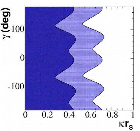
Figure 6: Two-dimensional projection onto the $\kappa r_{s}-\gamma$ plane of the three-dimensional one- (dark) and two- (light) standard deviation regions, including statistical and experimental systematic uncertainties, for $B^{-}\rightarrow\tilde{D}^{0}K^{*-}$.

$B^{-}\rightarrow\tilde{D}^{0}K^{*-}$ events can be used in combination with $B^{-}\rightarrow\tilde{D}^{(\ast)0}K^{-}$ [5] to improve the overall constraints on $\gamma$. The procedure used to combine the three $B$ decay channels is identical to the one described above, but with increased number of dimensions. In this case, the dimension of the fit parameter space is twelve, ${\bf z_{\pm}}\equiv(x_{\pm}^{(\ast)},y_{\pm}^{(\ast)},x_{s\pm},y_{s\pm})$. The $C\!P$ parameter space has instead seven dimensions, ${\bf p}\equiv(r^{(\ast)}_{B},\delta^{(\ast)}_{B},\kappa r_{s},\delta_{s},\gamma)$. The one (two) standard deviation region of the $C\!P$ parameters is defined as the set of ${\bf p}$ values for which $\alpha({\bf p})$ is larger than 0.52% (22.02%). Figure 7 shows the two-dimensional projections onto the $r_{B}-\gamma$, $r^{\ast}_{B}-\gamma$, and $\kappa r_{s}-\gamma$ planes, including statistical and experimental systematic uncertainties. The figures show that this Dalitz analysis has a two-fold ambiguity. The combination if the three signal modes yields $\gamma=\left(67\pm 28\pm 13\pm 11\right)^{\circ}$, where the first error is statistical, the second is the experimental systematic uncertainty and the third reflects the Dalitz model uncertainty. Of the two possible solutions we choose the one with $0<\gamma<180^{\circ}$. The contribution to the Dalitz model uncertainty due to the description of the $\pi\pi$ S-wave in $D^{0}\rightarrow K^{0}_{\scriptscriptstyle S}\pi^{-}\pi^{+}$ is $3^{\circ}$. From this combination, $\kappa r_{s}$ is constrained to be $<0.50~{}(0.75)$ at one (two) standard deviation level. It is worth noting that the value of $\kappa r_{s}$ depends on the selected phase space region of $B^{-}\rightarrow\tilde{D}^{0}(K^{0}_{\scriptscriptstyle S}\pi^{-})$ events without introducing any bias on the extraction of $\gamma$.

The constraint on $\gamma$ is consistent with that reported by the Belle Collaboration [6, 7]. However, the statistical error turns out to be larger than that of Belle because our data favors smaller values of $r^{(\ast)}_{B}$ and $\kappa r_{s}$. Simulation studies confirm that the difference in statistical errors is consistent with the scaling expected from the different actual values.

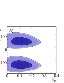
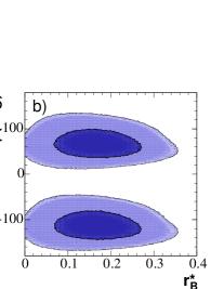
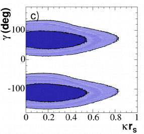
Figure 7: Two-dimensional projections onto the (a) $r_{B}-\gamma$, (b) $r^{\ast}_{B}-\gamma$, and (c) $\kappa r_{s}-\gamma$ planes of the seven-dimensional one- (dark) and two- (light) standard deviation regions, for the combination of $B^{-}\rightarrow\tilde{D}^{(\ast)0}K^{-}$ and $B^{-}\rightarrow\tilde{D}^{0}K^{*-}$ modes.

7 ACKNOWLEDGMENTS

We are grateful for the extraordinary contributions of our PEP-II colleagues in achieving the excellent luminosity and machine conditions that have made this work possible. The success of this project also relies critically on the expertise and dedication of the computing organizations that support BABAR. The collaborating institutions wish to thank SLAC for its support and the kind hospitality extended to them. This work is supported by the US Department of Energy and National Science Foundation, the Natural Sciences and Engineering Research Council (Canada), Institute of High Energy Physics (China), the Commissariat à l’Energie Atomique and Institut National de Physique Nucléaire et de Physique des Particules (France), the Bundesministerium für Bildung und Forschung and Deutsche Forschungsgemeinschaft (Germany), the Istituto Nazionale di Fisica Nucleare (Italy), the Foundation for Fundamental Research on Matter (The Netherlands), the Research Council of Norway, the Ministry of Science and Technology of the Russian Federation, and the Particle Physics and Astronomy Research Council (United Kingdom). Individuals have received support from CONACyT (Mexico), the A. P. Sloan Foundation, the Research Corporation, and the Alexander von Humboldt Foundation.

References

- [1] N. Cabibbo, Phys. Rev. Lett. 10, 531 (1963); M. Kobayashi and T. Maskawa, Prog. Theor. Phys. 49, 652 (1973).
- [2] Particle Data Group, S. Eidelman et al., Phys. Lett. B 592, 1 (2004).
- [3] M. Gronau and D. London, Phys. Lett. B 253, 483 (1991); M. Gronau and D. Wyler, Phys. Lett. B 265, 172 (1991); D. Atwood, I. Dunietz and A. Soni, Phys. Rev. Lett. 78, 3257 (1997).
- [4] A. Giri, Yu. Grossman, A. Soffer and J. Zupan, Phys. Rev. D 68, 054018 (2003).
- [5] BABAR Collaboration, B. Aubert et al., hep-ex/0504039, Accepted by Phys. Rev. Lett. .
- [6] Belle Collaboration, A. Poluektov et al., Phys. Rev. D 70, 072003 (2004); K. Abe et al., hep-ex/0411049.
- [7] Belle Collaboration, K. Abe et al., hep-ex/0504013.
- [8] M. Gronau, Phys. Lett. B557, 198 (2003).
- [9] CLEO Collaboration, S. Kopp et al., Phys. Rev. D 63, 092001 (2001); CLEO Collaboration, H. Muramatsu et al., Phys. Rev. Lett. 89, 251802 (2002); Erratum-ibid: 90 059901 (2003).
- [10] E. P. Wigner, Phys. Rev. 70 (1946) 15; S. U. Chung et al., Ann. Physik 4 (1995) 404.
- [11] I. J. R. Aitchison, Nucl. Phys. A189, 417 (1972).
- [12] BABAR Collaboration, B. Aubert et al., Nucl. Instrum. Methods A479, 1-116 (2002).
- [13] G.J. Gounaris and J.J. Sakurai, Phys. Rev. Lett. 21, 244, (1968).
- [14] Review on Scalar Mesons in Ref. [2].
- [15] V. V. Anisovich and A. V. Sarantev, Eur. Phys. Jour. A 16, 229 (2003).
- [16] FOCUS Collaboration, J. M. Link et al., Phys. Lett. B 585, 200 (2004). One should note that there is a misprint of the factor in the Adler zero expression.
- [17] S. L. Adler, Phys. Rev. 137, B1022 (1965).
- [18] V. V. Anisovich and A. V. Sarantev, private communication.
- [19] where and the parameter is determined from a fit. ARGUS Collaboration, H. Albrecht et al., Z. Phys. C 48, 543 (1990).
- [20] As given by Eq. (31.28) in Ref. [2].