Inclusive jet cross sections and
dijet correlations in photoproduction
at HERA
Abstract
Inclusive jet cross sections in photoproduction for events containing a meson have been measured with the ZEUS detector at HERA using an integrated luminosity of . The events were required to have a virtuality of the incoming photon, , of less than 1 GeV2, and a photon-proton centre-of-mass energy in the range . The measurements are compared with next-to-leading-order (NLO) QCD calculations. Good agreement is found with the NLO calculations over most of the measured kinematic region. Requiring a second jet in the event allowed a more detailed comparison with QCD calculations. The measured dijet cross sections are also compared to Monte Carlo (MC) models which incorporate leading-order matrix elements followed by parton showers and hadronisation. The NLO QCD predictions are in general agreement with the data although differences have been isolated to regions where contributions from higher orders are expected to be significant. The MC models give a better description than the NLO predictions of the shape of the measured cross sections.
DESY–05–132
The ZEUS Collaboration
S. Chekanov,
M. Derrick,
S. Magill,
S. Miglioranzi1,
B. Musgrave,
J. Repond,
R. Yoshida
Argonne National Laboratory, Argonne, Illinois 60439-4815, USA n
M.C.K. Mattingly
Andrews University, Berrien Springs, Michigan 49104-0380, USA
N. Pavel, A.G. Yagües Molina
Institut für Physik der Humboldt-Universität zu Berlin,
Berlin, Germany
P. Antonioli,
G. Bari,
M. Basile,
L. Bellagamba,
D. Boscherini,
A. Bruni,
G. Bruni,
G. Cara Romeo,
L. Cifarelli,
F. Cindolo,
A. Contin,
M. Corradi,
S. De Pasquale,
P. Giusti,
G. Iacobucci,
A. Margotti,
A. Montanari,
R. Nania,
F. Palmonari,
A. Pesci,
A. Polini,
L. Rinaldi,
G. Sartorelli,
A. Zichichi
University and INFN Bologna, Bologna, Italy e
G. Aghuzumtsyan,
D. Bartsch,
I. Brock,
S. Goers,
H. Hartmann,
E. Hilger,
P. Irrgang2,
H.-P. Jakob,
O.M. Kind,
U. Meyer,
E. Paul3,
J. Rautenberg,
R. Renner,
M. Wang,
M. Wlasenko
Physikalisches Institut der Universität Bonn,
Bonn, Germany b
D.S. Bailey4,
N.H. Brook,
J.E. Cole,
G.P. Heath,
T. Namsoo,
S. Robins
H.H. Wills Physics Laboratory, University of Bristol,
Bristol, United Kingdom m
M. Capua,
S. Fazio,
A. Mastroberardino,
M. Schioppa,
G. Susinno,
E. Tassi
Calabria University,
Physics Department and INFN, Cosenza, Italy e
J.Y. Kim,
K.J. Ma5
Chonnam National University, Kwangju, South Korea g
M. Helbich,
Y. Ning,
Z. Ren,
W.B. Schmidke,
F. Sciulli
Nevis Laboratories, Columbia University, Irvington on Hudson,
New York 10027 o
J. Chwastowski,
A. Eskreys,
J. Figiel,
A. Galas,
M. Gil,
K. Olkiewicz,
P. Stopa,
D. Szuba,
L. Zawiejski
The Henryk Niewodniczanski Institute of Nuclear Physics, Polish Academy of Sciences, Cracow,
Poland i
L. Adamczyk,
T. Bołd,
I. Grabowska-Bołd,
D. Kisielewska,
J. Łukasik,
M. Przybycień,
L. Suszycki,
J. Szuba6
Faculty of Physics and Applied Computer Science,
AGH-University of Science and Technology, Cracow, Poland p
A. Kotański7,
W. Słomiński
Department of Physics, Jagellonian University, Cracow, Poland
V. Adler,
U. Behrens,
I. Bloch,
K. Borras,
G. Drews,
J. Fourletova,
A. Geiser,
D. Gladkov,
P. Göttlicher8,
O. Gutsche,
T. Haas,
W. Hain,
C. Horn,
B. Kahle,
U. Kötz,
H. Kowalski,
G. Kramberger,
H. Lim,
B. Löhr,
R. Mankel,
I.-A. Melzer-Pellmann,
C.N. Nguyen,
D. Notz,
A.E. Nuncio-Quiroz,
A. Raval,
R. Santamarta,
U. Schneekloth,
H. Stadie,
U. Stösslein,
G. Wolf,
C. Youngman,
W. Zeuner
Deutsches Elektronen-Synchrotron DESY, Hamburg, Germany
S. Schlenstedt
Deutsches Elektronen-Synchrotron DESY, Zeuthen, Germany
G. Barbagli,
E. Gallo,
C. Genta,
P. G. Pelfer
University and INFN, Florence, Italy e
A. Bamberger,
A. Benen,
F. Karstens,
D. Dobur,
N.N. Vlasov9
Fakultät für Physik der Universität Freiburg i.Br.,
Freiburg i.Br., Germany b
P.J. Bussey,
A.T. Doyle,
W. Dunne,
J. Ferrando,
J.H. McKenzie,
D.H. Saxon,
I.O. Skillicorn
Department of Physics and Astronomy, University of Glasgow,
Glasgow, United Kingdom m
I. Gialas10
Department of Engineering in Management and Finance, Univ. of
Aegean, Greece
T. Carli11,
T. Gosau,
U. Holm,
N. Krumnack12,
E. Lohrmann,
M. Milite,
H. Salehi,
P. Schleper,
T. Schörner-Sadenius,
S. Stonjek13,
K. Wichmann,
K. Wick,
A. Ziegler,
Ar. Ziegler
Hamburg University, Institute of Exp. Physics, Hamburg,
Germany b
C. Collins-Tooth14,
C. Foudas,
C. Fry,
R. Gonçalo15,
K.R. Long,
A.D. Tapper
Imperial College London, High Energy Nuclear Physics Group,
London, United Kingdom m
M. Kataoka16,
K. Nagano,
K. Tokushuku17,
S. Yamada,
Y. Yamazaki
Institute of Particle and Nuclear Studies, KEK,
Tsukuba, Japan f
A.N. Barakbaev,
E.G. Boos,
N.S. Pokrovskiy,
B.O. Zhautykov
Institute of Physics and Technology of Ministry of Education and
Science of Kazakhstan, Almaty, Kazakhstan
D. Son
Kyungpook National University, Center for High Energy Physics, Daegu,
South Korea g
J. de Favereau,
K. Piotrzkowski
Institut de Physique Nucléaire, Université Catholique de
Louvain, Louvain-la-Neuve, Belgium q
F. Barreiro,
C. Glasman18,
M. Jimenez,
L. Labarga,
J. del Peso,
J. Terrón,
M. Zambrana
Departamento de Física Teórica, Universidad Autónoma
de Madrid, Madrid, Spain l
F. Corriveau,
C. Liu,
M. Plamondon,
A. Robichaud-Veronneau,
R. Walsh,
C. Zhou
Department of Physics, McGill University,
Montréal, Québec, Canada H3A 2T8 a
T. Tsurugai
Meiji Gakuin University, Faculty of General Education,
Yokohama, Japan f
A. Antonov,
B.A. Dolgoshein,
I. Rubinsky,
V. Sosnovtsev,
A. Stifutkin,
S. Suchkov
Moscow Engineering Physics Institute, Moscow, Russia j
R.K. Dementiev,
P.F. Ermolov,
L.K. Gladilin,
I.I. Katkov,
L.A. Khein,
I.A. Korzhavina,
V.A. Kuzmin,
B.B. Levchenko,
O.Yu. Lukina,
A.S. Proskuryakov,
L.M. Shcheglova,
D.S. Zotkin,
S.A. Zotkin
Moscow State University, Institute of Nuclear Physics,
Moscow, Russia k
I. Abt,
C. Büttner,
A. Caldwell,
X. Liu,
J. Sutiak
Max-Planck-Institut für Physik, München, Germany
N. Coppola,
G. Grigorescu,
A. Keramidas,
E. Koffeman,
P. Kooijman,
E. Maddox,
H. Tiecke,
M. Vázquez,
L. Wiggers
NIKHEF and University of Amsterdam, Amsterdam, Netherlands h
N. Brümmer,
B. Bylsma,
L.S. Durkin,
A. Lee,
T.Y. Ling
Physics Department, Ohio State University,
Columbus, Ohio 43210 n
P.D. Allfrey,
M.A. Bell, A.M. Cooper-Sarkar,
A. Cottrell,
R.C.E. Devenish,
B. Foster,
C. Gwenlan19,
T. Kohno,
K. Korcsak-Gorzo,
S. Patel,
V. Roberfroid20,
P.B. Straub,
R. Walczak
Department of Physics, University of Oxford,
Oxford United Kingdom m
P. Bellan,
A. Bertolin, R. Brugnera,
R. Carlin,
R. Ciesielski,
F. Dal Corso,
S. Dusini,
A. Garfagnini,
S. Limentani,
A. Longhin,
L. Stanco,
M. Turcato
Dipartimento di Fisica dell’ Università and INFN,
Padova, Italy e
E.A. Heaphy,
F. Metlica,
B.Y. Oh,
J.J. Whitmore21
Department of Physics, Pennsylvania State University,
University Park, Pennsylvania 16802 o
Y. Iga
Polytechnic University, Sagamihara, Japan f
G. D’Agostini,
G. Marini,
A. Nigro
Dipartimento di Fisica, Università ’La Sapienza’ and INFN,
Rome, Italy
J.C. Hart
Rutherford Appleton Laboratory, Chilton, Didcot, Oxon,
United Kingdom m
H. Abramowicz22,
A. Gabareen,
S. Kananov,
A. Kreisel,
A. Levy
Raymond and Beverly Sackler Faculty of Exact Sciences,
School of Physics, Tel-Aviv University, Tel-Aviv, Israel d
M. Kuze
Department of Physics, Tokyo Institute of Technology,
Tokyo, Japan f
S. Kagawa,
T. Tawara
Department of Physics, University of Tokyo,
Tokyo, Japan f
R. Hamatsu,
H. Kaji,
S. Kitamura23,
K. Matsuzawa,
O. Ota,
Y.D. Ri
Tokyo Metropolitan University, Department of Physics,
Tokyo, Japan f
M. Costa,
M.I. Ferrero,
V. Monaco,
R. Sacchi,
A. Solano
Università di Torino and INFN, Torino, Italy e
M. Arneodo,
M. Ruspa
Università del Piemonte Orientale, Novara, and INFN, Torino,
Italy e
S. Fourletov,
J.F. Martin
Department of Physics, University of Toronto, Toronto, Ontario,
Canada M5S 1A7 a
J.M. Butterworth24,
R. Hall-Wilton,
T.W. Jones,
J.H. Loizides25,
M.R. Sutton4,
C. Targett-Adams,
M. Wing
Physics and Astronomy Department, University College London,
London, United Kingdom m
J. Ciborowski26,
G. Grzelak,
P. Kulinski,
P. Łużniak27,
J. Malka27,
R.J. Nowak,
J.M. Pawlak,
J. Sztuk28,
T. Tymieniecka,
A. Ukleja,
J. Ukleja29,
A.F. Żarnecki
Warsaw University, Institute of Experimental Physics,
Warsaw, Poland
M. Adamus,
P. Plucinski
Institute for Nuclear Studies, Warsaw, Poland
Y. Eisenberg,
D. Hochman,
U. Karshon,
M.S. Lightwood
Department of Particle Physics, Weizmann Institute, Rehovot,
Israel c
E. Brownson,
T. Danielson,
A. Everett,
D. Kçira,
S. Lammers,
L. Li,
D.D. Reeder,
M. Rosin,
P. Ryan,
A.A. Savin,
W.H. Smith
Department of Physics, University of Wisconsin, Madison,
Wisconsin 53706, USA n
S. Dhawan
Department of Physics, Yale University, New Haven, Connecticut
06520-8121, USA n
S. Bhadra,
C.D. Catterall,
Y. Cui,
G. Hartner,
S. Menary,
U. Noor,
M. Soares,
J. Standage,
J. Whyte
Department of Physics, York University, Ontario, Canada M3J
1P3 a
1 also affiliated with University College London, UK
2 now at Siemens VDO/Sensorik, Weissensberg
3 retired
4 PPARC Advanced fellow
5 supported by a scholarship of the World Laboratory
Björn Wiik Research Project
6 partly supported by Polish Ministry of Scientific Research and Information
Technology, grant no.2P03B 12625
7 supported by the Polish State Committee for Scientific Research, grant no.
2 P03B 09322
8 now at DESY group FEB, Hamburg, Germany
9 partly supported by Moscow State University, Russia
10 also affiliated with DESY
11 now at CERN, Geneva, Switzerland
12 now at Baylor University, USA
13 now at University of Oxford, UK
14 now at the Department of Physics and Astronomy, University of Glasgow, UK
15 now at Royal Holloway University of London, UK
16 also at Nara Women’s University, Nara, Japan
17 also at University of Tokyo, Japan
18 Ramón y Cajal Fellow
19 PPARC Postdoctoral Research Fellow
20 EU Marie Curie Fellow
21 on leave of absence at The National Science Foundation, Arlington, VA, USA
22 also at Max Planck Institute, Munich, Germany, Alexander von Humboldt
Research Award
23 Department of Radiological Science
24 also at University of Hamburg, Germany, Alexander von Humboldt Fellow
25 partially funded by DESY
26 also at Łódź University, Poland
27 Łódź University, Poland
28 Łódź University, Poland, supported by the KBN grant 2P03B12925
29 supported by the KBN grant 2P03B12725
| a | supported by the Natural Sciences and Engineering Research Council of Canada (NSERC) |
|---|---|
| b | supported by the German Federal Ministry for Education and Research (BMBF), under contract numbers HZ1GUA 2, HZ1GUB 0, HZ1PDA 5, HZ1VFA 5 |
| c | supported in part by the MINERVA Gesellschaft für Forschung GmbH, the Israel Science Foundation (grant no. 293/02-11.2), the U.S.-Israel Binational Science Foundation and the Benozyio Center for High Energy Physics |
| d | supported by the German-Israeli Foundation and the Israel Science Foundation |
| e | supported by the Italian National Institute for Nuclear Physics (INFN) |
| f | supported by the Japanese Ministry of Education, Culture, Sports, Science and Technology (MEXT) and its grants for Scientific Research |
| g | supported by the Korean Ministry of Education and Korea Science and Engineering Foundation |
| h | supported by the Netherlands Foundation for Research on Matter (FOM) |
| i | supported by the Polish State Committee for Scientific Research, grant no. 620/E-77/SPB/DESY/P-03/DZ 117/2003-2005 and grant no. 1P03B07427/2004-2006 |
| j | partially supported by the German Federal Ministry for Education and Research (BMBF) |
| k | supported by RF Presidential grant N 1685.2003.2 for the leading scientific schools and by the Russian Ministry of Education and Science through its grant for Scientific Research on High Energy Physics |
| l | supported by the Spanish Ministry of Education and Science through funds provided by CICYT |
| m | supported by the Particle Physics and Astronomy Research Council, UK |
| n | supported by the US Department of Energy |
| o | supported by the US National Science Foundation |
| p | supported by the Polish Ministry of Scientific Research and Information Technology, grant no. 112/E-356/SPUB/DESY/P-03/DZ 116/2003-2005 and 1 P03B 065 27 |
| q | supported by FNRS and its associated funds (IISN and FRIA) and by an Inter-University Attraction Poles Programme subsidised by the Belgian Federal Science Policy Office |
:
1 Introduction
Charm and/or jet production in collisions should be accurately calculable in perturbative Quantum Chromodynamics (pQCD) since the mass of the heavy quark, , and the transverse energy of the jet, , provide hard scales. In photoproduction, where a quasi-real photon, emitted from the incoming lepton, collides with a parton from the incoming proton, such events can be classified into two types of process in leading-order (LO) QCD. In direct processes, the photon couples as a point-like object in the hard scatter. In resolved processes, the photon acts as a source of incoming partons with only a fraction of its momentum participating in the hard scatter.
Measurements of the photoproduction cross section [1] as functions of the transverse momentum, , and the pseudorapidity, , show that the predictions from next-to-leading-order (NLO) QCD are too low for 3 GeV and . Part of this deficit may be due to hadronisation effects. The predictions for jet production accompanied by a meson should have smaller uncertainties from these hadronisation effects. Furthermore jets can be measured in a wider pseudorapidity range than mesons due to the larger acceptance of the calorimeter compared to the central tracker.
A dijet sample of photoproduction can also be used to study higher-order QCD topologies [1, 2]. In the present paper, previously unmeasured correlations between the two jets of highest transverse energy, namely the difference in azimuthal angle, , and the squared transverse momentum of the dijet system, , which are particularly sensitive to higher-order topologies, are presented. For the LO process, the two jets are produced back-to-back with and . Large deviations from these values may come from higher-order QCD effects. The accuracy of the theoretical description of these effects is tested.
Calculations performed to NLO in QCD are available with two different treatments for charm. In the fixed-order, or “massive”, scheme [3, *np:b454:3], , and are the only active flavours in the structure functions of the proton and photon; charm and beauty are produced only in the hard scatter. This scheme is expected to work well in regions where the transverse momentum of the outgoing quark is of the order of the quark mass. At higher transverse momenta, the resummed or “massless” scheme [5, *zfp:c76:689, 7] should be applicable. In this scheme, charm and beauty are regarded as active flavours (massless partons) in the structure functions of the proton and photon and are fragmented from massless partons into massive hadrons after the hard process.
In this paper, photoproduction of charm is studied by tagging a meson and reconstructing at least one jet in the final state. The measurement is performed in the following kinematic region: photon virtuality, ; photon-proton centre-of-mass energy, ; ; ; jet transverse energy, ; and jet pseudorapidity, . Differential cross sections as a function of and have been measured. Jets are divided into two categories: jets of the first category are associated with the meson (-tagged jet), while jets of the second category are not matched to a meson (untagged jet). The inclusive, -tagged and untagged jet cross sections are compared to the massive NLO QCD predictions. A comparison to the massless calculation is only available for the untagged jet cross sections [8].
A sub-sample having at least two jets with and is used to measure the correlations between the two highest jets: the fraction of the photon momentum participating in dijet production, [9]; ; ; and the dijet invariant mass, . Differential dijet cross sections as a function of these variables have been measured for the direct-enriched () and resolved-enriched () kinematic regions and compared to massive NLO QCD predictions and Monte Carlo (MC) models.
2 Experimental set-up
The analysis was performed with data taken from 1998 to 2000, when HERA collided electrons or positrons111Hereafter, both electrons and positrons are referred to as electrons, unless explicitly stated otherwise. with energy 27.5 GeV with protons of energy 920 GeV resulting in a centre-of-mass energy of 318 GeV. The results are based on an integrated luminosity of of collision data taken by the ZEUS detector. A detailed description of the ZEUS detector can be found elsewhere [10]. A brief outline of the components that are most relevant for this analysis is given below.
Charged particles are tracked in the central tracking detector (CTD) [11, *npps:b32:181, *nim:a338:254], which operates in a magnetic field of provided by a thin superconducting coil. The CTD consists of 72 cylindrical drift chamber layers, organised in 9 superlayers covering the polar-angle222The ZEUS coordinate system is a right-handed Cartesian system, with the axis pointing in the proton beam direction, referred to as the “forward direction”, and the axis pointing left towards the center of HERA. The coordinate origin is at the nominal interaction point. region . The transverse-momentum resolution for full-length tracks is , with in GeV.
The high-resolution uranium–scintillator calorimeter (CAL) [14, *nim:a309:101, *nim:a321:356, *nim:a336:23] consists of three parts: the forward (FCAL), the barrel (BCAL) and the rear (RCAL) calorimeters. Each part is subdivided transversely into towers and longitudinally into one electromagnetic section (EMC) and either one (in RCAL) or two (in BCAL and FCAL) hadronic sections (HAC). The smallest subdivision of the calorimeter is called a cell. The CAL energy resolutions, as measured under test-beam conditions, are for electrons and for hadrons ( in GeV).
The luminosity was measured from the rate of the bremsstrahlung process , where the photon was measured in a lead–scintillator calorimeter [18, *zfp:c63:391, *acpp:b32:2025] placed in the HERA tunnel at .
3 Event reconstruction and selection
A three-level trigger system was used to select events online [10, 21]. At the first- and second-level triggers, general characteristics of photoproduction events were required and background due to beam-gas interactions rejected. At the third level, a candidate was reconstructed.
In the offline analysis, the hadronic final state and jets were reconstructed using a combination of track and calorimeter information that optimises the resolution of reconstructed kinematic variables [22]. The selected tracks and calorimeter clusters are referred to as Energy Flow Objects (EFOs). To select photoproduction events, the following criteria were used:
-
•
the event vertex was required to be within of the nominal vertex position in the longitudinal direction;
-
•
deep inelastic scattering (DIS) events with a scattered electron candidate in the CAL were removed [23]. To keep the events where a pion was misidentified as a scattered electron, events where 0.7 were retained; and are the energy and polar angle, respectively, of the scattered electron candidate;
-
•
the requirement GeV was imposed, where and is the estimator of the inelasticity, , measured from the EFOs according to the Jacquet-Blondel method [24]. Here, was corrected, using MC simulation, for the energy losses of EFOs in inactive material in front of the CAL. The upper cut removed DIS events where the scattered electron was not identified and which, therefore, have a value of close to 1. The lower cut removed proton beam-gas events which have a low value of .
The cuts on and restricted the range of the virtuality of the exchanged photon to less than about 1 GeV2, with a median value of about 3 10-4 .
3.1 reconstruction
The mesons were identified using the decay channel with the subsequent decay and the corresponding antiparticle decay, where refers to a low-momentum (“slow”) pion accompanying the .
Charged tracks measured by the CTD and assigned to the primary event vertex were selected. The transverse momentum was required to be greater than 0.12 GeV. Each track was required to reach at least the third superlayer of the CTD. These restrictions ensured that the track acceptance and momentum resolution were high. Tracks in the CTD with opposite charges and transverse momenta were combined in pairs to form candidates. The tracks were alternately assigned the masses of a kaon and a pion and the invariant mass of the pair, , was evaluated. Each additional track, with charge opposite to that of the kaon track, was assigned the pion mass and combined with the -meson candidate to form a candidate.
The signal regions for the reconstructed masses, and , were GeV and GeV, respectively. For background determination, candidates with wrong-sign combinations, in which both tracks forming the candidates have the same charge and the third track has the opposite charge, were also retained. The same kinematic restrictions were applied as for those candidates with correct-charge combinations. The normalisation factor of the wrong-charge sample was determined as the ratio of events with correct-charge combinations to wrong-charge combinations in the region GeV.
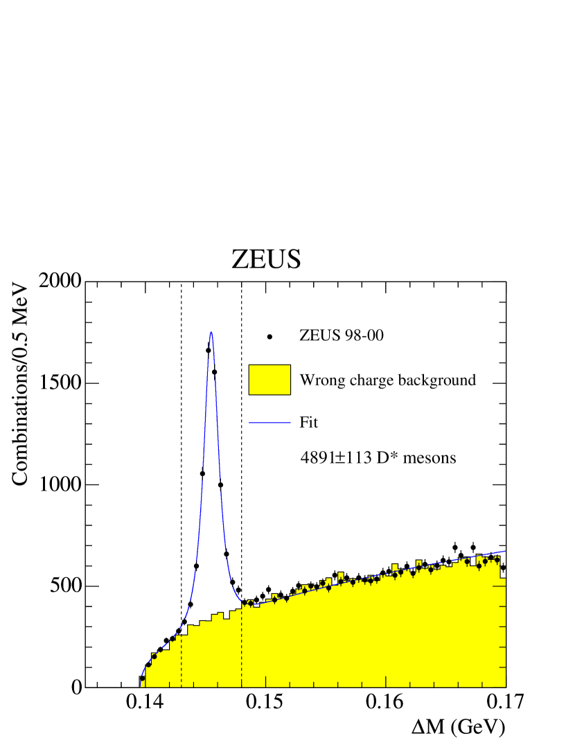
The kinematic region for candidates was GeV and . Figure 1 shows for the selection of a meson with a jet (see Section 3.2). The fit to the distribution has the form
where , are free parameters and is the pion mass. The “modified” Gaussian described both data and MC distributions well. The fit gives a peak at (stat.) MeV to be compared to the PDG value of MeV [25]. The difference is due to systematic effects which are too small to be relevant for this analysis. The fitted width of MeV is consistent with the experimental resolution.
The number of mesons was determined from candidates reconstructed in both signal regions and after the subtraction of the background estimated from the wrong-charge sample; this gave mesons. This procedure was used throughout the paper with the number of mesons obtained from the fit used as a systematic check.
3.2 Jet reconstruction
Jets were reconstructed using EFOs as input to the the cluster algorithm [26] in its longitudinally invariant inclusive mode [27]. The transverse energy of the jet was corrected for energy losses in inactive material in front of the CAL, where the correction factors were determined in bins of and from MC simulation. These corrections were between 5% and 12%.
For the inclusive jet cross sections, jets with and were selected, and events containing at least one such jet were used for further analysis. For the dijet analysis, events were required to have at least two jets with and , while the highest jet was required in addition to satisfy . The asymmetric jet transverse-energy cut assures that the NLO calculation is not infrared sensitive [28]. After the dijet selection, mesons remained.
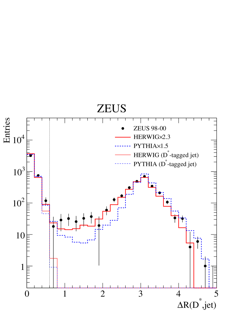
Cross sections are given separately for -tagged and untagged jets. -tagged jets are defined as jets in which a (in the kinematic region defined in Section 3.1) was clustered into the jet at the hadron level by the algorithm. All the other jets are called untagged jets. These two classes of jets can be distinguished experimentally by cutting on the distance between the and the jet, where and are the azimuthal angles of the meson and jet, respectively. Figure 2 shows the distance of the to all jets in the event for data and MC. The peak at is due to -tagged jets as indicated by the distribution for -tagged jets for the MC hadron-level predictions also shown in Fig. 2. The broad peak at is due to the untagged jets. A cut at was used to distinguish experimentally tagged and untagged jets. For the inclusive jet sample, 83% of mesons were matched to a jet, and for the dijet sub-sample 94% of mesons were matched to a jet.
4 Monte Carlo models
The MC programmes Herwig 6.301 [29, 30] and Pythia 6.156 [31], which implement LO matrix elements followed by parton showers and hadronisation, were used to model the final state. The Herwig and Pythia generators differ in the details of the implementation of the leading-logarithmic parton-shower models. They also use different hadronisation models: Herwig uses the cluster [32] model and Pythia uses the Lund string [33] model. Direct and resolved events were generated separately and in proportion to the cross sections predicted by the MC programme. The relative fraction of charm and beauty events was also generated in proportion to the cross sections predicted by the MC programme. Events were generated using CTEQ5L [34] and GRV-G LO parton density functions (PDF) for the proton and the photon, respectively. The -quark and -quark masses were set to and , respectively.
The MC programmes were used both to compare with the dijet cross sections, which are particularly sensitive to the parton-shower models and for calculation of the acceptance and effects of detector response (see Section 6). For all generated events, the ZEUS detector response was simulated in detail using a programme based on Geant 3.13 [35].
5 NLO QCD calculations
There are two NLO QCD calculations available to calculate jet cross sections in charm photoproduction: the massive calculation by Frixione et al. (FMNR) [3, *np:b454:3] and the massless calculation by Heinrich and Kniehl [8].
5.1 Massive calculation
In the massive calculation, the PDF sets used were CTEQ5M1 [34] for the proton and AFG-HO [36] for the photon. The renormalisation scale, , and factorisation scale, , were set to , where is the average squared transverse momentum of the two charm quarks and . The fragmentation of the charm quark into a meson was described by rescaling the -quark momentum using the Peterson fragmentation function [37] with which is taken from an NLO fit to ARGUS data [38]. The fraction of charm quarks hadronising into a meson was set to 0.235 [39]. The algorithm was applied to the outgoing partons in the final state of the NLO programme.
The dependence of the NLO prediction on different photon PDFs, , and was evaluated by repeating the calculation using different sets of parameters. The upper (lower) bound of the NLO QCD prediction was estimated by setting and ( and ).
An NLO prediction of production for beauty is not available so this contribution was estimated using a combination of the hadron cross section at NLO and decays in Pythia. The distributions of the two stable hadrons produced in the Pythia MC programme were reweighted to the distribution in the NLO calculation. In the NLO calculation, the -quark mass, , was set to 4.75 GeV, and [40]. The branching was set to the value measured by the OPAL Collaboration [41]. The upper (lower) bound of the NLO QCD prediction was estimated by setting and ( and ). The contribution from beauty production for the inclusive jet distribution, as predicted by NLO+Pythia, is about 2% at low and increases to 8% at high . For each cross section, this beauty contribution and its uncertainty were added linearly to the corresponding massive prediction from charm quarks.
5.2 Massless calculation
In the massless calculation, AFG04 [42] for the photon PDF and MRST03 [43, *epj:c23:73] for the proton PDF were used. The number of flavours was set to five. The fragmentation function and fraction of beauty and charm hadronising into a meson are derived [7, 8] from a fit to data from LEP; the function is assumed to be applicable to HERA as it is derived using the factorisation theorem in QCD. The central prediction uses , where . The fragmentation factorisation [8] scale, , and were set to .
The uncertainty was estimated by changing the scales to and for the upper bound, and and for the lower bound. The photon PDF, GRV-HO, was used, and the uncertainty was found to be less than half that from the variation in scale [8]. The difference between MRST01 and MRST03 proton PDFs was found to be negligible for the distributions considered. The size of the beauty contribution was estimated by suppressing the final-state fragmentation of a quark to a meson. This reduces the cross-section prediction by about 3% at low and 15% at high . Due to theoretical limitations, the predictions for the massless scheme can only be calculated for the untagged-jet distributions.
5.3 Hadronisation correction
As the NLO calculations produce final-state partons, the effects of hadronisation were considered when comparing the predictions with the data. The NLO QCD jet predictions were corrected using a bin-by-bin procedure according to , where is the cross section for parton jets in the final state of the NLO calculation. The hadronisation correction factor was defined as the ratio of the jet cross sections after and before the hadronisation process, . Here, parton-level cross sections were obtained using partons after the initial- and final-state showering of the MC simulations described in Section 4. Distributions at the parton level in the MC programmes were checked to be similar to those calculated using the NLO programme, assuring the validity of using a bin-by-bin correction. The value of was taken as the mean of the ratios obtained using the Herwig and Pythia predictions. The uncertainty on this value was estimated as half the difference between the values obtained using the two models. These uncertainties were added in quadrature to the other uncertainties of the NLO calculations. The values of applied to the NLO predictions are given in Tables 1–11.
6 Data correction and systematic uncertainties
The data were corrected, using the MC models described in Section 4, for the detector acceptance and the selection efficiencies to obtain differential cross sections for the process . The definition of the cross section includes events with a containing primary quarks or those from -quark decays. The data were initially compared to the MC simulation in shape and found generally to agree well for all the kinematic quantities. Since Herwig gives a better overall description of the data than Pythia, it was chosen as the primary MC model to correct the data. The cross section for a given observable was determined using
where is either the number of jets for the inclusive jet cross sections or the number of mesons for the dijet cross sections in a bin of size . The acceptance, , takes into account migrations and efficiencies for that bin, and is the integrated luminosity. The product, , of the appropriate branching ratios for the and was set to [25].
The systematic uncertainties of the measured cross sections were determined by changing the selection cuts or the analysis procedure in turn and repeating the extraction of the cross sections. The uncertainties are described in more detail elsewhere [45]. The following systematic studies have been carried out (the resulting uncertainty on the total cross section is given in parentheses):
-
•
varying the values of the selection cuts by the experimental resolutions in the corresponding quantity ();
-
•
varying the efficiencies of the CAL first-level trigger ();
-
•
the acceptance was recalculated by re-weighting the prediction from the Herwig MC simulation in to reproduce the distribution of this variable in the data (%);
-
•
an additional contribution to the uncertainty from the modelling of the hadronisation process was estimated by using Pythia instead of Herwig (%);
-
•
the effect of the uncertainty of the beauty cross section on the acceptance correction was taken into account by increasing the beauty contribution by a factor two (%);
-
•
varying the procedure to extract the signal (%);
-
•
varying by the jet energy scale in the CAL (%).
All systematic uncertainties were added in quadrature to obtain the total systematic uncertainty, except for the jet energy-scale uncertainty, as this has a large correlation between bins, and is shown separately in all figures. In most bins of the differential cross sections, the total systematic uncertainty is comparable to the statistical errors. In addition, an overall normalisation uncertainty of from the luminosity determination is included in neither the figures nor the tables.
7 Inclusive jet cross sections
Inclusive jet cross sections with a in the final state have been measured as a function of and in the following kinematic region:
-
•
and ;
-
•
and ;
-
•
and ;
-
•
a -jet match is required only where explicitly stated.
At the hadron level, the meson is used as input into the jet finder therefore allowing a -tagged jet to be identified unambiguously.
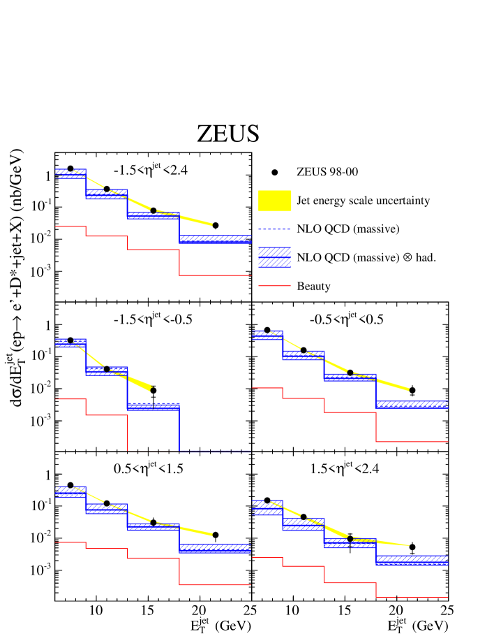
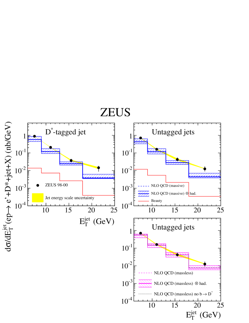
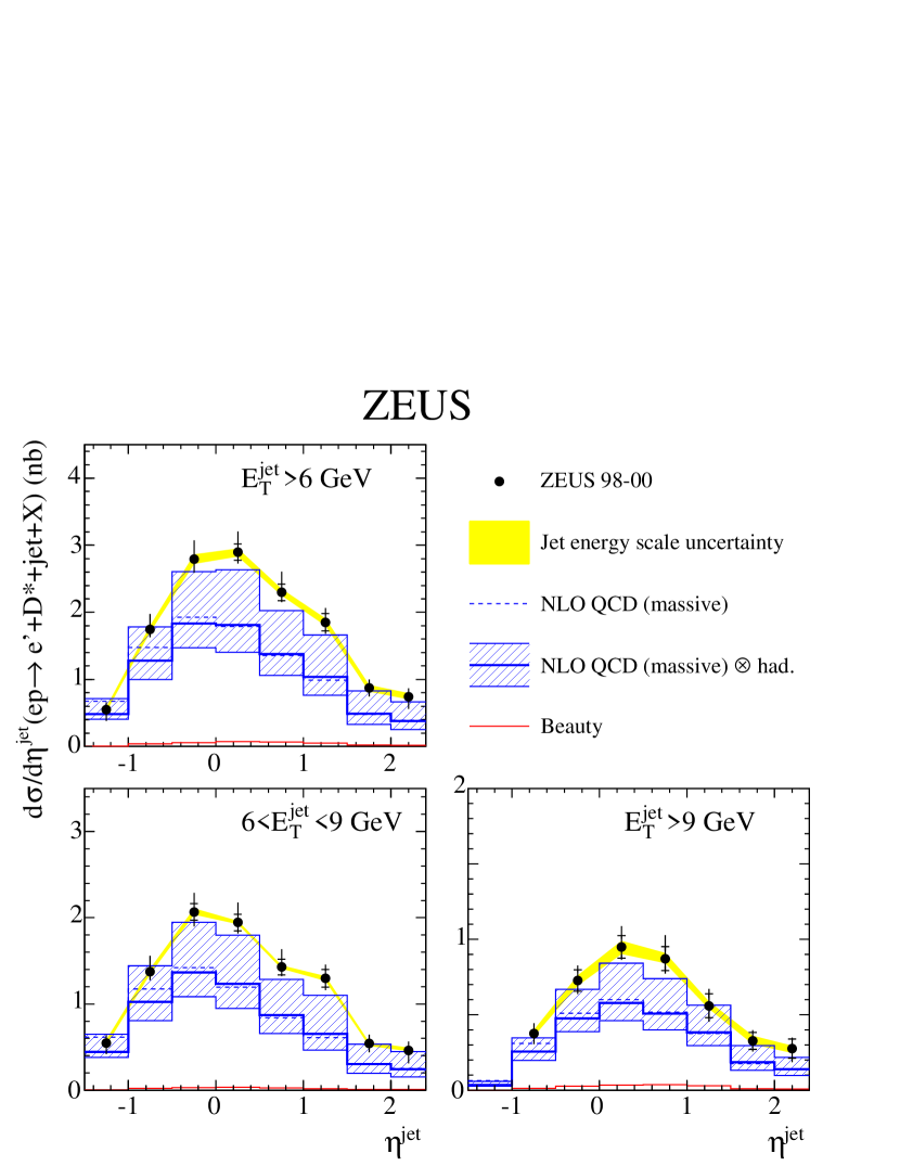
The cross-sections in bins of are shown in Fig. 3 and given in Table 1 for all jets and in Fig. 4 and Table 3 for the whole range for -tagged and untagged jets. The distributions tend to fall less steeply with increasing . The cross sections in different regions of are shown in Fig. 5 and given in Table 2 for all jets and in Fig. 6 and Tables LABEL:tbl:inclusive_eta_dstar and LABEL:tbl:inclusive_eta_other for -tagged and untagged jets. Due to the requirement , the -tagged jet is centred around and falls off rapidly at large . The advantage of reconstructing jets is observed in the untagged-jet distribution where a significant cross section is measured up to 2.4. This is due to the larger acceptance of the CAL compared to the CTD.
The massive calculation is compared to all measured cross sections whereas the massless calculation is compared only to the untagged-jet distributions. The normalisation of the data for all distributions is well described by the upper limit of both NLO QCD predictions. The shape of the data is well described by the NLO QCD predictions. The inclusion of hadronisation corrections which shift the distributions towards forward improves the description of the data. Some difference in shape is observed for the upper bound of the massless prediction compared to the untagged-jet distributions for 9 GeV (see Fig. 6).
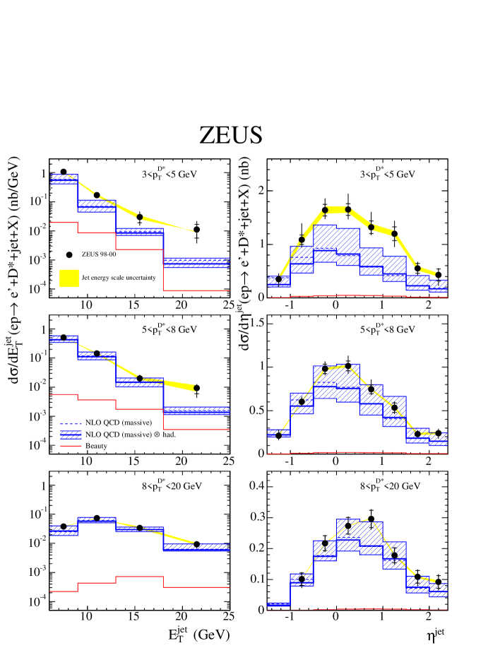
Measurements of and in bins of are given in Tables 5 and 6 and shown in Fig. 7 compared to the massive NLO prediction. The NLO prediction gives a poor description of the normalisation of the data at lowest . However, the normalisation of the NLO prediction agrees with the data in the two regions of higher . In all regions, the shape of the data is reasonably well described by the NLO prediction. Similar conclusions on the normalisation were seen for inclusive measurements [1]. However, the difference in shape observed as a function of in the inclusive measurement is not seen here as a function of . The -quark contribution is largest in the region of low .
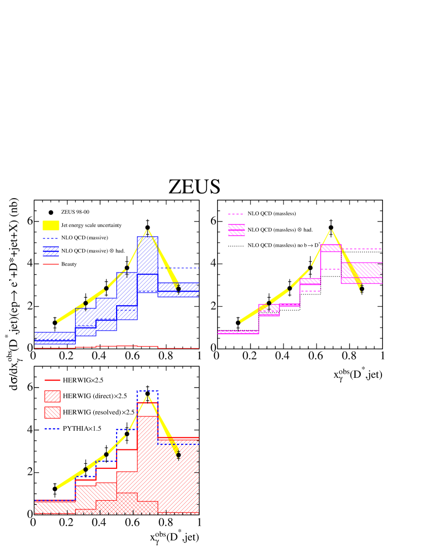
In order to be sensitive to higher-order effects, and to distinguish between direct-enriched and resolved-enriched regions, the variable was constructed [8], in an analogous way to the ‘traditional’ [9]. Using the meson and the untagged jet of highest , the quantity is given by:
| (1) |
This variable has the advantage of being calculable in the massless scheme. In addition it takes advantage of increased statistics by requiring only one jet of high . In Fig. 8 the measured cross-section , given in Table 7, is compared to both the massless and massive predictions. The upper bound of the massive prediction gives a good description of the data; the description of the massless prediction is somewhat worse. The Herwig MC model gives a poor description whilst Pythia gives a reasonable description of the shape of the data distribution. Both MC programmes underestimate the normalisation of the data.
8 Dijet cross sections
Dijet correlations are particularly sensitive to higher-order effects and therefore suitable to test the limitations of fixed-order perturbative QCD calculations. Events containing a meson were required to have at least two jets with , and . The , , and requirements were the same as for the inclusive jet cross section.
The dijet variables measured were reconstructed from the two highest jets as:
| (2) |
| (3) |
| (4) |
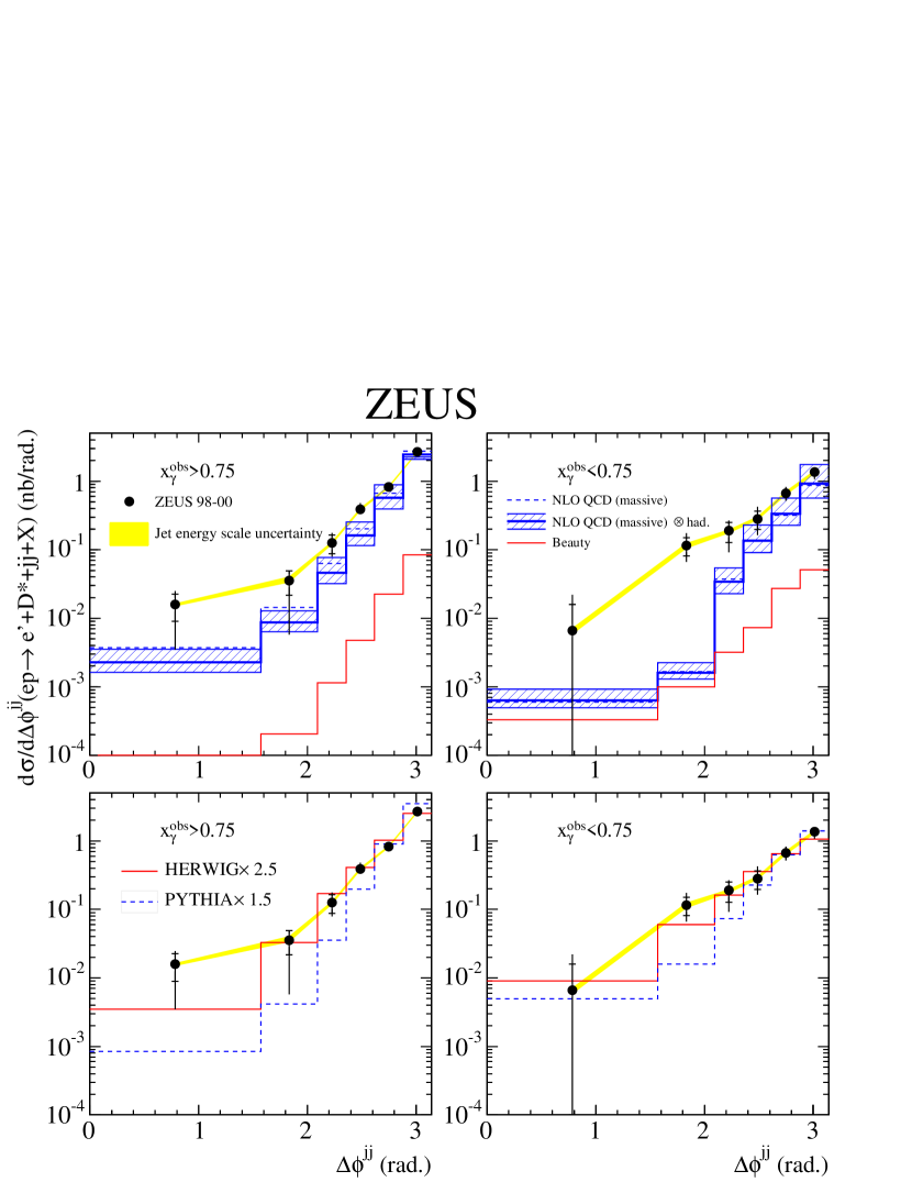
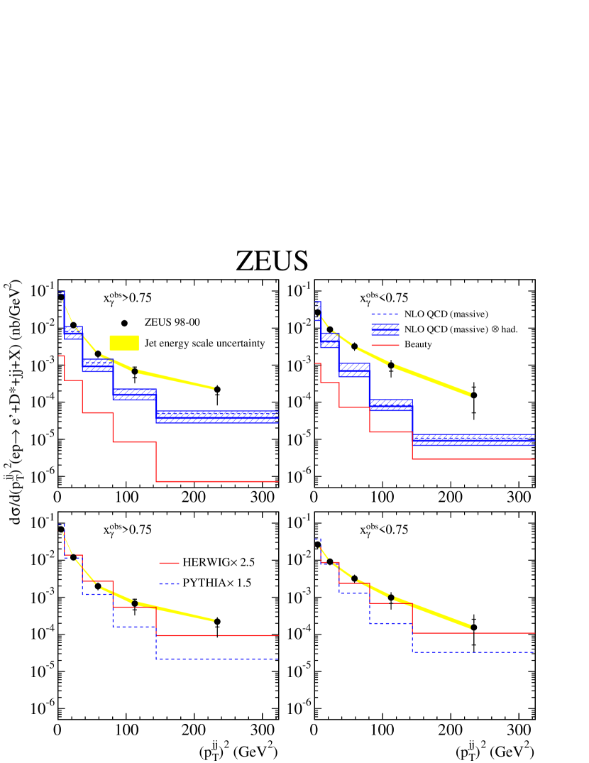
| (5) |
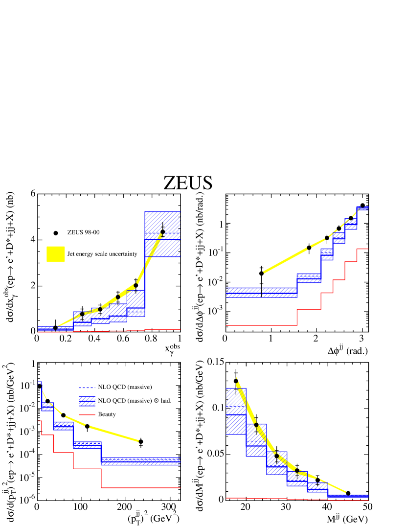
Table 8 gives, and Fig. 9a shows, the dijet cross section as a function of , which is reasonably well described by the massive calculation. In Tables 9-11 and Figs. 9b-d, the cross sections as a function of , and are also shown. For there is agreement between data and the NLO prediction at large angular separation, but at smaller values the NLO prediction underestimates the data. This is correlated with the agreement and disagreement at low and high values, respectively. The distribution in dijet invariant mass is described well by the upper limit of the NLO prediction, as was the case for the inclusive jet cross sections in Section 7.
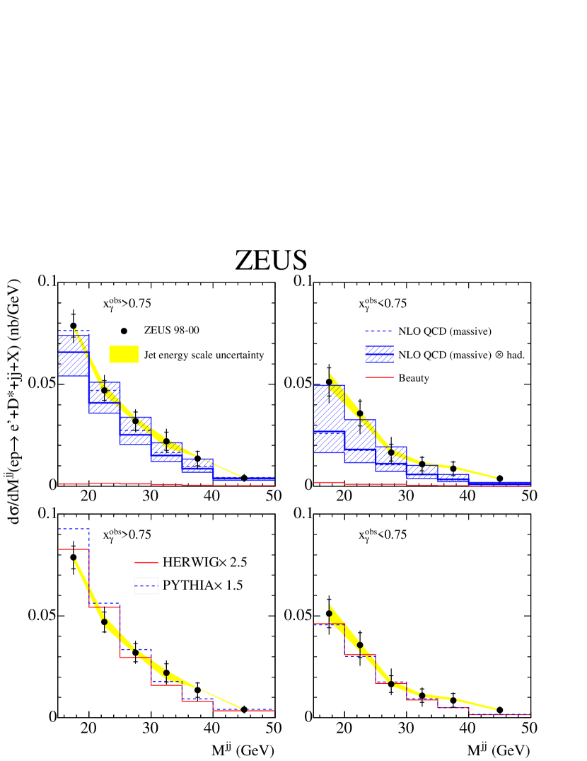
Cross sections as a function of , and are shown in Figs. 10–12 and given in Tables 9-11 separately for direct-enriched () and resolved-enriched () samples. The data are compared to massive NLO QCD predictions and expectations from MC models.
The cross-section in Fig. 10 is described well by the NLO prediction and both MC models, Herwig and Pythia, for both regions in .
The cross-sections (see Fig. 11) and (see Fig. 12) are reasonably well reproduced by the NLO prediction for although the data exhibit a somewhat harder distribution. For , the data exhibit a harder spectrum than for . The NLO prediction of the cross section for has a significantly softer distribution compared to the data, both as a function of and . The low- region is more sensitive to higher-order topologies not present in the massive NLO calculation. The predictions from the Pythia MC reproduce neither the shape nor the normalisation of the data for low and high . However, the predictions from the Herwig MC give an excellent description of the shapes of all distributions, although the normalisation is underestimated by a factor of 2.5. The fact that a MC programme incorporating parton showers can successfully describe the data whereas the NLO QCD prediction cannot indicates that the QCD calculation requires higher orders. Matching of parton showers with NLO calculations such as in the MC@NLO programme [46, *jhep:0308:007], which is not currently available for the processes studied here, should improve the description of the data.
9 Conclusions
Differential inclusive jet cross sections for events containing a meson have been measured with the ZEUS detector in the kinematic region , , , , and . The measurements are compared to NLO QCD predictions in the massive and massless schemes. With the addition of hadronisation corrections, the upper limit of both theoretical predictions show similar trends and reasonable agreement with all measured cross sections. Dijet correlation cross-sections and are well described by the massive NLO QCD prediction, although again the data tends to agree better with the upper bound of the NLO calculation. In contrast, the cross-sections and show a large deviation from the massive NLO QCD prediction at low and high . This discrepancy is enhanced for the resolved-enriched () sample. These regions are expected to be particularly sensitive to higher-order effects. The Herwig MC model which incorporates leading-order matrix elements followed by parton showers and hadronisation describes the shape of the measurements well. This indicates that for the precise description of charm dijet photoproduction, higher-order calculations or the implementation of additional parton showers in current NLO calculations are needed.
Acknowledgements
We thank the DESY Directorate for their strong support and encouragement. The remarkable achievements of the HERA machine group were essential for the successful completion of this work. The design, construction and installation of the ZEUS detector have been made possible by the effort of many people who are not listed as authors. We also thank G. Heinrich and B. Kniehl for providing their calculation.
10
References
- [1] ZEUS Collab., J. Breitweg et al., Eur. Phys. J. C 6, 67 (1999)
- [2] ZEUS Collab., S. Chekanov et al., Phys. Lett. B 565, 87 (2003)
- [3] S. Frixione et al., Phys. Lett. B 348, 633 (1995)
- [4] S. Frixione et al., Nucl. Phys. B 454, 3 (1995)
- [5] J. Binnewies, B.A. Kniehl and G. Kramer, Z. Phys. C 76, 677 (1997)
- [6] B.A. Kniehl, G. Kramer and M. Spira, Z. Phys. C 76, 689 (1997)
- [7] J. Binnewies, B.A. Kniehl and G. Kramer, Phys. Rev. D 48, 014014 (1998)
- [8] G. Heinrich and B.A. Kniehl, Phys. Rev. D 70, 094035 (2004)
- [9] ZEUS Collab., M. Derrick et al., Phys. Lett. B 348, 665 (1995)
- [10] ZEUS Collab., U. Holm (ed.), The ZEUS Detector. Status Report (unpublished), DESY (1993), available on http://www-zeus.desy.de/bluebook/bluebook.html
- [11] N. Harnew et al., Nucl. Instr. and Meth. A 279, 290 (1989)
- [12] B. Foster et al., Nucl. Phys. Proc. Suppl. B 32, 181 (1993)
- [13] B. Foster et al., Nucl. Instr. and Meth. A 338, 254 (1994)
- [14] M. Derrick et al., Nucl. Instr. and Meth. A 309, 77 (1991)
- [15] A. Andresen et al., Nucl. Instr. and Meth. A 309, 101 (1991)
- [16] A. Caldwell et al., Nucl. Instr. and Meth. A 321, 356 (1992)
- [17] A. Bernstein et al., Nucl. Instr. and Meth. A 336, 23 (1993)
- [18] J. Andruszków et al., Preprint DESY-92-066, DESY, 1992
- [19] ZEUS Collab., M. Derrick et al., Z. Phys. C 63, 391 (1994)
- [20] J. Andruszków et al., Acta Phys. Pol. B 32, 2025 (2001)
- [21] W. H. Smith, K. Tokushuku and L. W. Wiggers, Proc. Computing in High-Energy Physics (CHEP), Annecy, France, Sept. 1992, C. Verkerk and W. Wojcik (eds.), p. 222. CERN (1992). Also in preprint DESY 92-150B
- [22] G.M. Briskin, Ph.D. Thesis, Tel Aviv University (1998). (Unpublished)
- [23] ZEUS Collab., M. Derrick et al., Phys. Lett. B 322, 287 (1994)
- [24] F. Jacquet and A. Blondel, Proceedings of the Study for an Facility for Europe, U. Amaldi (ed.), p. 391. Hamburg, Germany (1979). Also in preprint DESY 79/48
- [25] Particle Data Group, S. Eidelman et al., Phys. Lett. B 592, 1 (2004)
- [26] S. Catani et al., Nucl. Phys. B 406, 187 (1993)
- [27] S.D. Ellis and D.E. Soper, Phys. Rev. D 48, 3160 (1993)
- [28] S. Frixione and G. Ridolfi, Nucl. Phys. B 507, 315 (1997)
- [29] G. Marchesini et al., Preprint Cavendish-HEP-99/17 (also hep-ph/9912396) (1999)
- [30] G. Corcella et al., Preprint hep-ph/0107071 (2001)
- [31] T. Sjöstrand et al., Comp. Phys. Comm. 135, 238 (2001)
- [32] B.R. Webber, Nucl. Phys. B 238, 492 (1984)
- [33] B. Andersson et al., Phys. Rep. 97, 31 (1983)
- [34] CTEQ Collab., H.L. Lai et al., Eur. Phys. J. C 12, 375 (2000)
- [35] R. Brun et al., geant3, Technical Report CERN-DD/EE/84-1, CERN, 1987
- [36] P. Aurenche, J.P. Guillet and M. Fontannaz, Z. Phys. C 64, 621 (1994)
- [37] C. Peterson et al., Phys. Rev. D 27, 105 (1983)
- [38] P. Nason and C. Oleari, Nucl. Phys. B 565, 245 (2000)
- [39] L. Gladilin, Preprint hep-ex/9912064 (1999)
- [40] G. Corcella and A. Mitov, Nucl. Phys. B 623, 247 (2002)
- [41] K. Ackerstaff et al., Eur. Phys. J. C 1, 439 (1997)
- [42] P. Aurenche, M. Fontannaz and J.P. Guillet, Preprint hep-ph/0503259, 2005
- [43] A.D. Martin et al., Nucl. Phys. Proc. Suppl. B 79, 105 (1999). Proc. 7th Int. Workshop on Deep Inelastic Scattering and QCD (DIS99), J. Blümlein and T. Riemann (eds.). Zeuthen, Germany, April 1999
- [44] A.D. Martin et al., Eur. Phys. J. C 23, 73 (2002)
- [45] T. Kohno, Ph.D. Thesis, University of Tokyo, Report KEK Report 2004-3 (2004)
- [46] S. Frixione and B.R. Webber, JHEP 0206, 029 (2002)
- [47] S. Frixione, P. Nason and B.R. Webber, JHEP 0308, 007 (2003)
| range | range | stat. | syst. | E-scale | (nb/GeV) | |||
|---|---|---|---|---|---|---|---|---|
| -1.5 | 2.4 | 6.0 | 9.0 | 1.583 | 0.039 | |||
| 9.0 | 13.0 | 0.367 | 0.018 | |||||
| 13.0 | 18.0 | 0.0775 | 0.0092 | |||||
| 18.0 | 25.0 | 0.0269 | 0.0046 | |||||
| -1.5 | -0.5 | 6.0 | 9.0 | 0.321 | 0.017 | |||
| 9.0 | 13.0 | 0.0408 | 0.0062 | |||||
| 13.0 | 18.0 | 0.0088 | 0.0033 | |||||
| 18.0 | 25.0 | 0.00 | 0.00 | |||||
| -0.5 | 0.5 | 6.0 | 9.0 | 0.669 | 0.023 | |||
| 9.0 | 13.0 | 0.159 | 0.011 | |||||
| 13.0 | 18.0 | 0.0315 | 0.0050 | |||||
| 18.0 | 25.0 | 0.0089 | 0.0025 | |||||
| 0.5 | 1.5 | 6.0 | 9.0 | 0.446 | 0.022 | |||
| 9.0 | 13.0 | 0.122 | 0.011 | |||||
| 13.0 | 18.0 | 0.0306 | 0.0063 | |||||
| 18.0 | 25.0 | 0.0126 | 0.0033 | |||||
| 1.5 | 2.4 | 6.0 | 9.0 | 0.151 | 0.017 | |||
| 9.0 | 13.0 | 0.0462 | 0.0072 | |||||
| 13.0 | 18.0 | 0.0095 | 0.0041 | |||||
| 18.0 | 25.0 | 0.0053 | 0.0019 | |||||
| range | range | stat. | syst. | E-scale | (nb) | ||
|---|---|---|---|---|---|---|---|
| -1.5 | -1.0 | 0.548 | 0.069 | ||||
| -1.0 | -0.5 | 1.745 | 0.094 | ||||
| -0.5 | 0.0 | 2.79 | 0.12 | ||||
| 0.0 | 0.5 | 2.90 | 0.12 | ||||
| 0.5 | 1.0 | 2.30 | 0.12 | ||||
| 1.0 | 1.5 | 1.85 | 0.13 | ||||
| 1.5 | 2.0 | 0.871 | 0.093 | ||||
| 2.0 | 2.4 | 0.74 | 0.11 | ||||
| -1.5 | -1.0 | 0.546 | 0.066 | ||||
| -1.0 | -0.5 | 1.374 | 0.081 | ||||
| -0.5 | 0.0 | 2.067 | 0.097 | ||||
| 0.0 | 0.5 | 1.944 | 0.096 | ||||
| 0.5 | 1.0 | 1.429 | 0.093 | ||||
| 1.0 | 1.5 | 1.30 | 0.10 | ||||
| 1.5 | 2.0 | 0.542 | 0.075 | ||||
| 2.0 | 2.4 | 0.463 | 0.089 | ||||
| -1.50 | -1.00 | ||||||
| -1.0 | -0.5 | 0.377 | 0.051 | ||||
| -0.5 | 0.0 | 0.727 | 0.070 | ||||
| 0.0 | 0.5 | 0.950 | 0.074 | ||||
| 0.5 | 1.0 | 0.872 | 0.080 | ||||
| 1.0 | 1.5 | 0.559 | 0.079 | ||||
| 1.5 | 2.0 | 0.326 | 0.056 | ||||
| 2.0 | 2.4 | 0.276 | 0.063 | ||||
| range | stat. syst. E-scale (nb/GeV) | ||||||||
|---|---|---|---|---|---|---|---|---|---|
| -tagged jet | untagged jets | ||||||||
| 6.00 | 9.00 | 0.889 | 0.028 | 0.704 | 0.028 | ||||
| 9.00 | 13.00 | 0.208 | 0.012 | 0.161 | 0.014 | ||||
| 13.00 | 18.00 | 0.0374 | 0.0059 | 0.0423 | 0.0076 | ||||
| 18.00 | 25.00 | 0.0145 | 0.0034 | 0.0124 | 0.0030 | ||||
| range | stat. syst. E-scale (nb) | ||||||||
|---|---|---|---|---|---|---|---|---|---|
| matched jet | other jets | ||||||||
| -1.50 | -1.00 | 0.412 | 0.055 | 0.173 | 0.043 | ||||
| -1.00 | -0.50 | 1.170 | 0.075 | 0.560 | 0.075 | ||||
| -0.50 | 0.00 | 1.831 | 0.097 | 1.010 | 0.094 | ||||
| 0.00 | 0.50 | 1.78 | 0.11 | 1.113 | 0.095 | ||||
| 0.50 | 1.00 | 1.18 | 0.11 | 1.08 | 0.10 | ||||
| 1.00 | 1.50 | 0.99 | 0.13 | 1.014 | 0.098 | ||||
| 1.50 | 2.00 | 0.19 | 0.17 | 0.75 | 0.10 | ||||
| 2.00 | 2.40 | 0.70 | 0.13 | ||||||
| -1.50 | -1.00 | 0.386 | 0.052 | 0.160 | 0.040 | ||||
| -1.00 | -0.50 | 0.935 | 0.060 | 0.438 | 0.058 | ||||
| -0.50 | 0.00 | 1.367 | 0.073 | 0.714 | 0.067 | ||||
| 0.00 | 0.50 | 1.224 | 0.074 | 0.725 | 0.062 | ||||
| 0.50 | 1.00 | 0.771 | 0.069 | 0.665 | 0.063 | ||||
| 1.00 | 1.50 | 0.651 | 0.086 | 0.623 | 0.061 | ||||
| 1.50 | 2.00 | 0.113 | 0.100 | 0.473 | 0.066 | ||||
| 2.00 | 2.40 | 0.466 | 0.089 | ||||||
| -1.50 | -1.00 | ||||||||
| -1.00 | -0.50 | 0.239 | 0.036 | 0.148 | 0.043 | ||||
| -0.50 | 0.00 | 0.514 | 0.050 | 0.194 | 0.055 | ||||
| 0.00 | 0.50 | 0.620 | 0.055 | 0.328 | 0.051 | ||||
| 0.50 | 1.00 | 0.520 | 0.056 | 0.358 | 0.063 | ||||
| 1.00 | 1.50 | 0.231 | 0.057 | 0.335 | 0.055 | ||||
| 1.50 | 2.00 | 0.140 | 0.080 | 0.263 | 0.048 | ||||
| 2.00 | 2.40 | 0.275 | 0.062 | ||||||
| range | range | stat. | syst. | E-scale | (nb/GeV) | |||
|---|---|---|---|---|---|---|---|---|
| 3.25 | 5.00 | 6.0 | 9.0 | 0.907 | 0.032 | |||
| 9.0 | 13.0 | 0.137 | 0.015 | |||||
| 13.0 | 18.0 | 0.0279 | 0.0085 | |||||
| 18.0 | 25.0 | 0.0095 | 0.0047 | |||||
| 5.00 | 8.00 | 6.0 | 9.0 | 0.510 | 0.016 | |||
| 9.0 | 13.0 | 0.1432 | 0.0091 | |||||
| 13.0 | 18.0 | 0.0200 | 0.0040 | |||||
| 18.0 | 25.0 | 0.0093 | 0.0034 | |||||
| 8.00 | 20.00 | 6.0 | 9.0 | 0.0377 | 0.0036 | |||
| 9.0 | 13.0 | 0.0731 | 0.0050 | |||||
| 13.0 | 18.0 | 0.0338 | 0.0036 | |||||
| 18.0 | 25.0 | 0.0092 | 0.0019 | |||||
| range | range | stat. | syst. | E-scale | (nb) | |||
|---|---|---|---|---|---|---|---|---|
| 3.25 | 5.00 | -1.5 | -1.0 | 0.360 | 0.058 | |||
| -1.0 | -0.5 | 0.903 | 0.075 | |||||
| -0.5 | 0.0 | 1.465 | 0.096 | |||||
| 0.0 | 0.5 | 1.453 | 0.094 | |||||
| 0.5 | 1.0 | 1.063 | 0.097 | |||||
| 1.0 | 1.5 | 0.98 | 0.11 | |||||
| 1.5 | 2.0 | 0.391 | 0.076 | |||||
| 2.0 | 2.4 | 0.335 | 0.092 | |||||
| 5.00 | 8.00 | -1.5 | -1.0 | 0.211 | 0.033 | |||
| -1.0 | -0.5 | 0.602 | 0.046 | |||||
| -0.5 | 0.0 | 0.981 | 0.056 | |||||
| 0.0 | 0.5 | 1.015 | 0.057 | |||||
| 0.5 | 1.0 | 0.745 | 0.051 | |||||
| 1.0 | 1.5 | 0.534 | 0.053 | |||||
| 1.5 | 2.0 | 0.231 | 0.033 | |||||
| 2.0 | 2.4 | 0.240 | 0.045 | |||||
| 8.0 | 20.0 | -1.50 | -1.00 | |||||
| -1.0 | -0.5 | 0.101 | 0.020 | |||||
| -0.5 | 0.0 | 0.217 | 0.024 | |||||
| 0.0 | 0.5 | 0.274 | 0.027 | |||||
| 0.5 | 1.0 | 0.296 | 0.028 | |||||
| 1.0 | 1.5 | 0.178 | 0.024 | |||||
| 1.5 | 2.0 | 0.108 | 0.021 | |||||
| 2.0 | 2.4 | 0.092 | 0.020 | |||||
| range | stat. | syst. | E-scale | (nb) | ||
|---|---|---|---|---|---|---|
| 0.000 | 0.250 | 1.23 | 0.24 | |||
| 0.250 | 0.375 | 2.15 | 0.28 | |||
| 0.375 | 0.500 | 2.85 | 0.31 | |||
| 0.500 | 0.625 | 3.82 | 0.30 | |||
| 0.625 | 0.750 | 5.71 | 0.32 | |||
| 0.750 | 1.000 | 2.82 | 0.15 | |||
| range | stat. | syst. | E-scale | (nb) | ||
|---|---|---|---|---|---|---|
| 0.000 | 0.250 | 0.19 | 0.15 | |||
| 0.250 | 0.375 | 0.78 | 0.22 | |||
| 0.375 | 0.500 | 0.99 | 0.19 | |||
| 0.500 | 0.625 | 1.52 | 0.22 | |||
| 0.625 | 0.750 | 2.03 | 0.24 | |||
| 0.750 | 1.000 | 4.35 | 0.21 | |||
| range | stat. | syst. | E-scale | (nb/rad.) | ||
|---|---|---|---|---|---|---|
| 0.00 | 1.57 | 0.020 | 0.011 | |||
| 1.57 | 2.09 | 0.149 | 0.035 | |||
| 2.09 | 2.36 | 0.318 | 0.074 | |||
| 2.36 | 2.62 | 0.67 | 0.10 | |||
| 2.62 | 2.88 | 1.50 | 0.14 | |||
| 2.88 | 3.14 | 4.06 | 0.22 | |||
| 0.00 | 1.57 | 0.0158 | 0.0068 | |||
| 1.57 | 2.09 | 0.036 | 0.014 | |||
| 2.09 | 2.36 | 0.126 | 0.038 | |||
| 2.36 | 2.62 | 0.389 | 0.055 | |||
| 2.62 | 2.88 | 0.829 | 0.091 | |||
| 2.88 | 3.14 | 2.68 | 0.16 | |||
| 0.00 | 1.57 | 0.0066 | 0.0093 | |||
| 1.57 | 2.09 | 0.115 | 0.034 | |||
| 2.09 | 2.36 | 0.190 | 0.062 | |||
| 2.36 | 2.62 | 0.280 | 0.083 | |||
| 2.62 | 2.88 | 0.67 | 0.11 | |||
| 2.88 | 3.14 | 1.37 | 0.15 | |||
| range | stat. | syst. | E-scale | (nb/GeV) | ||
|---|---|---|---|---|---|---|
| 0 | 3 | 0.282 | 0.018 | |||
| 3 | 6 | 0.188 | 0.014 | |||
| 6 | 9 | 0.0762 | 0.0095 | |||
| 9 | 12 | 0.0351 | 0.0079 | |||
| 12 | 18 | 0.0109 | 0.0036 | |||
| 0 | 3 | 0.203 | 0.013 | |||
| 3 | 6 | 0.1074 | 0.0092 | |||
| 6 | 9 | 0.0300 | 0.0049 | |||
| 9 | 12 | 0.0141 | 0.0045 | |||
| 12 | 18 | 0.0066 | 0.0018 | |||
| 0 | 3 | 0.078 | 0.011 | |||
| 3 | 6 | 0.082 | 0.011 | |||
| 6 | 9 | 0.0479 | 0.0087 | |||
| 9 | 12 | 0.0207 | 0.0063 | |||
| 12 | 18 | 0.0046 | 0.0031 | |||
| range | stat. | syst. | E-scale | (nb/GeV) | ||
|---|---|---|---|---|---|---|
| 15 | 20 | 0.1299 | 0.0088 | |||
| 20 | 25 | 0.0823 | 0.0076 | |||
| 25 | 30 | 0.0484 | 0.0062 | |||
| 30 | 35 | 0.0328 | 0.0056 | |||
| 35 | 40 | 0.0223 | 0.0048 | |||
| 40 | 50 | 0.0081 | 0.0022 | |||
| 15 | 20 | 0.0788 | 0.0056 | |||
| 20 | 25 | 0.0470 | 0.0049 | |||
| 25 | 30 | 0.0319 | 0.0045 | |||
| 30 | 35 | 0.0221 | 0.0045 | |||
| 35 | 40 | 0.0136 | 0.0035 | |||
| 40 | 50 | 0.0040 | 0.0016 | |||
| 15 | 20 | 0.0512 | 0.0069 | |||
| 20 | 25 | 0.0357 | 0.0060 | |||
| 25 | 30 | 0.0166 | 0.0041 | |||
| 30 | 35 | 0.0109 | 0.0033 | |||
| 35 | 40 | 0.0086 | 0.0033 | |||
| 40 | 50 | 0.0038 | 0.0015 | |||