Dalitz Plot Analysis of $D^{0}\rightarrow\overline{K}{}^{0}K^{+}K^{-}$

Abstract

A Dalitz plot analysis of approximately 12500 $D^{0}$ events reconstructed in the hadronic decay $D^{0}\rightarrow\overline{K}^{0}K^{+}K^{-}$ is presented. This analysis is based on a data sample of 91.5 $\mbox{\,fb}^{-1}$ collected with the BABAR detector at the PEP-II asymmetric-energy $e^{+}e^{-}$ storage rings at SLAC running at center-of-mass energies on and 40 MeV below the $\mathchar 28935\relax{(4S)}$ resonance. The events are selected from $e^{+}e^{-}\rightarrow c\bar{c}$ annihilations using the decay $D^{*+}\rightarrow D^{0}\pi^{+}$. The following ratio of branching fractions has been obtained:

$$BR=\frac{\Gamma(D^{0}\rightarrow\overline{K}{}^{0}K^{+}K^{-})}{\Gamma(D^{0}\rightarrow\overline{K}{}^{0}\pi^{+}\pi^{-})}=(15.8\pm 0.1\;(\text{stat.})\pm 0.5\;(\text{syst.}))\times 10^{-2}.$$

Estimates of fractions and phases for resonant and non-resonant contributions to the Dalitz plot are also presented. The $a_{0}(980)\rightarrow\bar{K}K$ projection has been extracted with little background. A search for CP asymmetries on the Dalitz plot has been performed.

I Introduction

The Dalitz plot analysis is the most complete method of studying the dynamics of three-body charm decays. These decays are expected to proceed through intermediate quasi-two-body modes two and experimentally this is the observed pattern. Dalitz plot analyses can provide new information on the resonances that contribute to observed three-body final states.

In addition, since the intermediate quasi-two-body modes are dominated by light quark meson resonances, new information on light meson spectroscopy can be obtained. Also, old puzzles related to the parameters and the internal structure of several light mesons can receive new experimental input.

Puzzles still remain in light meson spectroscopy. There are new claims for the existence of broad states close to threshold such as $\kappa(800)$ and $\sigma(500)$ e791 . The new evidence has reopened discussion of the composition of the ground state $J^{PC}=0^{++}$ nonet, and of the possibility that states such as the $a_{0}(980)$ or $f_{0}(980)$ may be 4-quark states due to their proximity to the $\bar{K}K$ threshold q4 . This hypothesis can only be tested through an accurate measurement of branching fractions and couplings to different final states. In addition, comparison between the production of these states in decays of differently flavored charmed mesons $D^{0}(c\bar{u})$, $D^{+}(c\bar{d})$ and $D_{s}^{+}(c\bar{s})$ can yield new information on their possible quark composition. Another benefit of studying charm decays is that, in some cases, partial wave analyses are able to isolate the scalar contribution almost background free.

This paper focuses on the study of the three-body $D^{0}$ meson decay

$$D^{0}\rightarrow\overline{K}{}^{0}K^{+}K^{-},$$

where the $\overline{K}{}^{0}$ is detected via the decay $K^{0}_{S}\rightarrow\pi^{+}\pi^{-}$. All references in this paper to an explicit decay mode, unless otherwise specified, imply the use of the charge conjugate decay also.

This paper is organized as follows. Section II briefly describes the BABAR detector, while Section III gives details on the event reconstruction. Section IV is devoted to the evaluation of the efficiency and the measurement of the branching fraction is reported in Section V. Section VII deals with a partial wave analysis of the $K^{+}K^{-}$ system, while sections VI, VIII, IX and X describe the Dalitz plot analysis.

II The BABAR Detector and Dataset

The data sample used in this analysis consists of 91.5 $\mbox{\,fb}^{-1}$ recorded with the BABAR detector at the SLAC PEP-II storage rings. The PEP-II facility operates nominally at the $\mathchar 28935\relax{(4S)}$ resonance, providing collisions of 9.0 $\mathrm{\,Ge\kern-1.00006ptV}$ electrons on 3.1 $\mathrm{\,Ge\kern-1.00006ptV}$ positrons. The data set includes 82 $\mbox{\,fb}^{-1}$ collected in this configuration (on-resonance) and 9.6 $\mbox{\,fb}^{-1}$ collected at a c.m. energy 40 MeV below the $\mathchar 28935\relax{(4S)}$ resonance (off-resonance).

The following is a brief summary of the components important to this analysis. A more complete overview of the BABAR detector can be found elsewhere ref:babar . The interaction point is surrounded by a five-layer double-sided silicon vertex tracker (SVT) and a 40-layer drift chamber (DCH) filled with a gas mixture of helium and isobutane, all within a 1.5-T superconducting solenoidal magnet. In addition to providing precise spatial hits for tracking, the SVT and DCH measure specific energy loss $dE/dx$, which provides particle identification for low-momentum charged particles. At higher momenta ($p>0.7$ ${\mathrm{\,Ge\kern-1.00006ptV\!/}c}$) pions and kaons are identified by Cherenkov radiation observed in the DIRC, a detector designed to measure Cherenkov angles of photons internally reflected in the radiator. The typical separation between pions and kaons varies from $8\sigma$ at 2 ${\mathrm{\,Ge\kern-1.00006ptV\!/}c}$ to 2.5$\sigma$ at 4 ${\mathrm{\,Ge\kern-1.00006ptV\!/}c}$.

III Event Selection and $D^{0}$ Reconstruction

This analysis includes a measurement of the branching ratio:

$$BR=\frac{\Gamma(D^{0}\rightarrow\overline{K}{}^{0}K^{+}K^{-})}{\Gamma(D^{0}\rightarrow\overline{K}{}^{0}\pi^{+}\pi^{-})}.$$

Therefore the selection of both the data samples corresponding to

$$D^{0}\rightarrow\overline{K}{}^{0}\pi^{+}\pi^{-},\qquad(1)$$

and

$$D^{0}\rightarrow\overline{K}{}^{0}K^{+}K^{-}\qquad(2)$$

is described. The two final states are referred to collectively as $K^{0}h^{+}h^{-}$.

The decay $D^{*+}\rightarrow D^{0}\pi^{+}$ is used to distinguish between $D^{0}$ and $\overline{D}{}^{0}$ and to reduce background. For example, the Cabibbo-favoured decays under study are

$$D^{*+}\rightarrow\begin{array}[t]{l}D^{0}\pi^{+}\\ \rightarrow\overline{K}{}^{0}\pi^{+}\pi^{-}\end{array},$$

$$D^{*-}\rightarrow\begin{array}[t]{l}\overline{D}{}^{0}\pi^{-}\\ \rightarrow K^{0}\pi^{+}\pi^{-}\end{array}.$$

The charge of the slow $\pi^{\pm}$ from $D^{*}$ decay (referred to as the slow pion $\pi^{+}_{S}$) identifies the flavor of the $D^{0}$ and $K^{0}$ (for the latter, ignoring the small contribution from doubly-Cabibbo-suppressed decay of the $D^{0}$).

A $D^{0}\rightarrow K^{0}_{S}h^{+}h^{-}$ candidate is reconstructed from a $K^{0}_{S}\rightarrow\pi^{+}\pi^{-}$ candidate plus two additional charged tracks, each with at least 12 hits in the DCH. The slow pion is required to have momentum less than 0.6 ${\mathrm{\,Ge\kern-1.00006ptV\!/}c}$ and to have at least 6 hits in the SVT. In addition, all the tracks are required to have transverse momentum $p_{T}>$ 100 MeV/$c$ and, except for the $K^{0}_{S}$ decay pions, to point back to the nominal collision axis within 1.5 cm transverse to this axis and within $\pm$ 3 cm of the nominal interaction point along this axis.

A $K^{0}_{S}$ candidate is reconstructed by means of a vertex fit to a pair of oppositely-charged tracks with the $K^{0}$ mass constraint. The reconstructed $K^{0}_{S}$ candidate is then fit to a common vertex with all remaining combinations of pairs of oppositely-charged tracks to form a $D^{0}$ candidate vertex. $K^{0}_{S}$ candidates are further required to have a flight distance greater than 0.4 cm with respect to the candidate $D^{0}$ vertex. The $D^{0}$ candidate is then combined with each slow pion candidate, and fit to a common $D^{*}$ vertex, which is constrained to be located in the interaction region. In all cases the fit probability is required to be greater than 0.1%.

To reduce combinatorial background, a $D^{0}$ candidate is required to have a center of mass momentum greater than 2.2 ${\mathrm{\,Ge\kern-1.00006ptV\!/}c}$.

Kaon identification is performed by combining $dE/dx$ information from the tracking detectors with associated Cherenkov angle and photon information from the DIRC. The resulting efficiency is above 95% for kaons with less than 3 GeV/$c$ momentum that reach the DIRC.

Each $D^{0}$ sample is characterized by the distributions of two variables, the invariant mass of the candidate $D^{0}$, and the difference in invariant mass of the $D^{*+}$ and $D^{0}$ candidates

$$\Delta m=m(\overline{K}{}^{0}h^{+}h^{-}\pi_{S}^{+})-m(\overline{K}{}^{0}h^{+}h^{-}).$$

The distributions of $\Delta m$ for those candidates for which $m(\overline{K}{}^{0}h^{+}h^{-})$ is within two standard deviations of the $D^{0}$ mass value are shown in Fig. 1(a) and Fig. 1(c) for $\overline{K}{}^{0}\pi^{+}\pi^{-}$ and $\overline{K}{}^{0}K^{+}K^{-}$ respectively. Strong $D^{*}$ signals are apparent. Fits to these distributions produce consistent means and widths for the two channels: $\Delta m=145.41\pm 0.01$ MeV/$c^{2}$, $\sigma=304\pm 4$ KeV$/c^{2}$ in the case of decay channel $\overline{K}{}^{0}\pi^{+}\pi^{-}$ (statistical errors only).

The $\overline{K}{}^{0}h^{+}h^{-}$ mass distributions for candidates that fall within $\pm$ 600 KeV$/c^{2}$ (two standard deviations) of the central value of the $\Delta m$ distribution are shown in Fig. 1(b) and Fig. 1(d) for $\overline{K}{}^{0}\pi^{+}\pi^{-}$ and $\overline{K}{}^{0}K^{+}K^{-}$ respectively.

Fitting the $\overline{K}{}^{0}h^{+}h^{-}$ mass distributions using a linear background and a Gaussian function for the signal gives the following mass and width (statistical errors only) for the decay $D^{0}\rightarrow\overline{K}{}^{0}\pi^{+}\pi^{-}$:

$m=1863.65\pm 0.06$ MeV/$c^{2}$; $\sigma=6.10\pm 0.02$ MeV/$c^{2}$

and for $D^{0}\rightarrow\overline{K}{}^{0}K^{+}K^{-}$:

$m=1864.74\pm 0.03$ MeV/$c^{2}$; $\sigma=3.37\pm 0.03$ MeV/$c^{2}.$

The mass resolution for reaction (2) is much better than that for reaction (1) because of the much smaller Q-value involved (380 MeV/$c^{2}$ compared to 1088 MeV/$c^{2}$). The $\approx$ 1 MeV/$c^{2}$ shift between the two mass measurements is within the expected systematic error and is due to the different kinematics of the two $D^{0}$ decay modes.

Figure 1: a) and c) The $\Delta m$ distributions for $D^{0}\rightarrow\overline{K}{}^{0}h^{+}h^{-}$ candidates, for events in which the $\overline{K}{}^{0}h^{+}h^{-}$ invariant mass is within two standard deviations of the $D^{0}$ mass value. The arrows indicate the region of $\Delta m$ used to select the $D^{0}$ candidates. b) and d) $\overline{K}{}^{0}h^{+}h^{-}$ mass distributions for events in which $\Delta m$ is within 600 KeV/$c^{2}$ of the mean $\Delta m$ value for signal events. The arrows indicate the region of $m(\overline{K}{}^{0}h^{+}h^{-})$ used to produce the $\Delta m$ distributions.

IV Efficiency

The selection efficiency for each of the $D^{0}$ decay modes is determined from a sample of Monte Carlo events in which each decay mode was generated according to phase space (i.e. such that the Dalitz plot is uniformly populated). These events were passed through a full detector simulation based on the GEANT4 toolkit geant and subjected to the same reconstruction and event selection procedure as were the data. The distribution of the selected events in each Dalitz plot is then used to determine the relevant reconstruction efficiency. Typical Monte Carlo samples used to compute these efficiencies consist of 2 $\times 10^{5}$ generated events.

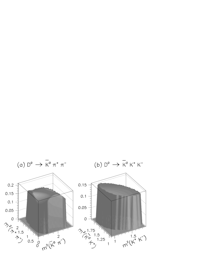
Figure 2: Efficiency on the Dalitz plot for (a) $D^{0}\rightarrow\overline{K}{}^{0}\pi^{+}\pi^{-}$ and (b) $D^{0}\rightarrow\overline{K}{}^{0}K^{+}K^{-}$.

Each Dalitz plot is divided into small cells and the efficiency distribution fit to a third-order polynomial in two dimensions. Cells with fewer than 100 generated events were ignored in the fit. The resulting $\chi^{2}$ per degree of freedom ($\chi^{2}/NDF$) is typically 1.1 using $\approx$ 500 cells. The fitted efficiencies are shown in Fig. 2. Using the weighting procedure described in the next section the weighted efficiencies values (17.94 $\pm$ 0.25)% for $\overline{K}{}^{0}\pi^{+}\pi^{-}$ and (16.56 $\pm$ 0.38)% for $\overline{K}{}^{0}K^{+}K^{-}$ are obtained. The above errors include the uncertainties on the weighting procedure.

V Branching Fractions

Since the two $K^{0}h^{+}h^{-}$ decay channels have similar topologies, the ratio of branching fractions, calculated relative to the $\overline{K}{}^{0}\pi^{+}\pi^{-}$ decay mode, is expected to have a reduced systematic uncertainty. This ratio is evaluated as

$$BR=\frac{\sum_{x,y}\frac{N_{1}(x,y)}{\epsilon_{1}(x,y)}}{\sum_{x,y}\frac{N_{0}(x,y)}{\epsilon_{0}(x,y)}},$$

where $N_{i}(x,y)$ represents the number of events measured for channel $i$, and $\epsilon_{i}(x,y)$ is the corresponding efficiency in a given Dalitz plot cell $(x,y)$ .

To obtain the yields and measure the relative branching fractions, each $\overline{K}{}^{0}h^{+}h^{-}$ mass distribution is fit assuming a double Gaussian signal and linear background where all the parameters are floated, as shown in Fig. 1(b) and Fig. 1(d). The number of signal events is calculated as the difference between the total number of events from the fit and the integrated linear background function in the same mass range. The region used is within $\pm 6\sigma$ of the $D^{0}$ mass. Selecting events within three standard deviations of the central value of the $\Delta m$ distribution, the fits give the following yields for the two channels.

$$D^{0}\rightarrow\overline{K}{}^{0}\pi^{+}\pi^{-}:\quad N=92935\pm 305$$

$$D^{0}\rightarrow\overline{K}{}^{0}K^{+}K^{-}:\quad N=13536\pm 116.$$

Systematic errors take into account effects due to the use of selection regions for the $\Delta m$ distribution, the use of particle identification, the different fitting models used to subtract the background, $K^{0}_{S}$ reconstruction, and uncertainties in the calculation of the efficiency on the Dalitz plot due to Monte Carlo statistics. The resulting systematic error is dominated by the uncertainty due to efficiency correction on the Dalitz plot.

The resulting ratio is:

$$BR=\frac{\Gamma(D^{0}\rightarrow\overline{K}{}^{0}K^{+}K^{-})}{\Gamma(D^{0}\rightarrow\overline{K}{}^{0}\pi^{+}\pi^{-})}=$$

$$(15.8\pm 0.1\;(\text{stat.})\pm 0.5\;(\text{syst.}))\times 10^{-2}$$

to be compared with the PDG value of: $(17.2\pm 1.4)\times 10^{-2}$ pdg . The best previous measurement of this branching fraction comes from the CLEO experiment (136 events for reaction (2)), which obtains the value $BR=(17.0\pm 2.2)\times 10^{-2}$ cleo2 .

The branching ratio measurements have been validated using a fully inclusive $e^{+}e^{-}\rightarrow c\bar{c}$ Monte Carlo simulation incorporating all known $D^{0}$ decay modes. The Monte Carlo events were subjected to the same reconstruction, event selection and analysis procedures as for the data. The results were found to be consistent, within statistical uncertainty, with the branching fraction values used in the Monte Carlo generation.

VI Dalitz Plot for $D^{0}\rightarrow\overline{K}{}^{0}K^{+}K^{-}$

Selecting events within $\pm 2\sigma$ of the fitted $D^{0}$ mass value, a signal fraction of 97.3% is obtained for the 12540 events selected. The Dalitz plot for these $D^{0}\rightarrow\overline{K}{}^{0}K^{+}K^{-}$ candidates is shown in Fig. 3.

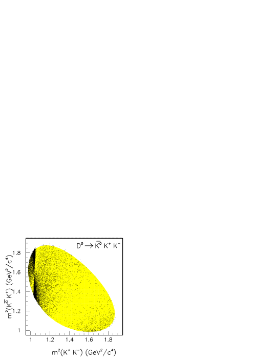
Figure 3: Dalitz plot of $D^{0}\rightarrow\overline{K}{}^{0}K^{+}K^{-}$.

In the $K^{+}K^{-}$ threshold region, a strong $\phi(1020)$ signal is observed, together with a rather broad structure. A large asymmetry with respect to the $\overline{K}{}^{0}K^{+}$ axis can also be seen in the vicinity of the $\phi(1020)$ signal, which is most probably the result of interference between $S$ and $P$-wave amplitude contributions to the $K^{+}K^{-}$ system. The $f_{0}(980)$ and $a_{0}(980)$ $S$-wave resonances are, in fact, just below the $K^{+}K^{-}$ threshold, and might be expected to contribute in the vicinity of $\phi(1020)$. An accumulation of events due to a charged $a_{0}(980)^{+}$ can be observed on the lower right edge of the Dalitz plot. This contribution, however, does not overlap with the $\phi(1020)$ region and this allows the $K^{+}K^{-}$ scalar and vector components to be separated using a partial wave analysis in the low mass $K^{+}K^{-}$ region.

VII Partial Wave Analysis

It is assumed that near threshold the production of the $K^{+}K^{-}$ system can be described in terms of the diagram shown in Fig. 4.

Figure 4: The kinematics describing the production of the $K^{+}K^{-}$ system in the threshold region.

The helicity angle, $\theta_{K}$, is then defined as the angle between the $K^{+}$ for $D^{0}$ (or $K^{-}$ for $\overline{D}{}^{0}$) in the $K^{+}K^{-}$ rest frame and the $K^{+}K^{-}$ direction in the $D^{0}$ (or $\overline{K}{}^{0}$) rest frame. The $K^{+}K^{-}$ mass distribution has been modified by weighting each $D^{0}$ candidate by the spherical harmonic $Y_{L}^{0}(\cos\theta_{K})$ (L=0-4) divided by its (Dalitz-plot-dependent) fitted efficiency. The resulting distributions $\left<Y^{0}_{L}\right>$ are shown in Fig. 5 and are proportional to the $K^{+}K^{-}$ mass-dependent harmonic moments. It is found that all the $\left<Y^{0}_{L}\right>$ moments are small or consistent with zero, except for $\left<Y^{0}_{0}\right>$, $\left<Y^{0}_{1}\right>$ and $\left<Y^{0}_{2}\right>$.

Figure 5: The unnormalized spherical harmonic moments $\left<Y^{0}_{L}\right>$ as functions of $K^{+}K^{-}$ invariant mass. The histograms represent the result of the full Dalitz plot analysis.

In order to interpret these distributions a simple partial wave analysis has been performed, involving only $S$- and $P$-wave amplitudes. This results in the following set of equations chung :

$$\sqrt{4\pi}\left<Y^{0}_{0}\right>=S^{2}+P^{2}$$

$$\sqrt{4\pi}\left<Y^{0}_{1}\right>=2\mid S\mid\mid P\mid\cos\phi_{SP}\qquad(3)$$

$$\sqrt{4\pi}\left<Y^{0}_{2}\right>=\frac{2}{\sqrt{5}}P^{2},$$

where $S$ and $P$ are proportional to the size of the $S$- and $P$-wave contributions and $\phi_{SP}$ is their relative phase. Under these assumptions, the $\left<Y^{0}_{2}\right>$ moment is proportional to $P^{2}$ so that it is natural that the $\phi(1020)$ appears free of background, as is observed. This distribution has been fit using the following relativistic $P$-wave Breit-Wigner.

For a resonance $r\rightarrow AB$, $BW(m)$ is written as

$$BW(m)=\frac{F_{r}}{m_{r}^{2}-m_{AB}^{2}-i\Gamma_{AB}m_{r}}\qquad(4)$$

where for a spin J=1 particle $F_{r}$ is the Blatt-Weisskopf damping factor dump

$$F_{r}=\frac{\sqrt{1+(Rq_{r})^{2}}}{\sqrt{1+(Rq_{AB})^{2}}}$$

and $R$ has been fixed to $R=1.5$ ${\rm GeV}^{-1}$. In Eq. (4):

$$\Gamma_{AB}=\Gamma_{r}(\frac{q_{AB}}{q_{r}})^{2J+1}(\frac{m_{r}}{m_{AB}})F^{2}_{r}$$

where $q_{AB}$ ($q_{r}$) is the momentum of either daughter in the $AB$ ($r$) rest frame.

The fit yields the following parameters:

$m_{\phi}$ = 1019.63 $\pm$ 0.07, $\Gamma_{\phi}$ = 4.28 $\pm$ 0.13 MeV/$c^{2}$

in agreement with PDG values (statistical errors only). The fit is shown in Fig. 6.

Figure 6: $\left<Y^{0}_{2}\right>$ spherical harmonic moment as a function of the $K^{+}K^{-}$ effective mass. The line is the result from the fit with a relativistic spin-1 Breit Wigner.

A strong $S-P$ interference is evidenced by the rapid motion of the $\left<Y^{0}_{1}\right>$ moment in Fig. 5 in the $\phi(1020)$ mass region.

The above system of equations (3) can be solved directly for $S^{2}$, $P^{2}$ and $\cos\phi_{SP}$. However, since these amplitudes are defined in a $D^{0}$ decay, it is necessary to correct for phase space. This has been achieved by using the $K^{+}K^{-}$ and $\overline{K}{}^{0}K^{+}$ mass spectra obtained from the Monte Carlo generation of $D^{0}$ decays to $\overline{K}{}^{0}K^{+}K^{-}$ according to phase space. The $D^{0}$ mass distribution has been generated in this Monte Carlo as a Gaussian having the experimental values of mass and mass resolution.

The phase space corrected spectra are shown in Fig. 7.

Figure 7: Results from the $K^{+}K^{-}$ Partial Wave Analysis corrected for phase space. (a) $P$-wave strength, (b) $S$-wave strength. (c) $m(\overline{K}{}^{0}K^{+})$ distribution, (d) $\cos\phi_{SP}$ in the $\phi(1020)$ region. (e) $\phi_{SP}$ in the threshold region after having subtracted the fitted $\phi(1020)$ phase motion shown in (d). The lines correspond to the fit described in the text.

The distributions have been fitted using the following model:

• The P-wave is entirely due to the $\phi(1020)$ meson (Fig. 7(a)).

• The scalar contribution in the $K^{+}K^{-}$ mass projection is entirely due to the $a_{0}(980)^{0}$ (Fig. 7(b)).

• The $\overline{K}{}^{0}K^{+}$ mass distribution is entirely due to $a_{0}(980)^{+}$ (Fig. 7(c)).

• The angle $\phi_{SP}$ (Fig. 7(d)) is obtained fitting the S, P waves and $\cos\phi_{SP}$ with $c_{a_{0}}BW_{a_{0}}+c_{\phi}BW_{\phi}e^{i\alpha}$. Here $BW_{a_{0}}$ and $BW_{\phi}$ are the Breit-Wigner describing the $a_{0}(980)$ and $\phi(1020)$ resonances.

The $a_{0}(980)$ scalar resonance has a mass very close to the $\bar{K}K$ threshold and decays mostly to $\eta\pi$. It has been described by a coupled channel Breit Wigner of the form:

$$BW_{ch}(a_{0})(m)=\frac{g_{\bar{K}K}}{m^{2}_{0}-m^{2}-i(\rho_{\eta\pi}g_{\eta\pi}^{2}+\rho_{\bar{K}K}g_{\bar{K}K}^{2})}\quad(5)$$

where $\rho(m)=2q/m$ while $g_{\eta\pi}$ and $g_{\bar{K}K}$ describe the $a_{0}(980)$ couplings to the $\eta\pi$ and $\bar{K}K$ systems respectively.

The best measurements of the $a_{0}(980)$ parameters come from the Crystal Barrel experiment cbar , in $\bar{p}p$ annihilations, and are the following:

$m_{0}$=999$\pm$2 MeV/$c^{2}$, $g_{\eta\pi}$=324$\pm$15 (MeV)^1/2, $\frac{g^{2}_{\eta\pi}}{g^{2}_{\bar{K}K}}$=1.03$\pm$0.14.

This corresponds to a value of $g_{\bar{K}K}=329\pm 27$ (MeV)^1/2.

Since in the current analysis only the $\bar{K}K$ projections are available, it is not possible to measure $m_{0}$ and $g_{\eta\pi}$. Therefore, these two quantities have been fixed to the Crystal Barrel measurements. The parameter $g_{\bar{K}K}$, on the other hand, has been left free in the fit. The result is (statistical error only):

$g_{\bar{K}K}$ = 464 $\pm$ 29 (MeV)${}^{1/2}.$

Figure 7(e) shows the residual $a_{0}(980)$ phase, obtained by first computing $\phi_{SP}$ in the range (0,$\pi$) and then subtracting the known phase motion due to the $\phi(1020)$ resonance. The fit gives a value of a relative phase $\alpha=2.12\pm 0.04$ and has a $\chi^{2}/NDF$=167/92. The fit is of rather poor quality, indicating an undetermined source of systematic uncertainty comparable with the statistical uncertainty. However the issue related to the determination of $g_{\bar{K}K}$ will be rediscussed in the complete Dalitz plot analysis described in section VIII.

The entire procedure has been tested with Monte Carlo simulations with different input values of the $a_{0}(980)$ parameters. The partial wave analysis performed on these simulated data yielded the input value of $g_{\bar{K}K}$, within the errors.

In this fit the possible presence of an $f_{0}(980)$ contribution has not been considered. This assumption can be tested by comparing the $K^{+}K^{-}$ and $\overline{K}{}^{0}K^{+}$ phase space corrected mass distributions. Since the $f_{0}(980)$ has isospin 0, it cannot decay to $\overline{K}{}^{0}K^{+}$. Therefore an excess in the $K^{+}K^{-}$ mass spectrum with respect to $\overline{K}{}^{0}K^{+}$ would indicate the presence of an $f_{0}(980)$ contribution.

Figure 8: Comparison between the phase-space-corrected $K^{+}K^{-}$ and $\overline{K}{}^{0}K^{+}$ normalised to the same area in the mass region between 0.992 and 1.05 GeV/$c^{2}$.

Figure 8 compares the $K^{+}K^{-}$ and $\overline{K}{}^{0}K^{+}$ mass distributions, normalised to the same area between 0.992 and 1.05 GeV/$c^{2}$ and corrected for phase space. It is possible to observe that the two distributions show a good agreement, supporting the argument that the $f_{0}(980)$ contribution is small. Notice that the enhanced $\overline{K}{}^{0}K^{+}$ signal level above 1.1 GeV/$c^{2}$ is the result of the $\phi(1020)$ reflection.

The resulting scalar components of the $K^{+}K^{-}$ and $\overline{K}{}^{0}K^{+}$ mass distributions, corrected for phase space, are tabulated as a function of mass in Table 1.

Table 1: $K^{+}K^{-}$ and $\overline{K}{}^{0}K^{+}$ scalar mass projections corrected for phase space in arbitrary units.

mass (GeV/$c^{2}$)	$K^{+}K^{-}$	$\overline{K}{}^{0}K^{+}$
0.988	644 $\pm$ 105
0.992	474 $\pm$ 52	575 $\pm$ 154
0.996	417 $\pm$ 37	484 $\pm$ 82
1.000	392 $\pm$ 37	414 $\pm$ 65
1.004	304 $\pm$ 35	282 $\pm$ 48
1.008	299 $\pm$ 33	331 $\pm$ 49
1.012	259 $\pm$ 39	213 $\pm$ 38
1.016	240 $\pm$ 62	235 $\pm$ 38
1.020	178 $\pm$ 84	189 $\pm$ 33
1.024	210 $\pm$ 45	153 $\pm$ 28
1.028	178 $\pm$ 30	197 $\pm$ 32
1.032	157 $\pm$ 23	129 $\pm$ 25
1.036	164 $\pm$ 19	140 $\pm$ 25
1.040	147 $\pm$ 20	102 $\pm$ 21
1.044	135 $\pm$ 17	117 $\pm$ 22
1.048	139 $\pm$ 15	132 $\pm$ 23
1.052	126 $\pm$ 13	114 $\pm$ 22
1.056	101 $\pm$ 14	119 $\pm$ 22
1.060	101 $\pm$ 12	108 $\pm$ 20
1.064	104 $\pm$ 11	72 $\pm$ 17
1.068	120 $\pm$ 12	63 $\pm$ 15

Figure 9: Dalitz plot projections for $D^{0}\rightarrow\overline{K}{}^{0}K^{+}K^{-}$. The data are represented with error bars; the histogram is the projection of the fit described in the text.

VIII Dalitz Plot Analysis of $D^{0}\rightarrow\overline{K}{}^{0}K^{+}K^{-}$.

An unbinned maximum likelihood fit has been performed for the decay $D^{0}\rightarrow\overline{K}{}^{0}K^{+}K^{-}$ in order to use the distribution of events in the Dalitz plot to determine the relative amplitudes and phases of intermediate resonant and non-resonant states.

The likelihood function has been written in the following way:

$$L=\beta\cdot G(m)\epsilon(m_{x}^{2},m_{y}^{2})\frac{\sum_{i,j}c_{i}c_{j}^{*}A_{i}A_{j}^{*}}{\int{\sum_{i,j}c_{i}c_{j}^{*}A_{i}A_{j}^{*}\epsilon(m_{x}^{2},m_{y}^{2})}dm_{x}^{2}dm_{y}^{2}}$$

$$+(1-\beta)\qquad(6)$$

In this expression, $\beta$ represents the fraction of signal obtained from the fit to the mass spectrum and $\epsilon(m_{x}^{2},m_{y}^{2})$ is the fitted efficiency on the Dalitz plot. The Gaussian function $G(m)$ describes the $D^{0}$ line shape normalised within the $\pm 2\sigma$ cutoff used to perform the Dalitz plot analysis. It is assumed that the background events, described by the second term in Eq. (6), uniformly populate the Dalitz plot. This assumption has been verified by examining events in the $D^{0}$ side bands. The output from the fit is the set of complex coefficients $c_{i}$.

In Eq. (6), the integrals have been computed using Monte Carlo events while taking into account the efficiency on the Dalitz plot. The branching fraction for the resonant or non-resonant contribution $i$ is defined by the following expression:

$$f_{i}=\frac{|c_{i}|^{2}\int|A_{i}|^{2}dm_{x}^{2}dm_{y}^{2}}{\sum_{j,k}c_{j}c_{k}^{*}\int A_{j}A_{k}^{*}dm_{x}^{2}dm_{y}^{2}}.$$

The fractions $f_{i}$ do not necessarily add up to 1 because of interference effects among the amplitudes. The errors on the fractions have been evaluated by propagating the full covariance matrix obtained from the fit.

The phase of each amplitude is measured with respect to $\overline{K}{}^{0}a_{0}(980)^{0}$ which gives the largest contribution. The amplitudes $A_{i}$ are represented by the product of complex Breit-Wigner $BW(m)$ (Eq. (4)) and angular terms $T(\mathchar 28938\relax)$ cleo :

$$A=BW(m)\times T(\mathchar 28938\relax).$$

The $f_{0}(980)$ resonance has been described using a coupled channel Breit-Wigner function with parameters taken from the WA76 wa76 , E791 e791 , and BES bes . The $a_{0}(980)$ has been parametrized using the results from the partial wave analysis discussed above.

The parameters of the $\phi(1020)$ meson have been fixed to the values obtained from the fit to the $\left<Y^{0}_{2}\right>$ moment described earlier. The non-resonant contribution (NR) is represented by a constant term with a free phase.

Systematic errors on the fitted fractions have been evaluated by making different assumptions in the fits. For example, in one test, the efficiency on the Dalitz plot has been set to a constant value. In other tests the resonance parameters of $f_{0}(980)$, $a_{0}(980)$ and $f_{0}(1400)$ have been fixed to values obtained from a variety of experiments.

The doubly-Cabibbo-suppressed contribution (DCS) $K^{+}a_{0}(980)^{-}$, whose presence should appear like an $a_{0}(980)^{-}$ in the wrong sign combination $\overline{K}{}^{0}K^{-}$, has been also included in the fit.

IX Results from the Dalitz plot analysis.

The $D^{0}\rightarrow\overline{K}{}^{0}K^{+}K^{-}$ Dalitz plot projections together with the fit results are shown in Fig. 9.

Figure 7 shows the fit projections onto the $\left<Y^{0}_{L}\right>$ moments. The fit produces a reasonable representation of the data for all of the projections. The $\chi^{2}$ computed on the Dalitz plot gives a value of $\chi^{2}/NDF$=983/774. The sum of the fractions is $130.7\pm 2.2\pm 8.4$%. The regions of higher $\chi^{2}$ are distributed rather uniformly on the Dalitz plot. Attempts to improve the fit quality by including other contributions did not give better results. One particular problem found in these fits is that including too many scalar amplitudes caused the fit to diverge, producing a sum of fractions well above 200% along with small improvements of the fit quality.

The final fit results showing fractions, amplitudes and phases are summarised in Table 2. For $\overline{K}{}^{0}f_{0}(980)$ and $K^{+}a_{0}(980)^{-}$ (DCS), being consistent with zero, only the fractions have been tabulated.

Table 2: Results from the Dalitz plot analysis of $D^{0}\rightarrow\overline{K}{}^{0}K^{+}K^{-}$. The fits have been performed using the value of $g_{\bar{K}K}=464$ (MeV)^1/2 resulting from the partial wave analysis.

Final state	Amplitude	Phase (radians)	Fraction (%)
$\overline{K}{}^{0}a_{0}(980)^{0}$	1.	0.	66.4 $\pm$ 1.6 $\pm$ 7.0
$\overline{K}{}^{0}\phi(1020)$	0.437 $\pm$ 0.006 $\pm$ 0.060	1.91 $\pm$ 0.02 $\pm$ 0.10	45.9 $\pm$ 0.7 $\pm$ 0.7
$K^{-}a_{0}(980)^{+}$	0.460 $\pm$ 0.017 $\pm$ 0.056	3.59 $\pm$ 0.05 $\pm$ 0.20	13.4 $\pm$ 1.1 $\pm$ 3.7
$\overline{K}{}^{0}f_{0}(1400)$	0.435 $\pm$ 0.033 $\pm$ 0.162	-2.63 $\pm$ 0.10 $\pm$ 0 .71	3.8 $\pm$ 0.7 $\pm$ 2.3
$\overline{K}{}^{0}f_{0}(980)$			0.4 $\pm$ 0.2 $\pm$ 0.8
$K^{+}a_{0}(980)^{-}$			0.8 $\pm$ 0.3 $\pm$ 0.8
Sum			130.7 $\pm$ 2.2 $\pm$ 8.4

The results from the Dalitz plot analysis can be summarised as follows:

• The decay is dominated by $D^{0}\rightarrow\overline{K}{}^{0}a_{0}(980)^{0}$, $D^{0}\rightarrow\overline{K}{}^{0}\phi(1020)$ and $D^{0}\rightarrow K^{-}a_{0}(980)^{+}$.

• The $f_{0}(980)$ contribution is consistent with zero, even after assuming various $f_{0}(980)$ lineshape parameters wa76  e791  bes .

• The DCS contribution is consistent with zero, regardless of the $a_{0}(980)$ parametrisation.

• The remaining contribution is not consistent with being uniform, but can be described by the tail of a broad resonance, for example the $f_{0}(1400)$ which peaks well outside the phase space. It is not possible to derive its parameters from our data, but several parametrizations have been tried, in particular those from $J/\psi$ decays bes and from $D^{+}_{s}\rightarrow\pi^{+}\pi^{+}\pi^{-}$ e791 getting in all cases improved fits.

• In one of the fits the $f_{0}(1400)$ contribution has been replaced by a non-resonant contribution, obtaining a fraction of $2.5\pm 0.5$%. However the likelihood value for this fit was worse $\Delta(2\log L)=56$.

For the $\overline{K}{}^{0}f_{0}(980)$ and DCS contributions upper limits have been computed. Combining statistical and systematic errors in quadrature, the following 95 % c.l. upper limits on the fractions have been obtained:

$$BF(D^{0}\rightarrow\overline{K}{}^{0}f_{0}(980)(\rightarrow K^{+}K^{-}))<2.1\%$$

$$BF(D^{0}\rightarrow K^{+}a_{0}(980)^{-}(\rightarrow\overline{K}{}^{0}K^{-}))(DCS)<2.5\%.$$

A test has been performed by leaving $g_{\bar{K}K}$ as a free parameter in the Dalitz plot analysis. In this test the other parameters describing the $a_{0}(980)$ ($m_{0}$ and $g_{\eta\pi}$) have been allowed to vary within their measurement errors from the Crystal Barrel experiment. The resulting central value of $g_{\bar{K}K}$ is 473 (MeV)^1/2 with a maximum deviation of 39 (MeV)^1/2, in good agreement with the value obtained using the partial wave analysis. The difference between the values, added in quadrature with the above maximum deviation, has been taken as an estimate of the systematic error:

$$g_{\bar{K}K}=473\pm 29\;(\text{stat.})\pm 40\;(\text{syst.})({\rm MeV})^{1/2}.$$

This value differs significantly from the Crystal Barrel measurement. An improvement of this measurement can be foreseen by adding data from the $a_{0}(980)\rightarrow\eta\pi$ decay mode such as $D^{0}\rightarrow K^{0}_{s}\eta\pi^{0}$. This $D^{0}$ decay mode has been studied by the CLEO cleo1 experiment (with rather limited statistics) finding a $D^{0}\rightarrow\overline{K}{}^{0}a_{0}(980)^{0}$ dominant contribution.

A large uncertainty is included in the upper limit on the presence of $f_{0}(980)$ in this $D^{0}$ decay mode due to the poor knowledge of the $f_{0}(980)$ parameters. A small signal of $f_{0}(980)$ is indeed present (in this case as a shoulder) in the $D^{0}\rightarrow\overline{K}{}^{0}\pi^{+}\pi^{-}$ as shown in Fig. 10.

Figure 10: $\pi^{+}\pi^{-}$ effective mass from $D^{0}\rightarrow\overline{K}{}^{0}\pi^{+}\pi^{-}$. The arrow indicates the position of the $f_{0}(980)$.

Dalitz plot analyses of this $D^{0}$ decay channel have been performed by BABAR gamma1 and Belle gamma2 finding ($\approx$ 5.5%) as decay fraction for $D^{0}\rightarrow\overline{K}{}^{0}f_{0}(980)$. However, a reliable estimate of the expected contribution of the $f_{0}(980)$ in $D^{0}\rightarrow\overline{K}{}^{0}K^{+}K^{-}$ decay is not possible until more accurate measurements of the $f_{0}(980)$ parameters and couplings become available. This can be performed, for example, by using high statistics samples of $D^{+}_{s}\rightarrow\bar{K}K\pi^{+}$ and $D^{+}_{s}\rightarrow\pi^{+}\pi^{+}\pi^{-}$ decays.

Table 3: Results from the Dalitz plot Analysis of $D^{0}\rightarrow\overline{K}{}^{0}K^{+}K^{-}$ separated for $D^{0}$ and $\overline{D}{}^{0}$.

Decay mode	fraction (%)	amplitude	phase (radians)	$\chi^{2}/NDF$
$D^{0}\rightarrow\overline{K}{}^{0}a_{0}(980)^{0}$	66.5 $\pm$ 2.0	1.	0.	671/649
$\overline{D}{}^{0}\rightarrow K^{0}a_{0}(980)^{0}$	66.3 $\pm$ 2.0	1.	0.	643/646
$D^{0}\rightarrow\overline{K}{}^{0}\phi(1020)$	46.3 $\pm$ 0.8	0.438 $\pm$ 0.009	1.93 $\pm$ 0.03
$\overline{D}{}^{0}\rightarrow K^{0}\phi(1020)$	45.6 $\pm$ 0.8	0.435 $\pm$ 0.009	1.88 $\pm$ 0.03
$D^{0}\rightarrow K^{-}a_{0}(980)^{+}$	13.2 $\pm$ 1.3	0.456 $\pm$ 0.025	3.58 $\pm$ 0.07
$\overline{D}{}^{0}\rightarrow K^{+}a_{0}(980)^{-}$	13.6 $\pm$ 1.3	0.463 $\pm$ 0.025	3.59 $\pm$ 0.07
$D^{0}\rightarrow\overline{K}{}^{0}f_{0}(1400)$	4.1 $\pm$ 0.9	0.451 $\pm$ 0.047	-2.58 $\pm$ 0.13
$\overline{D}{}^{0}\rightarrow K^{0}f_{0}(1400)$	3.6 $\pm$ 0.9	0.421 $\pm$ 0.038	-2.68 $\pm$ 0.14

X Search for CP asymmetries on the Dalitz plot.

A search for CP asymmetries on the Dalitz plot has been performed. Table 3 shows the results from the Dalitz plot analysis performed separately for $D^{0}$ and $\overline{D}{}^{0}$. Notice that in these two fits good values of $\chi^{2}/NDF$ have been obtained.

We do not observe any statistically significant asymmetries in fractions, amplitudes, or phases between $D^{0}$ and $\overline{D}{}^{0}$.

XI Summary

A Dalitz plot analysis of the $D^{0}$ hadronic decay $D^{0}\rightarrow\overline{K}{}^{0}K^{+}K^{-}$ has been performed. The following ratio of branching fractions has been obtained:

$$BR=\frac{\Gamma(D^{0}\rightarrow\overline{K}{}^{0}K^{+}K^{-})}{\Gamma(D^{0}\rightarrow\overline{K}{}^{0}\pi^{+}\pi^{-})}=$$

$$(15.8\pm 0.1\;(\text{stat.})\pm 0.5\;(\text{syst.}))\times 10^{-2}.$$

The Dalitz plot analysis indicates that the channel is dominated by $D^{0}\rightarrow\overline{K}{}^{0}a_{0}(980)^{0}$, $D^{0}\rightarrow\overline{K}{}^{0}\phi(1020)$ and $D^{0}\rightarrow K^{-}a_{0}(980)^{+}$. The $a_{0}(980)\rightarrow\bar{K}K$ lineshape has been extracted with little background.

The Dalitz plot analysis of $D^{0}$ and $\overline{D}{}^{0}$ do not show any statistically significant asymmetries in fractions, amplitudes, or phases.

XII Acknowledgments

We are grateful for the extraordinary contributions of our PEP-II colleagues in achieving the excellent luminosity and machine conditions that have made this work possible. The success of this project also relies critically on the expertise and dedication of the computing organizations that support BABAR. The collaborating institutions wish to thank SLAC for its support and the kind hospitality extended to them. This work is supported by the US Department of Energy and National Science Foundation, the Natural Sciences and Engineering Research Council (Canada), Institute of High Energy Physics (China), the Commissariat à l’Energie Atomique and Institut National de Physique Nucléaire et de Physique des Particules (France), the Bundesministerium für Bildung und Forschung and Deutsche Forschungsgemeinschaft (Germany), the Istituto Nazionale di Fisica Nucleare (Italy), the Foundation for Fundamental Research on Matter (The Netherlands), the Research Council of Norway, the Ministry of Science and Technology of the Russian Federation, and the Particle Physics and Astronomy Research Council (United Kingdom). Individuals have received support from CONACyT (Mexico), the A. P. Sloan Foundation, the Research Corporation, and the Alexander von Humboldt Foundation.

References

(1)
M. Bauer et al., Z. Phys. C34, 103 (1987).
(2)
E.M. Aitala et al. , Phys. Rev. Lett. 89, 121201 (2002).
E.M. Aitala et. al , Phys. Rev. Lett. 86, 770 (2001).
(3)
See for example F. E. Close and N. A. Tornqvist, J. Phys. G28, R249 (2002).
(4)
B. Aubert et al.,
Nucl. Instrum. Methods A479, 1 (2002).
(5)
GEANT, CERN Program Library, Long Writeup W5013 (1994).
(6)
S. Eidelman et al., Phys. Lett. B592, 1 (2004)
(7)
R. Ammar et al., Phys. Rev. D44, 3383 (1991).
(8)
S.U. Chung, Phys. Rev. D56, 7299 (1997).
(9)
J.M. Blatt and W.F. Weisskopf, Theoretical Nuclear Physics, John Wiley
& Sons,
New York, 1952.
(10)
A. Abele et al., Phys. Rev. D57, 3860 (1998).
(11)
S. Kopp et al., Phys. Rev. D63, 092001 (2001).
(12)
T.A. Armstrong et al., Z. Phys. C51, 351 (1991).
(13)
M. Ablikim et al.,
Phys. Lett. B607, 243 (2005).
(14)
P. Rubin et al., Phys. Rev. Lett. 93, 111801 (2004).