Amplitude Analysis of the Decay $B^{\pm}\rightarrow\mbox{$\pi^{\pm}\pi^{\pm}\pi^{\mp}$}$

Abstract

We present a Dalitz-plot analysis of charmless $B^{\pm}$ decays to the final state $\pi^{\pm}\pi^{\pm}\pi^{\mp}$ using 210 $\mbox{\,fb}^{-1}$ of data recorded by the BABAR experiment at $\sqrt{s}=10.58~{}\mathrm{\,Ge\kern-1.00006ptV}$. We measure the branching fractions ${\cal{B}}(\mbox{$B^{\pm}\rightarrow\mbox{$\pi^{\pm}\pi^{\pm}\pi^{\mp}$}$})=(16.2\pm 1.2\pm 0.9)\times 10^{-6}$ and ${\cal{B}}(B^{\pm}\rightarrow\mbox{$\mbox{$\rho^{0}$}(770)$}\pi^{\pm})=(8.8\pm 1.0\pm 0.6^{+0.1}_{-0.7})\times 10^{-6}$. Measurements of branching fractions for the quasi-two-body decays $B^{\pm}\rightarrow\mbox{$\mbox{$\rho^{0}$}(1450)$}\pi^{\pm}$, $B^{\pm}\rightarrow\mbox{$f_{0}(980)$}\pi^{\pm}$ and $B^{\pm}\rightarrow\mbox{$f_{2}(1270)$}\pi^{\pm}$ are also presented. We observe no charge asymmetries for the above modes, and there is no evidence for the decays $B^{\pm}\rightarrow\chi_{c0}\pi^{\pm}$, $B^{\pm}\rightarrow\mbox{$f_{0}(1370)$}\pi^{\pm}$ and $B^{\pm}\rightarrow\sigma\pi^{\pm}$.

I Introduction

The decay of $B$ mesons to a three-body charmless final state offers the possibility of investigating the properties of the weak interaction and provides information on the complex quark couplings described in the Cabibbo-Kobayashi-Maskawa (CKM) matrix elements CKM:1973 , as well as on models of hadronic decays. Measurements of direct $C\!P$-violating asymmetries and constraints on the magnitudes and the phases of the CKM matrix elements can be obtained from individual decay channels in $B^{\pm}\rightarrow\mbox{$\pi^{\pm}\pi^{\pm}\pi^{\mp}$}$ Gronau:1995 ; Blanco:1998 ; Blanco:2001 ; SnyderQuin:1993 , which are dominated by decays through intermediate resonances. For example, the CKM angle $\gamma$ can be extracted from the interference between the decay $B^{\pm}\rightarrow\chi_{c0}\pi^{\pm}$, which has no $C\!P$-violating phase, and other modes such as $\mbox{$\mbox{$\rho^{0}$}(770)$}\pi^{\pm}$ or $\mbox{$f_{0}(980)$}\pi^{\pm}$. Studies of these decays can also help to clarify the nature of the resonances involved, not all of which are well understood. Of particular interest is whether the $\sigma$ resonance, which has been observed in other experiments Alde ; E791 ; BESsigma , is also present in $B^{\pm}\rightarrow\mbox{$\pi^{\pm}\pi^{\pm}\pi^{\mp}$}$ decays. An analysis of the full three-body kinematic space is necessary to model the interference and extract branching fractions.

Observations of $B$-meson decays to the $\pi^{\pm}\pi^{\pm}\pi^{\mp}$ three-body final states have already been reported by the Belle and BABAR collaborations using a method that treats each intermediate decay incoherently Belle ; Babar1 . These studies have only observed $B^{\pm}\rightarrow\mbox{$\mbox{$\rho^{0}$}(770)$}\pi^{\pm}$, in which other possible resonance contributions are treated as background. The first measurement of the total branching fraction for $B^{\pm}\rightarrow\mbox{$\pi^{\pm}\pi^{\pm}\pi^{\mp}$}$ was found to be $(11\pm 4)\times 10^{-6}$ Babar2 . Here, we present results from a full amplitude analysis for $B^{\pm}\rightarrow\mbox{$\pi^{\pm}\pi^{\pm}\pi^{\mp}$}$ decay modes based on a 210.3 $\mbox{\,fb}^{-1}$ data sample containing 231.6 $\pm$ 2.6 million $B\kern 1.79993pt\overline{\kern-1.79993ptB}{}$ pairs collected with the BABAR detector babardet at the SLAC PEP-II asymmetric-energy $e^{+}e^{-}$ storage ring pep operating at the $\mathchar 28935\relax(4S)$ resonance at a center-of-mass energy of $\sqrt{s}=10.58$ $\mathrm{\,Ge\kern-1.00006ptV}$. An additional integrated luminosity of 21.6 $\mbox{\,fb}^{-1}$ was recorded $40$ $\mathrm{\,Me\kern-1.00006ptV}$ below this energy and is used to study backgrounds. The charm decay $B^{+}\rightarrow\mbox{$\kern 1.99997pt\overline{\kern-1.99997ptD}{}^{0}\pi^{+}$}$, $\kern 1.99997pt\overline{\kern-1.99997ptD}{}^{0}\rightarrow K^{+}\pi^{-}$ chargeConjugate is used as a calibration channel as it presents a relatively high branching fraction.

II The BABAR Detector

Details of the BABAR detector are described elsewhere babardet . Charged particles are measured with the combination of a silicon vertex tracker (SVT), which consists of five layers of double-sided detectors, and a 40-layer central drift chamber (DCH) in a 1.5-T solenoidal magnetic field. This provides a transverse momentum resolution for the combined tracking system of $\sigma_{p_{T}}/p_{T}=0.0013p_{T}\oplus 0.0045$, where the sum is in quadrature and $p_{T}$ is measured in ${\mathrm{\,Ge\kern-1.00006ptV\!/}c}$.

Charged-particle identification is accomplished by combining information on the specific ionization $(dE/dx)$ in the two tracking devices and the angle of emission of Cherenkov radiation in an internally reflecting ring-imaging Cherenkov detector (DIRC) covering the central region. The $dE/dx$ resolution from the drift chamber is typically about $7.5\,\%$ for pions. The Cherenkov angle resolution of the DIRC is measured to be 2.4 mrad, for the quartz refractive index of 1.473, which provides better than 3 $\sigma$ separation between charged kaons and pions over the full kinematic range of this analysis. The DIRC is surrounded by an electromagnetic calorimeter (EMC), comprising 6580 CsI(Tl) crystals, which is used to measure the energies and angular positions of photons and electrons. The EMC is used to veto electrons in this analysis.

III Event Selection and Reconstruction

Hadronic events are selected based on track multiplicity and event topology. Backgrounds from non-hadronic events are reduced by requiring the ratio of Fox-Wolfram moments $H_{2}/H_{0}$ FoxWolfram to be less than 0.98. $B$-meson candidates are reconstructed from events that have four or more charged tracks. Each track is required to be well measured and originate from the beam spot. They must have at least 12 hits in the DCH, a minimum transverse momentum of 100 ${\mathrm{\,Me\kern-1.00006ptV\!/}c}$, and a distance of closest approach to the beam spot of less than 1.5${\rm\,cm}$ in the transverse plane and less than 10${\rm\,cm}$ along the beam axis. Charged tracks identified as electrons are rejected. The $B$-meson candidates are formed from three-charged-track combinations and particle identification criteria are applied. The efficiency of selecting pions is approximately 95 %, while the probability of misidentifying kaons as pions is 15 %. The $B$-meson candidates’ energies and momenta are required to satisfy the kinematic constraints detailed in Section V.

IV Background Suppression

Backgrounds from $e^{+}e^{-}\rightarrow q\overline{q}$ are high and are suppressed by imposing requirements on event-shape variables calculated in the ${\mathchar 28935\relax\rm(4S)}$ rest frame. The first discriminating variable is $\cos{\theta_{T}}$, the cosine of the angle between the thrust axis of the selected $B$ candidate and the thrust axis of the rest of the event (all remaining charged and neutral candidates). The distribution of $\left|\cos{\theta_{T}}\right|$ is strongly peaked towards unity for $q\overline{q}$ background whereas the distribution is uniform for signal events. We require $\left|\cos{\theta_{T}}\right|$ $<0.65$. Additionally, we make requirements on a Fisher discriminant $\cal{F}$ fisher formed using a linear combination of five variables. The first two variables are the momentum-weighted Legendre polynomial moments $L_{0}=\sum_{i}p^{*}_{i}$ and $L_{2}=\sum_{i}p^{*}_{i}\times|\cos(\theta^{*}_{i})|^{2}$, where $p^{*}_{i}$ is the momentum of particle $i$ (not from the $B$ candidate) and $\theta^{*}_{i}$ is the angle between its momentum and the thrust axis of the selected $B$ candidate in the center-of-mass (CM) frame. We also use the absolute cosine of the angle between the direction of the $B$ and the collision ($z$) axis in the CM frame, as well as the magnitude of the cosine of the angle between the $B$ thrust axis and the $z$ axis in the CM frame. The last variable is the flavor of the recoiling $B$  as reported by a multivariate tagging algorithm tagging . The selection requirements placed on $\left|\cos{\theta_{T}}\right|$ and ${\cal{F}}$ are optimized using Monte Carlo simulated data and have a combined signal efficiency of 37 % while rejecting over 98 % of $q\overline{q}$  background.

Other backgrounds arise from $B\kern 1.79993pt\overline{\kern-1.79993ptB}{}$ events. The main background for our charmless signal events is from charm decays, such as three- and four-body $B$ decays involving an intermediate $D$ meson, and the charmonium decays ${J\mskip-3.0mu/\mskip-2.0mu\psi\mskip 2.0mu}\rightarrow\ell^{+}\ell^{-}$ and $\psi{(2S)}\rightarrow\ell^{+}\ell^{-}$. We remove $B$ candidates when the invariant mass of the combination of any two of its daughters tracks (of opposite charge) is within the ranges $3.05<m_{\pi^{+}\pi^{-}}<3.22{\mathrm{\,Ge\kern-1.00006ptV\!/}c^{2}}$, $3.68<m_{\pi^{+}\pi^{-}}<3.87{\mathrm{\,Ge\kern-1.00006ptV\!/}c^{2}}$ and $1.70<m_{\pi^{+}\pi^{-}}<1.93{\mathrm{\,Ge\kern-1.00006ptV\!/}c^{2}}$, which reject the decays ${J\mskip-3.0mu/\mskip-2.0mu\psi\mskip 2.0mu}\rightarrow\ell^{+}\ell^{-}$, $\psi{(2S)}\rightarrow\ell^{+}\ell^{-}$  and $\kern 1.99997pt\overline{\kern-1.99997ptD}{}^{0}\rightarrow K^{+}\pi^{-}$ (or $\pi^{+}\pi^{-}$), respectively. These ranges are asymmetric about the nominal masses pdg2004 in order to remove decays in which a lepton ($\ell$) or kaon has been misidentified as a pion.

We study the remaining backgrounds from charmless $B$ decays and from charm decays that escape the vetoes using a large sample of Monte Carlo (MC) simulated $B\kern 1.79993pt\overline{\kern-1.79993ptB}{}$ decays equivalent to approximately five times the integrated luminosity for the data. Any events that pass the selection criteria are further studied using exclusive MC samples to estimate reconstruction efficiency and yields. We find that the only significant background arises from $B^{\pm}\rightarrow\mbox{$K^{\pm}\pi^{\mp}\pi^{\pm}$}$ decays, in which the kaon has been misidentified as a pion.

We also consider the decay $B^{\pm}\rightarrow K^{0}_{\scriptscriptstyle S}\pi^{\pm}$, ${K^{0}_{\scriptscriptstyle S}}\rightarrow\pi^{+}\pi^{-}$ to be a background, since the $K^{0}_{\scriptscriptstyle S}$ candidates decay weakly and do not interfere with other $\pi^{+}\pi^{-}$ resonances in $B^{\pm}\rightarrow\mbox{$\pi^{\pm}\pi^{\pm}\pi^{\mp}$}$. We suppress this background by fitting two oppositely charged pions from each $B$ candidate to a common vertex when the invariant mass of the pair is below 0.6 ${\mathrm{\,Ge\kern-1.00006ptV\!/}c^{2}}$. This vertex corresponds to the $K^{0}_{\scriptscriptstyle S}$ decay point for true ${K^{0}_{\scriptscriptstyle S}}\rightarrow\pi^{+}\pi^{-}$ candidates. We remove $B$ decays that have fitted $K^{0}_{\scriptscriptstyle S}$ candidates with masses between 476 and 519 ${\mathrm{\,Me\kern-1.00006ptV\!/}c^{2}}$ ($\sigma=3.6~{}{\mathrm{\,Me\kern-1.00006ptV\!/}c^{2}}$).

A further background in this analysis comes from signal events that have been misreconstructed by switching one or more particles from the decay of the signal $B$ meson with particles from the other $B$ meson in the event. The amount of this background is estimated from MC studies and is found to be very small; it accounts for 0.6 % of the final data sample in the signal region (defined in Section V) and is therefore neglected in this analysis.

V Final Data Selection

Two kinematic variables are used to select the final data sample. The first variable is $\mbox{$\Delta E$}=E_{B}^{*}-\sqrt{s}/2$, the difference between the CM energy of the $B$-meson candidate and $\sqrt{s}/2$, where $\sqrt{s}$ is the total CM energy. The second is the energy-substituted mass $m_{\rm ES}$ $=\sqrt{(s/2+{\bf p}_{i}\cdot{\bf p}_{B})^{2}/E_{i}^{2}-{\bf p}^{2}_{B}}$ where ${\bf p}_{B}$ is the $B$ momentum and ($E_{i}$,p_i) is the four-momentum of the initial state in the laboratory frame. For signal $B$ decays, the $\Delta E$ distribution peaks near zero with a resolution of 19 $\mathrm{\,Me\kern-1.00006ptV}$, while the $m_{\rm ES}$ distribution peaks near the $B$ mass with a resolution of 2.7 ${\mathrm{\,Me\kern-1.00006ptV\!/}c^{2}}$. The mean of the $\Delta E$ distribution is shifted by $-5$ $\mathrm{\,Me\kern-1.00006ptV}$ from zero in data as measured from the calibration channel $B^{+}\rightarrow\mbox{$\kern 1.99997pt\overline{\kern-1.99997ptD}{}^{0}\pi^{+}$}$, $\kern 1.99997pt\overline{\kern-1.99997ptD}{}^{0}\rightarrow K^{+}\pi^{-}$  assuming the kaon hypothesis for the $K^{+}$ candidate. The same shift is also observed for $B^{+}\rightarrow\mbox{$\kern 1.99997pt\overline{\kern-1.99997ptD}{}^{0}\pi^{+}$}$, $\kern 1.99997pt\overline{\kern-1.99997ptD}{}^{0}\rightarrow\pi^{+}\pi^{-}$. The typical $\Delta E$ separation between modes that differ by substituting a kaon for a pion in the final state is 45 $\mathrm{\,Me\kern-1.00006ptV}$, assuming the pion mass hypothesis. Events in the $\Delta E$ strip $-65<\mbox{$\Delta E$}<55$ $\mathrm{\,Me\kern-1.00006ptV}$ are accepted. We also require events to lie in the range $5.20<\mbox{$m_{\rm ES}$}<5.29$ ${\mathrm{\,Ge\kern-1.00006ptV\!/}c^{2}}$. This range is used for an extended maximum likelihood fit to the $m_{\rm ES}$  distribution in order to determine the fraction of signal and background events in our data sample. The region is further subdivided into two areas: we use the sideband region ($5.20<\mbox{$m_{\rm ES}$}<5.26$ ${\mathrm{\,Ge\kern-1.00006ptV\!/}c^{2}}$) to study the background Dalitz-plot distribution and the signal region ($5.271<\mbox{$m_{\rm ES}$}<5.287$ ${\mathrm{\,Ge\kern-1.00006ptV\!/}c^{2}}$) to perform the Dalitz-plot analysis. We accept one $B$-meson candidate per event in the $\Delta E$ strip. Fewer than 3 % of events have multiple candidates and in those events one candidate is randomly accepted to avoid bias.

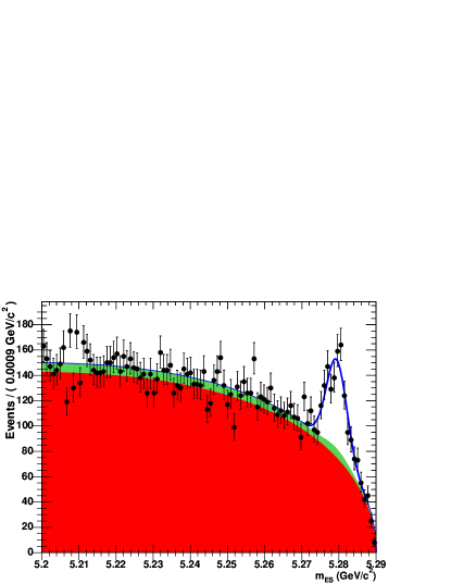
Figure 1: The $m_{\rm ES}$ distribution along the $\Delta E$ strip ($-65<\mbox{$\Delta E$}<55$ $\mathrm{\,Me\kern-1.00006ptV}$): the data are the black points with statistical error bars, the lower solid red (dark) area is the $q\overline{q}$ component, the middle solid green (light) area is the $B\kern 1.79993pt\overline{\kern-1.79993ptB}{}$ background contribution, while the upper blue line shows the total fit result.

The $m_{\rm ES}$ signal component is modeled by a Gaussian function, while the $q\overline{q}$ background is modeled using the ARGUS function argus with the endpoint fixed to the beam energy while the shape parameter is allowed to float. The $B\kern 1.79993pt\overline{\kern-1.79993ptB}{}$ background $m_{\rm ES}$ shape is modeled with an ARGUS function plus a Gaussian to account for the dominant peaking $B\kern 1.79993pt\overline{\kern-1.79993ptB}{}$ background of $86\pm 9$ $B^{\pm}\rightarrow\mbox{$K^{\pm}\pi^{\mp}\pi^{\pm}$}$ events, as well as $7\pm 1$ $B^{\pm}\rightarrow K^{0}_{\scriptscriptstyle S}\pi^{\pm}$ events that have $K^{0}_{\scriptscriptstyle S}$ candidates with invariant masses outside the 6$~{}\sigma$ range. All parameters of the $B\kern 1.79993pt\overline{\kern-1.79993ptB}{}$ component, including the amount of peaking and nonpeaking $B\kern 1.79993pt\overline{\kern-1.79993ptB}{}$ background, are obtained and fixed from the MC simulation. The fraction of $q\overline{q}$ events is allowed to float. Figure 1 shows the $m_{\rm ES}$ projection of the fit to the data for $B^{\pm}\rightarrow\mbox{$\pi^{\pm}\pi^{\pm}\pi^{\mp}$}$. The $\chi^{2}$ per degree of freedom for this projection is 93/95 and the total number of events in the signal region is 1942 (965 and 977 for the $B^{-}$ and $B^{+}$ samples, respectively). In the signal region, the fraction of $q\overline{q}$ background $f_{q\overline{q}}$ is found to be $(71.2\pm 1.8)$ %, while the fraction of $B\kern 1.79993pt\overline{\kern-1.79993ptB}{}$ backgrounds $f_{B\kern 1.25995pt\overline{\kern-1.25995ptB}{}}$ is $(4.7\pm 0.5)$ %. The fraction of signal events in the signal region is then $f_{\rm{sig}}=1-f_{q\overline{q}}-f_{B\kern 1.25995pt\overline{\kern-1.25995ptB}{}}=(24.1\pm 1.8)$ %.

VI Dalitz Amplitude Analysis

The charmless $B$-meson decay to the final state $\pi^{\pm}\pi^{\pm}\pi^{\mp}$ has a number of intermediate states in the Dalitz plot Dalitz that contribute to the total rate, which can be represented in the form:

$$\frac{d\Gamma}{ds_{13}ds_{23}}=|{\cal{M}}|^{2}\propto\left|\sum_{k}c_{k}e^{i\theta_{k}}{\cal{D}}_{k}(s_{13},s_{23})\right|^{2}$$ (1)

where $s_{13}=m_{\pi^{+}\pi^{-}}^{2}$ and $s_{23}=m_{\pi^{+}\pi^{-}}^{2}$ are the invariant masses squared of the oppositely-charged pion pairs in the final state. The invariant mass of each $B$ candidate is constrained to the world-average value pdg2004 before $s_{13}$ and $s_{23}$ are calculated. The amplitude for a given decay mode $k$ is proportional to $c_{k}e^{i\theta_{k}}{\cal{D}}_{k}(s_{13},s_{23})$ with magnitude $c_{k}$ and phase $\theta_{k}$ ($-\pi\leq\theta_{k}\leq\pi$). The distributions ${\cal{D}}_{k}$ describe the dynamics of the decay and are a product of the invariant mass and angular distributions. For example, if we have a resonance formed from the first and third pion from $B^{\pm}\rightarrow\mbox{$\pi^{\pm}\pi^{\pm}\pi^{\mp}$}$, then

$${\cal{D}}_{k}(s_{13},s_{23})=R_{k}(s_{13})\times T_{k}(s_{13},s_{23}),$$ (2)

where $R_{k}(s_{13})$ is the resonance mass distribution and $T_{k}(s_{13},s_{23})$ is the angular-dependent amplitude. The ${\cal{D}}_{k}$ are normalized such that

$$\int|{\cal{D}}_{k}(s_{13},s_{23})|^{2}ds_{13}ds_{23}=1.$$ (3)

The distribution $R_{k}(s_{13})$ is taken to be a relativistic Breit–Wigner lineshape with Blatt–Weisskopf barrier factors blatt for all resonances in this analysis except for the $f_{0}(980)$, which is modeled with a Flatté lineshape flatte to account for its coupled-channel behavior because it couples also to the $K^{+}K^{-}$ channel right at threshold. The nonresonant component is assumed to be uniform in phase space. The Breit–Wigner function has the form

$$R_{k}(s_{13})=\frac{1}{m^{2}_{0}-s_{13}-im_{0}\Gamma(s_{13})},$$ (4)

where $m_{0}$ is the nominal mass of the resonance and $\Gamma(s_{13})$ is the mass-dependent width. In the general case, the latter can be modeled as

$$\Gamma(s_{13})=\Gamma_{0}\left(\frac{q}{q_{0}}\right)^{2J+1}\frac{m_{0}}{\sqrt{s_{13}}}\frac{X^{2}_{J}(q)}{X^{2}_{J}(q_{0})}.$$ (5)

The symbol $\Gamma_{0}$ denotes the nominal width of the resonance. The values of $m_{0}$ and $\Gamma_{0}$ are obtained from standard tables pdg2004 . The value $q$ is the momentum of either daughter in the rest frame of the resonance, and is given by

$$q=\sqrt{[s_{13}-(m^{2}_{1}+m^{2}_{3})][s_{13}-(m^{2}_{1}-m^{2}_{3})]/4s_{13}},$$ (6)

where $m_{1}$ and $m_{3}$ are the masses of the two daughter particles, respectively. The symbol $q_{0}$ denotes the value of $q$ when $s_{13}=m^{2}_{0}$. The Blatt–Weisskopf barrier penetration factor $X_{J}(q)$ depends on the momentum $q$ as well as on the spin of the resonance $J$ blatt :

$$X_{0}(z) = 1,$$ (7)

$$X_{1}(z) = \sqrt{1/(1+z^{2})},$$ (8)

$$X_{2}(z) = \sqrt{1/(z^{4}+3z^{2}+9)},$$ (9)

where $z=rq$ and $r$ is the radius of the barrier, which we take to be 4 GeV^-1 (equivalent to the approximate size of 0.8 fm).

In the case of the Flatté lineshape flatte , which is used to describe the dynamics of the $f_{0}(980)$ resonance, the mass-dependent width is given by the sum of the widths in the $\pi\pi$ and $KK$ systems:

$$\Gamma(s_{13})=\Gamma_{\pi}(s_{13})+\Gamma_{K}(s_{13}),$$ (10)

where

$$\Gamma_{\pi}(s_{13}) = g_{\pi}\sqrt{s_{13}-4m^{2}_{\pi}},$$

$$\Gamma_{K}(s_{13}) = g_{K}\sqrt{s_{13}-4m^{2}_{K}}$$ (11)

and $g_{\pi}$ and $g_{K}$ are effective coupling constants, squared, for $\mbox{$f_{0}(980)$}\rightarrow\pi\pi$ and $\mbox{$f_{0}(980)$}\rightarrow KK$, respectively. We use the values $g_{\pi}=0.138$ and $g_{K}=4.45g_{\pi}$ obtained by the BES collaboration BESsigma .

We use the Zemach tensor formalism Zemach for the angular distributions $T^{(J)}_{k}$ of a spin 0 particle ($B^{\pm}$) decaying into a spin $J$ resonance and a spin 0 bachelor particle ($\pi^{\pm}$). For $J=0,1,2$, we have Zemachpdg :

$$T^{(0)}_{k} = 1,$$

$$T^{(1)}_{k} = -2\vec{p}\cdot\vec{q},$$

$$T^{(2)}_{k} = \frac{4}{3}\left[3(\vec{p}\cdot\vec{q})^{2}-(|\vec{p}||\vec{q}|)^{2}\right],$$ (12)

where $\vec{p}$ is the momentum of the bachelor particle and $\vec{q}$ is the momentum of the like-sign resonance daughter, both measured in the rest frame of the resonance.

To fit the data in the signal region, we define an unbinned likelihood function for each event to have the form

$${\cal{L}}(s_{13},s_{23})=f_{\rm{sig}}$$

$$\frac{|\sum_{k=1}^{n}c_{k}e^{i\theta_{k}}{\cal{D}}_{k}(s_{13},s_{23})|^{2}\epsilon(s_{13},s_{23})}{\int~{}{|\sum_{k=1}^{n}c_{k}e^{i\theta_{k}}{\cal{D}}_{k}(s_{13},s_{23})|^{2}\epsilon(s_{13},s_{23})}~{}ds_{13}ds_{23}}$$

$$+~{}f_{q\bar{q}}~{}\frac{Q(s_{13},s_{23})}{\int~{}Q(s_{13},s_{23})~{}ds_{13}ds_{23}}$$

$$+~{}f_{B\bar{B}}~{}\frac{B(s_{13},s_{23})}{\int~{}B(s_{13},s_{23})~{}ds_{13}ds_{23}}$$ (13)

where $n$ is the total number of resonant and nonresonant components in the signal model; $\epsilon(s_{13},s_{23})$ is the signal reconstruction efficiency defined for all points in the Dalitz plot; $Q(s_{13},s_{23})$ is the distribution of $q\overline{q}$ background; $B(s_{13},s_{23})$ is the distribution of $B\kern 1.79993pt\overline{\kern-1.79993ptB}{}$ background; and $f_{\rm{sig}}$, $f_{q\overline{q}}$ and $f_{B\kern 1.25995pt\overline{\kern-1.25995ptB}{}}$ are the fractions of signal, $q\overline{q}$ and $B\kern 1.79993pt\overline{\kern-1.79993ptB}{}$ backgrounds, respectively. Since we have two identical pions in the final state, the dynamical amplitudes, signal efficiency and background distributions are symmetrized between $s_{13}$ and $s_{23}$. The fit is performed allowing the amplitude magnitudes ($c_{i}$) and the phases ($\theta_{i}$) to vary.

The first term on the right-hand-side in Eq. (VI) corresponds to the signal probability density function (PDF) multiplied by the signal fraction $f_{\rm{sig}}$. This analysis will only be sensitive to relative phases and magnitudes, since we can always apply a common magnitude scaling factor and phase transformation to all terms in the numerator and denominator of the signal PDF. Therefore, we have fixed the magnitude and phase of the most dominant component, $\mbox{$\rho^{0}$}(770)$, to be 1 and 0, respectively.

As the choice of normalization, phase convention and amplitude formalism may not always be the same for different experiments, fit fractions are also presented to allow a more meaningful comparison of results. The fit fraction for resonance $k$, $F_{k}$, is defined as the integral of a single decay amplitude squared divided by the coherent matrix element squared for the complete Dalitz plot as shown in Eq. (14).

$$F_{k}=\frac{\int|c_{k}e^{i\theta_{k}}{\cal{D}}_{k}(s_{13},s_{23})|^{2}ds_{13}ds_{23}}{\int|\sum_{j}c_{j}e^{i\theta_{j}}{\cal{D}}_{j}(s_{13},s_{23})|^{2}ds_{13}ds_{23}},$$ (14)

where the integrals are performed over the full kinematic range. Note that the sum of these fit fractions is not necessarily unity due to the potential presence of net constructive or destructive interference.

VII Dalitz Plot Backgrounds and Efficiency

The dominant source of background for this analysis comes from $q\overline{q}$ events. We use a combination of on-resonance sideband data and off-resonance data to get the background distribution for the Dalitz plot. Note that for the on-resonance sideband data, we subtract any contributions from $B\kern 1.79993pt\overline{\kern-1.79993ptB}{}$ background (from MC), since this is handled separately. Since the background peaks at the edges of the Dalitz plot, we use a coordinate transformation to a square Dalitz plot in order to improve the modeling of the background distribution. Considering the decay $B^{+}\rightarrow\pi^{+}\pi^{+}\pi^{-}$, the new coordinates are $m^{\prime}$ and $\theta^{\prime}$, which are defined as

$$m^{\prime} = \frac{1}{\pi}\cos^{-1}\left(2\frac{m_{++}-m_{++}\rm{[min]}}{m_{++}{\rm{[max]}}-m_{++}\rm{[min]}}-1\right),$$

$$\theta^{\prime} = \frac{1}{\pi}\theta_{++},$$ (15)

where $m_{++}$ is the invariant mass of the like-sign pions, $m_{++}{\rm{[max]}}=m_{B}-m_{\pi}$ and $m_{++}{\rm{[min]}}=2m_{\pi}$ are the boundaries of $m_{++}$, while $\theta_{++}$ is the helicity angle between the momentum of one of the like-sign ($\pi^{+}$) pions and the $\pi^{-}$ momentum in the $\pi^{+}\pi^{+}$ rest-frame. Note that the new variables range from 0 to 1. The Jacobian transformation $J$ between the normal Dalitz plot variables to the new coordinates is defined as

$$ds_{13}ds_{23}=|J|dm^{\prime}d\theta^{\prime}.$$ (16)

The determinant $|J|$ of the Jacobian is given by

$$|J|=4|p_{1}^{*}||p_{2}^{*}|m_{++}\frac{\partial m_{++}}{\partial m^{\prime}}\frac{\partial\cos\theta_{++}}{\partial\theta^{\prime}},$$ (17)

where $|p^{*}_{1}|$ is the momentum of one of the $\pi^{+}$ candidates and $|p^{*}_{2}|$ is the momentum of the $\pi^{-}$ track, both measured in the rest frame of the $\pi^{+}\pi^{+}$ system. The partial derivatives in Eq. (17) are given by

$$\frac{\partial m_{++}}{\partial m^{\prime}} = -\frac{\pi}{2}\sin(\pi m^{\prime})(m_{++}{\rm{[max]}}-m_{++}{\rm{[min]}}),$$

$$\frac{\partial\cos\theta_{++}}{\partial\theta^{\prime}} = -\pi\sin(\pi\theta^{\prime}).$$ (18)

We get similar expressions for $B^{-}\rightarrow\pi^{-}\pi^{-}\pi^{+}$. Figure 2 shows the $q\overline{q}$ background distribution, obtained by combining on-resonance sideband and off-resonance data. Figure 3 shows the $B\kern 1.79993pt\overline{\kern-1.79993ptB}{}$ background distributions, which originate from $B^{\pm}\rightarrow\mbox{$K^{\pm}\pi^{\mp}\pi^{\pm}$}$ and $B^{\pm}\rightarrow K^{0}_{\scriptscriptstyle S}\pi^{\pm}$ decays. Note that the peaks along the edges of the normal Dalitz plot distribution are more spread out in the square Dalitz plot format. We use the latter to represent the $q\overline{q}$  and $B\kern 1.79993pt\overline{\kern-1.79993ptB}{}$ backgrounds in the amplitude fit, applying linear interpolation between bins.

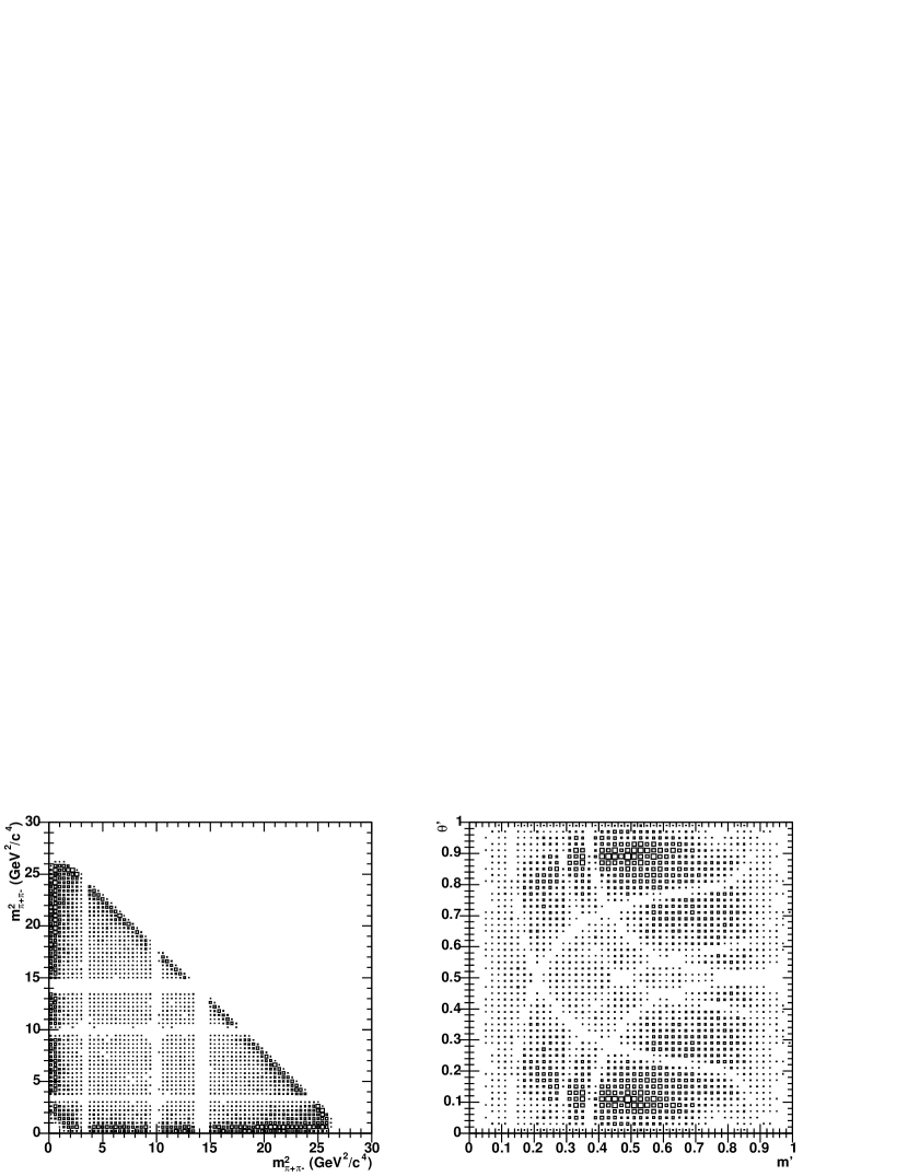
Figure 2: Dalitz plot of the $q\overline{q}$ background obtained from on-resonance sideband and off-resonance data. The left plot shows the distribution in normal Dalitz plot coordinates, while the right plot shows the equivalent distribution in the new square Dalitz plot coordinates, defined in Eq. (VII). The empty regions correspond to events removed by the charm vetoes. The area of each small square is proportional to the number of events in that bin.

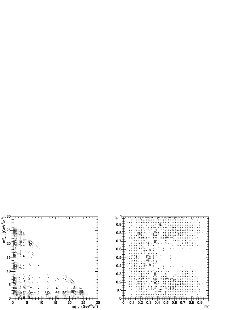
Figure 3: Dalitz plot of the $B\kern 1.79993pt\overline{\kern-1.79993ptB}{}$ background obtained from Monte Carlo simulated events. The left plot shows the distribution in normal Dalitz plot coordinates, while the right plot shows the equivalent distribution in the new square Dalitz plot coordinates, defined in Eq. (VII). The empty regions correspond to events removed by the charm vetoes. The area of each small square is proportional to the number of events in that bin.

The signal efficiency $\epsilon(s_{13},s_{23})$ used in Eq. (VI) is modeled using a two-dimensional histogram with bins of size $0.4~{}({\mathrm{\,Ge\kern-1.00006ptV\!/}c^{2}})^{2}\times 0.4~{}({\mathrm{\,Ge\kern-1.00006ptV\!/}c^{2}})^{2}$ and is obtained using 1.1 million $B^{\pm}\rightarrow\mbox{$\pi^{\pm}\pi^{\pm}\pi^{\mp}$}$ nonresonant MC events. All selection criteria are applied except for those corresponding to the invariant-mass veto regions mentioned in Sec. IV. The efficiency at a given bin is defined as the ratio of the number of events reconstructed to the number of events generated in that bin. Corrections for differences between MC and data in the particle identification and tracking efficiencies are applied. The efficiency shows little variation across the majority of the Dalitz plot, in which the average efficiency is measured to be $(13.00\pm 0.04)\,\%$, however there are decreases towards the corners where one of the particles has a low momentum. The effect of experimental resolution on the signal model is neglected since the resonances under consideration are sufficiently broad. No difference in efficiency is seen between $B^{-}$ and $B^{+}$ decays at the 2% level.

VIII Physics Results

We fit the $B^{-}$ and $B^{+}$ samples independently to extract the magnitudes and phases of the resonant and nonresonant contributions to the charmless $B^{\pm}\rightarrow\mbox{$\pi^{\pm}\pi^{\pm}\pi^{\mp}$}$ Dalitz plot, using Eq. (VI). The nominal fit model contains the resonances $\mbox{$\rho^{0}$}(770)$, $\mbox{$\rho^{0}$}(1450)$, $f_{0}(980)$, $f_{2}(1270)$ and a uniform nonresonant contribution. This is chosen using information from established resonance states pdg2004 and the $\chi^{2}$ variation observed when omitting one of the five components. The $\chi^{2}$ value is calculated using the formula

$$\chi^{2}=\sum_{i=1}^{n_{b}}\frac{[y_{i}-f(x_{i})]^{2}}{\sigma_{i}^{2}},$$ (19)

where $y_{i}$ is the number of events in bin $i$ of the invariant mass or Dalitz-plot distribution, $f(x_{i})$ is the expected number of events in that bin as predicted by the fit result and $\sigma_{i}$ is the error on $y_{i}$ ($\sqrt{y_{i}}$). The number of degrees of freedom (nDof) is calculated as $n_{b}-k-1$, where $n_{b}$ is the total number of bins used and $k$ is the number of free parameters in the fit (4 magnitudes and 4 phases). A minimum of 10 entries in each bin is required; if this requirement is not met then neighboring bins are combined. Typically, $n_{b}$ is equal to 35 and 75 for the invariant mass and Dalitz-plot distributions, respectively. Since we observe no charge asymmetry in the $q\overline{q}$ and $B\kern 1.79993pt\overline{\kern-1.79993ptB}{}$ backgrounds, we use the charge-averaged background distributions shown in Figs. 2 and 3 for the $B^{-}$ and $B^{+}$ fits. The results of the nominal fit to $B^{-}$ and $B^{+}$ on-resonance data in the signal region are shown separately in Table 1.

Table 1: Results of the nominal fits to $B^{-}\rightarrow\mbox{$\pi^{-}\pi^{-}\pi^{+}$}$ and $B^{+}\rightarrow\mbox{$\pi^{+}\pi^{+}\pi^{-}$}$ data. The first errors are statistical, while the second and third uncertainties are systematic and model-dependent, respectively, all of which are detailed in Sec. IX. All phases are in radians.

Component		$B^{-}$ Fit Result		$B^{+}$ Fit Result
$\mbox{$\rho^{0}$}(770)$ Fraction (%)		$50.6\pm 7.3\pm 2.2^{+0.4}_{-2.7}$		$57.8\pm 6.8\pm 3.5^{+1.0}_{-7.9}$
$\mbox{$\rho^{0}$}(770)$ Magnitude		1.0 (fixed)		1.0 (fixed)
$\mbox{$\rho^{0}$}(770)$ Phase		0.0 (fixed)		0.0 (fixed)
$\mbox{$\rho^{0}$}(1450)$ Fraction (%)		$6.8\pm 4.5\pm 1.8\pm 0.6$		$4.9\pm 5.5\pm 1.4^{+0.8}_{-2.3}$
$\mbox{$\rho^{0}$}(1450)$ Magnitude		$0.37\pm 0.11\pm 0.05\pm 0.02$		$0.29\pm 0.17\pm 0.06\pm 0.08$
$\mbox{$\rho^{0}$}(1450)$ Phase		$+1.99\pm 0.57\pm 0.10\pm 0.08$		$+0.31\pm 0.70\pm 0.15\pm 0.34$
$f_{0}(980)$ Fraction (%)		$3.8\pm 4.9\pm 0.9\pm 2.1$		$11.1\pm 5.1\pm 1.1^{+4.4}_{-3.4}$
$f_{0}(980)$ Magnitude		$0.27\pm 0.10\pm 0.05\pm 0.07$		$0.44\pm 0.12\pm 0.03\pm 0.08$
$f_{0}(980)$ Phase		$-1.59\pm 0.47\pm 0.08^{+0.15}_{-0.01}$		$-0.79\pm 0.62\pm 0.17^{+0.15}_{-0.02}$
$f_{2}(1270)$ Fraction (%)		$14.2\pm 4.6\pm 1.3\pm 0.5$		$14.1\pm 4.8\pm 1.4^{+0.7}_{-3.1}$
$f_{2}(1270)$ Magnitude		$0.53\pm 0.10\pm 0.02\pm 0.03$		$0.49\pm 0.11\pm 0.02\pm 0.05$
$f_{2}(1270)$ Phase		$+1.39\pm 0.41\pm 0.09\pm 0.09$		$+1.85\pm 0.47\pm 0.12^{+0.39}_{-0.07}$
Nonresonant Fraction (%)		$15.0\pm 8.6\pm 1.9^{+4.3}_{-1.3}$		$12.6\pm 7.1\pm 2.6^{+1.1}_{-4.3}$
Nonresonant Magnitude		$0.54\pm 0.13\pm 0.03\pm 0.09$		$0.47\pm 0.14\pm 0.05\pm 0.06$
Nonresonant Phase		$-0.84\pm 0.38\pm 0.06\pm 0.04$		$-2.80\pm 0.46\pm 0.07\pm 0.07$

From Eq. (14), it can be seen that the fit fraction statistical uncertainty will not only depend on the uncertainties of the magnitude and phase of the given resonance, but also on the statistical errors of all amplitudes. Therefore, we use a MC pseudo-experiment technique to obtain the statistical uncertainty on each fit fraction. Each pseudo-experiment is a sample of MC generated events that contains the correct mixture of signal and background, which are distributed across the Dalitz plot according to the PDFs defined in Eq. (VI). We fit these MC samples and plot the distributions of fit fractions $F_{k}$ obtained from a thousand such experiments. The statistical uncertainty for each $F_{k}$ is then the value of the width of the Gaussian function that is fitted to the $F_{k}$ distribution.

Figure 4 shows the mass projection plots for the nominal fits to $B^{-}$ and $B^{+}$ data, while Fig. 5 shows the background-subtracted Dalitz plot of the combined $B^{\pm}\rightarrow\mbox{$\pi^{\pm}\pi^{\pm}\pi^{\mp}$}$ data in the signal region. The $\chi^{2}$/nDof values for the opposite-sign and like-sign invariant mass projections for $B^{-}$ ($B^{+}$) are 51/34 and 27/37 (35/35 and 47/35), respectively. The $\chi^{2}$/nDof values for the two-dimensional Dalitz plots are 74/74 and 70/75 for $B^{-}$ and $B^{+}$, respectively. The four resonant contributions plus the single uniform phase-space nonresonant model are able to describe the data adequately within the statistical uncertainties.

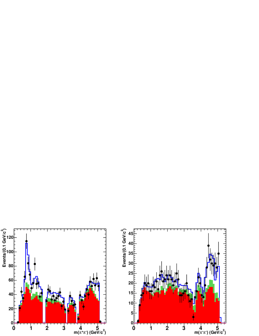
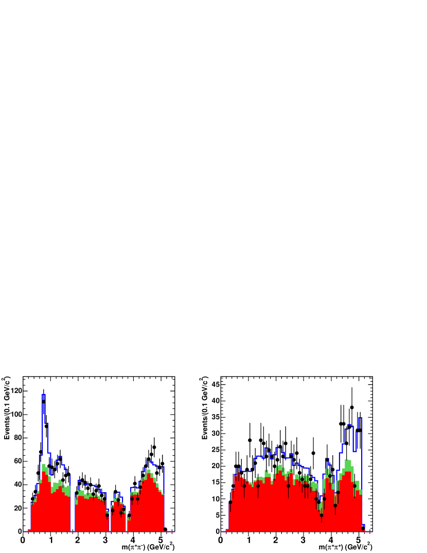
Figure 4: Projection plots of the fit results for $B^{-}\rightarrow\mbox{$\pi^{-}\pi^{-}\pi^{+}$}$ and $B^{+}\rightarrow\mbox{$\pi^{+}\pi^{+}\pi^{-}$}$ onto the mass variables $m_{\pi^{+}\pi^{-}}$ and $m_{\pi^{-}\pi^{-}}$ ($m_{\pi^{+}\pi^{+}}$). The upper (lower) plots are for the $B^{-}$ ($B^{+}$) data sample. The data are the black points with statistical error bars, the lower solid red (dark) histogram is the $q\overline{q}$ component, the middle solid green (light) histogram is the $B\kern 1.79993pt\overline{\kern-1.79993ptB}{}$ background contribution, while the upper blue histogram shows the total fit result. The large dips in the spectra correspond to the charm vetoes.

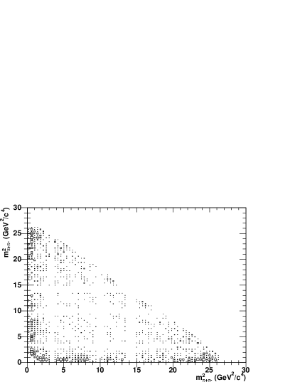
Figure 5: Background subtracted Dalitz plot of the combined $B^{\pm}\rightarrow\mbox{$\pi^{\pm}\pi^{\pm}\pi^{\mp}$}$ data sample in the signal region. The Dalitz plot is symmetrized about the $y=x$ axis. The empty regions correspond to events removed by the charm vetoes.

For a given resonance, the comparison of the fit fraction, not the magnitude, to its uncertainty gives a measure of how significant its contribution is to the Dalitz plot. Note that the fit fraction uncertainties shown in Table 1 are larger than the uncertainties of the magnitudes. This is due to the dependence of the former on all of the other amplitudes, via the denominator in Eq. (14). It can be clearly seen that the dominant contribution to the charmless $B^{\pm}\rightarrow\mbox{$\pi^{\pm}\pi^{\pm}\pi^{\mp}$}$ Dalitz plot is from the $\mbox{$\rho^{0}$}(770)$ resonance. Approximately 10 % of the $\mbox{$\rho^{0}$}(770)$ fit fraction lies in the tail of the mass distribution, defined as the region outside $m_{0}\pm 3\Gamma_{0}$. In addition, the fraction of $\mbox{$\rho^{0}$}(770)$ within one width of the $f_{2}(1270)$ resonance line-shape is approximately 13 %, which is equivalent to half of the $f_{2}(1270)$ fit fraction. Further fits are performed to the data by removing one two-body component at a time from the nominal model. Removing the $\mbox{$\rho^{0}$}(770)$, $f_{2}(1270)$ or nonresonant components give significantly poorer fit results. Omitting the $\mbox{$\rho^{0}$}(1450)$ or $f_{0}(980)$ components, which are present at the $1.5~{}\sigma$ level, gives a small change in the goodness-of-fit $\chi^{2}$ (Eq. (19)).

We have also tested the introduction of the $\chi_{c0}$ and $f_{0}(1370)$ resonances, as well as the low-mass $\pi^{+}\pi^{-}$ pole, known as the $\sigma$. Analysis of data from the E791 experiment for $D^{+}\rightarrow\pi^{+}\pi^{-}\pi^{+}$ E791 and recent data from the BES collaboration for $J/\psi\rightarrow\omega\pi^{+}\pi^{-}$ BESsigma show evidence of the $\sigma$. Also a large concentration of events in the $I=0$ S-wave $\pi\pi$ channel has been seen in the $m_{\pi\pi}$ region around $500-600$ MeV in $pp$ collisions Alde . This pole is predicted from models based on chiral perturbation theory Colangelo , in which the resonance parameters are $M-i\Gamma/2=\left[(470\pm 30)-i(295\pm 20)\right]$ MeV. Consequently, the $\sigma$ resonance is predicted in $B^{\pm}\rightarrow\mbox{$\pi^{\pm}\pi^{\pm}\pi^{\mp}$}$ decays. For this Dalitz-plot analysis the $\sigma$ resonance is modeled using the parameterization suggested by Bugg bugg . The contributions that these three resonances make to the nominal fit results are not significant and so we place upper limits on them.

To make comparisons with previous measurements and theoretical predictions it is necessary to convert the fit fractions into branching fractions. These are estimated by multiplying each fit fraction by the total branching fraction for the $B^{-}$ and $B^{+}$ fits, which are then averaged. The total branching fractions ${\cal{B}}^{-}_{\rm{tot}}$ and ${\cal{B}}^{+}_{\rm{tot}}$ for $B^{-}\rightarrow\mbox{$\pi^{-}\pi^{-}\pi^{+}$}$ and $B^{+}\rightarrow\mbox{$\pi^{+}\pi^{+}\pi^{-}$}$, respectively, are defined as

$${\cal{B}}_{\rm{tot}}^{\pm}=\frac{N^{\pm}f_{\rm{sig}}}{N_{B\kern 1.25995pt\overline{\kern-1.25995ptB}{}}\left<\epsilon^{\pm}\right>},$$ (20)

where $N^{\pm}$ is the total number of events in the signal region, $f_{\rm{sig}}$ is the signal fraction defined earlier, $N_{B\kern 1.25995pt\overline{\kern-1.25995ptB}{}}$ is half the total number of $B\kern 1.79993pt\overline{\kern-1.79993ptB}{}$ pairs in the data sample BBbarPairs and $\left<\epsilon^{\pm}\right>$ is the average efficiency across the Dalitz plot weighted by the fitted signal distribution, which is equal to $(12.4\pm 0.1)$ % for $B^{-}$ and $B^{+}$. The average total branching fraction is then just equal to $\frac{1}{2}({\cal{B}}^{+}_{\rm{tot}}+{\cal{B}}^{-}_{\rm{tot}})$, while the average branching fraction for each resonance $k$ is given by

$${\cal{B}}_{k}=\frac{1}{2}(F_{k}^{-}{\cal{B}}^{-}_{\rm{tot}}+F_{k}^{+}{\cal{B}}^{+}_{\rm{tot}}),$$ (21)

where $F^{-}_{k}$ ($F^{+}_{k}$) is the fit fraction for resonance $k$ for $B^{-}$ ($B^{+}$).

For components that do not have statistically significant fit fractions 90 % confidence-level upper limits are evaluated. Upper limits are also found for the $\chi_{c0}$, $f_{0}(1370)$ and $\sigma$ components. These limits are calculated by generating many pseudo-MC experiments from the results of fits to the data, with all systematic sources (see Sec. IX) varied within their $1~{}\sigma$ Gaussian uncertainties. We fit these MC samples and plot the fit fraction distributions. The 90 % confidence-level upper limit for each fit fraction is then that which removes 90 % of the pseudo-MC experiments. A branching fraction upper limit is then the product of the upper limit on a fit fraction with the total branching fraction ${\cal{B}}^{\pm}_{\rm{tot}}$. Corrections applied to the signal efficiency due to differences between data and MC are described in Sec. IX. We include the variation of $\left<\epsilon^{\pm}\right>$ due to these corrections by using another large set of pseudo-MC experiments, which is generated and fitted to the Dalitz-plot model. The content of each bin in the efficiency histogram is increased (decreased) by the same random fluctuation given by the uncertainty of the efficiency correction (5.1 %). The 90 % confidence-level upper limit on the value of the reciprocal of the efficiency (1/0.117) is taken as the value of $1/\left<\epsilon^{\pm}\right>$ for the total branching fraction calculation given in Eq. (20) that is then used to find the upper limits for the resonance branching fractions. If the upper limits differ between $B^{-}$ and $B^{+}$, we choose the larger value to be conservative.

In addition to fit fractions and phases, the charge ($C\!P$) asymmetries for the signal model components are also measured. The charge asymmetry for the total branching fraction is defined as

$${\cal{A}}=\frac{N^{-}_{\rm{sig}}-N^{+}_{\rm{sig}}}{N^{-}_{\rm{sig}}+N^{+}_{\rm{sig}}},$$ (22)

where $N^{-}_{\rm{sig}}$ ($N^{+}_{\rm{sig}}$) is the number of signal events for the $B^{-}$ ($B^{+}$) sample. The charge asymmetries for the fit fractions are defined as

$${\cal{A}}_{k}=\frac{F^{-}_{k}N^{-}_{\rm{sig}}-F^{+}_{k}N^{+}_{\rm{sig}}}{F^{-}_{k}N^{-}_{\rm{sig}}+F^{+}_{k}N^{+}_{\rm{sig}}}.$$ (23)

The measured branching fractions and charge asymmetries are summarized in Table 2. The total branching fraction of the charmless $B^{\pm}\rightarrow\mbox{$\pi^{\pm}\pi^{\pm}\pi^{\mp}$}$ decay, $(16.2\pm 1.2\pm 0.9)\times 10^{-6}$, is consistent with the current world-average value of $(11\pm 4)\times 10^{-6}$ pdg2004 . The measured branching fraction for the decay $B^{\pm}\rightarrow\mbox{$\mbox{$\rho^{0}$}(770)$}\pi^{\pm},\mbox{$\mbox{$\rho^{0}$}(770)$}\rightarrow\pi^{+}\pi^{-}$, $(8.8\pm 1.0\pm 0.6^{+0.1}_{-0.7})\times 10^{-6}$, agrees with the world-average value of $(8.6\pm 2.0)\times 10^{-6}$ pdg2004 and is consistent with the average theoretical predictions of $11.9\times 10^{-6}$ and $8.4\times 10^{-6}$ that are based on QCD factorization neubert and pole-dominance models kramer , respectively. The upper limits reported for the other resonance modes are an order of magnitude lower than published limits pdg2004 . The total charge asymmetry has been measured to be consistent with zero to a higher degree of accuracy than previous measurements Babar2 . A representative theoretical value of the charge asymmetry for $B^{\pm}\rightarrow\mbox{$\mbox{$\rho^{0}$}(770)$}\pi^{\pm}$ is +4.1 % neubert , ignoring uncertainties due to weak annihilation processes, in agreement with our measurement.

Table 2: Summary of average branching fraction (${\cal{B}}$) and charge asymmetry (${\cal{A}}$) results. The first uncertainty is statistical, the second is systematic, while the third is model-dependent.

Mode		${\cal{B}}(B^{\pm}\rightarrow{\rm{Mode}})(10^{-6})$		90% CL UL ${\cal{B}}$ $(10^{-6})$	${\cal{A}}$ (%)
$B^{\pm}\rightarrow\mbox{$\pi^{\pm}\pi^{\pm}\pi^{\mp}$}$ Total		$16.2\pm 1.2\pm 0.9$		—	$-0.7\pm 7.7\pm 2.5$
$\mbox{$\mbox{$\rho^{0}$}(770)$}\pi^{\pm},\mbox{$\mbox{$\rho^{0}$}(770)$}\rightarrow\pi^{+}\pi^{-}$		$8.8\pm 1.0\pm 0.6^{+0.1}_{-0.7}$		—	$-7.4\pm 12.0\pm 3.4^{+0.6}_{-4.4}$
$\mbox{$\mbox{$\rho^{0}$}(1450)$}\pi^{\pm},\mbox{$\mbox{$\rho^{0}$}(1450)$}\rightarrow\pi^{+}\pi^{-}$		$1.0\pm 0.6\pm 0.2\pm 0.2$		$<2.3$	$+15.5\pm 62.1\pm 7.9^{+0.4}_{-1.0}$
$\mbox{$f_{0}(980)$}\pi^{\pm},\mbox{$f_{0}(980)$}\rightarrow\pi^{+}\pi^{-}$		$1.2\pm 0.6\pm 0.1\pm 0.4$		$<3.0$	$-49.5\pm 53.7\pm 4.9^{+3.7}_{-2.9}$
$\mbox{$f_{2}(1270)$}\pi^{\pm},\mbox{$f_{2}(1270)$}\rightarrow\pi^{+}\pi^{-}$		$2.3\pm 0.6\pm 0.2\pm 0.3$		$<3.5$	$-0.4\pm 24.7\pm 2.8^{+0.4}_{-1.6}$
$B^{\pm}\rightarrow\mbox{$\pi^{\pm}\pi^{\pm}\pi^{\mp}$}$ Nonresonant		$2.3\pm 0.9\pm 0.3\pm 0.4$		$<4.6$	$+8.0\pm 41.2\pm 6.5\pm 2.4$
$\chi_{c0}\pi^{\pm},\chi_{c0}\rightarrow\pi^{+}\pi^{-}$		—		$<0.3$	—
$\mbox{$f_{0}(1370)$}\pi^{\pm},\mbox{$f_{0}(1370)$}\rightarrow\pi^{+}\pi^{-}$		—		$<3.0$	—
$\sigma\pi^{\pm},\sigma\rightarrow\pi^{+}\pi^{-}$		—		$<4.1$	—

IX Systematic Studies

The systematic uncertainties that affect the measured fit fractions, amplitude magnitudes and phases are evaluated separately for $B^{-}$ and $B^{+}$. The first source of systematic uncertainty is the modeling of the signal efficiency. The charged-particle tracking and particle-identification fractional uncertainties are 2.4 % and 4.2 %, respectively. The first is estimated by finding the difference between data and MC of the track-finding efficiency of the DCH from multihadron events. A precise determination of the DCH efficiency can be made by observing the fraction of tracks in the SVT that are also found in the DCH. The probabilities of identifying kaons and pions is measured using the decay mode $D^{*+}\rightarrow D^{0}\pi^{+},D^{0}\rightarrow K^{-}\pi^{+}$, which provides a very pure sample of pions and kaons. The difference observed between data and MC for the kaon and pion efficiencies gives the combined systematic uncertainty of 4.2 % for our signal mode. There are also global systematic errors in the efficiencies due to the criteria applied to the event-shape variables (1.0 %) and to $\Delta E$ and $m_{ES}$ (1.0 %). The total fractional systematic uncertainty for the efficiency from these sources is 5.1 %. Corrections due to differences between data and MC have also been included for the selection requirements on $\cos{\theta_{T}}$, ${\cal{F}}$, $\Delta E$ and $m_{\rm ES}$. These are found by comparing the difference in the selection efficiency between data and MC for the control sample $B^{+}\rightarrow\mbox{$\kern 1.99997pt\overline{\kern-1.99997ptD}{}^{0}\pi^{+}$}$.

The variation of the efficiency across the Dalitz plot is also evaluated by performing a series of fits to the data where the efficiency histogram has each bin fluctuate in accordance with its binomial error. This introduces an absolute uncertainty of 0.01 for the magnitudes, 0.02 to 0.05 for the phases, and a fractional uncertainty between 1 % and 4 % for the fit fractions. For the average efficiency, and hence for the total branching fraction, this is a very small effect, evaluated at 0.1 %.

The next source of systematic uncertainty comes from the modeling of the backgrounds. The systematic uncertainty introduced by the $B\kern 1.79993pt\overline{\kern-1.79993ptB}{}$ background and $q\overline{q}$ background has two components, each of which can potentially affect the fitted magnitudes and phases differently. The first component arises from the uncertainty in the overall normalization of these backgrounds, while the second component arises from the uncertainty on the shapes of the background distributions in the Dalitz plot. The uncertainties on the magnitudes, phases and fit fractions due to the normalization uncertainty are estimated by varying the measured background fractions in the signal region by their statistical errors. The maximum uncertainty for the magnitude (phase) is 0.03 (0.02) due to the $q\overline{q}$ background normalization uncertainty and 0.01 (0.01) due to the $B\kern 1.79993pt\overline{\kern-1.79993ptB}{}$ background normalization uncertainty. These uncertainties are added in quadrature. The fit fractions have relative uncertainties in the range 1 % to 9 %. The uncertainties on the fit fractions and phases due to the Dalitz-plot background distribution uncertainty is estimated in the same way as the efficiency variation, namely varying the contents of the histogram bins in accordance with their Poisson errors. To be conservative, each magnitude (phase) has been given an uncertainty of 0.02 (0.02) due to the $q\overline{q}$ background distribution uncertainty and 0.02 (0.01) due to the $B\kern 1.79993pt\overline{\kern-1.79993ptB}{}$ background distribution uncertainty, which are then added in quadrature. The fit fractions have relative uncertainties ranging from 1 % to 10 %.

To confirm the fitting procedure, 1000 MC pseudo-experiments are created from the fitted magnitudes and phases and each sample is fitted 100 times with randomized starting parameters. A fit bias of approximately 10 % is observed for some of the smaller components and is included in the systematic uncertainties for the magnitudes, phases and fit fractions.

There is a range of different values for the coupling constants $g_{\pi}$ and $g_{K}$ for the Flatté description of the $f_{0}(980)$ resonance BESsigma ; WA76 ; E791Flatte . A model-dependent systematic uncertainty is assigned for all magnitudes, phases and fit fractions based on the differences between the results of the nominal fit and those when the different coupling constants for the $f_{0}(980)$ are used. There is also the question of whether the nonresonant component has an amplitude that varies across the Dalitz plot. For the nominal fit, uniform phase-space is used for this component in the absence of any a priori model. An alternative parameterization gives the nonresonant dynamical amplitude to be of the form

$${\cal{D}}_{NR}(s_{13},s_{23})=e^{-\alpha s_{13}}+e^{-\alpha s_{23}},$$ (24)

where $\alpha$ is a constant BelleNR . This parameterization does not give significant differences compared to the nominal fit results (Table 1) for $\alpha=0.11\pm 0.02$, which is the average of the values shown in Ref. BelleNR . These differences are included in the model-dependent systematic error, as well as when the $\chi_{c0}$, $f_{0}(1370)$ or $\sigma$ resonances are added to the fit.

The dominant systematic uncertainty for the total branching fraction ${\cal{B}}^{\pm}_{\rm{tot}}$ is due to the efficiency corrections (5.1 %). There is a 1 % fractional error on the weighted efficiency $\left<\epsilon\right>$ due to the statistical uncertainties of the fitted amplitudes of the various components. There is an additional uncertainty in the value of $N_{B\kern 1.25995pt\overline{\kern-1.25995ptB}{}}$, evaluated at 1.1 %, as well as the fractional uncertainty in the amount of $B\kern 1.79993pt\overline{\kern-1.79993ptB}{}$ background present (2 %). The systematic uncertainties for the resonance branching fractions ${\cal{B}}_{k}$ are just the quadratic sum of the systematic errors for the resonance fit fractions $F_{k}$ and all the contributions to the systematic error for the total branching fraction ${\cal{B}}^{\pm}_{\rm{tot}}$ except the fixed $B\kern 1.79993pt\overline{\kern-1.79993ptB}{}$ background component, since this is already included in the fit fraction systematics.

For the charge asymmetries, systematic uncertainties from fit biases, efficiency corrections and fluctuations in the background and efficiency histograms are not included, since they cancel out. Finally, an uncertainty of 2 % is assigned for the total and fit fraction charge asymmetries due to a possible detector charge bias, which is determined by finding the difference between the total number of positively and negatively charged tracks in the on-resonance data sample.

X Summary

The total branching fraction for the charmless decay $B^{\pm}\rightarrow\mbox{$\pi^{\pm}\pi^{\pm}\pi^{\mp}$}$ is measured to be $(16.2\pm 1.2\pm 0.9)\times 10^{-6}$, where the first uncertainty is statistical and the second is systematic. The dominant component in the charmless $B^{\pm}\rightarrow\mbox{$\pi^{\pm}\pi^{\pm}\pi^{\mp}$}$ Dalitz plot is the $\mbox{$\rho^{0}$}(770)$ resonance. We have a $3~{}\sigma$ indication for the presence of the $f_{2}(1270)$ and nonresonant components. The fit fractions of the resonances $\mbox{$\rho^{0}$}(1450)$ and $f_{0}(980)$ are not statistically significant. The decay $B^{\pm}\rightarrow\mbox{$\mbox{$\rho^{0}$}(770)$}\pi^{\pm}$ has a measured branching fraction of $(8.8\pm 1.0\pm 0.6^{+0.1}_{-0.7})\times 10^{-6}$, which is consistent with previous measurements Belle ; Babar1 and theoretical calculations neubert ; kramer . This decay can be used to help reduce the theoretical uncertainties in the extraction of the CKM angle $\alpha$ from the neutral decays $B^{0}\rightarrow\rho^{\pm}\pi^{\mp}$ and $B^{0}\rightarrow\rho^{0}\pi^{0}$ SnyderQuin:1993 . It is found that there is no contribution from the $\chi_{c0}$ resonance to the $B^{\pm}\rightarrow\mbox{$\pi^{\pm}\pi^{\pm}\pi^{\mp}$}$ Dalitz plot, which means that the methods advocated in Ref. Gronau:1995 ; Blanco:1998 ; Blanco:2001 to measure the CKM angle $\gamma$ are not feasible with our current dataset. There is also little evidence for contributions from the $f_{0}(1370)$ and $\sigma$ resonances. Differences in the parameterizations of the $f_{0}(980)$ and nonresonant components do not significantly affect the results. Charge asymmetries observed for the total rate and resonance fit fractions are consistent with zero, and 90 % confidence-level upper limits are provided for the branching fractions for resonances that do not have statistically significant fit fractions. The results presented in this paper supersede those of previous BABAR analyses.

XI Acknowledgments

We are grateful for the extraordinary contributions of our PEP-II colleagues in achieving the excellent luminosity and machine conditions that have made this work possible. The success of this project also relies critically on the expertise and dedication of the computing organizations that support BABAR. The collaborating institutions wish to thank SLAC for its support and the kind hospitality extended to them. This work is supported by the US Department of Energy and National Science Foundation, the Natural Sciences and Engineering Research Council (Canada), Institute of High Energy Physics (China), the Commissariat à l’Energie Atomique and Institut National de Physique Nucléaire et de Physique des Particules (France), the Bundesministerium für Bildung und Forschung and Deutsche Forschungsgemeinschaft (Germany), the Istituto Nazionale di Fisica Nucleare (Italy), the Foundation for Fundamental Research on Matter (The Netherlands), the Research Council of Norway, the Ministry of Science and Technology of the Russian Federation, and the Particle Physics and Astronomy Research Council (United Kingdom). Individuals have received support from CONACyT (Mexico), the A. P. Sloan Foundation, the Research Corporation, and the Alexander von Humboldt Foundation.

References

(1)
M. Kobayashi and T. Maskawa,
Prog. Theor. Phys. 49, 652 (1973).
(2)
G. Eilam, M. Gronau, R. R. Mendel,
Phys. Rev. Lett. 74, 4984 (1995).
(3)
I. Bediaga et al.,
Phys. Rev. Lett. 81, 4067 (1998).
(4)
R. E. Blanco, C. Göbel and R. Méndez-Galain,
Phys. Rev. Lett. 86, 2720 (2001).
(5)
A. E. Snyder and H. R. Quinn,
Phys. Rev. D 48, 2139 (1993).
(6)
GAMS Collaboration, D. Alde et al.,
Phys. Lett. B 397, 350 (1997).
(7)
E791 Collaboration, E. M. Aitala et al.,
Phys. Rev. Lett. 86, 770 (2001).
(8)
BES Collaboration, M. Ablikim et al.,
Phys. Lett. B 598, 149 (2004).
(9)
Belle Collaboration, A. Gordon et al.,
Phys. Lett. B 542, 183 (2002).
(10)BABAR Collaboration, B. Aubert et al.,
Phys. Rev. Lett. 93, 051802 (2004).
(11)BABAR Collaboration, B. Aubert et al.,
Phys. Rev. Lett. 91, 051801 (2003).
(12)BABAR Collaboration, B. Aubert et al.,
Nucl. Instrum. Meth. A 479, 1 (2002).