A direct search for the $C$$P$-violating decay $K_{S}\,$ $\rightarrow$ $\,3\pi^{0}$ with the KLOE detector at DAΦNE

Abstract

We have searched for the decay $K_{S}\rightarrow 3\pi^{0}$ with the KLOE experiment at DAΦNE using data from $e^{+}e^{-}$ collisions at a center of mass energy $W\sim m_{\phi}$ for an integrated luminosity ${\mathcal{L}}$ = 450 pb^-1. The search has been performed with a pure $K_{S}$ beam obtained by tagging with $K_{L}$ interactions in the calorimeter and detecting six photons. We find an upper limit for the branching ratio of $1.2\times 10^{-7}$ at 90% C.L.

, , , , , , , , , , , , , , , , , , , , , , , , , , , , , , , , , , , , , , , , , , , , , , , , , , , , , , , , , , , , , , , , , , , , , , , , , , , , , , , , , , , , , ¹ Corresponding author: Matteo Martini INFN - LNF, Casella postale 13, 00044 Frascati (Roma), Italy; tel. +39-06-94032896, e-mail matteo.martini@lnf.infn.it

² Corresponding author: Stefano Miscetti INFN - LNF, Casella postale 13, 00044 Frascati (Roma), Italy; tel. +39-06-94032771, e-mail stefano.miscetti@lnf.infn.it

1 Introduction

The decay $K_{S}\rightarrow 3\pi^{0}$ violates $C$$P$ invariance. The parameter $\eta_{000}$, defined as the ratio of $K_{S}$ to $K_{L}$ decay amplitudes, can be written as: $\eta_{000}=A(K_{S}\rightarrow 3\pi^{0})/A(K_{L}\rightarrow 3\pi^{0})=\epsilon+\epsilon^{\prime}_{000}$, where $\epsilon$ quantifies the $K_{S}$ $C$$P$ impurity and $\epsilon^{\prime}_{000}$ is due to a direct $C$$P$-violating term. Since we expect $\epsilon^{\prime}_{000}\;\ll\;\epsilon$ [1], it follows that $\eta_{000}\!\sim\!\epsilon$. In the Standard Model, therefore, BR($K_{S}\rightarrow 3\pi^{0}$) $\sim$$1.9\times 10^{-9}$ to an accuracy of a few %, making the direct observation of this decay quite a challenge.

The best upper limit on BR($K_{S}\rightarrow 3\pi^{0}$) from a search for the decay was obtained by the SND experiment at Novosibirsk. They find BR($K_{S}\rightarrow 3\pi^{0}$)$\,\leq 1.4\times 10^{-5}$ at 90% C.L. [2]. CPLEAR has pioneered the method of searching for interference between $K_{S}$ and $K_{L}$ decays. Interference results in the appearance of a term $\Re\,(\eta_{000})\cos(\Delta m\,t)-\Im\,(\eta_{000})\sin(\Delta m\,t)$ in the decay intensity. $\Re\,(\eta_{000})$ and $\Im\,(\eta_{000})$ are obtained from a fit, without discriminating between $K_{L}$ or $K_{S}\rightarrow\ 3\pi^{0}$ decays. In this way CPLEAR finds $\eta_{000}=(0.18\pm 0.15)+i\,(0.15\pm 0.20)$ [3]. The NA48 collaboration [4] has recently reached much higher sensitivity. By fitting the $K_{S}/K_{L}\rightarrow 3\pi^{0}$ interference pattern at small decay times, they find $\Re\,(\eta_{000})=-0.002\;\pm\;0.011_{\rm stat}\;\pm\;0.015_{\rm sys}$ and $\Im\,(\eta_{000})=-0.003\;\pm\;0.013_{\rm stat}\;\pm\;0.017_{\rm sys}$, corresponding to BR($K_{S}\rightarrow 3\pi^{0}$)$\,\leq 7.4\times 10^{-7}$ at 90% C.L. The sensitivity to $C$$P$$T$ violation via unitarity [5] is now limited by the error in $\eta_{+-}=A(K_{L}\rightarrow\pi^{+}\pi^{-})/A(K_{S}\rightarrow\pi^{+}\pi^{-})$.

We report in the following an improved limit from a direct search for the 3$\pi^{0}$ decays of the $K_{S}$. Apart from the interest in confirming the Standard Model, knowledge of $\eta_{000}$ allows tests of the validity of $C$$P$$T$ invariance using unitarity.

2 DAΦNE and KLOE

The data were collected with the KLOE detector [6–9] at DA$\Phi$NE [10], the Frascati $\phi$ factory. DA$\Phi$NE is an $e^{+}e^{-}$ collider operated at a center-of-mass energy $W\sim 1020$ MeV, the mass of the $\phi$ meson. Positron and electron beams of equal energy collide at an angle of $\pi-$ 0.025 rad, producing $\phi$ mesons nearly at rest ($p_{\phi}$ $\sim$ 12.5 MeV). $\phi$ mesons decay 34% of the time into nearly collinear $K^{0}\overline{K}^{0}$ pairs. Because $J^{PC}(\phi)=1^{--}$, the kaon pair is in a $C$-odd antisymmetric state, so that the final state is always $K_{S}$-$K_{L}$. Detection of a $K_{L}$ signals the presence of a $K_{S}$ of known momentum and direction. We say that detection of a $K_{L}$ “tags” the $K_{S}$.

The KLOE detector consists of a large cylindrical drift chamber (DC), surrounded by a lead/scintillating-fiber electromagnetic calorimeter (EMC). A superconducting coil around the calorimeter provides a 0.52 T field. The drift chamber, 4 m in diameter and 3.3 m long, is described in Ref. 6. The momentum resolution is $\sigma(p_{\perp})/p_{\perp}\approx 0.4\%$. Two track vertices are reconstructed with a spatial resolution of $\sim$ 3 mm. The calorimeter, described in Ref. 7, is divided into a barrel and two endcaps, for a total of 88 modules, and covers 98% of the solid angle. The modules are read out at both ends by photomultipliers providing energy deposit and arrival time information. The readout segmentation provides the coordinates transverse to the fiber plane. The coordinate along the fibers is obtained by the difference between the arrival times of the signals at either end. Cells close in time and space are grouped into calorimeter clusters. The energy and time resolutions are $\sigma_{E}/E=5.7\%/\sqrt{E\ {\rm(GeV)}}$ and $\sigma_{T}=54\ {\rm ps}/\sqrt{E\ {\rm(GeV)}}\oplus 50\ {\rm ps}$, respectively.

The KLOE trigger, described in Ref. 9, uses calorimeter and chamber information. For this analysis, only the calorimeter signals are used. Two energy deposits above threshold ($E>50$ MeV for the barrel and $E>150$ MeV for the endcaps) are required. Recognition and rejection of cosmic-ray events is also performed at the trigger level. Events with two energy deposits above a 30 MeV threshold in two of the outermost calorimeter planes are rejected.

During 2002 data taking, the maximum luminosity reached by DA$\Phi$NE was $7.5\times 10^{31}$ cm^-2s^-1, and in September 2002, DAΦNE delivered 91.5 pb^-1. We collected data in 2001-2002 for an integrated luminosity ${\mathcal{L}}$ = 450 pb^-1. A total of 1.4 billion $\phi$ mesons were produced, yielding 450 million $K_{S}$-$K_{L}$ pairs. Assuming BR($K_{S}\rightarrow 3\pi^{0}$) = $1.9\times 10^{-9}$, $\sim$1 signal event is expected to have been produced.

The mean decay lengths of the $K_{S}$ and $K_{L}$ are $\lambda_{S}\sim 0.6$ cm and $\lambda_{L}\sim 340$ cm at DA$\Phi$NE. About 50% of $K_{L}$’s reach the calorimeter before decaying. The $K_{L}$ interaction in the calorimeter (“$K_{L}$ crash”) is identified by requiring a cluster with energy greater than 100 MeV that is not associated to any track and whose time corresponds to a velocity in the $\phi$ rest frame, $\beta^{*}$, of $\sim$ 0.2. The $K_{L}$-crash provides a very clean $K_{S}$ tag. The average value of the center-of-mass energy, $W$, is obtained with a precision of 30 keV for each 100 nb^-1 running period (of duration $\sim 1$ hour) using large-angle Bhabha events. The value of $W$ and the $K_{L}$-crash cluster position allows us to establish, for each event, the trajectory of the $K_{S}$ with an angular resolution of 1^∘ and a momentum resolution better than 2 MeV.

Because of its very short lifetime, the displacement of the $K_{S}$ from the $\phi$ decay position is negligible. We therefore identify as $K_{S}$ decay photons neutral particles that travel with $\beta=1$ from the interaction point (IP) to the EMC. Each cluster is required to satisfy the condition $|T-R/c|<{\rm min}(3\sigma_{T},2\ {\rm ns})$, where $T$ is the photon flight time and $R$ the path length; $\sigma_{T}$ also includes a contribution from the finite bunch length (2–3 cm), which introduces a dispersion in the collision time.

In order to retain a large control sample for the background while preserving high efficiency for the signal, we keep all photons satisfying $E_{\gamma}>$ 7  MeV and $|\cos(\theta)|<$ 0.915. The photon detection efficiency is $\sim$90% for $E_{\gamma}$ = 20 MeV, and reaches 100% above 70 MeV. The signal is searched for by requiring six prompt photons after tagging.

The normalization is provided by counting the $K_{S}\rightarrow 2\pi^{0}$ events in the same tagged sample.

3 Monte Carlo simulation

The response of the detector to the decay of interest and the various backgrounds is studied using the Monte Carlo (MC) program GEANFI [11]. GEANFI accounts for changes in machine operation and background conditions, following the machine conditions run by run, and has been calibrated with Bhabha scattering events and other processes. The response of the EMC to $K_{L}$ interactions is not simulated but has been obtained from a large sample of $K_{L}$-mesons tagged by identifying $K_{S}\rightarrow\pi^{+}\pi^{-}$ decays. This not only gives accurate representation of the EMC response to the $K_{L}$ crash, but also results in an effective 40% increase in MC statistics. The $K_{L}$-crash efficiency cancels in the final 3$\pi^{0}$/2$\pi^{0}$ ratio to better than 1% and we assign a 0.9% systematic error to the final result due to this source.

Backgrounds are obtained from MC $\phi\rightarrow K_{S}K_{L}$ events corresponding to an integrated luminosity ${\mathcal{L}}$ = 900 pb^-1. We also use a MC sample of $\phi\rightarrow K^{+}K^{-}$ events for ${\mathcal{L}}$ = 450 pb^-1 and a MC sample of radiative $\phi$ decays for ${\mathcal{L}}$ = 2250 pb^-1. A sample of $\sim$ $340\,000$ $K_{S}\rightarrow 3\pi^{0}$ MC events is used to obtain the signal efficiency.

4 Photon counting for data and Monte Carlo

To test how well the MC reproduces the observed photon multiplicity after tagging, we determine the fraction of events of given multiplicity, $N_{\gamma}=k$, defined as $F(k)=N_{{\rm ev}}(N_{\gamma}=k)/\sum_{i=3}^{6}{N_{{\rm ev}}(N_{\gamma}=i)}.$ As shown in Table 1, there is a significant discrepancy between data and Monte Carlo for events with multiplicity five and six.

	Data 2001	MC 2001	Data 2002	MC 2002
$F$(3)	30.95$\pm$0.16	30.31$\pm$0.11	30.79$\pm$0.12	30.06$\pm$0.08
$F$(4)	67.35$\pm$0.23	67.93$\pm$0.17	67.93$\pm$0.18	68.15$\pm$0.12
$F$(5)	1.55$\pm$0.01	1.80$\pm$0.01	1.19$\pm$0.01	1.66$\pm$0.01
$F$(6)	0.15$\pm$0.01	0.14$\pm$0.01	0.08$\pm$0.01	0.13$\pm$0.01

Table 1: Measured values of $F$ for data and Monte Carlo samples, in percent.

These samples are dominated by $K_{S}\rightarrow 2\pi^{0}$ decays plus additional clusters due either to shower fragmentation (split clusters) or the accidental coincidence of machine background photons (accidental clusters). To understand this discrepancy, we have measured the probability, $P_{A}(1,2)$, of having one, or more than one, accidental cluster passing our selection by extrapolating the rates measured in an out-of-time window, $(-68\leq T\leq-14)$ ns, that is earlier than the bunch crossing. In Table 2, we list the average values of these probabilities.

$F(K)$	Data 2001	MC 2001	Data 2002	MC 2002
102$\times$$P_{A}$(1)	0.75$\pm$0.30	1.03$\pm$0.16	0.38$\pm$0.17	0.89$\pm$0.08
102$\times$$P_{A}$(2)	0.14$\pm$0.05	0.16$\pm$0.03	0.07$\pm$0.02	0.10$\pm$0.03
103$\times$$P_{S}(1)$	3.6 $\pm$0.2	3.8 $\pm$0.3	3.7 $\pm$0.2	3.3 $\pm$0.1
104$\times$$P_{S}(2)$	1.5 $\pm$0.4	1.5 $\pm$0.3	0.9 $\pm$0.2	1.7 $\pm$0.2

Table 2: Measured values of the probabilities $P_{A}$ and $P_{S}$.

The observed discrepancy has been traced to an understood problem with the procedure for the selection of machine-background clusters.

The MC-true fraction of events with a given multiplicity, $f_{MC}$, is obtained by ignoring clusters due to machine background and counting at most one cluster per simulated particle incident on the calorimeter. Using the fractions $f_{MC}$, together with the values of $P_{A}$ obtained as discussed above, we fit the observed $F(k)$ distribution to get the probability for a cluster to generate fragments, $P_{S}$ (see Table 2). This fit accurately reproduces the observed fractions in the multiplicity bins five and six. More details on these measurements can be found in Ref. 12. The results of this study demonstrate the need for careful calibration of the background composition when comparing data and MC samples.

5 Data analysis

$K_{S}\rightarrow 3\pi^{0}$ candidates consist of a $K_{L}$ crash plus six photons. In our data sample of ${\mathcal{L}}$ = 450 pb^-1, we find $39\,538$ events, essentially all background. After removing background, we obtain the branching ratio by normalizing to the number of $K_{S}\rightarrow 2\pi^{0}$ events. The latter are found by asking for three to five prompt photons plus the $K_{L}$-crash.

According to the MC, the six-photon sample is dominated (95%) by $K_{S}\rightarrow 2\pi^{0}$ decays plus two additional photon clusters. These clusters are due to fragmented or split showers (2S, 1S+1A, 34%) and to accidental photons from machine background (2A, 64%). About 2% of the background events are due to false $K_{L}$-crash tags from $\phi\rightarrow K_{S}K_{L}\rightarrow\pi^{+}\pi^{-}$, 3$\pi^{0}$ events. In such events, charged pions from $K_{S}$ decays interact in the low-beta insertion quadrupoles, ultimately simulating the $K_{L}$-crash signal, while $K_{L}$ decays close to the IP produce six photons. Similarly, $\phi\rightarrow K^{+}K^{-}$ events give a false signal ($\sim$ 1%), as well as $\phi\rightarrow\eta\gamma\rightarrow 3\pi^{0}\gamma$ events ($\sim$ 0.3%). The cuts described in the following make these contaminations negligible.

To reduce the background, we first perform a kinematic fit with 11 constraints: energy and momentum conservation, the kaon mass and the velocity of the six photons. The $\chi^{2}$ distribution of the fit to data and MC background is shown in Fig. 1.

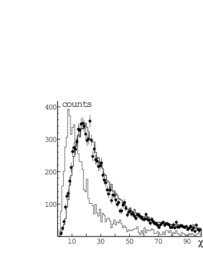
Figure 1: Distribution of $\chi^{2}$ for the tagged six-photon sample for data (points), MC background (solid line), and $10\,000$ events of MC signal (dashed line).

In the same plot, we also show the expected shape for signal events. Cutting at a reasonable $\chi^{2}$ value ($\chi^{2}/\rm{11}<3$) retains 71% of the signal while considerably reducing the background from false $K_{L}$-crash events (33%), in which the direction of the $K_{S}$ and $K_{L}$ are not correlated. However, this cut is not as effective on the 2S, 2A background, due to the soft energy spectrum of the fake clusters. In order to gain rejection power over the background for events with split and accidental clusters, we look at the correlation between the following two $\chi^{2}$-like estimators:

• $\zeta_{2}$, defined as

  $$\zeta_{2} = \frac{\Delta m_{1}^{2}}{\sigma_{m}^{2}}+\frac{\Delta m_{2}^{2}}{\sigma_{m}^{2}}+\frac{(E_{K_{S}}-\sum_{i}E_{\gamma_{i}})^{2}}{\sigma_{E}^{2}}+\frac{(P_{x}^{K_{S}}-\sum_{i}P_{x}^{\gamma_{i}})^{2}}{\sigma_{P_{x}}^{2}}+$$

  $$\;\;\;+\frac{(P_{y}^{K_{S}}-\sum_{i}P_{y}^{\gamma_{i}})^{2}}{\sigma_{P_{y}}^{2}}+\frac{(P_{z}^{K_{S}}-\sum_{i}P_{z}^{\gamma_{i}})^{2}}{\sigma_{P_{z}}^{2}}+\frac{(\pi-\vartheta_{\pi\pi}^{*})^{2}}{\sigma_{\vartheta_{\pi\pi}^{*}}^{2}}$$

  selecting the four out of six photons that provide the best kinematic agreement with the $K_{S}\rightarrow 2\pi^{0}$ decay hypothesis. This variable is quite insensitive to fake clusters. It is constructed using the two values of $\Delta m$ = $m_{i}-m_{\pi^{0}}$ (where $m_{i}$ is the invariant mass of a photon pair), the opening angle between $\pi^{0}$’s in the $K_{S}$ rest frame, and 4-momentum conservation. The resolutions on these quantities have been evaluated using a control sample of events with a $K_{L}$-crash and four prompt photons.

• $\zeta_{3}$, defined as

  $$\zeta_{3}=\frac{\Delta m_{1}^{2}}{\sigma_{m}^{2}}+\frac{\Delta m_{2}^{2}}{\sigma_{m}^{2}}+\frac{\Delta m_{3}^{2}}{\sigma_{m}^{2}}$$

  where the pairing of the six photons into $\pi^{0}$’s is performed by minimizing this variable. $\zeta_{3}$ is close to zero for a $K_{S}\rightarrow 3\pi^{0}$ event and large for six-photon background events.

For each estimator, the photon pairing with smallest $\zeta$ value is kept. Figure 2a shows the distribution of events in the $\zeta_{2}$-$\zeta_{3}$ plane for the MC background. Most of the events are concentrated at low values of $\zeta_{2}$,

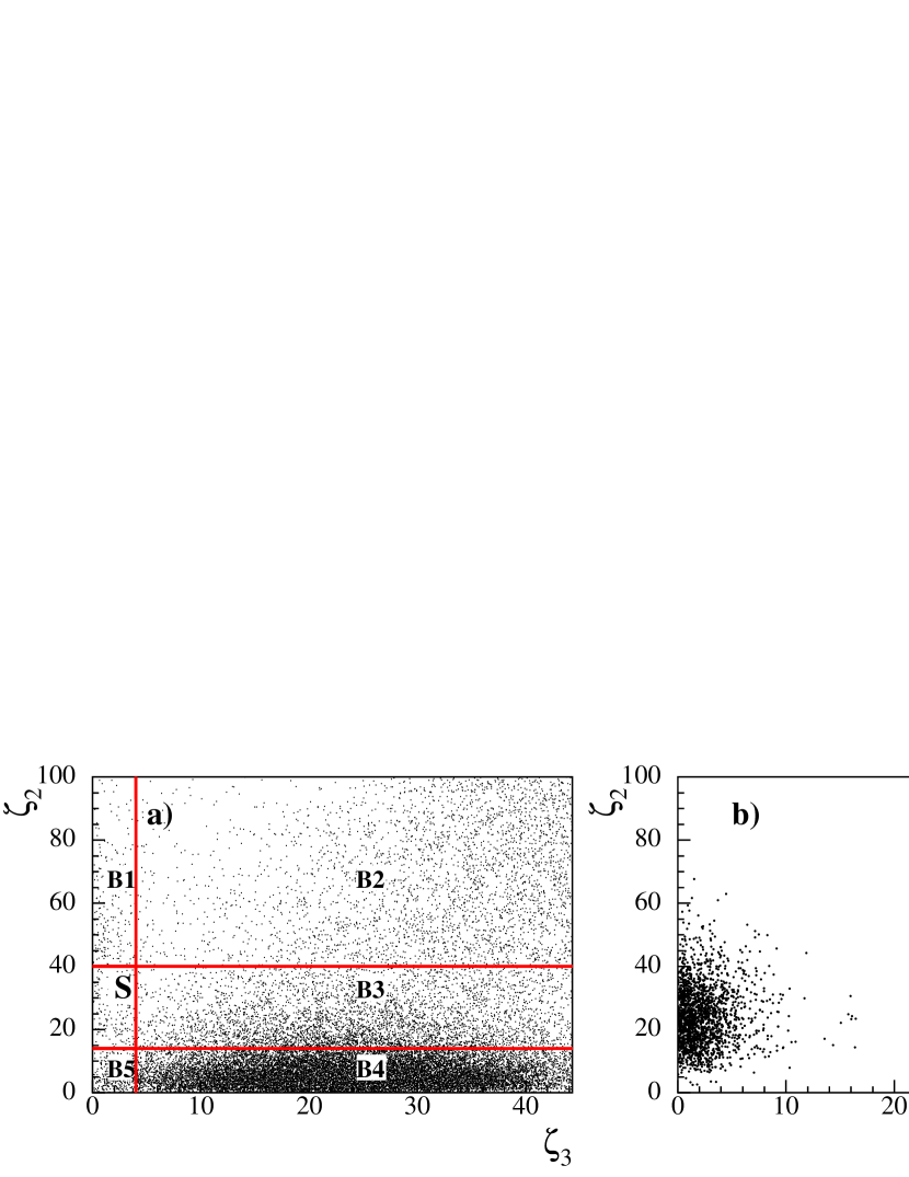
Figure 2: Scatter plot of $\zeta_{2}$ vs. $\zeta_{3}$ plane for the tagged six-photon sample: a) MC background, b) MC signal.

as expected for $K_{S}\rightarrow 2\pi^{0}$ events plus some additional isolated energy deposits in the EMC. A clear signal/background separation is achieved as can be seen by comparing the background and signal distributions in Figs. 2a and 2b.

Figure 3: Scatter plots of $\zeta_{2}$ vs. $\zeta_{3}$ for the tagged six-photon sample: data (a), MC sample with two split clusters (b), two accidental clusters (c), and false $K_{L}$-crash events (d).

We subdivide the $\zeta_{2}$-$\zeta_{3}$ plane into the six regions B1, B2, B3, B4, B5, and S as indicated in Fig. 2a. Region S, with the largest signal-to-background value, is the “signal” box.

	B1	B2	S	B3	B5	B4
data	$452\pm 21$	$10132\pm 101$	$282\pm 17$	$5037\pm 71$	$326\pm 18$	$22309\pm 149$
MC	$419\pm 19$	$9978\pm 104$	$282\pm 13$	$4816\pm 43$	$380\pm 10$	$22682\pm 190$

Table 3: Comparison between data and MC expectations in the different regions of the $\zeta_{2}$-$\zeta_{3}$ plane for the entire sample with a $K_{L}$-crash and six prompt photons. The boxes are defined as in Fig. 2a.

The scatter plot in the $\zeta_{2}$-$\zeta_{3}$ plane for the data is shown in Fig. 3a. Our MC simulation does not accurately reproduce the absolute number of 2S and 2A background events. This is also true of the predicted number of false $K_{L}$-crash events. However, the simulation does describe the kinematical properties of these events quite well. The two-dimensional $\zeta_{2}$-$\zeta_{3}$ distribution allows us to calibrate the contributions from the different backgrounds. The MC shapes for each of the three categories are shown in Figs. 3b-d. We perform a binned likelihood fit of a linear combination of these shapes to the data, excluding the signal-box region. From the fit we find the composition of the six-photon sample to be (37.9$\pm$1.0)%, (57.4$\pm$1.3)%, and (4.7$\pm$0.3)% for the 2S, 2A, and false $K_{L}$-crash categories, respectively.

As a check, we compare data and MC for the projected distribution in $\zeta_{3}$ for the three bands in $\zeta_{2}$, as shown in Figs. 4a-b. Excellent agreement is observed. The large peak at low values of $\zeta_{3}$ in the central band is due to the false $K_{L}$-crash events. As a final test, we compare data and MC in the signal box and the five surrounding control regions. The agreement is better than 10% in all regions, as seen from Table 3.

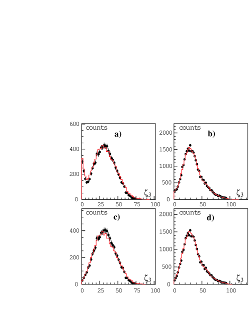
Figure 4: Distributions in $\zeta_{3}$ for the tagged six-photon sample. Plots on the left are for events in the central band in $\zeta_{2}$; plots on the right are for events in all other regions of the plane. The plots in the top row are for the entire sample, before any cuts are made. The plots in the bottom row are after the application of the track veto. In all cases, black points represent data; solid line represents MC.

Although cutting on $\chi^{2}$ substantially suppresses the false $K_{L}$-crash background, we reduce this background to a negligible level by vetoing events with tracks coming from the IP. This effectively eliminates events in which the false $K_{L}$-crash is due to a $K_{S}\rightarrow\pi^{+}\pi^{-}$ decay with the pion secondaries interacting in the quadrupoles. The effect on the signal region can be appreciated by comparison of Figs. 4a and 4c. Moreover, in order to improve the quality of the photon selection using $\zeta_{2}$, we cut on the variable $\Delta E=(m_{\phi}/2-\sum E_{i})/\sigma_{E}$, where $i$ = 1–4 stands for the four chosen photons in the $\zeta_{2}$ estimator and $\sigma_{E}$ is the appropriate resolution. For $K_{S}\rightarrow 2\pi^{0}$ decays plus two background clusters, we expect $\Delta E$ $\sim$ 0, while for $K_{S}\rightarrow\pi^{0}\pi^{0}\pi^{0}$, $\Delta E\geq m_{\pi^{0}}/\sigma_{E}$.

Before opening the signal box, we refine our cuts on $\chi^{2}$, $\zeta_{2}$, $\zeta_{3}$, and $\Delta E$ using the optimization procedure described in Ref. 13.

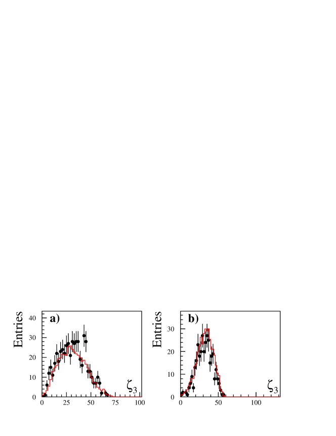
Figure 5: Distributions of $\zeta_{3}$ for the central band 12.1$<\zeta_{2}<$60 (a), the side-bands $\zeta_{2}<$12.1, $\zeta_{2}>$60 (b), after all cuts. Points represent data, solid line MC.

We end up choosing $\chi^{2}<40.4$ and $\Delta E>$1.7. The signal box is defined by 12.1 $<\zeta_{2}<$ 60 and $\zeta_{3}<$ 4.6.

Figures 5a and 5b show the $\zeta_{3}$ distributions for the central band and the sidebands in $\zeta_{2}$.

	B1	B2	S	B3	B4	B5
data	0	4 $\pm$ 2	2.0 $\pm$ 1.4	520 $\pm$ 23	3 $\pm$ 2	326 $\pm$ 18
MC	0	3.2 $\pm$ 0.8	3.1 $\pm$ 0.8	447 $\pm$ 10	2.5 $\pm$ 0.8	389 $\pm$ 10

Table 4: Same as Table 3, after all cuts.

In Table 4, we also list the number of events obtained in each of the six regions of the $\zeta_{2}$-$\zeta_{3}$ plane at this final stage of the analysis. In Figs. 6a-b we show the $\zeta_{2}$-$\zeta_{3}$ scatter plots for data and Monte Carlo.

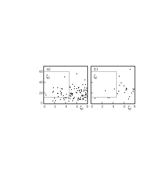
Figure 6: Distribution of $\zeta_{2}$ vs $\zeta_{3}$ after cuts: MC background 900 pb^-1 (a), data 450 pb^-1 (b).

The rectangular region illustrates the boundaries of the optimized signal box. Seventeen MC events are counted in this region before applying the data-MC scale factors resulting from the calibration procedure described above. Contributions to the scale factors include the fact that the simulated integrated luminosity is greater than that for the data set ($\times$2), the increased $K_{L}$-crash efficiency in the simulation ($\times$1.4), and the increased probability of having accidental or split clusters in the simulation (on average, $\sim$$\times$1.9).

The selection efficiency at each step of the analysis has been studied using the MC. After tagging, the efficiency for the six-photon selection is $(47.8\pm 0.1_{\rm{stat}})$%. Including all cuts, we estimate a total efficiency of $\epsilon_{3\pi}=(24.4\pm 0.1_{\rm{stat}}$)%. At the end of the analysis chain, we have two candidates with an expected background of $B^{\rm{exp}}=3.13\pm 0.82_{\rm{stat}}$.

In the same tagged sample, we also count events with photon multiplicities of three, four, or five. The corresponding efficiency is (91.8$\pm$0.2_stat)% for $K_{S}\rightarrow\pi^{0}\pi^{0}$ events. The residual background contamination is estimated to be (0.77 $\pm 0.24_{\rm{stat+sys}})\%$ and (0.65$\pm 0.10_{\rm{stat+sys}})\%$ in the 2001 and 2002 running periods respectively. Subtracting the background and correcting for the efficiency, we count $3.78\times 10^{7}$ $K_{S}\rightarrow\pi^{0}\pi^{0}$ events. We use this number to normalize the number of signal events when obtaining the branching ratio.

6 Systematic uncertainties

Systematics arise from uncertainties in estimation of the acceptance, backgrounds, and the analysis efficiency. The evaluation of the systematic uncertainties is described in detail in Ref. 14.

Concerning the acceptance of the event selection for both the 2$\pi^{0}$ and 3$\pi^{0}$ samples, we estimate the systematic errors in photon counting by comparing data and MC values for the $P_{A}$ and $P_{S}$ probabilities described above. The photon reconstruction efficiency for both data and MC is evaluated using a large sample of $\phi\rightarrow\pi^{+}\pi^{-}\pi^{0}$, $\pi^{0}$$\rightarrow$$\gamma$$\gamma$events. The momentum of one of the photons is estimated from tracking information and position of the other cluster. The candidate photon is searched for within a search cone. The efficiency is parameterized as a function of the photon energy. Systematics related to this correction are obtained from the variation of the efficiency as a function of the width of the search cone. The results are listed in Table 5 under the heading cluster.

	$\Delta\alpha/\alpha$ ($K_{S}\rightarrow 2\pi^{0}$)	$\Delta\alpha/\alpha$ ($K_{S}\rightarrow 3\pi^{0}$)
Cluster	0.16 %	0.70 %
Trigger	0.08 %	0.08 %
Background filter	0.20 %	0.08 %
Total	0.27 %	0.71 %

Table 5: Systematic acceptance uncertainties, $\Delta\alpha$, for the 2$\pi^{0}$ and 3$\pi^{0}$ event selection criteria.

The total uncertainty is smaller for the normalization sample since an inclusive selection criterion is used in this case.

The normalization sample also suffers a small ($0.4\%$) loss due to the use of a filter during data reconstruction to reject cosmic rays, Bhabha fragments from the low-beta quadrupole, and machine background events. This loss is estimated using the MC. We correct for it and add a 0.2% systematic error to the selection efficiency. The trigger and cosmic-ray veto efficiencies have been estimated with data for the normalization sample and extrapolated by MC to the signal sample. These efficiencies are very close to unity and the related systematics are negligible.

For the tagged six-photon sample, we have investigated the uncertainties related to the estimate of the background in the signal box after all cuts, $B^{\rm{exp}}$. We have first considered the error related to the calibration of the MC background composition by propagating the errors on the scale factors obtained from the fit. This corresponds to a relative error of $2.4\%$ on $B^{\rm{exp}}$. Moreover, we have investigated the extent to which the track-veto efficiency influences the residual false $K_{L}$-crash contamination. To do so, we examine the data-MC ratio, $R_{\beta}$, of the sidebands in $\beta^{*}$ for events rejected by this veto, since for true $K_{L}$’s $\beta^{*}$ peaks at $\sim$ 0.2 while false $K_{L}$-crashes are broadly distributed in $\beta^{*}$. We obtain $R_{\beta}=1.10\pm 0.01$. Knowing that in the MC only 24% of the fakes survive the veto, we find a fractional error of 32% on the fake background. Since false $K_{L}$-crash events account for 15% of the total background, the error on $B^{\rm{exp}}$ from data-MC differences in the track veto efficiency is 4.6%.

A control sample of $K_{S}\rightarrow 2\pi^{0}$ with four prompt photons has been used to compare the energy scale and resolution of the calorimeter in data and in the MC. The distributions of the $m$ and $\Delta E$ variables have also been compared by fitting them with Gaussians. By varying the mass and energy resolution by $\pm 1\sigma$ in the definitions of $\zeta_{2}$ and $\zeta_{3}$, we observe a relative change of 6.6% in the background estimate. Similarly, correcting for small differences in the energy scale for data and MC, we derive a systematic uncertainty of 6.7% on $B^{\rm{exp}}$.

Finally, we have tested the effect of the cut on $\chi^{2}$ by constructing the ratio between the cumulative distributions for data and MC. An error of 5% is obtained. A summary of all the systematic errors on the background estimate is given in Table 6.

	$\Delta B^{\rm{exp}}/B^{\rm{exp}}$	$\Delta\epsilon_{\rm ana}/\epsilon_{\rm ana}$
Background composition	2.4%	-
Track veto	4.8%	0.2%
Energy resolution	6.6%	0.5%
Energy scale	6.7%	1.0%
$\chi^{2}$	5.0%	1.8%
Total	11.5%	2.1%

Table 6: Systematic uncertainties on the expected background and analysis efficiency, $\epsilon_{\rm ana}$.

Adding in quadrature all sources we obtain a total systematic error of 12% on the background estimate.

To determine the systematics related to the analysis cuts for the signal, we have first evaluated the effect of the track veto. Using the MC signal sample, we estimate a vetoed event fraction of (3.7 $\pm$ 0.1)%. The data-MC ratio of the cumulative distributions for the track-vetoed events in the tagged six-photon sample is $R_{TV}=1.06\pm 0.03$, which translates into a 0.2% systematic error on the track-veto efficiency.

Because of the similarity of the $\chi^{2}$ distributions for the tagged four- and six-photon samples, as confirmed by MC studies, an estimate of the systematic error associated with the application of the $\chi^{2}$ cut can be obtained from the data-MC comparison of the cumulative $\chi^{2}$ distributions for the four-photon sample. The systematic error arising from data-MC discrepancies in the $\chi^{2}$ distribution is estimated to be 1.8% by this comparison.

Moreover, the efficiency changes related to differences between the calorimeter resolution and energy scale for data and MC events have been studied in a manner similar to that previously described for the evaluation of the systematics on the background. The systematic uncertainties on the analysis efficiency are summarized in Table 6. Adding all sources in quadrature we quote a total systematic error of 2.1% on the estimate of the analysis efficiency.

7 Results

At the end of the analysis, we find 2 events in the signal box with an estimated background of $B^{\rm{exp}}=3.13\pm 0.82_{\rm{stat}}\pm 0.37_{\rm{syst}}$. To derive an upper limit on the number of signal counts, we build the background probability distribution function, taking into account our finite MC statistics and the uncertainties on the MC calibration factors. This function is folded with a Gaussian of width equivalent to the entire systematic uncertainty on the background. Using the Neyman construction described in Ref. 15, we limit the number of $K_{S}\rightarrow 3\pi^{0}$ decays observed to 3.45 at 90% C.L., with a total reconstruction efficiency of $(24.36\pm 0.11_{\rm{stat}}\pm 0.57_{\rm{sys}})\%$. In the same tagged sample, we count $3.78\times 10^{7}$ $K_{S}\rightarrow\pi^{0}\pi^{0}$ events. This number is used for normalization. Finally, using the value BR($K_{S}\rightarrow\pi^{0}\pi^{0}$) = 0.3105 $\pm$ 0.0014 [16] we obtain:

$$\mbox{${\rm BR}$}(K_{S}\rightarrow 3\pi^{0})\leq 1.2\times 10^{-7}\;\;\;\;{\rm at}\;\;\;90\%\;\;\;{\rm C.L.},$$ (1)

which represents an improvement by a factor of $\sim$6 with respect to the best previous limit [4], and by a factor of 100 with respect to the best limit obtained with a direct search [2].

The limit on the BR can be directly translated into a limit on $|\eta_{000}|$:

 

$${|\eta_{000}|=}$$

  (2)

This result describes a circle of radius 0.018 centered at zero in the $\Re({\eta_{000}})$, $\Im{(\eta_{000})}$ plane and represents a limit $2.5$ times smaller than the result of Ref. 4. As follows from the discussion in that reference, our result confirms that the sensitivity of the $C$$P$$T$ test from unitarity is now limited by the uncertainty on $\eta_{+-}$.

References

- [1] G. D’Ambrosio et al., and measurements at DAΦNE, in The second DAΦNE handbook, L. Maiani et al. editors, Frascati, 63 (1995).
- [2] SND Collaboration, M. N. Achasov et al., Phys. Lett. B 459 (1999), 674.
- [3] CPLEAR Collaboration, A. Angelopoulos et al., Phys. Lett. B 425 (1998), 391.
- [4] NA48 Collaboration, A. Lai et al., Phys. Lett. B610 (2005), 165.
- [5] G.B. Thomson and Y. Zou, Phys. Rev. D 51 (1995), 1412.
- [6] KLOE Collaboration, M. Adinolfi et al., Nucl. Inst. Meth. A 488 (2002), 51.
- [7] KLOE Collaboration, M. Adinolfi et al., Nucl. Inst. Meth. A 482 (2002), 364.
- [8] KLOE Collaboration, M. Adinolfi et al., Nucl. Inst. Meth. A 483 (2002), 649.
- [9] KLOE Collaboration, M. Adinolfi et al., Nucl. Inst. Meth. A 492 (2002), 134.
- [10] S. Guiducci, Status Report on DAΦNE, in: P. Lucas, S. Weber (Eds.), Proceedings of the 2001 Particle Accelerator Conference, Chicago, IL., USA, 2001.
- [11] KLOE Collaboration, F. Ambrosino et al., Nucl. Inst. Meth. A 453 (2004), 403.
- [12] M. Martini and S. Miscetti, Determination of the probability of accidental coincidence between machine background and collision events and fragmentation of electromagnetic showers, KLOE note 201 (2005), http://www.lnf.infn.it/kloe.
- [13] J.F. Grivaz and F. Le Diberder, LAL 92-37 (1992).
- [14] M. Martini and S. Miscetti, A direct search for decay, KLOE note 200 (2005), http://www.lnf.infn.it/kloe.
- [15] G. J. Feldman and R. Cousins, Phys. Rev. D57 (1998), 57.
- [16] S. Eidelman et al., Phys. Lett. B 592 (2004).