Observation of Parity Violation in the $\Omega^{-}$ $\rightarrow$ $\Lambda$$K^{-}$ Decay

Abstract

The $\alpha$ decay parameter in the process $\Omega^{-}$ $\rightarrow$ $\Lambda$$K^{-}$ has been measured from a sample of 4.50 million unpolarized $\Omega^{-}$ decays recorded by the HyperCP (E871) experiment at Fermilab and found to be $[1.78{\pm}0.19({\rm stat}){\pm}0.16({\rm syst})]{\times}10^{-2}$. This is the first unambiguous evidence for a nonzero $\alpha$ decay parameter, and hence parity violation, in the $\Omega^{-}$ $\rightarrow$ $\Lambda$$K^{-}$ decay.
PACS: 11.30.Er, 13.30.Eg, 14.20.Jn
Keywords: Omega-minus decays; Parity violation; Alpha decay parameter

, , , , , , , , , , , , , , , , , , , , , , , , , , , , ,

HyperCP Collaboration

Our knowledge of the $\Omega^{-}$ hyperon and its decays remains incomplete, despite its long and illustrious role in particle physics. Its spin and parity have not been firmly established, and it alone among the hyperons has yet to exhibit parity violation in its two-body weak decays. The Particle Data Group (PDG) values of the $\alpha$ decay parameters of the three such decays, $\Omega^{-}$ $\rightarrow$ $\Lambda$$K^{-}$, $\Omega^{-}$ $\rightarrow$ $\Xi^{-}$$\pi^{0}$, and $\Omega^{-}$ $\rightarrow$ $\Xi^{0}$$\pi^{-}$, respectively $-0.026{\pm}0.023$, $+0.05{\pm}0.21$, and $+0.09{\pm}0.14$ [2], are consistent with zero, where $\alpha$ is a measure of the interference between the $P$- and $D$-wave final-state amplitudes:

$$\alpha=\frac{2{\rm Re}(P^{\ast}D)}{|P|^{2}+|D|^{2}}.$$ (1)

A nonzero value of $\alpha$ is manifest evidence of parity violation. In contrast, all other hyperons have been shown to have nonzero $\alpha$ decay parameters. The smallest are those of the $\Sigma^{+}$ $\rightarrow$ n$\pi^{+}$ and the $\Sigma^{-}$ $\rightarrow$ n$\pi^{-}$ decays, both of which are 0.068; the largest is almost unity: $\alpha=-0.980$ in $\Sigma^{+}$ $\rightarrow$ $p$$\pi^{0}$ decays [2]. The two-body nonleptonic $\Omega^{-}$ decays are expected to be nearly parity conserving [3], and hence predominantly $P$ wave, implying a small $\alpha$ decay parameter, which is consistent with the experimental results.

Recently, we have reported evidence of parity violation in an analysis of 0.96 million $\Omega^{-}$ $\rightarrow$ $\Lambda$$K^{-}$ decays taken in the 1997 Fermilab fixed-target running period, yielding $\makebox{$\alpha_{\Omega}$}=[2.07{\pm}0.51({\rm stat}){\pm}0.81({\rm syst})]{\times}10^{-2}$ [4]. (Throughout this Letter $\alpha_{\Omega}$ will refer only to the $\Lambda$$K^{-}$ decay mode of the $\Omega^{-}$.) We report here another measurement of $\alpha_{\Omega}$ using 4.50 million events taken during the 1999 Fermilab fixed-target running period.

The experiment was mounted in the Meson Center beam line at Fermilab using an apparatus [5] built to search for CP violation in hyperon decays (see Fig. 1).

Figure 1: Plan view of the HyperCP spectrometer.

A negatively charged secondary beam with an average momentum of 160 GeV/$c$ was produced by steering an 800 GeV/$c$ proton beam onto a 60 mm long, $2{\times}2$ mm² wide, Cu target. The target was followed by a curved collimator embedded in a dipole magnet (“Hyperon Magnet”). The $\Omega^{-}$’s were produced at an average angle of $0^{\circ}$, ensuring that their polarization was zero. The secondary beam exited the collimator upward at 19.51 mrad relative to the incident proton beam direction. A 13 m long evacuated pipe (“Vacuum Decay Region”) immediately followed the collimator exit. After the Vacuum Decay Region was a high-rate magnetic spectrometer employing nine multiwire proportional chambers (MWPCs), four in front of a pair of dipole magnets (“Analyzing Magnets”), and five behind. Particles with the same sign as the secondary beam were deflected by the Analyzing Magnets to the beam-left side of the apparatus, and those with the opposite sign to beam-right. The highly redundant tracking system facilitated very high track-reconstruction efficiencies. The trigger required the coincidence of at least one hit counter in each of the Same-Sign (SS) and Opposite-Sign (OS) hodoscopes situated on either side of the secondary beam (the LR subtrigger), along with an energy deposit of at least ${\approx}40$ GeV in the hadronic calorimeter. This energy threshold was well below the 60 GeV of the lowest-energy protons from $\Omega^{-}$ decays, all of which entered the calorimeter, and above the energy where the calorimeter efficiency plateaued at ${\approx}99$%. Since there was a high probability that both the $K^{-}$ and the $\pi^{-}$ would hit the SS hodoscope and since the OS hodoscope had two layers of counters, the efficiency of the LR subtrigger was extremely high (${\approx}$99.5%). Events that satisfied the trigger were written to magnetic tape by a high-rate data acquisition system [6].

The analysis reported here is from data taken with the negative-polarity secondary beam. The 29 billion recorded events were initially reconstructed and separated according to event type using loose event-selection cuts. This left a total of 56 million candidate events. The raw event information was preserved at this (as well as every subsequent) stage. Final event-selection criteria were applied after careful study and were tuned to maximize the signal-to-background ratio. The most important requirements were that: (1) the $\chi^{2}/{\rm df}$ for a geometric fit to the decay topology be less than 2.5; (2) the distance-of-closest-approach for the tracks forming the $\Lambda$ and $\Omega^{-}$ decay vertices be less than 4 mm; (3) the $x$ and $y$ separations from the target center of the extrapolated $\Omega^{-}$ trajectory satisfy the inequality $(x/2.0\,{\rm mm})^{2}+(y/2.2\,{\rm mm})^{2}\leq 1.0$; (4) both the $\Omega^{-}$ and the $\Lambda$ decay vertices lie at least 0.28 m (0.32 m) downstream (upstream) of the entrance (exit) of the Vacuum Decay Region, and that the $\Omega^{-}$ vertex precede that of the $\Lambda$; (5) the $p$$\pi^{-}$$\pi^{-}$ ($\pi^{+}$$\pi^{-}$$\pi^{-}$) invariant mass be greater than 1.355 GeV/$c^{2}$ (0.520 GeV/$c^{2}$), in order to eliminate $\Xi^{-}$ $\rightarrow$ $\Lambda$$\pi^{-}$ $\rightarrow$ $p$$\pi^{-}$$\pi^{-}$ ($K^{-}$ $\rightarrow$ $\pi^{+}$$\pi^{-}$$\pi^{-}$) decays; (6) the $p$$\pi^{-}$ and $p$$\pi^{-}$$K^{-}$ invariant masses be respectively within ${\pm}4.0$ MeV/$c^{2}$ ($4.3\,\sigma$) and ${\pm}8.0$ MeV/$c^{2}$ ($5.0\,\sigma$) of the true $\Lambda$ and $\Omega^{-}$ masses; and (7) no particle have momentum less than 12 GeV/$c$. After all these cuts the number of events remaining was 4.735 million. Monte Carlo simulation indicated that 55.3% of $\Omega^{-}$ $\rightarrow$ $\Lambda$$K^{-}$ $\rightarrow$ $p$$\pi^{-}$$K^{-}$ decays for which the $\Omega^{-}$ exited the collimator passed these cuts. The cuts that eliminated the greatest numbers of signal events were the $p$$\pi^{-}$$\pi^{-}$ invariant mass and the $\Omega^{-}$ vertex requirements.

Figure 2 shows the $p$$\pi^{-}$$K^{-}$ and $p$$\pi^{-}$ invariant-mass distributions after event selection cuts. The background-to-signal ratio, determined using a double-Gaussian plus second-degree polynomial fit to the invariant-mass distribution, is $(0.33{\pm}0.03)$% in the region within ${\pm}5.0\,\sigma$ of the $\Omega^{-}$ mass. The background under the $p$$\pi^{-}$ mass peak is less than half this. Dominant backgrounds were misreconstructed $\Xi^{-}$ $\rightarrow$ $\Lambda$$\pi^{-}$ $\rightarrow$ $p$$\pi^{-}$$\pi^{-}$ decays and $\Omega^{-}$ $\rightarrow$ $\Xi^{0}$$\pi^{-}$ $\rightarrow$ $\Lambda$$\pi^{0}$$\pi^{-}$ $\rightarrow$ 
$p$$\pi^{-}$$\pi^{-}$$\gamma$$\gamma$ decays.

Figure 2: The $p$$\pi^{-}$$K^{-}$ (left) and $p$$\pi^{-}$ (right) invariant-mass distributions, after all cuts except the respective mass cuts. Arrows delimit the accepted mass regions.

The $\Omega^{-}$ alpha parameter was measured through the asymmetry in the $\Lambda$ $\rightarrow$ $p$$\pi^{-}$ decay distribution. In the decay of an unpolarized $\Omega^{-}$ to a $\Lambda$ and a $K^{-}$, the $\Lambda$ is produced in a helicity state with its helicity given by $\alpha_{\Omega}$ [7]. Hence the decay distribution of the proton in that $\Lambda$ rest frame in which the $\Lambda$ direction in the $\Omega^{-}$ rest frame defines the polar axis — the Lambda Helicity Frame shown in Fig. 3 — is given by

$$\frac{dN}{d\cos\theta}=\frac{N_{0}}{2}(1+\makebox{$\alpha_{\Omega}$}\makebox{$\alpha_{\Lambda}$}\cos\theta),$$ (2)

where $\theta$ is the polar angle of the proton and $\alpha_{\Lambda}$ is the alpha decay parameter in $\Lambda$ $\rightarrow$ $p$$\pi^{-}$.

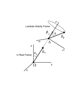
Figure 3: The Lambda Helicity Frame.

Since the $\Lambda$ decay direction in the $\Omega^{-}$ rest frame changes from event to event, so too does the polar axis of the Lambda Helicity Frame along which the $\Lambda$ polarization must lie: knowledge of the direction of the putative $\Lambda$ polarization is of enormous importance as it greatly minimizes biases. The analysis “locks in” to the changing direction of the $\Lambda$ polarization. Biases, on the other hand, such as uncorrected detector inefficiencies, are fixed in the laboratory frame. Hence the Lambda Helicity Frame analysis acts much like a lock-in amplifier, except that it locks into a known direction rather than a known frequency.

The proton $\cos\theta$ acceptance was measured and corrected for using a hybrid Monte Carlo (HMC) technique that has been used in many similar such measurements [8]. Monte Carlo events were generated by taking all parameters from real events except the proton and pion direction in the rest frame of the $\Lambda$. An isotropic $\Lambda$ $\rightarrow$ $p$$\pi^{-}$ decay was generated, and the proton and pion were boosted back into the laboratory frame using the real $\Lambda$ momentum. Their trajectories were then traced through the apparatus, with the detector responses simulated where appropriate (using measured efficiencies), and all MWPC wire hits not associated with the real proton and pion tracks kept. The simulation included multiple scattering and slope-dependent multiple-wire hit probabilities which were tuned to match data. The HMC simulated the data extremely well, as is evident by the small $\chi^{2}/{\rm df}$ in the matching of the real and HMC proton distributions in the Lambda Helicity Frame (see discussion below). Real and HMC distributions of proton and pion tracks at various places along the spectrometer also showed excellent agreement. The HMC proton and pion tracks, in conjunction with the real kaon, were required to satisfy the trigger requirements, and were reconstructed by the standard track-finding program, with the same cuts applied to all parameters formed from them that were applied to the real events. Ten accepted HMC events were used for each real event. If over 300 generated HMC events were required to get the ten, then both the real and associated HMC events were discarded; this eliminated regions of low acceptance and reduced the computer time needed for the analysis. It eliminated 4.9% of the events. Increasing the upper limit beyond 300 events had no effect on the result.

Since the HMC events were generated with a uniform proton $\cos\theta$ distribution, each accepted HMC event was then weighted by

$$W=\frac{1+S\cos\theta_{f}}{1+S\cos\theta_{r}},$$ (3)

where $S$ is the slope (to be determined) of the proton $\cos\theta$ distribution and $\theta_{f}$ and $\theta_{r}$ are, respectively, the HMC (“fake”) and real proton polar angles in the Lambda Helicity Frame. Note that in the absence of a background correction $S=\makebox{$\alpha_{\Omega}$}\makebox{$\alpha_{\Lambda}$}$. The numerator in Eq. (3) in effect polarizes the HMC sample, while the denominator removes the polarization bias accrued from using parameters from real polarized $\Lambda$ decays. To facilitate handling the unknown slope $S$, the weights, binned in $\cos\theta_{f}$, were approximated by the polynomial series expansion

$$W\approx(1+S\cos\theta_{f})[1-S\cos\theta_{r}+(S\cos\theta_{r})^{2}-\cdots+(S\cos\theta_{r})^{10}].$$ (4)

The polynomial coefficients, which depend only on $\cos\theta_{f}$ and $\cos\theta_{r}$, were summed, and then $S$ was extracted by minimizing the $\chi^{2}$ difference between the real and weighted HMC proton $\cos\theta$ distributions. The error was determined by finding the variation in $S$ needed to increase $\chi^{2}$ by one. It includes the uncertainty in the acceptance as determined by the HMC events.

The analysis procedure was extensively checked by Monte Carlo simulation. Monte Carlo $\Omega^{-}$ $\rightarrow$ $\Lambda$$K^{-}$ $\rightarrow$ $p$$\pi^{-}$$K^{-}$ events were simulated using the real hodoscope, MWPC, and calorimeter efficiencies, and required to pass the same cuts as the real data. These were analyzed by the HMC analysis code. The input and extracted values of $\alpha_{\Omega}$$\alpha_{\Lambda}$ were found to be consistent over a wide range of $\alpha_{\Omega}$ input values, with an average difference of $(0.017{\pm}0.042){\times}10^{-2}$. As a cross-check, 78 000 $\Xi^{-}$ $\rightarrow$ $\Lambda$$\pi^{-}$ $\rightarrow$ $p$$\pi^{-}$$\pi^{-}$ decays available from the same dataset were analyzed using exactly the same analysis program, with selection criteria tuned for the $\Xi^{-}$ decay. The fit to the proton $\cos\theta$ distribution was good, with $\chi^{2}/{\rm df}=14/19$. The correct sign of $\alpha_{\Xi}$$\alpha_{\Lambda}$ was found, which is opposite the sign of our value of $\alpha_{\Omega}$$\alpha_{\Lambda}$, and the magnitudes of the measured and PDG values of $\alpha_{\Xi}$$\alpha_{\Lambda}$ were consistent within the statistical errors.

Figure 4: The real (lines) and weighted HMC (points) proton $\cos\theta$ distributions. The total number of HMC events has been scaled down by a factor of 10.

A total of 4 504 896 real events were analyzed by the method described above. The real and weighted HMC proton $\cos\theta$ distributions are shown in Fig. 4, and the differences between the real and HMC proton $\cos\theta$ distributions, weighted and unweighted, are shown in Fig. 5. The nonisotropic nature of the real proton $\cos\theta$ distribution, compared to the isotropically generated HMC distribution, is clear from the top plot of Fig. 5. It is unambiguous evidence of a nonzero $\alpha$ decay parameter. The bottom plot shows the same comparison, except that the HMC events have been weighted by the best-fit value of $S$. The extracted slope of the proton $\cos\theta$ distribution is $S=(1.16{\pm}0.12){\times}10^{-2}$ with $\chi^{2}/{\rm df}=23/19$, where the error is statistical.

Figure 5: The relative differences between the real (N_r) and HMC (N_f) proton $\cos\theta$ distributions for unweighted (top) and weighted (bottom) HMC events. The total number of HMC events has been scaled down by a factor of 10.

To extract $\alpha_{\Omega}$$\alpha_{\Lambda}$ from the proton $\cos\theta$ slope, the small background contribution to $S$ was subtracted. To estimate the proton $\cos\theta$ slope from the background events the same analysis procedure was performed on five sideband regions, three below and two above the $\Omega^{-}$ mass region. The average sideband proton $\cos\theta$ slope was found to be $S_{\rm sb}=(7.2{\pm}3.0){\times}10^{-2}$, with average $\chi^{2}/{\rm df}=19/19$. No mass dependence of $S_{\rm sb}$ was apparent. The contribution to $S$ of the background under the mass peak was corrected for by subtracting the appropriate fraction of $S_{\rm sb}$ from $S$, giving $\makebox{$\alpha_{\Omega}$}\makebox{$\alpha_{\Lambda}$}=[1.14{\pm}0.12({\rm stat})]{\times}10^{-2}$. Note that this correction is only a 1.7% effect.

Figure 6: The value of $\alpha_{\Omega}$$\alpha_{\Lambda}$ vs. the $\Omega^{-}$ momentum.

The stability of the result was studied as a function of several parameters. The value of $\alpha_{\Omega}$$\alpha_{\Lambda}$ was independent of the $\Omega^{-}$ momentum, as shown in Fig. 6, and there was no dependence on the $z$ location of the $\Omega^{-}$ decay vertex. The non-background-subtracted slope $S$, measured on a run-by-run basis for all 175 runs in the dataset, shows no evidence of a temporal dependence (see Fig. 7).

Figure 7: Run-by-run values of the proton slope $S$. The dashed line represents the best-fit value.

Systematic errors were small because of the high efficiencies of the spectrometer elements and because of the power of the Lambda Helicity Frame analysis. The dominant systematic errors are listed in Table 1. The effects of uncertainties in detector inefficiencies — MWPCs, trigger hodoscopes, and hadronic calorimeter — on $\alpha_{\Omega}$$\alpha_{\Lambda}$ were found to be negligible. No statistically significant difference in $S$ was found between using perfect and measured detector efficiencies when simulating the HMC proton and pion. The combined effect of the uncertainties in the fields of the Analyzing Magnets, 5.5 G, was also negligible. A small fraction of the daughter $\pi^{-}$’s and $K^{-}$’s decayed before exiting the apparatus. (Approximately 0.7% of the $\pi^{-}$’s decayed before the last MWPC.) The effect of such decays on $\alpha_{\Omega}$$\alpha_{\Lambda}$ was studied using Monte Carlo events and data and found to be negligible. The error in the background subtraction was estimated by assuming that the error in the average sideband slope $S_{\rm sb}$ was equal to the average sideband slope, ${\delta}S_{\rm sb}=7.2{\times}10^{-2}$, and using a 25% error in the background-to-signal ratio, both very conservative assumptions. It too is negligible.

Table 1: Systematic errors.

Source                             Error ($10^{-2}$)
Event selection cut variations	0.	088
Validation of analysis code	0.	042
Background subtraction uncertainty	0.	024
Detector inefficiency uncertainties	0.	010
Analyzing Magnets field uncertainties	0.	006

The largest systematic uncertainty was the sensitivity of the measurement to the values of the cuts used to define the data sample. The most important were the cuts on the $p$$\pi^{-}$ and $p$$\pi^{-}$$K^{-}$ invariant masses and, less importantly, the 12 GeV/$c$ minimum momentum cut. The effect of changes in these cut values was $0.088{\times}10^{-2}$. The total systematic error, including the upper limit in the uncertainty of the MC validation of the analysis program ($0.042{\times}10^{-2}$), is $0.10{\times}10^{-2}$. This is a factor of five reduction in the systematic error of $0.52{\times}10^{-2}$ reported in the analysis of the 1997 data [4]; most of the improvement comes from incorporating the measured detector and track-finding inefficiencies into the HMC simulation in this analysis.

To summarize, we find from a sample of 4 504 896 $\Omega^{-}$ $\rightarrow$ $\Lambda$$K^{-}$ $\rightarrow$ $p$$\pi^{-}$$K^{-}$ decays the value $\makebox{$\alpha_{\Omega}$}\makebox{$\alpha_{\Lambda}$}=[1.14{\pm}0.12({\rm stat}){\pm}0.10({\rm syst})]{\times}10^{-2}$. Using $\makebox{$\alpha_{\Lambda}$}=0.642{\pm}0.013$ [2], $\alpha_{\Omega}$ is found to be $[1.78{\pm}0.19({\rm stat}){\pm}0.16({\rm syst})]{\times}10^{-2}$, where the contribution of the uncertainty in the value of $\alpha_{\Lambda}$ to the systematic error is negligible. Our measurement represents a factor of nine improvement in precision over the current PDG value. It is $1.9\,\sigma$ from the PDG average of $(-2.6{\pm}2.3){\times}10^{-2}$, and opposite in sign. This measurement is consistent with the recent result we reported [4] from an independent analysis of data taken in the 1997 fixed-target running period, but with a factor of four smaller error. With a magnitude that is 7.2 $\sigma$ from zero, it represents unambiguous evidence of parity violation in the $\Omega^{-}$ $\rightarrow$ $\Lambda$$K^{-}$ decay. As predicted, $\alpha_{\Omega}$ is small; indeed it is the smallest of all the $\alpha$ parameters that have been measured in the two-body weak decays of hyperons.

References

-
[1]
M. Baubillier et al., Phys. Lett. B 78 (1978) 342;
M. Deutschmann et al., Phys. Lett. B 73 (1978) 96. - [2] S. Eidelman et al. (Particle Data Group), Phys. Lett. B 592 (2004) 1.
-
[3]
M. Suzuki, Prog. Theor. Phys. 32 (1964) 138;
Y. Hara, Phys. Rev. 150 (1966) 1175;
J. Finjord, Phys. Lett. B 76 (1978) 116. - [4] Y. Chen et al., Phys. Rev. D 71 (2005) 051102(R).
- [5] R.A. Burnstein et al., Nucl. Instrum. Methods A 541 (2005) 516.
-
[6]
C.G. White et al., Nucl. Instrum. Methods A 474 (2001) 67;
C.G. White et al., IEEE Trans. Nucl. Sci. 49 (2002) 568. -
[7]
K.B. Luk, Ph.D. thesis, Rutgers University, 1983;
J. Kim, J. Lee, J.S. Shim, and H.S. Song, Phys. Rev. D 46 (1992) 1060. - [8] G. Bunce, Nucl. Instrum. Methods, 172 (1980) 553.