A Search for New Physics with High Mass Tau Pairs in Proton–Antiproton Collisions at $\bf\sqrt{\rm s}$ = 1.96 TeV at CDF

Abstract

We present the results of a search for new particles decaying to tau pairs using the data corresponding to an integrated luminosity of 195 pb^-1 collected from March 2002 to September 2003 with the CDF detector at the Tevatron. Hypothetical particles, such as $Z^{\prime}$ and MSSM Higgs bosons can potentially produce the tau pair final state. We discuss the method of tau identification, and show the signal acceptance versus new particle mass. The low-mass region, dominated by $Z\to\tau\tau$, is used as a control region. In the high-mass region, we expect $2.8\pm 0.5$ events from known background sources, and observe $4$ events in the data sample. Thus no significant excess is observed, and we set upper limits on the cross section times branching ratio as a function of the masses of heavy scalar and vector particles.

© 2005
Zongru Wan
ALL RIGHTS RESERVED

Table of Contents

toc

List of Tables

1. 2.1 Leptons and quarks in the SM
2. 2.2 Force carriers in the SM
3. 2.3 Quantum numbers of the fermions
4. 2.4 Couplings to fermions in the SM
5. 4.1 Tau dominant decay modes
6. 4.2 Tau pair final states
7. 5.1 Tau identification cuts
8. 5.2 Tau identification efficiency measurement
9. 5.3 Jet$\to\tau$ misidentification rate measurement
10. 5.4 Estimate $W\to\tau\nu$ events
11. 5.5 Expected and observed $W\to\tau\nu$ events
12. 5.6 Electron identification cuts
13. 5.7 Electron identification efficiency measurement
14. 5.8 Muon identification cuts
15. 5.9 Muon identification efficiency measurement in data
16. 5.10 Muon identification efficiency measurement in MC
17. 5.11 Muon reconstruction efficiency measurement in data
18. 5.12 Muon reconstruction efficiency measurement in MC
19. 5.13 The uncertainty in acceptance due to instrumental $\,/\!\!\!\!E_{T}$
20. 6.1 Event kinematic cuts
21. 7.1 Drell-Yan background estimates in the control region
22. 7.2 Fake background estimates in the control region
23. 7.3 Systematic uncertainties on fake backgrounds in the control region
24. 7.4 Expected and observed events in the control region
25. 8.1 $Z^{\prime}\to\tau\tau$ signal acceptance
26. 8.2 $A\to\tau\tau$ signal acceptance
27. 8.3 Drell-Yan background estimates in the signal region
28. 8.4 Fake background estimates in the signal region
29. 8.5 Systematic uncertainties on fake backgrounds in the signal region
30. 8.6 PDF uncertainty
31. 8.7 Systematic uncertainties and the affected channels
32. 8.8 Uncertainties of $Z^{\prime}\to\tau\tau$ signal acceptance
33. 8.9 Uncertainties of $A\to\tau\tau$ signal acceptance
34. 8.10 Uncertainties of backgrounds in the signal region
35. 9.1 Expected and observed events in the signal region
36. 9.2 The 95% CL upper limits

List of Figures

1. 1.1 Run I high-mass di-tau candidate event
2. 2.1 SU(3)_C$\times$SU(2)_L$\times$U(1)_Y gauge symmetries
3. 2.2 Particles in the Supersymmetry Theory
4. 2.3 Tau pair production $p\bar{p}\to\gamma^{*}/Z\to\tau\tau$ in the SM
5. 2.5 Tree-level Feynman diagrams for $Z^{\prime}\to\tau\tau$ and $A\to\tau\tau$
6. 3.1 Aerial view of Fermilab
7. 3.3 $p\bar{p}$ collision
8. 3.4 Run II instantaneous initial luminosity
9. 3.6 Solid cutaway view of CDF II detector
10. 3.8 CDF II tracking volume
11. 3.2.2 Tracking
12. 3.11 Calorimeter tower segmentation in $\eta-\phi$ space
13. 3.2.3 Calorimetry
14. 3.16 Muon stub matching to a track
15. 3.17 Muon coverage in $\eta$ and $\phi$
16. 3.18 Trigger system block diagram
17. 3.19 Average number of interactions per crossing
18. 3.20 Data flow of “deadtimeless” trigger and data acquisition
19. 5.1 Particle identification and missing transverse energy
20. 5.2 Illustration of tau isolation cone definitions
21. 5.3 Lack of geometry invariance in $\Delta R$ cone
22. 5.4 Tau “shrinking” signal cone as a function of energy
23. 5.5 Tau track/$\pi^{0}$ “shrinking” signal cone
24. 5.6 Electron removal in tau identification
25. 5.7 EM calorimeter isolation in tau identification
26. 5.8 Tau identification efficiency vs. energy
27. 5.9 Jet$\to\tau$ misidentification rate vs. energy
28. 5.10 Discrepancies of jet$\to\tau$ misidentification rates
29. 5.11 Jet cluster: mass vs. energy, and boost vs. energy
30. 5.13 Jet$\to\tau$ misidentification rate vs. energy, in boost slices
31. 5.14 Demonstration of estimating jet$\to\tau$ misidentification
32. 5.15 Lepton in data and in MC, and lepton data/MC scale factors
33. 5.16 Offline luminosity and L3 cross section of the TAU_MET trigger
34. 5.17 Number of jets in $Z\to\mu\mu$ data and MC
35. 5.19 Distributions of tau variables using $W\to\tau\nu$ events
36. 5.20 $\Upsilon\to ee$ in data
37. 5.22 $\Upsilon\to\mu\mu$ for CMUP muon identification efficiency measurement
38. 5.24 $\Upsilon\to\mu\mu$ for CMX muon identification efficiency measurement
39. 5.26 $\Upsilon\to\mu\mu$ for CMUP muon reconstruction efficiency measurement
40. 5.28 $\Upsilon\to\mu\mu$ for CMX muon reconstruction efficiency measurement
41. 5.30 Instrumental $\,/\!\!\!\!E_{T}$ in data and MC
42. 6.1 L1 $\,/\!\!\!\!E_{T}>$ 25 GeV trigger efficiency vs. offline $\,/\!\!\!\!E_{T}$ for di-tau event
43. 7.1 Drell-Yan mass spectra in different mass regions
44. 7.2 Cross check fake background estimate
45. 7.3 Distributions of the $\tau_{e}\tau_{h}$ channel in the control region
46. 7.4 Distributions of the $\tau_{\mu}\tau_{h}$ channel in the control region
47. 7.5 Distributions of the $\tau_{h}\tau_{h}$ channel in the control region
48. 8.1 Signal acceptance of $Z^{\prime}\to\tau\tau$
49. 9.1 Distribution of visible mass in the signal and control regions
50. 9.2 $\tau_{e}\tau_{h}$ candidate run=152669 event=629080 $m_{vis}$=148 GeV/$c^{2}$
51. 9.3 $\tau_{e}\tau_{h}$ candidate run=153693 event=815662 $m_{vis}$=129 GeV/$c^{2}$
52. 9.4 $\tau_{e}\tau_{h}$ candidate run=160591 event=207616 $m_{vis}$=125 GeV/$c^{2}$
53. 9.5 $\tau_{e}\tau_{h}$ candidate run=162252 event=612118 $m_{vis}$=124 GeV/$c^{2}$
54. 9.6 Upper limits at 95% CL for vector and scalar bosons
55. 9.7 Exclusion region for $Z^{\prime}$
56. B.1 Global and local transformations
57. B.2 Spontaneous symmetry breaking of Higgs potential
58. C.1 Proton’s parton density functions
59. D.1 Boost two-body decay from rest frame to lab frame
60. D.2 Separation angle vs. boost, calculated in $\theta^{*}$ slices

Chapter 1 Introduction

The Standard Model (SM) combines the electroweak theory together with Quantum Chromodynamics (QCD) of strong interactions and shows good agreement with collider experiments. However the SM does not include gravity and is expected to be an effective low-energy theory.

The Fermilab Tevatron is currently the high energy frontier of particle physics and delivers proton-antiproton collisions at high luminosity.

The Run II of the Collider Dectector at Fermilab (CDF) continues the precision measurements of hadron collider physics and the search for new physics at and above the electroweak scale. With the precision capability at the energy frontier, we can attack the open questions of high energy physics from many complementary directions, including: the properties of top quark, the precision electroweak measurements, e.g. mass of the $W$ boson, the direct searches for new phenomena, the tests of perturbative QCD at Next-to-Leading-Order and large $Q^{2}$, and the constraint of the CKM matrix with high statistics of the B decays.

This thesis is about a direct search for new particles decaying to tau pairs. The evidence for such new particles is that at accessible energies the events with tau pairs deviate clearly and significantly from the SM prediction.

In Run I CDF recorded an unusual event in which there were two very high energy $\tau\to h\nu$ candidates nearly back-to-back in direction. Figure 1.1 shows a display of the event. This event was recorded in the data sample from the missing transverse energy trigger, and was noticed in the context of the Run I charged Higgs search [1]. In Run I, a posteriori, it was not possible to estimate a probability for observing such an event, though less than about 0.1 such events were expected from backgrounds, including $Z/\gamma^{*}\to\tau\tau$ Drell-Yan ($q\bar{q}\to Z/\gamma^{*}\to l^{+}l^{-}$).

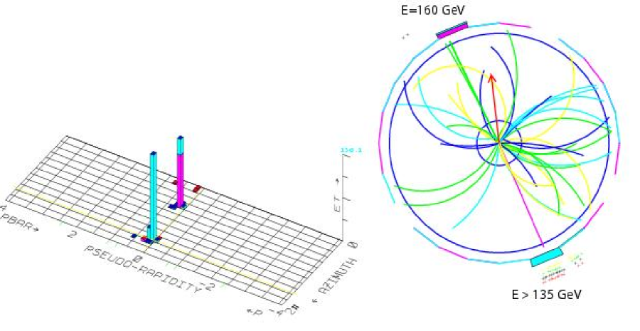
Figure 1.1: Run I high-mass di-tau candidate event. The left plot shows energy measurement in calorimeters and the event is very clean. The right plot shows the display in the transverse plane. The three-prong identified tau object has energy 160 GeV. The one-prong identified tau object has energy at least 135 GeV. There is also a significant missing transverse energy indicating significant neutrinos. The scale of the invariant mass of the two tau objects and the neutrinos is above 300 GeV/$c^{2}$.

Various new physics processes can lead to very high-mass tau pairs, for example, the new vector boson $Z^{\prime}\to\tau\tau$ predicted in the extension to the Standard Model by adding a new U(1) gauge symmetry and the pseudoscalar Higgs boson $A\to\tau\tau$ predicted in the minimum supersymmetric extension of the Standard Model (MSSM). The known backgrounds are from the high-mass tail of Drell-Yan processes (mainly $Z/\gamma^{*}\to\tau\tau$) as well as jet$\to\tau$ fakes from $W$+jets, QCD di-jet, and mutli-jet events.

In this analysis we search for such signal processes by performing a counting experiment. We select events with $e+\tau_{h}$, $\mu+\tau_{h}$, and $\tau_{h}+\tau_{h}$ (here, “$\tau_{h}$” means a $\tau$ hadronic decay). We construct an invariant mass which we call $m_{vis}$ using the four-vector sum of the lepton, the tau, and the missing transverse energy vector (ignoring in the latter the $z$ component). The region which has $m_{vis}>120$ GeV/$c^{2}$ is defined as the signal region, while the region which has $m_{vis}<120$ GeV/$c^{2}$ is retained as a control region. We perform a blind analysis in the signal region, i.e., we do not look at the data in the signal region until we have precisely estimated the backgrounds. If there is a significant excess over the known backgrounds, we have discovered new physics; otherwise, we set limits on the possible signal rates.

The thesis is organized as follows: theorectical models including the SM, extensions of the SM, and high-mass tau pair phenomenology are described in Chapter 2. The experimental appratus including the Fermilab Accelerator and CDF detector is introduced in Chapter 3. We discuss the logic behind the analysis in Chapter 4. Particle identifications for tau, electron and muon, and the study of missing transverse energy are discussed in detail in Chapter 5. The data samples and event selection are discussed in Chapter 6. The low-mass control region background estimate, uncertainties, and the observed events are discussed in Chapter 7. The high-mass signal region, signal acceptance, background estimate, and uncertainties are discussed in Chapter 8. The results of the observed events after opening the box, and the method to extract limit are discussed in Chapter 9. Finally, the conclusion is presented in Chapter 10.

Chapter 2 Theoretical Model

The goal of elementary particle physics is to answer the following fundamental questions:

• What is the world made of?

• How do the parts interact?

The Standard Model (SM) [2] of particle physics is a beautiful theory which attempts to find the simplest model that quantitatively answer these questions. The thousands of cross sections and decay widths listed in the Particle Data Group (PDG) [3], and all of the data from collider experiments, are calculable and explained in the framework of the SM, which is the bedrock of our understanding of Nature.

Building on the success of the SM, ambitious attempts have been made to extend it. This thesis is concerned about a direct search for new particles decaying to two taus. The phenomenology of tau pairs, namely the production rates of intermediate bosons and the branching ratio of their decays to tau pairs, in the framework of the SM and some of the extensions will be presented in this chapter.

2.1 The Standard Model

The SM elementary particles include the fermion matter particles and the force carriers. There are three generations of fermion matter particles: leptons and quarks. The second and third generations have the same quantum numbers of the first generation, but with heavier masses. The masses of the leptons and quarks are listed in Table 2.1. The force carriers include the gluon for the strong interaction, and the photon, the W and Z vector bosons for the electroweak interaction. The masses of the force carriers are listed in Table 2.2. The Higgs boson predicted in the SM is a fundamental scalar particle and has special interaction strength proportional to the mass of the elementary particles. Since it is not discovered yet, it is not listed in Table 2.2.

Generation	Particle		Mass [GeV/$c^{2}$]
I	electron neutrino	$\nu_{e}$	0
	electron	$e$	0.00051
	up quark	$u$	0.002 to 0.004
	down quark	$d$	0.004 to 0.008
II	muon neutrino	$\nu_{\mu}$	0
	muon	$\mu$	0.106
	charm quark	$c$	1.15 to 1.35
	strange quark	$s$	0.08 to 0.13
III	tau neutrino	$\nu_{\tau}$	0
	tau	$\tau$	1.777
	top quark	$t$	174.3 $\pm$ 5.1
	bottom quark	$b$	4.1 to 4.4

Table 2.1: Three generations of leptons and quarks in the Standard Model and their masses.

Force	Carrier		Mass [GeV/$c^{2}$]
electromagnetic	photon	$\gamma$	0
charged weak	W boson	$W^{\pm}$	80.425 $\pm$ 0.038
neutral weak	Z boson	$Z^{0}$	91.1876 $\pm$ 0.0021
strong	gluon	$g$	0

Table 2.2: Force carriers in the Standard Model and their masses.

The SU(3)_C$\times$SU(2)_L$\times$U(1)_Y structure of the leptons and quarks is shown in Fig. 2.1. The quarks are arranged in triplets with respect to the color gauge group SU(3)_C, with indices as red ($r$), green ($g$), and blue ($b$).

$$q=\left(\begin{array}[]{c}q_{r}\\ q_{g}\\ q_{b}\end{array}\right)$$ (2.1)

The left- and right-handed fermions have different transformation properties under the weak isospin group SU(2)_L. The left-handed fermions are arranged in doublets, and the right-handed fermions are arranged in singlets. There is no right-handed neutrino in the SM.

$$\begin{array}[]{rccccccccc}\mbox{Leptons:}&\left(\begin{array}[]{c}\nu_{e}\\ e\end{array}\right)_{L}&\left(\begin{array}[]{c}\nu_{\mu}\\ \mu\end{array}\right)_{L}&\left(\begin{array}[]{c}\nu_{\tau}\\ \tau\end{array}\right)_{L}&&e_{R}&&\mu_{R}&&\tau_{R}\\ \mbox{Quarks:}&\left(\begin{array}[]{c}u\\ d\end{array}\right)_{L}&\left(\begin{array}[]{c}c\\ s\end{array}\right)_{L}&\left(\begin{array}[]{c}t\\ b\end{array}\right)_{L}&u_{R}&d_{R}&c_{R}&s_{R}&t_{R}&b_{R}\end{array}$$ (2.2)

Table 2.3 lists the transformation properties, i.e., the quantum numbers, of the fermions of the first generation under the gauge groups. The hypercharge of U(1)_Y is related to the electric charge by $Q=T_{L}^{3}+\frac{Y}{2}$. The assignments of the quantum numbers to the second and third generations are the same. A brief review about how this structure emerges is given in Appendix A.

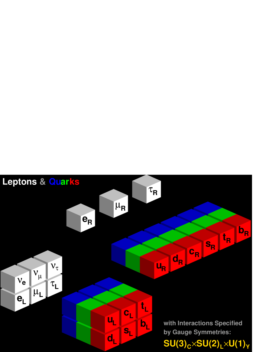
Figure 2.1: SU(3)_C$\times$SU(2)_L$\times$U(1)_Y gauge symmetries of fermions in the Standard Model. Quarks have three color degrees-of-freedom, while leptons are colorless. Left-handed fermions are arranged in SU(2) weak isospin doublets and right-handed fermions are arranged in SU(2) singlets. Each fermion also has U(1) weak hyper-charge. The interactions are uniquely specified by the gauge symmetries.

	$Q$	$T_{L}^{3}$	$Y$	$C$
$\nu_{e}$	0	1/2	-1	0
$e_{L}$	-1	-1/2	-1	0
$e_{R}$	-1	0	-2	0
$u_{L}$	2/3	1/2	1/3	$r,g,b$
$d_{L}$	-1/3	-1/2	1/3	$r,g,b$
$u_{R}$	2/3	0	4/3	$r,g,b$
$d_{R}$	-1/3	0	-2/3	$r,g,b$

Table 2.3: Quantum numbers of the fermions.

The interactions are uniquely specified by the SU(3)_C$\times$SU(2)_L$\times$U(1)_Y gauge symmetries. All of the gauge bosons and fermions acquire mass by the Higgs mechanism [4]. It introduces an extra Higgs boson, and its physical vacuum is spontaneously broken in the field space of the Higgs potential. The quark states in charged weak interactions mediated by $W^{\pm}$ bosons are not the physical states, but rather a quantum superposition of the physical states, described by the CKM (Cabbibo-Kobayashi-Maskawa) matrix [5].

$$\left(\begin{array}[]{c}d\\ s\\ b\end{array}\right)_{\mbox{weak}}=\left(\begin{array}[]{ccc}V_{ud}&V_{us}&V_{ub}\\ V_{cd}&V_{cs}&V_{cb}\\ V_{td}&V_{ts}&V_{tb}\end{array}\right)\left(\begin{array}[]{c}d\\ s\\ b\end{array}\right)_{\mbox{mass}}$$ (2.3)

The topic of this thesis is mostly related to the fermion couplings. The couplings to fermions in the SM are listed in Table 2.4. A very detailed review with explicit derivations on these topics starting from the gauge symmetry to the couplings to the fermions in the SM is given in Appendix B.

		Left Coupling	Right Coupling
Higgs	$H\to f\bar{f}$	$\frac{m_{f}}{v}$	$\frac{m_{f}}{v}$
Strong	$g\to q\bar{q}$	$\frac{g_{3}}{2}\lambda^{a}$	$\frac{g_{3}}{2}\lambda^{a}$
EM	$\gamma\to f\bar{f}$	$eQ_{f}$	$eQ_{f}$
Weak	$Z^{0}\to f\bar{f}$	$\frac{g_{2}}{\cos\theta_{W}}(T^{3}_{f}-\sin^{2}\theta_{W}Q_{f})$	$-\frac{g_{2}}{\cos\theta_{W}}\sin^{2}\theta_{W}Q_{f}$
	$W^{\pm}\to l\nu_{l}$	$\frac{g_{2}}{\sqrt{2}}$	0
	$W^{\pm}\to qq^{\prime}$	$V_{qq^{\prime}}\frac{g_{2}}{\sqrt{2}}$	0

Table 2.4: Couplings to fermions in the Standard Model.

In spite of its tremendous success in explaining collider results, there are still many unexplained aspects in the SM. The set of group representations and hypercharge it requires are quite bizarre, and there are 18 free parameters which must be input from experiment: 3 gauge couplings (usually traded as $e$, $\sin^{2}\theta_{W}$ and $g_{3}$), 2 Higgs potential couplings (usually traded as $m_{Z}$ and $m_{H}$), 9 fermion masses, and 4 CKM mixing parameters. Do particle masses really originate from a Higgs field? Can all the particle interactions be unified in a simple gauge group? What is the origin of the CKM matrix? The ultimate “theory of everything” should explain all of these parameters. The imaginary goal, for example, is probably to express everything in terms of the Planck constant $\hbar$, the speed of light $c$, the mathematical constant $\pi$, and without any free parameters. That would be an amazing accomplishment. There are still many things to do in particle physics in the direction to find the simplest model and many exciting challenges are ahead!

2.2 Extensions to the Standard Model

One interesting extension to the SM is to add a new U(1) gauge group. This predicts a new $Z^{\prime}$ gauge boson [6] at high energy scale. We will use the $Z^{\prime}$ as our model to calculate the signal acceptance for any kind of new vector boson.

Another interesting extension is supersymmetry [7], which is motivated by the desire to unify fermions and bosons, shown in Fig. 2.2.

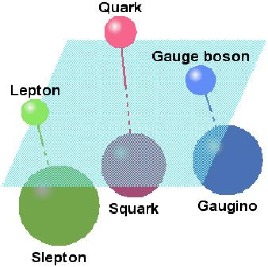
Figure 2.2: Particles in the Supersymmetry Theory.

For each fermion (lepton and quark) it predicts a bosonic super partner (slepton and squark), and for each gauge boson it predicts a fermionic super partner (gaugino). There is a divergence from scalar contributions to radiative corrections for the Higgs mass in the SM, while the new fermion loops appearing in supersymmetry have a negative sign relative to the scalar contributions, thus cancel the divergence. We will use the pseudoscalar Higgs particle $A$, one of the Higgs particles predicted in the minimal supersymmetric extension of the Standard Model (MSSM) [8] as our model to calculate the signal acceptance for any kind of new scalar boson.

2.3 High Mass Tau Pairs

At the Tevatron, the tau pair production in the SM is through the Drell-Yan process, $p\bar{p}\to\gamma^{*}/Z\to\tau\tau$, as shown in Fig. 2.4. The center-of-mass energy of $p\bar{p}$ collisions at the Tevatron is 1.96 TeV. At the parton level, one incoming quark from a proton and the other anti-quark from an anti-proton collide via an intermediate boson which decays to two outgoing taus. The details about how to calculate cross sections are shown in Appendix C and the mass spectrum of the final two taus is shown in Fig. 2.4. We perform a direct search for new hypothetical particle in high mass region by its decay to two taus $X\to\tau\tau$. The low mass region of the SM processes $\gamma^{*}/Z\to\tau\tau$ is the control region and its high mass Drell-Yan tail is the major background for this search.

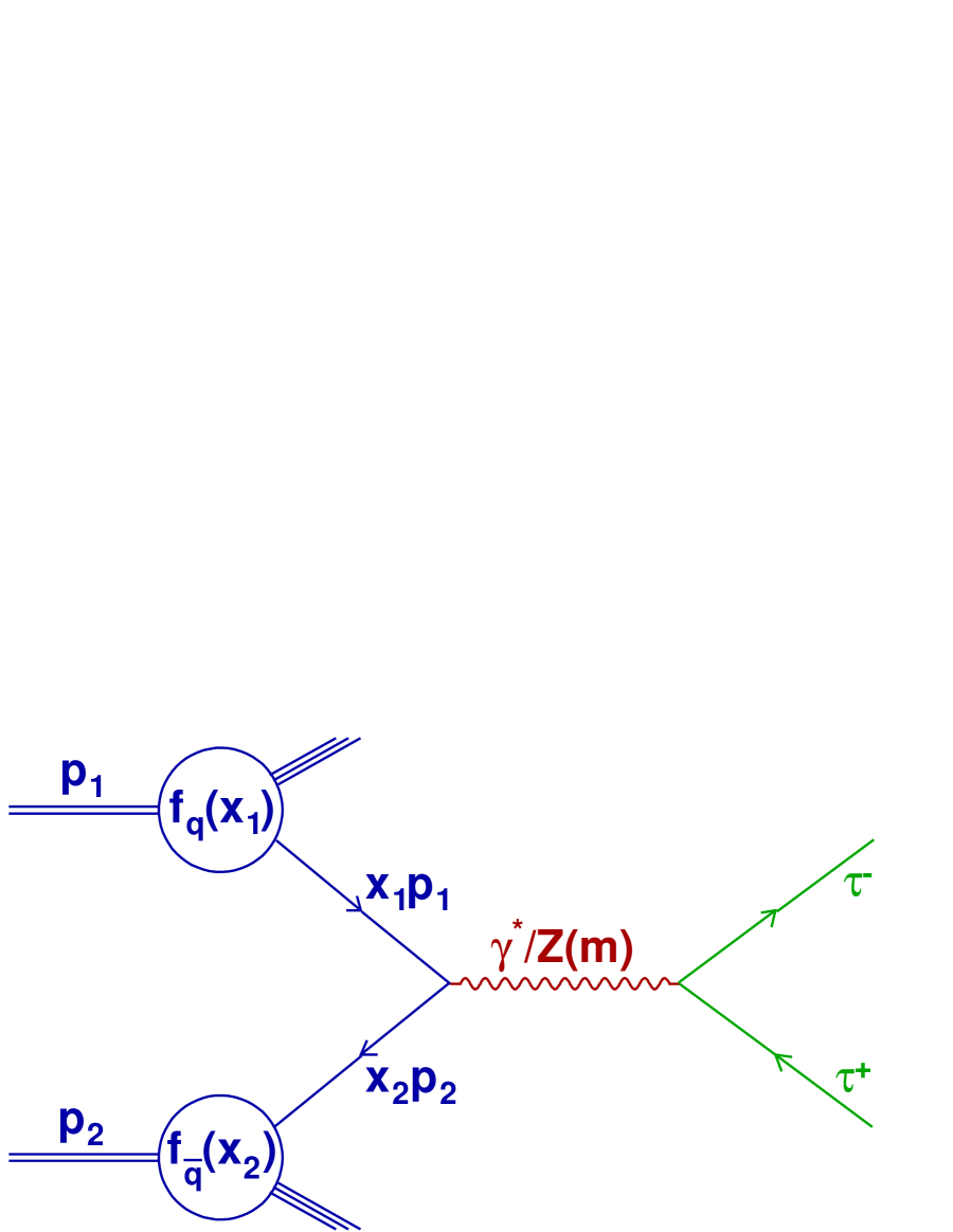
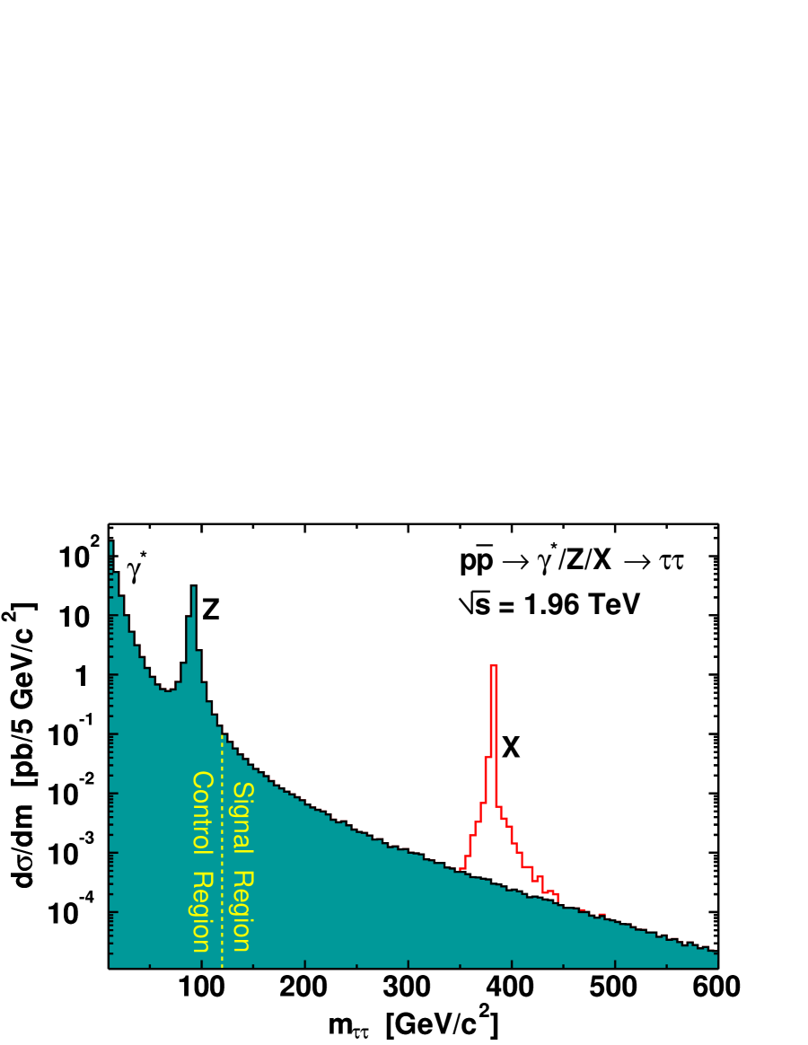
Figure 2.3: Tau pair production $p\bar{p}\to\gamma^{*}/Z\to\tau\tau$ in the Standard Model.

Figure 2.4: High mass tau pair search. Low-mass region including the $Z$ peak is the control region. High-mass region is the signal region. The high-mass tail of the Drell-Yan process is the main background of this search. The signature of new particles is a sigficant deviation from the known backgrounds, such as $X$ shown in this plot.

The two extensions described above are shown in Fig. 2.6. For U(1) extension, we consider the simplest model with the same interactions as the $Z$ boson in the SM, called the sequential $Z^{\prime}$, and the only unknown parameter is the mass of the new gauge boson. The MSSM requires two Higgs doublets and the ratio of the two Higgs expectation values is defined as $\tan\beta$, which is undetermined and should be treated as a free parameter. Thus the $A$ boson is governed by one more free parameter in addition to its mass.

The couplings to fermions in the SM are listed in Table 2.4. For each mass point of the sequential $Z^{\prime}$, we can use the same couplings to fermions as the $Z$ boson in the SM and repeat the procedure to calculate the cross section. The leading order cross section $\sigma_{0}$ is subject to a correction $K$ factor [9] such that the corrected cross section $\sigma=(1+\mbox{correction})\times\sigma_{0}=K\times\sigma_{0}$. Including the $K$ factor, the predicted cross section versus mass for the sequential $Z^{\prime}$ is shown in Fig. 2.6.

The SM requires one Higgs doublet with a coupling of the SM Higgs boson to fermions as $m_{f}/v$, where $m_{f}$ is the fermion mass and $v$ is the vacuum expectation value of the SM Higgs boson, about 246 GeV. Therefore Higgs boson prefers to couple to the fermions in the heaviest generation. In the MSSM, at large $\tan\beta$, the coupling of $A\to\tau\tau$ and $A\to b\bar{b}$ are enhanced to $m_{f}\tan\beta/v$, whereas the coupling of $A\to t\bar{t}$ is suppressed to $m_{t}\cot\beta/v$ when the top quark is kinematically available, i.e. $m_{A}>2m_{t}\approx 350$ GeV/$c^{2}$. We use the programs HIGLU [10] and HDECAY [11] to calculate the next-to-leading-order cross section of $gg\to A\to\tau\tau$. They are also shown in Fig. 2.6.

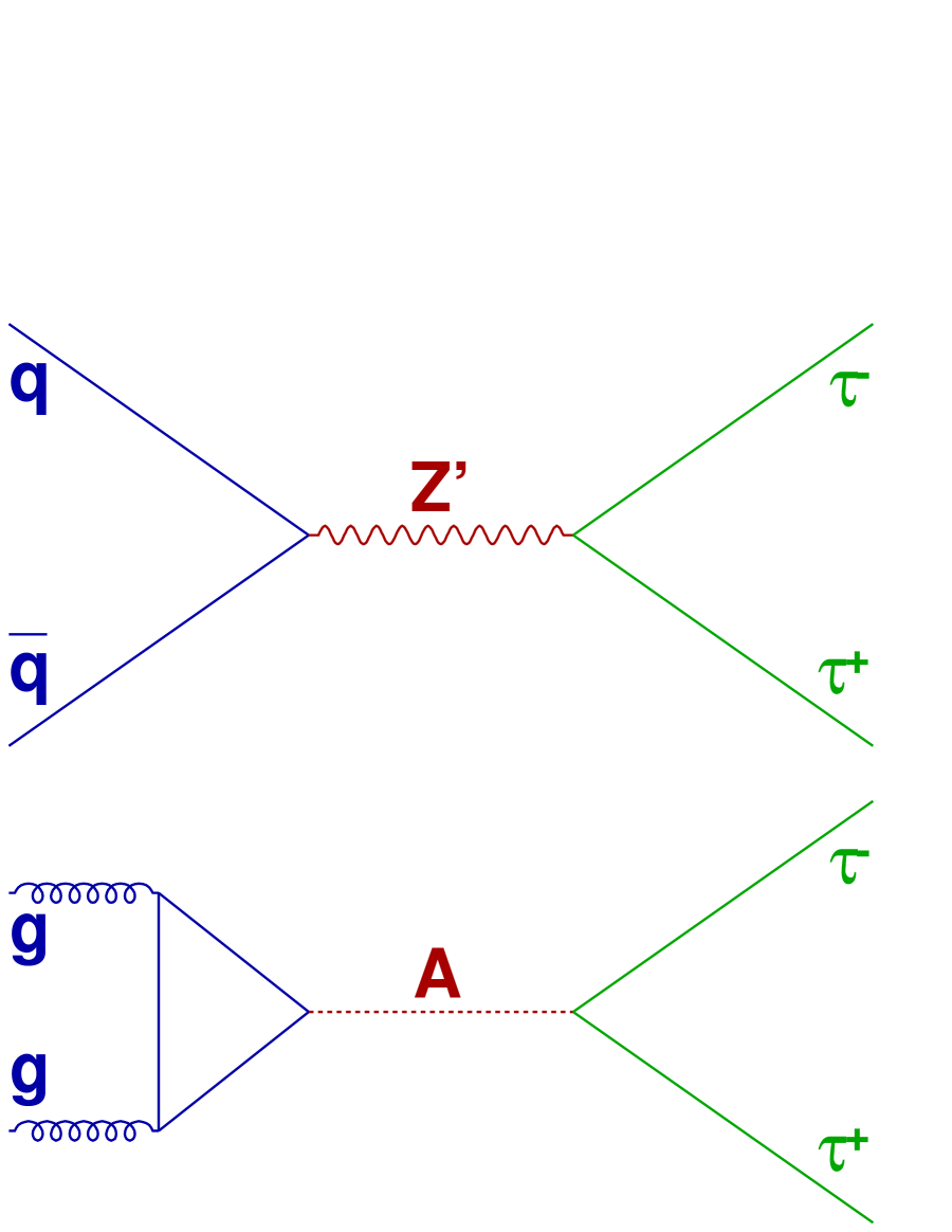
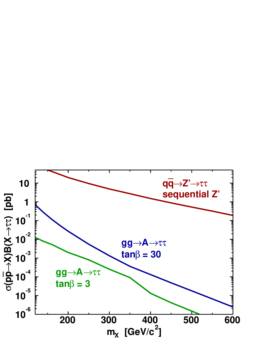
Figure 2.5: Tree-level Feynman diagrams for the productions at $p\bar{p}$ collider and decays of $Z^{\prime}$ predicted in U(1) extension and pseudoscalar $A$ predicted in minimum supersymmetric extension of the Standard Model.

Figure 2.6: Theoretical signal $\sigma(p\bar{p}\to X)\cdot\mbox{B}(X\to\tau\tau)$.

Chapter 3 The Tevatron Accelerator and the CDF Detector

Fermilab is the home of the highest energy particle accelerator in the world, the Tevatron. The center-of-mass energy of proton-antiproton ($p\bar{p}$) collision is $\sqrt{s}=1.96$ TeV. We shall describe the Tevatron accelerator and the Collider Detector at Fermilab (CDF) in this chapter.

3.1 Fermilab’s Accelerator Chain

Protons and antiprotons have equal and opposite electric charge. The advantage of $p\bar{p}$ collider is that $p$ and $\bar{p}$ travel in opposite directions through the magnets and a $p\bar{p}$ collider can be built with one ring of magnets instead of two. The disadvantage is that it is difficult to produce and accumulate $\bar{p}$ at a high efficiency.

The aerial view of Fermilab is shown in Fig. 3.2. The Fermilab’s accelerator chain is shown in Fig. 3.2. It consists of the Proton/Antiproton Sources (8 GeV), the Main Injector (150 GeV), the Recycler, and the Tevatron (980 GeV).

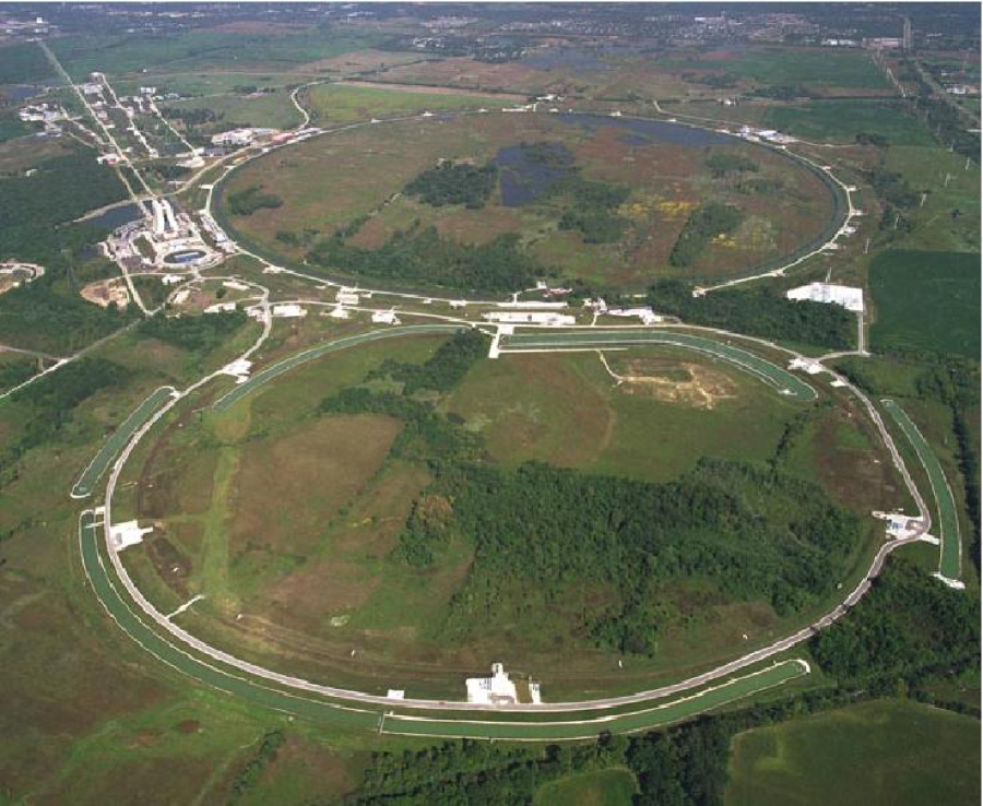
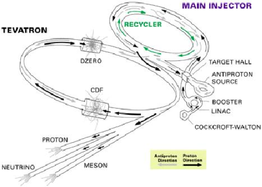
Figure 3.1: Aerial view of Fermilab showing the Main Injector in the foreground, the Tevatron collider ring and the fixed target facilities in the background.

Figure 3.2: Fermilab’s accelerator chain consists of the 8 GeV proton source, the 8 GeV anti-proton source, the Main Injector, the Recycler for recycling the precious anti-protons, and the Tevatron. The Main Injector accelerates protons and anti-protons to 150 GeV. The Tevatron ramps up their energies to 980 GeV. The center-of-mass energy of $p\bar{p}$ collision is thus 1.96 TeV. The linear accelerators for the fixed targed experiments are also shown.

The Proton Source includes the Cockcroft-Walton, the Linear Accelerator (Linac), and the Booster. The Cockcroft-Walton uses DC power to accelerate H^- ions to 750 KeV. The Linac uses Radio Frequency (RF) power to accelerate H^- ions to 400 MeV. The electrons are stripped off and the bare protons are injected into the Booster. The Booster uses RF cavities to accelerate protons to 8 GeV.

The Anti-proton Source includes the Target Station, the Debuncher and the Accumulator. A bunched beam of 120 GeV protons from the Main Injector hits a Nickel Target to make anti-protons and other particles as well. The particles are focused with a lithium lens and filtered through a pulsed magnet acting as a charge-mass spectrometer to select anti-protons. The antiproton beam is bunched since the beam from the Main Injector is bunched and the antiprotons have a wide range of energies, positions and angles. The transverse spread of the beam out of the Target Station is “hot”, in terms analogous to temperature. Both RF and stochastic cooling systems are used in the momentum stacking process. The Debuncher exchanges the large energy spread and narrow time spread into a narrow energy spread and large time spread. The Accumulator stacks successive pulses of antiprotons from the Debuncher over several hours or days. For every million protons that hit the target, only about twenty 8 GeV anti-protons finally get stacked into the Accumulator.

Protons at 8 GeV from the Booster are injected into the Main Injector. They are accelerated to 120 GeV for fixed target experiments or 150 GeV for injection into the Tevatron. Antiprotons at 8 GeV from either the Accumulator or the Recycler are accelerated to 150 GeV in the Main Injector and then injected into the Tevatron.

The Recycler is placed directly above the Main Injector beamline, near the ceiling. One role of the Recycler is a post-Accumulator ring. Another role, and by far the leading factor in the luminosity increase, is to act as a recycler for the precious antiprotons left over at the end of Tevatron stores. It is a ring of steel cases holding bricks of “refrigerator” magnets (the same permanent magnet used in home refrigerators). Permanent magnets do not need power supplies, cooling water systems, or electrical safety systems. The Recycler is a highly reliable storage ring for antiprotons.

The Tevatron was the world’s first superconducting synchrotron. A magnet with superconducting coils has no electrical resistance, and consumes minimal electrical power, except that is needed to keep the magnets cold. The particles of a beam are guided around the closed path by dipole magnetic field. The radius of the circle is 1000 meters. As the beam energy is ramped up by RF cavities from 150 GeV to 980 GeV, the bending magnetic field and the RF frequency must be synchronized to keep the particles in the ring and this enables a stable longitudinal motion. The stability of the transverse motion is achieved with a series quadrupole magnets with alternating gradient.

Luminosity is a measure of the chance that a proton will collide with an antiproton. To achieve high luminosity we place as many particles as possible into as small a collision region as possible. At the interaction point, the two beams of $p$ and $\bar{p}$ are brought together by special quadrupole magnets called Low Beta magnets, shown in Fig. 3.3.

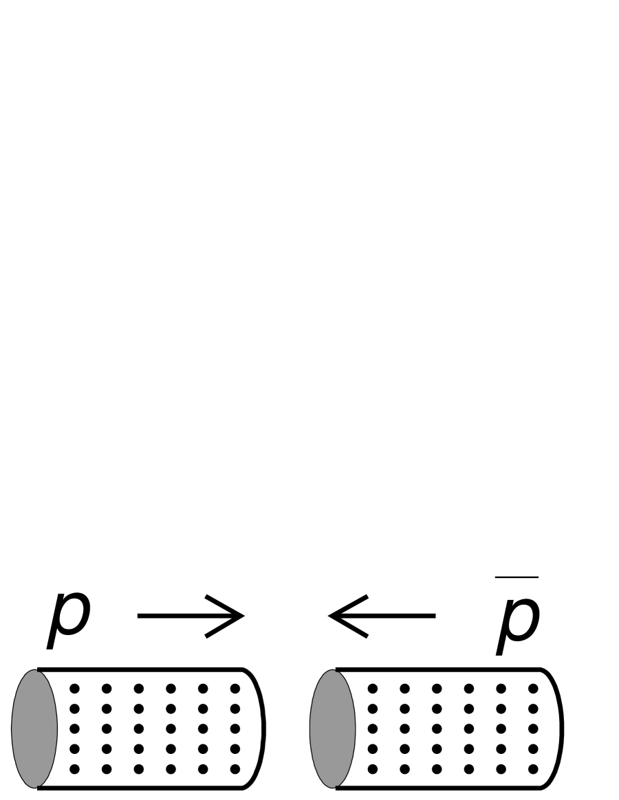
Figure 3.3: $p\bar{p}$ collision.

The current status (at the writing of the thesis) of the luminosity is shown in Fig. 3.5, and the integrated luminosity delivered and to tape is shown in Fig. 3.5.

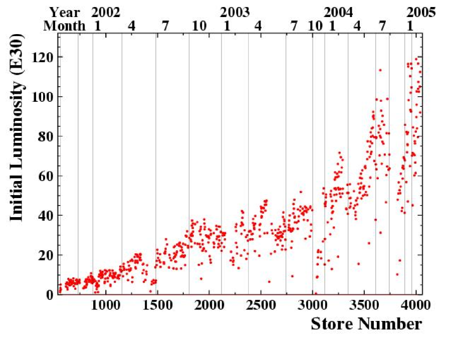
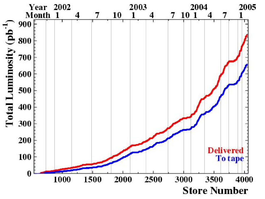
Figure 3.4: Run II instantaneous initial luminosity.

Figure 3.5: Run II integrated luminosity.

The design value for the peak instantaneous luminosity during Run II is $2\times 10^{32}$ cm^-2s^-1. Typically a year allows 10⁷ seconds of running at the peak instantaneous luminosity. This is about one third of the actual number of seconds in a year, which accounts both for the drop in luminosity and for a normal amount of down-time. Using the conversion constant $1\mbox{ fb}=10^{-39}\mbox{ cm}^{2}$, the design value corresponds to an integrated luminosity about 2 fb^-1 per year. Ultimately it is hoped that an integrated luminosity of 8$-$10 fb^-1 can be attained in Run II. The total number of events $N$ in a scattering process is proportional to the luminosity and the cross section $\sigma$ of the process,

$$N=L\sigma$$ (3.1)

We can get a rough sense of the reach for new physics and the challenge of enhancing signal and suppressing background by considering the following examples. At a center-of-mass energy of 1.96 TeV, we have

$$\sigma(p\bar{p}\to\mbox{anything}) \approx 75\mbox{ mb}$$ (3.2)

$$\sigma(p\bar{p}\to t\bar{t}+\mbox{anything}) \approx 6\mbox{ pb}$$ (3.3)

$$\sigma(p\bar{p}\to hZ+\mbox{anything}) \approx 75\mbox{ fb}$$ (3.4)

3.2 The CDF Dectector

The CDF detector [12] is cylindrically symmetric around the beamline. A solid cutaway view is shown in Fig. 3.7, and an elevation view is shown in Fig. 3.7. It is a general-purpose solenoidal detector with tracking system, calorimetry and muon detecion. The tracking system is contained in a superconducting solenoid, 1.5 m in radius and 4.8 m in length. The magnetic field is 1.4 T, parallel to the beamline. The calorimetry and muon system are outside the solenoid. These sub-systems will be described in more details below.

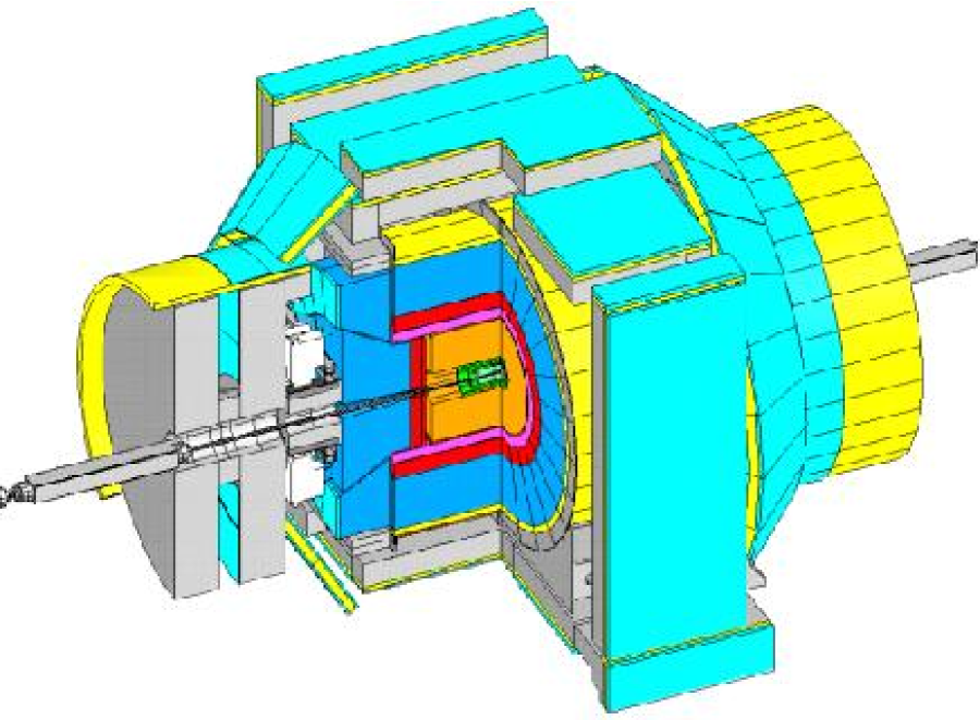
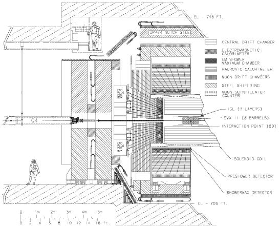
Figure 3.6: Solid cutaway view of CDF II detector.

Figure 3.7: Elevation view of CDF II detector.

3.2.1 CDF Coordinate System

The origin of the CDF detector is its geometric center. The luminous region of the beam at the interaction point has Gaussian profiles with $(\sigma_{x},\;\sigma_{y},\;\sigma_{z})_{beam}\approx(0.003,\;0.003,\;30)$ cm. The $p\bar{p}$ collision point is not necessarily at the origin.

The CDF detector uses a right-handed coordinate system. The horizontal direction pointing out of the ring of the Tevatron is the positive $x$-axis. The vertical direction pointing upwards is the positive $y$-axis. The proton beam direction pointing to the east is the positive $z$-axis.

A spherical coordinate system is also used. The radius $r$ is measured from the center of the beamline. The polar angle $\theta$ is taken from the positive $z$-axis. The azimuthal angle $\phi$ is taken anti-clockwise from the positive $x$-axis.

At a $p\bar{p}$ collider, the production of any process starts from a parton-parton interaction which has an unknown boost along the $z$-axis, but no significant momentum in the plane perpendicular to the $z$-axis, i.e. the transverse plane. This makes the transverse plane an important plane in $p\bar{p}$ collision. Momentum conservation requires the vector sum of the transverse energy and momentum of all of the final particles to be zero. The transverse energy $E_{T}$ and transverse momentum $p_{T}$ are defined by

$$E_{T} = E\sin\theta$$ (3.5)

$$p_{T} = p\sin\theta$$ (3.6)

Hard $p\bar{p}$ head-on collisions produce significant momentum in the transverse plane. The CDF detector has been optimized to measure these events. On the other hand, the soft collisions such as elastic or diffractive interactions or minimum-bias events, and by-products from the spectator quarks from hard collisions, have most of their energy directed along the beampipe, and will not be measured by the detector.

Pseudorapidity $\eta$ is used by high energy physicists and is defined as

$$\eta=-\ln\tan\frac{\theta}{2}$$ (3.7)

Consider occupancy in a sample of large amount of $p\bar{p}$ collision events. Typically, particles in a $p\bar{p}$ collision event tend to be more in the forward and backward regions than in the central region because there is usually a boost along the $z$-axis, which could be shown in $\theta$ occupancy of the particles of the events in the sample. Now we transform $\theta$ to $\eta$. The derivative of $\eta$ is

$$d\eta=-\frac{d\theta}{\sin\theta}$$ (3.8)

A constant $\eta$ slice corresponds to variant $\theta$ slice which is smaller in the forward and backward regions than in the central region. This can make the $\eta$ occupancy more uniform than $\theta$ occupancy. For example, calorimeters are constructed in $\eta$ slices, instead of $\theta$ slices.

3.2.2 Tracking

The tracking volume is surrounded by the solenoid magnet and the endplug calorimeters as shown in Fig. 3.8. The tracking system records the paths of charged particles produced in the $p\bar{p}$ collisions. It consists of a silicon microstrip system [13] with radius from $r=1.5$ to 28 cm and $|\eta|<2$, and an open-cell wire drift chamber called central outer tracker (COT) [14] with radius from $r=40$ to 137 cm and $|\eta|<1$.

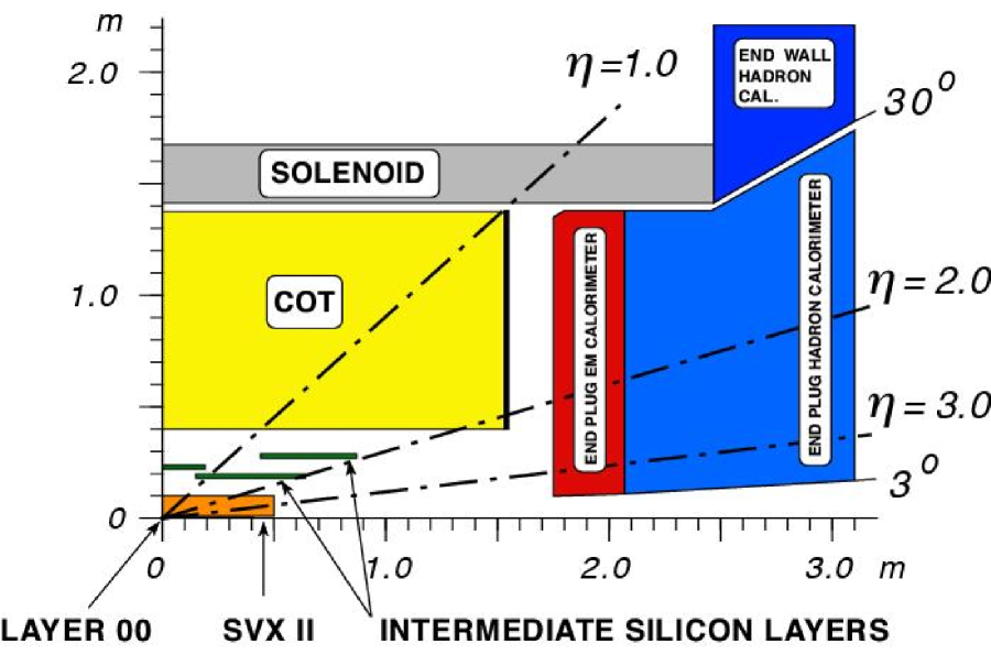
Figure 3.8: CDF II tracking volume.

The silicon microstrip is made from Si with a p-n junction. When p-type semiconductors and n-type semiconductors are brought together to form a p-n junction, migration of holes and electrons leaves a region of net charge of opposite sign on each side, called the depletion region (depleted of free charge carriers). The p-n junction can be made at the surface of a silicon wafer with the bulk being n-type (or the opposite way). By applying a reverse-bias voltage we can increase the depletion region to the full volume of the device. A charged particle moves through this depletion region, creates electron-hole pairs which drift and are collected at the surfaces. This induces a signal on metal strips deposited on the surface, connected to readout amplifiers.

The silicon microstrip detector consists of three components: the Layer 00, the Silicon VerteX detector II (SVX II), and the Intermediate Silicon Layers (ISL). An end view is shown in Fig. 3.10. Layer 00 is physically mounted on and supported by the beam pipe. The sensors are single-sided p-in-n silicon and have a pitch of 25 $\mu$m. The next five layers compose the SVX II and are double-sided detectors. The axial side of each layer is used for $r$-$\phi$ measurements and the sensors have a strip pitch of about 60 $\mu$m. The stereo side of each layer is used for $r$-$z$ measurements. Both 90^∘ and small-angle stereo sensors are used in the pattern (90, 90, $-$1.2, 90, +1.2) degrees and have a strip pitch of (141, 125.5, 60, 141, 60) $\mu$m from the innermost to outermost layers. The two outer layers compose the ISL and are double-sided detectors with a strip pitch of 112 $\mu$m on both the axial and the 1.2^∘ stereo sides. This entire system allows charged particle track reconstruction in three dimensions. The impact parameter resolution of SVX II + ISL is 40 $\mu$m including 30 $\mu$m contribution from the beamline. The $z_{0}$ resolution of SVX II + ISL is 70 $\mu$m.

The COT is arranged in 8 superlayers shown in Fig. 3.10. The superlayers are alternately axial and $\pm$2^∘ stereo, four axial layers for $r$-$\phi$ measurement and four stereo layers for $r$-$z$ measurement. Within each superlayer are cells which are tilted about 30^∘ to the radial direction to compensate for the Lorentz angle of the drifting charged particles due to the solenoid magnet field. Each cell consists of 12 layers of sense wires, thus total 8$\times$12 = 96 measurements per track.

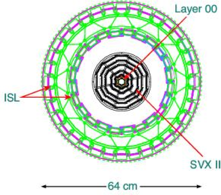
Figure 3.9: Silicon system.

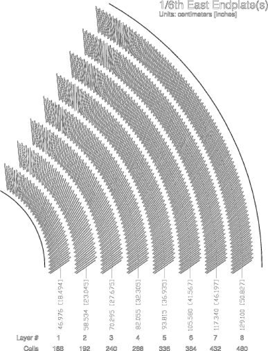
Figure 3.10: COT superlayers.

The COT is filled with a mixture of argone:ethane = 50:50 which determines the drift velocity $v$. A charged particle enters gas, ionizes gas and produces electrons. There is an electric field around each sense wire. In the low electric field region, the ionization electrons drift toward the sense wire. In the high electric field region within a few radii of the sense wire, there is an avalanche multiplication of charges by electron-atom collision. A signal is induced via the motion of electrons. By measuring the drift time $t$ (the arrival time of “first” electrons) at sense wire relative to collision time $t_{0}$, we can calculate the distance of the hit $D=v\Delta t$.

A track is formed from a series of hits, fit to a helix. We can measure the curvature of a track $C=1/R$ and then calculate transverse momentum $p_{T}=0.3$$R$$B$, with $p_{T}$, $R$ and $B$ in the units GeV/$c$, m, and T, respectively. The hit position resolution is approximately 140 $\mu$m and the momentum resolution $\sigma(p_{T})/p_{T}^{2}$ = 0.0015 (GeV/$c$)^-1.

3.2.3 Calorimetry

The CDF electromagnetic and hadronic sampling calorimeters surround the tracking system and measure the energy flow of interacting particles up to $|\eta|<3.64$. They are segmented in $\eta$ and $\phi$ with a projective “tower” geometry, shown in Fig. 3.11.

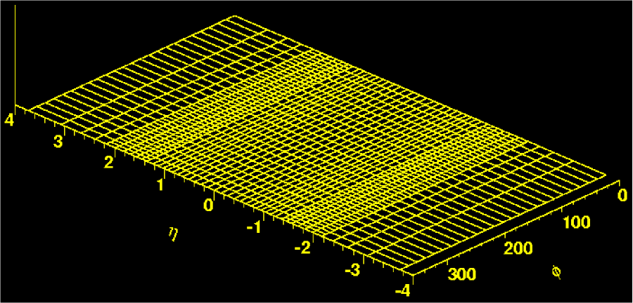
Figure 3.11: Calorimeter tower segmentation in $\eta-\phi$ space.

The energy measurement is done by sampling calorimeters which are absorber and sampling scintillator sandwich with phototude readout. When interacting with the absorber, electrons lose energy by ionization and bremsstrahlung, and photons lose energy by the photoelectric effect, Compton scattering and pair production. Both electrons and photons develop electromagnetic shower cascades. The size of the longitudinal shower cascade grows only logarithmically with energy. A very useful cascade parameter is the radiation length $X_{0}$ which is the mean distance for the $e^{\pm}$ to lose all but 1/e of its energy. For example, for a 10 GeV electron in lead glass, the maximum electromagnetic shower is at about 6$X_{0}$ and the 95% containment depth is at about 16$X_{0}$. Hadrons lose energy by nuclear interaction cascades which can have charged pions, protons, kaons, neutrons, neutral pions, neutrinos, soft photons, muons, etc. It is much more complicated than an electromagnetic cascade and thus results in a large fluctuation in energy measurement. In analogy to $X_{0}$, a hadronic interaction length $\lambda$ can be defined. Hadronic showers are much longer than the electromagnetic ones.

The central calorimeters consist of the central electromagnetic calorimeter (CEM) [15], the central hadronic calorimeter (CHA) [16], and the end wall hadronic calorimeter (WHA). At approximately 6$X_{0}$ in depth in the CEM, at which electromagnetic showers typically reach the maximum in their shower profile, is the central shower maximum detector (CES). The CEM and CHA are constructed in wedges which span 15^∘ in azimuth and extend about 250 cm in the positive and negative $z$ direction, shown in Fig. 3.15. There are thus 24 wedges on both the $+z$ and $-z$ sides of the detector, for a total of 48. A wedge contains ten towers, each of which covers a range 0.11 in pseudorapidity. Thus each tower subtends $0.11\times 15^{\circ}$ in $\eta\times\phi$. CEM covers $0<|\eta|<1.1$, CHA covers $0<|\eta|<0.9$, and WHA covers $0.7<|\eta|<1.3$.

The CEM uses lead sheets interspersed with polysterene scintillator as the active medium and employs phototube readout, approximately 19$X_{0}$ in depth, and has an energy resolution $13.5\%/\sqrt{E_{T}}\oplus 2\%$, where $\oplus$ denotes addition in quadrature. The CES uses proportional strip and wire counters in a fine-grained array, as shown in Fig. 3.15, to provide precise position (about 2 mm resolution) and shape information for electromagnetic cascades. The CHA and WHA use steel absorber interspersed with acrylic scintillator as the active medium. They are approximately 4.5$\lambda$ in depth, and have an energy resolution of $75\%/\sqrt{E_{T}}\oplus 3\%$.

The plug calorimeters consist of the plug electromagnetic calorimeter (PEM) [17], and the plug hadronic calorimeter (PHA). At approximately 6$X_{0}$ in depth in PEM is the plug shower maximum detector (PES). Fig. 3.15 shows the layout of the detector and coverage in polar angle $36.8^{\circ}>\theta>3^{\circ}$ ($1.1<|\eta|<3.64$). Each plug wedge spans 15^∘ in azimuth, however in the range $36.8^{\circ}>\theta>13.8^{\circ}$ ($1.1<|\eta|<2.11$) the segmentation in azimuth is doubled and each tower spans only 7.5^∘.

The PEM is a lead-scintillator sampling calorimeter. It is approximately 21$X_{0}$ in depth, and has an energy resolution of $16\%/\sqrt{E}\oplus 1\%$. The PES consists of two layers of scintillating strips: U and V layers offset from the radial direction by $+22.5^{\circ}$ and $-22.5^{\circ}$ respectively, as shown in Fig. 3.15. The position resolution of the PES is about 1 mm. The PHA is a steel-scintillator sampling calorimeter. It is approximately 7$\lambda$ in depth, and has an energy resolution of $74\%/\sqrt{E}\oplus 4\%$.

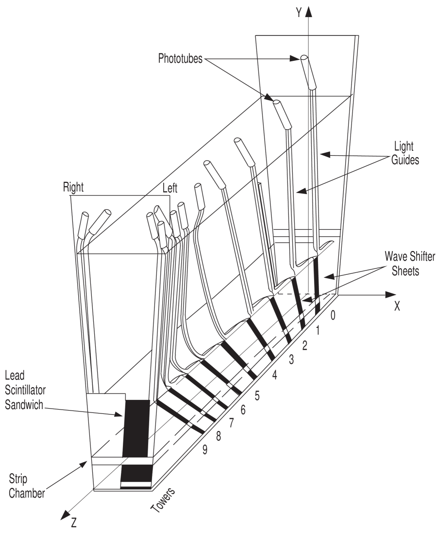
Figure 3.12: CEM/CES/CHA wedge.

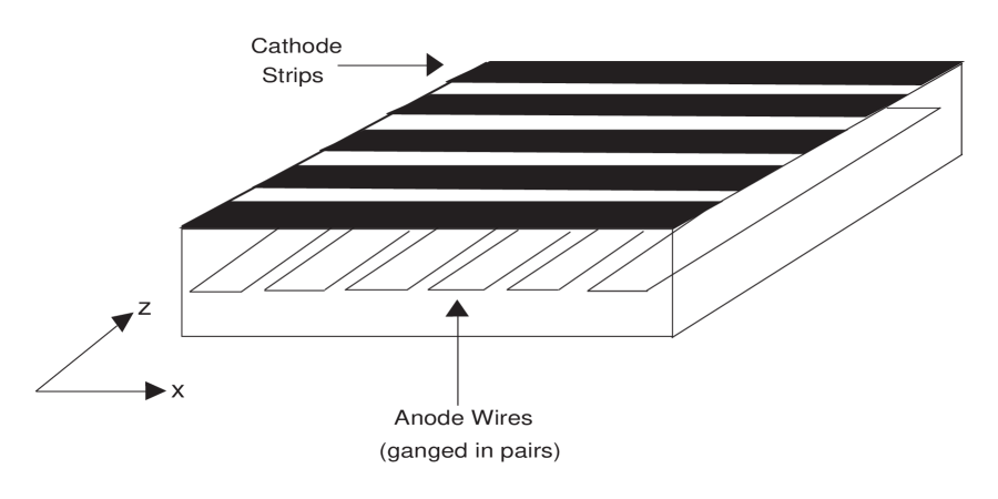
Figure 3.13: CES strip and wire.

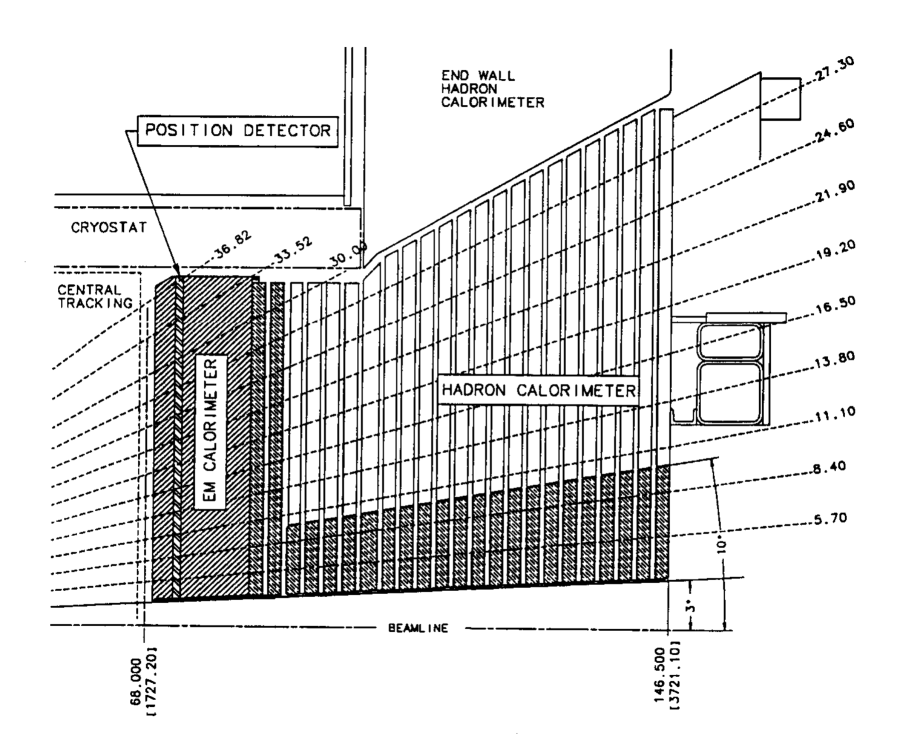
Figure 3.14: PEM/PES/PHA layout.

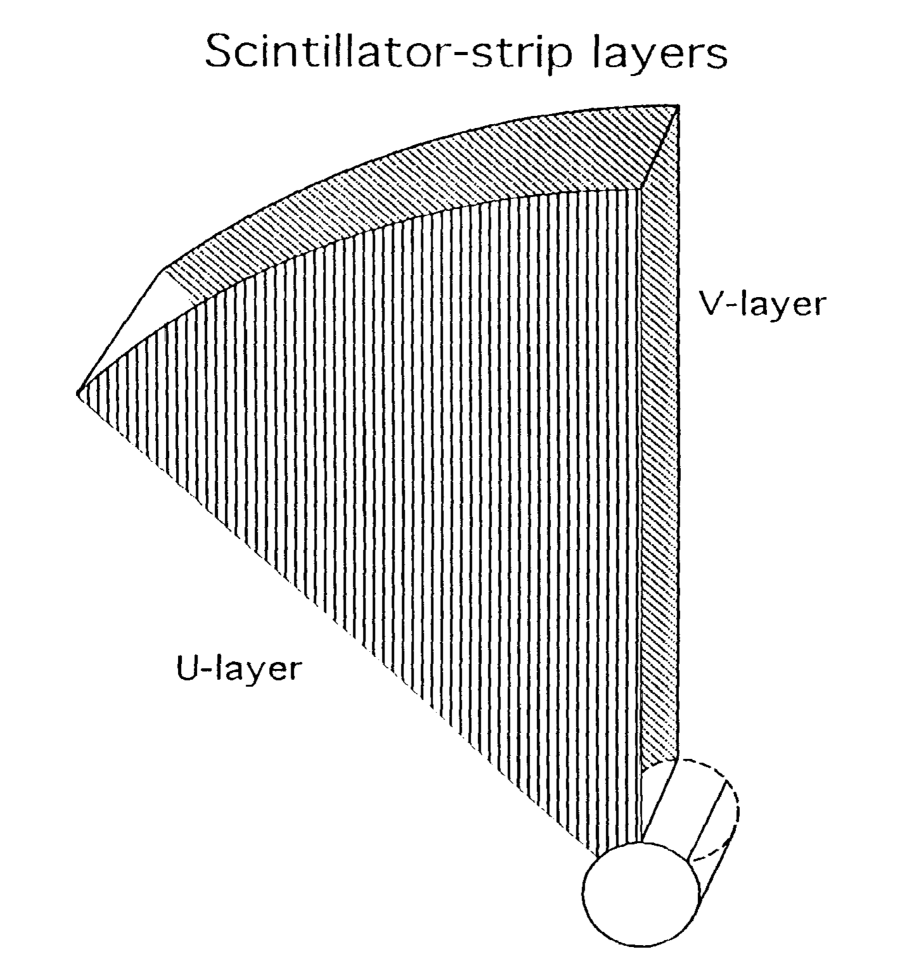
Figure 3.15: PES U and V layers.

3.2.4 Muon Chambers

The muon chambers are situated outside the calorimeters. In addition to the calorimeters, the magnet return yoke and additional steel shielding are used to stop electrons, photons and hadrons from entering the muon chambers. The muon is a minimum ionizing particle which loses very little energy in detector materials. The muon’s lifetime is long enough to allow it to pass through all the detector components, reach the muon chambers, and decay outside.

A muon chamber contains a stacked array of drift tubes and operates with a gas mixture of argon:ethane = 50:50. The basic drift principle is the same as that of the COT, but the COT is a multi-wire chamber, while at the center of a muon drift tube there is only a single sense wire. The sense wire is connected to a positive high voltage while the wall of the tube is connected to a negative high voltage to produce a roughly uniform time-to-distance relationship throughout the tube. The drift time of a single hit gives the distance to the sense wire, and the charge division at each end of a sense wire can in principle be used to measure the longitudinal coordinate along the sense wire. The hits in the muon chamber are linked together to form a short track segment called a muon stub. If a muon stub is matched to an extrapolated track, a muon is reconstructed. This is shown in Fig. 3.16.

Figure 3.16: Muon stub matching to a track.

There are four independent muon detectors: the central muon detector (CMU) [18], the central muon upgrade (CMP), the central muon extension (CMX), and the intermediate muon detector (IMU). The muon coverage in $\eta-\phi$ space is shown in Fig. 3.17.

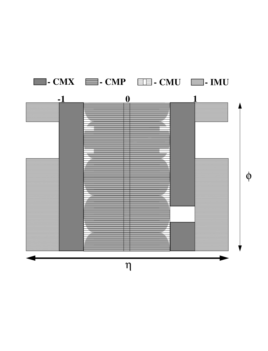
Figure 3.17: Muon coverage in $\eta$ and $\phi$.

The CMU is behind the central hadronic calorimeter and has four layers of cylindrical drift chambers. The CMP is behind an additional 60 cm of shielding steel outside the magnet return yoke. It consists of a second set of four layers with a fixed length in $z$ and forms a box around the central detector. Its psuedorapidity coverage thus varies with the azimuth. A layer of scintillation counters (the CSP) is installed on the outside surface of the CMP. The CMU and CMP each covers $|\eta|<0.6$. The maximum drift time of the CMU is longer than the $p\bar{p}$ bunch crossing separation. This can cause an ambiguity in the Level 1 trigger (described in the next section) about which bunch the muon belongs to. By requiring CMP confirmation, this ambiguity is resolved by the CSP scintillators.

The CMX has eight layers and covers $0.6<|\eta|<1.0$. A layer of scintillation counters (the CSX) is installed on both the inside and the outside surfaces of the CMX. No additional steel was added for this detector because the large angle through the hadron calorimeter, magnet yoke, and steel of the detector end support structure provides more absorber material than in the central muon detectors. The azimuthal coverage of CMX has a 30^∘ gap for the solenoid refrigerator.

The IMU consists of barrel chambers (the BMU) and scintillation counters (the BSU), and covers the region $1.0<|\eta|<1.5$.

3.3 Trigger and Data Acquisition System

The trigger system has a three-level architecture: level 1 (L1), level 2 (L2), and level 3 (L3). The data volume is reduced at each level which allows more refined filtering at subsequent levels with minimal deadtime. The trigger needs to be fast and accurate to record as many interesting events as possible, while rejecting uninteresting events.

Each sub-detector generates primitives that we can “cut” on. The trigger system block diagram is shown in Fig. 3.18. The available trigger primitives at L1 are

• XFT tracks, with $\phi$ and $p_{T}$ provided by the eXtreme Fast Tracker using the hits in the axial layers of the COT,

• electrons, based on XFT and HAD/EM which is the ratio of the hadronic energy and the electromagnetic energy of a calorimeter tower,

• photons, based on HAD/EM ratio,

• jets, based on EM+HAD,

• muons, based on muon hits and XFT, and

• missing $E_{T}$ and sum $E_{T}$ which are the negative of the vector sum and the scalar sum of the energies of all of the calorimeter towers, respectively.

The available trigger primitives at L2 are

• SVT, the Silicon Vertex Tracker trigger based on the track impact parameter of displaced tracks,

• jet clusters,

• isolated clusters, and

• EM ShowerMax which is the strip and wire clusters in the CES.

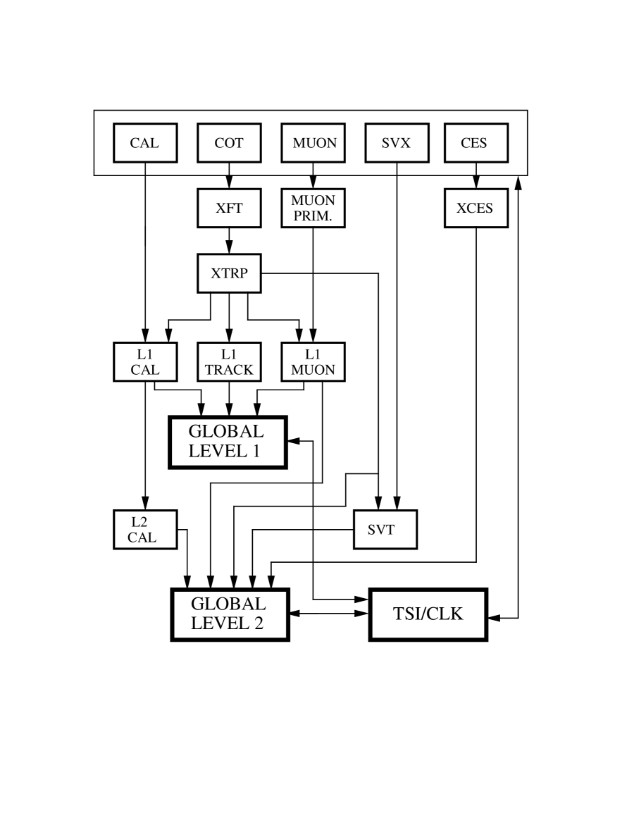
Figure 3.18: Trigger system block diagram.

There are two important factors for trigger design: the time between beam crossing and $\bar{N}$, the average number of overlapping interactions in a given beam crossing.

We can have many bunches in the Tevatron to enhance the luminosity. Since the radius of the ring is 1000 m, a proton (or an anti-proton) at a speed very close to the speed of light circulates the ring once every 20 $\mu$s. To accomodate 36 bunches, the maximum bunch separation allowed is about 600 ns, and the Run IIa configuration is 396 ns. The bunch separation defines an overall time constant for signal integration, data acquisition and triggering.

Another key design input is the average number of overlapping interactions $\bar{N}$, which is shown as a function of luminosity and the number of bunches in Fig. 3.19 [19]. For example, with 36 bunches, $\bar{N}$ is about 1 at $3\times 31$ cm^-2s^-1 and about 10 at $4\times 32$ cm^-2s^-1. The trigger with fast axial tracking at L1 can handle the former environment, but cannot handle the latter environment because of the presence of too many fake tracks. To be able to handle $4\times 32$ cm^-2s^-1 we would need 108 bunches and even that seems not enough, thus we will also need to upgrade the trigger to include, for example, stereo tracking at L1 to suppress fake tracks.

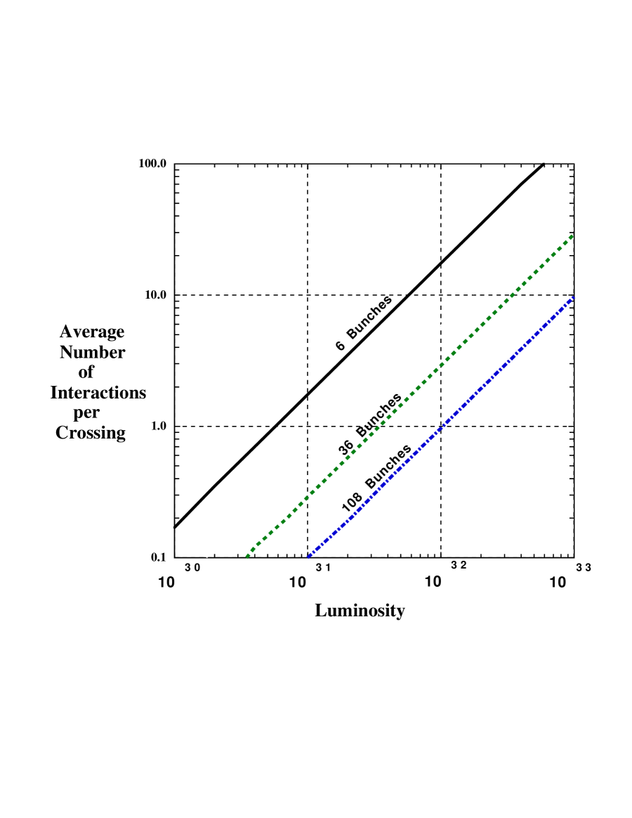
Figure 3.19: Average number of interactions per crossing for various bunches, as a function of instantaneous luminosity.

The data flow in the trigger system is constrained by the processing time, i.e. how fast a decision can be made to clear events at each level and the tape writing speed for permanant storage at the end of the triggering process. The implementation needs a sufficient buffer while filtering because any overflow means deadtime. The “deadtimeless” design for 132 ns crossing is shown in Fig. 3.20.

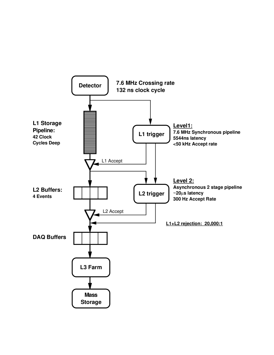
Figure 3.20: Data flow of “deadtimeless” trigger and data acquisition.

The L1 decision occurs at a fixed time about 5.5 $\mu$s after beam collision. L1 is a synchronous hardware trigger. To process one event every 132 ns, each detector element is pipelined to have local data buffering for 42 beam crossings. The L1 accept rate is less than 50 KHz which is limited by the L2 processing time.

The L2 decision time is about 20 $\mu$s. L2 is a combination of hardware and software triggers and is asynchronous. If an event is accepted by L1, the front-end electronics moves the data to one of the four onboard L2 buffers. This is sufficient to process a L1 50 KHz accept rate and to average out the rate fluctuations. The L2 accept rate is about 300 Hz which is limited by the speed of the event-builder in L3.

L3 is purely a software trigger consisting of the event builder running on a large PC farm. The event builder assembles event fragments from L1 and L2 into complete events, and then the PC farm runs a version of the full offline reconstruction code. This means that fully reconstructed three-dimensional tracks are available to the trigger decision. The L3 accept rate is about 75 Hz which is limited by tape writing speed for permanent storage.

Once an event passes L3 it is delivered to the data-logger sub-system which sends the event out to permanent storage for offline reprocess, and to online monitors which verify the entire detector and trigger systems are working properly.

The data used in this analysis were collected from March 2002 to September 2003. It was for 396 ns with 36 bunches and for luminosity about $3\times 31$ cm^-2s^-1. This means that the trigger (designed for 132 ns) was sufficiently capable to handle the timing of bunch crossing with no need to worry about multiple interactions in this environment.

Chapter 4 Search Strategy

This chapter describes the overall logic of the high-mass tau tau search. There are three steps:

1. Use $W\to\tau\nu$ events to cross check the $\tau$ identification efficiency.

2. Use $Z\to\tau\tau$ events to study the low-mass control region with $m_{vis}<$ 120 GeV/$c^{2}$.

3. Examine the high-mass signal region with $m_{vis}>$ 120 GeV/$c^{2}$ for evidence of an excess signalling new physics.

Tau Hadronic Decays

The dominant decays of $\tau$’s are into leptons or into either one or three charged hadrons, shown in Table 4.1. The following short-hand notations for $\tau$ and its decays are used,

$$\tau_{e} \tau\to e\bar{\nu}\nu$$ (4.1)

$$\tau_{\mu} \tau\to\mu\bar{\nu}\nu$$ (4.2)

$$\tau_{h} \tau\to\mbox{hadrons}~{}\nu$$ (4.3)

The leptonic decays cannot be distinguished from prompt leptons. So tau identification requires a hadronic tau decay only, with a mass less than

$$m(\tau)=1.777\mbox{ GeV/}c^{2}$$ (4.4)

The net charge of the charged tracks is $\pm$1. But we will not cut on charge because for very high energy taus there is an ambiguity of charge sign for very straight tracks.

Decay Mode	Final Particles	BR
Leptonic	$e^{-}\bar{\nu}_{e}\nu_{\tau}$	17.8%
	$\mu^{-}\bar{\nu}_{\mu}\nu_{\tau}$	17.4%
Hadronic 1-prong	$\pi^{-}\nu_{\tau}$	11.1%
	$\pi^{-}\pi^{0}\nu_{\tau}$	25.4%
	$\pi^{-}2\pi^{0}\nu_{\tau}$	9.2%
	$\pi^{-}3\pi^{0}\nu_{\tau}$	1.1%
	$K^{-}\nu_{\tau}$	0.7%
	$K^{-}\pi^{0}\nu_{\tau}$	0.5%
Hadronic 3-prong	$2\pi^{-}\pi^{+}\nu_{\tau}$	9.5%
	$2\pi^{-}\pi^{+}\pi^{0}\nu_{\tau}$	4.4%

Table 4.1: Tau dominant decay modes and branching ratios.

The characteristic signature of hadronically decaying taus is the track multiplicity distribution with an excess in the 1- and 3-track bins. The excess, about 2:1 in these bins, is related to the tau hadronic branching ratios to one or three charged pions. Quark or gluon jets from QCD processes tend not to have such low charged track multiplicity, but have a broader distribution peaking at higher multiplicities (3-5 charged tracks). Other final particles, namely photons, electrons, and muons have mainly 0, 1, or 1 tracks, respectively, which are different from tau hadronic decays too. Seeing the tau’s characteristic track multiplicity signature is a very important indication that backgrounds are under control.

Since $\sigma\cdot B(W\to\tau\nu)$ is about ten times larger than $\sigma\cdot B(Z\to\tau\tau)$ [20] we will use $W\to\tau\nu$ events to cross check the tau identification efficiency.

Di-Tau Visible Mass

There are six final states for tau pairs, shown in Table 4.2. $\tau_{e}\tau_{e}$ and $\tau_{\mu}\tau_{\mu}$ modes cannot be distinguished from the prompt $ee$ or the prompt $\mu\mu$, respectively. $\tau_{e}\tau_{\mu}$ mode has a special signature, but its branching ratio is small and its final particles tend to have low energy. For this analysis, we will look for three golden final states with at least one hadronic decay.

Final States	BR
$\tau_{e}\tau_{h}$	22%
$\tau_{\mu}\tau_{h}$	22%
$\tau_{h}\tau_{h}$	41%
$\tau_{e}\tau_{\mu}$	3%
$\tau_{e}\tau_{e}$	6%
$\tau_{\mu}\tau_{\mu}$	6%

Table 4.2: Tau pair final states and their branching ratios.

The high-mass tau pair search will be based on just counting the number of events with some specified set of cuts. It is desirable to measure for some variable a distribution which agrees with the Standard Model in some range, but deviates from it in another, thus giving a more convincing signal while also providing an estimate of the new particle’s mass scale.

There are at least two missing neutrinos in the golden final states, and therefore six unknown momentum components. With only two constraints from the two components of the missing transverse energy and the two constraints from two tau masses, there is at least a 2-fold ambiguity. It is not possible to reconstruct the tau pair invariant mass in general.

The mass of the sum of the two tau’s visible momentum and the missing transverse energy $\,/\!\!\!\!E_{T}$ with its $z$-component set to zero is called the visible mass,

$$m_{vis}=m(\tau^{1}_{vis}+\tau^{2}_{vis}+\,/\!\!\!\!E_{T})$$ (4.5)

The invariant mass of the irreducible $Z\to\tau\tau$ background peaks at $m(Z)\approx$ 91 GeV/$c^{2}$. The visible mass distribution will be broadened and peak at somewhere less than 91 GeV/$c^{2}$. We will study the sample with $m_{vis}<120$ GeV/$c^{2}$ for $Z\to\tau\tau$ cross check. After all of the cuts, we want the control sample to be dominated by $Z\to\tau\tau$ background, with jet background under control and other backgrounds negligible. A successful cross check between data and MC in the low-mass region will give us confidence to go further to the high-mass region.

Blind Analysis

If a new particle with high mass exists and the statistics are sufficient, it will show up in the high-mass signal region. The strategy we choose is a blind analysis. The data sample with $m_{vis}>120$ GeV/$c^{2}$ will be put aside until all selection criteria are fixed and all backgrounds are determined. The principle of a blind analysis is to avoid human bias. If the selection cuts are decided by the distributions of high mass region in the real data sample, there will be a strong bias and the probabilities calculated are meaningless. Given good understanding of backgrounds, there will be two possibilities after examining the data in the signal region. Either one will observe a number of events statistically consistent with the expected background rate, or there will be an excess signalling new physics.

Chapter 5 Particle Identification and Missing Transverse Energy

High energy $p\bar{p}$ collisions can produce a large number of particles. As illustrated in Fig. 5.1, the CDF detector with its tracking system, calorimeter and muon chambers can identify the following particles by the following patterns:

• photon: cascade showering in electromagnetic calorimeter, but no associated charged tracks;

• electron: a track, and cascade showering in electromagnetic calorimeter;

• muon: a track, minimum ionization energy deposit in calorimeter, and hits in muon chambers;

• jet: an object which cannot be identified as an isolated photon, or an isolated electron, or an isolated muon is identified as a jet;

• missing transverse energy ($\,/\!\!\!\!E_{T}$): an imbalance of transverse energy in the whole calorimeter.

The final particles and the $\,/\!\!\!\!E_{T}$ are reconstructed by CDF II offline programs.

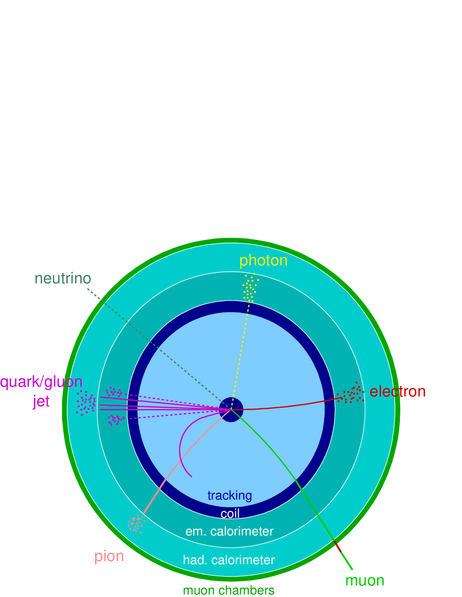
Figure 5.1: Patterns for identifying photon, electron, muon, charged hadron, and jet. Neutrino induces missing transverse energy.

5.1 Monte Carlo Simulation

Often we need to predict the output in the detector including the final reconstructed particles and the $\,/\!\!\!\!E_{T}$ of a particular interesting process and compare with data. Usually the phase space of an event of the $p\bar{p}$ collision is too complicated to be calculated analytically. In this case Monte Carlo (MC) simulation is used. It has become a powerful tool used in many research areas including high energy physics.

A well-known MC example is the Buffon’s Needle. It involves dropping a needle on a lined sheet of paper and determining the probability of the needle crossing one of the lines on the page. The remarkable result is that the probability is directly related to the value of the mathematical $\pi$. Suppose the length of the needle is one unit and the distance between the lines is also one unit. There are two variables, the angle $\theta$ at which the needle falls and the distance $D$ from the center of the needle to the closest line. $\theta$ can vary from 0^∘ to 180^∘ and is measured against a line parallel to the lines on the paper. $D$ can never be more than half the distance between the lines. The needle will hit the line if $D\leq\frac{1}{2}\sin\theta$. How often does this occur? The probability $\mathcal{P}$ is $2/\pi$ by integrating over $\theta$. With a computer, we can generate a large sample of random needle drops. The probability $\mathcal{P}$ can be simply taken as the number of hits divided by the number of drops, yielding $\pi=2/\mathcal{P}$.

Here we discuss the basic techniques of MC simulation. For a one-dimensional integral, we can choose $n$ numbers $x_{i}$ randomly with probability density uniform on the interval from $a$ to $b$, and for each $x_{i}$ evaluate the function $f(x_{i})$. The sum of these function values, divided by $n$, will converge to the expectation of the function $f$.

$$\int_{a}^{b}f(x)dx=(b-a)\langle f(x)\rangle\approx(b-a)\frac{1}{n}\sum_{i=1}^{n}f(x_{i})=(b-a)\overline{f_{n}}$$ (5.1)

The central limit theorem tells us that the sum of a large number of independent random variables is always normally distributed (i.e. a Gaussian distribution), no matter how the individual random variables are distributed. To understand this, we can test with uniformly distributed random variable $x_{1}$, $x_{2}$, $x_{3}$, $x_{4}$, (a) $x_{1}$ is a uniform distribution; (b) $x_{1}+x_{2}$ is a triangle distribution; (c) $x_{1}+x_{2}+x_{3}$ is already close to a Gaussian distribution; (d) $x_{1}+x_{2}+x_{3}+x_{4}$ is almost like the exact Gaussian distribution. Applying this theorem, we know the MC method is particularly useful as we can also calculate an error on the estimate by computing the standard deviation,

$$\langle f(x)\rangle=\overline{f_{n}}\pm\frac{\sigma_{n}}{\sqrt{n}}$$ (5.2)

where $\sigma_{n}=(\overline{f_{n}^{2}}-\overline{f_{n}}^{2})^{1/2}$ and $\overline{f_{n}^{2}}=\frac{1}{n}\sum_{i=1}^{n}f^{2}(x_{i})$. The convergence for numerically evaluating the integral goes as $1/\sqrt{n}$ with the number of function evaluation, $n$. And obviously if the distribution $f(x)$ is flatter, then the $\sigma_{n}$ is smaller for the same number of events in a sample generated. If there is a peak in the distribution such as the distribution of a resonance production, it is better to transform that variable to some other variable with a flatter distribution in order to converge faster.

The generalisation to multi-dimensional integrals $\int\!f(x,y,z,...)dxdydz...$ is straightforward. We can choose $n$ numbers of grid $(x,y,z,...)$ randomly with probability density uniform on the multi-dimensional phase space, and for each grid evaluate the function $f(x,y,z,...)$. The sum of these function values, divided by $n$, will converge to the expectation of the function $f$. A nice feature is that it will always converge as $1/\sqrt{n}$, even for very high dimensional integrals. This can make the performance of the MC method on multi-dimensional integrals very efficient.

In high energy physics, an event occurs with a probability in the phase space of the kinematic variables. A MC simulation generates a large number of random events according to the probability described by a model. With a large sample, we can get the predictions of the model by looking at the distributions of the kinematic variables and the derived variables, and the correlations among the variables. By confronting the predictions with real data, it is possible to tell if a model describes Nature correctly.

For this analysis, we use PYTHIA 6.215 program [21] with CTEQ5L parton density functions (PDF’s) [22] to generate the large samples of the processes of $p\bar{p}$ collision, such as $p\bar{p}\to\gamma^{*}/Z\to\tau\tau$, $p\bar{p}\to Z^{\prime}\to\tau\tau$, $p\bar{p}\to A\to\tau\tau$, and use TAUOLA 2.6 [23] to simulate tau decays. We use GEANT 3 [24] to simulate the response to the final particles in the CDF II detector.

5.2 Tau Identification

Tau leptons decay predominantly into charged and neutral pions and suffer from large backgrounds from jet production. Hadronic tau decays appear in the detector as narrow isolated jets. The most powerful cut to suppress the jet background is in fact isolation, requiring no other tracks or $\pi^{0}$s near the tau cone. To do this we define a signal cone and an isolation cone around the direction of the seed track (the track with the highest $p_{T}$) and then require that there is no track or $\pi^{0}$ between the signal cone and the isolation cone. This is shown in Fig. 5.2.

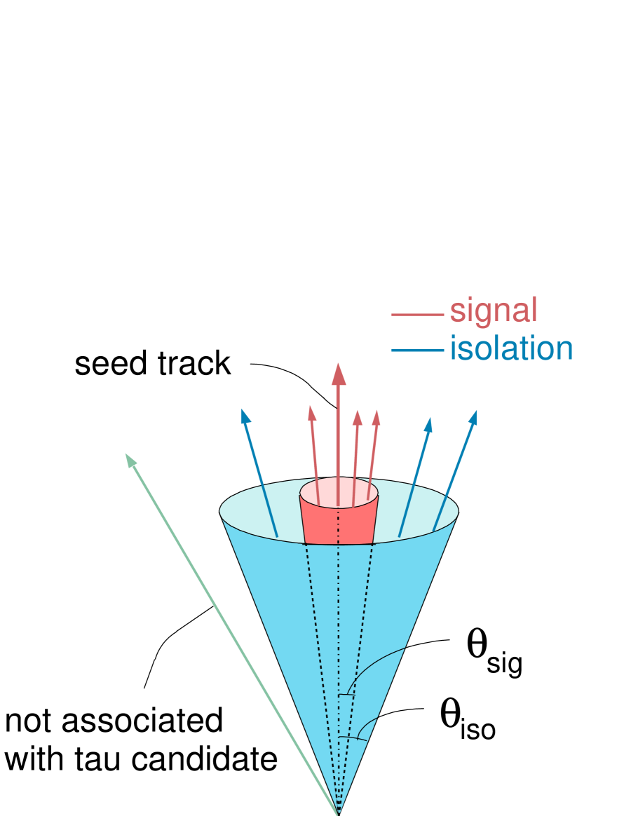
Figure 5.2: Illustration of tau isolation cone definitions.

5.2.1 Cone Size Definition

There are two useful cone size definitions. One is to construct a cone in $\Delta R$ defined below which has relativity invariance under a boost along the $z$-axis. The other is to construct a cone in three-dimensional separation angle, $\alpha$, which has geometry invariance. Below we discuss why $\Delta R$ is chosen as cone size definition for jet identification and why $\alpha$ is chosen as cone size definition for hadronic tau identification.

We start with the discussion on relativity invariance. For a particle under a boost $\beta=v/c$ along the $z$-axis and $\gamma=(1-\beta^{2})^{-1/2}$, its four-momentum $(p_{x},\;p_{y},\;p_{z},\;E)$ is transformed to

$$\left(\begin{array}[]{cccc}1&0&0&0\\ 0&1&0&0\\ 0&0&\gamma&\beta\gamma\\ 0&0&\beta\gamma&\gamma\end{array}\right)\left(\begin{array}[]{c}p_{x}\\ p_{y}\\ p_{z}\\ E\end{array}\right)=\left(\begin{array}[]{c}p_{x}\\ p_{y}\\ \gamma(p_{z}+\beta E)\\ \gamma(\beta p_{z}+E)\end{array}\right)$$ (5.3)

The $p_{x}$ and $p_{y}$ components in the transverse plane are not changed, while the $p_{z}$ component and the energy are changed. Rapidity is defined by

$$y=\frac{1}{2}\ln\frac{E+p_{z}}{E-p_{z}}$$ (5.4)

Using $\tanh^{-1}\beta=\frac{1}{2}\ln\frac{1+\beta}{1-\beta}$, it is easy to check that rapidity has a nice additive property under the boost along the $z$-axis,

$$y\to y+\tanh^{-1}\beta$$ (5.5)

For ultra-relativistic particle with $p\gg m$, we have $p_{z}/E\approx p_{z}/p=\cos\theta$. Using $\cos\theta=(1-\tan^{2}\frac{\theta}{2})/(1+\tan^{2}\frac{\theta}{2})$, the rapidity is well approximated by pseudorapidity $\eta$,

$$\eta=-\ln\tan\frac{\theta}{2}$$ (5.6)

Particles in a jet deposits energy in the calorimeter towers. For the traditional cone jet algorithm, we can call the tower with $E_{T}$ above a seed threshold as the seed (abbreviated as $s$), and the other towers with $E_{T}$ above a shoulder threshold as shoulders (abbreviated as $h$). To identify a jet, we can put the seed at the center and make a cone starting at a reconstructed interaction vertex point and around the seed to include the shoulders. Since the transverse components of a particle’s four-momentum are not changed under the unknown boost $\beta$ of the parton-parton system along the $z$-axis, $\phi$ is not changed. For an ultra-relativistic particle, $\eta$ is a good approximation of its rapidity. We have

$$\begin{array}[c]{llllllll}\phi_{s}&\to&\phi_{s},&&&\phi_{h}&\to&\phi_{h}\\ \eta_{s}&\to&\eta_{s}+\tanh^{-1}\beta,&&&\eta_{h}&\to&\eta_{h}+\tanh^{-1}\beta\end{array}$$ (5.7)

The separations in $\phi$ and $\eta$ are not changed under the unknown boost along the $z$-axis,

$$\begin{array}[c]{ccc}\Delta\phi=\phi_{h}-\phi_{s}&\to&\Delta\phi\\ \Delta\eta=\eta_{h}-\eta_{s}&\to&\Delta\eta\end{array}$$ (5.8)

Therefore the separation in $\Delta R$ which is constructed in the combination of $\Delta\phi$ and $\Delta\eta$ is not changed under the unknown boost along the $z$-axis,

$$\begin{array}[c]{ccc}\Delta R=\sqrt{(\Delta\eta)^{2}+(\Delta\phi)^{2}}&\to&\Delta R\end{array}$$ (5.9)

Given the $E_{T}$ and the configuration (shape) of a jet, whatever the magnitude of the boost along the $z$-axis of the parton-parton system is, or, equivalently, whatever the direction of the seed of the jet is, we can use the same cone to include or exclude a tower into the jet by calculating its separation in $\Delta R$ to the seed. Thus $\Delta R$ is a very useful shape variable for jet identification.

It also makes sence that there is a strong correlation between the two variables $E_{T}$ and $\Delta R$: a higher $E_{T}$ should give a smaller cone in $\Delta R$ to include all of the final particles, e.g. of a jet. It is very common that there are hundreds of final particles after a $p\bar{p}$ collision. The problem is that the energy of a jet in real data cannot be measured before a cone is actually constructed, otherwise there is no constraint to tell which tower should be included or excluded. Jet identification usually starts with a large and constant cone around a seed. The towers with significant energy in the cluster may or may not be contiguous. The energy of the jet is determined afterwards by summing up the energies of all of the towers in the cluster.

Now consider hadronic tau identification with a narrow cone and small number of final particles. The situation is quite different from jet identification. Since there are only a small amount of final particles, each final particle has significant energy. And since all of the final particles are in a narrow cone, they make a narrow and contiguous cluster with significant energy in each tower. This constraint of a narrow and contiguous cluster with significant energy in each tower tells us that we can determine energy first, and then construct a narrow cone to include or exclude charged particles reconstructed in the tracking system and/or neutral $\pi^{0}$s reconstructed in the shower maximum detector which is inside the electromagnetic calorimeter.

The question now is: is $\Delta R$ a good choice of cone size definition for hadronic tau identification?

A $\Delta R$ cone has a relativity invariance under a boost along the $z$-axis. However a $\Delta R$ cone does not have geometry invariance. What does a constant $\Delta R$ imply in geometry? The top plot of Fig. 5.3 shows three constant isolation annulus at different $\eta$ in a uniform $\eta$-$\phi$ space; the bottom plot shows the same three isolation annulus in a uniform $\theta$-$\phi$ space after using the function $\eta=-\ln\tan\frac{\theta}{2}$ to map $\eta$ slices to $\theta$ slices. In the central region, the isolation annulus is almost unchanged; outside the central region, they are severely squeezed, thus $\Delta\eta$ doesn’t have geometry invariance. $\Delta\phi$ doesn’t have geometry invariance either. Think of one step at the Equator of the Earth and another step at the North Pole of the Earth, the former is a tiny one in $\Delta\phi$ while the latter is a giant one in $\Delta\phi$. A constant $\Delta R$ cone with relativity invariance is not expected to be a constant cone with geometry invariance.

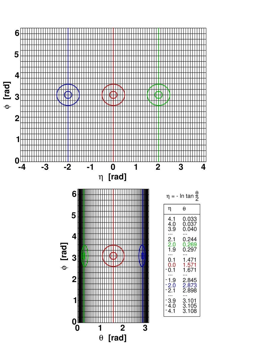
Figure 5.3: Lack of geometry invariance in $\Delta R$ cone.

Instead of $E_{T}$ and $\Delta R$, we can use energy $E$ and three-dimensional separation angle $\alpha$ to construct a cone for hadronic tau identification. There are two reasons.

First, consider a rotation of a solid cone; the geometry invariance of a three-dimensional separation angle $\alpha$ is easy to visualize. The unknown boost of the parton-parton system along the $z$-axis doesn’t affect the energy measurement of the hadronic tau identification at all. Under the known high energy boost, the final particles are flying together in a narrow cone. In one case the boost is to the central region, and in another case the boost is to somewhere forward or backward. Are these two cones geometrically invariant? The answer is yes.

Second, the correlation of $E$ and $\alpha$ is very strong. The case with the simplest phase space of final particles is calculable, see Appendix D. Comparing with a constant cone, a variable cone determined by this correlation can give extra power to suppress the jet background for hadronic tau identification. This is described by the “shrinking” cone algorithm for hadronic tau identification below.

5.2.2 The “Shrinking” Cone

As shown in Fig. 5.2, tau isolation cone, i.e., the outer cone, is a constant 30^∘ (0.525 rad) cone. For a particle with definite mass like tau, the bigger the energy, the smaller the separation angle of its decay daughters, hence a smaller signal cone which is the inner cone in Fig. 5.2.

The tau resonctruction algorithm [25] starts with a seed tower with $E_{T}>6$ GeV. It adds all of the adjacent shoulder towers with $E_{T}>1$ GeV to make a calorimeter cluster. The cluster is required to be narrow, i.e., the number of towers $\leq 6$. The visible energy, denoted as $E_{vis}$, of the final particles of tau haronic decays is measured by the energy of the calorimeter cluster, denoted as $E^{\tau\;obj}_{cluster}$. Then the algorithm asks a seed track with $p_{T}>4.5$ GeV/$c$ to match with the cluster. The matched seed track is a track with the highest $p_{T}$ in the neighbor of the calorimeter cluster. The tau signal cone is constructed around the direction of the seed track. The other tracks with $p_{T}>1$ GeV/$c$, and the $\pi^{0}$s with $p_{T}>1$ GeV/$c$ which are reconstructed by the strip and wire clusters in the CES detector, are included in the tau candidate if they are inside the tau signal cone. The size of the tau signal cone is determined by $E_{vis}$.

The phase space of tau hadronic decays is very complicated and the energy dependence of the signal cone cannot easily be calculated analytically. We use a large MC sample of $p\bar{p}\to Z\to\tau\tau$ to get this correlation.

The concept of tau shrinking signal cone at generation level (without underlying track or $\pi^{0}$) is shown in Fig. 5.4. The cone starts out at a constant 10^∘, and then, if the quantity (5 rad)/$E_{vis}$ is less than 10^∘ we use this angle, unless it is less than 50 mrad.

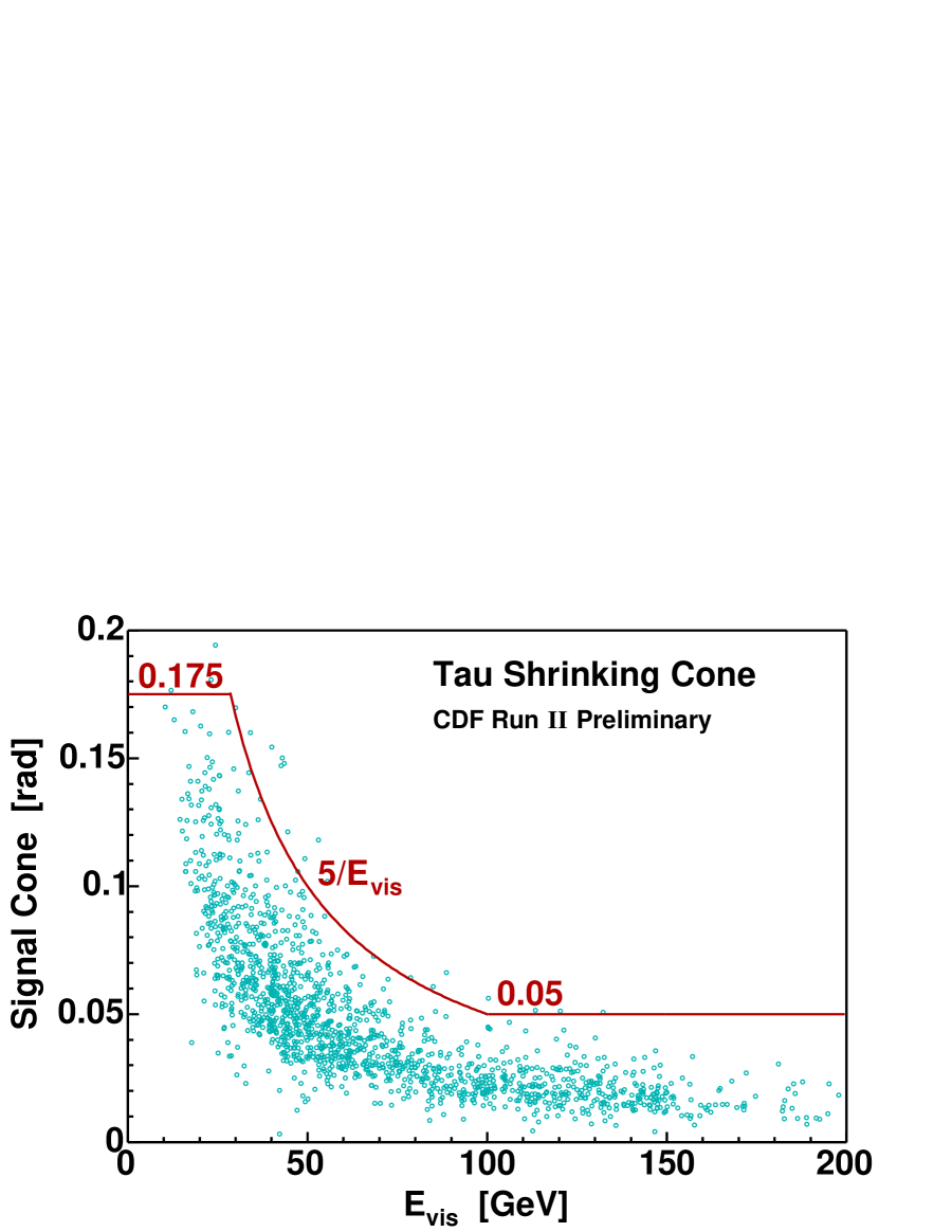
Figure 5.4: Distribution of maximum angle between tau decay products and tau seed track as a function of tau visible decay product energy. The red line indicates the half-width of the ”shrinking” tau signal cone as a function of energy.

For reconstructed tracks a cone defined as that shown in Fig. 5.4 is efficient and selective against jet backgrounds. However, for $\pi^{0}$s, the reconstructed angle can, at large visible energies, be larger than 50 mrad. Thus we relax the minimum to 100 mrad. With underlying track or $\pi^{0}$, the shrinking cone is shown in the left two plots of Fig. 5.5. Inside the tau isolation cone (the outer 0.525 rad cone), the separation angle between the farthest track/$\pi^{0}$ and the seed track is ploted. A tau object between the tau isolation cone and the shrinking signal cone is non-isolated and will be removed by isolation cut. The right two plots of Fig. 5.5 show how the shrinking cone looks when applied to jets reconstructed as tau objects. Comparing with a constant signal cone, the shrinking signal cone, a natural consequence of the tau’s relativistic boost, dramatically helps to reduce jet background in the high mass search.

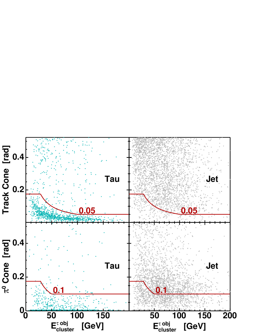
Figure 5.5: Due to different reconstruction resolutions, the minimum cone sizes of the “shrinking” cone for track and $\pi^{0}$ are 0.05 and 0.1 radian, respectively, shown in the left two plots for tau. The right two plots show how the “shrinking” cone looks when applied to jets reconstructed as tau objects.

5.2.3 Tau Identification Cuts

Now we can put the seed track in the center of the cone and include in the tau candidate all tracks and $\pi^{0}$s whose direction is within the “shrinking” signal cone. Table 5.1 shows the list of tau identification cuts using the information about calorimeter cluster, seed track, shoulder tracks/$\pi^{0}$s of the tau candidate. The $p_{T}$(tracks + $\pi^{0}$s) threshold is not listed because it is not an identification cut and it should be chosen by looking at the trigger cuts applied and by comparing tau identification efficiency with the jet$\to\tau$ misidentification rate. We do not cut on charge because there is an ambiguity in the charge for high $p_{T}$ tracks; we do not cut on track multiplicity either because we will check track multiplicity to see hadronic tau signature.

Variable	Cut	Note	Denominator
$|\eta_{det}|$	$<$1	central calorimeter
$|z_{loc}|$	9$<|z_{loc}|<$230 cm	fiducial ShowerMax
$\xi$	$>$0.2	electron removal	$D_{\xi}$
$p_{T}^{seed}$	$>$6 GeV/$c$	seed track $p_{T}$
10∘ track isolation	constant cone	weaker than shrinking	$D_{trkIso10Deg}$
m(tracks)	$<$1.8 GeV/$c^{2}$	weaker than vis. mass	$D_{trkMass}$
$|z_{0}|$	$<$60 cm	vertex $z$
$|d_{0}|$	$<$0.2 cm	impact prameter
seed track ax. seg.	$\geq$3$\times$7	COT axial segments
seed track st. seg.	$\geq$3$\times$7	COT stereo segments
track isolation	shrinking track cone	shoulder tracks
$\pi^{0}$ isolation	shrinking $\pi^{0}$ cone	shoulder $\pi^{0}$s
$E^{em}_{iso}$	$<$2 GeV	EM cal. isolation
m(tracks + $\pi^{0}$s)	$<$1.8 GeV/$c^{2}$	visible mass	Numerator

Table 5.1: Tau identification cuts.

Electron Removal

Using the requirements discussed above, electrons can be reconstructed as hadronic tau objects if they have a narrow calorimeter cluster and a high $p_{T}$ seed track. To remove electrons we demand that the tau be consistent with having only pions in the final state. We define the variable $\xi$ as

$$\xi\equiv\frac{E}{p}(1-\frac{E_{em}}{E})=\frac{E_{had}}{p}$$ (5.10)

Fig. 5.6 shows the tau object EM fraction ($E_{em}/E$) versus E/p. The top plot is for hadronic taus reconstructed as tau objects, and the bottom plot is for electrons reconstructed as tau objects. For an ideal hadronic tau and a perfect calorimeter, $\xi$ = 1. For an ideal electron, $\xi$ = 0. However, the calorimeter is not perfect and there can be a large background from $Z\to ee$ events. To remove this background we use a very tight cut, $\xi>$ 0.2. The remaining background is discussed below.

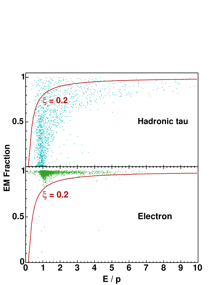
Figure 5.6: Distributions of EM fraction ($E_{em}/E$) vs. $E/p$ for hadronic tau and electron. $\xi>0.2$ is used to remove electron.

EM Calorimeter Isolation

The motivation for the EM calorimeter isolation cut is due to $\pi^{0}$ reconstruction inefficiency, for example, some CES clusters are not reconstructed as $\pi^{0}$s if a track is nearby. This affects the power of the $\pi^{0}$ isolation requirement. We add an EM calorimeter isolation cut to deal with the remaining jet background. We calculate the EM energy in a $\Delta R=0.4$ cone around the seed track, summing over all EM towers which are not members of the tau cluster. Here $\Delta R$ is used to calculate the distance between the centroid of a calorimeter tower and the seed track because the calorimeter tower segmentation is fixed in $\eta\times\phi$ space, namely $0.11\times 15^{\circ}$ around the central region. Since the EM calorimeter isolation cut is strongly correlated with other isolation cuts, its marginal distribution is shown in Fig. 5.7. The EM cal. isolation energy versus cluster energy plots show that we do not need to use a relative (fractional) cut, which is necessary if for high energy tau objects there is significant energy leakage outside tau cluster. We instead choose an abosolute cut, $E^{em}_{iso}<2$ GeV.

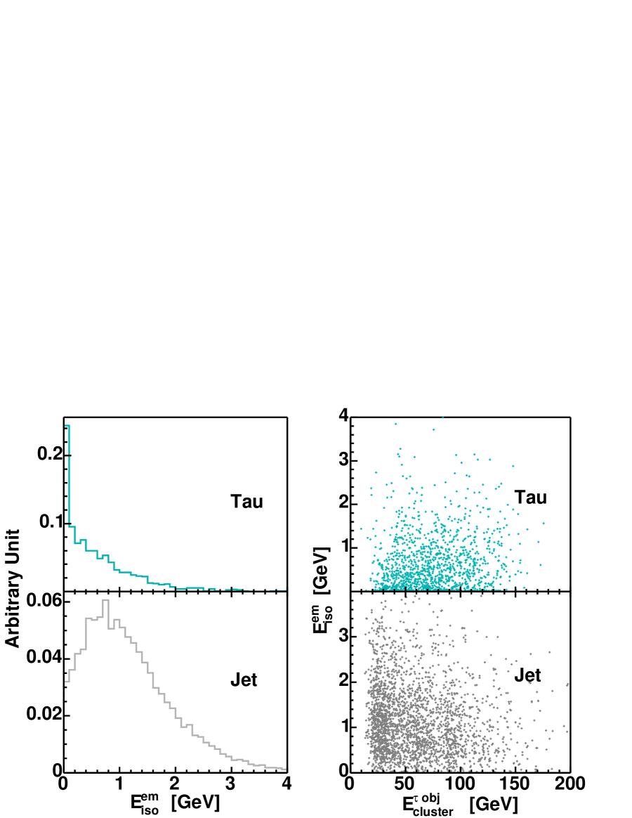
Figure 5.7: Disbutions of EM calorimeter isolation for tau and jet, and distributions of EM calorimeter isolation vs. energy of reconstructed tau object for tau and jet.

Object Uniqueness

Though not listed in the summary table of tau identification cuts, we note that all reconstructed objects in the event are required to be unique. Thus we only apply the tau identification cuts to objects not already reconstructed as a photon, electron, or muon. In practice, we require that a tau object be 30^∘ away from any identified photon, electron, or muon.

Denominators

For various subsequent studies presented here we will use specific subsets of the tau identification cuts listed in the summary table. The cuts are in cumulative order which is important for calculating rates and efficiencies. There are three different denominators in Table 5.1 corresponding to three different relative rates, which will be applied on different data samples with consistent denominators later.

5.2.4 Tau Identification Efficiency

Table 5.2 shows the procedure to measure the tau identification efficiency, using different samples. For all of the generated taus, we pick those taus decaying hadronically, and consider the central ones in the pseudorapidity range $|\eta|<1$ which are able to be reconstructed as tau object, called CdfTau in the table. We require the seed track of the generated tau to match with the seed track of a reconstructed tau object within 0.2 radian. Then we apply the tau identification cuts on the reconstructed tau objects and calculate tau identification efficiency.

Fig. 5.8 shows the absolute tau identification efficiency, which includes the effects of both reconstruction and identification, vs. tau visible energy, using the $Z^{\prime}$ sample which has a lot of high energy taus.

5.2.5 Jet$\to\tau$ Misidentification Rate

Table 5.3 shows the procedure to measure the jet$\to\tau$ misidentification rate, using four different jet samples called JET20, JET50, JET70, and JET100 samples collected with different trigger thesholds. The L1 tower $E_{T}$, L2 cluster $E_{T}$ and L3 jet $E_{T}$ trigger thresholds in the unit of GeV for a triggered jet in each jet sample are

• JET20: 5, 15, 20

• JET50: 5, 40, 50

• JET70: 10, 60, 70

• JET100: 10, 90, 100

We use the central jets with $|\eta|<1$ which may be reconstructed as tau object, called CdfTau in the table. We require the central jet to match with a reconstructed tau object by requiring that they share the seed tower of the reconstructed tau object. Then we apply the tau identification cuts on the reconstructed tau objects and calculate jet$\to\tau$ misidentification rate.

Fig. 5.9 shows the absolute jet$\to\tau$ misidentification rate, which includes the effects of both reconstruction and identification, vs. jet cluster energy, using JET50 sample.

Procedure	$W\to\tau\nu$	$Z\to\tau\tau$	$Z^{\prime}\to\tau\tau$	Denominator
event	491513	492000	1200000
tau hadronic	319357	637889	1554159
tau central	150984	275330	898102	$D_{absolute}$
tau match CdfTau	86325	165495	800262	$D_{CdfTau}$
$|\eta_{det}|<1$	85899	164722	797705
$9<|z_{loc}|<230$ cm	82240	157748	758403
$\xi>0.2$	65854	127403	663845	$D_{\xi}$
$p_{T}^{seed}>6$ GeV/$c$	60960	119451	651328
10∘ track isolation	50309	98717	540485	$D_{trkIso10Deg}$
m(tracks) $<1.8$ GeV/$c^{2}$	50141	98355	532190	$D_{trkMass}$
$|z_{0}|<60$ cm	48659	95333	515239
$|d_{0}|<0.2$ cm	47975	93969	506453
seed track ax. seg. $\geq 3\times 7$	47822	93657	501965
seed track st. seg. $\geq 3\times 7$	47312	92666	494069
track isolation (shrinking)	47112	92042	475017
$\pi^{0}$ isolation (shrinking)	45687	89148	451129
$E^{em}_{iso}<2$ GeV	43981	85910	428641
m(tracks + $\pi^{0}$s) $<1.8$ GeV/$c^{2}$	43155	84218	404105	Numerator

Table 5.2: Number of events for tau identification efficiency measurement.

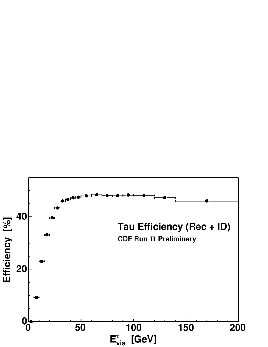
Figure 5.8: Tau identification efficiency vs. tau visible energy.

Procedure	JET20	JET50	JET70	JET100	Denominator
event	7696880	1951396	910618	1137840
event goodrun	4309784	1213104	556961	697231
jet non-triggered	21957203	6071557	2641643	2935801
jet central	8214991	2480232	1127376	1321840	$D_{absolute}$
jet match CdfTau	653680	425086	189148	201530	$D_{CdfTau}$
$|\eta_{det}|<1$	643190	416560	184996	196651
$9<|z_{loc}|<230$ cm	611401	393222	174474	184980
$\xi>0.2$	521326	354504	159320	169441	$D_{\xi}$
$p_{T}^{seed}>6$ GeV/$c$	414966	315384	145124	156391
10∘ track isolation	105846	74425	36231	42727	$D_{trkIso10Deg}$
m(tracks) $<1.8$ GeV/$c^{2}$	92475	63616	31865	37709	$D_{trkMass}$
$|z_{0}|<60$ cm	85754	56951	28146	32747
$|d_{0}|<0.2$ cm	79889	51829	25391	28994
seed track ax. seg. $\geq 3\times 7$	78500	50043	24293	27474
seed track st. seg. $\geq 3\times 7$	71926	42754	20058	21828
track isolation (shrinking)	64489	20679	7475	7293
$\pi^{0}$ isolation (shrinking)	50886	13910	5025	4965
$E^{em}_{iso}<2$ GeV	41749	11132	4073	3969
m(tracks + $\pi^{0}$s) $<1.8$ GeV/$c^{2}$	35314	7965	2879	2792	Numerator

Table 5.3: Number of events for jet$\to\tau$ misidentification rate measurement.

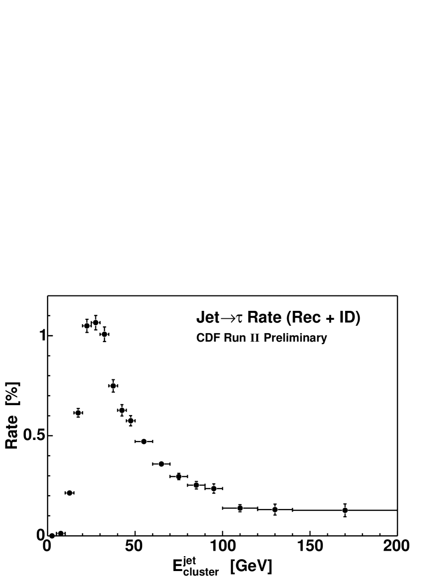
Figure 5.9: Jet$\to\tau$ misidentification rate vs. energy, using JET50 sample.

Discrepancies

To try to minimize trigger bias, we use non-triggered jet only. Based on the L1 tower $E_{T}$, L2 cluster $E_{T}$ and L3 jet $E_{T}$ trigger thresholds in each sample, we find all of the jets which can satisfy the trigger requirements. The choice of the triggered jets in an event in the case of zero, one or more than one jet satisfying trigger requirements are

• If zero, throw away the event

• If only one, choose that jet

• If more than one, do not choose any as triggered

Non-triggered jets are just the jets not chosen as the triggered jet. Even after trying to minimize trigger bias by using non-triggered jet only, there are still discrepancies among jet$\to\tau$ misidentification rates obtained from different jet samples, shown in Fig. 5.10.

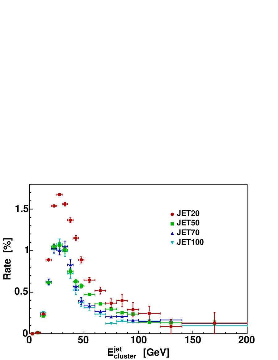
Figure 5.10: Discrepancies of jet$\to\tau$ misidentification rates in JET samples.

Two-Dimensional Parametrization

There is no doubt that the jet$\to\tau$ misidentification rate has a very strong dependence on energy because the tau isolation annulus is a function of energy. To resolve the discrepancies among the jet$\to\tau$ rates, we add another parameter to make a two-dimensional parametrization. The second parameter should not be correlated strongly with energy, otherwise adding another parameter is meaningless. Given the final particles, the transverse size of a jet depends on its boost: jets with a bigger boost have smaller size and smaller size jets have higher probability to survive tau identification. The relativistic boost $\gamma$ is

$$\gamma=\frac{E}{m}$$ (5.11)

where $E$ is the energy of the jet which can be measured by its cluster energy in calorimeter, and $m$ is the invariant mass of its final particles. The mass $m$ is not easy to measure because some of the final particles can be neutral and leave no track in tracking system. We use cluster mass, which treats each tower in the cluster as a massless photon and sums up the photons, as an approximation of $m$. The cluster mass has a strong correlation with energy, while the cluster boost does not. This is shown in Fig. 5.12. We choose cluster boost as the second parameter.

In the one-dimensional jet$\to\tau$ misidentification rate what we see is the average over all of the bins of cluster boost. Given the energy of a jet, the average cluster boost is different in JET samples, shown in Fig. 5.12.

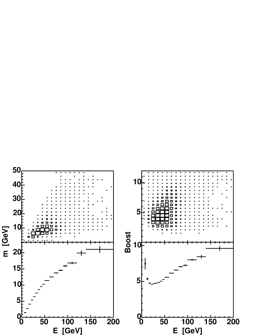
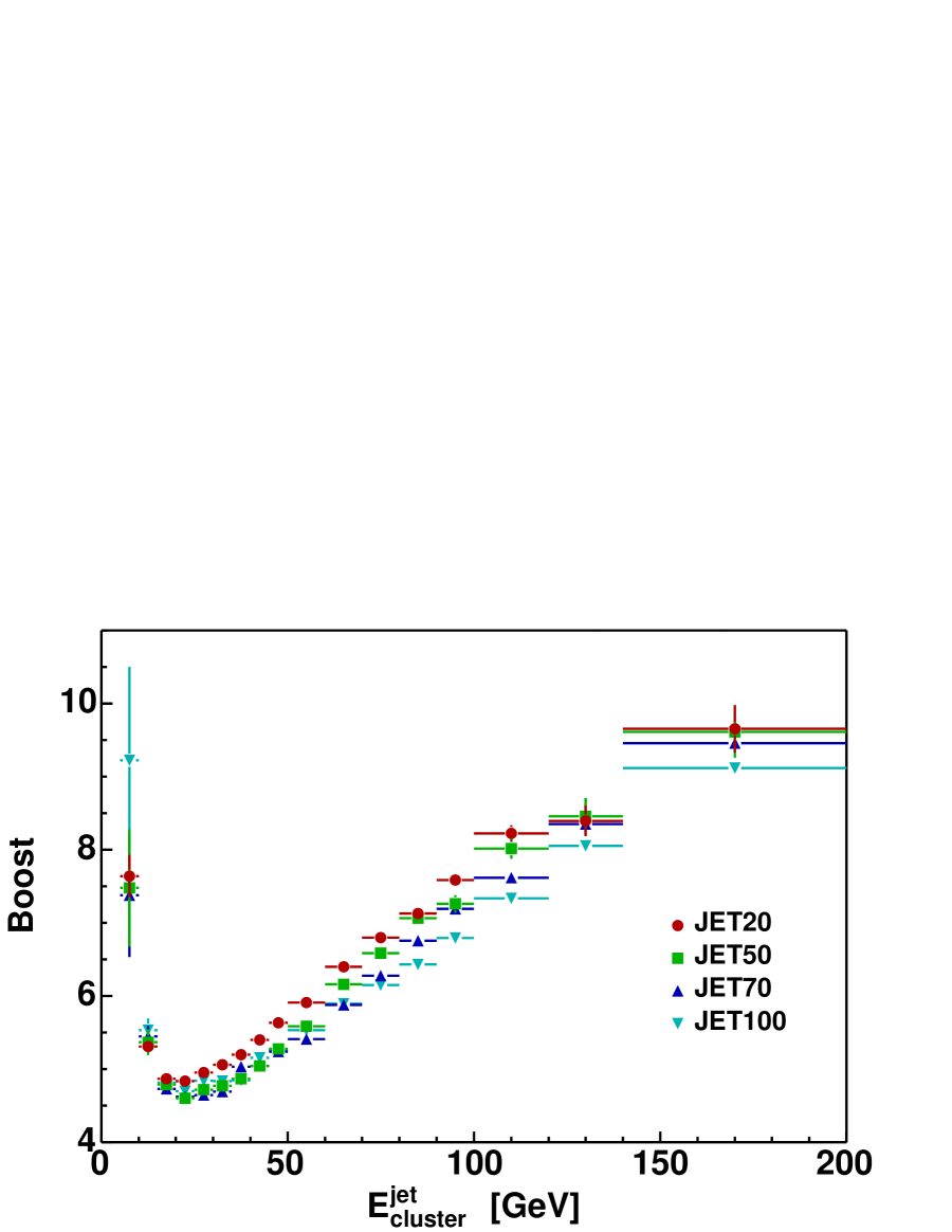
Figure 5.11: Distributions of jet cluster: mass vs. energy, and boost vs. energy, in JET50 sample.

Figure 5.12: Profiles of jet cluster boost vs. cluster energy in JET samples.

Now we plot the jet$\to\tau$ misidentification rate vs. energy, in each boost slice, shown in Fig. 5.13. With the new two-dimensional parametrization, the overall discrepancy drops down to about 20%. Since the discrepancies are not totally resolved, there are other unknown effects.

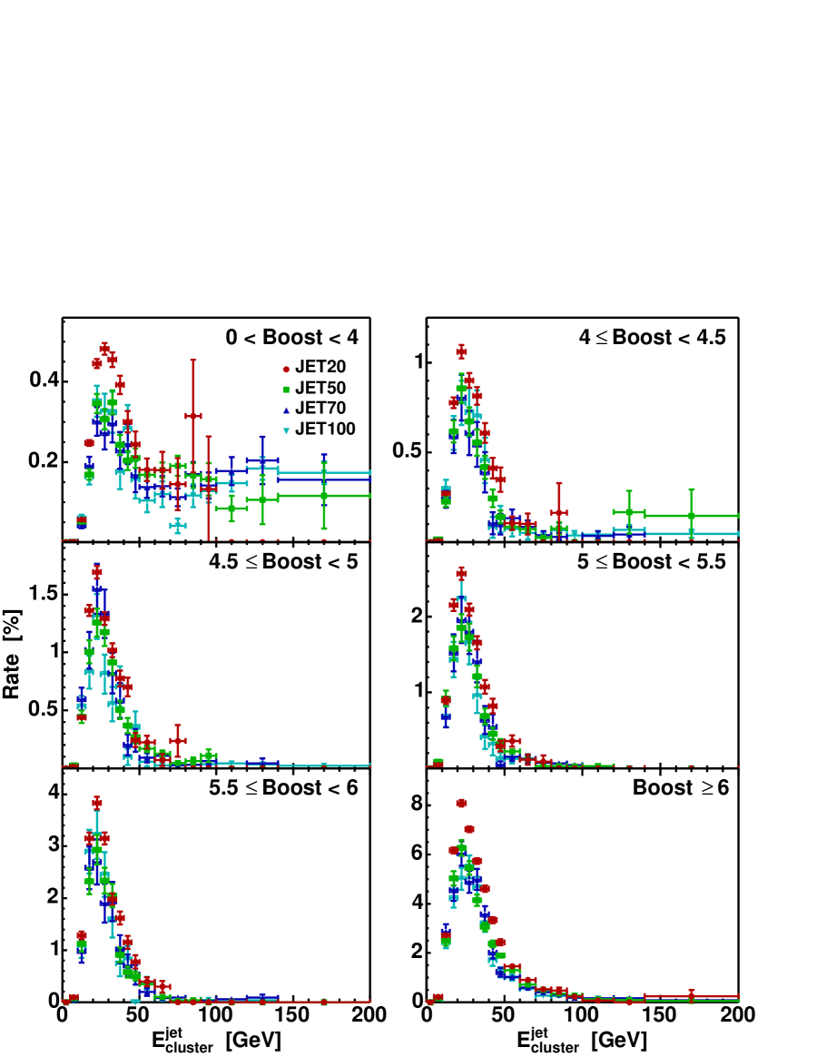
Figure 5.13: Jet$\to\tau$ misidentification rate vs. energy in JET samples and in jet cluster boost slices.

5.2.6 Jet$\to\tau$ Background Estimate

After applying the full set of tau identification cuts, there will be some jet background left because of the huge production rate of jets in $p\bar{p}$ collisions. The jet$\to\tau$ misidentification rate and tau identification efficiency are very useful for estimating jet background.

To estimate the jet background, the starting point is not jets, or tau candiates, but tau candidates with at least electron removal, with a very tight $\xi>$ 0.2 cut applied. Muons usually cannot have enough energy to make a tau cluster in the calorimeter. We have two general equations,

Before full tau ID: $$\tilde{N}=\tilde{N}^{\tau}+\tilde{N}^{jet}$$ (5.12)

After full tau ID: $$N=N^{\tau}+N^{jet}=e\tilde{N}^{\tau}+f\tilde{N}^{jet}$$ (5.13)

where $f$ is jet$\to\tau$ misidentification rate and $e$ is tau identification efficiency. Both are relative in a sense that they are relative to the starting point chosen as “Before full tau ID”. The solution is

$$N^{jet}=\frac{f}{e-f}(e\tilde{N}-N).$$ (5.14)

Fig. 5.14 is a demonstration of picking one bin and using the formula to estimate jet background. This is only an example because the parametrization of the relative rates is a one-dimensional function of energy. For the jet$\to\tau$ misidentification rate there is a better parametrization, i.e., the two-dimensional function of energy and boost.

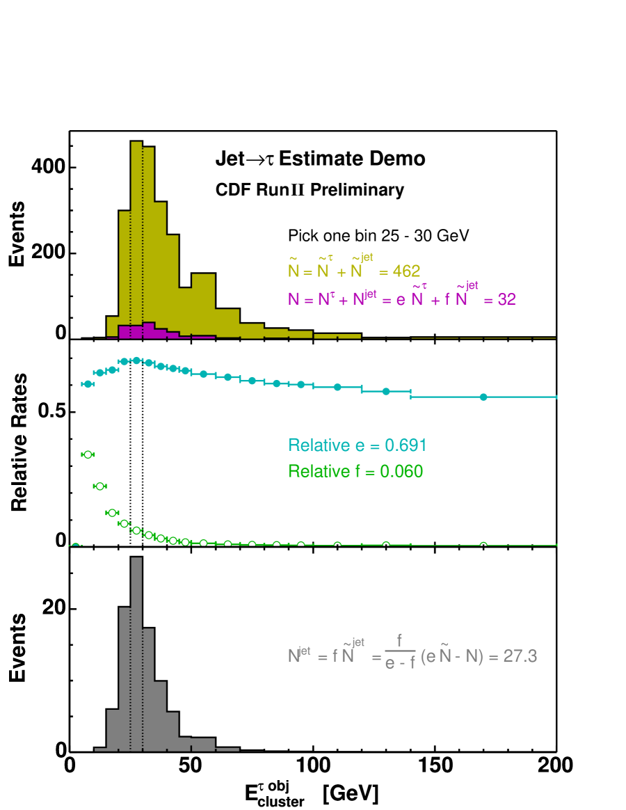
Figure 5.14: Demonstration of estimating jet$\to\tau$ misidentification.

Implementation

The actual implementation is done on an event-by-event basis. For a tau object in an event under consideration, the knowns are: $\tilde{N}$ = 1, $e$, $f$ and whether this tau object passes the full set of the tau identification cuts. If it does, $N$ = 1; otherwise, $N$ = 0. For the two cases, the weight to be a jet is estimated as

If not passing the full tau ID cuts: $$\omega^{jet}=\frac{f}{e-f}(e-0)$$ (5.15)

If passing the full tau ID cuts: $$\omega^{jet}=\frac{f}{e-f}(e-1)$$ (5.16)

In terms of coding, it means the rest of full tau identification cuts are replaced by the weight $\omega^{jet}$. We sum up the weights of all the events in the sample, and get the jet background estimate $N^{jet}$,

$$N^{jet}=\sum\omega^{jet}$$ (5.17)

Special Case

This method actually needs both the jet$\to\tau$ misidentification rate $f$ and the tau identification efficiency $e$. The main idea is to remove the contribution from any real tau signal in jet background estimate.

The special case is that if we start with a jet-dominated sample and $f$ is much smaller than $e$, then we can suppress signal by replacing tau identification cuts with the jet$\to\tau$ misidentification rate,

$$N^{jet}=f\tilde{N}^{jet}\approx f\tilde{N}\;\;\;\;(f\ll e)$$ (5.18)

5.3 Tau Scale Factor Using $W\to\tau\nu$

In this section, we apply tau identification cuts to select hadronic taus in $W\to\tau\nu$ events, estimate jet$\to\tau$ misidentification background, study tau identification scale factor and compare tau distributions in data and MC simulation.

5.3.1 Data/MC Scale Factor

The scale factor for a set of cuts quantifies and corrects for the difference between data and MC simulation. It should be multiplied on MC to get the scaled efficiency consistent with the efficiency in data. Fig. 5.15 shows lepton flow in data and in MC, and lepton data/MC scale factors.

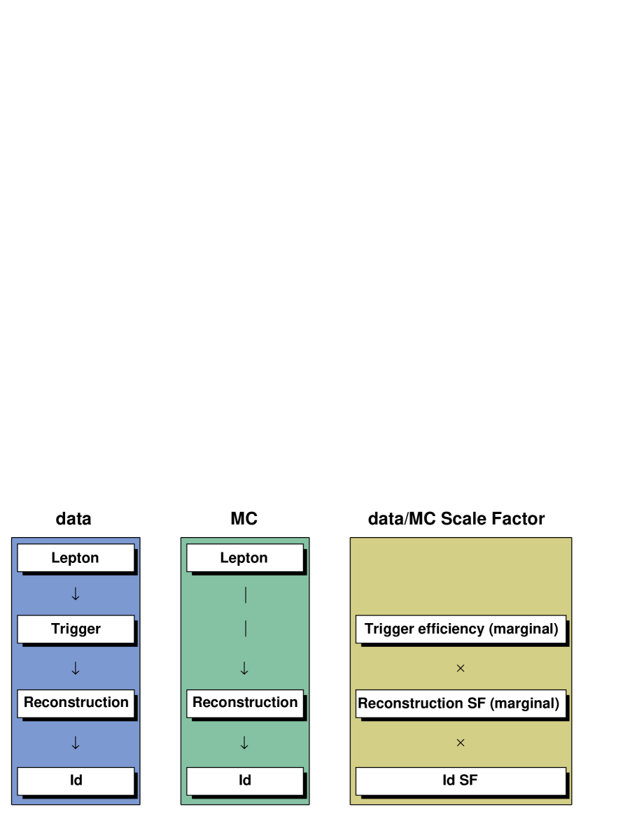
Figure 5.15: Lepton in data and in MC, and lepton data/MC scale factors.

Ratio of Efficiencies

A data/MC scale factor is defined as the ratio of efficiencies,

$$f_{data/MC}=\frac{\epsilon_{data}}{\epsilon_{MC}}$$ (5.19)

where $\epsilon_{MC}$ is the efficiency in MC which is straightforward to obtain because the MC simulation has the true information of particle identity, and $\epsilon_{data}$ is the efficiency in data, which can be a challenge to measure.

In the electron or muon case, we can use electron or muon pairs from the Z boson peak, which gives us a pure sample with negligible background in real data. This is so reliable that we can use it as “standard candle” to calibrate detector and even measure luminosity. We select one leg to satisfy the trigger requirements in data, and ask whether the second leg passes the set of cuts, and thereby get the efficiency in data.

Ratio of Numbers

Due to the missing energy from the neutrino in tau decays, the tau pair mass at the Z boson peak is severely broadened. Instead, we will use $W\to\tau\nu$ to select a relatively clean tau sample. There is no second leg to get efficiency data/MC. We use the method of absolute number data/MC,

$$f_{data/MC}=\frac{n_{data}}{n_{MC}}$$ (5.20)

where $n_{MC}$ is the absolute number of $W\to\tau\nu$ events in MC normalized to the luminosity of data, and $n_{data}$ is the number of $W\to\tau\nu$ events observed in the data after subtracting backgrounds.

5.3.2 $W\to\tau\nu$ Selection

We select $W\to\tau\nu$ events by using a data sample from the TAU_MET trigger which requires:

• level 1 trigger (L1) $\,/\!\!\!\!E_{T}>$ 25 GeV

• level 3 trigger (L3) tau $E_{T}>$ 20 GeV

where (a) L1 $\,/\!\!\!\!E_{T}$ is based on a tower threshold of 1 GeV for a fast calculation; (b) for L3 tau, the cuts $|\eta_{det}|<$ 1, 10^∘ track isolation and m(tracks) $<$ 2 GeV/$c^{2}$ are applied in the trigger.

The top plot of Fig. 5.16 shows that the integrated luminosity of the good runs is 72 $\pm$ 4 pb^-1, and the bottom plot shows the L3 cross section is reasonablly flat (no sudden drop to zero), thus all of the good runs are present in the data file.

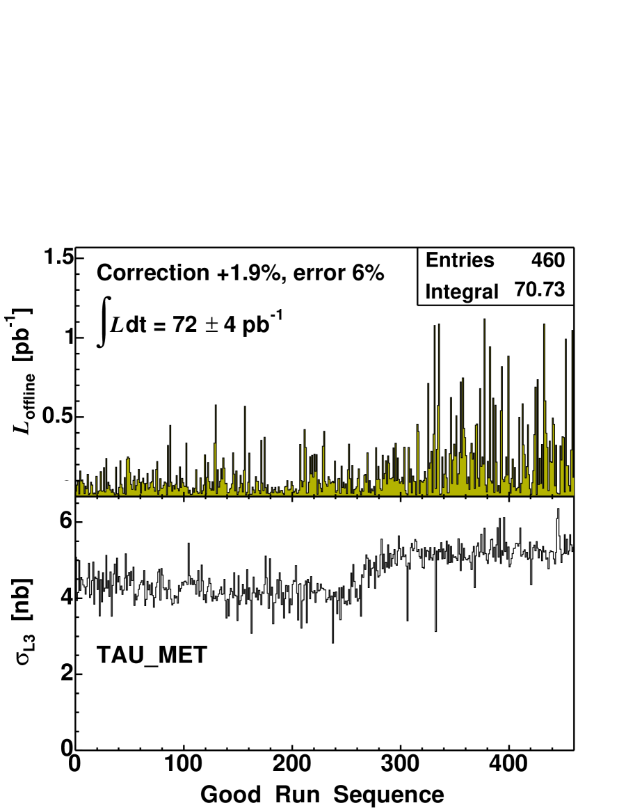
Figure 5.16: Distributions of offline luminosity vs. good run sequence and L3 cross section vs. good run sequence, in the data sample from TAU_MET trigger.

The offline selection cuts are:

• Monojet

• $\,/\!\!\!\!E_{T}>$ 30 GeV

• Tau $p_{T}$(tracks + $\pi^{0}$s) $>$ 25 GeV/$c$

where (a) monojet selection requires one central cone 0.7 jet with $|\eta_{det}|<$ 1 and $E_{T}>$ 25 GeV, no other jets with $E_{T}>$ 5 GeV anywhere; (b) offline $\,/\!\!\!\!E_{T}$ is obtained from the vector sum of $E_{T}$ for towers with $E_{T}>0.1$ GeV; (c) in addition to tau $p_{T}$ threshold, the whole set of tau identification cuts under study will be applied on the offline tau candidates.

The monojet cut dramatically helps clean up the data sample. But, to get the estimated $n_{MC}$ of $W\to\tau\nu$ events, we need to study the monojet cut and the L1 $\,/\!\!\!\!E_{T}>$ 25 GeV trigger efficiency for monojet-type events.

Monojet Selection

The monojet selection essentially requires there is no other underlying jet with $E_{T}>$ 5 GeV. We select $Z\to\mu\mu$ events, count the number of cone 0.7 jets with $E_{T}>$ 5 GeV, no $\eta$ cut, and 0.7 radian in $\Delta$R away from muons.

The $Z\to\mu\mu$ selection cuts are: (a) cosmic veto [26], (b) one tight muon and one track with $p_{T}>$ 20 GeV/$c$, (c) opposite charges, (d) track $|z_{0}(1)-z_{0}(2)|<$ 4 cm, and (e) $80<m_{\mu\mu}<100$ GeV/$c^{2}$. We require one tight muon and one track, instead of two tight muons to get higher statistics. The track is required to be of minimum ionisation particle (MIP) type. Both the tight muon and the track requires tau-like track isolation which is to mimic the isolated tau in $W\to\tau\nu$ events.

We use a data sample from a trigger designed to select “muon plus track” events which have $\mu$ with $p_{T}>8$ GeV/$c$ plus another charged track with $p_{T}>5$ GeV/$c$. We select 5799 events with negligible background which is confirmed by the negligible number of same-charge muon pair events. There are 2152 events in the zero jet bin. The fraction of zero jet events in the data is 2152/5799 = 0.371.

We use about 500K MC events. 46297 events survived after the same selection cuts as in data. There are 20149 events in the zero jet bin. The fraction of zero jet events in the MC is 20149/46297 = 0.435.

The number of jets distribution in data and in MC are shown in Fig. 5.18. So $W\to\tau\nu$ monojet data/MC scale factor is

$$f^{monojet}_{data/MC}=\frac{2152/5799}{20149/46297}=\frac{0.371}{0.435}=0.85\pm 0.02$$ (5.21)

The uncertainty is statistical only.

L1 $\,/\!\!\!\!E_{T}>$ 25 GeV

The TAU_MET trigger triggers directly on tau objects, and so there is no marginal trigger efficiency from TAU side. But there is marginal trigger efficiency from MET side: L1 $\,/\!\!\!\!E_{T}$ uses a 1 GeV tower threshold, and offline $\,/\!\!\!\!E_{T}$ uses a 0.1 GeV tower threshold.

We use JET20 data to study this trigger efficiency. The event topology is monojet-like, since here that is what we are interested in. The L1 $\,/\!\!\!\!E_{T}>$ 25 GeV trigger efficiency vs offline $\,/\!\!\!\!E_{T}$ for monojet event is shown in Fig. 5.18. It is a slow turn-on due to a large tower threshold. An offline $\,/\!\!\!\!E_{T}>$ 30 GeV cut is not fully efficient.

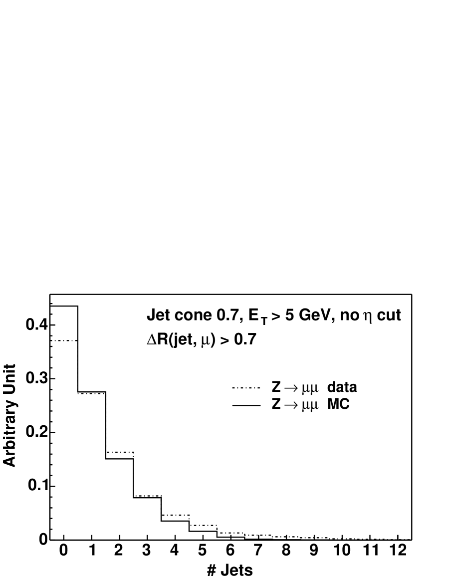
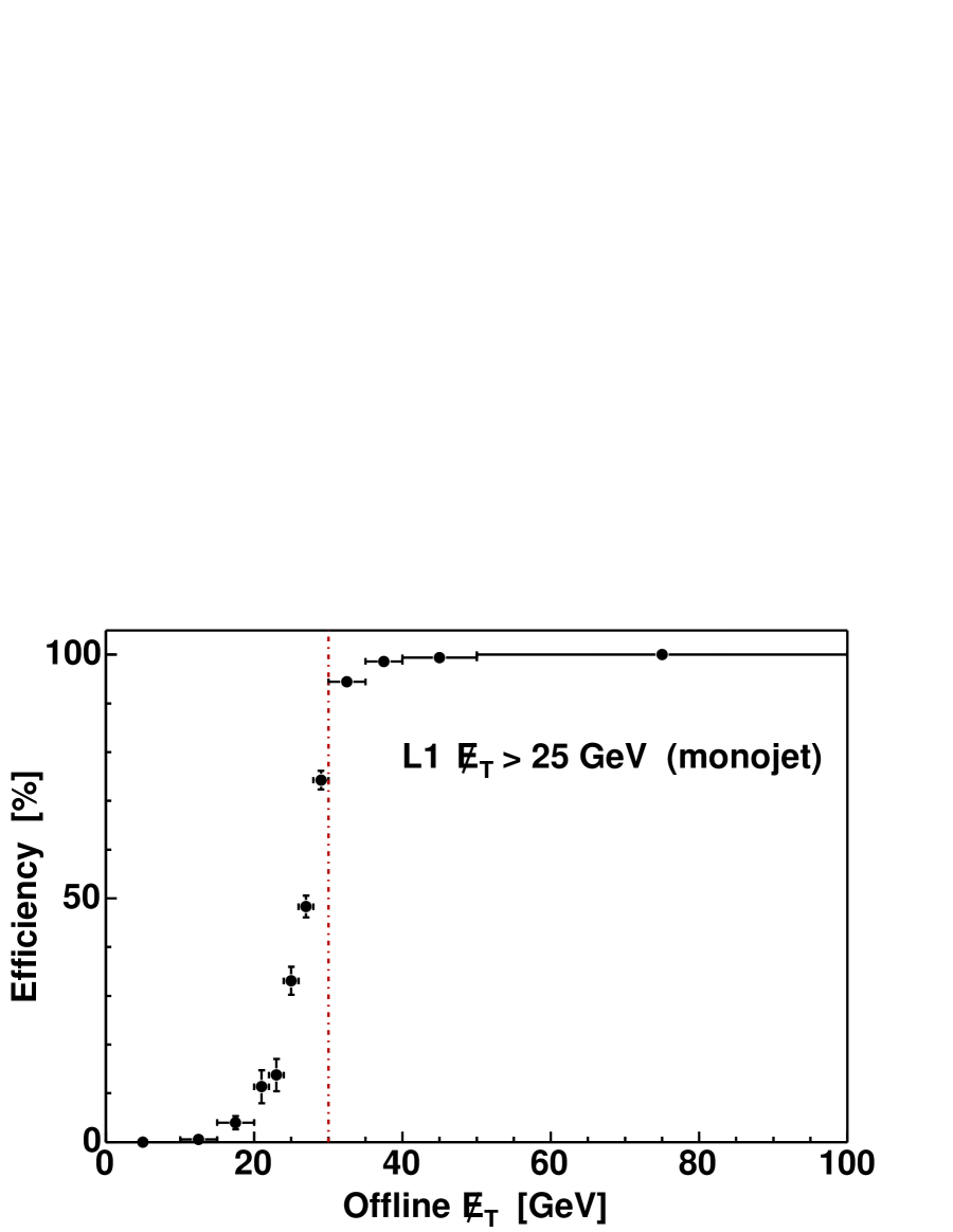
Figure 5.17: Distributions of the number of jets in $Z\to\mu\mu$ data and MC.

Figure 5.18: L1 $\,/\!\!\!\!E_{T}>$ 25 GeV trigger efficiency vs. offline $\,/\!\!\!\!E_{T}$ for monojet event.

5.3.3 Tau Scale Factor

After all of the above, we count the absolute number of $W\to\tau\nu$ events $n_{data}$ and $n_{MC}$ for total integrated luminosity 72 pb^-1. Their ratio will be the tau scale factor.

• To get $n_{data}$, we will use the data sample from the TAU_MET trigger. We apply the offline cuts to get the observed number of $W\to\tau\nu$ candidates, and subtract various backgrounds.

• To get $n_{MC}$, we will use $W\to\tau\nu$ MC simulation. We apply the offline cuts, multiply the number of accepted events by the monojet scale factor and the trigger efficiency, and normalize to 72 pb^-1.

The main source of backgrounds are $W\to e\nu$, $W\to\mu\nu$, $Z/\gamma^{*}\to\tau\tau$, and jet background.

We will use MC simulation to get $W\to e\nu$, $W\to\mu\nu$, and $Z/\gamma^{*}\to\tau\tau$ backgrounds. We apply the offline cuts, multiply the number of accepted events by the monojet scale factor and the trigger efficiency, and normalize to 72 pb^-1. For the normalization in MC, $\sigma\cdot B(W\to l\nu)$ is 2700 pb [20], and $\sigma\cdot B(Z/\gamma^{*}\to ll)$ is 326 pb with $m_{Z/\gamma^{*}}>30$ GeV/$c^{2}$, which is obtained from the measured value 250 pb [20] at the Z boson mass peak with $66<m_{Z/\gamma^{*}}<116$ GeV/$c^{2}$ and normalizing the $Z/\gamma^{*}\to ll$ mass spectrum generated by PYTHIA.

The jet background will be estimated directly from the data by applying the relative jet$\to\tau$ misidentification rate and the relative tau identification efficiency. Since the cuts $|\eta_{det}|<1$, 10^∘ track isolation and m(tracks) $<2$ GeV/$c^{2}$ are applied in the trigger, we use the relative rates up to the denominator $D_{trkMass}$. Then we just follow the implementation described in section 5.2.6.

Table 5.4 shows the procedure to estimate the contributions from signal and backgrounds estimated from MC, the jet background estimated from data, and the observed number of events in data.

	$W\to\tau\nu$	$W\to e\nu$	$W\to\mu\nu$	$Z/\gamma^{*}\to\tau\tau$	etau08
	signal	bkgd	bkgd	bkgd	jet bkgd	observed
event	491513	1480550	760457	492000	3747680
hadronic tau	319517	N/A	N/A	N/A	TAU_MET 342164
monojet	11368	192806	7557	7311	23818
$\,/\!\!\!\!E_{T}>$ 30 GeV	4874	154256	4535	3149	17490
tau ID	1982	319	130	1230	$D_{trkMass}$ 1519
monojet SF	1684.7	271.2	110.5	1045.5	$\sum\omega^{jet}$	tau ID
trigger eff.	1622.1	267.0	107.6	1012.3	81.8	814
normalized	638.8	34.9	27.4	48.3	81.8	814

Table 5.4: Expected number of events for the signal, backgrounds and observed number of $W\to\tau\nu$ events.

The uncertainties include

• statistical uncertainty,

• monojet scale factor: 2%,

• luminosity: 6% [27], and

• $\sigma\cdot B(W\to l\nu)$ and $\sigma\cdot B(Z/\gamma^{*}\to ll)$, 2%, aside from luminosity uncertainty [20].

Since there are discrepancies among the jet$\to\tau$ misidentification rates obtained from different jet samples, we use the average jet$\to\tau$ misidentification rate to get a central value of 81.8 events. The estimates using the individual jet$\to\tau$ misidentification rate from JET20, JET50, JET70, and JET100 samples are 90.3, 67.1, 72.8, and 66.3, respectively. We take the biggest difference as the the uncertainty for jet background: $|$(66.3-81.8)/81.8$|$ = 18.9%.

The numbers and the uncertainties of each channel are summarized in Table 5.5. We now arrive at the tau scale factor as follows:

$$f^{\tau}_{data/MC} = \frac{n_{data}}{n_{MC}}$$ (5.22)

$$= \frac{n_{obs.}-n_{WZ\;bgs}-n_{jet\;bg}}{n_{sig.}}$$

$$= \frac{814-(34.9+27.4+48.3)-81.8}{638.8}$$

$$= 0.97\pm 0.10$$

with statistical uncertainty and all of the systematic uncertainties.

$W\to\tau\nu$	$638.8\pm 42.7$
$W\to e\nu$	$34.9\pm 2.9$
$W\to\mu\nu$	$27.4\pm 3.0$
$Z/\gamma^{*}\to\tau\tau$	$48.3\pm 3.3$
Jet$\to\tau$	$81.8\pm 15.5$
Expected	$831.2\pm 45.7$
Observed	814

Table 5.5: Cross check for the numbers of $W\to\tau\nu$ events.

Lastly we put signal and background together, and show the $W\to\tau\nu$ kinematic distributions in data and MC in Fig. 5.19. The agreement between data and MC is very good.

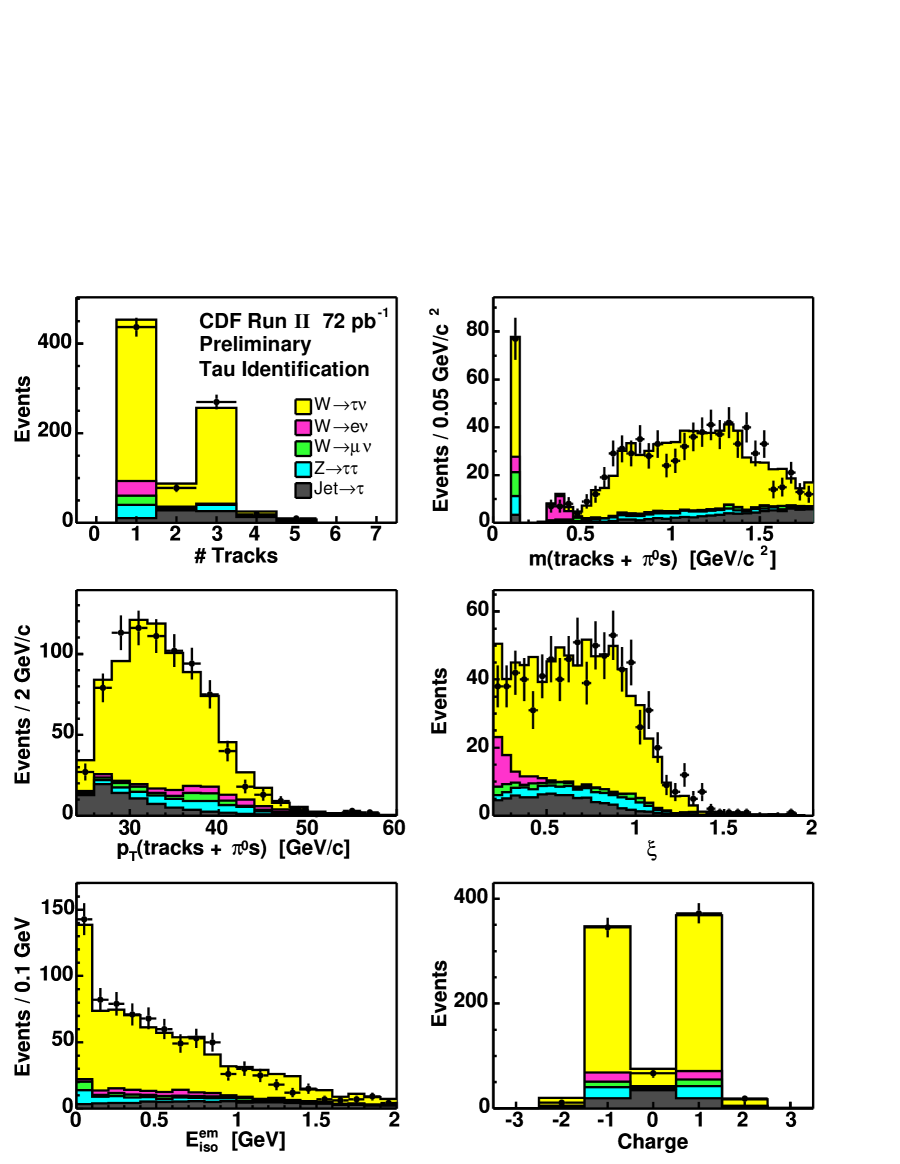
Figure 5.19: Distributions of hadronic tau identification using $W\to\tau\nu$ events for data (points) and predicted backgrounds (histograms).

5.4 Electron Identification

Identification of electrons is based on the energy it deposits in the calorimeter, its track in the COT, and its position in the CES. The central electron reconstruction algorithm [28] starts with clusters in the CEM detector. The electromagnetic towers are ordered in $E_{T}$ and the highest $E_{T}$ tower that has not yet been clustered is taken as a seed. The available shoulder towers are added to the cluster if they are adjacent in $\eta$ to the seed, and the clusters are restricted to two towers. The default threshods for seed towers and shoulder towers are 3.0 and 0.1 GeV, respectively. For the leading electrons used in our analysis with $e+\tau_{h}$ channel, the threshods for seed towers and shoulder towers are set to be 8 and 7.5 GeV, respectively. Then we associate tracks with the candidate cluster. For all of the tracks associated, the one with highest $p_{T}$ is chosen as the matched one. The CES strip and wire clusters are associated with the CEM cluster if they are reconstructed in the same wedge. The “best-matching” CES cluster is the one seeded by the matched track.

5.4.1 Electron Identification Cuts

The electron identification [29] cuts, and the conversion veto [30] cuts to remove electrons from photon conversion, are listed in Table 5.6. The $E_{T}$ and $p_{T}$ thresholds are not listed because they depend on the process and trigger sample. The probe electron must be a fiducial CEM electron and pass the vertex $z$ cut.

Variable	Cut	Note	Denominator
region	==0	CEM
fiducial	==1	fiducial $X_{CES}$, $Z_{CES}$
$|z_{0}|$	$<$60 cm	vertex $z$	Probe
track ax. seg.	$\geq$3$\times$7	COT axial segments
track st. seg.	$\geq$3$\times$7	COT stereo segments
cal. isolation	$<$0.1	cone 0.4
$E_{had}/E_{em}$	$<$0.055+0.00045$\times$$E$	had./em.
$E/p$	$<$4 (for $E_{T}<$100 GeV)	cal./track with brem.
$L_{shr}$	$<$0.2	lateral shower profile
$|\Delta X|$	$<$3 cm	$X_{track}-X_{CES}$
$|\Delta Z|$	$<$5 cm	$Z_{track}-Z_{CES}$
conversion veto	$|\Delta XY|$$<$0.2 cm, and	separation, and
	$|\Delta\cot\theta|$$<$0.04	parallel	Numerator

Table 5.6: Electron identification cuts.

5.4.2 Electron Scale Factor

The electron identification scale factor is the ratio of the efficiency in data/MC. The data sample is from the TAU_ELE trigger which requires an electron with $E_{T}>$ 8 GeV, $p_{T}>$ 8 GeV/$c$ and an isolated track with $p_{T}>$ 5 GeV/$c$. We study the electron scale factor versus $E_{T}$.

• For medium-$E_{T}$ (between 5 GeV and 20 GeV) electrons, the MC uses electrons from $Z\to\tau\tau\to eX$, and in the real data we use the second leg after selecting $\Upsilon\to ee$. We require the probe electrons have $E_{T}>$ 5 GeV and $p_{T}>$ 5 GeV/$c$ in both the real data and the MC.

• For high-$E_{T}$ (above 20 GeV) electron, the MC uses electrons from $Z\to ee$, and in the real data we use the second leg after selecting $Z\to ee$. We require the probe electrons have $E_{T}>$ 20 GeV and $p_{T}>$ 10 GeV/$c$ in both the real data and the MC.

The procedure to select $\Upsilon\to ee$ events is:

• Require a tight electron with $E_{T}>$ 8 GeV, $p_{T}>$ 8 GeV/$c$ which are the trigger requirements and the electron identification cuts.

• Require a probe electron with $E_{T}>$ 5 GeV, $p_{T}>$ 5 GeV/$c$.

• Same-sign pair will be used later for fitting the slope of background and opposite-sign pair will be used later for fitting signal + background.

• Require the invariance mass of the $ee$ pair to lie in the range (0, 20) GeV/$c^{2}$.

The procedure to select $Z\to ee$ events is:

• Require a tight electron with $E_{T}>$ 20 GeV, $p_{T}>$ 10 GeV/$c$ and the electron identification cuts.

• Require a probe electron with $E_{T}>$ 20 GeV, $p_{T}>$ 10 GeV/$c$.

• Require opposite sign.

• Require the invariance mass of the $ee$ pair to lie in the range (75, 105) GeV/$c^{2}$.

The procedure to select the second leg is:

• Require exactly one $\Upsilon$ or Z boson.

• If there is one tight electron, the probe electron is the second leg.

• If there are two tight electrons, both are used as second leg.

Then we apply the set of electron identification cuts under study on the second leg electrons in data, and on the probe electrons in the MC. The result of the procedure is shown in Table 5.7.

	data			MC
	$\Upsilon\to ee$	$Z\to ee$		$Z\to\tau_{e}\tau_{x}$	$Z\to ee$
event	11922805		event	492000	398665
good run	9103020
triggered	5575584
unique	5310963
process	10373	4534	electron	175515	797330
second leg	10770	7973	match	36733	204680	Probe
track ax. seg. $\geq 3\times 7$	10687	7946	same	36665	204266
track st. seg. $\geq 3\times 7$	10165	7721	same	36448	202907
cal. isolation $<0.1$	2797	7484	same	32094	197065
$E_{had}/E_{em}<0.055$+0.00045$E$	2553	7427	same	31290	194746
$E/p<4$ (for $E_{T}<100$ GeV)	2551	7379	same	31187	194133
$L_{shr}<0.2$	2331	7318	same	30240	188653
$|\Delta X|<3$ cm	2304	7198	same	30028	186360
$|\Delta Z|<5$ cm	2292	7189	same	29976	186222
conversion veto	2249	6878	same	29714	181449	Id

Table 5.7: Number of events for electron identification efficiency measurement.

For the $Z\to ee$ selection in the real data, the backgrounds in the sample with a tight electron plus a probe electron and in the sample with two tight electrons are both negligible which is confirmed by the negligible number of same-sign events in these two samples.

For the $\Upsilon\to ee$ in the real data, the backgrounds in the sample with tight electron plus probe electron and in the sample with two tight electrons are both significant. The same-sign samples provide the shapes of the invariant mass distribution of the backgrounds, which are taken as the slopes of linear backgrounds. Then in the opposite sign samples we fit the invariant mass distributions by the “Crystal Ball” function [31] plus a linear background. The $\Upsilon\to ee$ invariant mass distribution has a Bremsstrahlung tail at lower mass side where at least one of the electrons radiates. The “Crystal Ball” line-shape serves to model this Gaussian core with a power-law tail. The yield of signal is obtained by the entries in the histogram subtracted by the integral of the linear background.

Up to this point, all of the $\Upsilon\to ee$ candidates in the mass window (0, 20) GeV/$c^{2}$ are accepted. We then subtract background, as shown in Fig. 5.21. The plot only shows the mass window (4, 15.5) GeV/$c^{2}$. The fit is performed in the mass window (5, 12.2) GeV/$c^{2}$. The fitting result is N(e + probe) = 818.0, N(e + Id) = 644.4, efficiency = 78.8%.

Now we put everything together to get the electron scale factor vs. $E_{T}$ and perform a fit in $E_{T}$. This is shown in Fig. 5.21. Data: the medium $E_{T}$ electrons (5, 20) GeV are from the second leg of $\Upsilon\to ee$; the high $E_{T}$ electrons (30, 100) GeV are from the second leg of $Z\to ee$; there is a gap (20, 30) GeV which has very low statistics and is not used. MC: the medium $E_{T}$ electrons (5, 20) GeV are from the probe electrons of $Z\to\tau\tau\to eX$; the high $E_{T}$ electrons (30, 100) GeV are from the probe electrons of $Z\to ee$. In each $E_{T}$ bin, the efficiency in data divided by the efficiency in MC gives scale factor in that $E_{T}$ bin. For all of the $E_{T}$ bins, the scale factor is flat. A fit by a polynomial of degree 0, which is exactly the same as the weighted average, gives a scale factor $0.974\pm 0.004$.

There are two bins (45, 50) GeV and (50, 100) GeV with efficiency close to 100%, in data and MC. The binomial uncertainty in this case is always close to zero and underestimated. This propagates to the scale factors in those two $E_{T}$ bins, and finally propagates to the weighted average. There is also uncertainty in the (5, 20) GeV bin due to $\Upsilon\to ee$ background subtraction. This uncertainty is not estimated. We assign a conservative 4% uncertainty for electron scale factor [32]:

$$f^{e}_{data/MC}=0.97\pm 0.04$$ (5.23)

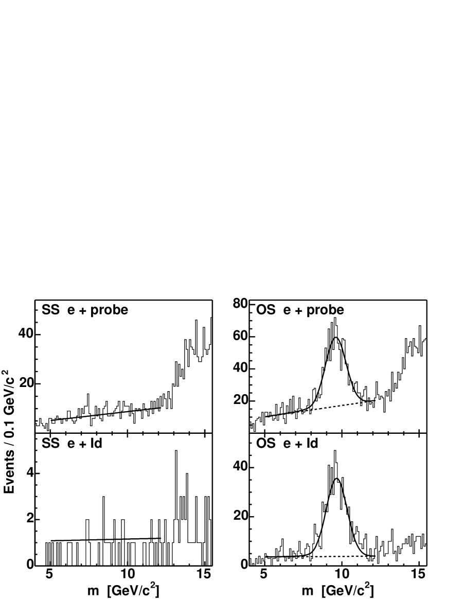
Figure 5.20: Distributions of the invariant mass of $\Upsilon\to ee$ for medium $E_{T}$ electron identification efficiency measurement in data. Same-sign samples provide the slopes of the linear backgrounds. The numbers of $\Upsilon\to ee$ signal events are obtained from fitting the histograms with the “Crystal Ball” function plus a linear background in the oppisite-sign samples.

Figure 5.21: Electron scale factor vs. $E_{T}$. This is obtained from dividing the efficiency in data by the efficiency in MC.

5.5 Muon Identification

Muon reconstruction [33] uses information from tracking, the calorimeters and the muon chambers. The momentum is measured by the curvature of the muon trajectory bent by magnetic field in tracking system. Muons behave as minimum ionizing particles and they are the only charged particle that can travel through the large amount of material in calorimeter with a very small energy loss. Muons are not stable, but they are so long lived that they can reach the muon chamber, leave hits there, and continue to travel and decay outside the detector. These features allow a rather simple and clean muon identification.

5.5.1 Muon Identification Cuts

The muon identification cuts [34] are listed in Table 5.8. We use COT-only tracks and add the beam constraint to the track. The $E_{T}$ and $p_{T}$ thresholds are not listed because they depend on the process and trigger. For data/MC scale factor studies, we require the track to be fiducial which means that the track is headed in a direction that will lead it to hit enough chambers for a stub to be reconstructed. All three subdetectors CMU, CMP, and CMX which are used in this analysis require 3 hits in 3 different layers for a stub to be reconstructed. And we will study two kinds of data/MC scale factors:

• Muon identification scale factor. A fiducial stub muon and vertex $z$ cut are required for the probe muon for this study, called “Probe (Id)” in Table 5.8.

• Marginal muon reconstruction scale factor. We require a fiducial track and a stubless muon, which also has the information of energy loss in calorimeter, for the probe muon for this study, called “Probe (Rec)” in Table 5.8. It is not necessary to have hits in the muon chambers. The vertex $z$ cut, calorimeter isolation cut, EM energy cut, and hadronic energy cut are required. Then we check if this track has a muon stub. The default track $p_{T}$ threshold to make a stubless muon is 10 GeV; we lower it to 5 GeV to allow more medium $p_{T}$ stubless muons.

Variable	Cut	Note	Probe
$|z_{0}|$	$<$60 cm	vertex $z$	Probe (Id)
cal. isolation	$<$0.1	cone 0.4
$E_{em}$	$<$2+max(0,($p$$-$100)$\times$0.0115) GeV	EM energy
$E_{had}$	$<$6+max(0,($p$$-$100)$\times$0.028) GeV	had. energy	Probe (rec.)
$|d_{0}|$	$<$0.2 cm	impact parameter
track ax. seg.	$\geq$3$\times$7	COT ax. seg.
track st. seg.	$\geq$3$\times$7	COT st. seg.
$|\Delta x_{\mbox{CMU}}|$	$<$3 cm (for CMUP)	$x_{\mbox{track}}-x_{\mbox{CMU}}$
$|\Delta x_{\mbox{CMP}}|$	$<$5 cm (for CMUP)	$x_{\mbox{track}}-x_{\mbox{CMP}}$
$|\Delta x_{\mbox{CMX}}|$	$<$6 cm (for CMX)	$x_{\mbox{track}}-x_{\mbox{CMX}}$
$\rho_{\mbox{COT}}$	$>$140 cm (for CMX)	COT exit radius

Table 5.8: Muon identification cuts.

5.5.2 Muon Scale Factor

The muon identification scale factor is the ratio of the identification efficiency in real data to that in MC. The muon marginal reconstruction scale factor is the ratio of the marginal reconstruction efficiency in data/MC. The data sample is from the TAU_CMU trigger which requires a CMUP muon with $p_{T}>$ 8 GeV/$c$ and an isolated track with $p_{T}>$ 5 GeV/$c$. (A CMUP muon is required to have stubs in both CMU and CMP). We study the muon scale factors versus muon $p_{T}$.

• For medium $p_{T}$ (between 5 and 20 GeV/$c$) muons, the MC uses muon from $Z\to\tau\tau\to\mu X$, data uses the second leg after selecting $\Upsilon\to\mu\mu$. We require the probe muons have $p_{T}>$ 5 GeV/$c$ in both the real data and the MC.

• For high $p_{T}$ (above 20 GeV/$c$) muons, the MC uses muon from $Z\to\mu\mu$, and for the data we use the second leg after selecting $Z\to\mu\mu$. We require the probe muons have $p_{T}>$ 20 GeV/$c$ in both the real data and the MC.

The procedure to select $\Upsilon\to\mu\mu$ events is:

• Cosmic veto [26].

• Require a tight CMUP muon with $p_{T}>$ 8 GeV/$c$ which are trigger requirements and the CMUP muon identification cuts.

• Require a probe muon with $p_{T}>$ 5 GeV/$c$.

• Require $|z_{0}(1)-z_{0}(2)|<$ 4 cm.

• Require opposite sign.

• Mass window (7, 13) GeV/$c^{2}$. We will use side band for background subtraction.

The procedure to select $Z\to\mu\mu$ events is:

• Cosmic veto.

• Require a tight CMUP muon with $p_{T}>$ 20 GeV/$c$ and the CMUP muon identification cuts.

• Require a probe muon with $p_{T}>$ 20 GeV/$c$.

• Require $|z_{0}(1)-z_{0}(2)|<$ 4 cm.

• Require opposite sign. The negligible number of same sign events confirms that background is negligible.

• Mass window (80, 100) GeV/$c^{2}$.

The procedure to select the second leg is:

• Require exactly one $\Upsilon$ or Z boson.

• If one tight muon, the probe muon is the second leg.

• If two tight muons, both are used as second leg.

Muon Identification Scale Factor

In the muon identification scale factor study, we apply the set of muon identification cuts under study on the second leg muons in data, and on the probe muons in the MC. Table 5.9 shows the procedure in data and Table 5.10 shows the procedure in MC.

	$\Upsilon\to\mu\mu$		$Z\to\mu\mu$
event	11922805
good run	9103020
triggered	1881529
unique	1800059
process	971		2025
second leg	1047		2805
	CMUP	CMX	CMUP	CMX
	762	285	1820	985	Probe
$|d_{0}|<0.2$ cm	758	283	1816	982
track ax. seg. $\geq 3$$\times$7	756	283	1814	978
track st. seg. $\geq 3$$\times$7	739	280	1777	955
cal. isolation $<0.1$	527	194	1750	947
$E_{em}<$ 2+max(0,($p$$-$100)$\times$0.0115) GeV	525	191	1700	929
$E_{had}<$ 6+max(0,($p$$-$100)$\times$0.028) GeV	524	191	1670	907
$|\Delta x_{\mbox{CMU}}|<3$ cm ($|\Delta x_{\mbox{CMX}}|<5$ cm)	427	129	1590	877
$|\Delta x_{\mbox{CMP}}|<6$ cm ($\rho_{\mbox{COT}}>140$ cm)	287	113	1560	753	Id

Table 5.9: Number of events for muon identification efficiency measurement in data.

	$Z\to\tau_{\mu}\tau_{x}$		$Z\to\mu\mu$
event	492000		405291
muon	170596		810582
match	32388		170382
	CMUP	CMX	CMUP	CMX
	20516	11872	107481	62901	Probe
$|d_{0}|<0.2$ cm	20499	11827	107410	62692
track ax. seg. $\geq 3$$\times$7	20490	11732	107348	62184
track st. seg. $\geq 3$$\times$7	20417	11601	106985	61463
cal. isolation $<0.1$	18361	10448	104247	59929
$E_{em}<$ 2+max(0,($p$$-$100)$\times$0.0115) GeV	18055	10261	100115	57680
$E_{had}<$ 6+max(0,($p$$-$100)$\times$0.028) GeV	17871	10080	97906	55799
$|\Delta x_{\mbox{CMU}}|<3$ cm ($|\Delta x_{\mbox{CMX}}|<5$ cm)	16799	8994	97707	55617
$|\Delta x_{\mbox{CMP}}|<6$ cm ($\rho_{\mbox{COT}}>140$ cm)	14198	7419	96788	46059	Id

Table 5.10: Number of events for muon identification efficiency measurement in MC.

Up to this point, all of the $\Upsilon\to\mu\mu$ candidates in mass window (7, 13) GeV/$c^{2}$ are accepted. Now we break the probe into two $p_{T}$ bins 5 $<p_{T}<$ 10 GeV/$c$ and 10 $<p_{T}<$ 20 GeV/$c$. Fig. 5.23 shows the distributions of the pair mass of the first leg and the second leg in each $p_{T}$ bin of the second leg, for CMUP probe. We see three clear peaks at about 9.5, 10 and 10.3 GeV/$c^{2}$. This is the signature of $\Upsilon\to\mu\mu$. Now we subtract the linear background. The signal mass window is defined as (9.2, 10.6) GeV/$c^{2}$. We use a side-band method: yield = entries in (9.2, 10.6) $-$ entries in (7.8, 8.5) $-$ entries in (11.3, 12) GeV/$c^{2}$ mass windows. In $5<p_{T}<10$ ($10<p_{T}<20$) GeV/$c$ bin, N(muon + probe) = 410 (85), N(muon + Id) = 168 (56), we get efficiency = 41.0% (65.9%). We put everything together to get the CMUP muon identification scale factor vs. $p_{T}$ and perfom a fit in $p_{T}$. This is shown in Fig. 5.23.

Fig. 5.25 shows the mass distribution of muon pair in each $p_{T}$ bin of the second leg, for CMX probe. In $5<p_{T}<10$ ($10<p_{T}<20$) GeV/$c$ bin, N(muon + probe) = 126 (32), N(muon + Id) = 57 (19), we get efficiency = 45.2% (59.4%). Fig. 5.25 shows the procedure to get the CMX muon identification scale factor.

Analogous to the electron scale factor study, we assign a conservative uncertainty of 4%. The resulting identification scale factors are $0.93\pm 0.04$ for CMUP muon, and $1.03\pm 0.04$ for CMX muon.

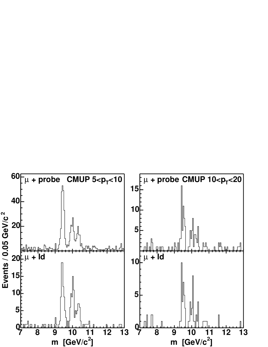
Figure 5.22: Distributions of the invariant mass of $\Upsilon\to\mu\mu$ for medium $p_{T}$ CMUP muon identification efficiency measurement in data. The three peaks are signature of $\Upsilon\to\mu\mu$. The left two plots are for CMUP muons with $5<p_{T}<10$ GeV/$c$. The right two plots are for CMUP muons with $10<p_{T}<20$ GeV/$c$. Side-band method is used for background subtractions.

Figure 5.23: CMUP muon identification scale factor vs. $p_{T}$. This is obtained from dividing the efficiency in data by the efficiency in MC.

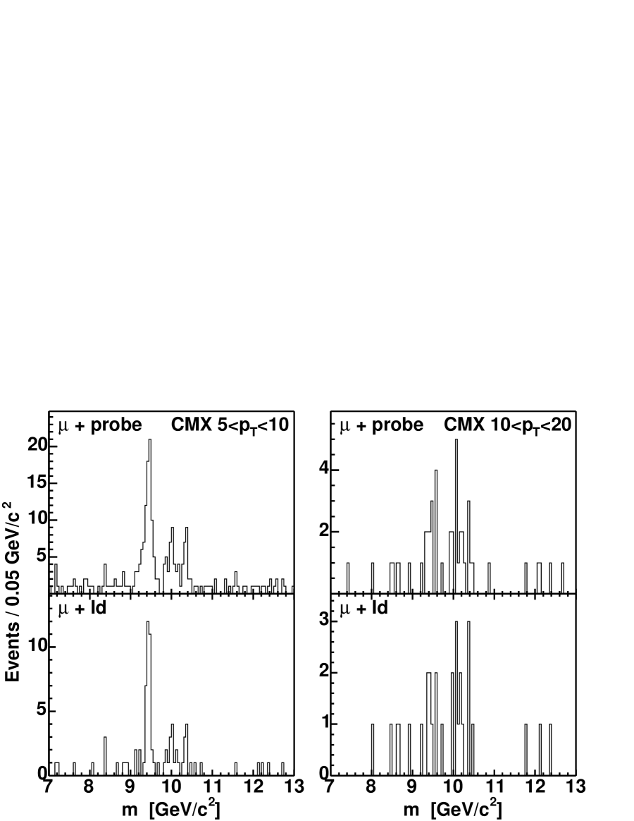
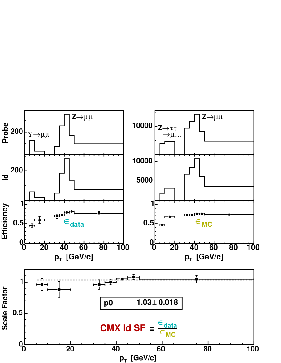
Figure 5.24: Distributions of the invariant mass of $\Upsilon\to\mu\mu$ for medium $p_{T}$ CMX muon identification efficiency measurement in data. The three peaks are signature of $\Upsilon\to\mu\mu$. The left two plots are for CMX muons with $5<p_{T}<10$ GeV/$c$. The right two plots are for CMX muons with $10<p_{T}<20$ GeV/$c$. Side-band method is used for background subtractions.

Figure 5.25: CMX muon identification scale factor vs. $p_{T}$. This is obtained from dividing the efficiency in data by the efficiency in MC.

Muon Reconstruction Scale Factor

In the reconstruction scale factor study, the probe is a stubless muon which may or may not have a stub in the muon chamber associated with the fiducial track. It must have passed the vertex $z$ cut, calorimeter isolation, EM energy cut, and hadronic energy cut. For such a probe, we check if it has a stub. Table 5.11 shows the procedure in data and Table 5.12 shows the procedure in MC.

	$\Upsilon\to\mu\mu$		$Z\to\mu\mu$
event	11922805
goodrun	9103020
triggered	1881529
unique	1800059
process	691		1861
second leg	760		2583
	CMUP	CMX	CMUP	CMX
	570	190	1718	865	Probe
has stub	474	170	1569	838	Rec.

Table 5.11: Number of events for muon reconstruction efficiency measurement in data.

	$Z\to\tau_{\mu}\tau_{x}$		$Z\to\mu\mu$
event	492000		405291
muon	170596		810582
match	27109		149411
	CMUP	CMX	CMUP	CMX
	17334	9775	95503	53908	Probe
has stub	16672	9709	93044	53827	Rec.

Table 5.12: Number of events for muon reconstruction efficiency measurement in MC.

We break the second leg muon into two $p_{T}$ bins: 5 $<p_{T}<$ 10 GeV/$c$ and 10 $<p_{T}<$ 20 GeV/$c$. Fig. 5.27 shows the distributions of the pair mass of the first leg and the second leg in each $p_{T}$ bin of the second leg, for CMUP probe. We use the side-band method to do background subtraction. In $5<p_{T}<10$ ($10<p_{T}<20$) GeV/$c$ bin, N(muon + probe) = 307 (65), N(muon + stub) = 272 (59), we get efficiency = 88.6% (90.8%). We put everything together to get the muon reconstruction scale factor vs. $p_{T}$ and perform a fit in $p_{T}$. This is shown in Fig. 5.27.

Fig. 5.29 shows the mass distribution of muon pair in each $p_{T}$ bin of the second leg, for CMX probe. In $5<p_{T}<10$ ($10<p_{T}<20$) GeV/$c$ bin, N(muon + probe) = 92 (22), N(muon + stub) = 85 (21), we get efficiency = 92.4% (95.5%). Fig. 5.29 shows the procedure to get the CMX muon reconstruction scale factor.

As in the electron scale factor study, we assign a conservative systematic uncertainty of 4%. The results of the reconstruction scale factors are $0.94\pm 0.04$ for CMUP muon, and $0.97\pm 0.04$ for CMX muon.

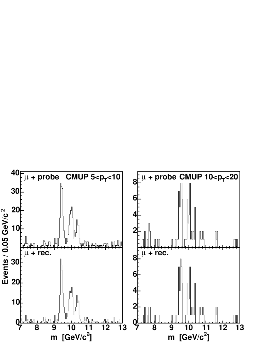
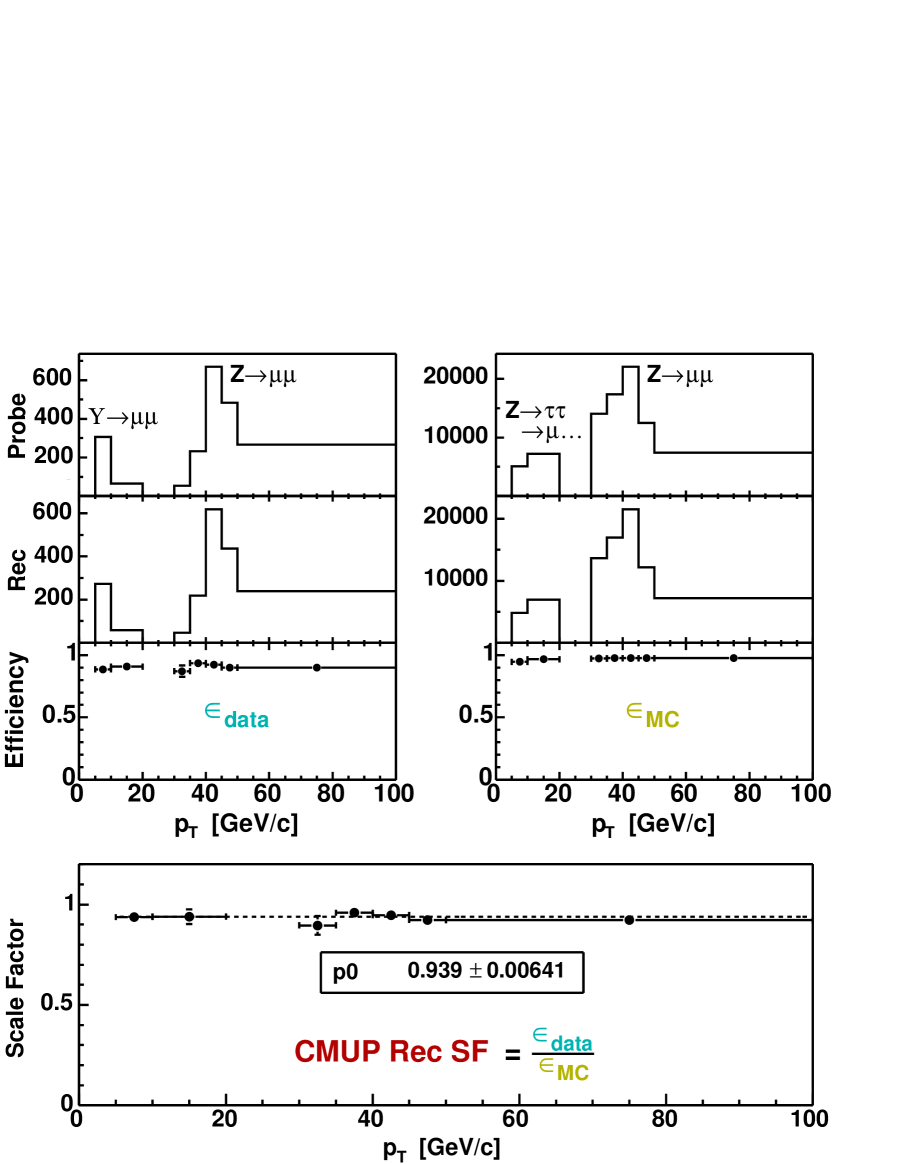
Figure 5.26: Distributions of the invariant mass of $\Upsilon\to\mu\mu$ for medium $p_{T}$ CMUP muon reconstruction efficiency measurement in data. The three peaks are signature of $\Upsilon\to\mu\mu$. The left two plots are for CMUP muons with $5<p_{T}<10$ GeV/$c$. The right two plots are for CMUP muons with $10<p_{T}<20$ GeV/$c$. Side-band method is used for background subtractions.

Figure 5.27: CMUP muon reconstruction scale factor vs. $p_{T}$. This is obtained from dividing the efficiency in data by the efficiency in MC.

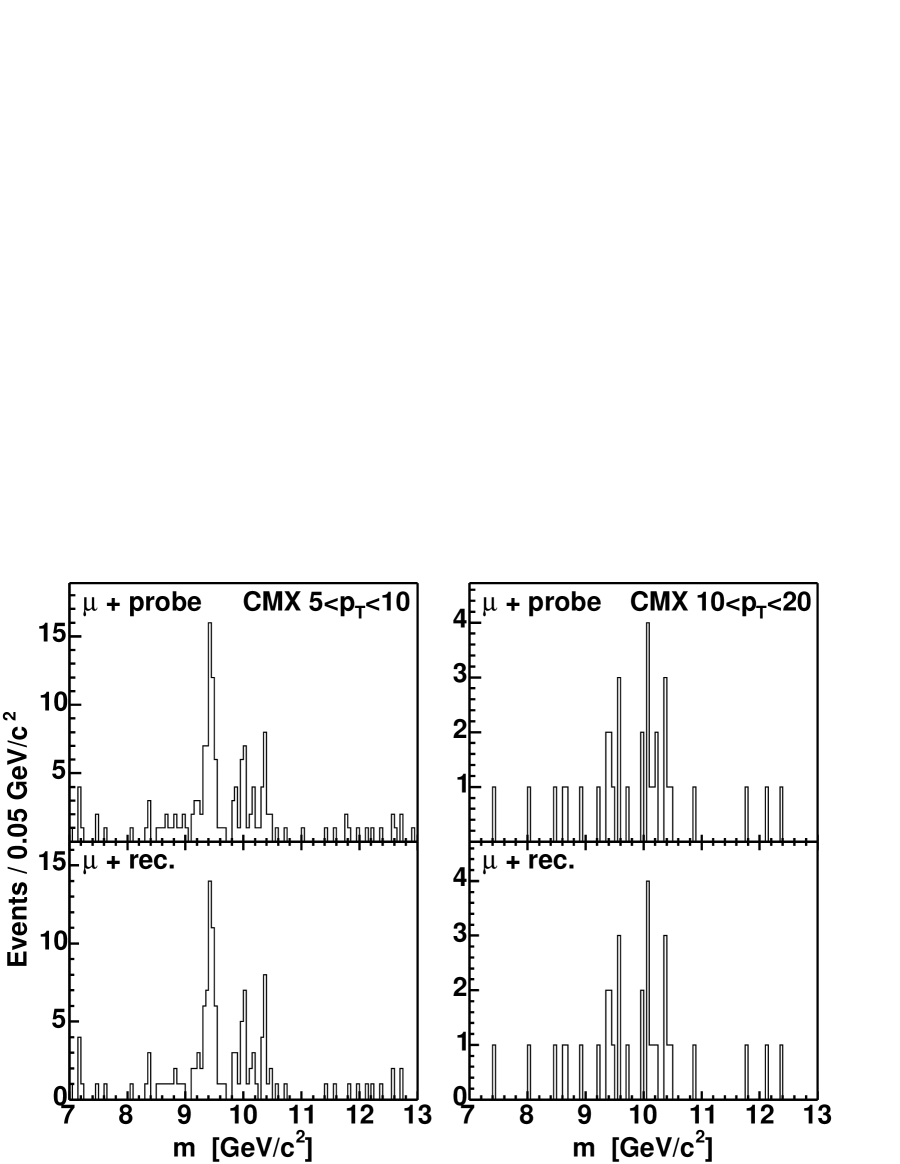
Figure 5.28: Distributions of the invariant mass of $\Upsilon\to\mu\mu$ for medium $p_{T}$ CMX muon reconstruction efficiency measurement in data. The three peaks are signature of $\Upsilon\to\mu\mu$. The left two plots are for CMX muons with $5<p_{T}<10$ GeV/$c$. The right two plots are for CMX muons with $10<p_{T}<20$ GeV/$c$. Side-band method is used for background subtractions.

Figure 5.29: CMX muon reconstruction scale factor vs. $p_{T}$. This is obtained from dividing the efficiency in data by the efficiency in MC.

We summarize the muon reconstruction and identification scale factors with uncertainties:

$$f^{CMUP\;\;rec}_{data/MC} = 0.94\pm 0.04$$ (5.24)

$$f^{CMUP\;\;Id}_{data/MC} = 0.93\pm 0.04$$ (5.25)

$$f^{CMX\;\;rec}_{data/MC} = 0.97\pm 0.04$$ (5.26)

$$f^{CMX\;\;Id}_{data/MC} = 1.03\pm 0.04$$ (5.27)

5.6 Missing Transverse Energy

Weakly interacting particles such as neutrinos of the Standard Model and the lightest supersymmetric particle (LSP) predicted in new physics, deposit no energy in the calorimeters. Minimum ionizing particles such as muons leave little energy in the calorimeters. When present these cause a significant vector sum of the transverse energy of all of the detected particles. The imbalance, i.e., the negative of the vector sum in the transverse plane corresponds to the missing transverse energy ($\,/\!\!\!\!E_{T}$).

Since $\,/\!\!\!\!E_{T}$ measures the vector sum of all of the momentum of particles escaping detection in the calorimeters, there is no information on the energy and direction of an individual particle or how many particles escaped detection. With many such particles in an event there is also a chance that their transverse momenta cancel each other.

There is an instrumental source of $\,/\!\!\!\!E_{T}$ because the calorimeters are not perfect. There are crack regions due to the support structures, and the transition regions between components, for example from the central calorimeters to the plug calorimeters. The probability that all the energy of a particle is undetected is rather small. But QCD processes have a large production rate. Some of the jets can have a lot of energy undetected and make a significant $\,/\!\!\!\!E_{T}$.

In our high-mass tau pair analysis, we will use an $\,/\!\!\!\!E_{T}$ cut and several other kinematic cuts related to $\,/\!\!\!\!E_{T}$. To get the uncertainty due to the instrumental $\,/\!\!\!\!E_{T}$, we should get the distributions in data and MC, and compare the same variable.

In the real data, the physics processes $Z\to ee$ and $\gamma$ + jet, which have zero true missing energy, can be used to study the effect of the instrumental $\,/\!\!\!\!E_{T}$. The latter is a better choice for our purpose because hadronic taus in the calorimeters are more like jets than electrons. The inclusive photon sample is used to select $\gamma$ + jet events. Jets are required to be reconstructed as hadronic tau objects. The true $\,/\!\!\!\!E_{T}$ in this sample should be zero. The reconstructed $\,/\!\!\!\!E_{T}$ corresponds to the instrumental $\,/\!\!\!\!E_{T}$ in data.

The simulation uses $Z\to\tau_{e}\tau_{h}$ process and requires a tight electron and a hadronic tau object. The difference between the reconstructed $\,/\!\!\!\!E_{T}$ in the simulation minus the $\,/\!\!\!\!E_{T}$ from neutrinos corresponds to the instrumental $\,/\!\!\!\!E_{T}$ in MC.

Then the instrumental $\,/\!\!\!\!E_{T}$ is projected to the direction of hadronic tau object, shown in Fig. 5.30. The distributions in data and MC are different for the longitudinal component and the transverse component, respectively.

To get the uncertainty due to the instrumental $\,/\!\!\!\!E_{T}$, we “smear” the longitudinal component and the transverse component of the instrumental $\,/\!\!\!\!E_{T}$ in MC according to their differences between data and MC, then add neutrinos back to get the smeared $\,/\!\!\!\!E_{T}$.

Now we can calculate the uncertainty of the cuts related to $\,/\!\!\!\!E_{T}$ by the effect with/without smearing the instrumental $\,/\!\!\!\!E_{T}$. Table 5.13 shows the effect in $\tau_{e}\tau_{h}$ channel of $Z^{\prime}(m=300\mbox{ GeV/}c^{2})$ sample and $Z^{\prime}(m=600\mbox{ GeV/}c^{2})$ sample. The uncertainties are (1191-1125)/1125 = 5.9% in $Z^{\prime}(300)$ sample and (1875-1814)/1814 = 3.4% in $Z^{\prime}(600)$ sample. Taking the larger value, we find that the uncertainty in acceptance due to $\,/\!\!\!\!E_{T}\approx 6\%$.

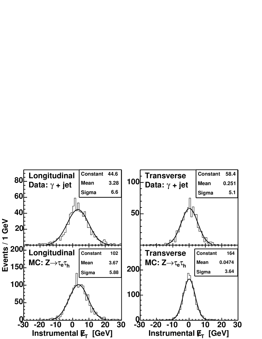
Figure 5.30: Distributions of the instrumental $\,/\!\!\!\!E_{T}$ in data using $\gamma$+jet sample and MC using $Z\to\tau_{e}\tau_{h}$ sample. Instrumental $\,/\!\!\!\!E_{T}$ is projected to the direction of the reconstructed leading tau object to get the longitudinal and transverse components.

sample	$Z^{\prime}(m=300\mbox{ GeV/}c^{2})$		$Z^{\prime}(m=600\mbox{ GeV/}c^{2})$
$\tau\tau$ event	100000		100000
$\tau_{e}\tau_{h}$ decay mode	23246		23250
$E_{T}^{e}>$ 10 GeV, $p_{T}^{\tau}>25$ GeV/$c$	2135		3044
smear instrumental $\,/\!\!\!\!E_{T}$	no	yes	no	yes
$\,/\!\!\!\!E_{T}>$ 15 GeV	1720	1801	2745	2829
$\Delta\phi(e-\,/\!\!\!\!E_{T})<30^{\circ}$	1231	1299	1844	1907
$m_{vis}>$ 120 GeV/$c^{2}$	1125	1191	1814	1875
uncertainty	5.9%		3.4%

Table 5.13: Number of $Z^{\prime}\to\tau\tau$ events to study the uncertainty in acceptance due to the imperfect modeling of the instrumental $\,/\!\!\!\!E_{T}$ in MC simulation. The uncertainty is obtained from the effect of with/without “smearing” the instrumental $\,/\!\!\!\!E_{T}$ in MC to that in data.

Chapter 6 Event Kinematic Selection

In this chapter we first discuss the trigger paths. Second, we discuss the good run selections and the integrated luminosities. Third, in addition to the particle identification, we add event kinematic cuts to further suppress backgrounds. Since the kinematic cuts need to keep high efficiency for the signals, optimization on the event kinematic cuts is necessary. Fourth, there are thresholds in the triggers. The trigger primitives are not exactly the same as the offline variables we cut on, and so we need to evaluate the marginal trigger efficiencies for selected events.

6.1 Trigger Path

For the $\tau_{e}\tau_{h}$ selection, we use the “electron plus track” trigger called TAU_ELE. It requires an electron in the CEM detector with $E_{T}>8$ GeV, $p_{T}>8$ GeV/$c$ and an isolated track with $p_{T}>5$ GeV/$c$.

For the $\tau_{\mu}\tau_{h}$ selection, there are two “muon plus track” triggers called TAU_CMU (TAU_CMX) which requires a CMUP (CMX) muon with $p_{T}>8$ GeV/$c$ and an isolated track with $p_{T}>5$ GeV/$c$.

For the $\tau_{h}\tau_{h}$ selection, we use the “$\,/\!\!\!\!E_{T}$ plus tau” trigger called TAU_MET. It requires L1 $\,/\!\!\!\!E_{T}>25$ GeV and an L3 tau object with $E_{T}>20$ GeV, track isolation and $m$(tracks) $<2.0$ GeV/$c^{2}$.

The TAU_ELE, TAU_CMU, and TAU_CMX triggers are cleaned up by requiring an isolated track. The TAU_MET trigger requires only one isolated tau object thus the other tau objects in this trigger are not necessarily isolated.

The track isolation requirement in these triggers is that there is no additional track in a 10^o to 30^o annulus. This track isolation is looser than the offline tau track isolation with a shrinking inner cone. The detailed descriptions of the tau triggers can be found in Ref. [35].

In addition to selecting the candidate events, there is also an important issue regarding the jet$\to\tau$ misidentification background. This fake background is not negligible because of the large production rate of jets. Using MC simulation to model all the processes of the fake background is not adequate. We estimate the contribution of these events directly from real data.

For the purpose of estimating jet$\to\tau$ misidentification background, it is better to use those triggers without the isolation requirement in order to have a sample which has a larger statistics and is dominated by jet background.

There is an ELECTRON_CENTRAL_8 (abbreviated as CELE8) trigger which has the same requirement as TAU_ELE but without the track isolation requirement. There is also a MUON_CMUP8 (abbreviated as CMUP8) trigger which has the same requirement as TAU_CMU but without the track isolation requirement. The CELE8 and the CMUP8 triggers are dynamically prescaled. A prescale is imposed to reduce the rate of a trigger. A fixed prescale under-utilizes the trigger bandwidth when the luminosity falls during a run. A dynamic prescale is based on the availability of the trigger bandwidth, and automatically reduce the prescales as the luminosity falls.

There is not a corresponding trigger path available for the TAU_CMX trigger. There is a prescaled trigger available for the TAU_MET trigger but its prescale is 100 which is too big. Thus their jet$\to\tau$ fake background estimates have to be done with the trigger itself.

6.2 Good Run Selection and Integrated Luminosity

We use the data samples collected in CDF from March 2002 to September 2003 for this analysis. The Good Run List [36] used in this analysis is in the range of the run number 141544$-$168889.

We use the online initial filtering and the offline periodic classification to decide whether a run is good or bad. The former gets rid of obviously bad runs where there are problems with the sub-detectors or the triggers. The latter is based on the classification using a large sample in a run, for example, of the $J/\Psi\to ee,\;\mu\mu$ events which is expected to have a very narrow peak, or the photon plus jet events which is expected to have very good energy balancing, etc.

The status of a trigger or a sub-detector is a single bit 1 or 0, which means good or bad. The bit 1 or 0 of a trigger is based on whether the deadtime is less than 5% and is set by the online run control shift crew. The bit 1 or 0 of a sub-detector at the online stage is based on the status of the high voltage, the calibration, the occupancy, etc. and is set by the monitoring operator. The bit 1 or 0 of a sub-detector at the offline stage is based on, for example, the reconctructed $J/\Psi\to ee,\;\mu\mu$ mass which can tell possible problems in the tracking system, the calorimeters or the muon chambers, and is set by the physics groups.

Here are the details of the requirements on a good run. There are several run configurations (trigger tables) when the CDF detector is taking data: test, calibration, cosmic, and physics. A good run must be a physics run. At the online stage the losses of the beam should be low. The “on-tape” luminosity should be greater than 10 nb^-1. The bits of the L1, L2, L3 triggers, the calorimeters, the CMU detector, the CES detector should be 1. At the offline stage the bits of the calorimeters, the COT detector, the CMU and CMP detectors should be 1. The runs after 150145 when the CMX trigger updated L1 hardware, in addition to the bits above, are required to have the online and offline bits of the CMX detector set to 1.

The total integrated luminosity in the included good runs in the run number range 141544$-$168889 is 195 pb^-1. However, the good run of the data sample from the TAU_CMX trigger starts from 150145 and its integrated luminosity is 179 pb^-1; the good run number of the data sample from the TAU_MET trigger stops at 156487 and its integrated luminosity is 72 pb^-1. The TAU_MET trigger was changed after run 156487 to include L2 two-dimensional track isolation which needs further study. The uncertainty in the luminosity measurements is about 6% [27].

The integrated luminosity in the data sample from the CELE8 trigger, which is dynamically prescaled, is 46 pb^-1. It is calculated by adding the isolated track requirement and comparing its survived number of events with the total number of events in the data sample from the TAU_ELE trigger whose luminosity is known. Analogously, the integrated luminosity in the data sample from the CMUP8 trigger is found to be 38 pb^-1.

There were duplicate events incorrectly processed and put in the data samples that were later reprocessed. We reprocessed all of the events. To avoid the duplicate events, we pick one of them and require that it be a unique event.

6.3 Selection Criteria

The event kinematic cuts are designed to further suppress background while to keep high signal efficiency. Table 6.1 shows the list of cuts for event selection. We note several features of the requirements:

• The $p_{T}^{\tau}$ threshold is 25 GeV/$c$ because tau identification is fully efficient at about 25 GeV/$c$ and it is a high threshold to reduce background.

• The $E_{T}^{e}$, $p_{T}^{e}$, and $p_{T}^{\mu}$ thresholds are 10 GeV, 10 GeV/$c$ and 10 GeV/$c$, respectively. (The thresholds in the corresponding triggers are 8 GeV, 8 GeV/$c$ and 8 GeV/$c$.) For $\tau_{h}\tau_{h}$, we require the second tau $p_{T}^{\tau_{2}}>10$ GeV/$c$.

• The $\,/\!\!\!\!E_{T}$ cut and the angle cut $\Delta\phi(l-\,/\!\!\!\!E_{T})<30^{o}$ are designed to remove hadronic jet backgrounds. They are explained below.

• We use $m_{vis}>$ 120 GeV/$c^{2}$ cut to remove the “irreducible” $Z/\gamma^{*}\to\tau\tau$ background. The low mass region with $m_{vis}<$ 120 GeV/$c^{2}$ is our control region.

• For the $\tau_{\mu}\tau_{h}$ selection, we have a cosmic veto [26].

• For the $\tau_{h}\tau_{h}$ selection, we require the second tau has exactly one track to further clean up QCD backgrounds. We will check tau signature by track multilicity on the leading tau side.

$\tau_{e}\tau_{h}$	$\tau_{\mu}\tau_{h}$	$\tau_{h}\tau_{h}$
$p_{T}^{\tau}>25$	$p_{T}^{\tau}>25$	$p_{T}^{\tau_{1}}>25$
$E_{T}^{e}>10$, $p_{T}^{e}>10$	$p_{T}^{\mu}>10$	$p_{T}^{\tau_{2}}>10$
$\,/\!\!\!\!E_{T}>15$	$\,/\!\!\!\!E_{T}>15$	$\,/\!\!\!\!E_{T}>25$
$\Delta\phi(e-\,/\!\!\!\!E_{T})<30^{o}$	$\Delta\phi(\mu-\,/\!\!\!\!E_{T})<30^{o}$	$\Delta\phi(\tau_{2}-\,/\!\!\!\!E_{T})<30^{o}$
$m(e+\tau+\,/\!\!\!\!E_{T})>120$	$m(\mu+\tau+\,/\!\!\!\!E_{T})>120$	$m(\tau_{1}+\tau_{2}+\,/\!\!\!\!E_{T})>120$
	cosmic veto	$\tau_{2}$ num. track == 1

Table 6.1: Event kinematic cuts.

The $\,/\!\!\!\!E_{T}$ measured in $\tau_{\mu}\tau_{h}$ channel needs a muon correction since there is an effect of missing energy due to the fact that muons are minimum ionizing partilces. The procedure of the muon correction is: first, we subtract the $p_{T}$ of a tight muon; second, we add muon energy deposits in the calorimeters to avoid counting the same energy twice.

We require $\,/\!\!\!\!E_{T}>15$ GeV for the $\tau_{e}\tau_{h}$ and $\tau_{\mu}\tau_{h}$ selections. For the $\tau_{h}\tau_{h}$ selection, we use data from the TAU_MET trigger and we require $\,/\!\!\!\!E_{T}>25$ GeV to match the 25 GeV $\,/\!\!\!\!E_{T}$ trigger threshold. We could suppress more backgrounds by requiring more significant $\,/\!\!\!\!E_{T}$. However, for the signal processes, since there is at least one neutrino at each side, there is a chance that the transverse momentum of the neutrinos cancel each other, and hence raising $\,/\!\!\!\!E_{T}$ thresholds can reduce signal efficiency. We found those $\,/\!\!\!\!E_{T}$ thresholds are at optimzed points.

The $\Delta\phi<30^{o}$ cut requires that the significant $\,/\!\!\!\!E_{T}$ should follow the $e$ ($\mu$) for the $\tau_{e}\tau_{h}$ ($\tau_{\mu}\tau_{h}$) channels and follow the lower $p_{T}$ tau object for the $\tau_{h}\tau_{h}$ channel. The $\,/\!\!\!\!E_{T}$ measured is the vector sum of the neutrinos from the decays of the two taus. Here is the example with the $\tau_{e}\tau_{h}$ channel which has one neutrino associated with $\tau_{h}$ and two neutrinos associated with $\tau_{e}$. Thus this event topology cut is able to get the most of the signals, and to strongly suppress the backgrounds, especially the jet$\to\tau$ misidentified fake backgrounds which mostly has a $\Delta\phi$ with a random topology.

6.4 Marginal Efficiency Correction

We need to include in our estimates of the signal and background rates the effect of the triggers. We are concerned, however, only with the effect of the triggers on those events passing the offline cuts: the marginal efficiency.

The TAU_MET trigger for the $\tau_{h}\tau_{h}$ analysis triggers directly on tau object, thus there is no marginal trigger efficiency from the TAU side. But there is a marginal trigger efficiency from the MET side which is based on a 1 GeV tower threshold for a fast calculation at L1 while the offline $\,/\!\!\!\!E_{T}$ is based on a 0.1 GeV tower threshold. We use the JET20 data sample and mimic the $\tau_{h}\tau_{h}$ event topology in the calorimeter by requiring one central jet with $E_{T}>25$ GeV and at least another one central jet with $E_{T}>10$ GeV. The L1 $\,/\!\!\!\!E_{T}>$ 25 GeV trigger efficiency vs. offline $\,/\!\!\!\!E_{T}$ for di-tau event is shown in Fig. 6.1. The marginal trigger efficiency of the TAU_MET trigger for the $\tau_{h}\tau_{h}$ analysis is a slow turn-on due to the large trigger tower threshold.

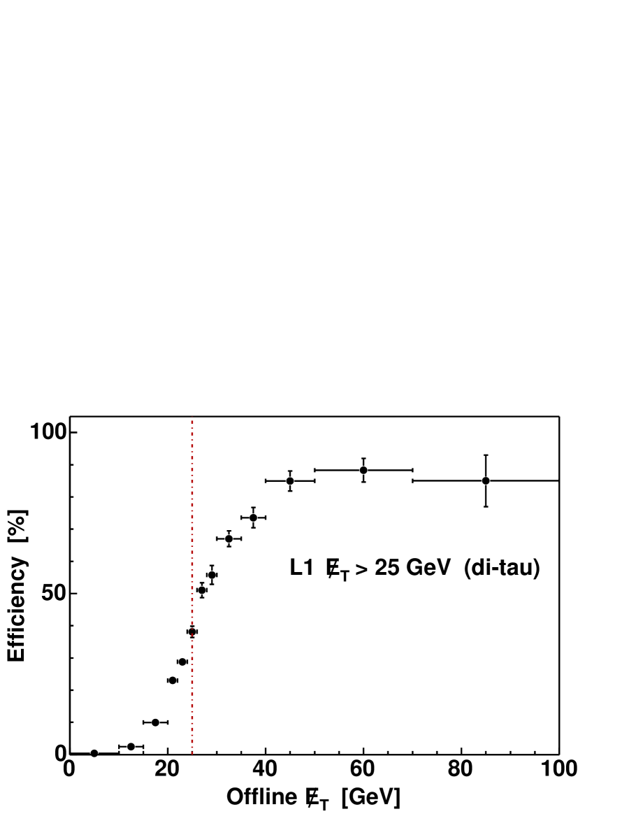
Figure 6.1: L1 $\,/\!\!\!\!E_{T}>$ 25 GeV trigger efficiency vs. offline $\,/\!\!\!\!E_{T}$ for di-tau event.

The marginal efficiencies of the TAU_ELE and TAU_CMU (TAU_CMX) triggers for the $\tau_{e}\tau_{h}$ and $\tau_{\mu}\tau_{h}$ analyses are all at plateau,

$$\epsilon\mbox{(TAU\_ELE)} = 0.92\pm 0.03$$ (6.1)

$$\epsilon\mbox{(TAU\_CMU)} = 0.85\pm 0.03$$ (6.2)

$$\epsilon\mbox{(TAU\_CMX)} = 0.92\pm 0.03$$ (6.3)

The trigger efficiencies of the electron part, the muon part and the isolated track part are calculated by using conversion electrons from $\gamma\to ee$, muons from $\Upsilon/Z\to\mu\mu$, and tracks from jet samples, respectively. The details can be found in Ref. [37]. The biggest uncertainty is from the track provided by the XFT trigger, which uses the four axial $r-\phi$ superlayers (no stereo $r-z$ superlayers) of the COT detector with at least 10 hits (out of total 12 hits) in each axial superlayer. In the event reconstruction, we require at least 3 axial superlayers with at least 7 hits in each axial superlayer, and the same configuration for the stereo superlayers. The marginal XFT track finding trigger efficiency is found to be a function of $p_{T}$, $\eta$, the number of prongs, and the different run ranges. The overall uncertainty is about 3%.

Chapter 7 Low Mass Control Region

The low-mass region with $m_{vis}<120$ GeV/$c^{2}$ is used as the control region to test the event cuts and background determination. If we find that the observed and predicted event rates agree in the control region, we can proceed to unblind the signal region.

The main source of events in the control region is from $Z/\gamma^{*}\to\tau\tau$. The other backgrounds include $Z/\gamma^{*}\to ee$, $Z/\gamma^{*}\to\mu\mu$ and jet$\to\tau$ misidentified fake background. Top background $t\bar{t}$ and di-boson backgrounds such as $WW$ and $WZ$ are negligible because their cross sections are two orders of magnitude smaller than Drell-Yan backgrounds and their event topology is the opposite of the requirement that a significant $\,/\!\!\!\!E_{T}$ follows the lepton direction. The jet$\to\tau$ misidentified fake background is not negligible because the dijet production cross section is large.

For the jet$\to\tau$ misidentified fake background, rather than trying to model all the processes that could produce fake events, we estimate the contribution of these events from real data which includes any process contributing to the fake background.

7.1 Drell-Yan Cross Section

The cross section times branching ratio of the Drell-Yan processes in the mass window $66<m<116$ GeV/$c^{2}$ at $\sqrt{s}=1.96$ TeV is about 250 pb [20]. Fig. 7.1 shows the mass spectrum and event counts in different mass regions. The $Z/\gamma^{*}\to\tau\tau$ sample has 377143 events in the mass window $66<m<116$ GeV/$c^{2}$ which corresponds to a 250 pb production cross section. The number of events in a mass window is proportional to the cross section in that mass window. For example, the number of events 492000 in the mass window $m>30$ GeV/$c^{2}$ gives a cross section $250\times 492000/377143\approx 326$ pb. By the same algebra, we get the cross sections in different mass windows:

$$\sigma\cdot B(Z/\gamma^{*}\to l^{+}l^{-})_{66-116} \approx 250\mbox{ pb}$$ (7.1)

$$\sigma\cdot B(Z/\gamma^{*}\to l^{+}l^{-})_{>30\ \ \ \,} \approx 326\mbox{ pb}$$ (7.2)

$$\sigma\cdot B(Z/\gamma^{*}\to l^{+}l^{-})_{30-100} \approx 315\mbox{ pb}$$ (7.3)

$$\sigma\cdot B(Z/\gamma^{*}\to l^{+}l^{-})_{>100\ \ \,} \approx \ \,11\mbox{ pb}$$ (7.4)

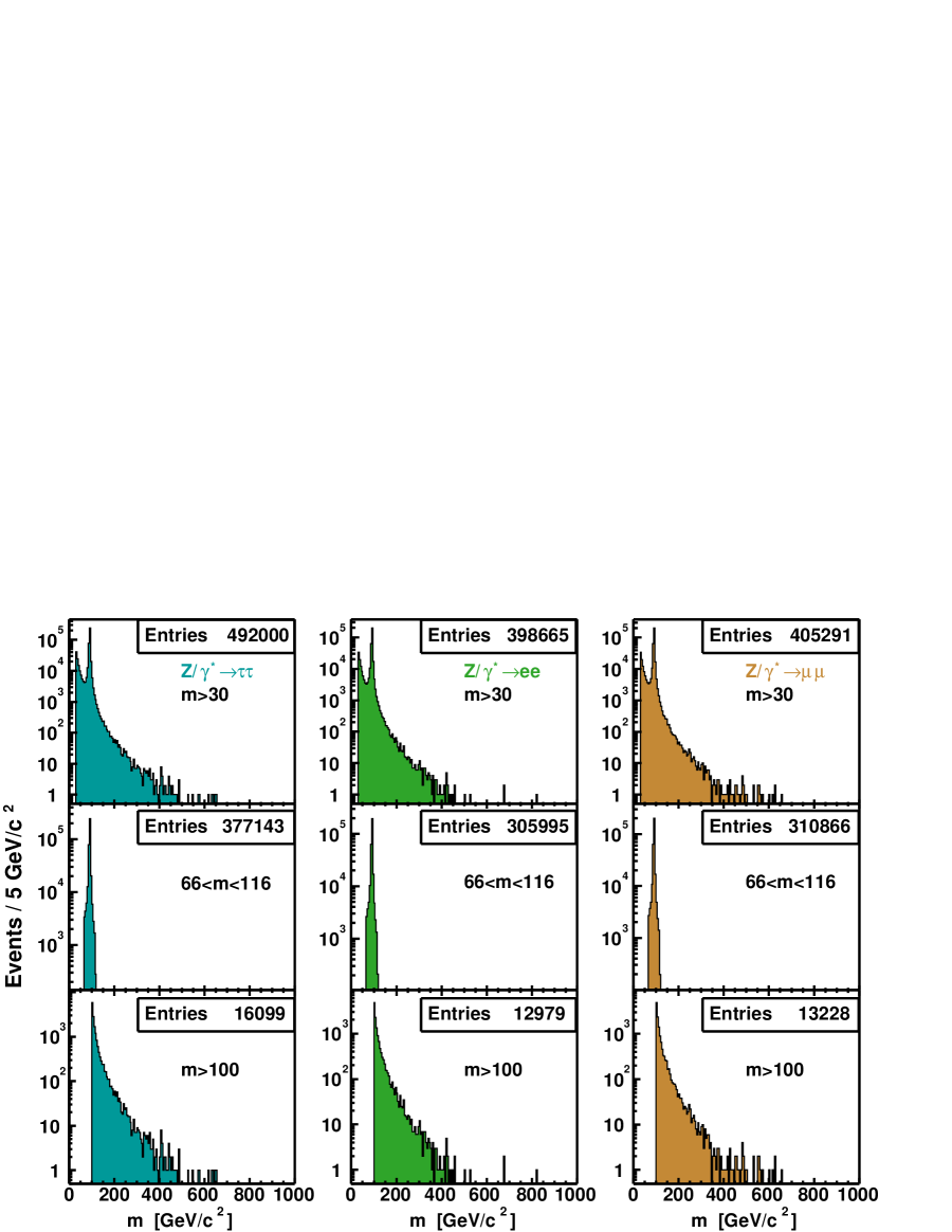
Figure 7.1: Drell-Yan mass spectra in different mass regions.

7.2 Drell-Yan Background

The Drell-Yan backgrounds can be estimated from MC simulation with three pieces:

$$\mbox{Expected MC background}=\mbox{luminosity}\times(\sigma\cdot B)\times\mbox{acceptance}$$ (7.5)

We just discussed the production cross section, and we have discussed the luminosity for each trigger path in Section 6.2. Now we discuss the acceptance and the estimate of the Drell-Yan backgrounds. Table 7.1 shows the Drell-Yan background acceptances, the application of the trigger efficiencies, the application of the lepton data/MC scale factors, and the normalization to the integrated luminosities of the data samples from the triggers.

source	$Z/\gamma^{*}\to\tau\tau$	$Z/\gamma^{*}\to ee$	$Z/\gamma^{*}\to\mu\mu$
mass window	$m>30$	$m>30$	$m>30$
$\sigma\cdot B$ (pb)	326	326	326
event	492000	398665	405291
$\tau_{e}\tau_{h}$ (TAU_ELE)
$\tau(25)+e(10)$	1528	272	1
$\,/\!\!\!\!E_{T}>15$	514	29	1
$\Delta\phi(e-\,/\!\!\!\!E_{T})<30^{\circ}$	415	2	0
$m_{vis}<120$	405	1	0
trigger efficiency	373.07	0.92	0.00
lepton scale factors	351.03	0.87	0.00
normalized (195 pb-1)	45.36	0.14	0.00
$\tau_{\mu}\tau_{h}$ (TAU_CMU)
$\tau(25)+\mbox{CMUP }\mu(10)$	836	0	415
cosmic veto	836	0	415
$\,/\!\!\!\!E_{T}>15$	294	0	351
$\Delta\phi(\mu-\,/\!\!\!\!E_{T})<30^{\circ}$	253	0	7
$m_{vis}<120$	248	0	4
trigger efficiency	226.06	0.00	3.65
lepton scale factors	191.69	0.00	3.09
normalized (195 pb-1)	24.77	0.00	0.48
$\tau_{\mu}\tau_{h}$ (TAU_CMX)
$\tau(25)+\mbox{CMX }\mu(10)$	425	0	219
cosmic veto	425	0	219
$\,/\!\!\!\!E_{T}>15$	150	0	181
$\Delta\phi(\mu-\,/\!\!\!\!E_{T})<30^{\circ}$	134	0	1
$m_{vis}<120$	130	0	0
trigger efficiency	118.50	0.00	0.00
lepton scale factors	114.84	0.00	0.00
normalized (179 pb-1)	13.62	0.00	0.00
$\tau_{h}\tau_{h}$ (TAU_MET)
$\tau_{1}(25)+\tau_{2}(10)$	4264	1	9
$\,/\!\!\!\!E_{T}>25$	295	0	0
$\Delta\phi(\tau_{2}-\,/\!\!\!\!E_{T})<30^{\circ}$	240	0	0
$\tau_{2}$ num. track == 1	185	0	0
$m_{vis}<120$	169	0	0
trigger efficiency	93.39	0.00	0.00
lepton scale factors	87.87	0.00	0.00
normalized (72 pb-1)	4.19	0.00	0.00

Table 7.1: Drell-Yan background estimates for each channel in the low mass control region.

7.3 Fake Background

In a “fake” background event a jet is misidentified as a tau. This background is not negligible because the dijet production cross section is large. The relative jet$\to\tau$ misidentification rate and the relative tau identification efficiency corresponding to the denominator chosen is applied to the denominator tau objects to compute their weight for being a jet. We sum up the weights of all the events to get jet$\to\tau$ misidentified fake background estimate in the sample, as described in Section 5.2.6.

There is also a probability that, for example, for $\tau_{e}\tau_{h}$ channel, a jet is misidentified as an electron. But the jet$\to e$ misidentification rate is an order of magnitude smaller than the jet$\to\tau$ misidentification rate. Electron identification requires at most two calorimeter towers with EM energy fraction greater than 0.95 and other cuts. Tau identification requires at most six calorimeter towers with EM energy fraction less than 0.8 corresponding to $\xi$ greater than 0.2 and other cuts. Naively assuming a flat distribution between 0 and 6 of the number of towers of jet, and a flat distribution between 0.0 and 1.0 of jet EM energy fraction, we have

$$\frac{\mbox{jet}\to\tau}{\mbox{jet}\to e}\approx\frac{(6-0)\times(0.8-0.0)}{(2-0)\times(1.0-0.95)}=48$$ (7.6)

The electron side is much cleaner than the tau side. It is a good approximation to estimate fakes from the tau side. The situation is the same for $\tau_{\mu}\tau_{h}$ channel.

There is a subtlety in the fake estimate for $\tau_{h}\tau_{h}$ channel. In the data sample from the TAU_MET trigger, we order the tau objects in each event by their $p_{T}$. To illustrate the subtlety, here we temporately call the leading tau object with the highest $p_{T}$ as $\tau_{1}$ in the case it is a true tau or jet₁ in the case it is a true jet, and the second tau object with a lower $p_{T}$ as $\tau_{2}$ or jet₂. The trigger only requires one isolated tau object. We estimate the fake background from the second tau object side which is not necessarily isolated. This is able to cover the two cases (a) and (b) out of the total three cases of the fake background sources: (a) $\tau_{1}$ + jet₂, (b) jet₁ + jet₂, and (c) jet₁ + $\tau_{2}$. Jet₁ has a lower misidentification rate than jet₂ because of its higher $p_{T}$, so we get $\mbox{c}<\mbox{a}$ and $\mbox{a}+\mbox{b}\approx\mbox{a}+\mbox{b}+\mbox{c}$. The fake estimate from the second tau object side is an approximation.

The procedure to estimate the jet fake background in the various channels is shown in Table 7.2. We need to define a specific denominator according to data sample from the trigger path available, and we need to find out the normalization factors of the dynamically prescaled trigger paths.

The denominators $D_{\xi}$ which is up to the electron removal cut $\xi>0.2$ and $D_{trkIso10Deg}$ which is up to the 10^∘ track isolation cut are explained in Table 5.1 in Section 5.2.3. Note that the relative jet$\to\tau$ misidentification rate and the relative tau identification efficiency for different denominator samples are different.

The available dynamically prescaled triggers are discussed in Section 6.1, and their integrated luminosities are discussed in Section 6.2.

• The $\tau_{e}\tau_{h}$ channel has a dynamically prescaled data sample from the CELE8 trigger path available. There is no trigger cut on the tau objects, so it is ideal for the fake background estimate. We apply the cuts up to the electron removal cut $\xi>0.2$ listed in Table 5.1 on the tau objects and use the denominator $D_{\xi}$ to estimate the fakes. The integrated luminosity of this trigger path is 46 pb^-1, thus the normalization factor to the integrated luminosity 195 pb^-1 of the data sample from the TAU_ELE trigger is 195/46 = 4.239.

• The $\tau_{\mu}\tau_{h}$ with CMUP muon channel has a dynamically prescaled data sample from the CMUP8 trigger path available. There is no trigger cut on the tau objects, and we use the denominator $D_{\xi}$ to estimate the fakes. The normalization factor is 195/38 = 5.132.

• The $\tau_{\mu}\tau_{h}$ with CMX muon channel has to use the TAU_CMX trigger itself for the fake background estimate. The tau objects have already been cleaned up by the 10^∘ track isolation cut in the trigger. We apply the cuts up to the 10^∘ track isolation cut listed in Table 5.1 on the tau objects and use the denominator $D_{trkIso10Deg}$ to estimate the fakes.

• The $\tau_{h}\tau_{h}$ channel has to use the TAU_MET trigger itself. The leading tau object is cleaned up by track isolation, but the second tau object is not. We estimate the fake background from the second tau object side, and use the denominator $D_{\xi}$.

For each event, we substitute the relative tau identification efficiency and the relative jet$\to\tau$ misidentification rate corresponding to the defined denominator into Eq. (5.15) if the tau object does not pass the full set of the tau identification cuts, or into Eq. (5.16) if it does, to calculate the weight to be a jet.

We sum up the weights of all the events in the sample to estimate the jet background, using Eq. (5.17). We then apply the event kinematic cuts and normalize the numbers to the luminosities of the data samples of the tau trigger paths.

channel	$\tau_{e}\tau_{h}$		CMUP $\tau_{\mu}\tau_{h}$		CMX $\tau_{\mu}\tau_{h}$		$\tau_{h}\tau_{h}$
trigger path	CELE8		CMUP8		TAU_CMX		TAU_MET
denominator	$D_{\xi}$		$D_{\xi}$		$D_{trkIso10Deg}$		$D_{\xi}$
norm. factor	4.239		5.132		1		1
	$\sum\omega^{jet}$	event	$\sum\omega^{jet}$	event	$\sum\omega^{jet}$	event	$\sum\omega^{jet}$	event
$\sum\omega^{jet}$ or event	92.1	2292	12.4	362	64.4	379	106.8	2778
kinematic cuts	0.903	56	0.403	12	1.649	30	3.163	43
normalized	$3.83\pm 0.51$		$2.07\pm 0.60$		$1.65\pm 0.30$		$3.16\pm 0.48$

Table 7.2: Fake background estimates in the low mass control region. Uncertainties are statistical.

The event entries which are integers corresponding to the sum of weights which are real numbers are also shown in Table 7.2. The event entries are used to estimate the statistical uncertainties.

There is a systematic uncertainty due to the uncertainty in the jet$\to\tau$ misidentification fake rate. The rate used is the average fake rate of the JET samples. We use the individual fake rate of the JET20, JET50, JET70, and JET100 samples to estimate this uncertainty, shown in Table 7.3. For example, for the $\tau_{e}\tau_{h}$ channel, using the average fake rate we get an estimate of 3.83; while using the individual fake rates from the JET20, JET50, JET70, and JET100 samples, we get estimates 4.43, 3.25, 3.03, and 2.94, respectively. We take the biggest difference, i.e. $3.83-2.94=0.89$ as the systematic uncertainty. The fractional systematic uncertainty for this channel is $0.89/3.83\approx 20\%$. The fractional systematic uncertainties of other channels are about 20% too.

channel	$\tau_{e}\tau_{h}$	CMUP $\tau_{\mu}\tau_{h}$	CMX $\tau_{\mu}\tau_{h}$	$\tau_{h}\tau_{h}$
average	3.83	2.07	1.65	3.16
JET20	4.43	2.23	1.83	3.26
JET50	3.25	1.61	1.35	2.90
JET70	3.03	1.62	1.40	3.01
JET100	2.94	1.77	1.32	3.20
syst. err.	0.89	0.46	0.33	0.26

Table 7.3: Systematic uncertainties of fake background estimates in the low mass control region.

Combining in quadrature the statistical uncertainties in Table 7.2 and the systematic uncertainties in Table 7.3, we get

$$\tau_{e}\tau_{h}\mbox{ fake} = 3.83\pm 1.03$$ (7.7)

$$\mbox{CMUP }\tau_{\mu}\tau_{h}\mbox{ fake} = 2.07\pm 0.76$$ (7.8)

$$\mbox{CMX }\tau_{\mu}\tau_{h}\mbox{ fake} = 1.65\pm 0.45$$ (7.9)

$$\tau_{h}\tau_{h}\mbox{ fake} = 3.16\pm 0.55$$ (7.10)

7.4 Cross Check Fake Background

We perform a cross check on the fake background estimate as follows: relax the tau isolation and the lepton isolation, and apply all of the other cuts. The tau isolation and the lepton isolation are uncorrelated, thus we can extrapolate from the fake regions into the signal region. For example, for $\tau_{e}\tau_{h}$ channel, the signal region A and the background regions B, C and D are defined as in Fig. 7.2, and the fake backgrounds in A extrapolated = $\mbox{B}\times\mbox{D}/\mbox{C}$.

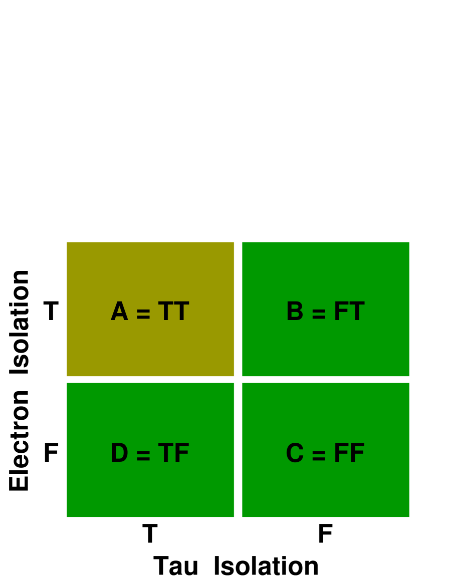
Figure 7.2: Using the uncorrelated tau isolation and electron isolation to estimate fake background for $\tau_{e}\tau_{h}$ channel.

Unfortunately, we can only cross check the fake background for $\tau_{e}\tau_{h}$ channel using the data sample from the CELE8 trigger path and possibly for $\tau_{\mu}\tau_{h}$ with CMUP muon channel using the data sample from the CMUP8 trigger path. Neither sample has isolation in the trigger. There is no such sample for $\tau_{\mu}\tau_{h}$ with CMX muon channel. There is a sample without isolation for $\tau_{h}\tau_{h}$ channel, but its prescale is 100 which is too large for this exercise.

Due to the statistics in the region B, C and D, this cross check can only be done for the $\tau_{e}\tau_{h}$ channel in the low mass control region. The numbers in region B, C and D are 12, 142 and 13, respectively. When we extrapolate to region A, we find that

$$\mbox{A}=\mbox{B}\times\mbox{D}/\mbox{C}=12\times 13/142=1.099$$ (7.11)

The normalization factor is 4.239, thus we get $\tau_{e}\tau_{h}$ fake extroplated = $1.099\times 4.239$ = 4.66. This is in good agreement with $3.83\pm 1.03$ obtained by summing up the weights of tau object being a jet. It does give us confidence in the method of the jet$\to\tau$ misidentified fake background estimate.

7.5 Uncertainties in Control Region

The statistical uncertainty and the systematic uncertainty of Drell-Yan background estimate include

• statistical uncertainty,

• $\sigma\cdot B$ uncertainty, 2%, aside from luminosity uncertainty (see Ref. [20]),

• trigger efficiencies (see Section 6.4),

• lepton scale factors (see Section 5.3.3 for $\tau$ scale factor, Section 5.4.2 for $e$ scale factor, and Section 5.5.2 for $\mu$ scale factors),

• $\,/\!\!\!\!E_{T}$ uncertainty, 6% (see Section 5.6), and

• luminosity, 6% (see Ref. [27]).

The statistical uncertainty and systematic uncertainty of the jet$\to\tau$ misidentified fake background estimate are discussed in Section 7.3.

We combine the $\tau_{\mu}\tau_{h}$ CMUP muon channel with a luminosity 195 pb^-1 and the $\tau_{\mu}\tau_{h}$ CMX muon channel with a luminosity 179 pb^-1 into one channel, simply called the $\tau_{\mu}\tau_{h}$ channel. The observed events in $\tau_{e}\tau_{h}$, $\tau_{\mu}\tau_{h}$ and $\tau_{h}\tau_{h}$ channels are 46, 36 and 8, respectively.

Table 7.4 shows the summary of the control sample in low mass region for 195 pb^-1 (72 pb^-1 for $\tau_{h}\tau_{h}$). The total background estimate is $99.27\pm 12.55$, dominated by the source from $Z/\gamma^{*}\to\tau\tau$ as expected. The observed number of events, 90, in the control region is in good agreement with this prediction. Fig. 7.3$-$7.5 show the distributions of each channel in the low mass control region. The observed distributions in the data are in good agreement with the predicted distributions.

Source	$\tau_{e}\tau_{h}$	$\tau_{\mu}\tau_{h}$	$\tau_{h}\tau_{h}$	Total
$Z/\gamma^{*}\to\tau\tau$	$45.36\pm 6.84$	$38.39\pm 5.72$	$4.19\pm 0.77$	$87.94\pm 12.38$
$Z/\gamma^{*}\to ee$	$0.14\pm 0.14$	0	0	$0.14\pm 0.14$
$Z/\gamma^{*}\to\mu\mu$	0	$0.48\pm 0.25$	0	$0.48\pm 0.25$
Jet$\to\tau$	$3.83\pm 1.03$	$3.72\pm 0.88$	$3.16\pm 0.55$	$10.71\pm 1.46$
Expected	$49.32\pm 6.94$	$42.59\pm 5.85$	$7.35\pm 0.95$	$99.27\pm 12.55$
Observed	46	36	8	90

Table 7.4: Number of expected events for each channel and each source, compared with the number observed, in the control region $m_{vis}<120$ GeV/$c^{2}$.

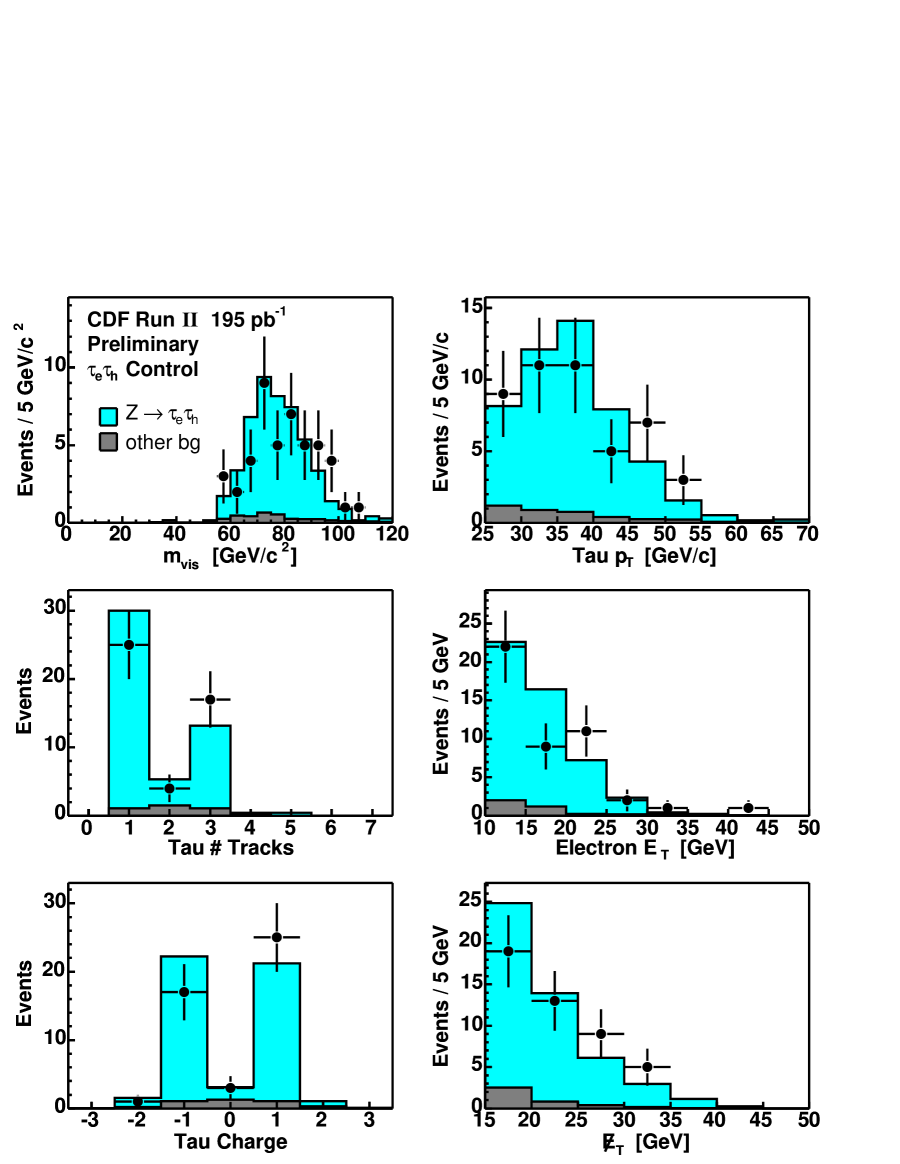
Figure 7.3: Distributions of the $\tau_{e}\tau_{h}$ channel in the control region for data (points) and predicted backgrounds (histograms).

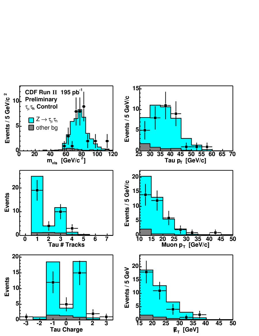
Figure 7.4: Distributions of the $\tau_{\mu}\tau_{h}$ channel in the control region for data (points) and predicted backgrounds (histograms).

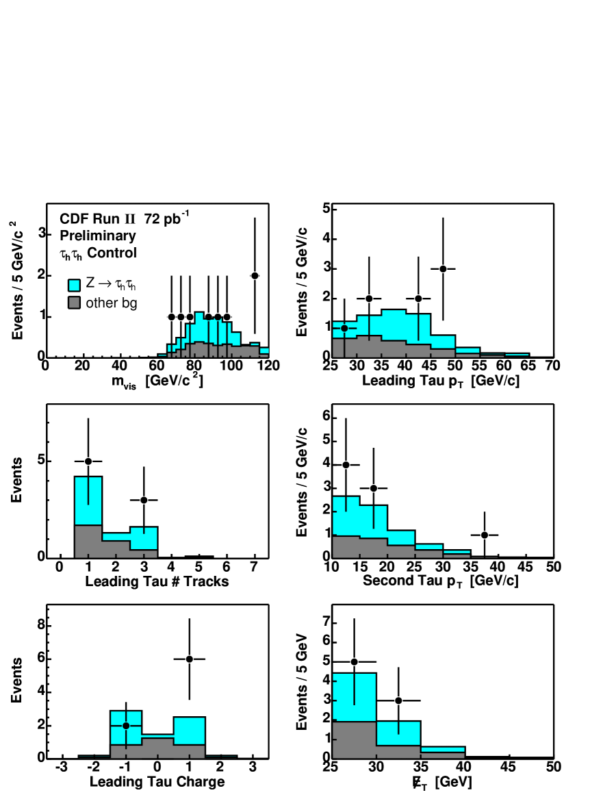
Figure 7.5: Distributions of the $\tau_{h}\tau_{h}$ channel in the control region for data (points) and predicted backgrounds (histograms).

Chapter 8 High Mass Signal Region

The high mass region with $m_{vis}>120$ GeV/$c^{2}$ is the signal region. First we calculate signal acceptance, then we estimate the backgrounds. The main backgrounds are $Z/\gamma^{*}\to\tau\tau$, $Z/\gamma^{*}\to ee$, $Z/\gamma^{*}\to\mu\mu$ which can be estimated from MC simulation, and the jet$\to\tau$ misidentified fake background which can be estimated from data, as in the control region.

8.1 Signal Acceptance

Table 8.1 shows the procedure to measure the signal acceptances in each channel for the new vector particle decaying to two taus, using $Z^{\prime}\to\tau\tau$ events. For example, for the $\tau_{e}\tau_{h}$ channel, we match the offline tau object and electron object with the $\tau_{h}$ and $\tau_{e}$ by requiring the separation angle be less than 0.2 radian, apply the event kinematic cuts, multiply the number of accepted events by the trigger efficiency and the lepton scale factors, and calculate the overall acceptance. Since the mass of the $Z^{\prime}$ is unknown, we calculate the signal acceptance as a function of its mass. Only five mass points (120, 180, 300, 450, 600) GeV/$c^{2}$ out of total twelve mass points (120, 140, 160, 180, 200, 250, 300, 350, 400, 450, 500, 600) GeV/$c^{2}$ are shown in Table 8.1. The signal acceptances of the $\tau_{\mu}\tau_{h}$ channel with a CMUP muon and of the $\tau_{\mu}\tau_{h}$ with a CMX muon are combined into one signal acceptance for the $\tau_{\mu}\tau_{h}$ channel. The total acceptance is a combination of the acceptance of the $\tau_{e}\tau_{h}$, the $\tau_{\mu}\tau_{h}$, and the $\tau_{h}\tau_{h}$ channels. The signal acceptances are shown in in Fig. 8.2.

Table 8.2 shows the procedure to measure the signal acceptances in each channel for the new scalar particle decaying to two taus, using $A\to\tau\tau$. We set $\tan\beta$ = 20 as a representative value of $\tan\beta$. Similarly, since the mass of $A$ is unknown, we calculate the signal acceptances as a function of mass, as shown in Fig. 8.2.

$Z^{\prime}\to\tau\tau$	m=120	m=180	m=300	m=450	m=600
event	100000	100000	100000	100000	100000
$\tau_{e}\tau_{h}$ (TAU_ELE)
$\tau_{e}\tau_{h}$ decay	23527	23209	23246	23345	23250
match $\tau(25)+e(10)$	761	1256	2135	2816	3044
$\,/\!\!\!\!E_{T}>15$	380	797	1720	2416	2745
$\Delta\phi(e-\,/\!\!\!\!E_{T})<30^{\circ}$	296	583	1231	1655	1844
$m_{vis}>120$	14	355	1125	1610	1814
trigger efficiency	12.9	327.0	1036.3	1483.1	1671.0
lepton scale factors	12.1	307.7	975.1	1395.4	1572.2
acceptance (%)	0.012	0.308	0.975	1.395	1.572
$\tau_{\mu}\tau_{h}$ (TAU_CMU)
$\tau_{\mu}\tau_{h}$ decay	22540	22500	22437	22358	22463
match $\tau(25)+\mbox{CMUP }\mu(10)$	418	698	1121	1492	1775
cosmic veto	418	698	1121	1491	1775
$\,/\!\!\!\!E_{T}>15$	198	460	894	1313	1615
$\Delta\phi(\mu-\,/\!\!\!\!E_{T})<30^{\circ}$	169	348	677	919	1134
$m_{vis}>120$	14	208	632	882	1114
trigger efficiency	12.8	189.6	576.1	804.0	1015.4
lepton scale factors	10.8	160.8	488.5	681.7	861.1
acceptance (%)	0.011	0.161	0.489	0.682	0.861
$\tau_{\mu}\tau_{h}$ (TAU_CMX)
$\tau_{\mu}\tau_{h}$ decay	22540	22500	22437	22358	22463
match $\tau(25)+\mbox{CMX }\mu(10)$	196	322	505	551	605
cosmic veto	196	322	505	551	605
$\,/\!\!\!\!E_{T}>15$	99	200	408	473	535
$\Delta\phi(\mu-\,/\!\!\!\!E_{T})<30^{\circ}$	88	140	301	345	379
$m_{vis}>120$	2	83	279	336	372
trigger efficiency	1.8	75.7	254.3	306.3	339.1
lepton scale factors	1.8	73.3	246.4	296.8	328.6
acceptance (%)	0.002	0.073	0.246	0.297	0.329
$\tau_{h}\tau_{h}$ (TAU_MET)
$\tau_{h}\tau_{h}$ decay	41677	41880	41934	41772	42027
match $\tau_{1}(25)+\tau_{2}(10)$	1662	2449	3415	3932	4257
$\,/\!\!\!\!E_{T}>25$	277	940	2037	2888	3383
$\Delta\phi(\tau_{2}-\,/\!\!\!\!E_{T})<30^{\circ}$	242	832	1679	2244	2459
$\tau_{2}$ num. track == 1	185	653	1335	1789	2043
$m_{vis}>120$	31	526	1282	1768	2028
trigger efficiency	21.2	388.3	1023.7	1469.1	1716.9
lepton scale factors	19.9	365.3	963.2	1382.3	1615.4
acceptance (%)	0.020	0.365	0.963	1.382	1.615
channels combined
acceptance (%)	0.045	0.907	2.673	3.756	4.377

Table 8.1: New vector particle $Z^{\prime}\to\tau\tau$ signal acceptance, for each channel, as a function of the $Z^{\prime}$ mass.

$A\to\tau\tau$	m=120	m=180	m=300	m=450	m=600
event	100000	100000	100000	100000	100000
$\tau_{e}\tau_{h}$ (TAU_ELE)
$\tau_{e}\tau_{h}$ decay	23427	23391	23364	23051	23242
match $\tau(25)+e(10)$	1063	1806	2556	2991	3375
$\,/\!\!\!\!E_{T}>15$	539	1237	2098	2665	3142
$\Delta\phi(e-\,/\!\!\!\!E_{T})<30^{\circ}$	396	870	1445	1723	2047
$m_{vis}>120$	23	547	1354	1684	2028
trigger efficiency	21.2	503.9	1247.3	1551.3	1868.1
lepton scale factors	19.9	474.1	1173.6	1459.6	1757.7
acceptance (%)	0.020	0.474	1.174	1.460	1.758
$\tau_{\mu}\tau_{h}$ (TAU_CMU)
$\tau_{\mu}\tau_{h}$ decay	22649	22759	22344	22472	22398
match $\tau(25)+\mbox{CMUP }\mu(10)$	650	1001	1454	1832	2076
cosmic veto	650	1000	1454	1832	2076
$\,/\!\!\!\!E_{T}>15$	353	671	1198	1634	1923
$\Delta\phi(\mu-\,/\!\!\!\!E_{T})<30^{\circ}$	286	492	855	1088	1272
$m_{vis}>120$	17	329	790	1063	1265
trigger efficiency	15.5	299.9	720.1	969.0	1153.1
lepton scale factors	13.1	254.3	610.6	821.6	977.8
acceptance (%)	0.013	0.254	0.611	0.822	0.978
$\tau_{\mu}\tau_{h}$ (TAU_CMX)
$\tau_{\mu}\tau_{h}$ decay	22649	22759	22344	22472	22398
match $\tau(25)+\mbox{CMX }\mu(10)$	239	407	552	601	612
cosmic veto	239	406	552	601	612
$\,/\!\!\!\!E_{T}>15$	120	297	449	522	553
$\Delta\phi(\mu-\,/\!\!\!\!E_{T})<30^{\circ}$	88	214	291	363	370
$m_{vis}>120$	6	138	266	355	365
trigger efficiency	5.5	125.8	242.5	323.6	332.7
lepton scale factors	5.3	121.9	235.0	313.6	322.4
acceptance (%)	0.005	0.122	0.235	0.314	0.322
$\tau_{h}\tau_{h}$ (TAU_MET)
$\tau_{h}\tau_{h}$ decay	41813	41837	42008	42104	41891
match $\tau_{1}(25)+\tau_{2}(10)$	2325	3117	3951	4333	4348
$\,/\!\!\!\!E_{T}>25$	495	1322	2534	3316	3653
$\Delta\phi(\tau_{2}-\,/\!\!\!\!E_{T})<30^{\circ}$	400	1072	1969	2467	2579
$\tau_{2}$ num. track == 1	293	821	1531	2005	2106
$m_{vis}>120$	46	630	1483	1985	2101
trigger efficiency	30.8	472.8	1202.9	1672.1	1789.5
lepton scale factors	29.0	444.9	1131.8	1573.3	1683.8
acceptance (%)	0.029	0.445	1.132	1.573	1.684
channels combined
acceptance (%)	0.067	1.295	3.151	4.168	4.742

Table 8.2: New scalar particle $A\to\tau\tau$ signal acceptance, for each channel, as a function of the $A$ mass.

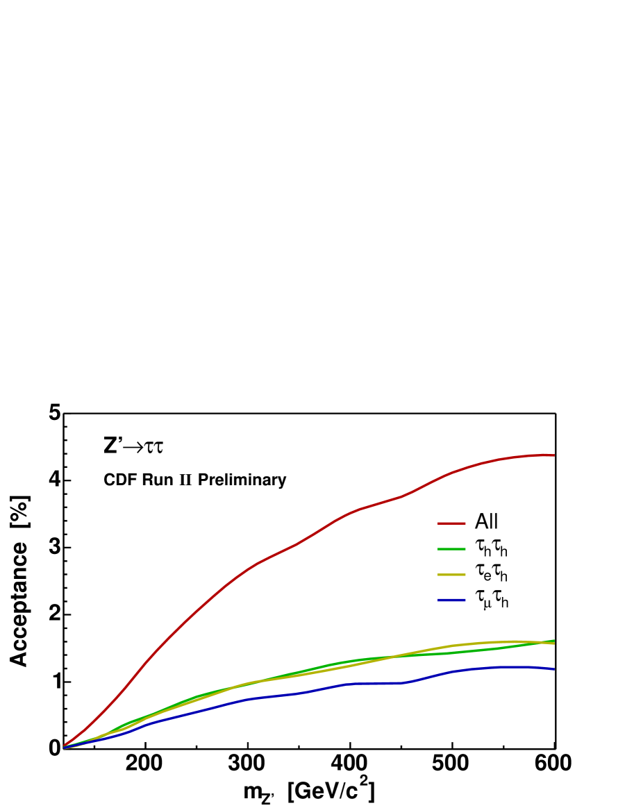
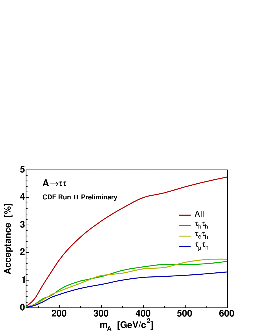
Figure 8.1: Signal acceptance of a new vector particle $Z^{\prime}\to\tau\tau$ in each channel, as a function of the $Z^{\prime}$ mass.

Figure 8.2: Signal acceptance of a new scalar particle $A\to\tau\tau$ in each channel, as a function of the $A$ mass.

8.2 Drell-Yan Background

The largest portion of the production cross section for the Drell-Yan backgrounds is at the $Z$ boson resonance peak, about 91 GeV/$c^{2}$. However the events in the high mass signal region are mostly from the high mass Drell-Yan tail. To model the high mass tail better, we need more statistics in MC simulation at that region. To achieve this, we break the generation level mass into two exclusively separated regions: $30<m<100$ GeV/$c^{2}$ and $m>100$ GeV/$c^{2}$, and simulate them separately. The production cross sections in these two regions are about 315 pb and 11 pb, respectively (see Section 7.1). Therefore we have a low-mass sample and a high-mass sample for each $Z/\gamma^{*}\to l^{+}l^{-}$ source.

Table 8.3 shows the procedure to estimate Drell-Yan backgrounds. We apply the event kinematic cuts on the MC samples, multiply the number of surviving events by the trigger efficiencies and the lepton scale factors, normalize to the integrated luminosity 195 pb^-1 (179 pb^-1 for the TAU_CMX trigger, 72 pb^-1 for the TAU_MET trigger), and combine the estimate for the low-mass Drell-Yan sample and the estimate for the high-mass Drell-Yan sample.

source	$Z/\gamma^{*}\to\tau\tau$		$Z/\gamma^{*}\to ee$		$Z/\gamma^{*}\to\mu\mu$
mass window	30$-$100	$>$100	30$-$100	$>$100	30$-$100	$>$100
$\sigma\cdot B$ (pb)	315	11	315	11	315	11
event	475901	160000	385686	160000	392063	160000
$\tau_{e}\tau_{h}$ (TAU_ELE)
$\tau(25)+e(10)$	1405	1062	257	190	1	1
$\,/\!\!\!\!E_{T}>15$	456	472	28	20	1	0
$\Delta\phi(e-\,/\!\!\!\!E_{T})<30^{\circ}$	381	364	2	2	0	0
$m_{vis}>120$	0	48	1	2	0	0
trigger efficiency	0.000	44.216	0.921	1.842	0.000	0.000
lepton scale factors	0.000	41.603	0.867	1.733	0.000	0.000
normalized (195 pb-1)	0.000	0.558	0.138	0.023	0.000	0.000
combined	0.56		0.16		0.00
$\tau_{\mu}\tau_{h}$ (TAU_CMU)
$\tau(25)+\mbox{CMUP }\mu(10)$	783	554	0	0	408	139
cosmic veto	783	554	0	0	408	139
$\,/\!\!\!\!E_{T}>15$	272	233	0	0	346	124
$\Delta\phi(\mu-\,/\!\!\!\!E_{T})<30^{\circ}$	238	179	0	0	7	0
$m_{vis}>120$	0	24	0	0	3	0
trigger efficiency	0.000	21.877	0.000	0.000	2.735	0.000
lepton scale factors	0.000	18.551	0.000	0.000	2.319	0.000
normalized (195 pb-1)	0.000	0.249	0.000	0.000	0.363	0.000
combined	0.25		0.00		0.36
$\tau_{\mu}\tau_{h}$ (TAU_CMX)
$\tau(25)+\mbox{CMX }\mu(10)$	384	284	0	0	212	49
cosmic veto	384	284	0	0	212	49
$\,/\!\!\!\!E_{T}>15$	127	129	0	0	174	41
$\Delta\phi(\mu-\,/\!\!\!\!E_{T})<30^{\circ}$	114	107	0	0	1	1
$m_{vis}>120$	0	23	0	0	1	1
trigger efficiency	0.000	20.965	0.000	0.000	0.912	0.912
lepton scale factors	0.000	20.318	0.000	0.000	0.883	0.883
normalized (179 pb-1)	0.000	0.250	0.000	0.000	0.127	0.011
combined	0.25		0.00		0.14
$\tau_{h}\tau_{h}$ (TAU_MET)
$\tau_{1}(25)+\tau_{2}(10)$	4023	2524	1	3	8	3
$\,/\!\!\!\!E_{T}>25$	249	428	0	0	0	2
$\Delta\phi(\tau_{2}-\,/\!\!\!\!E_{T})<30^{\circ}$	202	361	0	0	0	0
$\tau_{2}$ num. track == 1	158	269	0	0	0	0
$m_{vis}>120$	2	84	0	0	0	0
trigger efficiency	1.547	63.373	0.000	0.000	0.000	0.000
lepton scale factors	1.455	59.627	0.000	0.000	0.000	0.000
normalized (72 pb-1)	0.069	0.295	0.000	0.000	0.000	0.000
combined	0.36		0.00		0.00

Table 8.3: Drell-Yan background estimates for each channel in the high mass signal region.

8.3 Fake Background

The procedure to estimate the jet$\to\tau$ fake background is similar to what we have done for low mass control region in Section 7.3. The trigger path, the luminosity normalization factor, the denominator tau object definition, and the sum of the weights of tau objects being a jet in the high mass signal region are exactly the same as those in the low mass control region. The only one difference is this cut: $m_{vis}<120$ GeV/$c^{2}$ for the low mass control region, while $m_{vis}>120$ GeV/$c^{2}$ for the high mass signal region. Now we repeat the same procedure, as shown in Table 8.4. The event entries which are integers corresponding to the sum of weights which are real numbers are also shown. The event entries are used to estimate the statistical uncertainties.

channel	$\tau_{e}\tau_{h}$		CMUP $\tau_{\mu}\tau_{h}$		CMX $\tau_{\mu}\tau_{h}$		$\tau_{h}\tau_{h}$
trigger path	CELE8		CMUP8		TAU_CMX		TAU_MET
denominator	D_xi		D_xi		D_trkIso10Deg		D_xi
norm. factor	4.239		5.132		1		1
	$\sum\omega^{jet}$	event	$\sum\omega^{jet}$	event	$\sum\omega^{jet}$	event	$\sum\omega^{jet}$	event
$\sum\omega^{jet}$ or event	92.1	2292	12.4	362	64.4	379	106.8	2778
kinematic cuts	0.068	13	0.006	1	0.152	4	0.282	12
normalized	$0.29\pm 0.08$		$0.03\pm 0.03$		$0.15\pm 0.08$		$0.28\pm 0.08$

Table 8.4: Fake background estimates in the signal region. Uncertainties are statistical.

There is a systematic uncertainty due to the uncertainty in the jet$\to\tau$ fake rate. The rate used is the average fake rate of the JET samples. We use the individual fake rate of the JET20, JET50, JET70, and JET100 samples to estimate this uncertainty, as shown in Table 8.5.

channel	$\tau_{e}\tau_{h}$	CMUP $\tau_{\mu}\tau_{h}$	CMX $\tau_{\mu}\tau_{h}$	$\tau_{h}\tau_{h}$
average	0.29	0.03	0.15	0.28
JET20	0.18	0.03	0.16	0.31
JET50	0.23	0.04	0.15	0.23
JET70	0.31	0.03	0.14	0.25
JET100	0.28	0.03	0.13	0.22
syst. err	0.11	0.01	0.02	0.06

Table 8.5: Systematic uncertainties of fake background estimates in the signal region.

Combining in quadrature the statistical uncertainties in Table 8.4 and the systematic uncertainties in Table 8.5, we get

$$\tau_{e}\tau_{h}\mbox{ fake} = 0.29\pm 0.14$$ (8.1)

$$\mbox{CMUP }\tau_{\mu}\tau_{h}\mbox{ fake} = 0.03\pm 0.03$$ (8.2)

$$\mbox{CMX }\tau_{\mu}\tau_{h}\mbox{ fake} = 0.15\pm 0.08$$ (8.3)

$$\tau_{h}\tau_{h}\mbox{ fake} = 0.28\pm 0.10$$ (8.4)

8.4 Uncertainties in Signal Region

We summarize all of the systematic uncertainties in the high mass signal region in this section. Some of these are due to statistical uncertainties on the various backgrounds due to limited Monte Carlo or other statistics. Others come from separate external studies as indicated. And in this section, we combine the $\tau_{\mu}\tau_{h}$ with CMUP muon channel and the $\tau_{\mu}\tau_{h}$ with CMX muon channel into one single $\tau_{\mu}\tau_{h}$ channel.

The systematic uncertainty in the Drell-Yan and new particle signal rates due to the imperfect knowledge of the parton density functions (PDF’s) [22] is calculated by comparing the acceptance change ratio for various PDF’s. The CTEQ5L is used in PYTHIA. We add in quadrature the difference between MRST72 to CTEQ5L, MRST75 to MRST72, CTEQ6L1 to CTEQ6L, and CTEQ6M to CTEQ5L PDF’s. The MRST72 and MRST75 compare the effect of varying $\alpha_{s}$ on the PDF. The CTEQ5L set is leading order, and the CTEQ6M sets are next to leading order but at the same value of $\alpha_{s}$. Using $Z^{\prime}\to\tau\tau$, this is shown in Table 8.6. We take 8% as a conservative number.

$Z^{\prime}\to\tau\tau$	$m=120$	$m=180$	$m=300$	$m=400$	$m=600$
MRST72 / CTEQ5L	1.047	1.029	1.021	1.006	1.002
MRST75 / MRST72	0.951	0.980	0.983	0.995	0.993
CTEQ6L1 / CTEQ6L	1.006	1.006	1.003	0.999	1.002
CTEQ6M / CTEQ5L	1.035	1.023	1.021	1.008	1.004
PDF uncertainty	7.7%	4.2%	3.4%	1.1%	0.8%

Table 8.6: PDF uncertainty.

We are careful to identify the correlated and the uncorrelated systematic uncertainties. The correlated uncertainties include the uncertainties of the PDF, the integrated luminosity, the $e$, $\mu$, $\tau$ scale factors, the $\,/\!\!\!\!E_{T}$, and the jet$\to\tau$ fake rate. Table 8.7 lists the uncertainties, their magnitude, and the affected channels. (When uncertainties are correlated we assume a 100% correlation.)

Uncertainty	Magnitude (%)	Affected Channels
PDF	8	all
integrated luminosity	6	all
$e$ scale factor	4	$\tau_{e}\tau_{h}$
$\mu$ scale factor	5.5	$\tau_{\mu}\tau_{h}$
$\tau$ scale factor	10	all
$\,/\!\!\!\!E_{T}$	6	all
jet$\to\tau$ fake rate	20	all

Table 8.7: Systematic uncertainties, in percent, and the affected channels.

The $Z^{\prime}\to\tau\tau$ and $A\to\tau\tau$ signal acceptances and the systematic uncertainties are listed in Table 8.8$-$8.9. The acceptance itself reflects the effects of trigger efficiency and the lepton scale factors. The uncertainties include the contributions from

• statistical uncertainty (MC statistics),

• PDF uncertainty (this Section),

• trigger efficiencies (see Section 6.4),

• lepton scale factors (see Section 5.3.3 for $\tau$ scale factor, Section 5.4.2 for $e$ scale factor, and Section 5.5.2 for $\mu$ scale factors), and

• $\,/\!\!\!\!E_{T}$ uncertainty (see Section 5.6).

$m(Z^{\prime})$	$\tau_{e}\tau_{h}$ (%)	$\tau_{\mu}\tau_{h}$ (%)	$\tau_{h}\tau_{h}$ (%)	combined (%)
120	$0.012\pm 0.004$	$0.013\pm 0.004$	$0.020\pm 0.005$	$0.045\pm 0.009$
140	$0.084\pm 0.015$	$0.088\pm 0.015$	$0.105\pm 0.020$	$0.278\pm 0.043$
160	$0.213\pm 0.035$	$0.151\pm 0.025$	$0.206\pm 0.038$	$0.571\pm 0.086$
180	$0.308\pm 0.049$	$0.234\pm 0.037$	$0.365\pm 0.066$	$0.907\pm 0.136$
200	$0.453\pm 0.070$	$0.351\pm 0.054$	$0.476\pm 0.085$	$1.280\pm 0.190$
250	$0.727\pm 0.111$	$0.548\pm 0.083$	$0.776\pm 0.137$	$2.052\pm 0.30$3
300	$0.975\pm 0.148$	$0.735\pm 0.110$	$0.963\pm 0.170$	$2.673\pm 0.394$
350	$1.098\pm 0.167$	$0.826\pm 0.124$	$1.144\pm 0.202$	$3.068\pm 0.452$
400	$1.239\pm 0.188$	$0.966\pm 0.144$	$1.308\pm 0.230$	$3.512\pm 0.517$
450	$1.395\pm 0.211$	$0.979\pm 0.146$	$1.382\pm 0.243$	$3.756\pm 0.553$
500	$1.537\pm 0.232$	$1.148\pm 0.172$	$1.431\pm 0.252$	$4.116\pm 0.604$
600	$1.572\pm 0.237$	$1.190\pm 0.178$	$1.615\pm 0.284$	$4.377\pm 0.644$

Table 8.8: Uncertainties of $f\bar{f}\to Z^{\prime}\to\tau\tau$ signal acceptance (SM coupling).

$m(A)$	$\tau_{e}\tau_{h}$ (%)	$\tau_{\mu}\tau_{h}$ (%)	$\tau_{h}\tau_{h}$ (%)	combined (%)
120	$0.020\pm 0.005$	$0.018\pm 0.005$	$0.029\pm 0.007$	$0.067\pm 0.012$
140	$0.113\pm 0.019$	$0.082\pm 0.015$	$0.126\pm 0.024$	$0.321\pm 0.050$
160	$0.284\pm 0.045$	$0.213\pm 0.034$	$0.324\pm 0.058$	$0.822\pm 0.123$
180	$0.474\pm 0.074$	$0.376\pm 0.058$	$0.445\pm 0.079$	$1.295\pm 0.191$
200	$0.603\pm 0.093$	$0.485\pm 0.074$	$0.660\pm 0.117$	$1.748\pm 0.259$
250	$0.889\pm 0.135$	$0.703\pm 0.106$	$0.972\pm 0.172$	$2.564\pm 0.379$
300	$1.174\pm 0.178$	$0.846\pm 0.127$	$1.132\pm 0.199$	$3.151\pm 0.463$
350	$1.254\pm 0.190$	$1.004\pm 0.150$	$1.356\pm 0.239$	$3.614\pm 0.532$
400	$1.411\pm 0.213$	$1.101\pm 0.165$	$1.485\pm 0.261$	$3.996\pm 0.588$
450	$1.460\pm 0.220$	$1.135\pm 0.170$	$1.573\pm 0.277$	$4.168\pm 0.614$
500	$1.649\pm 0.249$	$1.177\pm 0.176$	$1.561\pm 0.275$	$4.386\pm 0.644$
600	$1.758\pm 0.265$	$1.300\pm 0.194$	$1.684\pm 0.296$	$4.742\pm 0.696$

Table 8.9: Uncertainties of $gg\to A\to\tau\tau$ signal acceptance ($\tan\beta=20$).

The systematic uncertainties on the Drell-Yan backgrounds and the jet$\to\tau$ misidentified fake backgrounds are listed in Table 8.10. The systematic uncertainties on the Drell-Yan backgrounds incorporate the effects of

• statistical uncertainty (MC statistics),

• PDF uncertainty (this Section),

• $\sigma\cdot B$ uncertainty, 2%, aside from luminosity uncertainty (see Ref. [20]),

• trigger efficiencies (see Section 6.4),

• lepton scale factors (see Section 5.3.3 for $\tau$ scale factor, Section 5.4.2 for $e$ scale factor, and Section 5.5.2 for $\mu$ scale factors),

• $\,/\!\!\!\!E_{T}$ uncertainty (see Section 5.6), and

• luminosity, 6% (see Ref. [27]).

The systematic uncertainties on the jet$\to\tau$ misidentified fake background incorporates the effects of

• statistical uncertainty (see Section 8.3), and

• systematic uncertainty due to jet$\to\tau$ misidentification rate (see Section 8.3).

Source	$\tau_{e}\tau_{h}$	$\tau_{\mu}\tau_{h}$	$\tau_{h}\tau_{h}$	Total
$Z/\gamma^{*}\to\tau\tau$	$0.56\pm 0.11$	$0.50\pm 0.10$	$0.36\pm 0.08$	$1.42\pm 0.23$
$Z/\gamma^{*}\to ee$	$0.16\pm 0.14$	0	0	$0.16\pm 0.14$
$Z/\gamma^{*}\to\mu\mu$	0	$0.50\pm 0.26$	0	$0.50\pm 0.26$
Jet$\to\tau$	$0.29\pm 0.14$	$0.18\pm 0.09$	$0.28\pm 0.10$	$0.75\pm 0.19$
Expected	$1.01\pm 0.24$	$1.18\pm 0.30$	$0.64\pm 0.13$	$2.83\pm 0.46$

Table 8.10: Uncertainties of backgrounds in signal region, 195 pb^-1 (72 pb^-1 for $\tau_{h}\tau_{h}$).

Chapter 9 Results

9.1 Observed Events

After unblinding the signal region, we observe four events in $\tau_{e}\tau_{h}$ channel, zero events in $\tau_{\mu}\tau_{h}$ channel, and zero events in $\tau_{h}\tau_{h}$ channel. The numbers of background events estimated and observed are in Table 9.1. Fig. 9.1 shows the $m_{vis}$ distribution. Fig. 9.2$-$9.5 shows the event displays of the four events observed in $\tau_{e}\tau_{h}$ channel.

Source	$\tau_{e}\tau_{h}$	$\tau_{\mu}\tau_{h}$	$\tau_{h}\tau_{h}$	Total
$Z/\gamma^{*}\to\tau\tau$	$0.56\pm 0.11$	$0.50\pm 0.10$	$0.36\pm 0.08$	$1.42\pm 0.23$
$Z/\gamma^{*}\to ee$	$0.16\pm 0.14$	0	0	$0.16\pm 0.14$
$Z/\gamma^{*}\to\mu\mu$	0	$0.50\pm 0.26$	0	$0.50\pm 0.26$
Jet$\to\tau$	$0.29\pm 0.14$	$0.18\pm 0.09$	$0.28\pm 0.10$	$0.75\pm 0.19$
Expected	$1.01\pm 0.24$	$1.18\pm 0.30$	$0.64\pm 0.13$	$2.83\pm 0.46$
Observed	4	0	0	4

Table 9.1: Number of expected events for each channel and each source, and number of observed events, in the signal region.

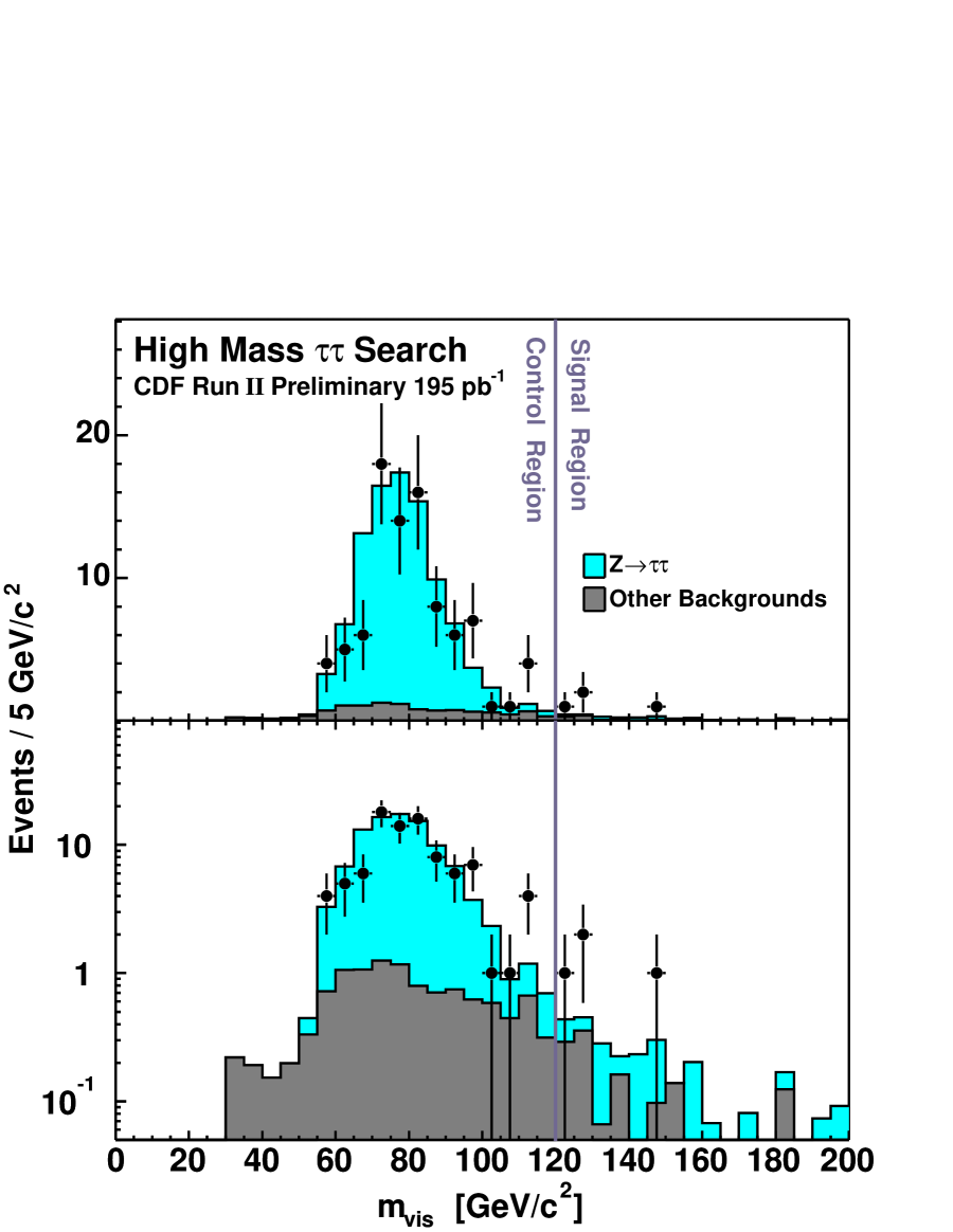
Figure 9.1: Distribution of visible mass ($m_{vis}$) for data (points) and predicted backgrounds (histograms) in the signal and control regions. The upper plot is in linear scale. The lower plot is in log scale.

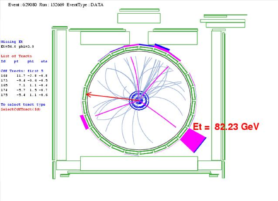
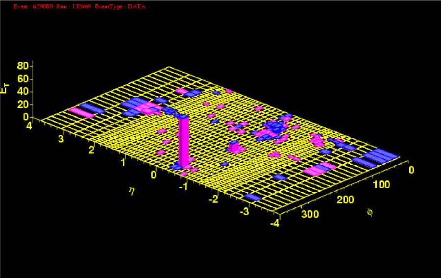
Figure 9.2: Event display $\tau_{e}\tau_{h}$ candidate run=152669 event=629080 $m_{vis}$=148 GeV/$c^{2}$.

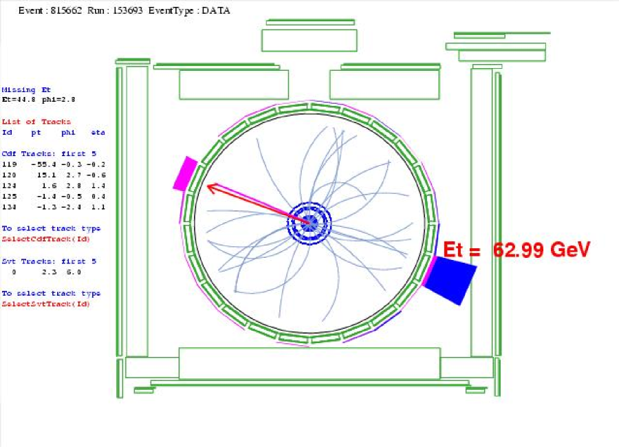
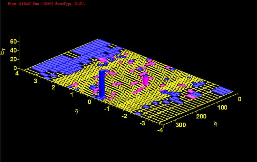
Figure 9.3: Event display $\tau_{e}\tau_{h}$ candidate run=153693 event=815662 $m_{vis}$=129 GeV/$c^{2}$.

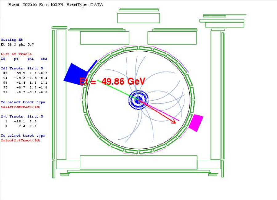
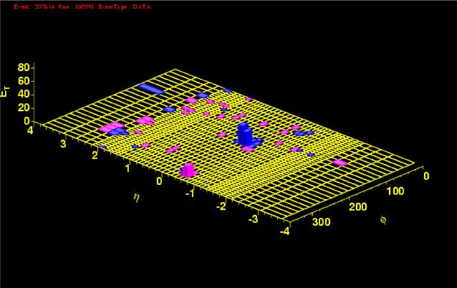
Figure 9.4: Event display $\tau_{e}\tau_{h}$ candidate run=160591 event=207616 $m_{vis}$=125 GeV/$c^{2}$.

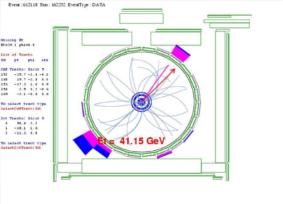
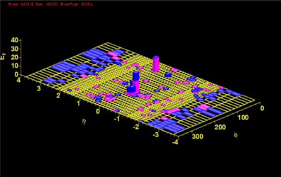
Figure 9.5: Event display $\tau_{e}\tau_{h}$ candidate run=162252 event=612118 $m_{vis}$=124 GeV/$c^{2}$.

9.2 Experimental Limits

Since we observe no excess, we proceed to calculate the 95% confidence level (CL) upper limit on the cross section times branching ratio for new particle production using a Bayesian procedure described in Ref. [38].

We need to combine multiple search channels and incorporate both uncorrelated and correlated systematic uncertainties. For each channel $i$, the integrated luminosity, the signal acceptance, the expected background events, and the observed events are denoted as $L_{i}$, $\epsilon_{i}$, $b_{i}$, and $n_{i}$, respectively; the uncorrelated uncertainties of the signal acceptance and the expected background events are denoted as $f_{\epsilon i}$ and $f_{bi}$, respectively. The correlated uncertainties of the integrated luminosity, the signal acceptance, and the expected background events are denoted as $g_{L}$, $g_{\epsilon}$, and $g_{b}$, respectively. (Note that the $f$ factors carry $i$ indices and the $g$ factors do not.) With a signal cross section $\sigma_{sig}$, the expected number of event $\mu_{i}$ in each channel can be written as

$$\mu_{i}=(1+g_{L})L_{i}\sigma_{sig}(1+f_{\epsilon i})(1+g_{\epsilon})\epsilon_{i}+(1+f_{bi})(1+g_{b})b_{i}$$ (9.1)

where the $f$ and $g$ factors are in a form $1+x$ thus relative systematic uncertainties. We define a likelihood which is the product of the Poisson probabilities of observing $n_{i}$ events in each channel,

$$\mathcal{L}(\bar{n}|\sigma_{sig},\bar{b},\bar{\epsilon})=\prod_{i}\mathcal{L}(n_{i}|\mu_{i})=\prod_{i}\frac{\mu_{i}^{n_{i}}e^{-\mu_{i}}}{n_{i}!}$$ (9.2)

where the overbars indicate that the variables are arrays carrying an $i$ index. We use a Monte Carlo method to convolute the effects of the systematic uncertainties using Gaussian prior probability density functions for the $f$ and $g$ factors. For an evaluating point of the $\sigma_{sig}$, we sample the $f$ and $g$ factors within their Gaussian widths around a central value of zero, calculate the $\mu_{i}$ and the $\mathcal{L}(n_{i}|\mu_{i})$ for each channel, and average the resulting likelihood $\mathcal{L}(\bar{n}|\sigma_{sig},\bar{b},\bar{\epsilon})$. Using Bayes’ Theorem, we then construct a probability density function for the signal cross section,

$$\mathcal{P}(\sigma_{sig}|\bar{n},\bar{b},\bar{\epsilon})=\frac{\mathcal{L}(n|\sigma_{sig},\bar{b},\bar{\epsilon})P(\sigma_{sig})}{\int_{0}^{\infty}\mathcal{L}(n|\sigma_{sig}^{\prime},\bar{b},\bar{\epsilon})P(\sigma_{sig}^{\prime})d\sigma_{sig}^{\prime}}$$ (9.3)

with a prior probability density function $P(\sigma_{sig})$ which expresses the subjective “degree of belief” for the value of the signal cross section. The 95% CL upper limit $\sigma_{95}$ is obtained by solving this integral equation

$$\int_{0}^{\sigma_{95}}\mathcal{P}(\sigma_{sig}|\bar{n},\bar{b},\bar{\epsilon})d\sigma_{sig}=0.95$$ (9.4)

We assume a uniform prior in the signal cross section up to some high cutoff; the value of the cutoff has no significant influence on the 95% CL upper limit.

We thereby extract the experimental 95% CL upper limit of $\sigma\cdot B$ for models using vector boson and scalar boson, respectively. The results are listed in Table 9.2 and shown in Fig. 9.6. These are the generic limits for $gg\to X_{\mbox{scalar}}\to\tau\tau$ and $f\bar{f}\to X_{\mbox{vector}}\to\tau\tau$ which can be interpreted in various models.

mass	vector	scalar
(GeV/$c^{2}$)	limit (pb)	limit (pb)
120	122.294	87.338
140	18.884	17.899
160	9.446	6.996
180	6.066	4.229
200	4.185	3.187
250	2.637	2.192
300	1.999	1.764
350	1.757	1.540
400	1.537	1.396
450	1.441	1.330
500	1.296	1.290
600	1.237	1.174

Table 9.2: The 95% CL upper limits on vector and scalar particle production and decay to tau pairs.

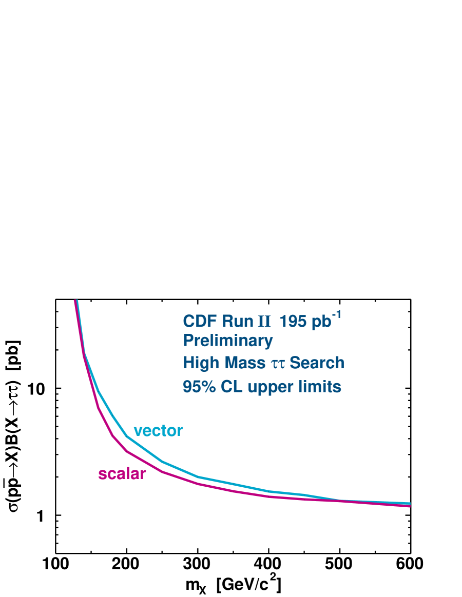
Figure 9.6: Upper limits at 95% CL on $\sigma(p\bar{p}\to X)B(X\to\tau\tau)$ for vector and scalar boson, as a function of mass.

9.3 Exclusion Regions

Now we can put the theoretical predictions on high mass tau pair production discussed in Section 2.3 and the experimental 95% CL upper limits together. We take the region where the theoretical prediction is bigger than the upper limit to be excluded at 95% CL.

For reference, this analysis would thus exclude at 95% CL a $Z^{\prime}$ with standard model couplings having a mass of less than 394 GeV/$c^{2}$, as shown in Fig. 9.7. For the MSSM pseudoscalar Higgs boson $A$, this analysis is not sensitive to exclude a region yet.

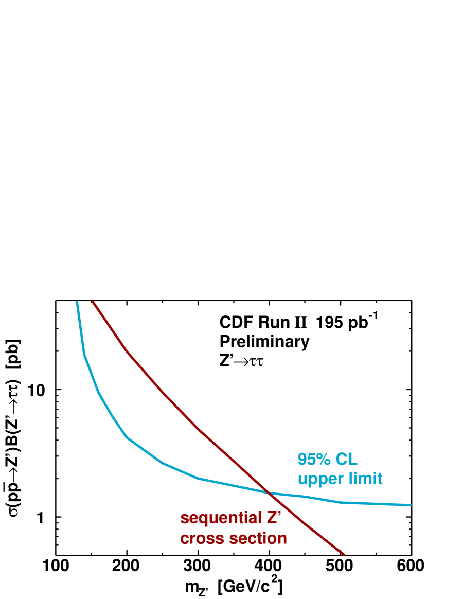
Figure 9.7: Upper limits at 95% CL and theoretical predictions of $\sigma(p\bar{p}\to Z^{\prime})B(Z^{\prime}\to\tau\tau)$. The excluded region is the region with $m(Z^{\prime})<394$ GeV/$c^{2}$.

Chapter 10 Conclusions

We have performed a blind search for high mass tau pairs using data corresponding to 195 pb^-1 of integrated luminosity from Run II of the Tevatron, using the CDF detector. In the high-mass region with $m_{vis}>120$ GeV/$c^{2}$, we expect $2.8\pm 0.5$ events from known background sources, and observe $4$ events in the data sample. Thus no significant excess is observed, and we use the result to set upper limits on the cross section times branching ratio to tau pairs of scalar and vector particles as a function of mass, shown in Table 9.2 and ploted in Fig. 9.6.

Chapter A The Structure of the Standard Model

The fundamental constituents of matter in Nature are fermions: leptons and quarks, with interactions specified by the gauge symmetries SU(3)_C$\times$SU(2)_L$\times$U(1)_Y in the framework of the Standard Model (SM).

Why are the fermions in an electroweak doublet? Why are left-handed fermions in a doublet, and right-handed fermions in a singlet? What tells us that quarks have color degrees-of-freedom? Why must quark doublets be paired with lepton doublets? Here we come to a brief review of how the structure of the SM emerged. A good introduction can be found in Ref. [39].

The relationships among the fermions are interpreted from the interactions they experience, namely the cross sections and decay widths measured, calculated, and measured … an interplay of experimental inputs and theoretical constraints. The objective is to unify the different interactions.

Charged Current

Let us recall Fermi’s theory [40] of charged current (CC) weak interaction for four fermions, e.g. the crossed $\beta$-decay, $ep\to n\nu_{e}$,

The amplitude (matrix element) of this process can be written as

$$\mathcal{M}=G_{F}J^{(e)\mu}J^{(p)}_{\mu}$$ (A.1)

where $G_{F}$ is Fermi’s constant and the charged currents for the fermion fields are

$$J^{(e)\mu}=\bar{u}_{e}\gamma^{\mu}u_{\nu_{e}},\;\;\;\;\;\;J^{(p)}_{\mu}=\bar{u}_{p}\gamma_{\mu}u_{n}$$ (A.2)

The next advance came after the discovery that CC violates parity maximally [41] and the V-A theory of the weak interaction [42] was proposed. Only left-handed fermions, which are projected by a V-A operator $\frac{1}{2}(1-\gamma_{5})$, appears in CC.

$$\mathcal{M}=\frac{4G}{\sqrt{2}}J_{\mu}^{\dagger}J^{\mu}$$ (A.3)

$$J^{\mu}=\bar{u}_{e}\gamma^{\mu}\frac{1}{2}(1-\gamma_{5})u_{\nu_{e}}+\bar{u}_{p}\gamma^{\mu}\frac{1}{2}(1-\gamma_{5})u_{n}$$ (A.4)

After the introduction of quarks [43] for understanding the classification of the hadrons, it was natural to re-write the hadronic part of CC in terms of quark fields. The transition $u\to d$ occurs via CC, with the other two quarks in the nucleon being spectators.

$$J^{\mu}=\bar{e}\gamma^{\mu}\frac{1}{2}(1-\gamma_{5})\nu_{e}+\bar{u}\gamma^{\mu}\frac{1}{2}(1-\gamma_{5})d^{\prime}$$ (A.5)

There was an inconsistency found in the value of the Fermi constant $G_{F}$ as determined from $\beta$-deay and the purely leptonic muon decay. This lead Cabibbo to the hypothesis that the quark states in CC are not the physical states (eigenstates of mass), but rather a quantum superposition of the physical states.

$$\left(\begin{array}[]{c}d\\ s\end{array}\right)_{\mbox{weak}}=\left(\begin{array}[]{cc}\cos\theta_{C}&\sin\theta_{C}\\ -\sin\theta_{C}&\cos\theta_{C}\end{array}\right)\left(\begin{array}[]{c}d\\ s\end{array}\right)_{\mbox{mass}}$$ (A.6)

where $\theta_{C}$ is Cabibbo angle, thus the Fermi constant is replaced by $G_{F}\cos\theta_{C}$. This idea was generalized to the case of three quark generations in terms of the CKM (Cabbibo-Kobayashi-Maskawa) matrix [5],

$$\left(\begin{array}[]{c}d\\ s\\ b\end{array}\right)_{\mbox{weak}}=\left(\begin{array}[]{ccc}V_{ud}&V_{us}&V_{ub}\\ V_{cd}&V_{cs}&V_{cb}\\ V_{td}&V_{ts}&V_{tb}\end{array}\right)\left(\begin{array}[]{c}d\\ s\\ b\end{array}\right)_{\mbox{mass}}$$ (A.7)

Glashow proposed the intermediate vector boson model (IVB) in 1961 [44] and the form has been incorportated in the SM. The basic idea is to replace the four fermion interaction by the exchange of a massive charged boson $W^{\pm}$, e.g. $\nu_{\mu}e^{-}\to\nu_{e}\mu^{-}$, (a) four fermion interaction, (b) the IVB model:

The matrix element can be written as

$$\mathcal{M}_{Fermi}^{CC}=\frac{4G_{F}}{\sqrt{2}}J_{\mu}^{CC}\left(J^{CC}\right)^{\mu}$$ (A.8)

$$\mathcal{M}_{IVB}^{CC}\approx\frac{g}{\sqrt{2}}J_{\mu}^{CC}\left(\frac{1}{m_{W}^{2}}\right)\frac{g}{\sqrt{2}}\left(J^{CC}\right)^{\mu}$$ (A.9)

Comparing Eq. (A.8) with Eq. (A.9), substituting $g=e/\sin\theta_{W}$ and $\alpha=e^{2}/(4\pi)$, and using experimental values: $\alpha=1/137$, $G_{F}=1.166\times 10^{-5}$ GeV^-2, $\sin^{2}\theta_{W}=0.22$ ($\sin^{2}\theta_{W}$ was first determined from the NC/CC cross section ratio in neutrino scattering where NC is the neutral current interaction explained below), this leads to the prediction for the W mass:

$$m_{W}=\left(\frac{\sqrt{2}g^{2}}{8G_{F}}\right)^{1/2}=\frac{37.3}{\sin\theta_{W}}=79.5\;\mbox{GeV}/c^{2}$$ (A.10)

This may be compared with the experimental value [3]:

$$m_{W}=80.425\pm 0.038\;\mbox{GeV}/c^{2}$$ (A.11)

The interdediate $W^{\pm}$ bosons, along with the $Z^{0}$ bosons explained below, were discovered at CERN in 1983 [45].

A Doublet in Weak Isospin Space

We write the left-handed leptons in a weak isospin SU(2)_L doublet and the right-handed leptons in a singlet, for example,

$$L=\left(\begin{array}[]{c}\nu_{e}\\ e_{L}^{-}\end{array}\right),\;\;\;e_{R}$$ (A.12)

The generators of the SU(2)_L transformations are $T_{L}^{i}=\frac{1}{2}\tau^{i}$, where $\tau^{i}$ are Pauli matrices. The charge raising opertator $\tau^{+}$, the charge lowering operator $\tau^{-}$, and the original $\tau^{3}$ are

$$\tau^{+} = \frac{1}{2}(\tau_{1}+i\tau_{2})=\left(\begin{array}[]{cc}0&1\\ 0&0\end{array}\right)$$ (A.15)

$$\tau^{-} = \frac{1}{2}(\tau_{1}-i\tau_{2})=\left(\begin{array}[]{cc}0&0\\ 1&0\end{array}\right)$$ (A.18)

$$\tau^{3} = \left(\begin{array}[]{cc}1&0\\ 0&-1\end{array}\right)$$ (A.21)

The currents can be written as

$$J_{\mu}^{+} = \bar{\nu}_{e}\gamma_{\mu}\frac{1}{2}(1-\gamma_{5})e\equiv\bar{\nu}_{e}\gamma_{\mu}e_{L}=\bar{L}\gamma_{\mu}\tau^{+}L$$ (A.22)

$$J_{\mu}^{-} = \bar{e}\gamma_{\mu}\frac{1}{2}(1-\gamma_{5})\nu_{e}\equiv\bar{e}_{L}\gamma_{\mu}\nu_{e}=\bar{L}\gamma_{\mu}\tau^{-}L$$ (A.23)

$$J_{\mu}^{3} = \frac{1}{2}\left[\bar{\nu}_{L}\gamma_{\mu}\nu_{L}-\bar{e}_{L}\gamma_{\mu}e_{L}\right]=\bar{L}\gamma_{\mu}\frac{1}{2}\tau^{3}L$$ (A.24)

These can be combined into an isospin triplet of currents

$$\mathbf{J}_{\mu}=\bar{L}\gamma_{\mu}\mathbf{T}L$$ (A.25)

The weak isospin invariance implies that the SU(2)_L invariant Lagrangian to describe the interaction between the $W$ bosons and the current $\mathbf{J}$ with a coupling $g$ is of the form

$$\mathcal{L}=g\mathbf{J}^{\mu}\cdot\mathbf{W}_{\mu}$$ (A.26)

Hence a neutral IVB W³ should exist, coupling to $J^{3}$. Since the electromagnetic current $J_{\mu}^{em}$ is parity conserving,

$$J_{\mu}^{em}=e(\bar{e}_{R}\gamma_{\mu}e_{R}+\bar{e}_{L}\gamma_{\mu}e_{L})$$ (A.27)

Whereas $J_{\mu}^{3}$ has a V-A structure. $J_{\mu}^{3}$ cannot be directly identified with the electromagnetic current, nor W³ with the photon.

Neutral Current

Next came the inputs from the neutral current (NC) interactions. NC were discovered by the Gargamelle Collaboration at CERN in 1973 [46], $\nu_{\mu}q\to\nu_{\mu}q$.

The matrix element can be written as

$$\mathcal{M}=\frac{8G_{F}\rho}{\sqrt{2}}\left(J^{NC}\right)^{\mu}J^{NC}_{\mu}$$ (A.28)

with NC in the form

$$\left(J^{NC}\right)^{\mu}=\sum_{l}\left[\bar{\nu}_{l}\gamma^{\mu}\frac{1}{2}(1-\gamma_{5})\nu_{l}\right]+\sum_{f}\left[\bar{f}\gamma^{\mu}\frac{1}{2}(C_{V}^{f}-C_{A}^{f}\gamma_{5})f\right]$$ (A.29)

$$l=e,\mu,\tau;\;\;\;f=l,q;\;\;\;q=u,d,s,c,b,t$$

The neutrino part has a V-A structure. The lepton/quark part has parity violation ($C_{A}^{f}\neq 0$), but not maximally ($C_{A}^{f}\neq C_{V}^{f}$). Universality of NC and CC requires $\rho=1$, later predicted in the SM.

We can write the NC interactions in terms of IVB, e.g. $\nu_{\mu}e^{-}\to\nu_{\mu}e^{-}$, (a) four fermion interaction, (b) the IVB model:

The matrix element can be written as

$$\mathcal{M}_{Fermi}^{NC}=\frac{8\rho G_{F}}{\sqrt{2}}J_{\mu}^{NC}\left(J^{NC}\right)^{\mu}$$ (A.30)

$$\mathcal{M}_{IVB}^{NC}\approx\frac{g}{\cos\theta_{W}}J_{\mu}^{NC}\left(\frac{1}{m_{Z}^{2}}\right)\frac{g}{\cos\theta_{W}}\left(J^{NC}\right)^{\mu}$$ (A.31)

Comparing Eq. (A.30) with Eq. (A.31), and assuming universality of the charged and neutral currents ($\rho=1$), this gives the prediction for Z mass:

$$m_{Z}=\left(\frac{\sqrt{2}g^{2}}{8G_{F}}\right)^{1/2}\frac{1}{\sqrt{\rho}\cos\theta_{W}}=\frac{m_{W}}{\sqrt{\rho}\cos\theta_{W}}=\frac{79.5}{\cos\theta_{W}}=90\;\mbox{GeV}/c^{2}$$ (A.32)

This may be compared with the experimental value [3]:

$$m_{Z}=91.1876\pm 0.0021\;\mbox{GeV}/c^{2}$$ (A.33)

Flavor Changing Neutral Current

The flavor changing neutral current (FCNC) interaction is strongly suppressed [3], (a) CC, (b) FCNC:

$$J^{NC}=\bar{u}u+\bar{d}^{\prime}d^{\prime}=\bar{u}u+\bar{d}d\cos^{2}\theta_{C}+\bar{s}s\sin^{2}\theta_{C}+\underbrace{(\bar{s}d+\bar{d}s)}_{\mbox{FCNC}}\sin\theta_{C}\cos\theta_{C}$$ (A.34)

$$\mbox{BR}(K^{+}\to\pi^{+}\pi^{0}) = (21.13\pm 0.14)\%$$ (A.35)

$$\mbox{BR}(K^{+}\to\pi^{+}e^{+}e^{-}) = (2.88\pm 0.13)\times 10^{-7}$$ (A.36)

The GIM (Glashow-Iliopoulos-Maiani) mechanism [47] proposed that quarks must be paired in doublets. This naturally solved FCNC. In addition, $c$ quark was predicted and later discovered [48].

$$\left(\begin{array}[]{c}u\\ d^{\prime}\end{array}\right)\;\;\;\left(\begin{array}[]{c}c\\ s^{\prime}\end{array}\right)$$ (A.37)

$$J^{NC}=\bar{u}u+\bar{c}c+\bar{d}^{\prime}d^{\prime}+\bar{s}^{\prime}s^{\prime}=\bar{u}u+\bar{c}c+\bar{d}d+\bar{s}s$$ (A.38)

A Triplet in Quark Color Space

The quarks in the spin-$\frac{3}{2}$ baryons are in a symmetrical state of space, spin and flavor degrees of freedom, e.g.

$$\Delta^{++}=uuu,\;\;\;\;\;\;\Omega^{-}=sss$$ (A.39)

However the requirements of Fermi-Dirac statistics imply the total antisymmetry of the wave function. The solution was the introduction of the color degree of freedom, with indices as red ($r$), green ($g$), and blue ($b$).

$$q=\left(\begin{array}[]{c}q_{r}\\ q_{g}\\ q_{b}\end{array}\right)$$ (A.40)

One of the tests of the number of charged fundamental constituents is provided by

$$R=\frac{\sigma(e^{+}e^{-}\to\mbox{hadrons})}{\sigma(e^{+}e^{-}\to\mu^{+}\mu^{-})}$$ (A.41)

The virtual photon emitted by the $e^{+}e^{-}$ annihilation will excite all kinematically accessible $q\bar{q}$ pairs from the vacuum.

$$R=\sum_{q}e_{q}^{2}$$ (A.42)

At low energy where only the $u$, $d$ and $s$ quarks are available, in the absense of color degree of freedom, we expect

$$R=e_{u}^{2}+e_{d}^{2}+e_{s}^{2}=\left(\frac{2}{3}\right)^{2}+\left(-\frac{1}{3}\right)^{2}+\left(-\frac{1}{3}\right)^{2}=\frac{2}{3}$$ (A.43)

If quarks have three colors,

$$R=3(e_{u}^{2}+e_{d}^{2}+e_{s}^{2})=2$$ (A.44)

For energies above 10 GeV, $c$ and $b$ quarks are available,

$$R=3(e_{u}^{2}+e_{d}^{2}+e_{s}^{2}+e_{c}^{2}+e_{b}^{2})=\frac{11}{3}$$ (A.45)

The color triplet model is excellently supported by data, see the “$\sigma$ and $R$ in $e^{+}e^{-}$ Collisions” plots in the Section “Plots of cross sections and related quantities (Rev.)” in PDG [3].

Pair Quarks with Leptons

Some classical symmetries, known as anomalous symmetries [49] are broken by quantum effects. The requirement for an anomaly-free theory [50] is that:

$$\sum Q_{f}=0$$ (A.46)

where the sum is over all quarks and leptons. For example consider the two doublets,

$$\left(\begin{array}[]{c}\nu_{e}\\ e\end{array}\right)$$ (A.49)

$$\left(\begin{array}[]{c}u\\ d\end{array}\right)$$ (A.52)

$$\sum Q_{f}=(0-1)+3\times(\frac{2}{3}-\frac{1}{3})=0$$ (A.53)

Cancellation of anomalies requires that quark doublets must be paired with lepton doublets. The SM identifies a generation in a natural way by identifying the doublet containing the heaviest charged lepton with the doublet containing the heaviest quarks (and so on), but one could in principle associate any quark doublet with any lepton doublet and call that a generation, because there are no interactions between quarks and leptons in the SM. What needs to be guaranteed is that the number of quark and lepton generations must be equal.

Chapter B Gauge Symmetry & Spontaneous Symmetry Breaking

The interactions between the fermions and the vector bosons in the Standard Model (SM) are uniquely specified by requiring the theory, i.e. the SM Lagrangian, invariant under gauge transformations which are local and involve transformations varying from point to point. Some of the standard texts are listed in Ref. [51].

A symmetry indicates a deeper relationship among the elementary particles with a further unification of the interactions and makes the form of a Lagrangian more compact. Symmetry dictates design and plays the central role in the direction to find the simplest model.

Gauge Symmetry

Let us take electromagnetism as an example and consider the Lagrangian for a free fermion field $\Psi(x)$.

$$\mathcal{L}_{0}=\bar{\Psi}(x)(i\gamma^{\mu}\partial_{\mu}-m)\Psi(x)$$ (B.1)

This is invariant under a global U(1) phase transformation which is space-time independent and is illustrated in the left plot in Fig. B.1,

$$\Psi(x)\to\Psi^{\prime}(x)=e^{-iQ\theta}\Psi(x)$$ (B.2)

where $Q$ is the charge or the U(1) quantum number of the fermion. For example, the charge assignment for $u$ quark, $d$ quark, $\nu_{e}$, and $e$ are +2/3, -1/3, 0, and -1, respectively.

We are going to construct an invariant Lagrangian under a local, i.e., gauge, U(1) phase transformation which is space-time dependent and is illustrated in the right plot in Fig. B.1.

$$\Psi(x)\to\Psi^{\prime}(x)=e^{-iQ\theta(x)}\Psi(x)$$ (B.3)

The partial derivative $\partial_{\mu}$ in Eq. (B.1) spoils the invariance. We need to form a gauge-covariant derivative $D_{\mu}$ which will have the simple transformation property,

$$D_{\mu}\Psi(x)\to e^{-iQ\theta(x)}D_{\mu}\Psi(x)$$ (B.4)

so that the combination $\bar{\Psi}D_{\mu}\Psi$ is gauge invariant. To achieve this, we enlarge the Lagrangian with a new vector gauge field $A_{\mu}(x)$ and form the covariant form as

$$D_{\mu}\Psi=(\partial_{\mu}+ieQA_{\mu})\Psi$$ (B.5)

where $e$ is a free parameter which eventually will be identified as the coupling of the gauge field to the fermion field. The transformation property in Eq. (B.4) will be satisfied if the gauge field $A_{\mu}(x)$ has the transformation property

$$A_{\mu}(x)\to A^{\prime}_{\mu}(x)=A_{\mu}(x)+\frac{1}{e}\partial_{\mu}\theta(x)$$ (B.6)

Note that the coupling of the gauge field (photon) to any fermion field is determined by its transformation property under the symmetry group. This is usually referred to as universality. Also note that photon is massless because an $A_{\mu}A^{\mu}$ term is not gauge invariant under this transformation.

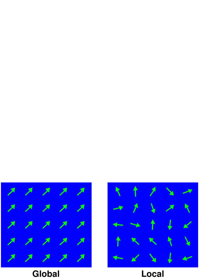
Figure B.1: Global and local transformations.

To make the photon field a truely dynamical variable we need to add a kinetic term to the Lagrangian involving its derivatives. The simplest gauge-invariant term with a conventional normalization is

$$\mathcal{L}_{A}=-\frac{1}{4}F_{\mu\nu}F^{\mu\nu}$$ (B.7)

where

$$F_{\mu\nu}=\partial_{\mu}A_{\nu}-\partial_{\nu}A_{\mu}$$ (B.8)

Terms with higher powers are omitted in order that the theory be renormalizable. We notice that photon does not have self-coupling because it does not carry a charge.

Now we arrive at the gauge-invariant QED Lagrangian

$$\mathcal{L}_{QED}=\bar{\Psi}i\gamma^{\mu}(\partial_{\mu}+ieQA_{\mu})\Psi-m\bar{\Psi}\Psi-\frac{1}{4}F_{\mu\nu}F^{\mu\nu}$$ (B.9)

Most remarkably, if one demands the symmetry be local, one is forced to include the electromagnetic field, and hence, light. Recall that there are four Maxwell equations. While here we just require “gauge symmetry” and electromagnetism is determined. This illustrates how physics becomes simpler.

Non-Abelian Gauge Symmetry

Yang and Mills extended the gauge principle to non-Abelian symmetry [52]. Consider the simplest case isospin SU(2). Let the fermion field be an isospin doublet,

$$\Psi=\left(\begin{array}[]{c}\Psi_{1}\\ \Psi_{2}\end{array}\right)$$ (B.10)

The free Lagragian

$$\mathcal{L}_{0}=\bar{\Psi}(x)(i\gamma^{\mu}\partial_{\mu}-m)\Psi(x)$$ (B.11)

is invariant under the global SU(2) transformation

$$\Psi(x)\to\Psi^{\prime}(x)=e^{-i\mathbf{T}\cdot\mathbf{\theta}}\Psi(x)$$ (B.12)

where $\mathbf{\theta}=(\theta_{1},\theta_{2},\theta_{3})$ are the SU(2) transformation parameters and $\mathbf{T}=\frac{\mathbf{\tau}}{2}$ are the SU(2) generators with $\mathbf{\tau}=(\tau_{1},\tau_{2},\tau_{3})$ the Pauli matrices satisfying

$$[T_{i},T_{j}]=i\epsilon_{ijk}T_{k}\;\;\;\;\;\;i,j,k=1,2,3$$ (B.13)

with $\epsilon_{ijk}$ the structure constants for SU(2).

It is easy to check that two successive SU(2) transformations do not commute because the generators do not commute and this is why SU(2) is called a non-Abelian symmetry, in contrast to an Abelian symmetry such as U(1) where two successive U(1) transformations commute.

Under the local symmetry transformation

$$\Psi(x)\to\Psi^{\prime}(x)=e^{-i\mathbf{T}\cdot\mathbf{\theta}(x)}\Psi(x)$$ (B.14)

the partial derivative $\partial_{\mu}$ in Eq. (B.11) spoils the invariance. To construct a gauge-invariant Lagrangian we follow a procedure similar to that of the Abelian case:

• We form a gauge-covariant derivative

  $$D_{\mu}\Psi(x)\to e^{-i\mathbf{T}\cdot\mathbf{\theta}(x)}D_{\mu}\Psi(x)$$ (B.15)

  by introducing vector gauge fields $A_{\mu}^{i}$, $i=1,2,3$ (one for each group generator) and a coupling $g$

  $$D_{\mu}\Psi=(\partial_{\mu}+ig\mathbf{T}\cdot\mathbf{A}_{\mu})\Psi$$ (B.16)

  and defining the transformation property for the vector gauge fields as,

  $$A_{\mu}^{i}\to A_{\mu}^{i^{\prime}}=A_{\mu}^{i}-\epsilon^{ijk}\theta^{j}A_{\mu}^{k}+\frac{1}{g}\partial_{\mu}\theta^{i}$$ (B.17)

  The gauge fields are massless because an $A_{\mu}^{i}A^{i\mu}$ term is not gauge invariant, similar to an Abelian field. But, the second term is clearly the transformation for a triplet representation under SU(2), thus the $A_{\mu}^{i}$ fields carry charges.

• Then we add a gauge invariant kinetic term for the gauge fields

  $$\mathcal{L}_{A}=-\frac{1}{4}F_{\mu\nu}^{i}F^{i\mu\nu}$$ (B.18)

  where

  $$F_{\mu\nu}^{i}=\partial_{\mu}A_{\nu}^{i}-\partial_{\nu}A_{\mu}^{i}-g\epsilon^{ijk}A_{\mu}^{j}A_{\nu}^{k}$$ (B.19)

  The third term shows that the gauge fields have self-coupling because they carry charge, in contrast to an Abelian field.

We arrive at the complete gauge-invariant Lagrangian which describes the interaction between the gauge fields $A_{\mu}^{i}$ and the SU(2) doublet fields,

$$\mathcal{L}=\bar{\Psi}i\gamma^{\mu}(\partial_{\mu}+ig\mathbf{T}\cdot\mathbf{A}_{\mu})\Psi-m\bar{\Psi}\Psi-\frac{1}{4}F_{\mu\nu}^{i}F^{i\mu\nu}$$ (B.20)

Generalization of the Yang-Mills theory to a higher group SU(N) with $N\geq 3$ is straightforward.

SU(3)_C$\times$SU(2)_L$\times$U(1)_Y

The structure of the gauge symmetries in the SM is SU(3)_C$\times$SU(2)_L$\times$U(1)_Y. For a particular fermion $\Psi$, its quantum field is a product of factors,

$$\Psi=\left(\begin{array}[]{c}\mbox{space-time}\\ \mbox{factor}\end{array}\right)\times\left(\begin{array}[]{c}\mbox{spin}\\ \mbox{factor}\end{array}\right)\times\left(\begin{array}[]{c}\mbox{U(1)}_{Y}\\ \mbox{factor}\end{array}\right)\times\left(\begin{array}[]{c}\mbox{SU(2)}_{L}\\ \mbox{factor}\end{array}\right)\times\left(\begin{array}[]{c}\mbox{SU(3)}_{C}\\ \mbox{factor}\end{array}\right)$$ (B.21)

Each factor has some labels, coordinates, or indices. The orthonormality of the quantum field holds separately for each factor. Since the gauge bosons of one of the symmetry groups do not transform under the other gauge symmetries in the product of groups, the gauge invariant Lagrangian may be simply written as a sum of the terms of individual groups. The gauge symmetric Lagrangian in the framework of Yang-Mills theory is

$$\mathcal{L}_{symmetric} = \bar{\Psi}i\gamma^{\mu}\left(\partial_{\mu}+ig_{1}\frac{Y}{2}B_{\mu}+ig_{2}T^{j}W_{\mu}^{j}+ig_{3}\lambda^{a}G_{\mu}^{a}\right)\Psi$$

$$-\frac{1}{4}B_{\mu\nu}B^{\mu\nu}-\frac{1}{4}W_{\mu\nu}^{i}W^{i\mu\nu}-\frac{1}{4}G_{\mu\nu}^{a}G^{a\mu\nu}$$

where the eight $G_{\mu}^{a}$ and $\lambda^{a}$, the three $W_{\mu}^{i}$ and $T^{i}$, the one B_μ and $Y$ are the gauge bosons and generators corresponding to the SU(3)_C color, the SU(2)_L weak isospin, and the U(1)_Y hypercharge gauge symmetries, respectively; $g_{i}$ are the gauge couplings; and

$$B_{\mu\nu} = \partial_{\mu}B_{\nu}-\partial_{\nu}B_{\mu}$$ (B.23)

$$W_{\mu\nu}^{i} = \partial_{\mu}W_{\nu}^{i}-\partial_{\nu}W_{\mu}^{i}+g_{2}\epsilon^{ijk}W_{\mu}^{j}W_{\nu}^{k}$$ (B.24)

$$G_{\mu\nu}^{a} = \partial_{\mu}G_{\nu}^{a}-\partial_{\nu}G_{\mu}^{a}+g_{3}f^{abc}G_{\mu}^{b}G_{\nu}^{c}$$ (B.25)

with $\epsilon^{ijk}$ and $f^{abc}$ the structure constants for SU(2) and SU(3).

At this stage, all of the gauge bosons and fermions are massless. The explicit mass terms break gauge invariance. For gauge bosons, the exptected mass terms

$$m_{W}^{2}W_{\mu}W^{\mu}$$ (B.26)

plus similar terms for the others, are clearly not invariant under gauge transformations $W_{\mu}^{i}\to W_{\mu}^{i^{\prime}}=W_{\mu}^{i}-\epsilon^{ijk}\theta^{j}W_{\mu}^{k}+\frac{1}{g_{2}}\partial_{\mu}\theta^{i}$. This is true for any gauge theory. For fermions, using the left- and right-handed projection operator $P_{L}$ and $P_{R}$, the mass term can be written as

$$m\bar{\Psi}\Psi = m\bar{\Psi}(P_{L}+P_{R})\Psi$$ (B.27)

$$= m\bar{\Psi}P_{L}P_{L}\Psi+m\bar{\Psi}P_{R}P_{R}\Psi$$

$$= m(\bar{\Psi}_{R}\Psi_{L}+\bar{\Psi}_{L}\Psi_{R})$$

In the SM, left-handed fermions are in SU(2) doublets and the right-handed fermions are in SU(2) singlets, thus they transform differently. The $\bar{\Psi}_{R}\Psi_{L}$ and $\bar{\Psi}_{L}\Psi_{R}$ terms are not SU(2) singlets and would not give an SU(2) invariant Lagrangian.

However the description that all of the gauge bosons and fermions are massless is not true in Nature. We need to

• generate the masses of the leptons and quarks;

• generate the masses of the $W^{+}$, $W^{-}$, and $Z^{0}$ weak vector bosons;

• but also keep the photon and gluon massless.

In other words, the SU(3)_C will be kept precise, and the gluon will remain massless. We need to break SU(2)_L$\times$U(1)_Y down to U(1)_EM, resulting in mixing between the $B_{\mu}$ and $W_{\mu}^{3}$ fields, and non-zero masses for three of the gauge bosons ($W^{\pm}$ and $Z^{0}$). The photon ($A$) remain massless, due to a residual U(1)_EM gauge symmetry that remains unbroken.

Spontaneous Symmetry Breaking

The solution in the SM is to add a spontaneous symmetry breaking (SSB) term into the symmetric Lagrangian “by hand”. The Lagrangian will remain symmetric but the physical vacuum does not respect the symmetry. In this case, the symmetry of the Lagrangian is said to be spontaneously broken.

$$\mathcal{L}=\mathcal{L}_{symmetric}+\mathcal{L}_{SSB}$$ (B.28)

The assumption to construct $\mathcal{L}_{SSB}$ is that the universe is filled with a scalar field, called Higgs field. One real scalar field could solve (a). One complex field could solve (a) and create one massive vector boson. To achieve (a), (b) and (c), the minimum requirement of the Higgs field is two complex fields arranged in a doublet in the SU(2) space and carries U(1) hypercharge +1 (electric charge $Q=T_{L}^{3}+\frac{Y}{2}$ is +1 and 0 for the upper and lower component, respectively), but is a singlet in color space.

$$\phi=\left(\begin{array}[]{c}\phi^{+}\\ \phi^{0}\end{array}\right)=\frac{1}{\sqrt{2}}\left(\begin{array}[]{c}\phi_{1}+i\phi_{2}\\ \phi_{3}+i\phi_{4}\end{array}\right)$$ (B.29)

Under a SU(2)_L$\times$U(1)_Y gauge transformation, the doublet transforms as

$$\phi\to e^{-i\frac{1}{2}\alpha(x)}e^{-iT^{i}\beta^{i}(x)}\phi$$ (B.30)

The scalar field can be given gauge invariant terms in $\mathcal{L}_{SSB}$: the kinetic term required by gauge invariance, the Higgs potential including a mass-like term and a self-interaction term, and the Yukawa coupling between the doublet and a particular fermion $\Psi$.

$$\mathcal{L}_{SSB}=(D_{\mu}\phi)^{\dagger}(D^{\mu}\phi)-V(\phi)-\mathcal{L}_{Yukawa}$$ (B.31)

with

$$D_{\mu} = \partial_{\mu}+ig_{1}\frac{1}{2}B_{\mu}+ig_{2}T^{j}W_{\mu}^{j}$$ (B.32)

$$V(\phi) = \mu^{2}\phi^{\dagger}\phi+\lambda\left(\phi^{\dagger}\phi\right)^{2}$$ (B.33)

$$\mathcal{L}_{Yukawa} = g_{f}\bar{\Psi}\phi\Psi$$ (B.34)

Spontaneous symmetry breaking of the Higgs potential [4] is possible by assuming $\mu^{2}<0$ (also a positive $\lambda$ to possess a stable vacuum). This is shown in Fig. B.2.

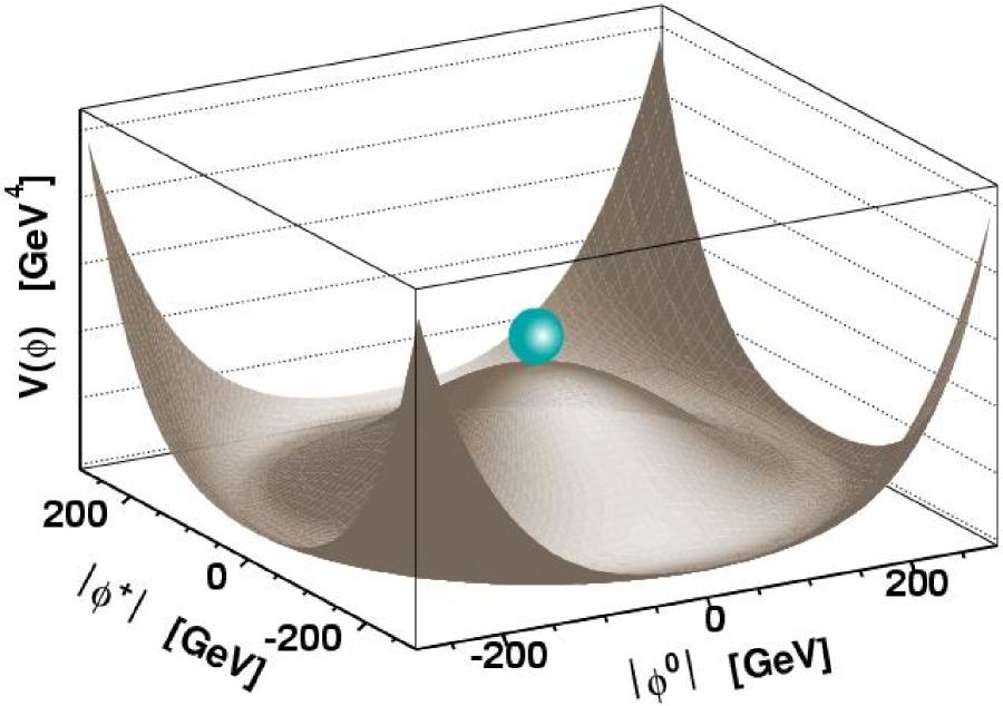
Figure B.2: Spontaneous symmetry breaking of Higgs potential.

The minimum of the Higgs potential shifts (in field space) from $\phi=0$ to

$$\phi^{\dagger}\phi=\frac{1}{2}\left(\phi_{1}^{2}+\phi_{2}^{2}+\phi_{3}^{2}+\phi_{4}^{2}\right)=\frac{-\mu^{2}}{\lambda}=v^{2}$$ (B.35)

The field thus acquires a non-zero vacuum expectation value (VEV). Choosing $\langle\phi^{3}\rangle=v$, we expand about $v$,

$$\phi=\frac{1}{\sqrt{2}}\left(\begin{array}[]{c}\phi_{1}+i\phi_{2}\\ v+H+i\phi_{4}\end{array}\right)$$ (B.36)

with $\phi^{3}=v+H$. Any SU(2) doublet can be written as

$$\phi=\left(e^{-iT^{i}\theta^{i}(x)}\right)^{\dagger}\left(\begin{array}[]{c}0\\ \sigma(x)\end{array}\right)$$ (B.37)

By applying the gauge symmetry of $\mathcal{L}_{SSB}$ under the transformation of the Higgs doublet in Eq. (B.30), the algebra can be simplied by “gauging away” three of the four real degrees of freedom of the Higgs doublet with $\phi^{1},\phi^{2},\phi^{4}=0$,

$$\phi=\frac{1}{\sqrt{2}}\left(\begin{array}[]{c}0\\ v+H(x)\end{array}\right)$$ (B.38)

This is called the unitary gauge. On the other hand, the physical quantities are independent of the choice of gauge. This indicates these degrees of freedom are unphysical.

Gauge Boson Mass

The generators of the SU(2)_L transformations are $T_{L}^{i}=\frac{1}{2}\tau^{i}$, where $\tau^{i}$ are Pauli matrices.

$$T^{1} = \frac{1}{2}\tau^{1}=\frac{1}{2}\left(\begin{array}[]{cc}0&1\\ 1&0\end{array}\right)$$ (B.41)

$$T^{2} = \frac{1}{2}\tau^{2}=\frac{1}{2}\left(\begin{array}[]{cc}0&-i\\ i&0\end{array}\right)$$ (B.44)

$$T^{3} = \frac{1}{2}\tau^{3}=\frac{1}{2}\left(\begin{array}[]{cc}1&0\\ 0&-1\end{array}\right)$$ (B.47)

We write explicitly

$$g_{1}\frac{1}{2}B_{\mu}+g_{2}T^{j}W_{\mu}^{j}=g_{1}\frac{1}{2}B_{\mu}+g_{2}\frac{1}{2}\left(\begin{array}[]{cc}W_{\mu}^{3}&W_{\mu}^{1}-iW_{\mu}^{2}\\ W_{\mu}^{1}+iW_{\mu}^{2}&-W_{\mu}^{3}\end{array}\right)$$ (B.48)

We then substitute Eq. (B.38) and Eq. (B.48) into the kinetic term and the Higgs potential of $\mathcal{L}_{SSB}$ in Eq. (B.31). After some algebra the tree-level mass terms for the $H$ field and the gauge bosons are present. The unphysical scalars reappear as the longitudinal polarizations of the weak bosons.

$$(D_{\mu}\phi)^{\dagger}(D^{\mu}\phi)-V(\phi) = -\frac{1}{2}\left(2\lambda v^{2}\right)H^{2}$$

$$+\left(\frac{g_{2}\nu}{2}\right)^{2}W^{+\mu}W^{-}_{\mu}$$

$$+\left(\frac{\nu}{2}\right)^{2}\left(g_{2}W^{3}_{\mu}-g_{1}B_{\mu}\right)\left(g_{2}W^{3\mu}-g_{1}B^{\mu}\right)$$

$$+\cdots$$

and many other interaction terms. The fields $W_{\mu}^{\pm}$ are defined as the electric charge eigenstates. The SSB has mixed the $B_{\mu}$ and $W_{\mu}^{3}$ gauge bosons with the weak mixing angle $\theta_{W}$.

$$W_{\mu}^{\pm}=\frac{1}{\sqrt{2}}\left(W_{\mu}^{1}\mp W_{\mu}^{2}\right)$$ (B.52)

$$\left(\begin{array}[]{c}Z_{\mu}\\ A_{\mu}\end{array}\right)=\left(\begin{array}[]{cc}\cos\theta_{W}&-\sin\theta_{W}\\ \sin\theta_{W}&\cos\theta_{W}\end{array}\right)\left(\begin{array}[]{c}W_{\mu}^{3}\\ B_{\mu}\end{array}\right)$$ (B.53)

$$\tan\theta_{W}=\frac{g_{1}}{g_{2}}$$ (B.54)

Now we can read out the tree-level masses,

$$m_{H} = v\sqrt{2\lambda}$$ (B.55)

$$m_{W} = v\frac{g_{2}}{2}$$ (B.56)

$$m_{Z} = v\frac{g_{2}}{2\cos\theta_{W}}$$ (B.57)

$$m_{\gamma} = 0$$ (B.58)

Using $m_{W}=(\frac{\sqrt{2}g_{2}^{2}}{8G_{F}})^{1/2}$ in Eq. (A.10) with Fermi’s constant $G_{F}=1.166\times 10^{-5}$ GeV^-2, we can estimate the VEV of the Higgs field:

$$v=\frac{2m_{W}}{g_{2}}=(\sqrt{2}G_{F})^{-1/2}\approx 246\;\mbox{GeV}$$ (B.59)

The quantity

$$\rho=\frac{m_{W}}{m_{Z}\cos\theta_{W}}$$ (B.60)

is the universality parameter of the neutral current interactions and the charged current interactions. It is predicted to be one at tree level in the SM, thus provides a test of the SM realization of SSB compared to other models. Any deviation from $\rho=1$ would be an important signal of new physics.

Eletroweak Unification

Substituting the physical state of $W_{\mu}^{\pm}$ in Eq. (B.52) and $Z_{\mu}$, $A_{\mu}$ in Eq. (B.53) into the electroweak interaction in the covariant derivative term in Eq. (B), and using $Y=2(Q-T^{3})$, we can identify the weak CC, weak NC, and electromagnetic interactions.

$$\bar{\Psi}i\gamma^{\mu}\left(ig_{1}\frac{Y}{2}B_{\mu}+ig_{2}T^{j}W_{\mu}^{j}\right)\Psi$$ (B.64)

$$= -\bar{\Psi}\gamma^{\mu}\left[g_{1}\left(Q-T^{3}\right)B_{\mu}+g_{2}\left(T^{1}W_{\mu}^{1}+T^{2}W_{\mu}^{2}+T^{3}W_{\mu}^{3}\right)\right]\Psi$$

$$= \begin{array}[t]{ll}-\bar{\Psi}\gamma^{\mu}\left[\frac{g_{2}}{\sqrt{2}}\left(T^{-}W_{\mu}^{+}+T^{+}W_{\mu}^{-}\right)\right]\Psi&\mbox{(weak CC)}\\ -\bar{\Psi}\gamma^{\mu}\left[\frac{g_{2}}{\cos\theta_{W}}\left(T^{3}-\sin^{2}\theta_{W}Q\right)Z_{\mu}\right]\Psi&\mbox{(weak NC)}\\ -\bar{\Psi}\gamma^{\mu}g_{2}\sin\theta_{W}QA_{\mu}\Psi&\mbox{(electromagnetic)}\end{array}$$

Comparing the electromagnetic part with the $-\bar{\Psi}\gamma^{\mu}eQA_{\mu}\Psi$ term of $\mathcal{L}_{QED}$ in Eq. (B.9), this implies the unification relation:

$$e=g_{2}\sin\theta_{w}=g_{1}\cos\theta_{w}$$ (B.65)

Yukawa Coupling

Now we check the fermion masses. The structure of the lepton fields, for example, of the first generation is

$$\begin{array}[]{cc}L=\left(\begin{array}[]{c}\nu_{e}\\ e_{L}\end{array}\right),&e_{R}\end{array}$$ (B.66)

The Higgs field is an SU(2) doublet. This makes it possible to write an SU(2)-invariant interaction of the fermions with the Higgs field, i.e., the Yukawa coupling term in Eq. (B.34), which can be written as

$$\mathcal{L}_{Yukawa} = g_{e}\bar{L}\phi e_{R}+g_{e}\bar{e}_{R}\phi^{\dagger}L$$ (B.67)

$$= g_{e}\left(\begin{array}[]{cc}\times&\times\end{array}\right)\left(\begin{array}[]{c}\times\\ \times\end{array}\right)\left(\begin{array}[]{c}\times\end{array}\right)+g_{e}\left(\begin{array}[]{c}\times\end{array}\right)\left(\begin{array}[]{cc}\times&\times\end{array}\right)\left(\begin{array}[]{c}\times\\ \times\end{array}\right)$$ (B.76)

Here $\bar{L}\phi$ is an SU(2) invariant. Multiplying by the $e_{R}$ does not change the SU(2) invariance. The second term is the Hermitian conjugate of the first. The coupling $g_{e}$ is arbitrary because it is not specified by the gauge symmetry principle of the theory. After SSB by substituting $\phi$ with Eq. (B.38), and using $\bar{e}_{L}e_{R}+\bar{e}_{R}e_{L}=\bar{e}{e}$, we get

$$\mathcal{L}_{Yukawa} = \frac{g_{e}v}{\sqrt{2}}\left(\bar{e}_{L}e_{R}+\bar{e}_{R}e_{L}\right)+\frac{g_{e}}{\sqrt{2}}\left(\bar{e}_{L}e_{R}+\bar{e}_{R}e_{L}\right)H$$ (B.77)

$$= m_{e}\bar{e}e+\frac{m_{e}}{v}\bar{e}eH$$

We have identified the fermion mass as $m_{e}=\frac{g_{e}v}{\sqrt{2}}$. Thus the theory can now accommodate a non-zero fermion mass. The second term says that there is a lepton-Higgs coupling $\frac{m_{e}}{v}$. We notice that there is no mass term occured for neutrinos, $m_{\nu}=0$. By assumption the theory contains no right-handed neutrino state $\nu_{R}$, therefore a term analogous to Eq. (B.67) cannot be written that will lead to a mass term $\bar{\nu}_{R}\nu_{L}$. And this implies neutrinos do not interact with $H$.

The structure of the quark fields, for example, of the first generation is

$$\begin{array}[]{ccc}Q_{L}=\left(\begin{array}[]{c}u_{L}\\ d_{L}\end{array}\right),&u_{R},&d_{R}\end{array}$$ (B.78)

Since the structure of the right-handed quark is different from the lepton case, there is a subtlety in writing down the Yukawa coupling term. We know $\phi$ is an SU(2) doublet, then so is

$$\tilde{\phi}=i\tau^{2}\phi^{*}=\left(\begin{array}[]{c}\phi^{0*}\\ -\phi^{-}\end{array}\right)$$ (B.79)

This is true for any SU(2) doublet. Since $\phi$ has hypercharge $Y=+1$, $\tilde{\phi}$ has $Y=-1$, and for each state, $Q=T^{3}+Y/2$ is still satisfied. After SSB, $\tilde{\phi}$ becomes

$$\tilde{\phi}\to\frac{1}{\sqrt{2}}\left(\begin{array}[]{c}v+H\\ 0\end{array}\right)$$ (B.80)

The SU(2)-invariant Yukawa coupling for the quarks can be written as

$$\mathcal{L}_{Yukawa}=g_{d}\bar{Q}_{L}\phi d_{R}+g_{u}\bar{Q}_{L}\tilde{\phi}u_{R}+\mbox{h.c.}$$ (B.81)

After SSB by substituting $\phi$ with Eq. (B.38), $\tilde{\phi}$ with Eq. (B.80), and using $\bar{q}_{L}q_{R}+\bar{q}_{R}q_{L}=\bar{q}{q}$, we get

$$\mathcal{L}_{Yukawa} = \frac{g_{u}v}{\sqrt{2}}\bar{u}u+\frac{g_{d}v}{\sqrt{2}}\bar{d}d+\frac{g_{u}}{\sqrt{2}}\bar{u}uH+\frac{g_{d}}{\sqrt{2}}\bar{d}dH$$ (B.82)

$$= m_{u}\bar{u}u+m_{d}\bar{d}d+\frac{m_{u}}{v}\bar{u}uH+\frac{m_{d}}{v}\bar{d}dH$$

Again the quark masses can be accommodated, but are arbitrary parameters. They have to be provided by experiment. The last two terms describe the interaction of $u$ and $d$ quarks with $H$.

The procedure can be copied for the second and third generations with $e\to\mu,\tau$ and with $u\to c,t$ and $d\to s,b$. Since $H$ interacts with a coupling proportional to $m_{f}$, it couples most strongly to the heaviest generation.

CKM Matrix

The spaces we have been working on are an internal quantum phase space called gauge space of fermions, and an internal field space of the Higgs potential. The logic line is gauge symmetry $+$ SSB. Let us write down the SM Lagrangian (B.28) explicitly by combining Eq. (B) and Eq. (B.31). This time is not for a particular fermion $\Psi_{f}$ only. There are three generations of fermions in the SM. We will sum up all of them. Once we do that, there is a new internal space: generation space. The eigenstates of the fermions in gauge space could be not the eigenstates of the fermions in generation space which are the physical mass eigenstates we observe in experiment.

$$\mathcal{L} = \mathcal{L}_{symmetric}+\mathcal{L}_{SSB}$$ (B.83)

$$= \begin{array}[t]{ll}\sum_{f}\bar{\Psi}_{f}i\gamma^{\mu}\left(\partial_{\mu}+ig_{1}\frac{Y}{2}B_{\mu}+ig_{2}T^{j}W_{\mu}^{j}+ig_{3}\lambda^{a}G_{\mu}^{a}\right)\Psi_{f}&(L_{symm,\;covariant})\\ -\frac{1}{4}B_{\mu\nu}B^{\mu\nu}-\frac{1}{4}W_{\mu\nu}^{i}W^{i\mu\nu}-\frac{1}{4}G_{\mu\nu}^{a}G^{a\mu\nu}&(L_{symm,\;GK})\\ +\left|\left(\partial_{\mu}+ig_{1}\frac{1}{2}B_{\mu}+ig_{2}T^{j}W_{\mu}^{j}\right)\phi\right|^{2}&(L_{SSB,\;\;\;kinetic})\\ -\left[\mu^{2}\phi^{\dagger}\phi+\lambda\left(\phi^{\dagger}\phi\right)^{2}\right]&(L_{SSB,\;\;\;V(\phi)})\\ -\sum_{f}g_{f}\bar{\Psi}_{f}\phi\Psi_{f}&(L_{SSB,\;\;\;Yukawa})\end{array}$$ (B.89)

We collect all of the terms for the fermions after SSB: the kinetic and QCD terms in Eq. (B), the mass and Higgs coupling terms in Eq. (B.77) for the leptons and in Eq. (B.82) for the quarks, and the weak CC, weak NC and electromagnetic terms in Eq. (B.64). We simplify the notation for a fermion field $\Psi_{f}$ as $f$. The part of the SM Lagrangian for fermions is given by

$$\mathcal{L}_{F}=\begin{array}[t]{ll}\sum_{f}\bar{f}\left(i/\!\!\!\partial-m_{f}-\frac{m_{f}}{v}H\right)f&(\mbox{Higgs})\\ -\;\frac{g_{3}}{2}\sum_{q}\bar{q}_{\alpha}\gamma^{\mu}\lambda^{a}_{\alpha\beta}q_{\beta}G_{\mu}^{a}&(\mbox{QCD})\\ -\;e\sum_{f}Q_{f}\bar{f}\gamma^{\mu}fA_{\mu}&(\mbox{QED})\\ -\;\frac{g_{2}}{\cos\theta_{w}}\sum_{f}\bar{f}\gamma^{\mu}\left(T^{3}-\sin^{2}\theta_{W}Q\right)fZ_{\mu}&(\mbox{weak NC})\\ -\;\frac{g_{2}}{\sqrt{2}}\sum_{f}\bar{f}\gamma^{\mu}(T^{+}W^{+}_{\mu}+T^{-}W^{-}_{\mu})f&(\mbox{weak CC})\end{array}$$ (B.90)

We denote the gauge eigenstate triplets in the generation space as

$$\begin{array}[]{cc}\mathbf{e}_{L}=\left(\begin{array}[]{ccc}e_{L}\\ \mu_{L}\\ \tau_{L}\end{array}\right),&\mathbf{e}_{R}=\left(\begin{array}[]{ccc}e_{R}\\ \mu_{R}\\ \tau_{R}\end{array}\right)\end{array}$$ (B.98)

$$\begin{array}[]{cc}\mathbf{u}_{L}=\left(\begin{array}[]{ccc}u_{L}\\ c_{L}\\ t_{L}\end{array}\right),&\mathbf{u}_{R}=\left(\begin{array}[]{ccc}u_{R}\\ c_{R}\\ t_{R}\end{array}\right)\end{array}$$ (B.106)

$$\begin{array}[]{cc}\mathbf{d}_{L}=\left(\begin{array}[]{ccc}d_{L}\\ s_{L}\\ b_{L}\end{array}\right),&\mathbf{d}_{R}=\left(\begin{array}[]{ccc}d_{R}\\ s_{R}\\ b_{R}\end{array}\right)\par\end{array}$$ (B.114)

and denote the rotations from the gauge eigenstates to the mass eigenstates as unitary matrices $L_{e}$, $R_{e}$, $L_{u}$, $R_{u}$, $L_{d}$, and $R_{d}$ such that

$$\begin{array}[]{cc}\mathbf{e}_{L}\to L_{e}\mathbf{e}_{L},&\mathbf{e}_{R}\to R_{e}\mathbf{e}_{R}\end{array}$$ (B.116)

$$\begin{array}[]{cc}\mathbf{u}_{L}\to L_{u}\mathbf{u}_{L},&\mathbf{u}_{R}\to R_{u}\mathbf{u}_{R}\end{array}$$ (B.118)

$$\begin{array}[]{cc}\mathbf{d}_{L}\to L_{d}\mathbf{d}_{L},&\mathbf{d}_{R}\to R_{d}\mathbf{d}_{R}\end{array}$$ (B.120)

Because all of the neutrinos in the SM are massless, they are degenerate in the mass eigenstates, namely we cannot tell the differences among the mass eigenstates. We set the rotation for neutrinos as a unit matrix denoted as $I_{\nu}$.

First we check the QED part in Eq. (B.90) to see if there is any change under the rotations,

$$\mathcal{L}_{F}^{QED} = -\;e\sum_{f}Q_{f}\bar{f}\gamma^{\mu}fA_{\mu}$$

$$= -\;eQ_{\mathbf{f}}\left(\bar{\mathbf{f}}_{L}\gamma^{\mu}\mathbf{f}_{L}+\bar{\mathbf{f}}_{R}\gamma^{\mu}\mathbf{f}_{R}\right)A_{\mu},\;\;\;\;\;\;\mbox{ with }\mathbf{f}=\mathbf{e},\mathbf{u},\mathbf{d}$$

$$\to -\;eQ_{\mathbf{f}}\left(\bar{\mathbf{f}}_{L}\gamma^{\mu}L_{\mathbf{f}}^{\dagger}L_{\mathbf{f}}\mathbf{f}_{L}+\bar{\mathbf{f}}_{R}\gamma^{\mu}R_{\mathbf{f}}^{\dagger}R_{\mathbf{f}}\mathbf{f}_{R}\right)A_{\mu}$$

$$= -\;eQ_{\mathbf{f}}\left(\bar{\mathbf{f}}_{L}\gamma^{\mu}\mathbf{f}_{L}+\bar{\mathbf{f}}_{R}\gamma^{\mu}\mathbf{f}_{R}\right)A_{\mu}$$

where we have let $L_{f}^{\dagger}$ ($R_{f}^{\dagger}$) pass $\gamma^{\mu}$ forward in Eq. (B) because the former rotates in the generation space and the latter is in the spinor space. Since the unitary rotation matrices give $L_{f}^{\dagger}L_{f}=I$ and $R_{f}^{\dagger}R_{f}=I$, the electromagnetic interaction is diagonized in both the gauge eigenstates and the mass eigenstates.

The same result holds for the Higgs, QCD, and weak NC parts in Eq. (B.90) for the same reason. For the weak NC, this is called the GIM mechanism [47]. The flavor changing neutral currents (FCNC), e.g. $s\to d$ decay “off-diagonal” in the generation space, are strongly suppressed. On the other hand, the FCNC rare decays are very interesting because they are possible probes for new interactions.

Now we check the weak CC in Eq. (B.90). For leptons, we have

$$\mathcal{L}_{l}^{CC} = -\;\frac{g_{2}}{\sqrt{2}}\sum_{l}\bar{l}\gamma^{\mu}(T^{+}W^{+}_{\mu}+T^{-}W^{-}_{\mu})l$$

$$= -\;\frac{g_{2}}{\sqrt{2}}\left(\bar{\mathbf{\nu}}\gamma^{\mu}\mathbf{e}_{L}W^{-}_{\mu}+h.c.\right)$$

$$\to -\;\frac{g_{2}}{\sqrt{2}}\left(\bar{\mathbf{\nu}}I_{\nu}^{\dagger}L_{e}\gamma^{\mu}\mathbf{e}_{L}W^{-}_{\mu}+h.c.\right)$$

$$= -\;\frac{g_{2}}{\sqrt{2}}\left(\bar{\mathbf{\nu}}\gamma^{\mu}\mathbf{e}_{L}W^{-}_{\mu}+h.c.\right)$$

where we have let $L_{e}$ pass $\gamma^{\mu}$ backward in (B). With $I_{\nu}^{\dagger}L_{e}$ acting backward on the vector of the degenerated neutrino mass eigenstates, we just go back to the original form, and the leptonic weak CC interactions are diagonized in both kinds of the eigenstates.

So far, the distinction between the gauge eigenstates and the mass eigenstates has been seen to have no apparent effect. However, mixing between generations does manifest itself in the system of the weak CC for quarks. By convention, the quark mixing is assigned to the down-type quarks,

$$\mathcal{L}_{q}^{CC} = -\;\frac{g_{2}}{\sqrt{2}}\sum_{q}\bar{q}\gamma^{\mu}(T^{+}W^{+}_{\mu}+T^{-}W^{-}_{\mu})q$$

$$= -\;\frac{g_{2}}{\sqrt{2}}\left(\bar{\mathbf{u}}_{L}\gamma^{\mu}\mathbf{d}_{L}W^{-}_{\mu}+h.c.\right)$$

$$\to -\;\frac{g_{2}}{\sqrt{2}}\left(\bar{\mathbf{u}}_{L}\gamma^{\mu}L_{u}^{\dagger}L_{d}\mathbf{d}_{L}W^{-}_{\mu}+h.c.\right)$$

$$= -\;\frac{g_{2}}{\sqrt{2}}\left(\bar{\mathbf{u}}_{L}\gamma^{\mu}V\mathbf{d}_{L}W^{-}_{\mu}+h.c.\right)$$

where

$$V=L_{u}^{\dagger}L_{d}$$ (B.124)

Thus the down-type quark gauge states participating in the transitions of the weak CC are linear combinations of their mass eigenstates. For three generations, it is called the CKM (Cabibbo-Kobayashi-Maskawa) matrix [5]. The SM does not predict the content of $V$. Rather its matrix elements must be extracted from experiment.

$$\left(\begin{array}[]{c}d\\ s\\ b\end{array}\right)_{\mbox{weak}}=\left(\begin{array}[]{ccc}V_{ud}&V_{us}&V_{ub}\\ V_{cd}&V_{cs}&V_{cb}\\ V_{td}&V_{ts}&V_{tb}\end{array}\right)\left(\begin{array}[]{c}d\\ s\\ b\end{array}\right)_{\mbox{mass}}$$ (B.125)

Any $3\times 3$ complex matrix has 18 paramters. The quark mixing matrix $V$, being the product of two unitary matrices, is itself unitary, $V^{\dagger}V=1$, and this eliminates 9 paramters. The rest of 9 parameters can be identified with 3 rotation angle, and 6 phase angles with 5 of them eliminated by rephasing the relative quark phase angles in Eq. (B.125) and leaving 1 global phase angle. So the actual total number of free parameters is $18-9-5=4$, which includes 3 rotation angle and 1 phase angle.

The “standard” parametrization of the CKM matrix advocated in PDG [3] is

$$V=\left(\begin{array}[]{ccc}c_{12}c_{13}&s_{12}c_{13}&s_{13}e^{-i\delta_{13}}\\ -s_{12}c_{23}-c_{12}s_{23}s_{13}e^{i\delta_{13}}&c_{12}c_{23}-s_{12}s_{23}s_{13}e^{i\delta_{13}}&s_{23}c_{13}\\ s_{12}s_{23}-c_{12}c_{23}s_{13}e^{i\delta_{13}}&-c_{12}s_{23}-s_{12}c_{23}s_{13}e^{i\delta_{13}}&c_{23}c_{13}\end{array}\right)$$ (B.126)

In this equation, $c_{ij}=\cos\theta_{ij}$ and $s_{ij}=\sin\theta_{ij}$, with $i$ and $j$ labeling the generations. The interpretation is that if $\theta_{ij}$ vanishes, so does the mixing between those two generations. For example, in the limit $\theta_{23}=\theta_{13}=0$, the third generation decouples and it reduces to two generations with $\theta_{12}$ identified as the Cabibbo angle.

The complex parameter in phase angle goes into the weak charged interaction terms $\bar{\mathbf{u}}\gamma^{\mu}P_{L}V\mathbf{d}W_{\mu}$, and from quantum theory we know that the Hamiltonian will not be invariant under time reversal, or equivalently, CP. So this induces CP violation.

The magnitude of the complex matrix element in the CKM matrix presently measured is

$$\left(\begin{array}[]{ccc}0.9739-0.9751&0.221-0.227&0.0029-0.0045\\ 0.221-0.227&0.9730-0.9744&0.039-0.044\\ 0.0048-0.0140&0.037-0.043&0.9990-0.9992\end{array}\right)$$ (B.127)

Here we discuss some of the immediate consequences. For top quark, with $V_{tb}\approx 0.999$, we have

$$\mbox{BR}(t\to Wb)\approx 100\%$$ (B.128)

For bottom quark, with $V_{cb}\approx 0.04$ ten times larger than $V_{ub}\approx 0.004$, it mostly decays by $b\to Wc$. Then $W$ can decay to $e\nu$, $\mu\nu$, $\tau\nu$, $u\bar{d}$, and $c\bar{s}$ with a color factor 3 for each quark decaying mode. The width of $b$ decays is $\Gamma_{b}\approx(9V_{cb}^{2}G_{F}^{2}m_{b}^{5})/(192\pi^{3})$. This gives

$$\frac{\Gamma_{b}}{\Gamma_{\tau}}\approx\frac{9}{5}V_{cb}^{2}\left(\frac{m_{b}}{m_{\tau}}\right)^{5}\approx 0.4$$ (B.129)

So the life time of $b$ is about two and half times longer than the life time of $\tau$ because its decay can only happen by the rotation from the mass eigenstates to the weak eigenstates and the magnitudes of the matrix elements for this rotation are small.

Couplings to Fermions

For convenience, we repeat Eq. (B.90) here.

$$\mathcal{L}_{F}=\begin{array}[t]{ll}\sum_{f}\bar{f}\left(i/\!\!\!\partial-m_{f}-\frac{m_{f}}{v}H\right)f&(\mbox{Higgs})\\ -\;\frac{g_{3}}{2}\sum_{q}\bar{q}_{\alpha}\gamma^{\mu}\lambda^{a}_{\alpha\beta}q_{\beta}G_{\mu}^{a}&(\mbox{QCD})\\ -\;e\sum_{f}Q_{f}\bar{f}\gamma^{\mu}fA_{\mu}&(\mbox{QED})\\ -\;\frac{g_{2}}{\cos\theta_{w}}\sum_{f}\bar{f}\gamma^{\mu}\left(T^{3}-\sin^{2}\theta_{W}Q\right)fZ_{\mu}&(\mbox{weak NC})\\ -\;\frac{g_{2}}{\sqrt{2}}\sum_{f}\bar{f}\gamma^{\mu}(T^{+}W^{+}_{\mu}+T^{-}W^{-}_{\mu})f&(\mbox{weak CC})\end{array}$$ (B.130)

We can read out the couplings to the fermions in the SM as follows:

• The Higgs coupling for $H\to f\bar{f}$ is $\frac{m_{f}}{v}$.

• The QCD coupling for $g\to q\bar{q}$ is $\frac{g_{3}}{2}\lambda^{a}$. (For the electroweak interactions of the quarks $\gamma/Z/W/H\to\bar{q}_{c}q_{c}$, the effect of the color charge is that the probabilities, i.e., the decay widths are multiplied by a constant color factor $N_{c}=3$, rather than that the couplings appearing in the amplitudes are multiplied by the color generator $\lambda^{a}$. This is because that $\gamma/Z/W/H$ are colorless and the number of color combinations of $\bar{q}_{c}q_{c}$ is fixed to be three.)

• The electromagnetic coupling for $\gamma\to f\bar{f}$ is $eQ_{f}$.

• The neutral weak coupling for $Z^{0}\to f\bar{f}$ is $\frac{g_{2}}{\cos\theta_{W}}(T^{3}-\sin^{2}\theta_{W}Q_{f})$ for left-handed fermions and $\left(-\frac{g_{2}Q_{f}\sin^{2}\theta_{W}}{\cos\theta_{W}}\right)$ for right-handed fermions.

• The charged weak coupling is $\frac{g_{2}}{\sqrt{2}}$, and this only applies to left-handed fermions. We notice that the coupling for $W^{\pm}\to l\nu_{l}$ is $\frac{g_{2}}{\sqrt{2}}$, while the coupling for $W^{\pm}\to qq^{\prime}$ should be multiplied by a quark mixing element in the CKM matrix and it becomes $V_{qq^{\prime}}\frac{g_{2}}{\sqrt{2}}$.

These results are summarized in Table 2.4 in Section 2.1.

Chapter C How to Calculate Cross Section

We are concerned about the resonance production of tau pairs in the SM i.e. $p\bar{p}\to\gamma^{*}/Z\to\tau\tau$. This is a good example to see how event generator [9] [53] works by using Monte Carlo simulation.

At $p\bar{p}$ collider, the production of any process starts from parton interaction. A proton is made of quarks and gluons and can be written as

$$\mbox{proton}=\underbrace{uud}_{valence}+\;\;\underbrace{u\bar{u}+d\bar{d}+\cdots}_{sea}\;\;+\;\;\underbrace{g+g+\cdots}_{gluons}$$ (C.1)

The probability density for a given parton $i$ in a proton carrying momentum fraction $x$ and being “seen” in an interaction by an intermediate boson with energy scale $Q$ is characterized by a function $f_{i}(x,Q)$, called the Parton Density Function (PDF) [22]. The momentum density of a parton is its PDF multiplied by its momentum fraction and is expressed as $xf_{i}(x,Q)$. An example of parametrization is shown in Fig. C.1.

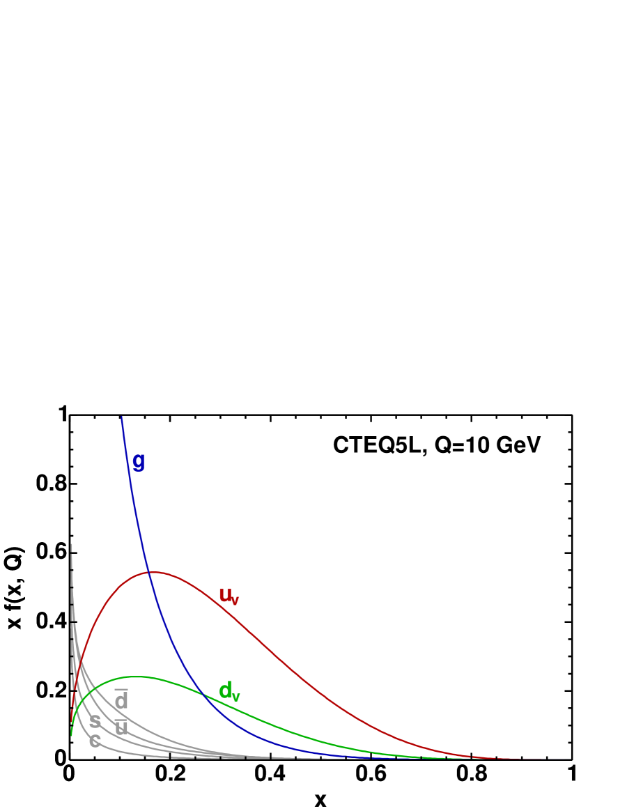
Figure C.1: Proton’s parton density functions.

The differential cross section for $12\to 34$ can be written as

$$d\sigma=\frac{\left(2\pi\right)^{4}}{2\hat{s}}\frac{d^{3}p_{3}}{\left(2\pi\right)^{3}2E_{3}}\frac{d^{3}p_{4}}{\left(2\pi\right)^{3}2E_{4}}\delta^{4}(p_{1}+p_{2}-p_{3}-p_{4})dx_{1}dx_{2}f_{1}(x_{1})f_{2}(x_{2})\sum_{spins}\left|\mathcal{M}\right|^{2}_{12\to 34}$$ (C.2)

where $\hat{s}$ is the parton center-of-mass energy squared, $p_{i}$ ($E_{i}$) is the momentum (energy) of the $i$th particle, $x_{1,2}$ are the fractions of the momenta of the incoming beam particles carried by the incoming partons, $f_{i}(x_{i})$ are the PDF’s with an implicit dependence on the energy scale of the interaction, and $\sum_{spins}\left|\mathcal{M}\right|^{2}_{12\to 34}$ is the matrix element squared for the process averaged over the spins and colors of the incoming particles and summed over the spins and colors of the outgoing particles.

First we consider the phase space. We perform the integral over the three-momentum of $p_{4}$, and reexpress the integral over the momentum of $p_{3}$ in terms of the magnitude of the three-momentum $p$ in the parton center-of-mass frame and the angle with respect to the beam $\theta$ and the azimuthal angle $\phi$. Then we make a transformation using $\hat{s}=x_{1}x_{2}s$ with $s$ the $p\bar{p}$ center-of-mass energy squared and we get $dx_{2}=d\hat{s}/(sx_{1})$. After some algebra, the differential cross section becomes

$$d\sigma=\frac{p}{32\pi^{2}\hat{s}^{5/2}}d\cos\theta d\phi d\hat{s}\frac{dx_{1}}{x_{1}}x_{1}f_{1}(x_{1})x_{2}f_{2}(x_{2})\sum_{spins}\left|\mathcal{M}\right|^{2}_{12\to 34}$$ (C.3)

The angular part can be uniformly generated with $0<\phi<2\pi$ and $-1<\cos\theta<1$. The momentum fraction $dx_{1}/x_{1}$ part can be transformed to $\ln x_{1}$ and then uniformly generated. For the distribution over $\hat{s}$, we impose a minimum value of $\hat{s}$. There are two types of distributions to be smoothed in order to converge faster for the Monte Carlo simulation. One type is a power law distribution $1/\hat{s}^{\alpha}$ with $\alpha>1$ which is the rise in the cross section due to the photon exchange at small center-of-mass energies. The other type is the Breit-Wigner resonance due to the $Z$ boson exchange with a mass $m$ and a width $\Gamma$,

$$\begin{array}[c]{lllll}\int_{\hat{s}/s}^{1}\frac{dx_{1}}{x_{1}}&\rho\equiv\ln x_{1}&\to&\int d\rho&\mbox{uniformly}\\ \int_{\hat{s}_{min}}^{s}\frac{d\hat{s}}{\hat{s}^{\alpha}}&\rho\equiv\hat{s}^{(1-\alpha)}&\to&\int d\rho&\mbox{uniformly}\\ \int_{\hat{s}_{min}}^{s}\frac{d\hat{s}}{\left(\hat{s}-m^{2}\right)^{2}+m^{2}\Gamma^{2}}&\rho\equiv\tan^{-1}\left(\frac{\hat{s}-m^{2}}{m\Gamma}\right)&\to&\int d\rho&\mbox{uniformly}\end{array}$$ (C.4)

Second we consider the matrix element which is the interesting part. With a non-constant matrix element, the distribution is expected to deviate from the pure phase space distribution. Further, compared with the distributions described by the SM, there are probably deviations in the distributions in real data due to some unknown matrix elements of new physics. The effects shown in cross section could be an enhancement or a suppression, a new resonance, changes in the angular distributions, a divergence or a cancellation by interference, etc. A good deal of particle physics consists of the measurements and the interpretations of such effects in cross section. For the SM process $q\bar{q}\to\gamma^{*}/Z\to\tau\tau$, we have

$$\sum_{spins}\left|\mathcal{M}\right|^{2}_{12\to 34}=\begin{array}[t]{l}(\hat{t}-m_{3}^{2})(\hat{t}-m_{4}^{2})(|g^{RL}|^{2}+|g^{LR}|^{2})\\ +(\hat{u}-m_{3}^{2})(\hat{u}-m_{4}^{2})(|g^{LL}|^{2}+|g^{RR}|^{2})\\ +2m_{3}m_{4}\mathcal{R}e\{g^{RL}g^{RR*}+g^{LR}g^{LL*}\}\end{array}$$ (C.5)

where $\hat{t}=(p_{1}-p_{3})^{2}$, $\hat{u}=(p_{1}-p_{4})^{2}$, $m_{3,4}$ are the masses of the outgoing tau particles. In the center-of-mass frame using $p_{cm}^{2}=\frac{1}{4\hat{s}}[\hat{s}-(m_{3}+m_{4})^{2}][\hat{s}-(m_{3}-m_{4})^{2}]$, the value of $\hat{t}$ can be expressed as $\hat{t}=m_{3}^{2}-\hat{s}^{1/2}(E_{3}-p_{cm}\cos\theta)$, and the value of $\hat{u}$ can be expressed as $\hat{u}=m_{4}^{2}-\hat{s}^{1/2}(E_{4}-p_{cm}\cos\theta)$. The couplings are defined to be

$$g^{ab}=\sum_{i=\gamma*/Z}\frac{g_{in}^{a}g_{out}^{b}}{(\hat{s}-m_{i}^{2})^{2}+m_{i}^{2}\Gamma_{i}^{2}}$$ (C.6)

where the sum runs over $\gamma^{*}/Z$ the intermediate gauge bosons with mass $0/m_{Z}$ and width $0/\Gamma_{Z}$, and $g_{in}^{L,R}$ is the coupling of the gauge boson to the incoming partons and $g_{out}^{L,R}$ is the coupling of the gauge boson to the outgoing tau particles. The couplings to the fermions in the SM are listed in Table 2.4.

To summarize, the major parts for generating an event include: (a) generating randomly the incoming partons and incorporating the PDF’s, (b) generating randomly the kinematic variables which describe the event in the phase space of the final particles, and (c) calculating the matrix element. Now we can put the parts together and get the weight for an event by multiplying all of the factors. The weight is in GeV^-2 and we need to convert to picobarn with a conversion constant $3.89379\times 10^{8}$ GeV² pb.

After generating a large sample of events, we can fill the weights of the events into a histogram, for example, a one-dimensional histogram of $\hat{s}$ which is the invariant mass of the tau pairs. The differential cross section versus the invariant mass of the tau pairs can be obtained by dividing the histogram by the number of events generated and the size of the bins. The result is shown in Fig. 2.4 in Section 2.3.

Chapter D Separation Angle under Boost

The calculable case is to boost the simplest phase space, i.e. a two-body decay, from the rest frame to the lab frame, as shown in Fig. D.1. The two final particles are back-to-back in the rest frame. The separation angle $\alpha$ of the two final particles in the lab frame can be parametrized as a function of $\theta^{*}$ the polar angle in the rest frame, which has an equal probability to be any value between $0^{o}$ and $90^{o}$, and the boost $\gamma$.

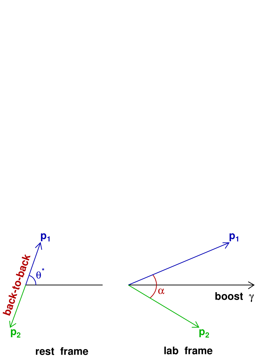
Figure D.1: Boost two-body decay from rest frame to lab frame.

Let us consider two massless final particles, e.g. two photons from a $\pi^{0}$ decay with a mass $m$, an energy $E$, and a boost $\gamma=E/m$. We boost the four-momentum of $p_{1}$ from the rest frame to the lab frame,

$$\left(\begin{array}[]{cccc}1&0&0&0\\ 0&1&0&0\\ 0&0&\gamma&\sqrt{\gamma^{2}-1}\\ 0&0&\sqrt{\gamma^{2}-1}&\gamma\end{array}\right)\left(\begin{array}[]{c}0\\ \frac{m}{2}\sin\theta^{*}\\ \frac{m}{2}\cos\theta^{*}\\ \frac{m}{2}\end{array}\right)=\left(\begin{array}[]{c}0\\ \frac{m}{2}\sin\theta^{*}\\ \frac{m}{2}(\gamma\cos\theta^{*}+\sqrt{\gamma^{2}-1})\\ \frac{m}{2}(\sqrt{\gamma^{2}-1}\cos\theta^{*}+\gamma)\\ \end{array}\right)$$ (D.1)

We denote the angle between $p_{1}$ in the lab frame and the direction of the boost as $\theta_{1}$. We have

$$\sin\theta_{1}=\frac{\sin\theta^{*}}{\sqrt{\sin^{2}\theta^{*}+(\gamma\cos\theta^{*}+\sqrt{\gamma^{2}-1})^{2}}}$$ (D.2)

We denote the angle between $p_{2}$ in the lab frame and the direction of the boost as $\theta_{2}$. By substituting $\theta^{*}$ with $\theta^{*}+\pi$, we have

$$\sin\theta_{2}=\frac{-\sin\theta^{*}}{\sqrt{\sin^{2}\theta^{*}+(-\gamma\cos\theta^{*}+\sqrt{\gamma^{2}-1})^{2}}}$$ (D.3)

Now we can calculate the separation angle $\alpha$,

$$\sin\alpha=\sin[\theta_{1}+(2\pi-\theta_{2})]=\frac{2\sin\theta^{*}\sqrt{\gamma^{2}-1}}{\sin^{2}\theta^{*}(\gamma^{2}-1)+1}$$ (D.4)

For $\theta^{*}$ not too small and $\gamma\gg 1$, we get an approximation for small $\alpha$,

$$\alpha\approx\frac{1}{\sin\theta^{*}}\times\frac{2}{\gamma}$$ (D.5)

For fixed $\theta^{*}$ (not too small) values, the functions are shown in Fig. D.3. For large boosts, the smearing by $\theta^{*}$ is small, thus the correlation between the separation angle and the boost (energy) is very strong.

Since $\theta^{*}$ has an equal probability to be any value between $0^{o}$ and $90^{o}$, the probability that the separation angle stays between the curve for $\theta^{*}=30^{o}$ and the curve for $\theta^{*}=90^{o}$ is three times larger than the probability that the separation angle stays between the curve for $\theta^{*}=10^{0}$ and the curve for $\theta^{*}=30^{o}$. The effect is very obvious. We use Monte Carlo simulation to check the same plot, as shown in Fig. D.3. It confirms that the simplest case of two-body decay is indeed calculable and the correlation between the separation angle and the boost (energy) is very strong.

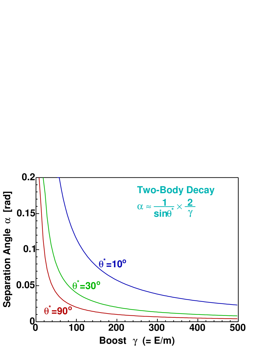
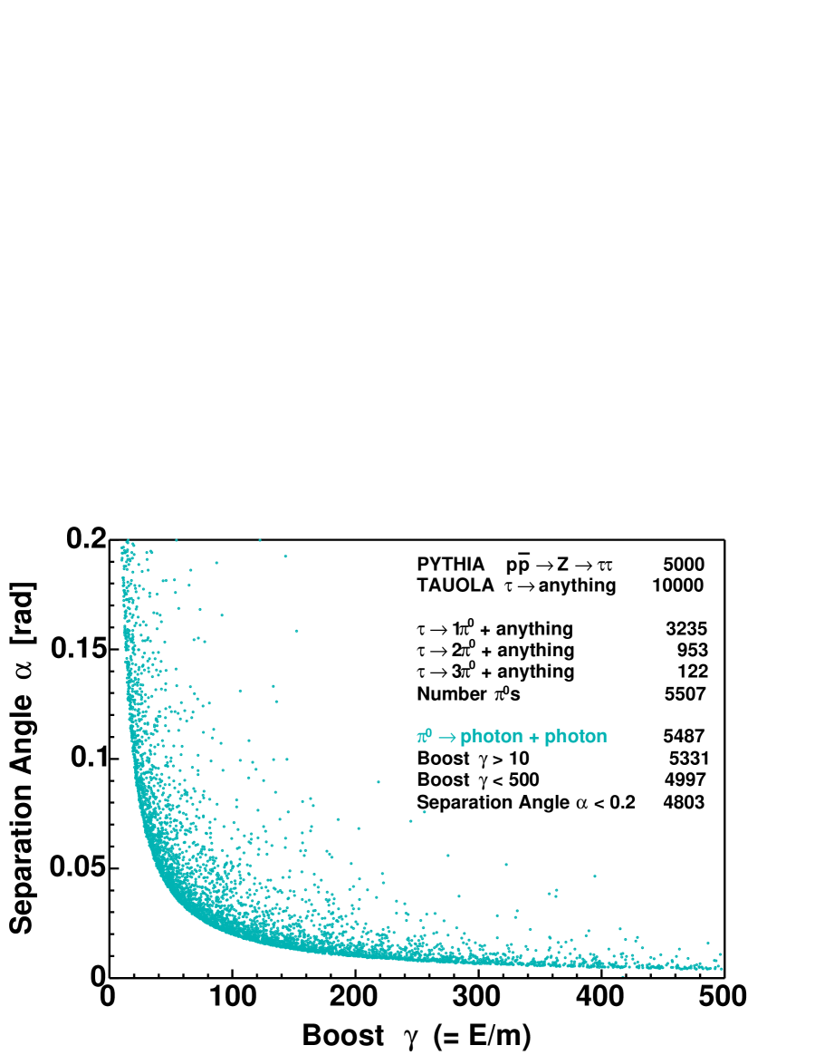
Figure D.2: Separation angle vs. boost, calculated in $\theta^{*}$ slices.

Figure D.3: Separation angle vs. boost, Monte Carlo distribution.

For the more complicated phase spaces such as those of tau’s hadronic decays, the calculation is very hard. But Eq. (D.5) is still a good hint. We need to use Monte Carlo simulation to get the distribution, which is shown in Fig. 5.4 in Section 5.2.2.

Curriculum Vita

Zongru Wan

1973	Born November 5 in Anhui, China.
1991	Graduated from Taihu High School, Anqing, Anhui, China.
1991-1995	Attended Beijing Institute of Technology, Beijing, China.
	Majored in Mechanical & Electrical Engineering.
1995	B.E. in Mechanical & Electrical Engineering.
	Beijing Institute of Technology, Beijing, China.
1995-1998	Research Staff, BES Collaboration
	at Institute of High Energy Physics, Beijing, China.
1999-2005	Graduate Studies in Physics
	at Rutgers, the State University of New Jersey, USA.
1999	Teaching Assistant, Department of Physics and Astronomy.
	Rutgers, the State University of New Jersey, USA.
1999-2005	Research Assistant, Department of Physics and Astronomy.
	Rutgers, the State University of New Jersey, USA.
2005	Ph.D. in Physics.
	Rutgers, the State University of New Jersey, USA.

Bibliography

- [1] J. Conway, L. Groer, V. Jacobs, C. Loomis, A.M. Walsh, and T. Watts, “Run 1B Charged Higgs Search”, CDF Note 3546 (1997).
- [2] S. Weinberg, Phys. Rev. Lett. 19, 1264 (1967); S. Weinberg, Phys. Rev. D5, 1412 (1972); A. Salam, in Nobel Symposium No. 8, ed. N. Svartholm (Almqvist and Wiksell, Stockholm, 1968); S.L. Glashow, Nucl. Phys. 22, 579 (1961); D.J. Gross and F. Wilczek, Phys. Rev. D8, 3633 (1973); D.J. Gross and F. Wilczek, Phys. Rev. D9, 980 (1974); H.D. Politzer, Phys. Rept. 14, 129 (1974).
- [3] S. Eidelman et al., Phys. Lett. B592, 1 (2004).
- [4] P.W. Higgs, Phys. Lett. 12, 132 (1964); P.W. Higgs, Phys. Rev. 145, 1156 (1966); F. Englert and R. Brout, Phys. Rev. Lett. 13, 321 (1964); G.S. Guralnik, C.R. Hagen and T.W.B. Kibble, Phys. Rev. Lett. 13, 585 (1964).
- [5] N. Cabibbo, Phys. Rev. Lett. 10, 531 (1963); M. Kobayashi and T. Maskawa, Prog. Theor. Phys. 49, 652 (1973).
- [6] M. Carena, A. Daleo, B.A. Dobrescu, and T.M.P. Tait, Phys. Rev. D70, 093009 (2004).
- [7] J. Wess and B. Zumino, Nucl. Phys. B70, 39 (1974).
- [8] H.P. Nilles, Phys. Rept. 110, 1 (1984); H.E. Haber and G.L. Kane, Phys. Rept. 117, 75 (1985); M. Carena and H.E. Haber, Prog. Part. Nucl. Phys. 50, 63 (2003).
- [9] V. Barger and R. Phillips, Collider Physics (Addison-Wesley, 1997).
- [10] M. Spira, hep-ph/9510347 (1995).
- [11] A. Djouadi, J. Kalinowski, and M. Spira, Comput. Phys. Commun. 108, 56 (1998).
- [12] D. Acosta et al., Phys. Rev. D71, 032001 (2005).
- [13] A. Sill et al., Nucl. Instrum. Meth. A447, 1 (2000).
- [14] T. Affolder et al., Nucl. Instrum. Meth. A526, 249 (2004).
- [15] L. Balka et al., Nucl. Instrum. Meth. A267, 272 (1988).
- [16] S. Bertolucci et al., Nucl. Instrum. Meth. A267, 301 (1988).
- [17] M.G. Albrow et al., Nucl. Instrum. Meth. A480, 524 (2002).
- [18] G. Ascoli et al., Nucl. Instrum. Meth. A268, 33 (1988).
- [19] R. Blair et al., FERMILAB-PUB-96-390-E (1996).
- [20] D. Acosta et al., Phys. Rev. Lett. 94, 091803 (2005).
- [21] T. Sjostrand et al., Comput. Phys. Commun. 135, 238 (2001).
- [22] H.L. Lai et al., Eur. Phys. J. C12, 375 (2000).
- [23] Z. Was, Nucl. Phys. Proc. Suppl. 98, 96 (2001).
- [24] GEANT3, CERN Program Library Long Writeup W5013 (1993).
- [25] A. Anastassov, J. Conway, D. Jang, A. Lath, F. Ratnikov, and Z. Wan, “Tau Reconstruction Efficiency and QCD Fake Rate for Run 2”, CDF Note 6308 (2003); A. Anastassov, “Non-isolated Reconstruction”, CDF Note 6688 (2003).
- [26] H.K. Gerberich, A.V. Kotwal, and C. Hays, “Cosmic Ray Tagging using COT Hit Timing”, CDF Note 6089 (2002).
- [27] S. Klimenko, J. Konigsberg, and T.M. Liss, FERMILAB-FN-0741 (2003).
- [28] R.G. Wagner, “Electron Identification for Run II: Algorithms”, CDF Note 5456 (2003).
- [29] M. Coca, E. Halkiadakis, and S. Lockwitz, “Central Electron Identification Efficiencies for the 200 pb-1 Run 2 Dataset”, CDF Note 6580 (2004).
- [30] E. Halkiadakis, C. Hays, M. Tecchio, and W. Yao, “A Conversion Removal Algorithm for the 2003 Winter Conferences”, CDF Note 6250 (2003).
- [31] T. Skwarnicki, DESY F31-86-02 (1986); D. Antreasyan et al., CB (Crystal Ball) Note 321 (1983).
- [32] J. Conway, R. Erbacher, R. Hughes, R. Marginean, R. Roser, E. Thomson, and B. Winer, “Measurement of the Cross Section Using Event Kinematics in Collisions at 1.96 TeV”, CDF Note 7288 (2005).
- [33] J. Bellinger et al., “A Guide to Muon Reconstruction for Run 2”, CDF Note 5870 (2002).
- [34] V. Martin and L. Cerrito, “Muon Cuts and Efficiencies for 4.11 Analyses”, CDF Note 6825 (2004).
- [35] A. Anastassov et al., Nucl. Instrum. Meth. A518, 609 (2004).
- [36] W. Badgett, H. Frisch, R.S. Denis, and T. Vaiciulis, “The Good Run List”, CDF Note 5613 (2001).
- [37] S. Baroiant et al., “Measurement of Electron Trigger Efficiencies for Level1 and Level2 8 GeV Triggers”, CDF Note 6257 (2003); S. Baroiant et al., “Measurement of Level 3 Trigger Efficiency for 8 GeV Inclusive Electron Trigger Using Conversions”, CDF Note 6324 (2003); S. Baroiant et al., “XFT Efficiency for the Isolated Track Leg of the Electron+Track Trigger”, CDF Note 6510 (2003); S. Baroiant et al., “Lepton+Track Triggers: Measurement of the Level 3 Trigger Efficiency for Taus”, CDF Note 6553 (2003); A. Anastassov, J. Conway, D. Jang, A. Lath, F. Ratnikov, and Z. Wan, “Muon Trigger Efficiencies for v4.11.1 Tau Data”, CDF Note 7429 (2005).
- [38] J. Conway, “Calculation of Cross Section Upper Limits Combining Channels Incorporating Correlated and Uncorrelated Systematic Uncertainties”, CDF Note 6428 (2005).
- [39] J. Field, Tests of the Standard Electroweak Model at LEP, Six Lectures given at EPFL Lausanne in April-June 1994 for the Troisième Cycle de Physique en Suisse Romande (1994).
- [40] E. Fermi, Nuovo Cim. 11, 1 (1934); E. Fermi, Z. Phys. 88, 161 (1934).
- [41] T.D. Lee and C.-N. Yang, Phys. Rev. 104, 254 (1956); C.S. Wu, E. Ambler, R.W. Hayward, D.D. Hoppes, and R.P. Hudson, Phys. Rev. 105, 1413 (1957); R.L. Garwin, L.M. Lederman, and M. Weinrich, Phys. Rev. 105, 1415 (1957).
- [42] R.P. Feynman and M. Gell-Mann, Phys. Rev. 109, 193 (1958); E.C.G. Sudarshan and R.E. Marshak, Phys. Rev. 109, 1860 (1958).
- [43] M. Gell-Mann, Phys. Lett. 8, 214 (1964); G. Zweig, CERN-TH-412 (1964), in Developments in the Quark Theory of Hadrons, ed. D.B. Lichtenberg and S.P. Rosen (Hadronic Press, 1986).
- [44] S.L. Glashow, Nucl. Phys. 22, 579 (1961).
- [45] G. Arnison et al., Phys. Lett. B122, 103 (1983); M. Banner et al., Phys. Lett. B122, 476 (1983); G. Arnison et al., Phys. Lett. B126, 398 (1983); M. Banner et al., Phys. Lett. B129, 130 (1983).
- [46] F.J. Hasert et al., Phys. Lett. B46, 138 (1973).
- [47] S.L. Glashow, J. Iliopoulos, and L. Maiani, Phys. Rev. D2, 1285 (1970).
- [48] J.J. Aubert et al., Phys. Rev. Lett. 33, 1404 (1974); J.E. Augustin et al., Phys. Rev. Lett. 33, 1406 (1974).
- [49] S.L. Adler, Phys. Rev. 177, 2426 (1969); J.S. Bell and R. Jackiw, Nuovo Cim. A60, 47 (1969).
- [50] S.L. Adler and W.A. Bardeen, Phys. Rev. 182, 1517 (1969); W.A. Bardeen, Phys. Rev. 184, 1848 (1969).
- [51] C. Quigg, Gauge Theories of the Strong, Weak, and Electromagnetic Interactions (Benjamin/Cummings, 1983); T.-P. Cheng and L.-F. Li, Gauge Theory of Elementary Particle Physics (Clarendon Press, Oxford, 1984); D.H. Perkins, Introduction to high energy physics (Cambridge University Press, New York, 1999); F. Halzen and A.D. Martin, Quarks and Leptons : an Introductory Course in Modern Particle Physics (Wiley, New York, 1984); A. Zee, Fearful Symmetry : the Search for Beauty in Modern Physics (Collier Books, New York, 1989); G.L. Kane, Modern Elementary Particle Physics, The Fundamental Particles and Forces? (Addison-Wesley, 1993); R.K. Ellis, W.J. Stirling and B.R. Webber, QCD and Collider Physics (Cambridge University Press, Cambridge, UK, 1996); A. Zee, Quantum Field Theory in a Nutshell (Princeton University Press, Princeton, NJ, 2003).
- [52] C.-N. Yang and R.L. Mills, Phys. Rev. 96, 191 (1954).
- [53] P. Richardson, “Tutorial on Writing Simple Event Generators and the Les Houches Accord”, http://www.ippp.dur.ac.uk/montecarlo/leshouches/tutorial (2003).