Nigel S. Lockyer
Supervisor of Dissertation

  Randall D. Kamien
Graduate Group Chairperson

To my grandfather

Acknowledgments

I would like to thank many people who taught me a tremendous amount and who helped me get through my time in graduate school. My thesis adviser, Prof. Nigel Lockyer, had provided me a full, solid training as a particle physicist. The experience of working on the electronics, the detector, and the particle identification tool, in addition to the physics analysis, is rare. I will always benefit from this in my following career life. Prof. Wei-Shu Hou at National Taiwan University motivated me to pursue research at High Energy Physics. Rick Tesarek, being my supervisor and mentor at Fermilab, taught me a lot about how to think critically about making measurements and at the same time not to dwell on the unimportant details. Joel Heinrich, though far away from Fermilab, was always supporting me at Penn. I could phone him any time to ask physics or statistics questions. I also gained interesting knowledge outside of physics from him. I would like to thank Dmitri Litvintsev, who helped us performing the measurement of the backgrounds and speeded up the progress of this analysis.

In the first two years of my graduate school, I learned a lot about the electronics from Mitch Newcomer, Rick Van Berg, Godwin Mayers and Chuck Alexander. I remembered the time asking Mitch questions late on Friday nights and the time working in Godwin’s lab with some homey chatting. Walter Kononenko helped me building the ASDQ test station and handled many details I tended to forget. After I moved to Fermilab, I spent months working on the detector with Dave Ambrose and Peter Wittich. We had fun going up and down in the lifts, fixing a broken fuse, torn cables and many other things. I obtained resources from Dave’s library and solved many puzzles. Peter always listened to my ranting and provided me some insight as a former Penn graduate student. Matthew Jones and Rolf Oldeman taught me a lot about B physics and asked important questions. The former and current Penn CDF graduate students, Chunhui Chen, Tianjie Gao, Denys Usynin, Andrew Kovalev, and Kristian Hahn, were good companions in the CDF trailers and DRL. I also would like to thank Prof. Joel Kroll and Prof. Brig Williams. They had kindly guided me when Nigel was very busy with the co-spokesperson responsibility.

I had a nice time taking shifts with the COT group: Aseet Mukherjee, Bob Wagner, Ken Schultz, Kevin Burkett, Robyn Madrak, Ayana Holloway, Carter Hall, Mike Kirby, JC Yun, Young-Kee Kim and Avi Yagil. Especially, Aseet let me understand the physics of drift chamber through many interesting debates and discussions. I also enjoyed the time outside of IB4 or CDF assembly hall with Robyn, Ayana, Carter and Kirby. Barry Wicklund and Prof. Marjorie Shapiro had watched very closely my work on $dE/dx$ and shared their rich experience in run I. Bill Orejudos helped writing the software for people to access $dE/dx$ easily. Stefano Giagu, Mauro Donega and Diego Tonelli performed the track-based $dE/dx$ calibration and made $dE/dx$ really usable. Mat Martin and Petar Maksimović patiently answered my questions about the fit to the $\Lambda_{b}\rightarrow\Lambda_{c}^{+}\pi^{-}$ mode. Guillelmo Gómez-Ceballos, Masa Tanaka, and Saverio DÁuria received my unexpected visits in the office often and helped me solving various technical problems.

My best friend in the US, Keng-hui Lin, carried a strong, optimistic attitude toward the life and that kept me going during the lowest point of my graduate student life. I wish I could do the same thing for her. I also would like to thank Jónatan Piedra and Alberto Belloni for enlarging my life. Most of all, finally, my family in Taiwan, father Shui-Beih Yu, mother Li-Yu Hsu, and sister Shin-Yun Yu, always cares about my health and is there for me and with me.

We present the first measurement of the ratio of branching fractions ${\cal B}(\Lambda_{b}\rightarrow\Lambda_{c}^{+}\mu^{-}\overline{\nu}_{\mu})/{\cal B}(\Lambda_{b}\rightarrow\Lambda_{c}^{+}\pi^{-})$ based on 171.5 $\mathrm{pb^{-1}}$ of $p\overline{p}$ collisions at $\sqrt{s}=1.96\rm~{}TeV$ taken with the CDF-II detector. In addition, we present measurements of ${\cal B}(\overline{B}^{0}\rightarrow D^{*+}\mu^{-}\overline{\nu}_{\mu})/{\cal B}(\overline{B}^{0}\rightarrow D^{*+}\pi^{-})$ and ${\cal B}(\overline{B}^{0}\rightarrow D^{+}\mu^{-}\overline{\nu}_{\mu})/{\cal B}(\overline{B}^{0}\rightarrow D^{+}\pi^{-})$, which serve as control samples to understand the data and Monte Carlo used for the $\Lambda_{b}$ analysis. We find the relative branching fractions of the control samples to be:

$$\frac{{\cal B}(\overline{B}^{0}\rightarrow D^{*+}\mu^{-}\overline{\nu}_{\mu})}{{\cal B}(\overline{B}^{0}\rightarrow D^{*+}\pi^{-})}=17.7\ \pm 2.3\ (stat)\pm 0.6\ (syst)\pm 0.4\ (BR)\pm 1.1\ (UBR),$$

and

$$\frac{{\cal B}(\overline{B}^{0}\rightarrow D^{+}\mu^{-}\overline{\nu}_{\mu})}{{\cal B}(\overline{B}^{0}\rightarrow D^{+}\pi^{-})}=9.8\ \pm 1.0\ (stat)\pm 0.6\ (syst)\pm 0.8\ (BR)\pm 0.9\ (UBR),$$

which are consistent with the ratios obtained by the Particle Data Group at the 0.7 and 1.1 $\sigma$ level, respectively. Finally, we obtain the relative $\Lambda_{b}$ branching fraction to be:

$$\frac{{\cal B}(\Lambda_{b}\rightarrow\Lambda_{c}^{+}\mu^{-}\overline{\nu}_{\mu})}{{\cal B}(\Lambda_{b}\rightarrow\Lambda_{c}^{+}\pi^{-})}=20.0\ \pm 3.0\ (stat)\pm 1.2\ (syst){+0.7\atop-2.1}\ (BR)\pm 0.5\ (UBR).$$

The uncertainties of the three relative branching fractions are from statistics, CDF internal systematics, external measured branching ratios and unmeasured branching ratios, respectively. We present a method to derive ${\cal B}(\Lambda_{b}\rightarrow\Lambda_{c}^{+}\pi^{-})$ using previous CDF measurements and obtain

$${\cal B}(\Lambda_{b}\rightarrow\Lambda_{c}^{+}\pi^{-})=\left(0.41\pm 0.19\ (stat\oplus syst){+0.06\atop-0.08}\ ({\it P_{T}})\right)\%,$$

where the last uncertainty is due to the measured $\Lambda_{b}$ $P_{T}$ spectrum. Combining ${\cal B}(\Lambda_{b}\rightarrow\Lambda_{c}^{+}\pi^{-})$ with our result, we determine the exclusive semileptonic branching fraction for the $\Lambda_{b}$;

$${\cal B}(\Lambda_{b}\rightarrow\Lambda_{c}^{+}\mu^{-}\overline{\nu}_{\mu})=\left(8.1\ \pm 1.2\ (stat){+1.1\atop-1.6}\ (syst)\pm 4.3\ ({\cal B}(\Lambda_{b}\rightarrow\Lambda_{c}^{+}\pi^{-}))\right)\%.$$

Chapter 1 Introduction

In this dissertation, we measure the properties of the lowest-mass beauty baryon, $\Lambda_{b}$. Baryons are the bound states of three quarks. Protons and neutrons, constituents of atomic nuclei, are the most common baryons. Other types of baryons can be produced and studied in the high-energy collider environment. Three-body dynamics makes baryons composed of low mass quarks difficult to study. On the other hand, baryons with one heavy quark simplify the theoretical treatment of baryon structure, since the heavy quark can be treated the same way as the nucleus in the atom. The $\Lambda_{b}$ is composed of $u$, $d$, and $b$ quarks, where the $b$ quark is much heavier than the other two. Although, it is accessible, little is known about $\Lambda_{b}$. In 1991, UA1 [1] reconstructed $9\pm 1$ $\Lambda_{b}\rightarrow J/\Psi\Lambda$ candidates. In 1996, ALEPH and DELPHI reconstructed the decay $\Lambda_{b}\rightarrow\Lambda_{c}^{+}\pi^{-}$ and found only 3-4 candidates [2, 3]. ALEPH measured a $\Lambda_{b}$ mass of $5614\pm 21$ ${\rm MeV}/{\rm c}^{2}$, while DELPHI measured $5668\pm 18$ ${\rm MeV}/{\rm c}^{2}$, about 2 $\sigma$ higher. Subsequently, CDF-I observed 20 $\Lambda_{b}\rightarrow J/\Psi\Lambda$ events [4], confirmed the existence of $\Lambda_{b}$ unambiguously and made a more precise measurement of $\Lambda_{b}$ mass, $5621\pm 5$ ${\rm MeV}/{\rm c}^{2}$. A recent CDF-II measurement by Korn [5] yields $5619.7\pm 1.7$ ${\rm MeV}/{\rm c}^{2}$, which will significantly improve the current world average, 5624$\pm$9 ${\rm MeV}/{\rm c}^{2}$, and resolve the discrepancy of ALEPH and DELPHI.

Several experiments have also measured the product of a fragmentation fraction and a branching ratio, such as: $f_{\Lambda_{b}}{\cal B}(\Lambda_{b}\rightarrow J/\Psi\Lambda)$ [4], and $f_{\Lambda_{b}}{\cal B}(\Lambda_{b}\rightarrow\Lambda_{c}^{+}\mu^{-}X)$  [6, 7]. However, branching ratios derived from measurements rely on the knowledge of the $\Lambda_{b}$ fragmentation fraction ($f_{\Lambda_{b}}$), which is defined as the probability for a $b$ quark to hadronize into $\Lambda_{b}$. Assuming that the $\Lambda_{b}$ dominates the production of the beauty baryons, i.e. $f_{\Lambda_{b}}\cong f_{\mathrm{baryon}}$, and applying the world average $f_{\mathrm{baryon}}$ compiled by the Particle Data Group (PDG) [8], we obtain the branching ratios:

$${\cal B}(\Lambda_{b}\rightarrow J/\Psi\Lambda)=(4.7\pm 2.8)\times 10^{-4},$$

and

$${\cal B}(\Lambda_{b}\rightarrow\Lambda_{c}^{+}\mu^{-}X)=(9.2\pm 2.1)\times 10^{-2}.$$

The uncertainties on the above branching ratios are large, about 60$\%$ and $20\%$. Several other decays, have been searched for, but either only 1 candidate was observed (eg: $\Lambda_{b}\rightarrow\Lambda_{c}^{+}a_{1}(1260)^{-}$) or no candidates were found (eg: $\Lambda_{b}\rightarrow pK^{-}$) and an upper limit was set. In addition to the mass and branching ratios, the $\Lambda_{b}$ lifetime is an important physics quantity. However, the world average lifetime ratio, $\tau(\Lambda_{b})/\tau(B^{0})$, is $0.797\pm 0.052$, in disagreement with the range of theoretical predictions: between 0.9 and 1.0 [9]. The properties listed above are all that is known about $\Lambda_{b}$ and its decays, which motivates us to measure the branching ratios of $\Lambda_{b}$.

Currently, the Fermilab Tevatron is the only facility which produces a large sample of $\Lambda_{b}$. The Heavy Quark Effective Theory (HQET) has been used to predict the mass, lifetime, and decay rates of the $\Lambda_{b}$. Studying $\Lambda_{b}$ at the Tevatron through various measurements allows us to test HQET in different aspects. We present a measurement of the relative branching fractions of $\Lambda_{b}\rightarrow\Lambda_{c}^{+}\mu^{-}\overline{\nu}_{\mu}$ to $\Lambda_{b}\rightarrow\Lambda_{c}^{+}\pi^{-}$. Figure 1.1 shows that these two decays have very similar Feynman diagrams: a $b$ quark decays into a $c$ quark via a virtual $W$ boson exchange, and $W$ decay into a muon and an anti-neutrino or an $\overline{u}$ and a $d$ quark. The advantage of measuring the ratio of branching fractions is that several systematic uncertainties cancel, such as those from the trigger and reconstruction efficiencies. To understand the $\Lambda_{b}$ measurement, we perform a similar analysis on the better understood $B_{d}$ decays: we measure ${\cal B}(\overline{B}^{0}\rightarrow D^{*+}\mu^{-}\overline{\nu}_{\mu})/{\cal B}(\overline{B}^{0}\rightarrow D^{*+}\pi^{-})$ and ${\cal B}(\overline{B}^{0}\rightarrow D^{+}\mu^{-}\overline{\nu}_{\mu})/{\cal B}(\overline{B}^{0}\rightarrow D^{+}\pi^{-})$.

Figure 1.1: Feynman diagram of $\Lambda_{b}\rightarrow\Lambda_{c}^{+}\mu^{-}\overline{\nu}_{\mu}$ (left) and $\Lambda_{b}\rightarrow\Lambda_{c}^{+}\pi^{-}$ (right) decays.

The analysis strategy is as follows: The number of signal events observed in the data ($N$) is the product of the number of produced $B$ hadrons ($N_{B}$), the branching ratio (${\cal B}$), the detector acceptance and reconstruction efficiency ($\epsilon$) obtained from a Monte Carlo (MC) program, i.e. $N=N_{B}\cdot{\cal B}\cdot\epsilon$. Therefore, the $\Lambda_{b}$ ($B^{0}$) relative branching fraction is the yield ratio divided by the efficiency ratio since the numbers of $B$ hadrons cancel. For the semileptonic mode, several backgrounds exhibit a similar signature to the real signal. We estimate the amount of these backgrounds ($N_{\mathrm{bg}}$) and subtract them from the observed yield in the data. The formula for extracting the relative branching ratio is then expressed as:

$$\frac{{\cal B}_{\mathrm{semi}}}{{\cal B}_{\mathrm{had}}}=(\frac{N_{\mathrm{inclusive\;semi}}-N_{\mathrm{bg}}}{N_{\mathrm{had}}})\times\frac{\epsilon_{\mathrm{had}}}{\epsilon_{\mathrm{semi}}}.$$

In this dissertation, we measure the following relative branching fractions:

$${\cal B}(\overline{B}^{0}\rightarrow D^{*+}\mu^{-}\overline{\nu}_{\mu})/{\cal B}(\overline{B}^{0}\rightarrow D^{*+}\pi^{-}), \mathrm{where}\;D^{*+}\rightarrow D^{0}\pi^{+},D^{0}\rightarrow K^{-}\pi^{+},$$

$${\cal B}(\overline{B}^{0}\rightarrow D^{+}\mu^{-}\overline{\nu}_{\mu})/{\cal B}(\overline{B}^{0}\rightarrow D^{+}\pi^{-}), \mathrm{where}\;D^{+}\rightarrow K^{-}\pi^{+}\pi^{+},$$

$${\cal B}(\Lambda_{b}\rightarrow\Lambda_{c}^{+}\mu^{-}\overline{\nu}_{\mu})/{\cal B}(\Lambda_{b}\rightarrow\Lambda_{c}^{+}\pi^{-}), \mathrm{where}\;\Lambda_{c}^{+}\rightarrow pK^{-}\pi^{+}.$$

In Chapter 2, a brief overview of the Standard Model and HQET is presented. A general description of the Tevatron, the CDF-II detector and trigger is found in Chapter 3. Chapter 4 details our data sample and event selection. Chapter 5 focuses on how the signal yields are extracted. The MC simulations for the acceptance and efficiency are described and compared with data in Chapter 6. Chapter 7 involves the estimate of the backgrounds present in the semileptonic signal. In Chapter 8, the systematic uncertainties are first discussed, then the results of the relative branching fractions are summarized. Through out the whole dissertation, the analyses of the $\Lambda_{b}$ and the $B^{0}$ control modes are presented in parallel. The charge conjugates of the $\Lambda_{b}$ and $B^{0}$ decays are also included in the reconstruction.

Chapter 2 Theoretical Background

This chapter first gives a brief overview of the fundamental particles and interactions in Section 2.1. Then a general idea of the Cabibbo-Kobayashi-Maskawa (CKM) matrix and the Heavy Quark Effective Theory (HQET) are discussed in Sections 2.2–2.3.

2.1 Fundamental Particles and Interactions

The “Standard Model” [10, 11] is the accepted theory that describes particles with no internal structure and their interactions with matter. In the Standard Model, the basic constituents of matter are six flavors of spin-1/2 quarks: the down-type quarks ($d$, $s$, $b$) and the up-type quarks ($u$, $c$, $t$), and six kinds of spin-1/2 leptons: the charged leptons, $e$, $\mu$ and $\tau$, and the neutrinos $\nu_{e}$, $\nu_{\mu}$, and $\nu_{\tau}$. The magnitude of the electron’s electric charge is denoted as “$e$”. The down-type quarks carry electric charge $-\frac{1}{3}e$ and the up-type quarks carry electric charge $+\frac{2}{3}e$. The charged leptons have electric charge -1$e$ while the neutrinos have zero electric charge. The masses of the quarks and leptons exhibit a hierarchy. The $u$, $d$ and $s$ quarks are much lighter ($<200$ ${\rm MeV}/{\rm c}^{2}$) than the $c$, $b$ and $t$ quarks ($\sim$ 1100, 4500 and 175000 ${\rm MeV}/{\rm c}^{2}$). This hierarchy is not understood. The three charged leptons also have progressively increasing masses: $\sim$ 0.51($e$), 106($\mu$), 1777($\tau$) ${\rm MeV}/{\rm c}^{2}$. For the neutrinos, currently, only upper limits exist for their masses. Separate neutrino types can undergo transitions into one another if at most one type of neutrino has zero mass. The current best estimates require three-flavor mixing to explain the full range of results from the solar neutrino [12, 13], and the atmospheric neutrino experiments  [14, 15, 16].

The Standard Model describes the following three types of interaction among quarks and leptons: electromagnetic, weak and strong interactions. The gravitational interaction is not described by the Standard Model. The gravitational force dominates in the large mass scale, such as a galaxy, but has little influence on the scale of quarks and leptons. Therefore, it is usually ignored in the fundamental particle interactions. The quarks and leptons interact via the exchange of the gauge bosons. The Lagrangian of each interaction is invariant under a transformation that corresponds to a symmetry group. The Standard Model is a theory based on the symmetry group $SU(3)\times SU(2)\times U(1)$. Both $SU(n)$ and $U(n)$ groups are Lie groups, i.e. any element in the group can be represented by $m$ fundamental elements or generators [17]:

$$E=\exp(\sum^{m}_{i}\theta_{i}F_{i}),$$ (2.1)

where $F_{i}$ is the $i^{\mathrm{th}}$ generator and $\theta_{i}$ is the “rotation” angle corresponding to each generator. Elements of the $SU(n)$ groups are represented by $n\times n$ unitary matrices, $U^{{\dagger}}U=1$, with det $U$ = +1 and have $n^{2}-1$ generators. The theory introduces $n^{2}-1$ gauge bosons, analogous to the rotation angle in Equation 2.1. They form a scalar product with the $n^{2}-1$ generators and make the Lagrangian invariant. The $U(1)$ group is a one dimensional unitary group with single generator, where the elements are specified by a continuous parameter, $\theta$, and expressed as $e^{i\theta}$.

The $U(1)$ group describes the electromagnetic interaction among quarks and the charged leptons, via the exchange of a massless spin-1 photon. The electromagnetic interaction binds the electrons and atomic nuclei together and forms atoms. The $SU(2)$ group describes the weak interaction experienced by all the fundamental particles, where the gauge bosons are massive spin-1 $W^{\pm}$ and $Z^{0}$. The masses of $W^{\pm}$ and $Z^{0}$ are about 80 and 91 ${\rm GeV}/{\rm c}^{2}$. A well known weak interaction process is the neutron $\beta$-decay: $n(udd)\rightarrow p(uud)e\overline{\nu}_{e}$. The right- and left-handed fundamental particles transform differently under $SU(2)$. The right-handed quarks and leptons do not couple to $W^{\pm}$ and are singlets under $SU(2)$. While the left-handed quarks and leptons are doublets under $SU(2)$ and classified into three generations:

$$L_{L} = \left(\begin{array}[c]{ccc}\left(\begin{array}[c]{c}\nu_{e}\\ e\end{array}\right)_{L},&\left(\begin{array}[c]{c}\nu_{\mu}\\ \mu\end{array}\right)_{L},&\left(\begin{array}[c]{c}\nu_{\tau}\\ \tau\end{array}\right)_{L}\end{array}\right),$$ (2.9)

$$Q_{L} = \left(\begin{array}[c]{ccc}\left(\begin{array}[c]{c}u\\ d\end{array}\right)_{L},&\left(\begin{array}[c]{c}c\\ s\end{array}\right)_{L},&\left(\begin{array}[c]{c}t\\ b\end{array}\right)_{L}\end{array}\right).$$ (2.17)

The weak interaction allows transitions between quarks of different flavors. The transitions within the same generation are more favored than those across the generations and the coupling strength is given by the CKM matrix (see Section 2.2). The coupling strength is the same for all leptons.

The $SU(3)$ group describes the strong color interaction among quarks, mediated via the exchange of eight massless spin-1 gluons. The quarks carry three possible “chromoelectric charges”: red, green and blue ($R,G,B$), which are analogous to the electric charge in the electromagnetic interaction. The eight gluons are associated with the color combinations:

$R\overline{B},R\overline{G},B\overline{R},B\overline{G},G\overline{R},G\overline{B},(R\overline{R}-G\overline{G})/\sqrt{2}$ and $(R\overline{R}+G\overline{G}-2B\overline{B})/\sqrt{6}$

The strong interaction binds the quarks together to form a colorless state, $q\overline{q}$ or $qqq$ ($R\overline{R}$ or $RGB$). The $q\overline{q}$ bound state is referred to as “meson” and the $qqq$ bound state is referred to as “baryon”. For example, a $\overline{b}d$ bound state is a $B^{0}$ meson and a $udb$ bound state is a beauty baryon, $\Lambda_{b}$. Both mesons and baryons are called “hadrons”. Just as the residual electric field outside of the neutral atoms causes them to combine into molecules, the residual color field outside of the protons and neutrons forms nuclei.

Each fundamental particle has an associated antiparticle, i.e. of which the electric charge, color charge and flavor are reversed, but the mass and the spin are the same. In addition, the Standard Model introduces a neutral spin-0 Higgs boson, $H^{0}$, to accommodate the masses of the gauge bosons, quarks and leptons. The Higgs boson has not been discovered, yet. The search for the Higgs boson remains an important goal of several running and future high energy experiments.

2.2 CKM Matrix

The strong interaction conserves the flavor of quarks, and only transitions of the same flavor quark will take place (eg: charmness conserved decay, $D^{*+}\rightarrow D^{+}\pi^{0}$), while the flavor-changing decays are allowed in the electroweak interaction (eg: beauty to charm decay, $\overline{B}^{0}\rightarrow D^{*+}\pi^{-}$). The Cabibbo - Kobayashi - Maskawa (CKM) matrix  [18, 19] in Equation 2.18 describes the coupling in the weak interaction between different flavors of quarks. For instance, $V_{cb}$ describes the electroweak coupling strength of the $b$ quarks to the $c$ quarks. The CKM matrix represents a unitary transformation from the flavor (mass) eigenstates to the weak interaction eigenstates.

$$V_{\mathrm{CKM}}\equiv\left(\begin{array}[c]{ccc}V_{ud}&V_{us}&V_{ub}\\ V_{cd}&V_{cs}&V_{cb}\\ V_{td}&V_{ts}&V_{tb}\end{array}\right).$$ (2.18)

A standard CKM matrix parametrization proposed by Chau,et al. [20, 21, 22, 23], which is similar to Kobayashi - Maskawa’s original parametrization [19], has four free parameters: three mixing angles between any two generations, $\theta_{12}$, $\theta_{23}$, $\theta_{13}$ and a phase, $\delta_{13}$;

$$V_{\mathrm{CKM}}= \left(\begin{array}[c]{ccc}c_{12}c_{13}&s_{12}c_{13}&s_{13}e^{-i\delta_{13}}\\ -s_{12}c_{23}-c_{12}s_{23}s_{13}e^{i\delta_{13}}&c_{12}c_{23}-s_{12}s_{23}s_{13}e^{i\delta_{13}}&s_{23}c_{13}\\ s_{12}s_{23}-c_{12}c_{23}s_{13}e^{i\delta_{13}}&-c_{12}s_{23}-s_{12}c_{23}s_{13}e^{i\delta_{13}}&c_{23}c_{13}\end{array}\right)$$ (2.22)

$$\cong \left(\begin{array}[c]{ccc}c_{12}&s_{12}&s_{13}e^{-i\delta_{13}}\\ -s_{12}c_{23}-c_{12}s_{23}s_{13}e^{i\delta_{13}}&c_{12}c_{23}-s_{12}s_{23}s_{13}e^{i\delta_{13}}&s_{23}\\ s_{12}s_{23}-c_{12}c_{23}s_{13}e^{i\delta_{13}}&-c_{12}s_{23}-s_{12}c_{23}s_{13}e^{i\delta_{13}}&c_{23}\end{array}\right)$$ (2.26)

with $c_{ij}=\cos\theta_{ij}$ and $s_{ij}=\sin\theta_{ij}$ where $i$, $j$ labels the generations. The matrix elements with simpler forms appearing in the first row and third column, have been measured directly in decay processes. $c_{13}$ is known to be very close to unity: $|c_{13}-1|\sim 10^{-6}$, and this gives an approximation in Equation 2.26. In the Standard Model, the complex phase, $\delta_{13}$, is the origin of the Charge-Parity (CP) violation in the weak interaction. We refer the reader to the Tevatron Run II B Physics Workshop Report  [9] for a more detailed description of the weak CP violation mechanisms.

Using the world average experimental results of the weak decays as the input, and assuming that only three generations exist, with the unitarity, a 90$\%$ confidence limit can be placed on the amplitude of the matrix elements (eg: $|V_{ud}|$);

$$\left(\begin{array}[c]{ccc}0.9739\sim 0.9751&0.221\sim 0.227&0.0029\sim 0.0045\\ 0.221\sim 0.227&0.9730\sim 0.9744&0.039\sim 0.044\\ 0.0048\sim 0.014&0.037\sim 0.043&0.9990\sim 0.9992\end{array}\right)$$ (2.27)

As seen in Equation 2.27, quark transitions within the same generation are favored over the transitions across generations. The latter are called “Cabibbo suppressed” decays. The goal of several analyses at CDF II, together with the experiments BELLE [24], BABAR [25] and KTeV [26], etc. , is to make precise measurements of many matrix elements. For example, a measurement of the $B^{0}-\overline{B}^{0}$ oscillation frequency can infer the CKM matrix element $V_{td}$. While $V_{ud}$ can be obtained by comparing the nuclear $\beta$-decay $n\rightarrow pe\overline{\nu}_{e}$ to muon decay and $V_{us}$ can be measured from the decay: $K\rightarrow\pi e\overline{\nu}_{e}$. By making measurements of all the CKM elements, we can determine whether the CKM matrix is unitary. If the matrix is not unitary, this would be a signature for additional physics not currently described by the Standard Model.

2.3 Heavy Quark Effective Theory

This dissertation presents a measurement of the $\Lambda_{b}$ relative decay rates. The transition amplitude (${\cal M}$) that describes the decay rate of a $B$ hadron into some final state $f$, can be derived by drawing all the possible Feynman diagrams at the quark level and summing up all the contributions. The underlying weak interaction is simple but the strong interaction that binds the quarks into hadrons introduces complications. When the quarks or gluons travel over a distance of $1/\Lambda_{\mathrm{QCD}}$ or longer, the coupling constant of the strong interaction ($\alpha_{s}$) diverges, so perturbation theory breaks down and the nonperturbative effect takes over. For the energy scale of our concern, $\Lambda_{\mathrm{QCD}}$ is around 200 ${\rm MeV}/{\rm c}^{2}$.

One theoretical tool, the Operator Product Expansion (OPE)  [27], separates the perturbative from nonperturbative physics and ${\cal M}$ becomes:

$${\cal M}=-\frac{4G_{F}}{\sqrt{2}}V_{\mathrm{CKM}}\sum_{j}C_{j}\langle f|O_{j}|B\rangle\left[1+{\cal O}(\frac{m_{b}^{2}}{M_{W}^{2}})\right],$$ (2.28)

where $j$ indicates the contribution from the $j^{\mathrm{th}}$ Feynman diagram, $G_{F}$ is the Fermi coupling constant, $V_{\mathrm{CKM}}$ is the CKM matrix element in Equation 2.18. The Wilson coefficients  [27], $C_{j}$, act as effective coupling constants and contain the physics at short distance. The Wilson coefficients can be calculated using perturbation theory and are model independent. The $\langle f|O_{j}|B\rangle$ is usually referred to as the hadronic matrix element, where $O_{j}$ is a local operator. The hadronic matrix elements contain the long distance physics and can only be evaluated using nonperturbative methods. Contributions from the higher order operators are suppressed by a power of $m_{b}^{2}/M_{W}^{2}$, where $m_{b}$ and $M_{W}$ are the masses of the $b$ quark and the $W$ boson. The Heavy Quark Effective Theory (HQET) significantly simplifies the form of the hadronic matrix element. This section gives a review of the HQET and shows how the $\Lambda_{b}$ decay rates may be derived using the HQET with other theoretical assumptions.

The HQET stems from the Standard Model and describes the hadrons containing a $b$ or $c$ quark. The concept of “heavy” is relative. In the HQET, the masses of the “heavy” $c$, $b$ and $t$ quarks are much larger than QCD energy scale, while the masses of the “light” $u$, $d$ and $s$ quarks are much smaller than $\Lambda_{\mathrm{QCD}}$. In the limit of $m_{c,b,t}\gg\Lambda_{QCD}$, a new type of symmetry, “spin-flavor heavy quark symmetry” arises. The momentum transfer between the heavy quark and the light quarks in the hadron system is of the order of $\Lambda_{\mathrm{QCD}}$. Or equivalently speaking, the typical size of a hadron system is of the order of $\Lambda_{QCD}^{-1}$. The change in the heavy quark velocity is then $\sim\Lambda_{QCD}/m_{Q}$, which vanishes when $m_{Q}$ is infinitely large. The velocity of the heavy quark is, therefore, almost unaffected by the strong interaction, i.e. the quark-quark interaction terms disappear in the Lagrangian. The only strong interaction of a static heavy quark is with gluons via choromoelectric charge. This quark-gluon interaction is spin-independent. Consequently, the light quark system knows nothing about the spin, mass and flavor of the “nucleus”, i.e. a $B$ hadron at rest is identical to a charm hadron at rest regardless of their spin orientations.

The “heavy quark symmetry” implies that we can relate properties of the beauty hadrons to those of the charm hadrons. For example, Aglietti [28] derived a formula to estimate the $\Lambda_{b}$ mass: $M_{\Lambda_{c}}-\frac{1}{4}(M_{D}+3M_{D^{*}})$ = $M_{\Lambda_{b}}-\frac{1}{4}(M_{B}+3M_{B^{*}})$, which gives $M_{\Lambda_{b}}\sim$ 5630 ${\rm MeV}/{\rm c}^{2}$, in good agreement with the world average, 5624$\pm$9 ${\rm MeV}/{\rm c}^{2}$. An analogy can be found in atomic systems, where the isotopes with different nuclei have nearly the same chemical properties. When performing a calculation of the $B$ or charm hadron mass, decay rate or lifetime, we could start from the limit of $m_{c,b,t}\gg\Lambda_{QCD}$. Then the correction terms are added in expansion of the power of $1/m_{Q}$, where $m_{Q}$ is the mass of the heavy quark. The $1/m_{Q}$ corrections take into account finite mass effects and are different for quarks of different masses. A more complete description of HQET may be found in Manohar[29], Godfrey [30] and Isgur [31].

The focus of this analysis, examining $\Lambda_{b}$ to $\Lambda_{c}$ baryon decay, is best suited to treatment using HQET since both the initial- and the final- state hadrons contain a heavy quark. In addition, the light quark system in a $\Lambda_{b}$ baryon is in a spin-0 state; the sub-leading corrections have a simpler form than those for the mesons [32]. This analysis concerns the relative branching fractions of $\Lambda_{b}\rightarrow\Lambda_{c}^{+}\mu^{-}\overline{\nu}_{\mu}$ to $\Lambda_{b}\rightarrow\Lambda_{c}^{+}\pi^{-}$, where the leading order Feynman diagrams are shown in Figure 1.1. Using the Soft Collinear Effective Theory (SCET), Leibovich, Ligeti, Stewart, and Wise [33] relate the decay rate of $\Lambda_{b}\rightarrow\Lambda_{c}^{+}\pi^{-}$ to $\Lambda_{b}\rightarrow\Lambda_{c}^{+}\mu^{-}\overline{\nu}_{\mu}$. The SCET assumes that in the $\Lambda_{b}\rightarrow\Lambda_{c}^{+}\pi^{-}$ decay, the pion mass can be neglected and $m_{b}-m_{c}\cong E_{\pi}\gg\Lambda_{\mathrm{QCD}}$. Therefore, the $\overline{u}d$ quark pair acquires large momentum, remains close together and acts as a color dipole (singlet). Within the $\Lambda_{b}$, the $b$ quark and the diquark ($ud$) form a color dipole since the $\Lambda_{b}$ is colorless; the same hold for the $c$ quark and the diquark within the $\Lambda_{c}$. The color dipole-dipole interaction is weaker than the color monopole-monopole interaction, which means the pion interacts weakly with the rest of the system. In the end, the $\Lambda_{b}\rightarrow\Lambda_{c}^{+}\pi^{-}$ decay factorizes into two subprocesses: the hadronization of the $\Lambda_{c}$ and, completely decoupled, the hadronization of the $\pi$. The hadronic matrix element is then expressed as $\langle\Lambda_{c}|\overline{c}\gamma^{\mu}(1-\gamma^{5})b|\Lambda_{b}\rangle\langle\pi|\overline{d}\gamma_{\mu}(1-\gamma^{5})u|0\rangle$. The first term is common to both hadronic and semileptonic decays and can be inferred from the differential decay rate of the semileptonic mode, $\frac{d\Gamma(\Lambda_{b}\rightarrow\Lambda_{c}^{+}\mu^{-}\overline{\nu}_{\mu})}{dw}$, at maximal recoil, where $w$ is the scalar product of the $\Lambda_{b}$ and $\Lambda_{c}$ four-velocities, $v$ and $v^{\prime}$:

$$w \equiv v\cdot v^{\prime}$$ (2.29)

$$= (m_{\Lambda_{b}}^{2}+m_{\Lambda_{c}}^{2}-q^{2})/(2m_{\Lambda_{b}}m_{\Lambda_{c}}).$$ (2.30)

Here $q^{2}$ is the four-momentum transfer in the decay. Maximal recoil refers to the kinematic configuration when the charged lepton and the neutrino momenta are parallel, or equivalently, when $q^{2}$ is at its minimum, $m_{l}^{2}$, which is approximately zero. At this configuration, semileptonic decay, $\Lambda_{b}\rightarrow\Lambda_{c}^{+}\mu^{-}\overline{\nu}_{\mu}$, has the same kinematics as the hadronic decay, $\Lambda_{b}\rightarrow\Lambda_{c}^{+}\pi^{-}$, since the $q^{2}$ of the hadronic decay is always $m_{\pi}^{2}$, which is neglected in the SCET, and $q^{2}\cong 0$. The $\frac{d\Gamma(\Lambda_{b}\rightarrow\Lambda_{c}^{+}\mu^{-}\overline{\nu}_{\mu})}{dw}$ can be constructed from six form factors, which are functions of $w$. The form factors can be considered as the Fourier transformation of the weak charge distribution and describe the interaction between the $b$ and the $c$ quarks. The second term of the hadronic matrix element is the pion decay constant, $f_{\pi}$. The value of $f_{\pi}$ is 131 MeV and was extracted from the decay width of $\pi^{-}\rightarrow\mu^{-}\overline{\nu}_{\mu}$.

In a more exact form, the $\Lambda_{b}\rightarrow\Lambda_{c}^{+}\pi^{-}$ decay rate is

$$\Gamma(\Lambda_{b}\rightarrow\Lambda_{c}^{+}\pi^{-})=\frac{3\pi^{2}(C_{1}+C_{2}/3)^{2}|V_{ud}|^{2}f_{\pi}^{2}}{m_{\Lambda_{b}}^{2}r_{\Lambda}}\left(\frac{d\Gamma(\Lambda_{b}\rightarrow\Lambda_{c}^{+}\mu^{-}\overline{\nu}_{\mu})}{dw}\right)_{w_{max}},$$ (2.31)

where $C_{1}$ and $C_{2}$ are the first two terms of the Wilson coefficients, the higher order terms are suppressed, and

$$r_{\Lambda} \equiv m_{\Lambda_{c}}/m_{\Lambda_{b}}.$$ (2.32)

The $w_{max}$ corresponds to $q^{2}=m_{l}^{2}\simeq m_{\pi}^{2}\simeq 0$. In the limit of $m_{Q}\gg\Lambda_{\mathrm{QCD}}$, the six form factors that describe the semileptonic differential decay rate are reduced to one universal function, the Isgur-Wise function ($\zeta(w)$) [31, 34], and

$$\frac{d\Gamma(\Lambda_{b}\rightarrow\Lambda_{c}^{+}\mu^{-}\overline{\nu}_{\mu})}{dw}=\frac{G_{F}^{2}m_{\Lambda_{b}}^{5}|V_{cb}|^{2}}{24\pi^{3}}r_{\Lambda}^{3}\sqrt{w^{2}-1}[6w+6wr_{\Lambda}^{2}-4r_{\Lambda}-8r_{\Lambda}w^{2}]\zeta^{2}(w).$$ (2.33)

Note that Equation 2.33 proposes an alternative way to measure $|V_{cb}|$ using $\Lambda_{b}\rightarrow\Lambda_{c}^{+}\mu^{-}\overline{\nu}_{\mu}$ decay.

Although HQET reduces the form factors to the Isgur-Wise function, it can not predict the functional form of $\zeta(w)$. One functional form easy for calculation was suggested by Isgur and Wise [31]:

$$\zeta(w)=e^{-\rho^{2}(w-1)},$$ (2.34)

where the slope $\rho^{2}$ has to be calculated using other theoretical assumptions. Assuming the number of colors ($N_{c}$) in the baryon is infinitely large, Jenkins, et al. [35] derived $\rho^{2}=1.3$. Using the QCD sum rules, Huang, et al. [36] calculated $\rho^{2}=1.35\pm 0.12$. A recent DELPHI measurement [37] gives $\rho^{2}=2.03\pm 0.46(stat){+0.72\atop-1.00}(syst)$, consistent with the numbers from Huang and Jenkins, et al.. Combining Equations 2.31–2.34 and the slope value from Jenkins, Leibovich, et al. predict ${\cal B}(\Lambda_{b}\rightarrow\Lambda_{c}^{+}\pi^{-})$ = 0.45$\%$ and ${\cal B}(\Lambda_{b}\rightarrow\Lambda_{c}^{+}\mu^{-}\overline{\nu}_{\mu})$ = 6.6$\%$. However, the correction to the large $N_{c}$ limit is of order $1/N_{c}$, which is 30$\%$ in the case of baryons ($N_{c}=3$). The uncertainty from the QCD sum rule is about 10$\%$.

To summarize, measuring the relative branching fractions of $\Lambda_{b}\rightarrow\Lambda_{c}^{+}\mu^{-}\overline{\nu}_{\mu}$ to $\Lambda_{b}\rightarrow\Lambda_{c}^{+}\pi^{-}$ allows us to obtain a ratio free from several experimental systematic uncertainties. With the external input of ${\cal B}(\Lambda_{b}\rightarrow\Lambda_{c}^{+}\pi^{-})$, we could infer the ${\cal B}(\Lambda_{b}\rightarrow\Lambda_{c}^{+}\mu^{-}\overline{\nu}_{\mu})$ and vice versa. Finally, the absolute branching ratios of $\Lambda_{b}\rightarrow\Lambda_{c}^{+}\pi^{-}$ and $\Lambda_{b}\rightarrow\Lambda_{c}^{+}\mu^{-}\overline{\nu}_{\mu}$ increase our knowledge of the $\Lambda_{b}$ baryon and test the validity of Equations 2.31 and 2.33 which are derived from the HQET and the SCET.

Chapter 3 The CDF-II Detector and Trigger

The Fermilab Tevatron is currently the highest energy accelerator in the world. Protons and anti-protons ($p\overline{p}$) are accelerated in its $\sim$ 6 km (4 mile) circumference to be brought into collision with a center of mass energy of approximately 1.96 TeV. The collisions take place at the center of two detectors: the Collider Detector at Fermilab (CDF-II) and D0-II. These two detectors are about 120^∘ away from each other on the ring as indicated in Figure 3.1. The “luminosity” is a measure of collision rate normalized by the collision cross section, in unit of 1/sec$\cdot$cm². The common dimension for the time integrated luminosity is “barn^-1”, which is 10²⁴/cm². During 1992–1995, the predecessors of CDF-II and D0-II, CDF-I and D0-I had collected data with a time-integrated luminosity of $\sim$110 $\mathrm{pb^{-1}}$ (inverse pico-barn) and published more than 100 papers. This analysis uses data collected by the CDF-II experiment.

Both the accelerator and the collider detectors underwent major upgrades between 1997 and 2001. The main goals of these upgrades were to increase the luminosity of the accelerator, and to collect data samples with an integrated luminosity of 2 $\mathrm{fb^{-1}}$ (inverse femto-barn) or more. The upgraded Tevatron accelerates 36 bunches of $p$ and $\overline{p}$, whereas the previous accelerator operated with only 6$\times$6. Consequently, the time between collisions (or beam crossings) has decreased from 3.5 $\mu$s to 396 ns for the current collider. The new collider configuration required extensive detector upgrades at CDF-II to accommodate the shorter bunch spacings. In Section 3.1, we give an overview of how the proton and anti-proton beams are accelerated to their final center of mass energy of 1.96 TeV, and collided. We then describe in Sections 3.2 –3.5 the components of the CDF-II detector, and trigger, which are used to measure the properties of the particles produced in the $p\overline{p}$ collisions.

3.1 $p\overline{p}$ acceleration and collisions

Figure 3.1: Layout of the Fermilab accelerator complex. The proton (solid arrow) is accelerated at the Cockcroft-Walton, Linac, Booster, Main Injector and finally at the Tevatron. The anti-proton (dashed arrow) from the anti-proton source is first accelerated at the Main Injector and then at the Tevatron.

In order to create the world’s most energetic particle beams, Fermilab uses a series of accelerators. The diagram in Figure 3.1 shows the paths taken by protons and anti-protons from initial acceleration to collision in the Tevatron. The first stage of acceleration is in the Cockcroft-Walton pre-accelerator [38] , where H^- ions are created from the ionization of the hydrogen gas and accelerated to a kinetic energy of 750 keV. The H^- ions enter a linear accelerator (Linac) [39], approximately 500 feet long, where they are accelerated to 400 MeV. The acceleration in the Linac is done by a series of “kicks” from Radio Frequency (RF) cavities. The oscillating electric field of the RF cavities groups the ions into bunches. Before entering the next stage, a carbon foil removes the electrons from the H^- ions at injection, leaving only the protons. The 400 MeV protons are then injected into the Booster, a 74.5 m-diameter circular synchrotron. The protons travel around the Booster about 20,000 times to a final energy of 8 GeV.

Protons are then extracted from the Booster into the Main Injector  [40], where the protons are accelerated from 8 GeV to 150 GeV before the injection into the Tevatron. The Main Injector also produces 120 GeV protons, where the protons collide with a nickel target, and produce a wide spectrum of secondary particles, including anti-protons. In the collisions, about 20 anti-protons are produced per one million protons. The anti-protons are collected, focused, and then stored in the Accumulator ring. Once a sufficient number of anti-protons are produced, they are sent to the Main Injector and accelerated to 150 GeV. Finally, both the protons and anti-protons are injected into the Tevatron. The Tevatron, the last stage of Fermilab’s accelerator chain, receives 150 GeV protons and anti-protons from the Main Injector and accelerates them to 980 GeV. The protons and anti-protons travel around the Tevatron in opposite directions. The beams are brought to collision at the center of the two detectors, CDF-II and D0-II.

We use the term “luminosity” to quantify the beam particle density and the crossing rate. The luminosity in units of cm^-2s^-1 can be expressed as:

$${\cal L}=\frac{fN_{B}N_{p}N_{\overline{p}}}{2\pi(\sigma_{p}^{2}+\sigma_{\overline{p}}^{2})}F\left(\frac{\sigma_{l}}{\beta^{*}}\right)$$ (3.1)

where $f$ is the revolution frequency, $N_{B}$ is the number of bunches, $N_{p/\overline{p}}$ are the number of protons/anti-protons per bunch, and $\sigma_{p/\overline{p}}$ are the RMS beam sizes at the interaction point. $F$ is a form factor which corrects for the bunch shape and depends on the ratio of $\sigma_{l}$, the bunch length, to $\beta^{*}$, the beta function, at the interaction point. The beta function is a measure of the beam width, and is proportional to the beam’s $x$ and $y$ extent in phase space. Figure 3.2 shows the peak luminosities for the stores used in this analysis. The collision products are recorded in the CDF-II and D0-II detectors.

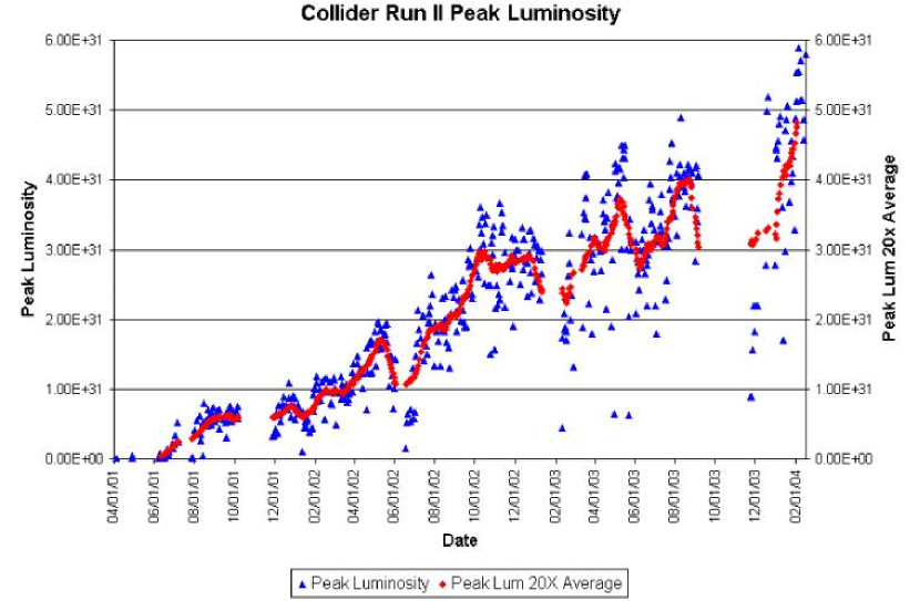
Figure 3.2: Peak luminosities for stores collided between April 2001 and February 2004. This analysis uses the data collected from February 2002 to September 2003.

3.2 The CDF-II Detector

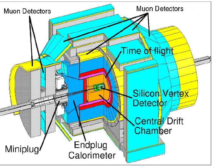
Figure 3.3: The CDF-II detector with quadrant cut to expose the different sub-detectors.

The Collider Detector at Fermilab (CDF) is a general purpose, azimuthally and forward-backward symmetric apparatus, designed to study $p\overline{p}$ collisions at the Tevatron. Figure 3.3 shows the detector and the different sub-systems in a solid cutaway view.

Standard Coordinates in CDF-II

Because of its barrel-like detector shape, CDF-II uses a cylindrical coordinate system ($r,\phi,z$) with the origin at the center of the detector. The $z$ axis is along the direction of the proton beam. The $r$ indicates the radial distance from the origin and $\phi$ is the azimuthal angle. The $r$-$\phi$ plane is called the transverse plane, as it is perpendicular to the beam line. The polar angle, $\theta$, is the angle relative to the $z$ axis. An alternative way of expressing $\theta$, pseudorapidity ($\eta$), is defined as:

$$\eta\equiv-\ln\tan(\theta/2).$$ (3.2)

The coverage of each CDF-II detector sub-system will be described using combinations of $\eta$, $r$, $\phi$ and $z$.

Overview

The CDF-II detector consists of five main detector systems: tracking, particle identification (for $e$, $K$, $p$ and $\pi$), calorimetry, muon identification and luminosity measurement.

The innermost system of the detector is the integrated tracking system: a silicon microstrip system and an open-cell wire drift chamber, the Central Outer Tracker (COT) that surrounds the silicon detector. The tracking system is designed to measure the momentum and the trajectory of charged particles. Reconstructed particle trajectories are referred to as “tracks”. Multiple-track reconstruction allows us to identify a vertex where either the $p\overline{p}$ interaction took place (primary vertex) or the decay of a long-lived particle took place (secondary or displaced vertex).

The silicon microstrip detector consists of three sub-detectors in a barrel geometry that extends from the radius of $r$= 1.35 cm to $r$= 28 cm and covers the track reconstruction in the range of $|\eta|<$ 2. Closest to the beam pipe is a single-sided, radiation tolerant silicon strip detector, Layer 00 (L00), with sensors at $r$=1.35 cm and $r$=1.62 cm. L00 is followed by five concentric layers of double-sided silicon sensors (SVX-II) from $r$=2.45 cm to 10.6 cm. The outermost silicon detector is the Intermediate Silicon Layers (ISL), from $r$=20 cm to $r$=28 cm. L00 only provides $r-\phi$ measurements, while the SVX-II and ISL provide both $r$-$\phi$ and $z$ measurements.

Surrounding the silicon detector is the COT, which covers the radius from 40 cm to 137 cm and $|\eta|<$ 1. Figure 3.5 and Figure 3.5 give a $r$-$z$ view of the CDF-II tracker and the silicon tracking system, respectively.

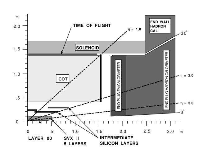
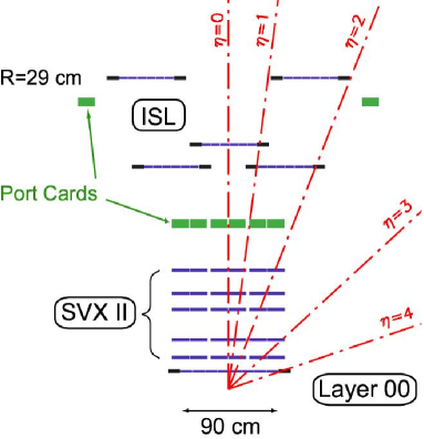
Figure 3.4: A diagram of the CDF-II tracker layout showing the different subdetector systems.

Figure 3.5: Coverage of the different silicon subdetector systems projected into the $r$-$z$ plane. The $r$ and $z$ axes have different scales.

Immediately outside the COT is the Time of Flight system (TOF), which consists of 216 scintillator bars, roughly 300 cm in length and with a cross-section of $4\times 4$ cm². The bars are arranged into a barrel around the COT outer cylinder. The TOF system is designed for the particle identification of charged particles with momentum below 2 $\rm GeV/c$. Both the tracking system and the TOF are contained in a superconducting solenoid, 1.5 m in radius, 4.8 m in length, that generates a 1.4 Tesla magnetic field parallel to the beam axis. The solenoid is surrounded by the electromagnetic and hadronic calorimeters, which measure the energy of particles that shower when interacting with matter. The coverage of the calorimeters is $|\eta|$ $<$ 3. The electromagnetic calorimeter is a lead/scintillator sampling device and measures the energy of the electrons and photons. The hadronic calorimeter is an iron/scintillator device and measures the energy of the hadrons, e.g.: pions.

The calorimeters are surrounded by the muon detector system. Muons interact with matter primarily through ionization. As a result, if a muon is created in the collision and has enough momentum, it will pass through the tracking system, TOF, the solenoid and the calorimeters with minimal interaction with the detector material. Muon detectors are, therefore, placed radially outside the calorimeters. The CDF-II detector has four muon systems covering different $\eta$ and $\phi$ regions: the Central Muon Detector (CMU), the Central Muon Upgrade Detector (CMP), the Central Muon Extension Detector (CMX), and the Intermediate Muon Detector (IMU). Figure 3.6 shows the coverage of each muon detector in the $\eta$-$\phi$ view.

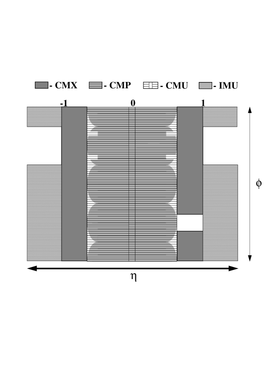
Figure 3.6: Locations of the CDF-II Muon System in the $\eta$-$\phi$ view.

At the extreme forward region of the CDF-II detector, 3.75 $<$ $|\eta|$ $<$ 4.75, two modules of Cherenkov Luminosity Counters (CLC) are placed pointing to the center of the interaction region to record the number of $p\overline{p}$ interactions. The number of particles recorded in the CLC modules is combined with an acceptance of the CLC ($A$) and the inelastic $p\overline{p}$ cross section ($\sigma_{in}$) to determine the instantaneous luminosity using the following equation:

$$L=\frac{\mu\cdot f_{BC}}{\sigma_{in}\cdot A}$$ (3.3)

where $L$ is the instantaneous luminosity, $f_{BC}$ is the rate of bunch crossings in the Tevatron and $\mu$ is the average recorded number of $p\overline{p}$ interactions per bunch crossing.

This analysis uses SVX-II, COT, CMU and the trigger, which will be described in detail in the following sections. More detailed information about each sub-detector and the trigger may be found in Bishai[41]. We refer the reader to Affolder and Hill[42, 43] for a full documentation about the ISL and L00, Acosta[44] about the TOF, Balka, Bertolucci and Kuhlmann [45, 46, 47] about the calorimeters, Artikov[48] about the CMP, the CMX and the IMU, and Acosta [49, 50] about the CLC.

3.3 Tracking Systems

3.3.1 Silicon Vertex Detectors II

Silicon tracking detectors are used to obtain precise position measurements of the path of a charged particle. They present some advantages over the gas filled drift chamber. The typical electron-hole creation energy of the silicon is about 3 eV, while the ionization energies are about 10–15 eV for the drift chamber gas (Argon or Ethane). The increased number of electrons gives better energy and position resolutions and signal to noise ratio. The fundamental component of the silicon detector is a reverse-biased p-n junction. The reverse-biased voltage increases the gap between the conduction band and the valence band across the p-n junction and reduces the current from the thermal excitation. By segmenting the p or n side of the junction into “strips” and reading out the charge deposition separately on every strip, we obtain sensitivity to the position of the charged particle. More information about the principles of silicon detector may be found in Knoll[51].

Table 3.1: Relevant parameters for the layout of the sensors of different SVX-II layers.

Property		Layer 0	Layer 1	Layer 2	Layer 3	Layer 4
number of $\phi$ strips		256	384	640	768	869
number of $Z$ strips		256	576	640	512	869
stereo angle	(∘)	90	90	+1.2	90	-1.2
$\phi$ strip pitch	($\mu$m)	60	62	60	60	65
$Z$ strip pitch	($\mu$m)	141	125.5	60	141	65
active width	(mm)	15.30	23.75	38.34	46.02	58.18
active length	(mm)	72.43	72.43	72.38	72.43	72.43

The CDF SVX-II is composed of double-sided silicon sensors. Each side measures either the $\phi$ or $z$ coordinates. The strips on the $\phi$ side run axially, while the strips on the $z$ side run either perpendicular to the axial strips, or are tilted by 1.2^∘. On the $\phi$ measurement side, 65 $\mu$m pitch strips of p-type silicon are implanted near the surface of a mild n-type (high purity) silicon bulk. On the $z$ measurement side, strips of n-type silicon are implanted on the same high purity bulk.

Four silicon sensors are assembled on a ladder. The readout electronics are mounted directly to the surface of the silicon sensor at each end of the ladder, as shown in Figure 3.8. The ladders are arranged in three, 29 cm long barrels in an approximately cylindrically symmetric configuration. The barrels are positioned end-to-end along the beam axis as shown in Figure 3.8, and segmented azimuthally into 12 wedges (30^∘ each). Each wedge contains 5 layers of silicon sensors. Table  3.1 gives the mechanical dimensions of SVX-II. The “impact parameter” is defined as the distance from the closest approach of the particle trajectory to the primary vertex. Without ISL and L00, SVX-II reaches a impact parameter resolution of $\sim$ 50 $\mu$m, which includes the 30 $\mu$m contribution from the transverse size of the beam line.

Figure 3.7: Prospective view of the $\phi$-side of a ladder for the SVX-II.

Figure 3.8: Isometric view of three SVX-II barrels.

3.3.2 Central Outer Tracker

The Central Outer Tracker (COT) is a cylindrical, open-cell drift chamber. The active volume of the COT begins from $r$=43.4 cm to $r$=132.3 cm and spans 310 cm in the $z$ direction. The COT contains 96 sense wire layers in the radial direction, which are grouped into eight superlayers, as shown in Figure 3.10. The maximum drift distance is approximately the same for all superlayers.

Each superlayer is divided in $\phi$ into “cells”. Figure 3.10 shows the transverse view of three COT cells. In each cell, 12 sense wires and 17 potential wires are sandwiched by two grounded field (cathode) sheets. The potential wires help shape the electric field near the sense wires. The distance between the wires and each field sheet is 0.88 cm. The sense wires alternate with the potential wires at a pitch of 0.3556 cm. Each end of the cell is closed with two potential wires, the first at the same pitch of 0.3556 cm, and the second at the pitch of 0.1778 cm. The wires are made of 40 $\mu$m of gold plated tungsten and the field sheets are made of 6.35 $\mu$m Mylar with vapor-deposited gold on each side. The entire COT contains 2,520 cells and 30,240 sense wires. The wires in superlayer 1, 3, 5 and 7 run along the $z$ direction (“axial”). The wires in the other superlayers are strung at a small angle ($2^{\circ}$) with respect to the $z$ direction (“stereo”).

The COT chamber is filled with an Argon-Ethane gas mixture and Isopropyl alcohol (49.5:49.5:1). The voltages on the sense wires are 2600-3000 volts and 1000-2000 volts on the potential wires. The field sheets are grounded. These voltages have been optimized using Garfield simulation software  [52] in order to achieve a gas gain of $2\cdot 10^{4}$ and minimize the drift field deviations from wire to wire. When a charged particle passes through, the gas is ionized. The applied electric field in the cell allows us to collect the electrons from the ionization and to track the passage of the charged particle. Electrons drift towards the sense wires with a velocity $\sim$ 50 $\mu$m/ns. Due to the magnetic field in which the COT is immersed, electrons drift at a Lorentz angle of $\sim 35^{\circ}$. Therefore, each cell is tilted by $35^{\circ}$ with respect to the radial direction to compensate for this effect. After the tilt, the electrons drift approximately perpendicular to the radial direction. The maximum electron drift time is approximately 177 ns, much shorter than the beam crossings of 396 ns. The electric potential in a cylindrical system grows logarithmically with decreasing radius. As a result, a limited avalanche via secondary ionization is initiated when the electron drifts close to the wire surface. This effect provides us a gain large enough to be read out by the electronics with high signal to noise.

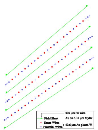
Figure 3.9: Layout of wire planes on a COT endplate.

Figure 3.10: Transverse view of three COT cells. Shown are cathode field sheets (solid lines), 12 sense wires (circles with cross) and 17 potential wires (marked by open circles) in each cell.

Signals on the sense wires are read out by the ASDQ (Amplifier, Shaper, Discriminator with charge encoding) chip, which was developed by Bokhari and Newcomer [53]. The ASDQ provides input protection, amplification, pulse shaping, baseline restoration, discrimination and charge measurement. The analog signal arrives at the ASDQ and the output is a digital pulse. The leading edge gives the arrival time information and the pulse width is related to the amount of charge collected by the wire. After calibrating the width variations due to the COT geometry, path length of the particle, gas gain difference for the 96 wires, the digital width is related to the ionization energy loss $dE/dx$, used for particle identification. A detailed description of the calibrations performed by the author and Donega, Giagu, Tonelli is found in Yu [54] and Donega [55].

The ASDQ pulse is then sent through $\sim 105$ cm of micro-coaxial cable, via repeater cards to Time to Digital Converter (TDC) boards in the collision hall. Hit times are later processed by pattern recognition (tracking) software to form helical tracks. The hit resolution of the COT is about 140 $\mu$m. The transverse momentum ($P_{T}$) resolution, $\sigma_{P_{T}}/P_{T}$ is about 0.15$\%\cdot P_{T}$. Table 3.2 lists the COT parameters. A full documentation about the COT may be found in Affolder [42].

Table 3.2: COT Parameters.

Parameter	Value
Gas	Ar/Et/Isopropyl(49.5:49.5:1)
Max. Drift distance	0.88 cm
Max. Drift Time	177 ns
Lorentz Angle	$\sim$ 31∘ (35 ∘cell tilt)
Drift Field	1.9 kV/cm
Radiation Lengths	1.7 $\%$
Total sense wires	30,240
Number of cells per SL	168,192,240,288,
	336,384,432,480
Stereo Angle	+2∘, 0∘, -2∘, 0∘
	+2∘, 0∘, -2∘, 0∘

3.3.3 Track Reconstruction

Definition of Track Parameters

Charged particles moving through a homogeneous solenoidal magnetic field in the $-z$ direction follow helical trajectories. To uniquely parameterize a helix in three dimensions, five parameters are needed: $C$, $\cot\theta$, $d_{0}$, $\phi_{0}$ and $z_{0}$. The projection of the helix is a circle on the $r$-$\phi$ plane. $C$ is the signed curvature of the circle, defined as $C\equiv\frac{1}{2Q\rho}$, where $\rho$ is the radius of the circle and the charge of the particle ($Q$) determines the sign of $C$. The positive charged tracks curve counterclockwise in the $r$-$\phi$ plane when looking into the $-z$ direction and the negative charged tracks bend clockwise. The transverse momentum, $P_{T}$, is related to $C$, the magnetic field ($B_{magnet}$), and charge of the particle:

$$P_{T}=Q\cdot\frac{1.49898\cdot 10^{-4}\cdot B_{magnet}}{C},$$ (3.4)

The $\theta$ is the angle between the $z$ axis and the momentum of the particle. Therefore, $\cot\theta$ is $P_{z}/P_{T}$, where $P_{z}$ is the $z$ component of the particle momentum. The last three parameters, $d_{0}$, $\phi_{0}$, and $z_{0}$, are the $r,\phi$ and $z$ cylindrical coordinates at the point of closest approach of the helix to the beam line. See Figure 3.12 for the definition of $d_{0}$ and $\phi_{0}$. $d_{0}$ is a signed variable;

$$d_{0}=Q\cdot(\sqrt{x_{0}^{2}+y_{0}^{2}}-\rho),$$ (3.5)

where $(x_{0},y_{0})$ is the center of the helix circle in the $r$-$\phi$ plane, Figure 3.12 illustrates the sign definition of $d_{0}$.

For decaying particles, we define the displacement $L_{xy}$,

$$L_{xy}=\vec{d}\cdot\hat{P_{T}}$$ (3.6)

where $\vec{d}$ is the displacement of the decay vertex in the transverse plane, and $\hat{P_{T}}$ is the unit vector in the direction of $\vec{P_{T}}$.

Figure 3.11: Definition of $d_{0}$ and $\phi_{0}$.

Figure 3.12: Tracks of particles with positive/negative charge and positive/negative impact parameters.

Pattern Recognition Algorithms

The track reconstruction begins using only the COT information. The first step is to look for a circular path in the axial superlayers of the COT. The algorithm looks for 4 or more hits in each axial superlayer to form a straight line, or “segments”. The hits on the segment are reconstructed using the time difference between when the ionization occurs, $t_{0}$ (the collision time plus the time of flight of the charged particle) and when the signal is picked up by the wire (the leading edge time of the digital pulse from the TDC). The global time offset, readout time of the wires and cables, electronic channel pedestals, charged-based time slewing and non-uniform drift velocities are corrected before using the time difference (or drift time) in the tracking.

Once segments are found, there are two approaches to track finding. One approach is to link together the segments which are consistent with lying tangent to a common circle. The other approach is to constrain its circular fit to the beamline, and then add hits which are consistent with this path. Once a circular path is found in the $r-\phi$ plane, segments and hits in the stereo superlayers are added depending on their proximity to the circular fit. This results in a three-dimensional track fit. Typically, if one algorithm fails to reconstruct a track, the other algorithm will not.

Once a track is reconstructed in the COT, it is extrapolated into the SVX-II. A three-dimensional “road” is formed around the extrapolated track, based on the estimated errors on the track parameters. Starting from the outermost layer, and working inward, silicon clusters found inside the road are added to the track. As a cluster is added, a new track fit is performed, which modifies the error matrix for the track parameters and produces a narrower road. In the first pass of this algorithm, $r-\phi$ clusters are added. In the second pass, stereo clusters are added to the track. If there is more than one track with different combinations of SVX hits associated with the same COT track, the track with maximum number of SVX hits is chosen.

The track reconstruction efficiency in the COT is $\sim 95\%$ for tracks which pass through all 8 superlayers ($P_{T}\geq 400~{}{\rm MeV}/{\rm c}$ ) and $\sim 98\%$ for tracks with $P_{T}$ $>$ 10 $\rm GeV/c$. The SVX track reconstruction efficiency with the COT tracks in the denominator is about 93$\%$ for the tracks with at least 3 SVX $r$-$\phi$ hits. A complete description of the COT and the SVX tracking is found in Hays[56].

3.4 Central Muon Detector

The Central Muon Detector (CMU) is embedded in the central hadron calorimeter wedges at $r$=347 cm as shown in Figure 3.13 and covers $\eta$ $<$ 0.6. The detector is segmented in $\phi$ into 12.6^∘ wedges, while the calorimeter is segmented into 15^∘ wedges. This leaves a 2.4^∘ gap between each wedge. In addition, there is a gap between the east and west chambers at $\eta$=0. The detector is further segmented in $\phi$ into three 4.2^∘ modules. There are 72 modules at the east and west ends of the detector, which gives 144 modules in total. Each module has 4 layers of 4 rectangular drift cells. The dimension of the drift cell is 6.35 cm (x) $\times$ 2.68 cm (y) $\times$ 226.1 cm (z). Each cell has a 50$\mu$m stainless steel sense wire in the center.

The first and the third layers have small offset in the $\phi$ direction from the second and the fourth layers, which also means: for each $\phi$ module, two sense wires from the alternating layers ( 1 and 3 or 2 and 4) lie on a radial line. The other two sense wires lie on a line with a 2 mm offset from the first two. The ambiguity as to which side of the sense wire (in $\phi$) a track passes is resolved by determining which two layers of sense wires are hit first. The sense wires of alternating $\phi$ cells in the same layer are connected together so to enable readout at only one end of the chamber. Signals from the sense wires are discriminated and passed on to the same type of TDCs as used by the COT. Short tracks reconstructed using the TDC and ADC information are referred to as “stubs”. The muon stubs are matched to the reconstructed tracks to form a muon candidate. A $\chi^{2}$ is computed using the distance between the track and the stubs, the difference in the direction of the track and the stub, and the covariance matrix of the track. Full documentation about the CMU is found in Ascoli[57]. Table 3.3 lists the parameters of the CMU, where the pion interaction lengths and the multiple scattering are computed at a reference angle of $\theta$ = 90^∘.

Figure 3.13: Location of the Central Muon Detector (CMU).

Table 3.3: Parameters of the CMU.

Parameter	Value
$\eta$ coverage	$\leq$ 0.6
Drift tube cross-section	2.68 $\times$ 6.35 cm
Drift tube length	226.1 cm
Max drift time	800 ns
Total drift tubes	2304
Pion interaction lengths	5.5
Min detectable muon $P_{T}$	1.4 $\rm GeV/c$
Multiple scattering resolution	12cm/p

3.5 Triggers

The triggering systems play an important role in the $p\overline{p}$ collider for two reasons. First, the collision rate is about 2.5 MHz, which is much higher than the rate at which data can be stored on tape, 50 Hz. Second, the total hadronic cross-section (including the elastic, inelastic, and diffractive processes) is about 75 mb and the $b\overline{b}$ cross-section is about 1000 times smaller, 0.1 mb. Extracting the most interesting physics events from the large number of events reduces the cost and time to reconstruct data.

The goal of the CDF-II triggering system is to be dead-time-less so that the system is quick enough to make a decision for every single bunch crossing before the next bunch crossing occurs. Each level of the trigger must reduce the background to a low enough level so that the rate to the next level is not saturated. Each level of the trigger is given an amount of time to make a decision about accepting or rejecting an event which depends on the complexity of the reconstruction. At the first level (Level 1), a trigger decision is made based only on a subset of the detector and quick pattern recognition or simple counting algorithms. The second level of the trigger (Level 2) does a limited event reconstruction. The third level of the trigger (Level 3) uses the full detector information to fully reconstruct events in a processor farm. The decision time for Level 1, 2 and 3 is about 5.5 $\mu s$, 20 $\mu s$ and 1 s, respectively. The event accept rate for Level 1, 2 and 3 is 40 kHz, 300 Hz and 50 Hz. The delay necessary to make a trigger decision is achieved by storing detector readout information in a storage pipeline, as shown in Figure 3.15.

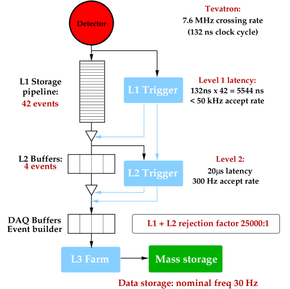
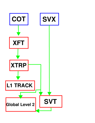
Figure 3.14: Diagram of the CDF-II trigger system.

Figure 3.15: Diagram of the two track trigger path at Level 1 and 2.

A trigger path is a well defined sequence of Level 1, Level 2 and Level 3 triggers. An event coming from one trigger path satisfies the trigger requirements at each level. A well defined trigger path eliminates volunteer events. A volunteer event is an event which passes a higher level trigger requirement but passes a lower level trigger from a different path. At CDF II, there are about 100 trigger paths. The trigger path used in this analysis is one of the SVT trigger paths, B$\_$CHARM Scenario A. Figure 3.15 shows a general diagram of the SVT trigger path.

The strategy of the SVT trigger path is as follows. At Level 1, the eXtremely Fast Tracker (XFT) measures the track $P_{T}$ and angle $\phi$. By cutting on $P_{T}$ and $\phi$, most of the inelastic background will be rejected. The Extrapolation Unit (XTRP) selects the XFT tracks above a certain $P_{T}$ threshold and sends signal to the Level 1 Track Trigger (Level 1 Track). The Level 1 Track Trigger counts the number of tracks from the XTRP, if more than 6 tracks are found, an automatic Level 1 accept is generated. Otherwise, depending on the trigger requirements, Level 1 Track Trigger accepts or rejects the event. If a Level-1 accept is received, the XFT track information is sent to the Level 2 Silicon Vertex Trigger (SVT). At Level 2, SVT uses the SVX-II information to obtain impact parameters of the tracks, $d_{0}$. Requiring non-zero impact parameters of tracks will require that they come from decays of long-lived particles: charmed and bottom hadrons. The requirements of each level of trigger will be described in detail in Section 3.5.4. The trigger components used in this trigger path, XFT, SVT, and Level 3, will be discussed in the following text. We refer the reader to the CDF Run II Technical Design Report [58] for a full descriptions of the trigger hardware.

3.5.1 The eXtremely Fast Tracker (XFT)

The Level 1 trigger decision of the “two track” trigger path is based on the information from the eXtremely Fast Tracker (XFT). This device is designed to measure the momentum of the charged particle using the hit information of the 4 COT axial layers. Instead of using the TDC information and a drift model to find a track segment as described in Section 3.3.3, the XFT uses a fast binary-like algorithm.

Each hit on the wire is classified as “prompt” if the drift time ranges from 0 to 66 ns and as “delayed” if the drift time ranges from 67 to 220 ns. Four neighboring COT cells are grouped together when searching for a segment in a given superlayer. A track segment in each axial superlayer is found by comparing the hit patterns to a list of pre-loaded patterns. The hit pattern varies depending on the combination of delayed and prompt hits, and the track angle through the cell or the track $P_{T}$. The algorithm allows two missed hits (2-miss) in each segment for the beginning period of the data used for this analysis and tightens the requirement to one missed hit (1-miss) since October, 2002. The data used in this analysis in the 2-miss period is about 26.4 $\mathrm{pb^{-1}}$, and 124.5 $\mathrm{pb^{-1}}$ for the 1-miss period.

Once a segment is found in a superlayer, it it marked as a “pixel”. XFT compares the pixels in all 4 layers to a list of pixel patterns in a $\Delta\phi=1.25^{\circ}$ window corresponding to a valid track with $P_{T}\geq$ 1.5 $\rm GeV/c$ ($\sim$ 2400 roads). The algorithm returns the best track. Figures 3.17–3.17 extracted from Thomson[59] show an example of the hit and the track pattern for a track with $P_{T}$ = 1.5 $\rm GeV/c$. Finally the XFT reports the track $P_{T}$ and $\phi_{6}$, the angle of the transverse momentum at the sixth superlayer of the COT, which is located 106 cm radially from the beamline.

The XFT efficiency is $\geq$ 96$\%$ for tracks which pass through all 4 axial layers. The momentum resolution, $\sigma_{P_{T}}/P_{T}$ is about 2$\%$ per $\rm GeV/c$. The angular resolution at the sixth superlayer, $\sigma_{\phi_{6}}$ is about 5 mR. More detailed information about XFT may be found in Thomson [59].

Figure 3.16: Close view of a track with $P_{T}$ = 1.5 $\rm GeV/c$ in a cell of the 4^th COT axial layer from Thomson[59]. A collection of the prompt hits (marked by open circles) and the delayed hits (marked by open diamonds) is an example of the XFT hit pattern.

Figure 3.17: Close view of a track with $P_{T}$ = 1.5 $\rm GeV/c$ traversing 4 COT axial layers from Thomson[59]. Several possible track patterns are displayed.

3.5.2 The Silicon Vertex Tracker (SVT)

At Level 2, the Silicon Vertex Tracker (SVT) combines the Level 1 track information, computes the track $d_{0}$, and improves the measurements of $P_{T}$ and $\phi_{0}$. The SVT is a new type of Level 2 trigger optimized for B physics . The heavy flavor particles, such as beauty and charm hadrons, decay at positions displaced from the primary vertices. Therefore, their daughter tracks tend to have larger impact parameters. The SVT cuts on the minimum track impact parameter so we are able to collect large sample rich in heavy flavor. The SVT also cuts on the maximum track impact parameter and removes background due to the long lived $K_{s}$, $\Lambda$ or the secondary tracks which come from the particles interaction with the beam pipes.

As mentioned in Section 3.3.1, the SVX-II is segmented into 12 wedges in $\phi$ and three mechanical barrels in $z$. The SVT makes use of this symmetry and does tracking separately for each wedge and barrel. The XFT track is extrapolated into the SVX-II, forming a “road”. Clusters of charge on the inner four $r-\phi$ layers of the given wedge have to be found inside this road. Since June 2003, the requirement is loosened to ask for hits from any four $r$-$\phi$ layers out the five SVXII layers. This period of data corresponds to about 1/3 of the total integrated luminosity used for this analysis. The SVT checks if one of the roads in the list of pre-loaded patterns is present in the data. The found roads are fed into a linearized fitter which returns the measurements of $p_{t},\phi_{0}$ and $d_{0}$ for the track. The Level 1 trigger conditions are confirmed with the improved measurements of $P_{T}$ and $\phi_{0}$. An event passes Level 2 selection if there is a track pair reconstructed in the SVT and additional requirements on the $d_{0}$, $L_{xy}$, and scalar sum $P_{T}$ of the track pair depending on the trigger path.

Figure 3.18 shows the SVT track impact parameter resolution for tracks with $P_{T}>2~{}\rm GeV/c$. The width of the Gaussian fit for the distribution in Figure 3.18 is 47 $\mu$m, which is a combination of the intrinsic SVT impact parameter resolution, and the transverse size of the beam line: $\sigma_{fit}=\sigma_{SVT}\oplus\sigma_{beam}$, where $\sigma_{beam}$ is about 30 $\mu$m. Therefore, the intrinsic SVT resolution is about 35 $\mu$m. Full documentation about SVT is found in Ashmanskas[60].

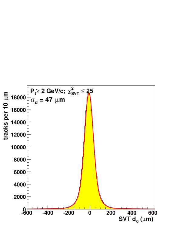
Figure 3.18: SVT impact parameter resolution.

3.5.3 Level 3 Trigger

The third level of the trigger system is implemented as a Personal Computer (PC) farm. The input rate of the Level 3 is roughly 300 Hz. With roughly 300 CPUs, and one event per CPU, this allocates approximately 1 second to do event reconstruction and reach a trigger decision.

Figure 3.19 shows the principle of the Level-3 farm. The detector readout from the Level 2 buffers is received via an Asynchronous Transfer Mode (ATM) switch and distributed to 16 “converter” node PC’s (CV). The main task of these nodes is to assemble all the pieces of the same event from the different sub-detector systems. The event is then passed via an Ethernet connection to a “processor” node (PR). Each processor node is a separate dual-processor PC. Each of the two CPU’s on the node process a single event at a time. The processor runs a “filter” executable which performs the near-final quality reconstruction. If the executable decides to accept an event, it is then passed to the “output” nodes of the farm (OU). These nodes send the event onward to the Consumer Server / Data Logger (CS/DL) system for storage first on disk, and later on tape. A full description of the Level 3 system is found in Gómez-Ceballos[61].

For the first two thirds of the data used in this analysis, the COT track reconstruction algorithms as described in Section 3.3.3 are performed at Level 3. The COT tracking returns $P_{T},z_{0},\phi_{0}$ and $\cot\theta$ and combines with the $d_{0}$ measurement from the SVT to create a further improved track. The Level 1 and Level 2 trigger conditions are confirmed at Level 3 using improved track measurements. For the last one third of the data, full SVX-II tracking is available, and the trigger conditions are repeated using a combined COT/SVX-II fit of the track helices.

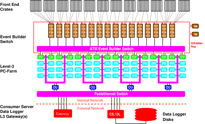
Figure 3.19: Event building and Level 3 operating principle: data from the front end crates is prepared by Scanner CPU’s (SCPU) and fed into the ATM switch. On the other side of the switch, converter nodes (CV) assemble events and pass them to processor nodes (PR). Accepted events are passed to output nodes (OU) which send them to the Consumer Server and Data Logging systems (CS/DL).

3.5.4 B$\_$CHARM Scenario A Trigger Path

The B$\_$CHARM Scenario A trigger path requires two tracks from the SVT and cuts on the $P_{T}$, the minimum and maximum $d_{0}$, the differences between the tracks’ parameters, such as $\Delta\phi_{0}$, $\Delta z_{0}$, and $L_{xy}$. $\Delta\phi_{0}$ is defined as the opening angle between the track pair in the $r$-$\phi$ plane. $\Delta z_{0}$ is the $z_{0}$ difference of the track pair. $L_{xy}$ is the distance of the intersection of two tracks with respect to the SVT beam line projected on the direction of the total momentum vector in the $r$-$\phi$ plane. The cuts at Level 1–3 triggers of B$\_$CHARM Scenario A trigger path are described below.

The trigger requirements are:

Level 1

• a pair of opposite charged XFT tracks

• each XFT track transverse momentum $P_{T}$ $>$ 2.04 $\rm GeV/c$

• scalar sum $P_{T}^{1}+P_{T}^{2}$ $>$ 5.5 $\rm GeV/c$

• $\Delta\phi_{0}$ $<$ 135 ^∘

Level 2

• a pair of opposite charged SVT tracks

• each SVT track satisfies:

  • SVT track fit $\chi^{2}<$ 25

  • $P_{T}$ $>$ 2 $\rm GeV/c$

  • SVT impact parameter: 120 $\mu$m $\leq d_{0}(SVT)\leq$ 1000 $\mu$m

• scalar sum $P_{T}^{1}+P_{T}^{2}$ $>$ 5.5 $\rm GeV/c$

• 2^∘ $<$ $\Delta\phi_{0}$ $<$ 90^∘

• $L_{xy}\geq$ 200 $\mu$m, this cut was added starting with run 150010 [62]

Level 3

The following cuts do not change for the whole period of taking data:

• each Level 3 track: $P_{T}$ $>$ 2 $\rm GeV/c$ and $|\eta|$ $<$ 1.2

• scalar sum $P_{T}^{1}+P_{T}^{2}$ $>$ 5.5 $\rm GeV/c$

• 2^∘ $<$ $\Delta\phi_{0}$ $<$ 90^∘

• $L_{xy}\geq$ 200 $\mu$m

• $\Delta z_{0}$ $<$ 5 cm

The following cuts are different for period I and II. All the number of time integrated luminosities are after the good run selection.

Period I: 9^th February 2002 to 19^th May 2003, Runs 138809–163113, $\sim$ 120 $\mathrm{pb^{-1}}$.

• Tracking algorithm at Level 3 uses only the COT hits and Level 3 tracks should be matched to Level 2 tracks found by the SVT

  • Track azimuthal angle difference: $\Delta(\phi_{0L3}-\phi_{0SVT})$ $<$ 0.015 radians

  • Curvature difference: $\Delta(C_{L3}-C_{SVT})$ $<$ 0.00015 cm^-1

• 120 $\mu$m $\leq d_{0}(L3)\leq$ 1000 $\mu$m, $d_{0}$ is calculated using SVT beamline

Period II: 19^th May 2003 to 6^th September 2003, Runs 163117–168889, $\sim$ 50 $\mathrm{pb^{-1}}$.

• Tracking algorithm at Level 3 uses both the SVX and COT hits

  • require at least 3 hits in different SVX layers

  • no attempt to match Level 3 tracks to SVT tracks

• 80 $\mu$m $\leq d_{0}(L3)\leq$ 1000 $\mu$m, $d_{0}$ is calculated using SVT beamline

Data derived from the above trigger path were written to the tape for subsequent reconstruction and physics analysis.

Chapter 4 Data Samples

Data used in this analysis are collected with the upgraded CDF detector from 9^th February 2002 to 6^th September 2003 and cover runs 138809 through 168889. This period corresponds to an integrated luminosity of $\sim$237 $\mathrm{pb^{-1}}$. In this chapter, we present details of how we arrive at our final data sample, optimize the cuts. We describe the data sample used for this analysis in Section 4.1. The cuts that are applied to obtain a clean signal with low background are explored in Section 4.2.

4.1 Data Sample

4.1.1 Overview

We wish to reconstruct the decays of the $B^{0}$ and the $\Lambda_{b}$. The $c\tau$ of the $B^{0}$ and $\Lambda_{b}$ are about 460 and 370 $\mu$m, respectively. The $c\tau$ of $D^{0}$, $D^{+}$, $D_{s}^{+}$ and $\Lambda_{c}^{+}$ are about 120, 150, 300 and 60 $\mu$m. Long lived $K_{s}$ and $\Lambda$ have much longer lifetimes, 2-8 cm. Therefore, a minimum requirement on the distance between the beamline and the secondary vertex (decay length) removes contamination of short-lived charm hadrons. The daughter particles from the $B$ decays also tend to have a larger impact parameter ($d_{0}$) than the tracks produced at the primary vertex, as illustrated in Figure 4.1, but smaller $d_{0}$ than the daughter particles of $K_{s}$ and $\Lambda$. Consequently, a minimum and a maximum cut on the track $d_{0}$ rejects the background from the primary tracks, $K_{s}$ and $\Lambda$, or secondary tracks from the particle interaction with the detector material. The newly developed SVT trigger cuts on the decay length and the track $d_{0}$. It is the best trigger for distinguishing $B$ decays from other physics processes. Among all the SVT trigger paths, we find B$\_$CHARM Scenario A most suitable for this analysis. Section 3.5.4 presents the definition of the B$\_$CHARM Scenario A trigger path. The goal of any measurement is to have the smallest possible uncertainty. By recording data from the same trigger, the systematic uncertainties common to both modes cancel. We therefore select all our data from the B$\_$CHARM Scenario A trigger path.

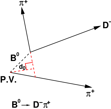
Figure 4.1: Example of a $B^{0}$ decay: $\pi^{+}$ from the $B^{0}$ decay has a larger impact parameter, $d_{0}$, than that of the track produced at the primary vertex, $\pi^{-}$.

The data from B$\_$CHARM Scenario A are processed with the Production executable, version 4.8.4, and compressed into the secondary datasets hbot0h and hbot1i. The total size of hbot0h and hbot1i is about 10 Terabytes (150M events), which is too big to be analyzed quickly multiple times. We apply loose selection cuts and reduce hbot0h, hbot1i to smaller, tertiary datasets. Section 4.1.2 discusses the data skimming. Then we optimize the analysis cuts using the tertiary datasets in Sections 4.2.

4.1.2 Data Skimming

Before skimming the data, we exclude the runs with an incorrect alignment table (152595–154012) in hbot0h. The alignment table contains the parameters for the positions of the COT and the SVX. The data during runs 152595–154012 are reprocessed with the correct alignment table and collected into hbot1i. We further require the following systems declared good by the CDF Data Quality Monitoring group: SVX, COT, CMU, Cherenkov Luminosity Counters (CLC) and the Level 1–3 triggers. We exclude the runs when SVX is off and when there are known high voltage or trigger problems in the COT, CMU or SVT. By making these requirements, the Monte Carlo program can better reproduce the response of these detectors (see Section 6.1). After making the good run selection, the integrated luminosity reduces from 237 $\mathrm{pb^{-1}}$ to 171.5 $\mathrm{pb^{-1}}$.

The skimming program starts by storing a set of offline reconstructed tracks which satisfy the quality requirements on: $P_{T}$, the number of COT hits in the axial and stereo layers, the number of SVX $r$-$\phi$ hits, and the impact parameter. Then, the tracks that are matched to those found by the SVT or to muon stubs (CdfMuon) in the CMU, are marked for further use. After saving the SVT and muon information, we begin our reconstruction by identifying the charm candidates: $D^{*+}$, $D^{+}$ and $\Lambda_{c}^{+}$.

We first cut on the raw mass of the charm candidates, where the raw mass is calculated using the track momentum at the point of closest approach to the beam line. We determine the charm (tertiary) vertex by performing a vertex fit with the CTVMFT package developed by Marriner [63]. CTVMFT determines the decay vertex by varying the track parameters of the daughter particles within their errors, so that a $\chi^{2}$ between the track trajectory and the points is minimized. We cut on the fitted charm mass and $\chi^{2}_{r-\phi}$, where “$\chi^{2}_{r-\phi}$” is the $\chi^{2}$ returned from the fit in the $r$-$\phi$ plane.

The charm candidate is then combined with an additional track to form the $B$ candidate. The additional track has a minimum $P_{T}$ requirement of 1.6 $\rm GeV/c$. Once we have a valid fourth track, we cut on the raw mass of the four tracks. The mass window varies depending on whether the fourth track is matched to a muon stub. We require that two of the four tracks from the reconstructed $B$-hadron candidate each matches an SVT track. We confirm the trigger by requiring the matched SVT tracks to pass the Scenario A cuts listed in Section 3.5.4. We then perform a four-track vertex fit. The four-track vertex fit includes a constraint that the tertiary vertex points to the secondary vertex in the $r$-$\phi$ plane. After the vertex fit, we cut on $P_{T}$ of the charm, the $\chi^{2}_{r-\phi}$, $P_{T}$ and fitted mass of the four tracks.

After applying the requirements discussed above for each signal mode, we reduce the secondary datasets, hbot0h and hbot1i, by a factor of 25 (from 10 to 0.4 Terabytes). The reduced datasets are then written to tape for further use. Detailed information about the skimming is found in the reference by the author et al. [64]. In Section 4.2, we present our analysis cut optimization with the reduced datasets.

4.2 Signal Optimization

From the reduced datasets we reconstruct our signals:

• $\overline{B}^{0}\rightarrow D^{*+}\pi^{-}$ and $\overline{B}\rightarrow D^{*+}\mu^{-}X$, where $D^{*+}\rightarrow D^{0}\pi^{+}$, $D^{0}\rightarrow K^{-}\pi^{+}$

• $\overline{B}^{0}\rightarrow D^{+}\pi^{-}$ and $\overline{B}\rightarrow D^{+}\mu^{-}X$, where $D^{+}\rightarrow K^{-}\pi^{+}\pi^{+}$

• $\Lambda_{b}\rightarrow\Lambda_{c}^{+}\pi^{-}$ and $\overline{B}\rightarrow\Lambda_{c}^{+}\mu^{-}X$, where $\Lambda_{c}^{+}\rightarrow pK^{-}\pi^{+}$

The reconstruction procedure is similar to that described in Section 4.1.2 and Yu [64]. The following cuts are studied more carefully and optimized :

• $\chi^{2}_{r-\phi}$ of $B$ and charm vertex fit

• $P_{T}$ of $B$ and charm candidates

• $c\tau$ of $B$ and charm candidates: $L_{xy}\times\frac{M}{P_{T}}$.

Our semileptonic signals are larger than the hadronic signals, and the statistical uncertainty of the relative branching fraction measurement is dominated by the uncertainty of the number of events in the hadronic signals. Therefore, we optimize the hadronic mode only and apply the optimized cuts to the semileptonic mode. The optimized quantity is the significance, $\frac{S}{\sqrt{S+B}}$, where “$S$” is the number of signal and “$B$” is the number of background events.

For our optimization, the amount of signal, “$S$” comes from a MC as described in Section 6.1. The reason for using MC signal is that the data signal is small and susceptible to statistical biases. We generate MC with about 20 times more events than the data and eliminate this problem. In order to scale the significance close to the true value measured from the data, we apply a normalization factor $f_{c}$ on the signal MC,

$$f_{c}=\frac{S_{\mathrm{data}}}{S_{\mathrm{MC}}},$$ (4.1)

where $S_{\mathrm{data}}$ and $S_{\mathrm{MC}}$ are the amount of the signal found in the data and MC after applying loose cuts, and

$$S=f_{c}\times S_{\mathrm{MC}}.$$ (4.2)

Note that even though “$S$”, after scaling, is the same as $S_{\mathrm{data}}$ now, the uncertainty on “$S$” is $f_{c}\times\sqrt{S_{\mathrm{MC}}}$, is much smaller than the uncertainty of $S_{\mathrm{data}}$, $\sqrt{S_{\mathrm{data}}}$. Figure 4.2 shows a comparison of the number of signal in the data and in the MC after applying the normalization factor.

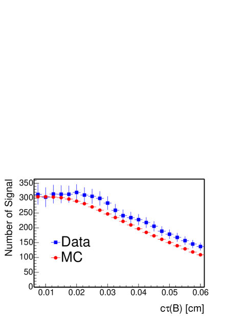
Figure 4.2: Signal optimization: number of signal in the MC and data as a function of the $c\tau(B)$ cut after applying the normalization factor for $\Lambda_{b}\rightarrow\Lambda_{c}^{+}\pi^{-}$.

We evaluate the background beneath the signal peak from the data. We first apply loose cuts on each mode to identify a clear $B^{0}$ or $\Lambda_{b}$ peak;

• $c\tau(B)$ $>$ 50 $\mu$m

• each track $P_{T}$  $>$ 0.5 $\rm GeV/c$

• $\pi$ from the $B$ hadron is CMU fiducial

• for $\overline{B}^{0}\rightarrow D^{*+}\pi^{-}$:

  • 1.833 $<$ $M_{K\pi}$ $<$ 1.893 ${\rm GeV}/{\rm c}^{2}$

  • 0.143 $<$ $M_{K\pi\pi}$ - $M_{K\pi}$ $<$ 0.148 ${\rm GeV}/{\rm c}^{2}$

• for $\overline{B}^{0}\rightarrow D^{+}\pi^{-}$: 1.8517 $<$ $M_{K\pi\pi}$ $<$ 1.8837 ${\rm GeV}/{\rm c}^{2}$

• for $\Lambda_{b}\rightarrow\Lambda_{c}^{+}\pi^{-}$: 2.269 $<$ $M_{pK\pi}$ $<$ 2.302 ${\rm GeV}/{\rm c}^{2}$

We require that both the muon and pion from the $B$ hadron point within CMU fiducial volume because we use the CMU only to identify the muons. CMU covers the region of pseudo-rapidity ($\eta$) less than 0.6. Making the same fiducial requirement for the hadronic mode allows the tracking efficiencies from both modes to cancel.

The backgrounds in the signal and in the upper mass regions are mainly combinatorial, and may be described by an exponential function, as we will see in Section 5.2. Therefore, we fit the upper mass region to an exponential function. Finally we extrapolate and integrate the exponential over the mass region of $\pm$ 3 $\sigma$ around the signal peak to obtain “$B$”. Figure 4.3 shows the $\Lambda_{b}$ mass distribution in the data and MC. The figure also shows the signal region we define and the upper mass region we fit to an exponential.

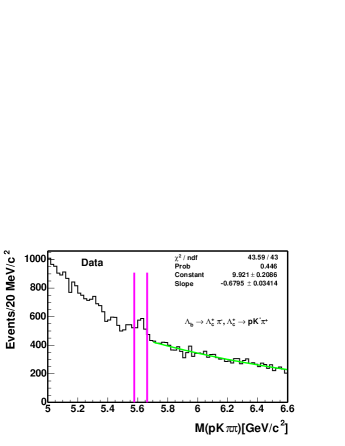
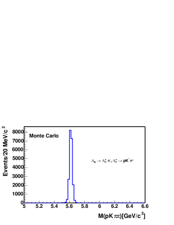
Figure 4.3: $\Lambda_{c}\pi$ invariant mass for data and MC. Left: data, the pink solid lines indicate the signal region. Right: MC.

The optimization follows an iterative procedure which passes through the data multiple times. In the first pass, cuts on each variable are scanned and optimization points are found. In the second pass, we apply the optimized cuts for all but the variable which is being re-optimized. We iterate this process several times until the optimization points become stable; usually twice is enough. Figures 4.4 shows $\frac{S}{\sqrt{S+B}}$, $\frac{S}{B}$ and $\frac{S}{S_{\mathrm{ref}}}$ from the optimization of $\Lambda_{b}\rightarrow\Lambda_{c}^{+}\pi^{-}$ mode, as a function of each cut variable, where $S_{\mathrm{ref}}$ is the number of signal events at the starting point. Tables 4.1– 4.2 list the final analysis cuts. Note that because the MC and the data $\chi^{2}_{r-\phi}$ do not agree well, as shown in Section 6.2, we choose to make a loose cut at the plateau region of the significance. The final analysis cuts for the $P_{T}$ of charm hadrons are tighter than the optimization points. The tighter cuts arise from the 4 $\rm GeV/c$ $P_{T}$ threshold applied to the $c$-quark in the MC sample for our semileptonic background study (see Section 7.4.2). This $P_{T}$ threshold makes the reconstruction of charm hadrons below 4 $\rm GeV/c$ inefficient. The MC sample is produced by the CDF $B$ group and it would take a prohibitive amount of CPU time to generate a new sample more suitable for our analysis. Therefore, we increase the $P_{T}$ cut of our charm hadrons to 5 $\rm GeV/c$. As the significance of the charm is a slowly varying curve, changing the cuts has little effect on the signal yield.

In addition to the cuts which are optimized above, we also require that the muon and pion from the $B$ hadron each matches an SVT track. Finally, for the semileptonic modes, we make cuts on the four track invariant mass (eg: $M(\Lambda_{c}\mu)$) to reduce the backgrounds from the other $B$ decays, see Section 7.2 for more details. The signal and sideband distribution of each optimized variable after $N-1$ cuts can be found in Yu [65]. The optimization yields a $S/B$ of 37.6 and 62.8 for the $\overline{B}^{0}\rightarrow D^{*+}\pi^{-}$ and $\overline{B}\rightarrow D^{*+}\mu^{-}X$ modes, 2.6 and 1.3 for the $\overline{B}^{0}\rightarrow D^{+}\pi^{-}$ and $\overline{B}\rightarrow D^{+}\mu^{-}X$ modes, 1.6 and 0.3 for the $\Lambda_{b}\rightarrow\Lambda_{c}^{+}\pi^{-}$ and $\overline{B}\rightarrow\Lambda_{c}^{+}\mu^{-}X$ modes. Figure 4.5 shows the charm+$\pi$ (left) and charm (right) mass spectra from the hadronic and inclusive semileptonic signals in the data after applying the optimized analysis cuts.

4.3 Summary

We have reconstructed our signals in the data collected from the trigger path B$\_$CHARM Scenario A. We have optimized our analysis cuts. In the next chapter, we will present the fit to the charm and $B$ hadron mass spectra to obtain the number of signal events.

Table 4.1: Final analysis cuts shared by all the modes.

All
$P_{T}$ for all tracks	$>$ 0.5 $\rm GeV/c$
$\pi_{B}$ and $\mu_{B}$ $P_{T}$	$>$ 2.0 $\rm GeV/c$
$P_{T}$ of 4 tracks	$>$ 6.0 $\rm GeV/c$
$P_{T}$ of charm hadron	$>$ 5.0 $\rm GeV/c$
$\mu_{B}$ CMU $\chi^{2}_{x}$	$<$ 9
every track exits at COT layer 95
$\pi_{B}$ and $\mu_{B}$ matched to SVT tracks and CMU fiducial

Table 4.2: Final analysis cuts for each mode.

$\overline{B}\rightarrow D^{*+}X$
$D^{0}$ VertexFit $\chi^{2}_{r-\phi}$	$<$ 16
4 track VertexFit $\chi^{2}_{r-\phi}$	$<$ 17
$c\tau$($D^{0}$ $\rightarrow$ $B$)	$>$ -70 $\mu$m
$c\tau$($B$ $\rightarrow$ beamspot)	$>$ 200 $\mu$m
1.833 $<$ $M_{K\pi}$ $<$ 1.893 ${\rm GeV}/{\rm c}^{2}$
3.0$<$ $M_{K\pi\pi\mu}$ $<$5.3 ${\rm GeV}/{\rm c}^{2}$ for $\overline{B}\rightarrow D^{*+}\mu^{-}X$
0.143$<\Delta m<$0.148 ${\rm GeV}/{\rm c}^{2}$ for $\overline{B}^{0}\rightarrow D^{*+}\pi^{-}$
$\overline{B}\rightarrow D^{+}X$
$D^{+}$ VertexFit $\chi^{2}_{r-\phi}$	$<$ 14
4 track VertexFit $\chi^{2}_{r-\phi}$	$<$ 15
$c\tau$($D^{+}$ $\rightarrow$ $B$)	$>$ -30 $\mu$m
$c\tau$($B$ $\rightarrow$ beamspot)	$>$ 200 $\mu$m
3.0$<$ $M_{K\pi\pi\mu}$ $<$5.3 ${\rm GeV}/{\rm c}^{2}$  for $\overline{B}\rightarrow D^{+}\mu^{-}X$
1.8517 $<$ $M_{K\pi\pi}$ $<$ 1.8837 ${\rm GeV}/{\rm c}^{2}$ for $\overline{B}^{0}\rightarrow D^{+}\pi^{-}$
$\Lambda_{b}\rightarrow\Lambda_{c}^{+}X$
$P_{T}$ of proton	$>$ 2 $\rm GeV/c$
$\Lambda_{c}^{+}$ VertexFit $\chi^{2}_{r-\phi}$	$<$ 14
4 track VertexFit $\chi^{2}_{r-\phi}$	$<$ 15
$c\tau$($\Lambda_{c}^{+}$ $\rightarrow$ $\Lambda_{b}$)	$>$ -70 $\mu$m
$c\tau$($\Lambda_{b}$$\rightarrow$ beamspot)	$>$ 250 $\mu$m
3.7$<$ $M_{pK\pi\mu}$ $<$5.64 ${\rm GeV}/{\rm c}^{2}$ for $\overline{B}\rightarrow\Lambda_{c}^{+}\mu^{-}X$
2.269$<$ $M_{pK\pi}$ $<$2.302 ${\rm GeV}/{\rm c}^{2}$  for $\Lambda_{b}\rightarrow\Lambda_{c}^{+}\pi^{-}$

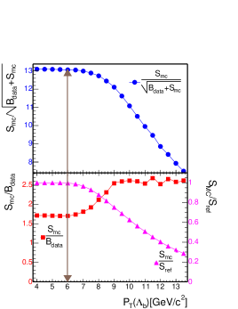
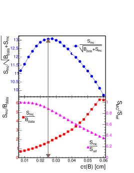
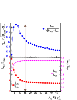
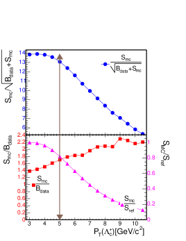
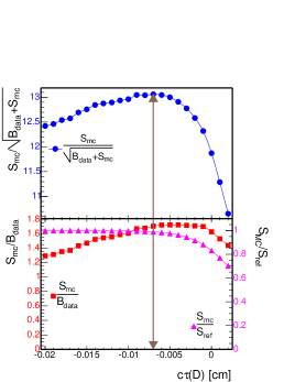
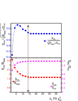
Figure 4.4: Significance ($\frac{S}{\sqrt{S+B}}$) marked by circles, signal/background ($\frac{S}{B}$) marked by squares and signal/reference ($\frac{S}{S_{\mathrm{ref}}}$) marked by triangles for cuts used in $\Lambda_{b}\rightarrow\Lambda_{c}^{+}X$ analysis.

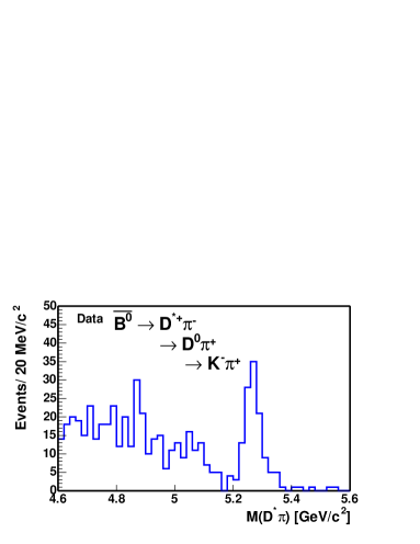
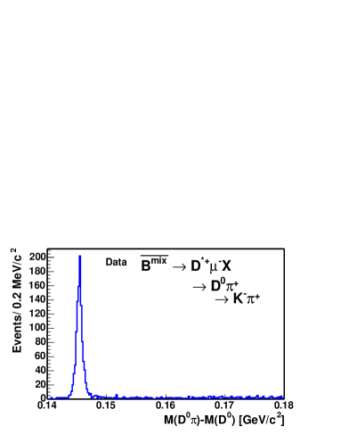
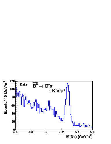
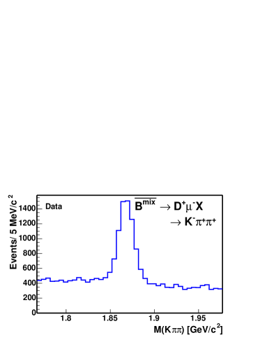
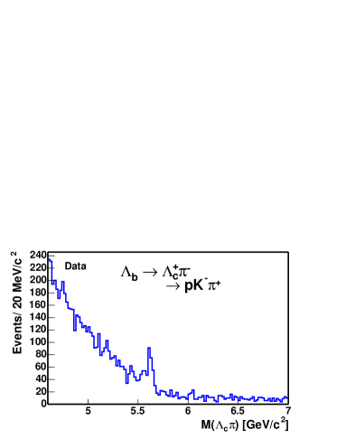
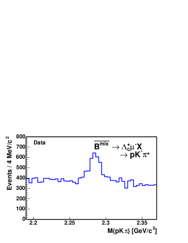
Figure 4.5: charm+$\pi$ and charm mass spectra from our signals after all cuts. From the top left to the bottom right are: $M_{D^{*}\pi}$, $M_{D^{0}\pi}-M_{D^{0}}$, $M_{D\pi}$, $M_{K\pi\pi}$, $M_{\Lambda_{c}}\pi$ and $M_{pK\pi}$.

Chapter 5 Signal Yield in the Data

In this chapter, we explain how the signal yield in the data is extracted. Ideally, if we were capable of fully reconstructing $B$ hadrons in both hadronic and semileptonic modes, we would use the $B$ hadron mass distribution to obtain the number of signal events (yield). However, a neutrino is missing in the semileptonic decay and the invariant mass of “charm+$\mu$” is a broad spectrum with a shape which is poorly distinguished from the backgrounds. Therefore, a proper variable to use for the semileptonic mode is the mass of the charm hadron. We extract the yield by fitting the charm+$\pi$ (or charm) mass spectra in Figure 4.5 to a function which describes both the signal and the background. We integrate the signal function to obtain the yield. The signal function for all modes is a Gaussian or double-Gaussians. The background function varies with the decay mode.

All our fits use an unbinned, extended likelihood technique. The general extended likelihood function ($\cal L$) is expressed as:

$$\log{\cal L}=\sum_{i}\log\{N_{\mathrm{sig}}\cdot{\cal S}(m_{i})+N_{\mathrm{bg}}{\cdot B}(m_{i})\}-N_{\mathrm{sig}}-N_{\mathrm{bg}}+\log{\cal C},$$ (5.1)

where $i$ represents $i^{th}$ event, $m$ represents the reconstructed charm+$\pi$ (charm) mass. The amounts of signal and background are denoted as $N_{\mathrm{sig}}$ and $N_{\mathrm{bg}}$, respectively, while ${\cal S}(m)$ (${\cal B}(m)$) are the functions which describe the signal (background) mass spectrum. The last term in Equation 5.1, ${\cal C}$, is a Gaussian constraint on one fit parameter, $x$:

$${\cal C}={\cal G}(x,\mu,\sigma)={1\over\sqrt{2\pi}\sigma}e^{-{1\over 2}({(x-\mu)\over\sigma})^{2}},$$ (5.2)

where we constrain the variable $x$ around the mean $\mu$. The difference of $x$ and $\mu$ follows a Gaussian distribution with an uncertainty $\sigma$. The unbinned likelihood fitter calls the ${\tt MINUIT}$ package developed by James et al. [66]. ${\tt MINUIT}$ varies the fit parameters to minimizes $-2\cdot\log{\cal L}$ .

The performance of the fitter was checked on 1000 toy MC samples similar to the data distribution. We plot the pull distribution for each parameter, i.e. $(x-x_{0})/\sigma_{x}$, where $x$ is the fit value, $x_{0}$ is the generated (input) value, and $\sigma_{x}$ is the uncertainty from the fit to the toy MC. For a large number of toy MC tests, the pull is expected to follow a Gaussian distribution. We examine if the fitter returns an output consistent with the input, i.e. if the mean of the pull distribution is consistent with zero and if the width is consistent with one. Note that the $\mu$ and $\sigma$ of the Gaussian constraint in Equation 5.2 are determined from a subsidiary measurement using the data and the MC. Therefore, we simulate this measurement in the toy MC test, by smearing the mean of the constraint with a Gaussian distribution of mean $\mu$ and sigma $\sigma$ in Equation 5.2. In order to evaluate the quality of the fit, we also superimpose the fit result on the data histograms and compute a $\chi^{2}$. A complete description about the fitting and the pull distributions can be found in Yu [65]. Remark that as the $B$ hadrons are fully reconstructed in the hadronic channels, the yields we extract are the true amount of signal for this analysis. The yields we extract for the inclusive semileptonic channels include the exclusive signals and indistinguishable backgrounds: such as muon fakes, decays from $b\overline{b}$, $c\overline{c}$, or other $B$ hadrons. These backgrounds will be estimated in Chapter 7 and subtracted in the calculation of the relative branching ratios.

5.1 Mass Fit of the Semileptonic Modes

5.1.1 $\mathbf{dstarmu}$ Yield

As seen in Figure 4.5 (top right), the events with $D^{*}\mu$ in the final state have almost no combinatorial background. The combinatorial background is reduced largely by requiring $M_{K\pi}$ be consistent with the world average $D^{0}$ mass and cutting on the variable $M_{D^{*}\mu}$. We fit the mass difference $M_{D^{0}\pi}-M_{D^{0}}$ instead of $M_{D^{0}\pi}$, because the width of $M_{D^{0}\pi}-M_{D^{0}}$ is significantly narrower than that of $M_{D^{0}\pi}$. The signal to background ratio is thus higher in the signal region. The available $Q$ of the $D^{*+}$ decay is only about 7 ${\rm MeV}/{\rm c}^{2}$, where $Q$ is the momentum transferred to the daughters. After the Lorentz boost, $D^{0}$ carries most of $D^{*+}$’s momentum and the bachelor pion from $D^{*+}$ has a lower momentum. Therefore, the width of $M_{D^{0}\pi}$ is similar to that of $M_{D^{0}}$. While in the case of $M_{D^{0}\pi}-M_{D^{0}}$, the $M_{D^{0}}$ mass resolution is subtracted and only the momentum resolution of the soft $\pi$ will contribute to its width.

The $M_{D^{0}\pi}-M_{D^{0}}$ distribution is fitted to a double Gaussian signal and a constant background. The extended log likelihood function is expressed as:

$$\log{\cal L} = \sum_{i}\log\{N_{\mathrm{sig}}\cdot[(1-f_{2})\cdot{\cal G}_{1}(m_{i},\mu,\sigma_{1})+f_{2}\cdot{\cal G}_{2}(m_{i},\mu,\sigma_{2})]$$ (5.3)

$$+N_{\mathrm{bg}}\cdot\frac{1}{M_{\mathrm{max}}-M_{\mathrm{min}}}\}-N_{\mathrm{sig}}-N_{\mathrm{bg}},$$

where $f_{2}$ is the fraction of the second Gaussian, The mass window 0.14 $<$ $M_{D^{0}\pi}-M_{D^{0}}$ $<$ 0.18 ${\rm GeV}/{\rm c}^{2}$ is specified by $M_{\mathrm{min}}$ and $M_{\mathrm{max}}$. Both Gaussians have the same mean but different sigmas. Table 5.1 lists the mean, width of the pull distribution from 1000 toy MC test and the fit value of each parameter from the unbinned likelihood fit to the data. Figure 5.1 shows the fit result superimposed on the data histogram. We have obtained from the fit:

$$N_{\overline{B}\rightarrow D^{*+}\mu^{-}X}=1059\ \pm 33.$$

Table 5.1: $D^{*}\mu$ results from the unbinned likelihood fit.

Index	Parameter		1000 toy MC	1000 toy MC	Data fit value
			pull mean	pull width
1	$N_{\mathrm{sig}}$		-0.023 $\pm$ 0.031	1.006 $\pm$ 0.023	$1059\ \pm 33$
2	$f_{2}$		0.002 $\pm$ 0.034	1.072 $\pm$ 0.024	0.56 $\pm$ 0.10
3	$\mu$	[${\rm GeV}/{\rm c}^{2}$]	0.049 $\pm$ 0.033	1.044 $\pm$ 0.024	0.145410 $\pm$ 0.000016
4	$\sigma_{1}$	[${\rm GeV}/{\rm c}^{2}$]	-0.048 $\pm$ 0.033	1.052 $\pm$ 0.024	0.00031 $\pm$ 0.00004
5	$\sigma_{2}$	[${\rm GeV}/{\rm c}^{2}$]	0.011 $\pm$ 0.032	1.031 $\pm$ 0.023	0.00071 $\pm$ 0.00006
6	$N_{\mathrm{bg}}$		0.010 $\pm$ 0.031	1.000 $\pm$ 0.022	321 $\pm$ 19

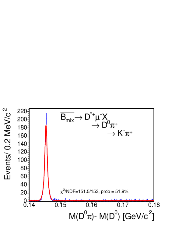
Figure 5.1: $M_{D^{0}\pi}-M_{D^{0}}$ from the $D^{*}\mu$ events fit to a double- Gaussian signal and a constant background. The result of the unbinned likelihood fit is projected on the histogram and a $\chi^{2}$ probability is calculated.

5.1.2 $D\mu$ Yield

A first glance of $M_{K\pi\pi}$ in Figure 4.5 (middle right) might suggest that we could fit $M_{K\pi\pi}$ to a Gaussian signal and a first-order polynomial background. But, since we do not apply particle identification (PID) in this analysis, the background under the signal contains not only the combinatorial background, but also contamination from the $D_{s}$ decays. Not using PID means that a pion mass might be assigned to a kaon, and $D_{s}^{+}$ may be reconstructed as $D^{+}$. Figure 5.2 shows the mis-reconstructed $D^{+}$ mass spectrum from the $\overline{B}_{s}\rightarrow D_{s}^{+}\mu^{-}\overline{\nu}_{\mu}$ MC, where $D_{s}$ are forced to decay into the final states listed in Table 5.2. These final states are selected after a study to identify the dominant $D_{s}$ decays reconstructed in the $D^{+}$ mass window. The MC used to assess $D_{s}$ background is produced as described in Section 6.1.

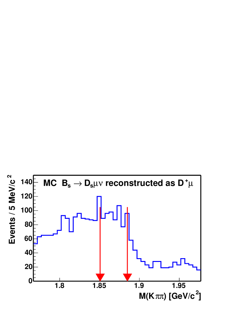
Figure 5.2: $\overline{B}_{s}\rightarrow D_{s}^{+}\mu^{-}\overline{\nu}_{\mu}$ MC reconstructed as $D\mu$ final state. Here $D_{s}$ are forced to decay into the modes listed in Table 5.2. The arrows indicate the 3 $\sigma$ $D^{+}$ signal region.

Table 5.2: Dominant mis-identified $D_{s}$ sequential decays in $D\mu$ signal. Branching fractions without uncertainties have an upper limit in the PDG.

Selected final states of $D_{s}$ decays
Mode	${\cal B}$ ($\%$)		relative to ${\cal B}(D_{s}\rightarrow\phi\pi)$
$D_{s}^{+}\rightarrow\phi\pi^{+}$	3.6 $\pm$	0.9	1
$D_{s}^{+}\rightarrow\phi K^{+}$	0.03 $\pm$	?	0.008 $\pm$	?
$D_{s}^{+}\rightarrow\eta\pi^{+}$	1.7 $\pm$	0.5	0.48 $\pm$	0.05
$D_{s}^{+}\rightarrow\eta^{\prime}\pi^{+}$	3.9 $\pm$	1.0	1.08 $\pm$	0.09
$D_{s}^{+}\rightarrow\omega\pi^{+}$	0.28 $\pm$	0.11	0.077 $\pm$	0.025
$D_{s}^{+}\rightarrow\rho^{0}\pi^{+}$	0.04 $\pm$	?	0.011 $\pm$	?
$D_{s}^{+}\rightarrow\rho^{0}K^{+}$	0.15 $\pm$	?	0.042 $\pm$	?
$D_{s}^{+}\rightarrow f_{0}\pi^{+}$	0.57 $\pm$	0.17	0.16 $\pm$	0.03
$D_{s}^{+}\rightarrow f_{2}\pi^{+}$	0.35 $\pm$	0.12	0.098 $\pm$	0.022
$D_{s}^{+}\rightarrow\rho^{+}\eta$	10.8 $\pm$	3.1	2.98 $\pm$	0.44
$D_{s}^{+}\rightarrow\rho^{+}\eta^{\prime}$	10.1 $\pm$	2.8	2.78 $\pm$	0.41
$D_{s}^{+}\rightarrow\overline{K}^{0}\pi^{+}$	0.4 $\pm$	?	0.11 $\pm$	?
$D_{s}^{+}\rightarrow\overline{K}^{*0}\pi^{+}$	0.65 $\pm$	0.28	0.18 $\pm$	0.06
$D_{s}^{+}\rightarrow K^{0}K^{+}$	3.6 $\pm$	1.1	1.01 $\pm$	0.16
$D_{s}^{+}\rightarrow K^{*0}K^{+}$	3.3 $\pm$	0.9	0.92 $\pm$	0.09
$D_{s}^{+}\rightarrow\pi^{+}\pi^{+}\pi^{-}$	0.005 $\pm$	${+0.022\atop-0.005}$	0.0014 $\pm$	0.0007
$D_{s}^{+}\rightarrow K^{+}K^{-}\pi^{+}$	0.9 $\pm$	0.4	0.25 $\pm$	0.09
$D_{s}^{+}\rightarrow K^{+}K^{+}K^{-}$	0.02 $\pm$	?	0.0056 $\pm$	?

We need to include the mis-identified $D_{s}$ mass shape in our likelihood fit so to properly estimate the number of $D\mu$ events in the data. Assuming that $\overline{B}\rightarrow D_{s}^{+}\mu^{-}X$ has a similar mass spectrum as $\overline{B}_{s}\rightarrow D_{s}^{+}\mu^{-}\overline{\nu}_{\mu}$, we could use the MC for Figure 5.2 to obtain the function which describes the line-shape of mis-reconstructed $D_{s}$ mass spectrum. We find the $D_{s}$ spectrum (${\cal F}$) could be described by a constant and a triangular function convoluted with a Gaussian (${\cal T}$):

$${\cal F}(m)=(1-f_{\mathrm{trg}})\cdot\frac{1}{M_{\mathrm{max}}-M_{\mathrm{min}}}+f_{\mathrm{trg}}\cdot{\cal T}(m),$$ (5.4)

where $f_{\mathrm{trg}}$ is the fraction of triangular function, $M_{\mathrm{max}}$ and $M_{\mathrm{min}}$ specify the mass window, 1.767 $<$ $M_{K\pi\pi}$ $<$ 1.977 ${\rm GeV}/{\rm c}^{2}$, and

$${\cal T}(m)={\frac{2(m-M_{0})}{(M_{\mathrm{off}}-M_{0})^{2}}}\otimes{\cal G}(m,M_{0},\sigma_{\mathrm{trg}}).$$ (5.5)

Here, $\otimes$ represents convolution, $\cal G$ is the Gaussian and $\sigma_{\mathrm{trg}}$ is the width of ${\cal G}$. The triangular function value starts from zero at $M_{0}$ and increases as the mass increases. When the mass reaches $M_{\mathrm{off}}$, the function values is at its maximum and drops precipitously to zero. A graphical representation of $M_{\mathrm{off}}$ and $M_{0}$ may be found in Figure 5.4. The exact form of ${\cal T}(m)$ is found in the appendix of Yu [65] derived by Heinrich. Figure 5.4 shows the result of the fit to the MC.

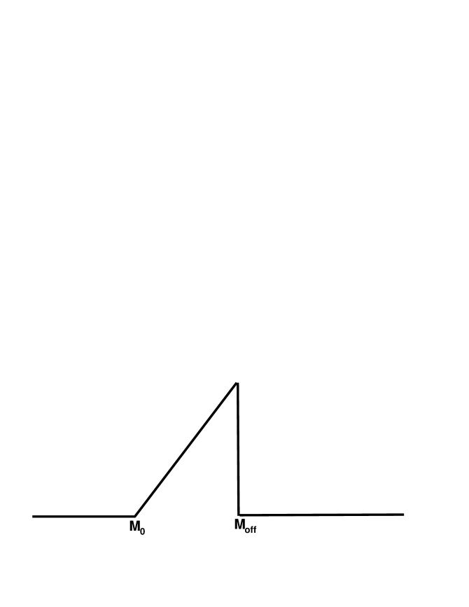
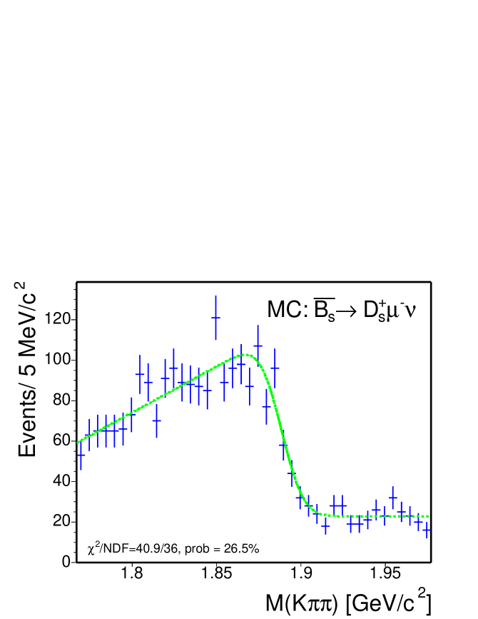
Figure 5.3: Graphical representation of the triangular function.

Figure 5.4: Mis-reconstructed $D_{s}$ from the $\overline{B}_{s}\rightarrow D_{s}^{+}\mu^{-}\overline{\nu}_{\mu}$ MC fit to a constant and a triangular function convoluted with a Gaussian. The dashed curve indicates the result of the unbinned likelihood fit.

Now with the function form of the $M_{K\pi\pi}$ spectrum from the $D_{s}$ decays, we have to normalize the MC yield to the data. The $D_{s}$ yield may be obtained by reconstructing one of the $D_{s}$ final states in the data: $\overline{B}\rightarrow D_{s}^{+}\mu^{-}X$, where $D_{s}^{+}\rightarrow\phi\pi^{+}$, $\phi\rightarrow K^{+}K^{-}$, then using MC to determine the ratio of this $D_{s}$ decay to that of all the $D_{s}$ decays in Table 5.2, $R_{\phi\pi}$:

$$R_{\phi\pi}=\frac{N_{\phi\pi}^{\mathrm{MC}}}{N_{\mathrm{all}}^{\mathrm{MC}}}.$$ (5.6)

The normalization of $D_{s}$ is then expressed as:

$$N_{\overline{B}\rightarrow D_{s}^{+}\mu^{-}X}=\frac{N_{\overline{B}\rightarrow D_{s}^{+}\mu^{-}X,D_{s}\rightarrow\phi\pi,\phi\rightarrow KK}}{R_{\phi\pi}}.$$ (5.7)

In order to obtain $N_{\overline{B}\rightarrow D_{s}^{+}\mu^{-}X,D_{s}\rightarrow\phi\pi,\phi\rightarrow KK}$ in the data, the same analysis cuts for $D\mu$ are applied, except that we assign kaon mass to one of the same-sign charged tracks and pion mass to the other. We still assign kaon mass to the track which has the opposite charge of the other two. In addition, the candidates are required to pass the following cuts:

• 1.767 $<$ $M_{K\pi\pi}$ $<$ 1.977 ${\rm GeV}/{\rm c}^{2}$

• $|M_{KK}-1.019|<$ 0.01 ${\rm GeV}/{\rm c}^{2}$

The cut on $M_{KK}$ guarantees that there is no mis-identified $D^{+}$ in the $D_{s}^{+}$ signal we reconstruct. We confirm this by reconstructing $D_{s}^{+}$ from the $\overline{B}^{0}\rightarrow D^{+}\mu^{-}\overline{\nu}_{\mu}$ MC and no $D_{s}$ candidate is found. See Figure 5.5 for the $\overline{B}\rightarrow D_{s}^{+}\mu^{-}X$ signal in the data, we find:

$$N_{\overline{B}\rightarrow D_{s}^{+}\mu^{-}X,D_{s}\rightarrow\phi\pi,\phi\rightarrow KK}=237\pm 17.$$

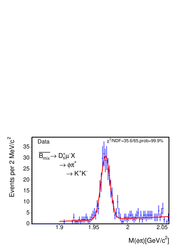
Figure 5.5: Data: Reconstructed $\overline{B}\rightarrow D_{s}^{+}\mu^{-}X$, where $D_{s}^{+}\rightarrow\phi\pi^{+}$, and $\phi\rightarrow K^{+}K^{-}$. $M_{K\pi\pi}$ is required to be between 1.767 and 1.977 GeV/c². There are 237 $\pm$ 17 events in the peak.

We then reconstruct the same $D_{s}$ decay chain in the MC as in the data and obtain

$$R_{\phi\pi}=0.131\pm 0.007.$$ (5.8)

Inserting the result of $N_{\overline{B}\rightarrow D_{s}^{+}\mu^{-}X,D_{s}\rightarrow\phi\pi,\phi\rightarrow KK}$ and $R_{\phi\pi}$ into Equation 5.7, we have:

$$N_{\overline{B}\rightarrow D_{s}^{+}\mu^{-}X}=1812\pm 160,$$ (5.9)

The uncertainty in Equation 5.9 comes from the fractional uncertainties on: $N_{\overline{B}\rightarrow D_{s}^{+}\mu^{-}X,D_{s}\rightarrow\phi\pi,\phi\rightarrow KK}$ (7.2$\%$) and $R_{\phi\pi}$ (5$\%$).

In the unbinned fit, the extended log likelihood function is expressed by the sum of two likelihoods: one describing the data and the other describing the $\overline{B}_{s}\rightarrow D_{s}^{+}\mu^{-}\overline{\nu}_{\mu}$ MC since we fit the data and MC simultaneously;

$$\log{\cal L}=\log{\cal L}^{\mathrm{data}}+\log{\cal L}^{\mathrm{MC}},$$ (5.10)

The likelihood function for the data, $\log{\cal L}^{data}$, is a sum of a signal Gaussian, a first-order polynomial for the combinatorial background (${\cal H}$), and the function for the $D_{s}$ (${\cal F}$, see Equation 5.4). A Gaussian constraint on the amount of $D_{s}$, ${\cal C}_{D_{s}}$, is employed.

$$\log{\cal L}^{\mathrm{data}} = \sum_{i}\log\{N_{\mathrm{sig}}\cdot{\cal G}(m_{i},\mu,\sigma)+N_{\mathrm{combg}}\cdot{\cal H}(m_{i})+N_{D_{s}}\cdot{\cal F}(m_{i})\}$$ (5.11)

$$- N_{\mathrm{sig}}-N_{\mathrm{combg}}-N_{D_{s}}+\log{\cal C}_{D_{s}},$$

where

$${\cal H}(m_{i}) = \frac{1}{M_{\mathrm{max}}-M_{\mathrm{min}}}+p_{1}\cdot(m_{i}-\frac{M_{\mathrm{max}}+M_{\mathrm{min}}}{2}),$$

$${\cal C}_{D_{s}} = {\cal G}(N_{D_{s}},\mu^{p},\sigma^{p}).$$

From the prediction of Equation 5.9, we have $\mu^{p}=1812$, and $\sigma^{p}=160$.

The likelihood function $\log{\cal L}^{\mathrm{MC}}$ is used to fit $\overline{B}_{s}\rightarrow D_{s}^{+}\mu^{-}\overline{\nu}_{\mu}$ MC and obtain the parameterization of ${\cal F}(m)$. Here the normalization does not matter.

$$\log{\cal L}^{\mathrm{MC}}=\sum_{i}\log\{{\cal F}(m_{i})\}.$$ (5.12)

Table 5.3 lists the mean, width of the pulls from 1000 toy MC test and the result returned from the unbinned likelihood fit to the data. Figure 5.6 shows the fit result superimposed on the data histogram. We have obtained from the fit:

$$N_{\overline{B}\rightarrow D^{+}\mu^{-}X}=4720\ \pm 100.$$

We also perform a cross-check by removing the constraint on $N_{D_{s}}$ and obtain $N_{\overline{B}\rightarrow D^{+}\mu^{-}X}=4667\pm 139$, $N_{D_{s}}=2184\pm 620$, which are consistent with the result of the constrained fit. The fit without constraint has a $\chi^{2}/\mathrm{NDF}$=197.0/199 and probability is 52.7$\%$.

Table 5.3: $D\mu$ results from the unbinned likelihood fit.

Index	Parameter		1000 toy MC	1000 toy MC	Data fit value
			pull mean	pull width
1	$N_{\mathrm{sig}}$		-0.012 $\pm$ 0.035	1.004 $\pm$ 0.025	$4720\ \pm 100$
2	$\mu$	[${\rm GeV}/{\rm c}^{2}$]	0.027 $\pm$ 0.037	1.048 $\pm$ 0.027	1.8680 $\pm$ 0.0002
3	$\sigma$	[${\rm GeV}/{\rm c}^{2}$]	0.007 $\pm$ 0.035	0.992 $\pm$ 0.025	0.0084 $\pm$ 0.0002
4	$N_{\mathrm{combg}}$		-0.076 $\pm$ 0.038	1.073 $\pm$ 0.027	15178 $\pm$ 197
5	$p_{1}$		0.018 $\pm$ 0.036	1.027 $\pm$ 0.026	-5.2 $\pm$ 0.7
6	$N_{D_{s}}$		0.042 $\pm$ 0.037	1.065 $\pm$ 0.027	1832 $\pm$ 155
7	$f_{\mathrm{trg}}$		0.022 $\pm$ 0.036	1.023 $\pm$ 0.026	0.617 $\pm$ 0.021
8	$M_{0}$	[${\rm GeV}/{\rm c}^{2}$]	0.055 $\pm$ 0.035	1.007 $\pm$ 0.025	1.69 $\pm$ 0.02
9	$M_{\mathrm{off}}$	[${\rm GeV}/{\rm c}^{2}$]	-0.025 $\pm$ 0.036	1.019 $\pm$ 0.026	1.888 $\pm$ 0.002
10	$\sigma_{\mathrm{trg}}$	[${\rm GeV}/{\rm c}^{2}$]	-0.035 $\pm$ 0.037	1.056 $\pm$ 0.027	0.010 $\pm$ 0.002

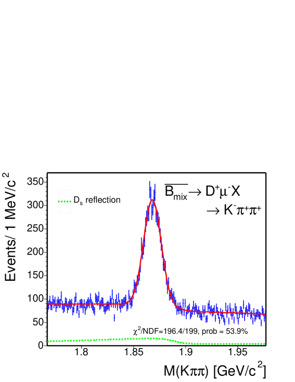
Figure 5.6: $M_{K\pi\pi}$ from the $D\mu$ events fit to a Gaussian (signal), a first-order polynomial (combinatorial background), and a constant plus a triangular function convoluted with a Gaussian (marked by the dashed line). The result of the unbinned likelihood fit is projected on the histogram and a $\chi^{2}$ probability is calculated.

5.1.3 $\Lambda_{c}\mu$ Yield

When a proton mass is assigned to a kaon or pion, numerous $B$ meson to $D$ meson semileptonic decays could be mis-reconstructed as a $\Lambda_{c}\mu$ final state. In order to estimate the $B$ meson background shape under our signal, we use generator level MC and generate the semileptonic decays ($\mu$ channel) of each $B$ meson flavor separately. After applying analysis cuts, we add up the mis-reconstructed mass spectrum from each kind of $B$ meson according to the production fractions:

$b\rightarrow B_{d}$ = (39.7 $\pm$ 1.3) $\%$,

$b\rightarrow B_{u}$ = (39.7 $\pm$ 1.3) $\%$,

$b\rightarrow B_{s}$ = (10.7 $\pm$ 1.1) $\%$.

Figure 5.8 shows a smooth mass spectrum from the generator MC. The shape is best described by a second-order polynomial, with $\chi^{2}/\mathrm{NDF}$ = 36.6/42, prob = 70$\%$. A first-order polynomial fit yields $\chi^{2}/\mathrm{NDF}$ = 56.6/43, prob = 8$\%$. Because the combinatorial background may be parameterized by a first-order polynomial, and adding a first- to a second-order polynomial gives a second-order polynomial, we fit the combinatorial and the $B$ meson background together to a second-order polynomial (${\cal H}$). The extended log likelihood function could be expressed as:

$$\log{\cal L}=\sum_{i}\log\{N_{\mathrm{sig}}\cdot{\cal G}(m_{i},\mu,\sigma)+N_{\mathrm{bg}}\cdot{\cal H}(m_{i})\}-N_{\mathrm{sig}}-N_{\mathrm{bg}},$$ (5.13)

where

$${\cal H}(m_{i})=\frac{1}{M_{\mathrm{max}}-M_{\mathrm{min}}}+p_{1}\cdot(m_{i}-M_{\mathrm{mid}})+p_{2}\cdot(12\cdot(m_{i}-M_{\mathrm{mid}})^{2}-M_{\mathrm{diff}}^{2}).$$

Here, $M_{\mathrm{max}}$ and $M_{\mathrm{min}}$ specify the $\Lambda_{c}^{+}$ mass window: 2.19 $<$ $M_{pK\pi}$ $<$ 2.37 ${\rm GeV}/{\rm c}^{2}$. The average of $M_{\mathrm{max}}$ and $M_{\mathrm{min}}$, or the mid point in the mass window is $M_{\mathrm{mid}}$. The difference of $M_{\mathrm{max}}$ and $M_{\mathrm{min}}$ is $M_{\mathrm{diff}}$. Table 5.4 lists the mean, width of the pulls from the toy MC test and the parameter value from the fit to the data. Figure 5.8 shows fit result superimposed on the data histogram. We have obtained from the fit:

$$N_{\overline{B}\rightarrow\Lambda_{c}^{+}\mu^{-}X}=1237\ \pm 97.$$

Table 5.4: $\Lambda_{c}\mu$ results from the unbinned likelihood fit.

Index	Parameter		1000 toy MC	1000 toy MC	Data fit value
			pull mean	pull width
1	$N_{\mathrm{sig}}$		0.018 $\pm$ 0.030	0.997 $\pm$ 0.022	$1237\ \pm 97$
2	$\mu$	[${\rm GeV}/{\rm c}^{2}$]	0.017 $\pm$ 0.033	1.070 $\pm$ 0.024	2.2850 $\pm$ 0.0005
3	$\sigma$	[${\rm GeV}/{\rm c}^{2}$]	-0.069 $\pm$ 0.032	1.036 $\pm$ 0.023	0.0074 $\pm$ 0.0006
4	$N_{\mathrm{bg}}$		0.004 $\pm$ 0.031	1.021 $\pm$ 0.022	16576 $\pm$ 157
5	$p_{1}$		0.010 $\pm$ 0.031	1.007 $\pm$ 0.022	-4.3 $\pm$ 0.8
6	$p_{2}$		0.020 $\pm$ 0.031	1.012 $\pm$ 0.022	-3.7 $\pm$ 1.8

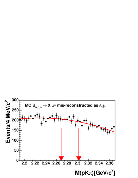
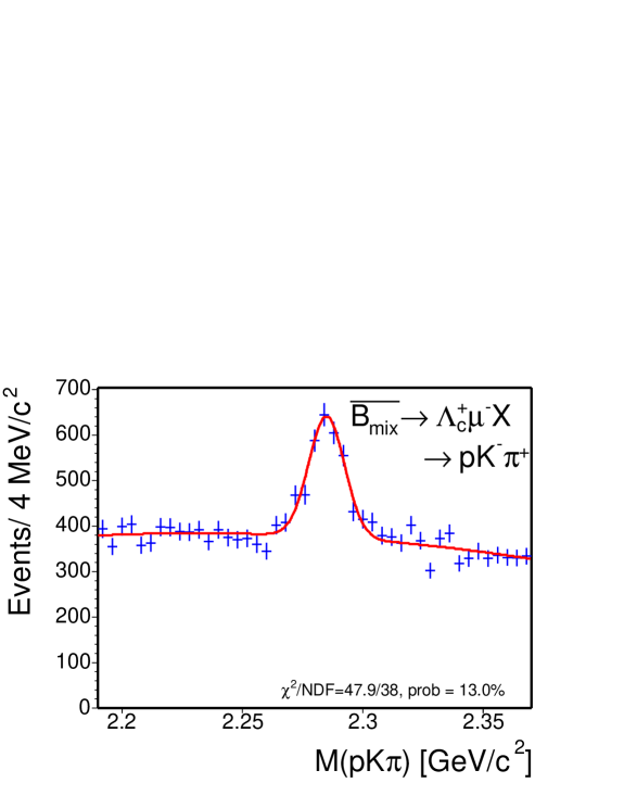
Figure 5.7: $B\rightarrow X\mu\nu_{\mu}$ MC mis-reconstructed as $\Lambda_{c}\mu$. The mass spectrum fit to a second-order polynomial. $\chi^{2}/\mathrm{NDF}$ = 36.6/42, prob= 70.7$\%$. Two arrows indicate the signal region of $\Lambda_{c}^{+}$.

Figure 5.8: $M_{pK\pi}$ from the $\Lambda_{c}\mu$ events fit to a Gaussian (signal), a second-order polynomial (combinatorial + $B$ meson). The result of the unbinned likelihood fit is projected on the histogram and a $\chi^{2}$ probability is calculated.

5.2 Mass Fit of the Hadronic Modes

Figure 4.5 shows that to the left of the hadronic signal peak, the “charm+$\pi$” mass spectrum exhibits an interesting structure. In order to extract a correct number of events observed in the hadronic channels, we have to take into account the background structure when fitting the charm+$\pi$ mass spectrum. For the $\overline{B}^{0}\rightarrow D^{+}\pi^{-}$ and $\Lambda_{b}\rightarrow\Lambda_{c}^{+}\pi^{-}$ modes, we import the $B^{0}$ and $\Lambda_{b}$ mass functions derived in the analyses of Furic [67], and Maksimović [68], respectively. Several parameters that describe the background shapes or normalizations are fixed. We find small modifications are needed for the numerical values of the fixed parameters in the $\overline{B}^{0}\rightarrow D^{+}\pi^{-}$ mode, as a few variables we apply cut on are different from those in Furic’s analysis. We apply our cuts on the MC used in Furic’s analysis and refit the MC to extract the numbers for our analysis. For the $\overline{B}^{0}\rightarrow D^{*+}\pi^{-}$ mode, we produce an inclusive $B\rightarrow D^{*+}X$ MC sample to study the background composition. The decay modes with distinguished mass shape are separated from the other modes. The decays with similar mass spectra are lumped together and fit to the same background function. Figure  5.9 shows the $B^{0}$ and $\Lambda_{b}$ mass spectra from the contributions of different decays.

Our hadronic mass spectra share several common features: It is clear that the background from the $B$ hadron decays only contribute to the mass region below the signal, while in the data, the upper mass region is composed of combinatorial background, which may be described by an exponential or a constant. The combinatorial background extends down to the lower $B$ mass region as well. In the region 40 to 70 ${\rm MeV}/{\rm c}^{2}$ below the signal peak, Cabibbo suppressed decays, $\overline{B}^{0}\rightarrow D^{*+}K^{-}$, $\overline{B}^{0}\rightarrow D^{+}K^{-}$, $\Lambda_{b}\rightarrow\Lambda_{c}^{+}K^{-}$, with a branching ratio about $8\%$ of our Cabibbo favored signals, produce a small contamination. Going further down in the charm+$\pi$ mass, we have partially reconstructed $B$ decays from the semileptonic modes, and other mis-identified $B$ hadronic decays.

Note that since both $\overline{B}^{0}\rightarrow D^{*+}\pi^{-}$ and $\Lambda_{b}\rightarrow\Lambda_{c}^{+}\pi^{-}$ have low statistics, we constrain the widths of their signal Gaussians in the following way: We first fit the width of $M_{D\pi}$ ($\sigma^{\mathrm{data}}_{D\pi}$) from the high statistics $\overline{B}^{0}\rightarrow D^{+}\pi^{-}$ sample ($\sim$600 events) in the data. Then we multiply $\sigma^{\mathrm{data}}_{D\pi}$ with the MC width ratio: $\sigma^{\mathrm{MC}}_{\Lambda_{c}\pi,D^{*}\pi}/\sigma^{\mathrm{MC}}_{D\pi}$ and predict $\sigma^{\mathrm{data}}_{\Lambda_{c}\pi,D^{*}\pi}$.

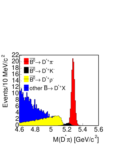
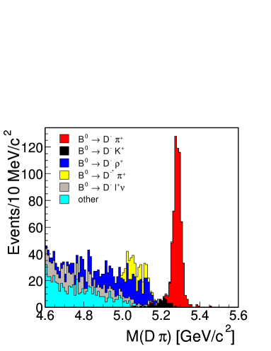
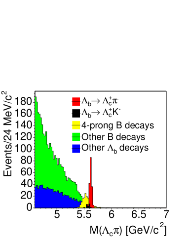
Figure 5.9: Background composition for $\overline{B}^{0}\rightarrow D^{*+}\pi^{-}$ (top), $\overline{B}^{0}\rightarrow D^{+}\pi^{-}$ (middle) from Furic [67] and $\Lambda_{b}\rightarrow\Lambda_{c}^{+}\pi^{-}$ (bottom) from Maksimović [68]. Note that the mis-reconstructed $\overline{B}_{s}\rightarrow D_{s}^{+}\pi^{-}$ and $\Lambda_{b}\rightarrow\Lambda_{c}^{+}\pi^{-}$ in the $D\pi$ mass is not shown.

5.2.1 $\overline{B}^{0}\rightarrow D^{*+}\pi^{-}$ Yield

The study from the $\overline{B}\rightarrow D^{*+}X$ MC shows that the background in the lower mass region is dominated by the following decays: Cabibbo suppressed decay $\overline{B}^{0}\rightarrow D^{*+}K^{-}$, $\overline{B}^{0}\rightarrow D^{*+}\rho^{-}$, and the remaining $\overline{B}\rightarrow D^{*+}X$. See the texts below for the detailed descriptions.

1. $\overline{B}^{0}\rightarrow D^{*+}K^{-}$: fully reconstructed Cabibbo suppressed decays. The mass spectrum is a peak about 40 ${\rm MeV}/{\rm c}^{2}$ below the $\overline{B}^{0}\rightarrow D^{*+}\pi^{-}$ signal, with small tails on the lower mass side. The shape is modeled by a lifetime function;

   $${\cal E}(m)=\exp(m,\tau_{D^{*}K})\otimes{\cal G}(m,\mu_{D^{*}K},\sigma_{D^{*}K}),$$ (5.14)

   where $\tau_{D^{*}K}$ is the lifetime, $\mu_{D^{*}K}$ is the zero point of the lifetime function also the mean of the Gaussian. The width of the Gaussian also the resolution of the lifetime function is $\sigma_{D^{*}K}$. The exact form of ${\cal E}(m)$ is found in the appendix of Yu [65]. See Figure 5.10 (top) for the fit to $\overline{B}^{0}\rightarrow D^{*+}K^{-}$ MC.

2. $\overline{B}^{0}\rightarrow D^{*+}\rho^{-}$, where $\rho^{-}\rightarrow\pi^{0}\pi^{-}$: modeled by a triangular function convoluted with a Gaussian;

   $${\cal T}(m)={\frac{2(m-M_{0}^{D^{*}\rho})}{(M_{\mathrm{off}}^{D^{*}\rho}-M_{0}^{D^{*}\rho})^{2}}}\otimes{\cal G}(m,M_{0}^{D^{*}\rho},\sigma_{D^{*}\rho}).$$ (5.15)

   See Figure 5.10 (middle) for the fit.

3. Continuum: remaining $\overline{B}\rightarrow D^{*+}X$ decays partially reconstructed. These backgrounds have similar mass spectrum and are group together. The shape is modeled by a first-order polynomial with a negative slope and a turn-off at $M_{\mathrm{off}}^{\mathrm{otherB}}$; when $m<M_{\mathrm{off}}^{\mathrm{otherB}}$:

   $${\cal H}(m)=\frac{2}{(M_{\mathrm{off}}^{\mathrm{otherB}}-M_{\mathrm{min}})^{2}}\cdot(M_{\mathrm{off}}^{\mathrm{otherB}}-m),$$ (5.16)

   and when $m>M_{\mathrm{off}}^{\mathrm{otherB}}$:

   $${\cal H}(m)=0.$$ (5.17)

   The lowest boundary of the $D^{*}\pi$ mass window, $M_{\mathrm{min}}$, is 4.6 ${\rm GeV}/{\rm c}^{2}$. See Figure 5.10 (bottom) for the fit to these MC samples.

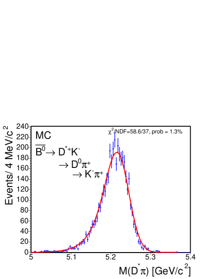
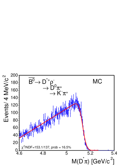
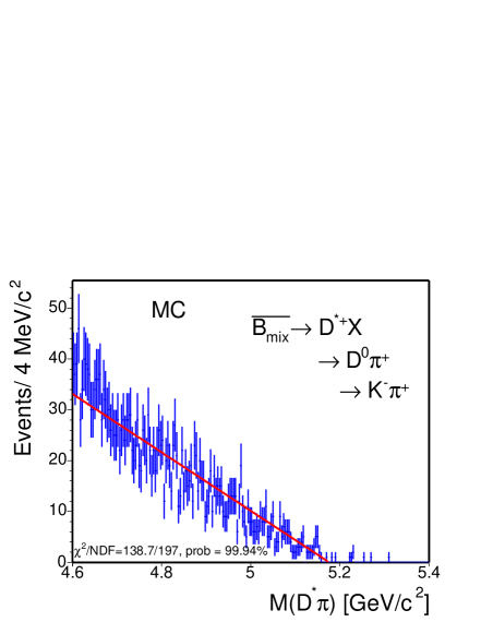
Figure 5.10: Various MC samples reconstructed as $\overline{B}^{0}\rightarrow D^{*+}\pi^{-}$. From the top to the bottom are $\overline{B}^{0}\rightarrow D^{*+}K^{-}$, $\overline{B}^{0}\rightarrow D^{*+}\rho^{-}$, and the remaining $\overline{B}\rightarrow D^{*+}X$.

In the unbinned fit, the extended log likelihood function is expressed by the sum of five likelihoods: one describing the data, and the other four describing the MC samples from each type of background and the signal:

$$\log{\cal L}=\log{\cal L}^{\mathrm{data}}+\log{\cal L}^{\mathrm{MC}}_{D^{*}\pi}+\log{\cal L}^{\mathrm{MC}}_{D^{*}K}+\log{\cal L}^{\mathrm{MC}}_{D*\rho}+\log{\cal L}^{\mathrm{MC}}_{\mathrm{otherB}},$$ (5.18)

The likelihood function $\log{\cal L}^{\mathrm{data}}$ is a sum of a signal Gaussian, a constant combinatorial background, the functions for $D^{*}K$ (${\cal E}$), $D^{*}\rho$ (${\cal T}$), and the continuum (${\cal H}$). In addition, there is a constraint on each of the following parameters: the signal width, relative amount of $D^{*}K$ to the signal ($f_{D^{*}K}$), and the fraction of $D^{*}\rho$ in $D^{*}\rho$ + remaining $\overline{B}\rightarrow D^{*+}X$ ($f_{D^{*}\rho}$) The reason for the last constraint is because $\overline{B}^{0}\rightarrow D^{*+}\rho^{-}$ and the remaining $\overline{B}\rightarrow D^{*+}X$ decays occupy the same mass region. Therefore, the likelihood fit converges faster if we constrain $f_{D^{*}\rho}$.

$$\log{\cal L}^{\mathrm{data}} = \sum_{i}\log\{N_{\mathrm{sig}}\cdot({\cal G}(m_{i},\mu,\sigma)+f_{D^{*}K}\cdot{\cal E}(m_{i}))$$ (5.19)

$$+N_{\mathrm{bg}}\cdot[f_{\mathrm{combg}}\cdot\frac{1}{M_{\mathrm{max}}-M_{\mathrm{min}}}$$

$$+(1-f_{\mathrm{combg}})\cdot[f_{D^{*}\rho}\cdot{\cal T}(m_{i})+(1-f_{D^{*}\rho})\cdot{\cal H}(m_{i})]\}$$

$$- N_{\mathrm{sig}}-N_{D^{*}K}-N_{\mathrm{bg}}$$

$$+ \log{\cal C}_{1}+\log{\cal C}_{2}+\log{\cal C}_{\sigma},$$

where ${\cal E}(m_{i})$, ${\cal T}(m_{i})$ and ${\cal H}(m_{i})$ are expressed in Equations 5.14–5.16. The $M_{\mathrm{max}}$ and $M_{\mathrm{min}}$ specify the mass window: 4.6 $<$ $M_{D^{*}\pi}$ $<$ 5.6 ${\rm GeV}/{\rm c}^{2}$. The parameters $f_{D^{*}K}$, $N_{\mathrm{bg}}$, $f_{\mathrm{combg}}$ and $f_{D^{*}\rho}$ are defined as follow:

$$f_{D^{*}K} \equiv \frac{N_{D^{*}K}}{N_{\mathrm{sig}}},$$

$$N_{\mathrm{bg}} \equiv N_{\mathrm{combg}}+N_{\mathrm{otherB}}+N_{D^{*}\rho},$$

$$f_{\mathrm{combg}} \equiv \frac{N_{\mathrm{combg}}}{N_{\mathrm{bg}}},$$

$$f_{D^{*}\rho} \equiv \frac{N_{D^{*}\rho}}{N_{\mathrm{otherB}}+N_{D^{*}\rho}}.$$

The constraints are expressed as:

$${\cal C}_{1} = {\cal G}(f_{D^{*}K},\mu_{1},\sigma_{1}),$$

$${\cal C}_{2} = {\cal G}(f_{D^{*}\rho},\mu_{2},\sigma_{2}),$$

$${\cal C}_{\sigma} = {\cal G}(\sigma,\mu_{p},\sigma_{p}),$$

where $\mu_{1}=0.071$, $\sigma_{1}=0.019$, $\mu_{2}=0.242$, $\sigma_{2}=0.008$, $\mu_{p}=0.0259\;{\rm GeV}/{\rm c}^{2}$, and $\sigma_{p}=0.0012\;{\rm GeV}/{\rm c}^{2}$.

Here, $\mu_{p}$ and $\sigma_{p}$ are determined using the $\overline{B}^{0}\rightarrow D^{+}\pi^{-}$ signal in the data, $\overline{B}^{0}\rightarrow D^{+}\pi^{-}$ and $\overline{B}^{0}\rightarrow D^{*+}\pi^{-}$ MC as described earlier. The $\mu_{1}$ and $\sigma_{1}$ are determined using the world average branching ratios, and the efficiencies from the MC listed in Table 5.5:

$$f_{D^{*}K}=\frac{{\cal B}(\overline{B}^{0}\rightarrow D^{*+}K^{-})}{{\cal B}(\overline{B}^{0}\rightarrow D^{*+}\pi^{-})}\cdot\frac{\epsilon_{\overline{B}^{0}\rightarrow D^{*+}K^{-}}}{\epsilon_{\overline{B}^{0}\rightarrow D^{*+}\pi^{-}}}.$$ (5.20)

The $\mu_{2}$ and $\sigma_{2}$ are determined by counting the number of reconstructed $D^{*}\rho$ and the remaining $\overline{B}\rightarrow D^{*+}X$ events in the MC after all the analysis cuts.

Table 5.5: Branching ratios and relative efficiencies for $\overline{B}^{0}\rightarrow D^{*+}\pi^{-}$ background.

	$\overline{B}^{0}\rightarrow D^{*+}K^{-}$	$\overline{B}^{0}\rightarrow D^{*+}\pi^{-}$
B($\%$)	0.276 $\pm$ 0.021	0.020 $\pm$ 0.005
$\epsilon$ ratio	1	1.02 $\pm$ 0.02
$f_{D^{*}K}$	0.071 $\pm$ 0.019
	$\overline{B}^{0}\rightarrow D^{*+}\rho^{-}$	remaining $\overline{B}\rightarrow D^{*+}X$
$N_{MC}$	758	2371
$f_{D^{*}\rho}$	0.242 $\pm$ 0.008

The three likelihoods for the background MC are used to obtain the parameterization of ${\cal E}(m)$, ${\cal T}(m)$, and ${\cal H}(m)$. The normalizations do not matter here.

$$\log{\cal L}^{\mathrm{MC}}_{D^{*}K} = \sum_{i}\log{\cal E}(m_{i}),$$ (5.21)

$$\log{\cal L}^{\mathrm{MC}}_{D*\rho} = \sum_{i}\log{\cal T}(m_{i}),$$ (5.22)

$$\log{\cal L}^{\mathrm{MC}}_{\mathrm{otherB}} = \sum_{i}\log{\cal H}(m_{i}).$$ (5.23)

In addition, $\log{\cal L}^{\mathrm{MC}}_{D^{*}\pi}$ is used to obtain the reconstructed mass difference between MC and data, $m_{\mathrm{diff}}$. In the $\log{\cal L}^{\mathrm{data}}$, all the parameters except the normalization and the resolution parameters ($\sigma$) for the signal Gaussian and the background functions, differ by $m_{\mathrm{diff}}$ from those in the $\log{\cal L}^{\mathrm{MC}}$. The resolutions for all the backgrounds are kept the same between MC and data, while the resolution of the signal Gaussian in the data is a separate free parameter from that in the MC.

We use the total likelihood to fit the data and MC simultaneously. Table 5.6 lists the pull means and widths of toy MC test and the unbinned likelihood fit result to the data. Figure 5.11 shows the fit result superimposed on the data histogram. We have obtained from the fit:

$$N_{\overline{B}^{0}\rightarrow D^{*+}\pi^{-}}=106\ \pm 11.$$

If we remove the constraint on the signal width, we find $N_{\overline{B}^{0}\rightarrow D^{*+}\pi^{-}}=110\pm 11$ and $\sigma_{\mathrm{data}}=0.0295\pm 0.0033{\rm GeV}/{\rm c}^{2}$. Removing the constraint on $f_{D^{*}K}$ gives us $N_{\overline{B}^{0}\rightarrow D^{*+}\pi^{-}}=107\pm 11$ and $f_{D^{*}K}=0.053\pm 0.053$. Removing the constraint on $f_{D^{*}\rho}$ gives us $N_{\overline{B}^{0}\rightarrow D^{*+}\pi^{-}}=107\pm 11$ and $f_{D^{*}\rho}=0.38\pm 0.07$. In conclusion, the un-constrained fits return a value consistent with the constrained fit, but with larger uncertainties. The fit $\chi^{2}/\mathrm{NDF}$ are 20.0/12, 20.8/12, 16.5/12 and the fit probabilities are 6.7$\%$, 5.4 $\%$, 16.9$\%$ for the three different unconstrained fits.

Table 5.6: $\overline{B}^{0}\rightarrow D^{*+}\pi^{-}$ results from the unbinned likelihood fit.

Index	Parameter		1000 toy MC	1000 toy MC	Data fit value
			pull mean	pull width
1	$N_{\mathrm{sig}}$		-0.019 $\pm$ 0.031	0.964 $\pm$ 0.022	$106\ \pm 11$
2	$\mu$	[${\rm GeV}/{\rm c}^{2}$]	0.013 $\pm$ 0.033	1.032 $\pm$ 0.024	5.2772 $\pm$ 0.0002
3	$\sigma_{\mathrm{MC}}$	[${\rm GeV}/{\rm c}^{2}$]	-0.043 $\pm$ 0.033	1.036 $\pm$ 0.024	0.0262 $\pm$ 0.0002
4	$f_{D^{*\rho}}$		-0.009 $\pm$ 0.032	1.006 $\pm$ 0.023	0.244 $\pm$ 0.008
5	$M_{0}^{D^{*}\rho}$	[${\rm GeV}/{\rm c}^{2}$]	0.027 $\pm$ 0.033	0.943 $\pm$ 0.020	4.43 $\pm$ 0.01
6	$M_{off}^{D^{*}\rho}$	[${\rm GeV}/{\rm c}^{2}$]	0.045 $\pm$ 0.032	0.993 $\pm$ 0.023	5.134 $\pm$ 0.001
7	$\sigma_{D^{*}\rho}$	[${\rm GeV}/{\rm c}^{2}$]	-0.077 $\pm$ 0.033	1.001 $\pm$ 0.024	0.026 $\pm$ 0.001
8	$f_{\mathrm{combg}}$		-0.045 $\pm$ 0.032	0.940 $\pm$ 0.023	0.09 $\pm$ 0.03
9	$N_{\mathrm{bg}}$		-0.010 $\pm$ 0.033	1.019 $\pm$ 0.023	428 $\pm$ 21
10	$M_{\mathrm{off}}^{\mathrm{otherB}}$	[${\rm GeV}/{\rm c}^{2}$]	-0.220 $\pm$ 0.031	0.972 $\pm$ 0.022	5.174 $\pm$ 0.004
11	$f_{D^{*}K}$		-0.047 $\pm$ 0.033	1.016 $\pm$ 0.023	0.069 $\pm$ 0.018
12	$\mu_{D^{*}K}$	[${\rm GeV}/{\rm c}^{2}$]	-0.032 $\pm$ 0.033	1.024 $\pm$ 0.024	5.2345 $\pm$ 0.0009
13	$\tau_{D^{*}K}$	[${\rm GeV}/{\rm c}^{2}$]-1	-0.017 $\pm$ 0.032	0.986 $\pm$ 0.023	0.0287 $\pm$ 0.0009
14	$\sigma_{D^{*}K}$	[${\rm GeV}/{\rm c}^{2}$]	0.029 $\pm$ 0.033	1.029 $\pm$ 0.024	0.0254 $\pm$ 0.0006
15	$m_{\mathrm{diff}}$	[${\rm GeV}/{\rm c}^{2}$]	-0.034 $\pm$ 0.032	0.992 $\pm$ 0.023	0.005 $\pm$ 0.003
16	$\sigma_{\mathrm{data}}$	[${\rm GeV}/{\rm c}^{2}$]	-0.050 $\pm$ 0.031	0.971 $\pm$ 0.022	0.026 $\pm$ 0.001

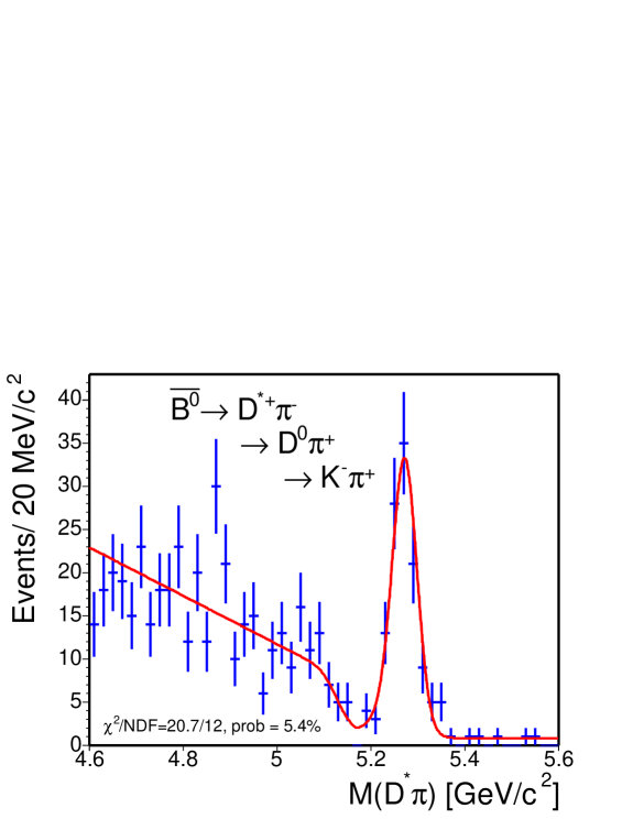
Figure 5.11: $M_{D^{*}\pi}$ from the $\overline{B}^{0}\rightarrow D^{*+}\pi^{-}$ events is fit to a Gaussian (signal), a constant (combinatorial), and the background functions for the lower mass spectrum as described in the text. The result of the unbinned likelihood fit is projected on the histogram and a $\chi^{2}$ probability is calculated. Note that the bins with less than 20 entries are combined.

5.2.2 $\overline{B}^{0}\rightarrow D^{+}\pi^{-}$ Yield

As noted earlier, we make use of the mass function derived in Furic’s analysis for the $\overline{B}^{0}\rightarrow D^{+}\pi^{-}$ mode. The parameters which are kept constant in Furic’s mass function remain constant in our analysis. The following backgrounds contribute to the mass spectrum of $B^{0}$ from Furic’s study: Cabibbo suppressed decay $\overline{B}^{0}\rightarrow D^{+}K^{-}$, $\overline{B}^{0}\rightarrow D^{*+}\pi^{-}$, $\overline{B}^{0}\rightarrow D^{+}\rho^{-}$, remaining $\overline{B}\rightarrow D^{+}X$ and the combinatorial background. Recent study by Belloni, Martin and Piedra et al. [68] [69] shows that the mis-reconstructed $\overline{B}_{s}\rightarrow D_{s}^{+}\pi^{-}$ and $\Lambda_{b}\rightarrow\Lambda_{c}^{+}\pi^{-}$ produce small contamination in the $\overline{B}^{0}\rightarrow D^{+}\pi^{-}$ signal. See the text below for the detailed descriptions.

1. $\overline{B}^{0}\rightarrow D^{+}K^{-}$: fully reconstructed Cabibbo suppressed decays. The mass spectrum is a peak about 60 ${\rm MeV}/{\rm c}^{2}$ below the $\overline{B}^{0}\rightarrow D^{+}\pi^{-}$ signal. The shape is modeled by a single Gaussian;

   $${\cal DK}(m)={\cal G}(m,\mu-\Delta M_{DK},\sigma_{DK}),$$ (5.24)

   where the shift of Gaussian mean from the $\overline{B}^{0}\rightarrow D^{+}\pi^{-}$ signal, $\Delta M_{DK}$, and the width, $\sigma_{DK}$, are extracted from the MC.

2. $\overline{B}_{s}\rightarrow D_{s}^{+}\pi^{-}$, where $D_{s}^{+}\rightarrow\phi\pi^{+}$ and $\phi\rightarrow K^{+}K^{-}$: this decay produces a peak at around 5.31 ${\rm GeV}/{\rm c}^{2}$ when the pion mass is assigned to one of the kaons. The spectrum is modeled by double Gaussians with the same mean;

   $${\cal B_{S}}(m)=f_{1}\cdot{\cal G}(m,\mu_{B_{s}},\sigma_{1})+(1-f_{1})\cdot{\cal G}(m,\mu_{B_{s}},\sigma_{2}),$$ (5.25)

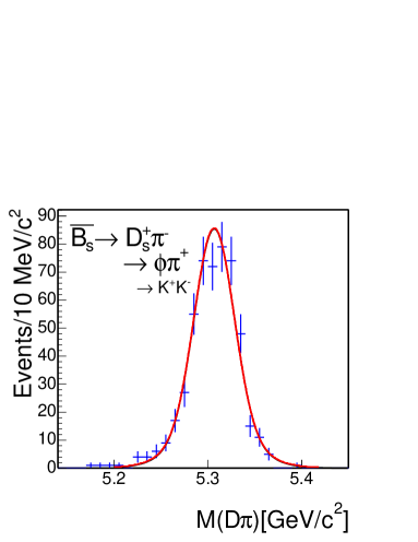
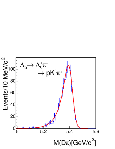
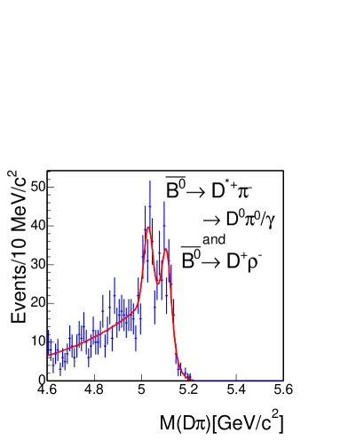
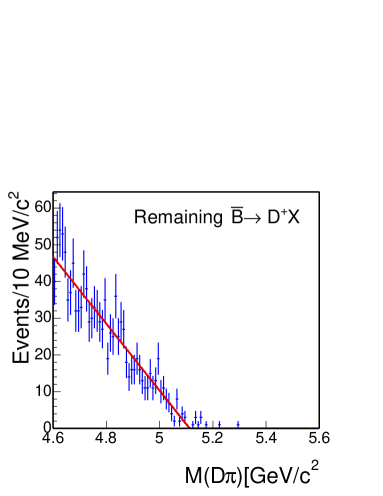
Figure 5.12: Various MC samples reconstructed as $\overline{B}^{0}\rightarrow D^{+}\pi^{-}$. From the top left to the bottom right are $\overline{B}_{s}\rightarrow D_{s}^{+}\pi^{-}$, $\Lambda_{b}\rightarrow\Lambda_{c}^{+}\pi^{-}$, $\overline{B}^{0}\rightarrow D^{*+}\pi^{-}$ + $\overline{B}^{0}\rightarrow D^{+}\rho^{-}$, and the remaining $\overline{B}\rightarrow D^{+}X$. The fit probabilities are 32.5$\%$, 66.8$\%$, 16.5$\%$ and 32.9 $\%$.

   where the fraction $f_{1}$, $\mu_{B_{s}}$, $\sigma_{1}$ and $\sigma_{2}$ of each Gaussian are obtained from the fit to the MC as shown in Figure 5.12 (top left).

3. $\Lambda_{b}\rightarrow\Lambda_{c}^{+}\pi^{-}$, where $\Lambda_{c}^{+}\rightarrow pK^{-}\pi^{+}$: this background produces a broad peak around 5.4 ${\rm GeV}/{\rm c}^{2}$, the region where the pion mass is mis-assigned to the proton. The spectrum is modeled by a lifetime function;

   $${\cal L_{B}}(m)=\exp(m,\tau_{\Lambda_{b}})\otimes{\cal G}(m,\mu_{\Lambda_{b}},\sigma_{\Lambda_{b}}),$$ (5.26)

   where $\mu_{\Lambda_{b}}$ and $\sigma_{\Lambda_{b}}$ are the zero point and the resolution of the lifetime function. See Figure 5.12 (top right) for the fit to the $\Lambda_{b}\rightarrow\Lambda_{c}^{+}\pi^{-}$ MC when reconstructed as $D^{+}\pi^{-}$.

4. $\overline{B}^{0}\rightarrow D^{+}\rho^{-}$, where $\rho^{-}\rightarrow\pi^{0}\pi^{-}$ and $\overline{B}^{0}\rightarrow D^{*+}\pi^{-}$ where $D^{*+}\rightarrow D^{+}\pi^{0}$: These two backgrounds are combined. The spectrum of $\overline{B}^{0}\rightarrow D^{+}\rho^{-}$ looks like $\overline{B}^{0}\rightarrow D^{*+}\rho^{-}$ in Figure 5.10 (middle) and is modeled by a lifetime function. The spectrum of $\overline{B}^{0}\rightarrow D^{*+}\pi^{-}$ is composed of two horns and is modeled by two Gaussians with different means.

   The structure of double horns arises for the following reasons: When $\overline{B}^{0}\rightarrow D^{*+}\pi^{-}$, $D^{*+}\rightarrow D^{+}\pi^{0}$, is reconstructed as $D^{+}\pi^{-}$, the mass is lower than the world average $B^{0}$ mass due to the missing $\pi^{0}$. The amount of the negative mass shift, $\Delta M$, is determined by the angle between the $\pi^{0}$ and the $D^{*+}$ flight direction, $d\phi$. Because both $B^{0}$ and $\pi^{-}$ are scalars (spin=0), to conserve the total angular momentum in the decay, the vector particle (spin=1), $D^{*+}$, is transversely polarized. The angle $d\phi$ from a transversely polarized $D^{*+}$ is $\cos^{2}\theta$ distributed and the most probable $d\phi$ is either 0 or 180 degrees. Therefore, $\Delta M$ is quantized and this forms a double-horns spectrum.

   After combing $\overline{B}^{0}\rightarrow D^{+}\rho^{-}$ and $\overline{B}^{0}\rightarrow D^{*+}\pi^{-}$, we have:

   $${\cal R}(m) = (1-f_{H})\cdot\exp(m,\tau_{\mathrm{ref}})\otimes{\cal G}(m,\mu_{\mathrm{ref}},\sigma_{\mathrm{ref}})$$ (5.27)

   $$+ f_{H}\cdot(0.5\cdot{\cal G}(m,\mu_{\mathrm{ref}}-\nu_{\mathrm{ref}}-\delta_{\mathrm{ref}},\sigma_{H})$$

   $$+0.5\cdot{\cal G}(m,\mu_{\mathrm{ref}}-\nu_{\mathrm{ref}}+\delta_{\mathrm{ref}},\sigma_{H})).$$

   The exact form of the lifetime function is found in the appendix of Yu [65]. The zero point of the lifetime function is $\mu_{\mathrm{ref}}$ and $\nu_{\mathrm{ref}}$ is the offset of the mid point between two horns from the lifetime function. The $\mu_{\mathrm{ref}}$ and $\nu_{\mathrm{ref}}$ are left free in the likelihood fit to the data. The values of the following parameters are extracted from the fit to the MC, as shown in Figure 5.12 (bottom left), and kept constant in the fit to the data: the lifetime ($\tau_{\mathrm{ref}}$), the fraction of horns ($f_{H}$), the half distance between the peak of two horns ($\delta_{\mathrm{ref}}$), the resolution of the lifetime function ($\sigma_{\mathrm{ref}}$) and the width of both horns ($\sigma_{H}$).

5. Continuum: remaining $\overline{B}\rightarrow D^{+}X$ decays and partially reconstructed. These backgrounds have similar mass spectrum and are group together. The shape is modeled by a first-order polynomial with a negative slope and a turn-off at $M_{\mathrm{off}}$; when $m<M_{\mathrm{off}}$:

   $${\cal H}(m)=\frac{2}{(M_{\mathrm{off}}-M_{\mathrm{min}})^{2}}\cdot(M_{\mathrm{off}}-m),$$ (5.28)

   and when $m>M_{\mathrm{off}}$:

   $${\cal H}(m)=0.$$ (5.29)

   The lowest boundary of the $D\pi$ mass window, $M_{\mathrm{min}}$, is 4.6 ${\rm GeV}/{\rm c}^{2}$. See Figure 5.12 (bottom right) for the fit to these MC samples from Furic’s analysis [67].

6. combinatorial: modeled by an exponential function. When the slope of the exponential, $p_{0}$, is not zero,

   $${\cal E_{XP}}(m)=p_{0}\cdot\frac{e^{-p_{0}\cdot M_{\mathrm{mid}}}}{e^{-p_{0}\cdot M_{\mathrm{min}}}-e^{-p_{0}\cdot M_{\mathrm{max}}}}\cdot e^{-p_{0}\cdot(x-M_{\mathrm{mid}})},$$ (5.30)

   and when $p_{0}$ is zero,

   $${\cal E_{XP}}(m)=\frac{1}{M_{\mathrm{max}}-M_{\mathrm{min}}},$$ (5.31)

   where $M_{\mathrm{max}}$ and $M_{\mathrm{min}}$ specify the mass window: 4.6 $<$ $M_{D\pi}$ $<$ 5.6 ${\rm GeV}/{\rm c}^{2}$ and $M_{\mathrm{mid}}$ is the average of $M_{\mathrm{max}}$ and $M_{\mathrm{min}}$.

In the unbinned fit, the extended log likelihood function is expressed as a sum of a signal Gaussian, the functions for the $DK$ mode (${\cal DK}$), $D_{s}\pi$ (${\cal B_{S}}$), $\Lambda_{c}\pi$ (${\cal L_{B}}$), $D^{*}\pi$ plus $D\rho$ (${\cal R}$), the remaining $\overline{B}\rightarrow D^{+}X$ decays (${\cal H}$), and the combinatorial background (${\cal E_{XP}}$):

$$\log{\cal L} = \sum_{i}\log\{N_{\mathrm{sig}}\cdot[{\cal G}(m_{i},\mu,\sigma)+f_{DK}\cdot{\cal DK}(m_{i})$$ (5.32)

$$+f_{B_{s}}\cdot{\cal B_{S}}(m_{i})+f_{\Lambda_{b}}\cdot{\cal L_{B}}(m_{i})]$$

$$+N_{\mathrm{bg}}\cdot[(1-f_{\mathrm{combg}})\cdot[(1-f_{\mathrm{otherB}})\cdot{\cal R}(m_{i})+f_{\mathrm{otherB}}\cdot{\cal H}(m_{i})]$$

$$+f_{\mathrm{combg}}\cdot{\cal E_{XP}}(m_{i})]\}$$

$$- N_{\mathrm{sig}}\cdot(1+f_{DK}+f_{B_{s}}+f_{\Lambda_{b}})-N_{\mathrm{bg}},$$

where ${\cal DK}(m_{i})$, ${\cal B_{S}}(m_{i})$, ${\cal L_{B}}(m_{i})$, ${\cal R}(m_{i})$, ${\cal H}(m_{i})$ and ${\cal E_{XP}}(m_{i})$ are expressed in Equations 5.24–5.31. The fractions $f_{DK}$, $f_{B_{s}}$ and $f_{\Lambda_{b}}$ are the ratios of $N_{DK}$, $N_{B_{s}}$ and $N_{\Lambda_{b}}$ to the signal, $N_{\mathrm{sig}}$. The total amount of combinatorial background, the backgrounds from the $D\rho$, $D^{*}\pi$, and the remaining $B$ decays is denoted as $N_{\mathrm{bg}}$. The parameters $f_{\mathrm{combg}}$ and $f_{\mathrm{otherB}}$ are defined as follows:

$$f_{\mathrm{combg}} \equiv \frac{N_{\mathrm{combg}}}{N_{\mathrm{bg}}},$$

$$f_{\mathrm{otherB}} \equiv \frac{N_{\mathrm{otherB}}}{N_{\mathrm{otherB}}+N_{D^{*}\pi}+N_{D\rho}}.$$

All the fractions and ratios here except $f_{\mathrm{combg}}$ are kept constant in the likelihood fit. The $\overline{B}^{0}\rightarrow D^{+}K^{-}$ fraction, $f_{DK}$, is determined from the world average branching ratios;

$$f_{DK}=\frac{{\cal B}(\overline{B}^{0}\rightarrow D^{+}K^{-})}{{\cal B}(\overline{B}^{0}\rightarrow D^{+}\pi^{-})}.$$ (5.33)

Table 5.9 lists the values of the branching ratios in Equation 5.33. We have $f_{DK}=0.073\pm 0.023$.

The $B_{s}$ fraction, $f_{B_{s}}$, is obtained using the formula:

$$f_{B_{s}} = \frac{f_{s}}{f_{d}}\cdot\frac{{\cal B}(\overline{B}_{s}\rightarrow D_{s}^{+}\pi^{-})}{{\cal B}(\overline{B}^{0}\rightarrow D^{+}\pi^{-})}\cdot\frac{{\cal B}(D_{s}^{+}\rightarrow\phi\pi^{+}){\cal B}(\phi\rightarrow K^{+}K^{-})}{{\cal B}(D^{+}\rightarrow K^{-}\pi^{+}\pi^{+})}$$ (5.34)

$$\cdot\frac{\Gamma(D_{s}^{+}\rightarrow K^{+}K^{-}\pi^{-})}{\Gamma(D_{s}^{+}\rightarrow\phi(K^{+}K^{-})\pi^{-})}\cdot\frac{\epsilon_{\overline{B}_{s}\rightarrow D_{s}^{+}\pi^{-}}^{MC}}{\epsilon_{\overline{B}^{0}\rightarrow D^{+}\pi^{-}}^{MC}},$$

where the branching ratios are from the 2004 PDG and the CDF II measurement $\frac{f_{s}}{f_{d}}\cdot\frac{{\cal B}(\overline{B}_{s}\rightarrow D_{s}^{+}\pi^{-})}{{\cal B}(\overline{B}^{0}\rightarrow D^{+}\pi^{-})}$ by Furic [67]. The efficiency ratio is obtained by applying our $D\pi$ analysis cuts on the $B_{s}$ MC. Inserting the numbers listed in Table 5.9 into Equation 5.34, we obtain $f_{Bs}=0.006\pm 0.001$. Note that the uncertainties from the branching ratios of $\phi$, $D_{s}$, and $D$ decays vanish after multiplying Furic’s result with the ratio: $\frac{{\cal B}(D_{s}^{+}\rightarrow\phi\pi^{+}){\cal B}(\phi\rightarrow K^{+}K^{-})}{{\cal B}(D^{+}\rightarrow K^{-}\pi^{+}\pi^{+})}$.

The $\Lambda_{b}$ fraction, $f_{\Lambda_{b}}$, is obtained using a similar formula;

$$f_{\Lambda_{b}}=\frac{\sigma_{\Lambda_{b}}(P_{T}>6.0){\cal B}(\Lambda_{b}\rightarrow\Lambda_{c}^{+}\pi^{-})}{\sigma_{B^{0}}(P_{T}>6.0){\cal B}(\overline{B}^{0}\rightarrow D^{+}\pi^{-})}\times\frac{{\cal B}(\Lambda_{c}^{+}\rightarrow pK^{-}\pi^{+})}{{\cal B}(D^{+}\rightarrow K^{-}\pi^{+}\pi^{+})}\times\frac{\epsilon_{\Lambda_{b}\rightarrow\Lambda_{c}^{+}\pi^{-}}^{MC}}{\epsilon_{\overline{B}^{0}\rightarrow D^{+}\pi^{-}}^{MC}},$$ (5.35)

where the product of the first and the second terms come from 2004 PDG and CDF II measurements by Le, et al. [68]. The uncertainties from the branching ratios of $\Lambda_{c}$ and $D$ decays vanish in Equation 5.35. The efficiency ratio is obtained using the $\Lambda_{b}\rightarrow\Lambda_{c}^{+}\pi^{-}$ MC. The value of $f_{\Lambda_{b}}$ is then $0.031\pm 0.005$. Table 5.9 lists the numerical values of Le’s result and the MC efficiency. Finally, $f_{\mathrm{otherB}}$ is obtained using Furic’s $\overline{B}\rightarrow D^{+}X$ MC. We apply our analysis cuts and count the number of $D^{*}\pi+D\rho$ and the remaining $\overline{B}\rightarrow D^{+}X$ events. We find $f_{\mathrm{otherB}}=0.569\pm 0.011.$

Table 5.7 lists the constant parameters with their values and uncertainties obtained from the fit to the MC. Table 5.9 lists the mean, width of the pulls from the toy MC test and the value of each fit parameter from the fit to the data. Figure 5.13 shows the fit result superimposed on the data histogram. We have obtained from the fit:

$$N_{\overline{B}^{0}\rightarrow D^{+}\pi^{-}}=579\ \pm 30.$$

Table 5.7: Fixed parameters in the $\overline{B}^{0}\rightarrow D^{+}\pi^{-}$ unbinned likelihood fit.

Parameter	Meaning	Value
$f_{DK}$	$N_{\overline{B}^{0}\rightarrow D^{+}K^{-}}/N_{\overline{B}^{0}\rightarrow D^{+}\pi^{-}}$	0.073 $\pm$	0.023
$\Delta M_{DK}$	mass shift of $\overline{B}^{0}\rightarrow D^{+}K^{-}$ [${\rm GeV}/{\rm c}^{2}$]	0.067 $\pm$	0.006
$\sigma_{DK}$	width of $\overline{B}^{0}\rightarrow D^{+}K^{-}$[${\rm GeV}/{\rm c}^{2}$]	0.032 $\pm$	0.009
$f_{B_{s}}$	$N_{\overline{B}_{s}\rightarrow D_{s}^{+}\pi^{-}}/N_{\overline{B}^{0}\rightarrow D^{+}\pi^{-}}$	0.006 $\pm$	0.001
$\mu_{B_{s}}$	mean of $B_{s}$ background [${\rm GeV}/{\rm c}^{2}$]	5.307 $\pm$	0.001
$f_{1}$	fraction of the narrow $B_{s}$ Gaussian	0.773 $\pm$	0.002
$\sigma_{1}$	width of the narrow $B_{s}$ Gaussian [${\rm GeV}/{\rm c}^{2}$]	0.021 $\pm$	0.002
$\sigma_{2}/\sigma_{1}$	width ratio of the $B_{s}$ Gaussians	1.8 $\pm$	0.3
$f_{\Lambda_{b}}$	$N_{\Lambda_{b}\rightarrow\Lambda_{c}^{+}\pi^{-}}/N_{\overline{B}^{0}\rightarrow D^{+}\pi^{-}}$	0.031 $\pm$	0.005
$\mu_{\Lambda_{b}}$	mean of $\Lambda_{b}$ [${\rm GeV}/{\rm c}^{2}$]	5.416 $\pm$	0.002
$\sigma_{\Lambda_{b}}$	width of $\Lambda_{b}$ background [${\rm GeV}/{\rm c}^{2}$]	0.024 $\pm$	0.002
$\tau_{\Lambda_{b}}$	lifetime of $\Lambda_{b}$ background [${\rm GeV}/{\rm c}^{2}$-1]	0.052 $\pm$	0.002
$\tau_{\mathrm{ref}}$	lifetime of $D\rho$ background [${\rm GeV}/{\rm c}^{2}$-1]	0.36 $\pm$	0.06
$\sigma_{\mathrm{ref}}$	width of $D\rho$ background [${\rm GeV}/{\rm c}^{2}$]	0.039 $\pm$	0.008
$f_{H}$	fraction of $D^{*}\pi$ horns	0.20 $\pm$	0.06
$\delta_{\mathrm{ref}}$	distance between two horns [${\rm GeV}/{\rm c}^{2}$]	0.039 $\pm$	0.003
$\sigma_{H}$	width of the horns [${\rm GeV}/{\rm c}^{2}$]	0.019 $\pm$	0.003
$f_{\mathrm{otherB}}$	fraction of the remaining $\overline{B}\rightarrow D^{+}X$	0.569 $\pm$	0.011
$M_{\mathrm{off}}$	cut off for $\overline{B}\rightarrow D^{+}X$ mass [${\rm GeV}/{\rm c}^{2}$]	5.112 $\pm$	0.007

Table 5.8: Parameter values used to determine $f_{DK}$, $f_{B_{s}}$ and $f_{\Lambda_{b}}$.

${\cal B}(\overline{B}^{0}\rightarrow D^{+}K^{-})$	(2.0 $\pm$ 0.6)$\times 10^{-4}$
${\cal B}(\overline{B}^{0}\rightarrow D^{+}\pi^{-})$	(2.76 $\pm$ 0.25)$\times 10^{-3}$
$f_{DK}$	0.073 $\pm$ 0.023
$\frac{f_{s}}{f_{d}}\cdot\frac{{\cal B}(\overline{B}_{s}\rightarrow D_{s}^{+}\pi^{-})}{{\cal B}(\overline{B}^{0}\rightarrow D^{+}\pi^{-})}$	0.35 $\pm$ 0.05(stat) $\pm$ 0.02 (syst) $\pm$ 0.09 (BR)
${\cal B}(D_{s}^{+}\rightarrow\phi\pi^{+})$	(3.6 $\pm$ 0.9)$\%$
${\cal B}(\phi\rightarrow K^{+}K^{-})$	(49.1 $\pm$ 0.6)$\%$
${\cal B}(D^{+}\rightarrow K^{-}\pi^{+}\pi^{+})$	(9.2 $\pm$ 0.6)$\%$
$\frac{\Gamma(D_{s}^{+}\rightarrow K^{+}K^{-}\pi^{-})}{\Gamma(D_{s}^{+}\rightarrow\phi(K^{+}K^{-})\pi^{-})}$	0.81 $\pm$ 0.08
$\epsilon_{\overline{B}_{s}\rightarrow D_{s}^{+}\pi^{-}}^{MC}/\epsilon_{\overline{B}^{0}\rightarrow D^{+}\pi^{-}}^{MC}$	0.071 $\pm$ 0.004
$f_{B_{s}}$	0.006 $\pm$ 0.001
$\frac{\sigma_{\Lambda_{b}}(P_{T}>6.0){\cal B}(\Lambda_{b}\rightarrow\Lambda_{c}^{+}\pi^{-})}{\sigma_{B^{0}}(P_{T}>6.0){\cal B}(\overline{B}^{0}\rightarrow D^{+}\pi^{-})}$	0.82 $\pm$ 0.08 (stat) $\pm$ 0.11 (syst) $\pm$ 0.22 (BR)
${\cal B}(\Lambda_{c}^{+}\rightarrow pK^{-}\pi^{+})$	(5.0 $\pm$ 1.3)$\%$
$\epsilon_{\Lambda_{b}\rightarrow\Lambda_{c}^{+}\pi^{-}}^{MC}/\epsilon_{\overline{B}^{0}\rightarrow D^{+}\pi^{-}}^{MC}$	0.069 $\pm$ 0.002
$f_{\Lambda_{b}}$	0.031 $\pm$ 0.005

Table 5.9: $\overline{B}^{0}\rightarrow D^{+}\pi^{-}$ results from the unbinned likelihood fit.

Index	Parameter		1000 toy MC	1000 toy MC	Data fit value
			pull mean	pull width
1	$N_{\mathrm{sig}}$		0.012 $\pm$ 0.035	1.021 $\pm$ 0.026	$579\ \pm 30$
2	$\mu$	[${\rm GeV}/{\rm c}^{2}$]	-0.026 $\pm$ 0.034	0.989 $\pm$ 0.025	5.278 $\pm$ 0.001
3	$\sigma$	[${\rm GeV}/{\rm c}^{2}$]	-0.040 $\pm$ 0.035	1.015 $\pm$ 0.026	0.0235 $\pm$ 0.0012
4	$N_{\mathrm{bg}}$		0.017 $\pm$ 0.034	0.990 $\pm$ 0.025	4049 $\pm$ 67
5	$\mu_{\mathrm{ref}}$	[${\rm GeV}/{\rm c}^{2}$]	-0.036 $\pm$ 0.036	1.037 $\pm$ 0.026	5.145 $\pm$ 0.015
6	$\nu_{\mathrm{ref}}$	[${\rm GeV}/{\rm c}^{2}$]	-0.037 $\pm$ 0.038	1.085 $\pm$ 0.028	0.068 $\pm$ 0.020
7	$f_{\mathrm{combg}}$		-0.145 $\pm$ 0.034	0.988 $\pm$ 0.025	0.583 $\pm$ 0.044
8	$p_{0}$		-0.051 $\pm$ 0.034	0.976 $\pm$ 0.024	1.75 $\pm$ 0.15

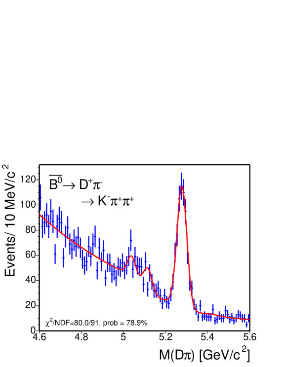
Figure 5.13: $M_{D\pi}$ from the $\overline{B}^{0}\rightarrow D^{+}\pi^{-}$ events is fit to a Gaussian (signal), an exponential (combinatorial), and the background functions for the lower mass spectrum as described in the text. The result of the unbinned likelihood fit is projected on the histogram and a $\chi^{2}$ probability is calculated.

5.2.3 $\Lambda_{b}\rightarrow\Lambda_{c}^{+}\pi^{-}$ Yield

We use the mass function derived in the analysis of Maksimović for the fit to $\Lambda_{b}\rightarrow\Lambda_{c}^{+}\pi^{-}$ data [68]. We cross-check the values of the background shape parameters by applying our analysis cuts on the MC used in the Maksimović analysis. We find the same numbers can be used for this analysis. The following backgrounds contribute to the mass spectrum of $\Lambda_{b}$ from their study: Cabibbo decay $\Lambda_{b}\rightarrow\Lambda_{c}^{+}K^{-}$, four-prong mis-identified $B$ meson, the remaining $B$ meson decays, the remaining $\Lambda_{b}$ decays and the combinatorial background.

1. $\Lambda_{b}\rightarrow\Lambda_{c}^{+}K^{-}$: fully reconstructed Cabibbo suppressed decays. The shape is modeled by two Gaussians of different mean and width;

   $${\cal L_{C}K}(m)=f_{1}\cdot{\cal G}(m,\mu_{\Lambda_{c}K}^{1},\sigma_{1})+(1-f_{1})\cdot{\cal G}(m,\mu_{\Lambda_{c}K}^{2},\sigma_{2}),$$ (5.36)

   where $f_{1}$, $\mu_{\Lambda_{c}K}^{1}$, $\sigma_{1}$, $\mu_{\Lambda_{c}K}^{2}$ and $\sigma_{2}$ are from the fit to the MC.

2. mis-identified four-prong $B$ mesons: all the $B$ mesons with four tracks in the final states and fully reconstructed. $\overline{B}^{0}\rightarrow D^{+}\pi^{-}$ contributes about 50$\%$ of this type of background. Since these decays have similar final state as our $\Lambda_{b}\rightarrow\Lambda_{c}^{+}\pi^{-}$ signal, they produce a distinguished peak to the left of the signal Gaussian. This background (${\cal B}_{4{\cal PRONG}}$) is modeled by the sum of a Landau (${\cal L_{AND}}$) and a Gaussian function:

   $${\cal B}_{4{\cal PRONG}}(m)=f_{\mathrm{L}}\cdot{\cal L_{AND}}(m,\mu_{\mathrm{BPL}},\sigma_{L})+(1-f_{\mathrm{L}})\cdot{\cal G}(m,\mu_{\mathrm{BPG}},\sigma_{G}),$$ (5.37)

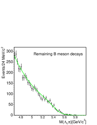
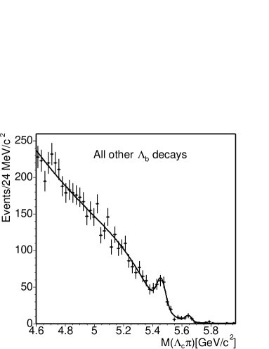
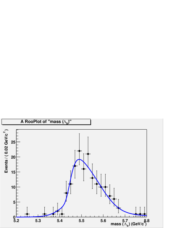
Figure 5.15: Various MC samples reconstructed as $\Lambda_{b}\rightarrow\Lambda_{c}^{+}\pi^{-}$. From the top left to the bottom are the remaining $B$ meson decays, the remaining $\Lambda_{b}$ decays and four-prong $B$ meson decays.

   where $f_{\mathrm{L}}$, $\mu_{\mathrm{BPL}}$ and $\sigma_{L}$ are the fraction, mean and the width of Landau distribution. The mean and the width of the Gaussian are denoted as $\mu_{\mathrm{BPG}}$ and $\sigma_{G}$. These parameters are extracted from fit to the MC as shown in Figure 5.15 (bottom).

3. remaining $B$ meson decays: this background (${\cal O_{B}}$) spectrum is modeled by the sum of an exponential function and a product of a bifurcated Gaussian (${\cal B_{F}}$) with a step-down function:

   $${\cal O_{B}}(m)={\cal E_{XP}}(m)+f_{\mathrm{bifg}}\cdot{\cal B_{F}}(m,\mu_{\mathrm{ob}},\sigma_{\mathrm{ob}}^{L},\sigma_{\mathrm{ob}}^{R})\cdot(1-\frac{1}{1+e^{(\mu_{obst}-m)/a_{0}^{\mathrm{ob}}}})$$ (5.38)

   where ${\cal E_{XP}}(m)$ is expressed in Equations  5.30–5.31. The parameters $f_{\mathrm{bifg}}$, $\mu_{\mathrm{ob}}$, $\sigma_{\mathrm{ob}}^{L}$, and $\sigma_{\mathrm{ob}}^{R}$ are the fraction, mean, left sigma, right sigma of bifurcated Gaussian. The step-down function parameters, $\mu_{obst}$ and $a_{0}^{\mathrm{ob}}$, together with the parameters for the bifurcated Gaussian, are extracted from the MC as shown in Figure 5.15 (top left). The exact form of the bifurcated Gaussian is found in the appendix of Yu [65].

4. remaining $\Lambda_{b}$ decays: this background (${\cal O_{L}}$) spectrum is modeled by the sum of two Gaussians and the product of a bifurcated Gaussian and a step-down function

   $${\cal O_{L}}(m) = f_{1}^{\mathrm{ol}}\cdot{\cal G}(m,\mu_{1}^{olg},\sigma_{1}^{\mathrm{ol}})+f_{2}^{\mathrm{ol}}\cdot{\cal G}(m,\mu_{2}^{olg},\sigma_{2}^{\mathrm{ol}})$$ (5.39)

   $$+\cdot{\cal B_{F}}(m,\mu_{\mathrm{ol}},\sigma_{\mathrm{ol}}^{L},\sigma_{\mathrm{ol}}^{R})\cdot(1-\frac{1}{1+e^{(\mu_{\mathrm{olst}}-m)/a_{0}^{\mathrm{ol}}}})$$

   where the parameters in the function are from the fit to the MC as shown in Figure 5.15 (top right).

5. combinatorial background: described by an exponential function

In the unbinned fit, the extended log likelihood function is expressed as a sum of a signal Gaussian and the functions for $\Lambda_{c}K$ (${\cal L_{C}K}$), four-prong $B$ meson (${\cal B}_{4{\cal PRONG}}$), remaining $B$ meson decays (${\cal O_{B}}$), remaining $\Lambda_{b}$ decays (${\cal O_{L}}$) and the combinatorial background (${\cal E_{XP}}$). In addition, there is a constraint on the width of the signal Gaussian determined using the $\overline{B}^{0}\rightarrow D^{+}\pi^{-}$ data, $\overline{B}^{0}\rightarrow D^{+}\pi^{-}$ and $\Lambda_{b}\rightarrow\Lambda_{c}^{+}\pi^{-}$ MC as described earlier.

$$\log{\cal L} = \sum_{i}\log\{N_{\mathrm{sig}}\cdot[{\cal G}(m_{i},\mu,\sigma)+f_{\Lambda_{c}K}\cdot{\cal L_{C}K}(m_{i})]+N_{\mathrm{B4prong}}\cdot{\cal B}_{4{\cal PRONG}}(m_{i})$$ (5.40)

$$+N_{\mathrm{OB}}\cdot{\cal O_{B}}(m_{i})+N_{\mathrm{OL}}\cdot{\cal O_{L}}(m_{i})+N_{\mathrm{combg}}\cdot{\cal E_{XP}}(m_{i})\}$$

$$- N_{\mathrm{sig}}\cdot(1+f_{\Lambda_{c}K})-N_{\mathrm{B4prong}}-N_{\mathrm{OB}}-N_{\mathrm{OL}}-N_{\mathrm{combg}}+\log{\cal C}_{\sigma},$$

where ${\cal L_{C}K}(m_{i})$, ${\cal B}_{4{\cal PRONG}}(m_{i})$, ${\cal O_{B}}(m_{i})$, ${\cal O_{L}}(m_{i})$ and ${\cal E_{XP}}(m_{i})$ are expressed in Equations 5.36–5.39 and Equations 5.30 –5.31. The fraction $f_{\Lambda_{c}K}$ is defined as:

$$f_{\Lambda_{c}K}=\frac{N_{\Lambda_{b}\rightarrow\Lambda_{c}^{+}K^{-}}}{N_{\Lambda_{b}\rightarrow\Lambda_{c}^{+}\pi^{-}}},$$ (5.41)

and is fixed to 0.08; the number is suggested by the branching ratio of the Cabibbo suppressed relative to the Cabibbo favored decay in the $B$ meson system. The mean and the sigma of the Gaussian constraint for the signal width are $0.0231\;{\rm GeV}/{\rm c}^{2}$, and $0.0012\;{\rm GeV}/{\rm c}^{2}$, respectively.

Table 5.10 lists the mean, width of the pulls from the toy MC test and the fit result to the data. Table 5.11 lists the values of the constant parameters. Figure 5.14 shows the fit result superimposed on the data histogram. We have obtained from the fit:

$$N_{\Lambda_{b}\rightarrow\Lambda_{c}^{+}\pi^{-}}=179\ \pm 19.$$

We also cross-check by removing the constraint on the signal width and obtain $N_{\Lambda_{b}\rightarrow\Lambda_{c}^{+}\pi^{-}}=177\pm 22$, and $\sigma=0.022\pm 0.004$, which are consistent with the result in Table 5.10. The fit without constraint has a $\chi^{2}/\mathrm{NDF}$ of 123.2/111 and fit probability of 20.2 $\%$.

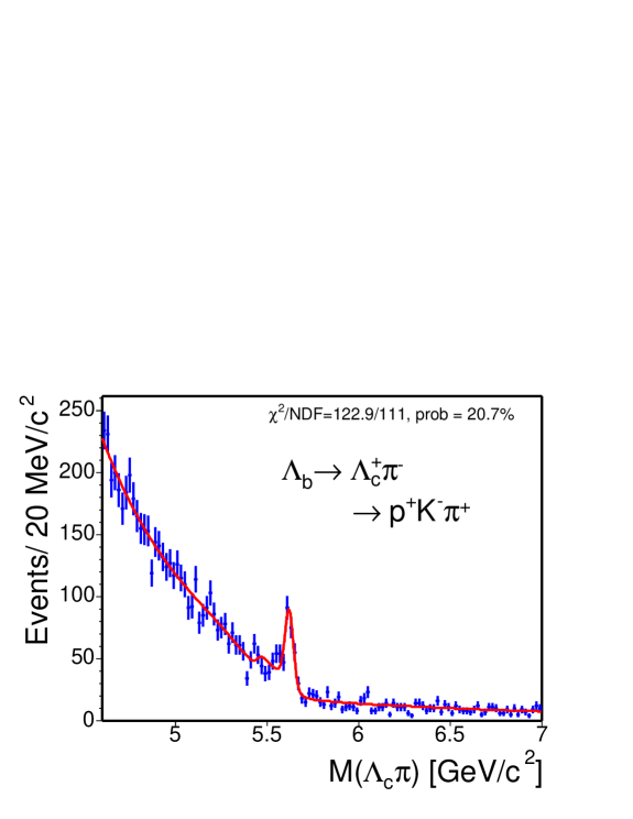
Figure 5.14: $M_{\Lambda_{c}\pi}$ from the $\Lambda_{b}\rightarrow\Lambda_{c}^{+}\pi^{-}$ events is fit to a Gaussian (signal), an exponential (combinatorial), and the background functions for the lower mass spectrum as described in the text. The result of the unbinned likelihood fit is projected on the histogram and a $\chi^{2}$ probability is calculated.

Table 5.10: $\Lambda_{b}\rightarrow\Lambda_{c}^{+}\pi^{-}$ results from the unbinned likelihood fit.

Index	Parameter		1000 toy MC	1000 toy MC	Data fit value
			pull mean	pull width
1	$N_{\mathrm{sig}}$		0.007 $\pm$ 0.032	0.995 $\pm$ 0.023	$179\ \pm 19$
2	$\mu$	[${\rm GeV}/{\rm c}^{2}$]	0.021 $\pm$ 0.033	1.031 $\pm$ 0.024	5.621 $\pm$ 0.003
3	$\sigma$	[${\rm GeV}/{\rm c}^{2}$]	0.026 $\pm$ 0.031	0.976 $\pm$ 0.022	0.023 $\pm$ 0.001
4	$N_{\mathrm{B4prong}}$		0.002 $\pm$ 0.032	1.018 $\pm$ 0.023	150 $\pm$ 32
5	$N_{\mathrm{OB}}$		0.038 $\pm$ 0.033	1.046 $\pm$ 0.024	3170 $\pm$ 291
6	$N_{\mathrm{OL}}$		-0.048 $\pm$ 0.033	1.030 $\pm$ 0.023	962 $\pm$ 324
7	$N_{\mathrm{combg}}$		-0.023 $\pm$ 0.032	1.013 $\pm$ 0.023	1971 $\pm$ 171
8	$p_{0}$		-0.027 $\pm$ 0.032	1.010 $\pm$ 0.023	0.63 $\pm$ 0.10

Table 5.11: Fixed parameters in the $\Lambda_{b}\rightarrow\Lambda_{c}^{+}\pi^{-}$ unbinned likelihood fit.

Parameter	Meaning	Value
$f_{\Lambda_{c}K}$	$N_{\Lambda_{b}\rightarrow\Lambda_{c}^{+}K^{-}}/N_{\Lambda_{b}\rightarrow\Lambda_{c}^{+}\pi^{-}}$	0.080
$f_{1}$	fraction of the narrow $\Lambda_{C}K$ Gaussian	0.902
$\mu_{\Lambda_{c}K}^{1}$	mean of the narrow $\Lambda_{C}K$ Gaussian [${\rm GeV}/{\rm c}^{2}$]	5.573
$\sigma_{1}$	width of the narrow $\Lambda_{C}K$ Gaussian [${\rm GeV}/{\rm c}^{2}$]	0.029
$\mu_{\Lambda_{c}K}^{2}$	mean of the wide $\Lambda_{C}K$ Gaussian [${\rm GeV}/{\rm c}^{2}$]	5.529
$\sigma_{2}$	width of the wide $\Lambda_{C}K$ Gaussian [${\rm GeV}/{\rm c}^{2}$]	0.075
$f_{\mathrm{L}}$	fraction of the Landau, 4-prong	0.413
$\mu_{\mathrm{BPL}}$	mean of the Landau, 4-prong [${\rm GeV}/{\rm c}^{2}$]	5.486
$\sigma_{L}$	width of the Landau, 4-prong [${\rm GeV}/{\rm c}^{2}$]	0.025
$\mu_{\mathrm{BPG}}$	mean of the Gaussian, 4-prong [${\rm GeV}/{\rm c}^{2}$]	5.526
$\sigma_{G}$	width of the Gaussian, 4-prong [${\rm GeV}/{\rm c}^{2}$]	0.078
$s_{0}$	slope of the exponential, other $B$	2.180
$f_{\mathrm{bifg}}$	fraction of the bifurcated Gaus, other $B$	0.106
$\mu_{\mathrm{ob}}$	mean of the bifurcated Gaus, other $B$ [${\rm GeV}/{\rm c}^{2}$]	5.598
$\sigma_{\mathrm{ob}}^{L}$	left $\sigma$ of the bifurcated Gaus, other $B$ [${\rm GeV}/{\rm c}^{2}$]	10.0
$\sigma_{\mathrm{ob}}^{R}$	right $\sigma$ of the bifurcated Gaus, other $B$ [${\rm GeV}/{\rm c}^{2}$]	4.800
$\mu_{obst}$	mean of “step-down”, other $B$ [${\rm GeV}/{\rm c}^{2}$]	5.436
$a_{0}^{\mathrm{ob}}$	slope of the “step-down”, other $B$	0.079
$\mu_{\mathrm{ol}}$	mean of the bifurcated Gaus, other $\Lambda_{b}$ [${\rm GeV}/{\rm c}^{2}$]	3.469
$\sigma_{\mathrm{ol}}^{L}$	left $\sigma$ of the bifurcated Gaus, other $\Lambda_{b}$ [${\rm GeV}/{\rm c}^{2}$]	10.0
$\sigma_{\mathrm{ol}}^{R}$	right $\sigma$ of the bifurcated Gaus, other $\Lambda_{b}$ [${\rm GeV}/{\rm c}^{2}$]	1.236
$\mu_{\mathrm{olst}}$	mean of “step-down”, other $\Lambda_{b}$ [${\rm GeV}/{\rm c}^{2}$]	5.451
$a_{0}^{\mathrm{ol}}$	slope of “step-down”, other $\Lambda_{b}$ [${\rm GeV}/{\rm c}^{2}$]	0.091
$f_{1}^{\mathrm{ol}}$	fraction of first Gaus, other $\Lambda_{b}$	0.0005
$\mu_{1}^{\mathrm{ol}}$	mean of first Gaus, other $\Lambda_{b}$	5.644
$\sigma_{1}^{\mathrm{ol}}$	width of first Gaus, other $\Lambda_{b}$	0.019
$f_{2}^{\mathrm{ol}}$	fraction of second Gaus, other $\Lambda_{b}$	0.0034
$\mu_{2}^{\mathrm{ol}}$	mean of second Gaus, other $\Lambda_{b}$	5.459
$\sigma_{2}^{\mathrm{ol}}$	width of second Gaus, other $\Lambda_{b}$	0.030

5.3 Summary

Using the unbinned, extended log likelihood technique, we fit the charm and $B$ hadron mass spectra to obtain the number of events. The yield for each mode is listed below. The performance of the fitter is validated using 1000 toy MC test for each mode. In general, the mean of each pull distribution from the toy MC test is consistent with zero and the width is consistent with one. For the fit parameter with a pull mean deviated from zero and a width deviated from unity, the fitter only indicates a less than 1$\%$ bias on the central value. Besides, these fit parameters are not correlated with the number of signal events and do not affect the yield we obtain. The fit result to the data is also superimposed on the data histograms and a $\chi^{2}$ is computed. We have obtained good $\chi^{2}$ for each mode.

Mode	Yield
$\overline{B}^{0}\rightarrow D^{*+}\pi^{-}$	$106$  $\pm$	$11$
$\overline{B}\rightarrow D^{*+}\mu^{-}X$	$1059$  $\pm$	$33$
$\overline{B}^{0}\rightarrow D^{+}\pi^{-}$	$579$  $\pm$	$30$
$\overline{B}\rightarrow D^{+}\mu^{-}X$	$4720$  $\pm$	$100$
$\Lambda_{b}\rightarrow\Lambda_{c}^{+}\pi^{-}$	$179$  $\pm$	$19$
$\overline{B}\rightarrow\Lambda_{c}^{+}\mu^{-}X$	$1237$  $\pm$	$97$

Chapter 6 Monte Carlo Samples, Acceptance and Efficiencies

With the raw yield in hand, we now turn to the correction which must be applied to obtain the value of the ratio of branching fractions, that is the acceptance, trigger and reconstruction efficiency which may only be calculated using a Monte Carlo program. The Monte Carlo (MC) simulation plays a crucial role in this analysis. In addition to the acceptance and efficiencies for our signals and backgrounds, as described in Section 6.3 and Chapter 7, the MC is used for the optimization of signals in Section 4.2. MC is also used to find out the function form that describes the mass spectrum of the background due to partial- or mis-reconstruction in Section 5.2. In this chapter, we first explain the components of Monte Carlo samples and show that, in general, the MC reproduces the data. Then we present the acceptance, trigger and reconstruction efficiencies obtained from the MC.

6.1 Monte Carlo Simulation Components

There are several components in the MC simulation:

• production and decay of the $B$ hadrons

• detector simulation

• trigger simulation

Production and Decay of $B$ Hadrons

We use two types of event generators: Bgenerator [70] and PYTHIA [71]. The Bgenerator is the primary generator used in this analysis for calculating the acceptance and efficiencies of our signals and most backgrounds. Bgenerator generates a single $b$-quark according to the $P_{T}(b)$ spectrum which follows the NLO calculation by Nason, Dawson, and Ellis (NDE) [72]. The rapidity of the $b$ quark, $y(b)$, is generated according to $1+q(P_{T})$, where

$$q(P_{T})=-0.0456-0.00289P_{T}.$$ (6.1)

The mass of the $b$ quark is set to 4.75 ${\rm GeV}/{\rm c}^{2}$. For the $B$ meson MC sample, the b-quarks are generated with a $P_{T}$ threshold of 4.0 GeV/c over the range in rapidity $|y|<2.5$, and then fragmented into $B$ mesons with the CDF default Peterson fragmentation parameter [73], $\epsilon_{B}$, set to 0.006. Figure 6.2 shows a small discrepancy in the reconstructed $P_{T}(B^{0})$ between data and MC. The slope of the data to MC ratio is about 2 $\sigma$ away from zero. The MC events which survive the trigger simulation, reconstruction and the analysis cuts, will be re-weighted according to the ratio numerically, i.e. we multiply each event with the ratio, $w$. We then calculate the efficiencies using the re-weighted MC events;

$$R_{\mathrm{pass}}=\sum_{i}^{N_{\mathrm{pass}}}w_{i}$$ (6.2)

$$\epsilon=\frac{R_{\mathrm{pass}}}{N_{\mathrm{gen}}}$$ (6.3)

Figure 6.2 also shows a 4$\sigma$ discrepancy in the reconstructed $P_{T}$($\Lambda_{b}$) between data and MC from the Bgenerator. As the discrepancy is significant, in order to correctly assess the acceptance and efficiency of the $\Lambda_{b}$, the fragmentation process inside Bgenerator has to be turned off. The $\Lambda_{b}$ needs to be generated directly with a $P_{T}$ spectrum which reproduces the data. This spectrum is obtained in the following way: We first obtain the default generated $\Lambda_{b}$ $P_{T}$ spectrum from the Bgenerator. Then, the default generated $P_{T}(\Lambda_{b})$ is re-weighted with the exponential slope of the ratio data/MC shown in Figure 6.2, using the “acceptance-rejection (Von Neumann)” method [74]. See Figure 6.2 for the $\Lambda_{b}$ $P_{T}$ spectra before and after our reweighting. We also confirm that the reconstructed $P_{T}(\Lambda_{b})$ from the MC using the re-weighted spectrum reproduces the data, see Figure 6.10.

The other event generator, PYTHIA, is a program for the generation of collisions at high energies. PYTHIA simulates physics processes using leading-order matrix elements, supplemented by the initial and final state radiation. The program also includes fragmentation and hadronization of the quarks and gluons in the final state. Unlike Bgenerator, PYTHIA includes the beam remnants that are left when a parton from the beam particle is removed to participate in the hard QCD interaction. PYTHIA provides more realistic simulation of an event than Bgenerator, and produces multi-particle final states similar to the hadron collider data. However the generation using the PYTHIA is also more time consuming than the Bgenerator. This makes PYTHIA inefficient to understand the acceptance and efficiency of a single decay mode. Therefore, PYTHIA has been used in this analysis only to study the background from $b\overline{b}$ and $c\overline{c}$ decays.

After the event generation, the hadrons are allowed to decay using the EvtGen software package developed by Lange and Ryd [75]. This package is maintained by BABAR and mainly tuned by the results from the experiments at the $\Upsilon(4S)$ resonance. The decay model and branching ratios for $B^{0}$ and $B^{+}$ are well described but not necessarily those of the $B_{s}$ and the B baryons. As a proper decay model for the $\Lambda_{b}$ semileptonic decays is not implemented in the EvtGen yet, we use a flat phase space to decay the $\Lambda_{b}$ first. Then, we will apply a scaling factor on the acceptance after taking into account the effect of the semileptonic form factors (see Section 6.3).

Detector, Trigger Simulation, Production and Reconstruction

The particles from the output of Bgenerator and EvtGen are then run through a full (“realistic”) simulation of the CDF detector and trigger. The software version for the simulation is 4.11.2 with patches which implement the most up-to-date configuration of SVT. The geometry and response of the detectors active and passive components are simulated using the GEANT software developed by Brun, Hagelberg, Hansroul, and Lassalle [76]. Most of the detector subsystems, like COT and CMU, are assumed to be in a time-independent and perfect condition, which means there are no dead channels and the high voltages are constantly at full value. Selecting the data when these systems are in good condition helps to ensure that MC reproduces the data, see Section 4.1. Because the SVX active coverage and the configuration for the XFT and SVT systems change on various occasions (see Section 3.5), we divide the data taking period into eight sub-periods, where the detector and trigger performance is constant. We generate our MC samples for these eight sub-periods by choosing the runs with maximum number of L3 triggered events as the representative runs. Each run has its own parameters for the performance of the detector and triggers. For the sub-periods with large integrated luminosity, we choose more representative runs so that each run corresponds to a period with integrated luminosity around 3–6 $\mathrm{pb^{-1}}$. See Table 6.1 for the representative runs in the MC. The number of generated events is proportional to the integrated luminosity of the sub-period each run represents. The positions of the beamline for each run is taken directly from the database and simulated in the MC.

After the detector and trigger simulation, the MC events are run through a trigger decision program, svtfilter. svtfilter takes the information from the simulated SVT data and makes the B$\_$CHARM Scenario A requirements described in Section 3.5.4. The events which pass svtfilter are processed with the same Production executable (version 4.9.1hpt3) as that which is run on the data. The Production executable reconstructs higher level objects, such as electrons, muons, tracks and missing energy, from the simulated detector and trigger data. The resulting MC events have the same structure and format as the data and are then run through the same analysis program described in Section 4.1.

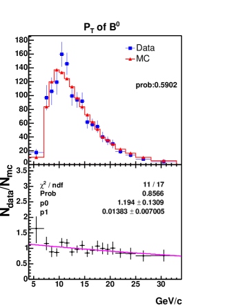
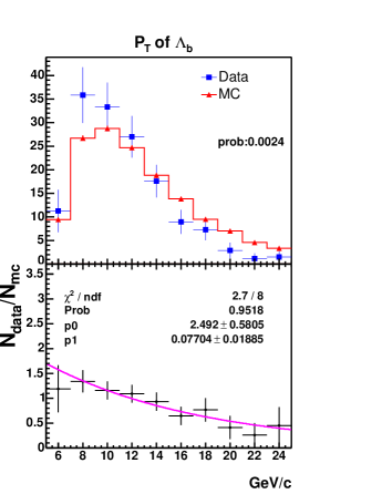
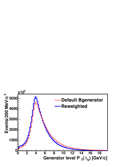
Figure 6.1: Comparison of reconstructed $B^{0}$ (left) and $\Lambda_{b}$ (right) $P_{T}$ spectrum between data and Bgenerator (MC). The top figures show the $P_{T}$ distribution while the bottom figures show the ratio data/MC. The curves in the bottom figures are the result of an exponential fit to the ratio. It is evident that the MC $P_{T}$ spectrum is harder than that of the data.

Figure 6.2: Generator level $\Lambda_{b}$ $P_{T}$ spectra before and after the reweighting.

Table 6.1: Simulated Runs in the MC sample.

Range	Run	$\int{\cal L}\;dt$ ($\mathrm{pb^{-1}}$)	Comment
138809–143000	140129	3.4	Scenario A implemented
143001–146000	145005	4.0	Tevatron incident
146001–149659	148824	4.2	SVX coverage improved
	149387	2.9
149660–150009	149663	0.6	SVT optimization (coverage+patterns)
150010–152668	150820	4.1	$L_{xy}$ $>$ 200 $\mu$m cut added
	151844	3.7
	152520	3.5
152669–156487	152967	3.6	XFT from 2-miss to 1-miss
	153327	3.7
	153447	3.7
	153694	2.4
	154452	4.2
	154654	4.9
	155364	4.3
	155795	2.5
	155895	3.6
	156116	3.7
	156484	2.6
159603–164302	160230	3.7	data taken after the shutdown
	160441	3.4
	160823	3.7
	161029	3.8
	161379	3.3
	161678	3.9
	162130	3.6
	162393	3.6
	162498	5.6
	162631	5.7
	162857	4.4
	163064	3.7
	163431	4.3
164303–167715	164451	4.6	SVT change from 4/4 to 4/5
	164844	3.5
	165121	2.9
	165271	3.9
	165412	3.6
	166008	6.0
	166063	2.9
	166567	5.2
	166662	5.3
	167053	5.9
	167186	2.2
	167506	4.0
	167551	2.7
Total		170.9

6.2 Monte Carlo and Data Comparison

To confirm that the simulation accurately reproduces the data, we compare various reconstructed distributions from the MC with the same distribution from the data. To ensure a fair comparison, the combinatorial background present in the signal region of data has to be removed . We perform a sideband subtraction for the $\overline{B}^{0}\rightarrow D^{*+}\pi^{-}$, $\overline{B}\rightarrow D^{*+}\mu^{-}X$, $\overline{B}^{0}\rightarrow D^{+}\pi^{-}$ and $\overline{B}\rightarrow D^{+}\mu^{-}X$ decays. For the $\Lambda_{b}\rightarrow\Lambda_{c}^{+}\pi^{-}$ and $\overline{B}\rightarrow\Lambda_{c}^{+}\mu^{-}X$ decays, a sideband subtraction can not remove all the backgrounds in the signal region as explained later in the text and in Section 5.2. Instead, a signal distribution of variable “X” is obtained by fitting $M_{\Lambda_{c}\pi}$ and $M_{pK\pi}$ to get the number of signal events in bins of variable “X”. For all the semileptonic modes, we include the MC samples of the physics backgrounds described in Section 7.2. The distribution from each physics background is scaled according to the assumed or measured branching ratio for that background. In addition, the distribution of each compared variable from the fake muons is subtracted from the data. The distribution from the fake muons is obtained by reconstructing the “fake muon-charm” final state as described in Section 7.3. The combinatorial background in the “fake muon-charm” is removed using the same method as described above for the real muon. See Figure 6.3 for the $M_{D\mu}$ from the muon fakes.

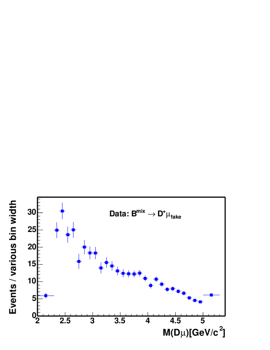
Figure 6.3: $M_{D\mu}$ from the $B\rightarrow D^{+}\mu_{fake}$ data. The distribution is sideband subtracted using $M_{K\pi\pi}$.

For the $B$ meson semileptonic channels, the mass difference between $D^{*+}$ and $D^{0}$ in the $\overline{B}\rightarrow D^{*+}\mu^{-}X$ mode ($M_{K\pi\pi}$ - $M_{K\pi}$), and mass of $D^{+}$ in the $\overline{B}\rightarrow D^{+}\mu^{-}X$ mode ($M_{K\pi\pi}$), are used as the variables to perform the sideband subtraction. The signal region for both these modes is defined as:

$$|M-M_{\mathrm{PDG}}|<2\sigma,$$ (6.4)

and the sideband region is defined as:

$$4\sigma<|M-M_{\mathrm{PDG}}|<6\sigma.$$ (6.5)

The background function is assumed to be a straight line. Therefore, the amount of background in our signal region is the same as that in our sideband regions. We obtain a clean signal distribution by subtracting the histogram in the sideband region from the histogram in the signal region. Figure 6.4 displays the signal and sideband regions of $M_{K\pi\pi}$ - $M_{K\pi}$ and $M_{K\pi\pi}$.

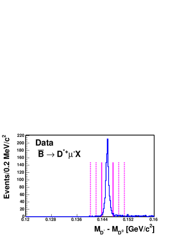
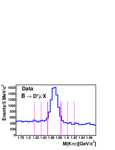
Figure 6.4: Invariant mass difference $M_{K\pi\pi}-M_{K\pi}$ (left) and invariant mass $M_{K\pi\pi}$ (right) showing our reconstructed $\overline{B}\rightarrow D^{*+}\mu^{-}X$ and $\overline{B}\rightarrow D^{+}\mu^{-}X$ signals. The vertical solid (dashed) lines indicate the signal (sideband) regions.

For the $B$ meson hadronic modes, we use the upper mass sideband above the signal peak to perform the sideband subtraction. The lower mass region below the signal peak consists of both combinatorial background and partially reconstructed $B$ decays. However, the background in the signal region and in the upper mass region above the peak is mainly combinatorial as shown in Figures 5.11 – 5.13. We have learned in Section 5.2 that the combinatorial background is adequately described by an exponential function. Therefore, we fit the upper mass region to an exponential function. We further extrapolate the exponential to the signal region and obtain the ratio of the background in our signal region to that in our upper mass sideband, $R_{\mathrm{bg}}$. The histogram of the compared variable extracted from the upper mass sideband is scaled by $R_{\mathrm{bg}}$ and subtracted from the histogram in the signal region. See Figure 6.5 for the $B^{0}$ mass signal region we define and the upper mass region we fit to an exponential.

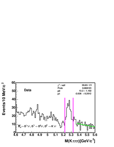
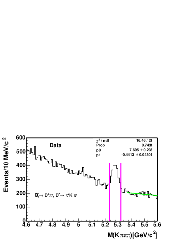
Figure 6.5: Invariant mass $M_{K\pi\pi\pi}$ for $\overline{B}^{0}\rightarrow D^{*+}\pi^{-}$ (top) and $\overline{B}^{0}\rightarrow D^{+}\pi^{-}$ (bottom) signals. The vertical solid lines indicate the signal region. The upper mass regions on the right are fitted to exponential functions.

For the $\overline{B}\rightarrow\Lambda_{c}^{+}\mu^{-}X$ and $\Lambda_{b}\rightarrow\Lambda_{c}^{+}\pi^{-}$ modes, there are non-negligible backgrounds under the signal peak from the reflections due to a mis-assignment of the mass for one of the particles, see Chapter 5 for more details. This type of background has a different behavior from the combinatorial background in the sideband region. Since a background-free sideband subtraction is difficult to perform, we choose to fit the number of signal events in each bin of the variables which we want to compare. For the number of $\overline{B}\rightarrow\Lambda_{c}^{+}\mu^{-}X$ candidates, the $M_{pK\pi}$ distribution is fitted to a signal Gaussian and a second-order polynomial background as shown in Figure 6.6. For the number of $\Lambda_{b}\rightarrow\Lambda_{c}^{+}\pi^{-}$candidates, the $M_{pK\pi\pi}$ distribution is fitted to a simplified model: a Gaussian signal and an exponential background, as shown in Figure 6.7. Note that although the $\Lambda_{b}$ fit model is simplified, the systematic uncertainty due to the naive model is no more than $3\%$ of the number of signal events in each bin compared with the $15\%$ statistical uncertainty. The widths of $M_{pK\pi}$ and $M_{K\pi}$ are fixed to the values obtained from the full statistics when doing the fit. Figure 6.9 shows the data and MC comparison using the fit values obtained from Figures 6.6– 6.7.

When comparing the MC and data distributions, if the number of data signal events in one bin is less than 20, that bin is combined with the next bin until the sum of the events is over 20. Then a $\chi^{2}$ is computed,

$$\chi^{2}=\sum_{i}^{n}\frac{(N_{{\mathrm{M}C}}(i)-N_{{\mathrm{d}ata}}(i))^{2}}{\sigma_{{\mathrm{M}C}}(i)^{2}+\sigma_{{\mathrm{d}ata}}(i)^{2}}$$ (6.6)

where $i$ stands for $i^{th}$ bin and total number of bins in a histogram is $n$. The number of degree freedom is $n-1$. For the $\overline{B}\rightarrow\Lambda_{c}^{+}\mu^{-}X$ and $\Lambda_{b}\rightarrow\Lambda_{c}^{+}\pi^{-}$ modes, a $\chi^{2}$ is also calculated except that the bin width of each variable is fixed in this case. Besides the $\chi^{2}$ test, we also plot the ratio data/MC. We fit the ratio to a first-order polynomial and check if the slope, ${\cal M}$, is consistent with zero.

In the first pass, we find discrepancies in the $P_{T}$ spectra of $B^{0}$ and $\Lambda_{b}$ between MC and data (see Figure 6.2). As the semileptonic modes are three-body decays and the hadronic modes are two-body decays, the efficiency of the trigger and analysis $P_{T}$ cut depends strongly on the $P_{T}$ of $B$ hadron (see Figure 6.9). We decide to reweight the $P_{T}$ spectra of $B^{0}$ and $\Lambda_{b}$ as described in Section 6.1. Figures 6.10– 6.11 show the comparison between MC and data for the analysis cut variables of the $\Lambda_{b}\rightarrow\Lambda_{c}$ modes. Figure 6.12 shows the comparison for the $M_{D^{*}\mu}$, $M_{D\mu}$, and the $M_{\Lambda_{c}\mu}$ from the phase space MC before and after multiplying each bin entry with a scaling factor. The scaling factor is obtained by dividing the $M_{\Lambda_{c}\mu}$ distribution from the form factor weighted (see Section 6.3) by that from the phase space generator-level MC. The agreement of the MC $M_{\Lambda_{c}\mu}$ distribution with that from the data has significantly improved after applying the scaling factor. In addition, we compare the efficiency of the $M_{\Lambda_{c}\mu}$ cut in the MC and data, given that the other (N-1) analysis cuts are applied. The contribution of the fake muons and physics backgrounds are included. Since there are uncertainties from the fit to both data and MC, the efficiency is defined as:

$$\epsilon=\frac{n}{N},$$ (6.7)

where $n$ is the number of events after making all the analysis cuts and $N$ is the number of events after making the $N-1$ cuts. The uncertainty on the efficiency is derived by Heinrich [77]:

$$\sigma_{\epsilon}=\sqrt{(\epsilon\cdot\frac{\sigma_{N}}{N})^{2}+(1-2\epsilon)\cdot(\frac{\sigma_{n}}{N})^{2}},$$ (6.8)

where $\sigma_{N}$ and $\sigma_{n}$ are the uncertainties from the fit. We find the data give an efficiency of 0.77$\pm$0.04, while the form factor weighted MC gives an efficiency of 0.72$\pm$0.05, which is in good agreement with the data efficiency. Other distributions important for this analysis may be found in Yu[65].

In general, the MC describes the data well except for the pseudo $c\tau$ of $\Lambda_{c}\mu$, and the $\chi^{2}_{r-\phi}$ of the $B$ and charm vertex fits. For the disagreement in the vertex fit $\chi^{2}_{r-\phi}$, as it is beyond the scope of this analysis to scale the measurement errors in the MC, we choose to make a loose cuts on the data $\chi^{2}_{r-\phi}$. In Section 8.1.3, we perform a cross-check of the relative branching ratio variation by dividing the data into two subsets, according to the cuts on the pseudo $c\tau$ of $\Lambda_{c}\mu$, $\chi^{2}_{r-\phi}$ and other variables. We do not see significant inconsistency. Therefore, we do not assign any systematic uncertainties for these variables.

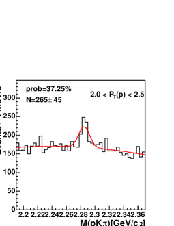
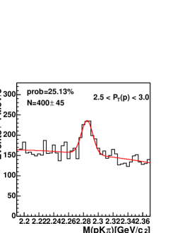
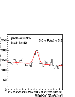
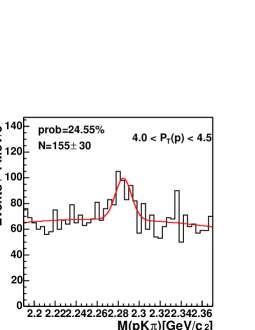
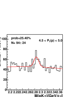
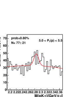
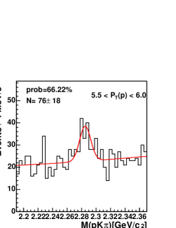
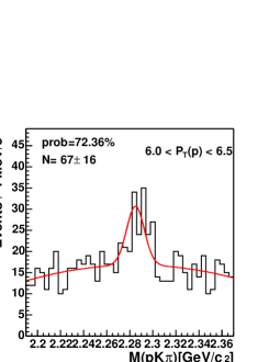
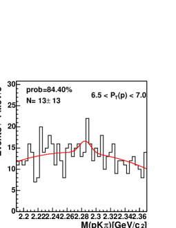
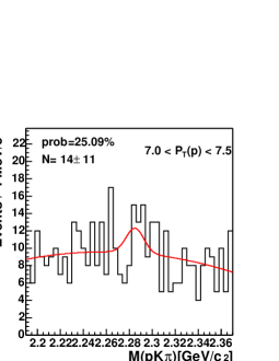
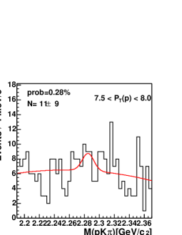
Figure 6.6: Example of $\Lambda_{c}^{+}$ mass fit for the MC and data comparison. The variable to compare is the $P_{T}$ of proton, from 2 to 8 $\rm GeV/c$, in bins of 0.5 $\rm GeV/c$. $M_{pK\pi}$ is fitted to a signal Gaussian and a second-order polynomial.

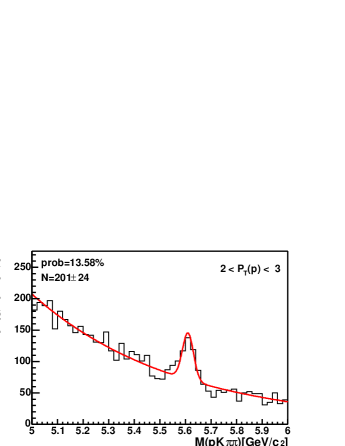
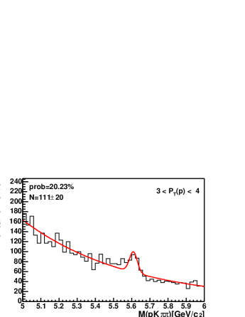
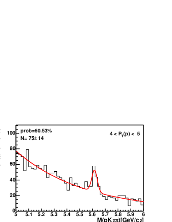
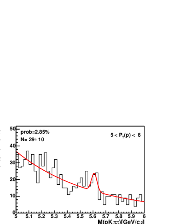
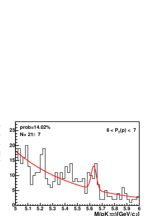
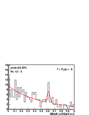
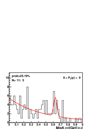
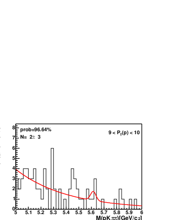
Figure 6.7: Example of $\Lambda_{b}$ mass fit for the MC and data comparison. The variable to compare is the $P_{T}$ of proton, from 2 to 10 $\rm GeV/c$, in bins of 1 $\rm GeV/c$. $M_{pK\pi\pi}$ is fitted to a signal Gaussian and an exponential background.

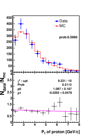
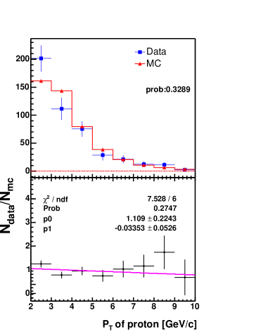
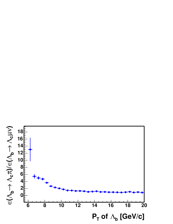
Figure 6.8: MC and data comparison of $P_{T}$(proton). The data points come from the fit to $M_{pK\pi}$ in Figure 6.6 (left) and the fit to $M_{pK\pi\pi}$ in Figure 6.7 (right).

Figure 6.9: MC Efficiency ratio of $\Lambda_{b}\rightarrow\Lambda_{c}^{+}\pi^{-}$ to $\Lambda_{b}\rightarrow\Lambda_{c}^{+}\mu^{-}\overline{\nu}_{\mu}$ as a function of the transverse momentum of $\Lambda_{b}$.

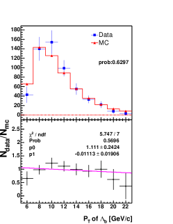
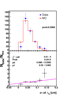
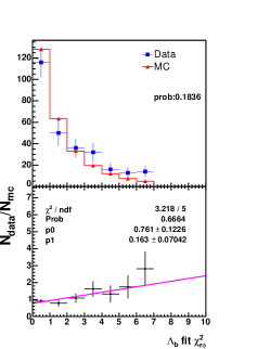
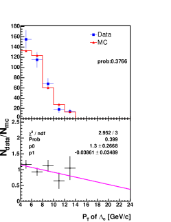
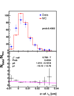
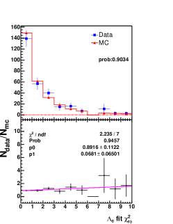
Figure 6.10: $\Lambda_{b}\rightarrow\Lambda_{c}^{+}\pi^{-}$ MC and data comparison: from the top left to the bottom right are: $P_{T}$($\Lambda_{b}$), $c\tau$($\Lambda_{b}$), vertex fit $\chi^{2}_{r-\phi}$ for the $\Lambda_{b}$ vertex, $P_{T}$($\Lambda_{c}^{+}$), $c\tau$($\Lambda_{c}^{+}$), and vertex fit $\chi^{2}_{r-\phi}$ for the $\Lambda_{c}^{+}$ vertex.

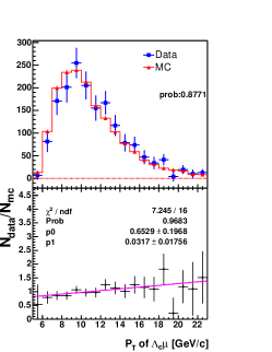
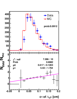
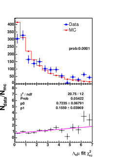
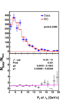
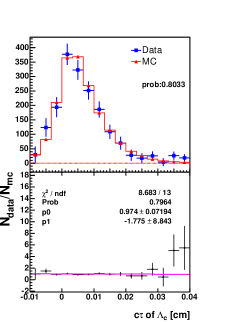
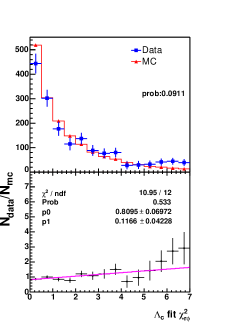
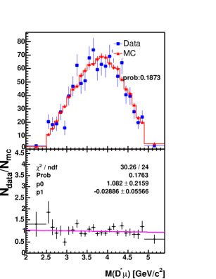
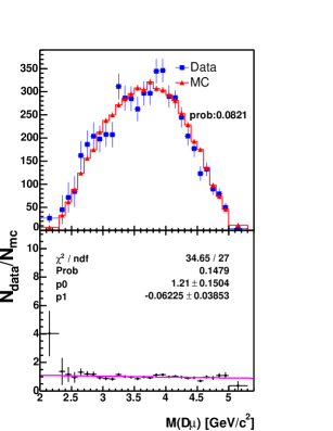
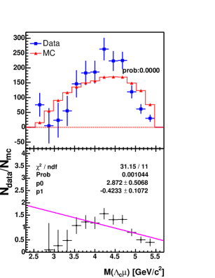
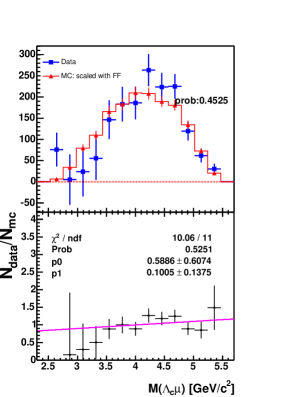
Figure 6.11: $\overline{B}\rightarrow\Lambda_{c}^{+}\mu^{-}X$ MC and data comparison: from the top left to the bottom right are: $P_{T}$($\Lambda_{c}\mu$), $c\tau$($\Lambda_{c}\mu$), vertex fit $\chi^{2}_{r-\phi}$ for the $\Lambda_{c}\mu$ vertex, $P_{T}$($\Lambda_{c}^{+}$), $c\tau$($\Lambda_{c}^{+}$), and vertex fit $\chi^{2}_{r-\phi}$ for the $\Lambda_{c}^{+}$ vertex.

Figure 6.12: four track invariant mass MC and data comparison: from the top left to the bottom right are: $M_{D^{*}\mu}$, $M_{D\mu}$, $M_{\Lambda_{c}\mu}$ (phase space MC without scaling), $M_{\Lambda_{c}\mu}$ (phase space MC after scaling).

6.3 Acceptance, Trigger and Reconstruction Efficiencies of Signal

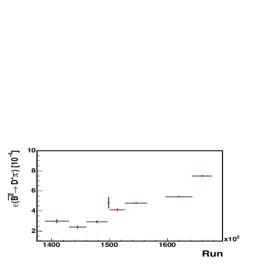
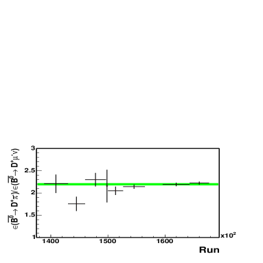
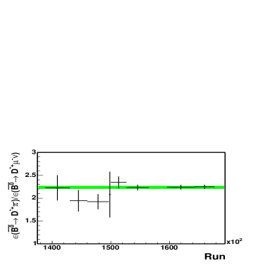
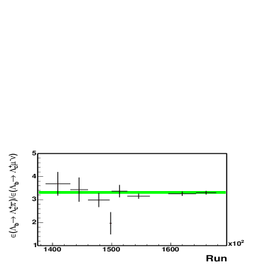
Figure 6.13: $\overline{B}^{0}\rightarrow D^{+}\pi^{-}$ MC total efficiency (left) and the ratio of that to the $\overline{B}^{0}\rightarrow D^{+}\mu^{-}\overline{\nu}_{\mu}$ MC efficiency (right) in eight different hardware configurations. The shaded area represents the average efficiency ratio including the uncertainty.

Figure 6.14: Total efficiency ratio of $\overline{B}^{0}\rightarrow D^{*+}\pi^{-}$ to $\overline{B}^{0}\rightarrow D^{*+}\mu^{-}\overline{\nu}_{\mu}$ (left) and $\Lambda_{b}\rightarrow\Lambda_{c}^{+}\pi^{-}$ to $\Lambda_{b}\rightarrow\Lambda_{c}^{+}\mu^{-}\overline{\nu}_{\mu}$ (right) MC in eight different hardware configurations. The shaded area represents the total average efficiency ratio including the uncertainty.

We obtain the product of the acceptance, trigger and reconstruction efficiencies using the MC described in Section 6.1. The total efficiency is defined as: the number of reconstructed events surviving the trigger simulation and analysis cuts, divided by the total number of events generated. Efficiencies for the backgrounds are found in Chapter 7. Our data could be divided into eight sub-periods under different trigger and hardware configurations, see Table 6.1. In this analysis, because the final states are nearly alike, we expect that the ratio of the efficiencies to be independent of the detector, trigger and calibration effects. To confirm this, we divide our signal MC samples into eight sub-periods and calculate their efficiencies and the ratio of hadronic to semileptonic modes. Tables 6.4– 6.4 list the efficiencies for our signals. Figure 6.14–6.14 show that the absolute efficiency may vary dramatically in each period, however the efficiency ratio of the hadronic to the semileptonic mode is quite stable.

Note that because Bloom and Dagenhart [78] find a difference in the CMU muon reconstruction efficiency between MC and data, we apply a scaling factor on the efficiencies of the semileptonic signals and backgrounds: $R=0.986\pm 0.003.$ In addition, Giagu, Herndon and Rescigno [79][80] notice that there are differences in the XFT efficiencies for the charged kaons, pions, and protons, when the XFT configuration is switched to the “1-miss” mode, i.e. when the tracking algorithm in the XFT requires at least 11 hits of 12 wires from each COT axial superlayer. The COT frond-end electronics requires a minimum input charge from the ionization of the incident particle. At a fixed momentum, protons and kaons deposit less charge than the pions, have more hits below the electronics threshold, and fail the stringent XFT “1-miss” requirement. Therefore, in general, the proton and kaon XFT efficiencies are lower than that of the pion. Figure 6.15(top) shows that kaon and pion XFT efficiencies are identical in the MC and need to be corrected. Giagu, Herndon and Rescigno measure the ratio, data/MC for the XFT efficiencies of pions, kaons and protons, as shown in Figure 6.15. We reweight the MC events numerically according to the ratio:

$$C_{\pi} = 1.002-\frac{0.067}{P_{T}},$$

$$C_{K} = 0.969-\frac{0.094}{P_{T}},$$

$$C_{p} = 1.06-\frac{1.3}{P_{T}}+\frac{3.2}{P_{T}^{2}}-\frac{2.2}{P_{T}^{3}},$$

where $P_{T}$ is the transverse momentum of the track that passes the trigger cuts in our reconstruction program.

Finally, one additional scaling factor has to be applied on all the $\Lambda_{b}$ decays with $\Lambda_{c}\mu$ in the final state. We have mentioned in Section 6.1 that a phase space decay model was used for these decays. In a phase space, the event density in the $w$-$\cos\theta$ plane is a constant within the kinematic boundary. The $w$ is the scalar product of the $\Lambda_{b}$ and $\Lambda_{c}$ four-velocities, and $\theta$ is the angle between the muon and the neutrino momentum vectors in the $\Lambda_{b}$ rest frame. The form factors that describe the strong interaction in the $\Lambda_{b}$ semileptonic decay modify the event distribution in the phase space and change the fraction of events accepted. We obtain the scaling factor in the following way: Using the “acceptance-rejection” method, we reweight the generator-level $\Lambda_{b}\rightarrow\Lambda_{c}^{+}\mu^{-}\overline{\nu}_{\mu}$ MC according to:

$$f_{c}=\frac{d\Gamma(\Lambda_{b}\rightarrow\Lambda_{c}^{+}\mu^{-}\overline{\nu}_{\mu})}{dw}\cdot\frac{T(\cos\theta,w)}{P(w)},$$ (6.9)

where the differential semileptonic decay rate, $\frac{d\Gamma(\Lambda_{b}\rightarrow\Lambda_{c}^{+}\mu^{-}\overline{\nu}_{\mu})}{dw}$, is obtained from Huang[36]. The $T(\cos\theta,w)$ includes the $W$ spin effect and describes the correlation between the $\mu$ and $\overline{\nu}_{\mu}$, and

$$P(w)=\int_{{\cos\theta}_{\mathrm{min}}(w)}^{{\cos\theta}_{\mathrm{max}}(w)}T(\cos\theta,w)d\cos\theta.$$ (6.10)

Here, ${\cos\theta}_{\mathrm{max}}$ and ${\cos\theta}_{\mathrm{min}}$ specify the kinematic range and are functions of $w$. Figure 6.16 shows the phase space and the $w$ distribution from the phase space and the form factor reweighted MC. Then, we apply generator-level analysis cuts to obtain the acceptance. We further divide this acceptance by that from the phase space MC and obtain a scaling factor of 0.994$\pm$0.025, where the uncertainty is dominated by the size of the MC sample.

Table 6.2: Total efficiency and ratios for $\overline{B}^{0}\rightarrow D^{*+}\pi^{-}$ and $\overline{B}^{0}\rightarrow D^{*+}\mu^{-}\overline{\nu}_{\mu}$.

Run Range	$\int{\cal L}\;dt$	$\epsilon_{\overline{B}^{0}\rightarrow D^{*+}\pi^{-}}$	$\epsilon_{\overline{B}^{0}\rightarrow D^{*+}\mu^{-}\overline{\nu}_{\mu}}$	$\epsilon$ Ratio
	($\mathrm{pb^{-1}}$)	($10^{-4}$)	($10^{-4}$)
138809–143000	3.4	1.72 $\pm$ 0.15	0.77 $\pm$ 0.07	2.22 $\pm$ 0.28
143001–146000	4.0	1.42 $\pm$ 0.12	0.73 $\pm$ 0.06	1.94 $\pm$ 0.24
146001–149659	7.1	1.57 $\pm$ 0.10	0.82 $\pm$ 0.05	1.92 $\pm$ 0.17
149660–150009	0.6	2.35 $\pm$ 0.40	1.13 $\pm$ 0.19	2.08 $\pm$ 0.50
150010–152668	11.3	2.65 $\pm$ 0.10	1.13 $\pm$ 0.05	2.34 $\pm$ 0.13
152669–156487	39.2	2.74 $\pm$ 0.06	1.23 $\pm$ 0.03	2.23 $\pm$ 0.07
159603–164302	52.7	3.10 $\pm$ 0.05	1.38 $\pm$ 0.02	2.24 $\pm$ 0.05
164303–167715	52.7	4.27 $\pm$ 0.06	1.90 $\pm$ 0.03	2.25 $\pm$ 0.05
Total average	171.0	3.22 $\pm$ 0.03	1.44 $\pm$ 0.01	2.24 $\pm$ 0.03

Table 6.3: Total efficiency and ratios for $\overline{B}^{0}\rightarrow D^{+}\pi^{-}$ and $\overline{B}^{0}\rightarrow D^{+}\mu^{-}\overline{\nu}_{\mu}$.

Run Range	$\int{\cal L}\;dt$	$\epsilon_{\overline{B}^{0}\rightarrow D^{+}\pi^{-}}$	$\epsilon_{\overline{B}^{0}\rightarrow D^{+}\mu^{-}\overline{\nu}_{\mu}}$	$\epsilon$ Ratio
	($\mathrm{pb^{-1}}$)	($10^{-4}$)	($10^{-4}$)
138809–143000	3.4	2.99 $\pm$ 0.19	1.35 $\pm$ 0.09	2.21 $\pm$ 0.21
143001–146000	4.0	2.39 $\pm$ 0.16	1.36 $\pm$ 0.09	1.76 $\pm$ 0.16
146001–149659	7.1	2.93 $\pm$ 0.13	1.28 $\pm$ 0.06	2.30 $\pm$ 0.15
149660–150009	0.6	4.82 $\pm$ 0.57	2.23 $\pm$ 0.27	2.16 $\pm$ 0.37
150010–152668	11.3	4.12 $\pm$ 0.14	2.01 $\pm$ 0.06	2.05 $\pm$ 0.09
152669–156487	39.2	4.79 $\pm$ 0.08	2.24 $\pm$ 0.04	2.14 $\pm$ 0.05
159603–164302	52.7	5.43 $\pm$ 0.07	2.48 $\pm$ 0.03	2.19 $\pm$ 0.04
164303–167715	52.7	7.49 $\pm$ 0.08	3.37 $\pm$ 0.04	2.22 $\pm$ 0.03
Total average	171.0	5.67 $\pm$ 0.04	2.58 $\pm$ 0.02	2.20 $\pm$ 0.02

Table 6.4: Total efficiency and ratios for $\Lambda_{b}\rightarrow\Lambda_{c}^{+}\pi^{-}$ and $\Lambda_{b}\rightarrow\Lambda_{c}^{+}\mu^{-}\overline{\nu}_{\mu}$.

Run Range	$\int{\cal L}\;dt$	$\epsilon_{\Lambda_{b}\rightarrow\Lambda_{c}^{+}\pi^{-}}$	$\epsilon_{\Lambda_{b}\rightarrow\Lambda_{c}^{+}\mu^{-}\overline{\nu}_{\mu}}$	$\epsilon$ Ratio
	($\mathrm{pb^{-1}}$)	($10^{-4}$)	($10^{-4}$)
138809–143000	3.4	1.84 $\pm$ 0.15	0.50 $\pm$ 0.06	3.69 $\pm$ 0.51
143001–146000	4.0	1.23 $\pm$ 0.12	0.36 $\pm$ 0.04	3.43 $\pm$ 0.53
146001–149659	7.1	1.42 $\pm$ 0.09	0.48 $\pm$ 0.04	2.98 $\pm$ 0.30
149660–150009	0.6	2.23 $\pm$ 0.39	1.13 $\pm$ 0.19	1.98 $\pm$ 0.48
150010–152668	11.3	2.13 $\pm$ 0.12	0.63 $\pm$ 0.04	3.37 $\pm$ 0.27
152669–156487	39.2	2.37 $\pm$ 0.05	0.75 $\pm$ 0.02	3.15 $\pm$ 0.11
159603–164302	52.7	2.67 $\pm$ 0.05	0.82 $\pm$ 0.02	3.26 $\pm$ 0.09
164303–167715	52.7	3.76 $\pm$ 0.06	1.14 $\pm$ 0.02	3.30 $\pm$ 0.08
Total average	171.0	2.86 $\pm$ 0.03	0.86 $\pm$ 0.01	3.31 $\pm$ 0.05

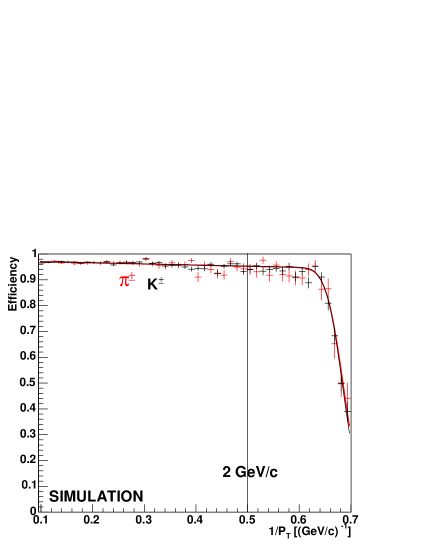
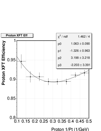
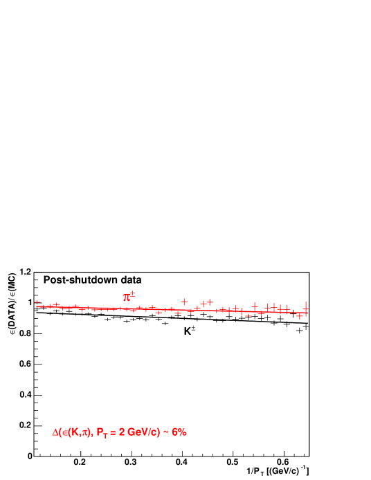
Figure 6.15: Giagu and Rescigno [79] find that $K$ and $\pi$ XFT efficiencies in the MC (top left) are identical. The relative proton (top right) and $K$, $\pi$ (bottom) XFT efficiencies between MC and data, in bins of 1/$P_{T}$, are fit to a third order polynomial by Herndon [80], and to a first order polynomial by Giagu and Rescigno [79], respectively.

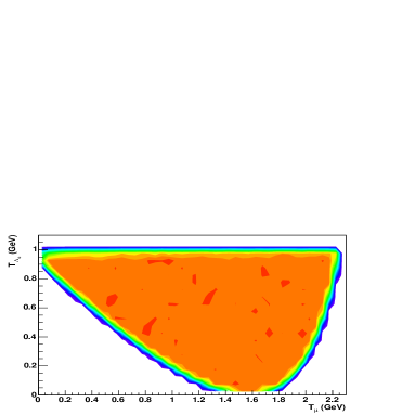
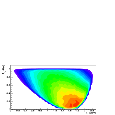
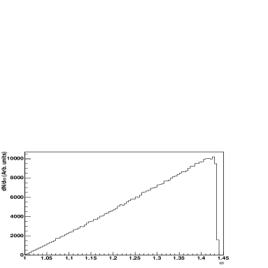
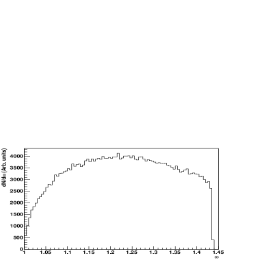
Figure 6.16: The phase space (top) and the $w$ (bottom) distribution obtained from the $\Lambda_{b}\rightarrow\Lambda_{c}^{+}\mu^{-}\overline{\nu}_{\mu}$ phase space MC, before (left) and after (right) reweighting the events according to the semileptonic form factors from Huang[36].

6.4 Summary

We have described the procedure of generating MC samples and compared the MC distributions with those in the data. In general, the MC and data are in good agreement. We also obtain the signal efficiencies from the MC. It is confirmed that the efficiency ratios from both the $\Lambda_{b}$ and $B^{0}$ modes are insensitive to the time variation of beam lines and SVT trigger configurations.

Chapter 7 Backgrounds of the Semileptonic Modes

Unlike the $e^{+}e^{-}$ collider experiments, BELLE [24] and BABAR [25], the initial energies of the $B$ hadrons are unknown in CDF. For the hadronic channels, such as $\overline{B}^{0}\rightarrow D^{+}\pi^{-}$, the $B$ meson is fully reconstructed using the momenta of the daughter particles ($D^{+}$ and $\pi^{-}$) at the point of the parent decay. However, for the semileptonic channels, such as $\overline{B}^{0}\rightarrow D^{+}\mu^{-}\overline{\nu}_{\mu}$, without the information of initial energies, it is difficult to constrain the momenta of the missing neutrinos and fully reconstruct the $B$ candidates. Therefore, the $D^{*}\mu$, $D\mu$ and $\Lambda_{c}\mu$ combinations we observe in the data consist of the exclusive semileptonic signals, $\overline{B}^{0}\rightarrow D^{*+}\mu^{-}\overline{\nu}_{\mu}$, $\overline{B}^{0}\rightarrow D^{+}\mu^{-}\overline{\nu}_{\mu}$, $\Lambda_{b}\rightarrow\Lambda_{c}^{+}\mu^{-}\overline{\nu}_{\mu}$, in the presence of other backgrounds. These backgrounds arise from three sources:

• physics backgrounds: $B$ hadron decays into similar final states, a charm hadron, a real muon and other tracks.

• muon fakes: a charm hadron and a track which fakes a muon.

• $b\overline{b}$ and $c\overline{c}$: two $B$ or charm hadrons from the $b\overline{b}$ and $c\overline{c}$ pairs decay into a $D^{*+}$ ($D^{+}$, $\Lambda_{c}^{+}$) and a muon, respectively.

The goal is to measure the relative partial decay widths of the exclusive semileptonic decays to hadronic decays. The backgrounds listed above should be subtracted from the observed inclusive semileptonic signal in the data. The ratio of branching fractions is then calculated as follows:

$$\frac{{\cal B}_{\mathrm{semi}}}{{\cal B}_{\mathrm{had}}}=(\frac{N_{\mathrm{inclusive\;semi}}-N_{\mathrm{physics}}-N_{\mathrm{fake\mu}}-N_{c\overline{c},\;b\overline{b}}}{N_{\mathrm{had}}})\cdot\frac{\epsilon_{\mathrm{had}}}{\epsilon_{\mathrm{semi}}},$$ (7.1)

where ${\cal B}$ stands for the branching ratio, $\epsilon$ is the efficiency from the MC. We estimate the contribution from the physics and $b\overline{b}$, $c\overline{c}$ backgrounds, using the efficiencies from the MC and the branching ratios from the Particle Data Group (PDG) [8]. We normalize the backgrounds to the observed number of events in the fully reconstructed hadronic signal in the data,

$$N_{\mathrm{physics}\;(b\overline{b},c\overline{c})}=N_{\mathrm{had}}\cdot\sum\frac{{\cal B}_{i}\cdot\epsilon_{i}}{{\cal B}_{\mathrm{had}}\cdot\epsilon_{\mathrm{had}}}.$$ (7.2)

Substituting Equation 7.2 into Equation 7.1, $N_{\mathrm{had}}$ cancels. The estimate of $b\overline{b}$, $c\overline{c}$ and physics background contributions is then free from the uncertainties in the hadronic yields. In the case of fake muons, we subtract the fake muon candidates measured in the data directly.

The branching ratios of $B^{0}$ hadronic modes in Equation 7.2 come from the world average in the PDG. For the $\Lambda_{b}$ mode, we extract ${\cal B}(\Lambda_{b}\rightarrow\Lambda_{c}^{+}\pi^{-})$ from the recent CDF result, $\frac{\sigma_{\Lambda_{b}}(P_{T}>6.0){\cal B}(\Lambda_{b}\rightarrow\Lambda_{c}^{+}\pi^{-})}{\sigma_{B^{0}}(P_{T}>6.0){\cal B}(\overline{B}^{0}\rightarrow D^{+}\pi^{-})}$ by Le, et al. [68]. Because Le’s measurement requires the ratio of the $\Lambda_{b}$ to $B^{0}$ production cross sections as an input, we correct for the ratio in Section 7.1 and obtain ${\cal B}(\Lambda_{b}\rightarrow\Lambda_{c}^{+}\pi^{-})$. Sections 7.2– 7.4 estimate the amount of backgrounds in the semileptonic signal. We will show that the dominant signal contamination is from the physics background. The second largest background arises from muon fakes. The smallest background source is from $b\overline{b}$ and $c\overline{c}$.

7.1 Correction of $\frac{\sigma_{\Lambda_{b}}}{\sigma_{B^{0}}}$ and ${\cal B}(\Lambda_{b}\rightarrow\Lambda_{c}^{+}\pi^{-})$

CDF has made a number of measurements of the relating information from the decay of $B$-hadron to that of another with similar topology, such as

$\frac{\sigma_{\Lambda_{b}}(P_{T}>6.0){\cal B}(\Lambda_{b}\rightarrow\Lambda_{c}^{+}\pi^{-})}{\sigma_{B^{0}}(P_{T}>6.0){\cal B}(\overline{B}^{0}\rightarrow D^{+}\pi^{-})}$ [68] or $\frac{\sigma_{\Lambda_{b}}(P_{T}>4.0){\cal B}(\Lambda_{b}\rightarrow J/\psi\Lambda)}{\sigma_{B^{0}}(P_{T}>4.0){\cal B}(B^{0}\rightarrow J/\psi K_{s}^{0})}$ [81].

In order to extract the individual branching fraction, one must have the knowledge of the production cross section. Since no production cross section measurements exist for $\Lambda_{b}$, one must infer the cross-section using other means. Using the total $b$-quark cross-section [41], the fragmentation fraction ($f_{u}$, $f_{d}$, $f_{s}$ and $f_{\mathrm{baryon}}$), and assuming the composition of the $b$-baryons is dominated by $\Lambda_{b}$, i.e. $f_{\Lambda_{b}}\cong f_{\mathrm{baryon}}$, we may infer the production cross-section of any $B$-hadron species. However, the fragmentation fractions assume the entire $P_{T}$ spectrum is measured for both the particles ($B^{0}$ and $\Lambda_{b}$) in the above ratios. If the $P_{T}$ spectrum is incorrect, the kinematic acceptance used in the above ratios will be over- or under-estimated. In addition, since most analyses at CDF require a $P_{T}$ threshold to improve the signal to background ratio, any difference in the $P_{T}$ spectrum between the particles participating in the ratio will modify the effective fragmentation fraction. Figure 7.1 illustrates this effect for a very small difference in the spectrum (top) and a large difference in the spectrum (bottom). In this section, we derive corrections for the production cross sections $\frac{\sigma_{\Lambda_{b}}}{\sigma_{B^{0}}}$ to account for their different $P_{T}$ spectra and overestimated kinematic acceptance from the previous measurements.

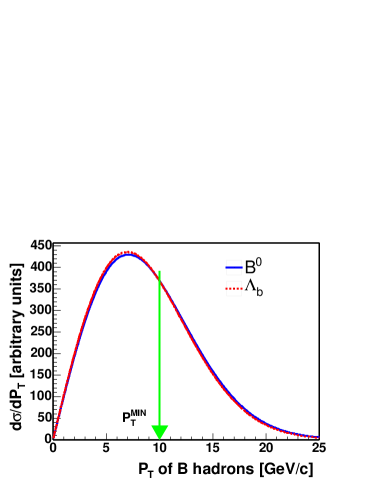
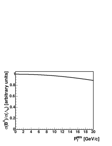
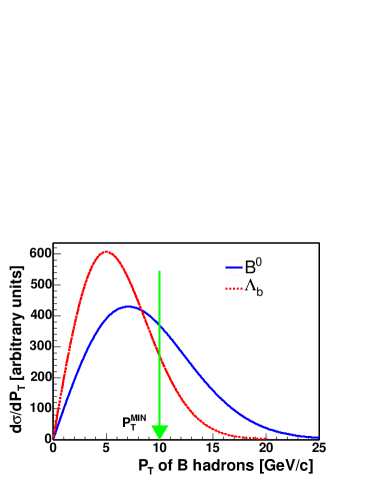
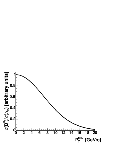
Figure 7.1: $P_{T}$ spectrum of $B^{0}$ and $\Lambda_{b}$ (left) and the dependence of the production ratio on the $P_{T}$ threshold, $P_{T}^{\mathrm{MIN}}$ (right). The top figures show the case where both hadrons have an almost identical spectrum. The ratio of the integrated areas underneath the spectrum, from $P_{T}^{\mathrm{MIN}}$ and above, does not depend much on the value of $P_{T}^{\mathrm{MIN}}$. The bottom figure shows a softer $\Lambda_{b}$ $P_{T}$ spectrum. The ratio of the integrated areas will depend strongly on the value of $P_{T}^{\mathrm{MIN}}$.

To simplify the notation, we define the relative production cross sections of $\Lambda_{b}$ to $B^{0}$ as $\rho$,

$$\rho(x)\equiv\frac{\sigma_{\Lambda_{b}}(P_{T}\ >x\;\rm GeV/c)}{\sigma_{B^{0}}(P_{T}\ >x\;\rm GeV/c)},$$ (7.3)

where $x$ is the $P_{T}$ threshold of the $B$ hadrons in $\rm GeV/c$. When estimating the backgrounds for our semileptonic signals, we choose to use the hadronic signals as the normalization because they are fully reconstructed, and free from indistinguishable physics backgrounds. Efficiencies and branching ratios of the hadronic modes are required when performing the normalization, see Equation 7.2. We use Monte Carlo to calculate the efficiencies and external measurements of hadronic decays for the branching ratios. While precise measurements of ${\cal B}(\overline{B}^{0}\rightarrow D^{*+}\pi^{-})$ and ${\cal B}(\overline{B}^{0}\rightarrow D^{+}\pi^{-})$ exist [8], there is not yet a direct measurement of ${\cal B}(\Lambda_{b}\rightarrow\Lambda_{c}^{+}\pi^{-})$. The CDF Run II measurement of $\rho(6)\times\frac{{\cal B}(\Lambda_{b}\rightarrow\Lambda_{c}^{+}\pi^{-})}{{\cal B}(\overline{B}^{0}\rightarrow D^{+}\pi^{-})}$ by Le, et al. [68] provides an input but requires a good understanding of $\rho(6)$. In addition, we need to know $\rho(4)$ to normalize the $B$ meson background, $B^{0,+}\rightarrow\Lambda_{c}^{+}\mu X$ in the inclusive $\Lambda_{c}\mu$ signal, to $\Lambda_{b}\rightarrow\Lambda_{c}^{+}\pi^{-}$,

$$\frac{N_{B^{0,+}\rightarrow\Lambda_{c}^{+}\mu X}}{N_{\Lambda_{b}\rightarrow\Lambda_{c}^{+}\pi^{-}}}=\frac{1}{\rho(4)}\cdot\frac{{\cal B}_{B^{0,+}\rightarrow\Lambda_{c}^{+}\mu X}\cdot\epsilon_{B^{0,+}\rightarrow\Lambda_{c}^{+}\mu X}}{{\cal B}_{\Lambda_{b}\rightarrow\Lambda_{c}^{+}\pi^{-}}\cdot\epsilon_{\Lambda_{b}\rightarrow\Lambda_{c}^{+}\pi^{-}}}.$$ (7.4)

A lower minimum $P_{T}$ requirement of 4 $\rm GeV/c$ is applied here to cover the entire kinematic range of the B hadron semileptonic decays, see Section 7.2.2 for more details.

The fragmentation fractions $f_{d}$, $f_{u}$, $f_{s}$ and $f_{\mathrm{baryon}}$ in the PDG are defined as the probability for a $b$ quark to hadronize into $B^{0}$, $B^{+}$, $B_{s}^{0}$ or baryons,

$$f_{d} \equiv {\cal B}(\overline{b}\rightarrow B^{0}),$$ (7.5)

$$f_{u} \equiv {\cal B}(\overline{b}\rightarrow B^{+}),$$ (7.6)

$$f_{s} \equiv {\cal B}(\overline{b}\rightarrow B_{s}^{0}),$$ (7.7)

$$f_{\mathrm{baryon}} \equiv {\cal B}(\overline{b}\rightarrow\mathrm{b-baryon}),$$ (7.8)

with the assumption that

$$f_{d}+f_{u}+f_{s}+f_{\mathrm{baryon}}=1.$$ (7.9)

The PDG [82] determines $f_{\mathrm{baryon}}$ by combining the measurements of mean lifetimes, $B^{0}$ mixing parameters and branching ratios by LEP, SLD and Taylor in CDF-I [83]. Nevertheless, it is still questionable whether the $f_{\mathrm{baryon}}$ should be the same for the LEP and the Tevatron experiments. As the collider and the detector environments for Taylor’s analysis are most similar to those for this analysis and we have access to the details of the measurement, we discuss the corrections for Taylor’s $f_{\mathrm{baryon}}/f_{d}$ result, 0.236 $\pm$ 0.084.

Correcting the Kinematic Acceptance

Taylor’s analysis uses electron-charm final states, such as $\overline{B}\rightarrow D^{*+}e^{-}X$, $\overline{B}\rightarrow D^{+}e^{-}X$, and $\overline{B}\rightarrow\Lambda_{c}^{+}e^{-}X$ to measure $f_{\mathrm{baryon}}$. Accurate $\Lambda_{b}$ and $B^{0}$ $P_{T}$ spectra from the fully reconstructed decays were not available at the time. The MC samples [84] in Taylor’s analysis for calculating the acceptance and efficiencies were generated using the default settings in the package Bgenerator as described in Section 6.1. We have shown in Section 6.2 that the $\Lambda_{b}$ and $B^{0}$ $P_{T}$ spectra from the Bgenerator are stiffer than those measured in the data. This leads to an over-estimate of the acceptance and efficiencies, particularly for the $\Lambda_{b}$ decays. One must correct for this effect first.

For technical reasons, it is impossible to repeat a full CDF Run I detector simulation. Consequently, we obtain the correction using generator-level MC. We generate $B^{0}$ and $\Lambda_{b}$ with the default Bgenerator $P_{T}$ spectra as described in Section 6.1. Then we decay $B^{0}$ and $\Lambda_{b}$ using the QQ software package [85] as in Taylor’s analysis. We apply the cuts listed in Table 7.1 on the generator level quantities. These cuts mimic those applied in Taylor’s analysis as much as possible. We divide the number of events which pass the cuts by the number of events with $B^{0}$ ($\Lambda_{b}$) $P_{T}$ $>$ 10 $\rm GeV/c$ and rapidity $|y|$ $<$ 2.0, to obtain the acceptance and efficiencies for the exclusive semileptonic decays: $\overline{B}^{0}\rightarrow D^{+}e^{-}\overline{\nu}_{e}$, and $\Lambda_{b}\rightarrow\Lambda_{c}^{+}e^{-}\overline{\nu}_{e}$. We repeat the same process using the corrected $B^{0}$ and $\Lambda_{b}$ $P_{T}$ spectra as described in Section 6.1, except that we use QQ to decay $\Lambda_{b}$ and $B^{0}$ to be consistent with Taylor’s analysis. The production cross-section ratio derived from the Taylor’s analysis ($\frac{\sigma_{\Lambda_{b}}}{\sigma_{B^{0}}}^{\mathrm{Taylor}}$) could be expressed as a ratio of the number of signal events divided by the ratio of the product of the branching ratio and efficiency for the $\Lambda_{b}\rightarrow\Lambda_{c}^{+}e^{-}\overline{\nu}_{e}$ mode, to the same expression for the $\overline{B}^{0}\rightarrow D^{+}e^{-}\overline{\nu}_{e}$ mode:

$$\frac{\sigma_{\Lambda_{b}}}{\sigma_{B^{0}}}^{\mathrm{Taylor}}=N_{R}\cdot{\cal B}_{R}\cdot\epsilon_{R}^{\mathrm{Taylor}},$$ (7.10)

where we use the following shorthand notation:

$$N_{R} = \frac{N_{\Lambda_{b}\rightarrow\Lambda_{c}^{+}e^{-}\overline{\nu}_{e}}}{N_{\overline{B}^{0}\rightarrow D^{+}e^{-}\overline{\nu}_{e}}},$$ (7.11)

$${\cal B}_{R} = \frac{{\cal B}(\overline{B}^{0}\rightarrow D^{+}e^{-}\overline{\nu}_{e})}{{\cal B}(\Lambda_{b}\rightarrow\Lambda_{c}^{+}e^{-}\overline{\nu}_{e})},$$ (7.12)

$$\epsilon_{R} = \frac{\epsilon_{\overline{B}^{0}\rightarrow D^{+}e^{-}\overline{\nu}_{e}}}{\epsilon_{\Lambda_{b}\rightarrow\Lambda_{c}^{+}e^{-}\overline{\nu}_{e}}}.$$ (7.13)

Using the same notation, we could express the corrected ratio as:

$$\frac{\sigma_{\Lambda_{b}}}{\sigma_{B^{0}}}^{\mathrm{corrected}}=N_{R}\cdot{\cal B}_{R}\cdot\epsilon_{R}^{\mathrm{corrected}}=\frac{\sigma_{\Lambda_{b}}}{\sigma_{B^{0}}}^{\mathrm{Taylor}}\cdot C_{\epsilon}=\frac{f_{d}}{f_{\mathrm{baryon}}}\cdot C_{\epsilon}$$ (7.14)

where

$$C_{\epsilon}=\epsilon_{R}^{\mathrm{corrected}}/\epsilon_{R}^{\mathrm{Taylor}}.$$ (7.15)

This gives us the first correction factor, $C_{\epsilon}$=1.81 $\pm$ 0.04 (stat) ${+0.42\atop-0.22}$ ($P_{T}$). The last uncertainty comes from the uncertainty of the exponential slope used to obtain the corrected $\Lambda_{b}$ $P_{T}$ spectrum as described in Section 6.1. Table 7.1 also gives the value of $C_{\epsilon}$ after each cut is applied. Note that using the generator level MC, we do not obtain the reconstruction efficiencies for Taylor’s analysis. However, the reconstruction efficiency is the same for both $\frac{\sigma_{\Lambda_{b}}}{\sigma_{B^{0}}}^{\mathrm{Taylor}}$ and $\frac{\sigma_{\Lambda_{b}}}{\sigma_{B^{0}}}^{\mathrm{corrected}}$ and cancels in Equation 7.15.

Table 7.1: Generator-level cuts as Taylor’s analysis.

Parameter	Cut Value	$C_{\epsilon}$
$P_{T}(e)$	$>$ 7 $\rm GeV/c$	1.206 $\pm$	0.006
Transverse energy $E_{T}(e)$	$>$ 8 ${\rm GeV}/{\rm c}^{2}$	1.332 $\pm$	0.009
$|\eta(e)|$	$<$ 1.1	1.343 $\pm$	0.012
all tracks $P_{T}$	$>$ 0.4 $\rm GeV/c$	1.420 $\pm$	0.015
daughters of charm $|d_{0}|/\sigma_{d_{0}}$	$>$ 1.5	1.428 $\pm$	0.015
$P_{T}(\pi)$	$>$ 0.5 $\rm GeV/c$	1.428 $\pm$	0.015
$P_{T}(K)$	$>$ 1.2 $\rm GeV/c$	1.588 $\pm$	0.020
$P_{T}(p)$	$>$ 2.0 $\rm GeV/c$	1.808 $\pm$	0.026
$L_{xy}(D,\Lambda_{c})/\sigma_{L_{xy}}$	$>$ 1	1.777 $\pm$	0.037
$M(De)$	$<$ 5.0 ${\rm GeV}/{\rm c}^{2}$	1.777 $\pm$	0.037
$M(\Lambda_{c}e)$	$<$ 5.3 ${\rm GeV}/{\rm c}^{2}$	1.805 $\pm$	0.039

Correction due to the Difference in the $P_{T}$ Threshold

The second correction is due to a difference in the $P_{T}$ threshold of Taylor’s and our analysis. Data used in Taylor’s analysis come from an electron trigger which cuts on the transverse energy, $E_{T}$, of electron below 8 ${\rm GeV}/{\rm c}^{2}$ and probe the $B$ hadrons with $P_{T}$ greater than 10 $\rm GeV/c$. Our data come from a two track trigger with a looser $P_{T}$ requirement and extend the minimum $P_{T}$ of $B$ hadrons down to 4 $\rm GeV/c$. If the $P_{T}$ spectra of $B^{0}$ and $\Lambda_{b}$ are almost identical, the value of $\rho$ will be independent of the $P_{T}$ threshold of the $B$ hadrons, as shown in Figure 7.1 (top). If the $P_{T}$ spectra of $B^{0}$ and $\Lambda_{b}$ are quite different, the value of $\rho$ will strongly depend on the $P_{T}$ threshold, as shown in Figure 7.1 (bottom). Figure 7.3 shows that $\Lambda_{b}$ $P_{T}$ spectrum is softer than that of the $B^{0}$. Therefore, we need to apply another correction factor, $C_{P_{T}}$, on the previous efficiency corrected Taylor’s result, $\rho(10)=\frac{f_{\mathrm{baryon}}}{f_{d}}\cdot C_{\epsilon}$, to obtain $\rho(4)$ and $\rho(6)$ for this analysis.

The $\rho(x)$ is expressed as follows:

$$\rho(x)=\frac{f_{\mathrm{baryon}}}{f_{d}}\cdot C_{\epsilon}\cdot C_{P_{T}}(x),$$ (7.16)

where

$$C_{P_{T}}(x)=\frac{N_{\Lambda_{b}}(P_{T}>x)}{N_{B^{0}}(P_{T}>x)}/\frac{N_{\Lambda_{b}}(P_{T}>P_{T}^{\mathrm{Taylor}})}{N_{B^{0}}(P_{T}>P_{T}^{\mathrm{Taylor}})},$$ (7.17)

Here, $x$ and $P_{T}^{\mathrm{Taylor}}$ stand for the $P_{T}$ thresholds of the $B$ hadrons in our and Taylor’s analysis. We obtain $C_{P_{T}}(x)$ using the generator level MC produced with the corrected $P_{T}$ spectra of $\Lambda_{b}$ and $B^{0}$. About 20M events of $\Lambda_{b}$ and $B^{0}$ are generated. No additional cuts are applied except that all the $B$ hadrons have rapidity less than 2.0. We count the number of $B$ hadrons above 4 and 6 $\rm GeV/c$, and divide that by the number of B hadrons above certain $P_{T}^{\mathrm{Taylor}}$. A scan of $P_{T}^{\mathrm{Taylor}}$ from 9 $\rm GeV/c$ to 20 $\rm GeV/c$ is performed but the value at 10 $\rm GeV/c$ is used in the analysis. We have $C_{P_{T}}(4)$ = 1.480 $\pm$ 0.002 (stat) ${+0.190\atop-0.172}$ ($P_{T}$), and $C_{P_{T}}(6)$ = 1.309 $\pm$ 0.002 (stat) ${+0.111\atop-0.105}$ ($P_{T}$), where the last uncertainty comes from the uncertainty of the $\Lambda_{b}$ $P_{T}$ spectrum. Figure 7.3 presents $C_{P_{T}}(4)$ and $C_{P_{T}}(6)$ as a function of $P_{T}^{\mathrm{Taylor}}$.

After applying corrections $C_{\epsilon}$ and $C_{P_{T}}$, we calculate $\rho(4)$ and $\rho(6)$ to be:

$$\rho(4) = 0.63\pm 0.23(stat\oplus syst){+0.24\atop-0.14}(P_{T}),$$ (7.18)

$$\rho(6) = 0.56\pm 0.20(stat\oplus syst){+0.19\atop-0.11}(P_{T}).$$ (7.19)

Then, we could go back to CDF Run II measurements of $\rho(6)\times\frac{{\cal B}(\Lambda_{b}\rightarrow\Lambda_{c}^{+}\pi^{-})}{{\cal B}(\overline{B}^{0}\rightarrow D^{+}\pi^{-})}$ and extract ${\cal B}(\Lambda_{b}\rightarrow\Lambda_{c}^{+}\pi^{-})$:

$${\cal B}(\Lambda_{b}\rightarrow\Lambda_{c}^{+}\pi^{-})=G\cdot\frac{1}{\rho(6)}\cdot{\cal B}(\overline{B}^{0}\rightarrow D^{+}\pi^{-}),$$

where

$$G=\rho(6)\times\frac{{\cal B}(\Lambda_{b}\rightarrow\Lambda_{c}^{+}\pi^{-})}{{\cal B}(\overline{B}^{0}\rightarrow D^{+}\pi^{-})}.$$ (7.20)

The values for each of the parameters are listed in Table 7.2. We find

$${\cal B}(\Lambda_{b}\rightarrow\Lambda_{c}^{+}\pi^{-})=\left(0.41\ \pm 0.19\ (stat\oplus syst){+0.06\atop-0.08}\ (P_{T})\right)\%,$$

which is in good agreement with the prediction by Leibovich, et al. [33], 0.45$\%$.

As noted earlier, ${\cal B}(\Lambda_{b}\rightarrow\Lambda_{c}^{+}\pi^{-})$ will be used later for the normalization of the amount of physics, $b\overline{b}$ and $c\overline{c}$ backgrounds to the observed number of events in our hadronic signals. Several variables, such as hadronic to semileptonic efficiency ratios, $C_{\epsilon}$, $C_{P_{T}}$ and $G$, depend on the $\Lambda_{b}$ $P_{T}$ spectrum and are correlated. We would like to study the systematics on the relative branching fractions from these variables simultaneously. Consequently, the uncertainty due to the $\Lambda_{b}$ $P_{T}$ spectrum is separated from the other systematic and statistical uncertainties.

Table 7.2: Parameters for calculating ${\cal B}(\Lambda_{b}\rightarrow\Lambda_{c}^{+}\pi^{-})$.

Parameter	Value
G	0.82 $\pm$ 0.25 (stat $\oplus$ syst) $\pm$ 0.06 ($P_{T}$)
$\frac{f_{d}}{f_{\mathrm{baryon}}}$	4.2 $\pm$ 1.5
$C_{P_{T}}(6)$	1.309 $\pm$ 0.002 (stat) ${+0.111\atop-0.105}$ ($P_{T}$)
$C_{\epsilon}$	1.81 $\pm$ 0.04 (stat) ${+0.42\atop-0.22}$ ($P_{T}$)
${\cal B}(\overline{B}^{0}\rightarrow D^{+}\pi^{-})$	(2.76 $\pm$ 0.25)$\cdot$ 10-3
${\cal B}(\Lambda_{b}\rightarrow\Lambda_{c}^{+}\pi^{-})$ ($\%$)	$0.41$ $\pm$ $0.19$ (stat $\oplus$ syst) ${+0.06\atop-0.08}$ ($P_{T}$)

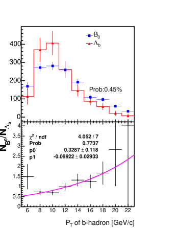
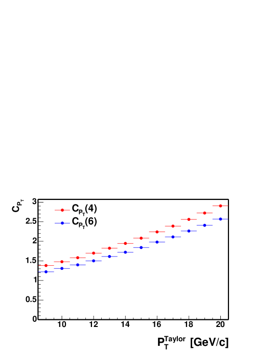
Figure 7.2: Comparison of $B^{0}$ and $\Lambda_{b}$ $P_{T}$ spectra measured in the data. The positive slope (2 $\sigma$ away from zero) of the ratio of $B^{0}$ to $\Lambda_{b}$ histograms indicates that $P_{T}(B^{0})$ is harder than $P_{T}(\Lambda_{b})$.

Figure 7.3: $\frac{\sigma_{\Lambda_{b}}}{\sigma_{B^{0}}}$ correction factor, $C_{P_{T}}$, as a function of $P_{T}^{\mathrm{Taylor}}$. The two curves represent the correction factor for two $P_{T}$ thresholds of $B$ hadrons: 4 $\rm GeV/c$ and 6 $\rm GeV/c$, respectively. $P_{T}^{\mathrm{Taylor}}$ is the $P_{T}$ threshold of $B$ hadrons in Taylor’s analysis.

7.2 Physics Backgrounds

Physics backgrounds come from the decays of $B$ hadrons into similar final state as our semileptonic signal: a $D^{*+}$ ($D^{+}$, $\Lambda_{c}^{+}$), a $\mu^{-}$ and missing particles. Branching ratios and efficiencies of these physics decays are needed to normalize the background contribution to the observed number of hadronic signal events in the data;

$$\frac{N_{\mathrm{physics}}}{N_{\mathrm{had}}}=\frac{\sum\;{\cal B}_{i}\cdot\epsilon_{i}}{{\cal B}_{\mathrm{had}}\cdot\epsilon_{had}}.$$ (7.21)

For the backgrounds to the $\overline{B}^{0}\rightarrow D^{*+}\mu^{-}\overline{\nu}_{\mu}$ and $\overline{B}^{0}\rightarrow D^{+}\mu^{-}\overline{\nu}_{\mu}$ decays, we find the modes which give similar final states as our semileptonic signals in the decays listed in the Particle Data Group (PDG) summary  [8] and the default decay table inside EvtGen package [75]. Many decays of $B$ and $D$ mesons have been measured by other experiments, such as CLEO, BELLE and BABAR. These measurements serve as inputs to the EvtGen decay package. Since BELLE and BABAR also use the EvtGen package, they have included decay modes into EvtGen which have not yet been measured and estimate the branching ratios. For the backgrounds to the $\Lambda_{b}\rightarrow\Lambda_{c}^{+}\mu^{-}\overline{\nu}_{\mu}$ decay, none of the $B$ hadrons decays to $\Lambda_{c}\mu$ final states have been measured in the CDF-I and other experiments, or estimated inside EvtGen. We use the results from the preliminary measurements by Litvintsev, et al. [86] and the prediction of PYTHIA to obtain the background branching ratios.

After we have a list of decays which share similar final states as our signals, we use the generator level simulation to estimate the composition of the inclusive semileptonic signal from each physics background. Details of this procedure maybe be found in the study by Tesarek, et al.[87][88]. The decays which contribute $\geq$ 1$\%$ to the semileptonic signal after trigger-like and the four track invariant mass $M_{D^{*}(D,\Lambda_{c})\mu}$ cuts are selected for further consideration. We generate each selected decay separately and run through the full CDF detector simulation as described in Section 6.1. Then we run the same signal reconstruction program used for the data on the MC and divide the number of reconstructed events by the number of generated events to obtain the efficiency.

7.2.1 Physics backgrounds of $\overline{B}^{0}\rightarrow D^{*+}\mu^{-}\overline{\nu}_{\mu}$ and $\overline{B}^{0}\rightarrow D^{+}\mu^{-}\overline{\nu}_{\mu}$

Physics backgrounds of $\overline{B}^{0}\rightarrow D^{*+}\mu^{-}\overline{\nu}_{\mu}$ and $\overline{B}^{0}\rightarrow D^{+}\mu^{-}\overline{\nu}_{\mu}$ fall into two categories:

1. Semileptonic decays of $B^{0}$, $B^{+}$, $B_{s}$, which include either additional particles (eg: $\overline{B}^{0}\rightarrow D^{+}\pi^{0}\mu^{-}\overline{\nu}_{\mu}$) or a higher mass charm meson with subsequent decay into our charm signal (eg: $\overline{B}^{0}\rightarrow D^{*+}\mu^{-}\overline{\nu}_{\mu}$, $D^{*+}\rightarrow D^{+}\pi^{0}$)

2. Hadronic $B^{0}$ decays into two charm mesons, one charm meson decays as our charm final state, the other charm meson decays semileptonically (eg: $\overline{B}^{0}\rightarrow D^{+}D_{s}^{-}$, $D_{s}^{-}\rightarrow\phi\mu^{-}\overline{\nu}_{\mu}$)

Tables 7.4– 7.4 summarize the physics background in $\overline{B}^{0}\rightarrow D^{*+}\mu^{-}\overline{\nu}_{\mu}$ and $\overline{B}^{0}\rightarrow D^{+}\mu^{-}\overline{\nu}_{\mu}$ which contribute $\geq$ 1$\%$. The second column in the table lists the measured or estimated branching ratios. All the numbers in parentheses are estimated uncertainties (100$\%$ for $B$ and 5$\%$ for charm) for the unmeasured branching fractions. The third column lists their efficiencies relative to the hadronic signals with statistical errors. The fourth column lists the normalization of each background relative to the exclusive semileptonic signal. The last column lists the number of events from each background after multiplying the relative branching ratio and efficiencies with the number of hadronic signal in the data, as expressed in Equation 7.21. The uncertainty in the last column only includes the statistical uncertainty of the hadronic yield. When normalizing backgrounds from $B^{+}$ and $B_{s}$ to $B^{0}$ signals, the following fragmentation fractions quoted in the 2004 PDG are used:

$$b\rightarrow B_{d} = (39.7\pm 1.3)\%,$$

$$b\rightarrow B_{u} = (39.7\pm 1.3)\%,$$

$$b\rightarrow B_{s} = (10.7\pm 1.1)\%.$$

Note that most of the backgrounds which contribute $\geq$ 1$\%$ share the same Feynman diagram as our semileptonic signal:

• resonant mode: a spectator quark and a $b$ to $c$ quark transition via a virtual $W$ boson exchange (eg: background of $\overline{B}^{0}\rightarrow D^{+}\mu^{-}\overline{\nu}_{\mu}$, $\overline{B}^{0}\rightarrow D^{*+}\mu^{-}\overline{\nu}_{\mu}$)

• non-resonant mode: with additional $u\overline{u}$ or $d\overline{d}$ quark pair created from the vacuum (eg: $\overline{B}^{0}\rightarrow D^{+}\pi^{0}\mu^{-}\overline{\nu}_{\mu}$)

Note that the non-resonant modes tend to have smaller branching ratios and smaller efficiencies than the resonant mode. The dominant background of $\overline{B}^{0}\rightarrow D^{*+}\mu^{-}\overline{\nu}_{\mu}$ is $B^{-}\rightarrow D_{1}^{0}\mu^{-}\overline{\nu}_{\mu}$ where $D_{1}^{0}\rightarrow D^{*+}\pi^{-}$. The total physics background in Table 7.4 is about 15$\%$ of $\overline{B}\rightarrow D^{*+}\mu^{-}X$ events in the data after all the cuts. The dominant background of $\overline{B}^{0}\rightarrow D^{+}\mu^{-}\overline{\nu}_{\mu}$ is $\overline{B}^{0}\rightarrow D^{*+}\mu^{-}\overline{\nu}_{\mu}$ where $D^{*+}\rightarrow D^{+}\pi^{0}$. The total physics background in Table 7.4 contributes about 40$\%$ of $\overline{B}\rightarrow D^{+}\mu^{-}X$ events in the data after all the cuts. As shown in Figure 7.4, a cut on the invariant mass of $D^{*+}$($D^{+}$)$\mu^{-}$ can reduce or eliminate the background from $B^{0}$, $B^{+}$ decaying semileptonically to more particles or a higher mass charm state.

Table 7.3: Physics backgrounds in $\overline{B}^{0}\rightarrow D^{*+}\mu^{-}\overline{\nu}_{\mu}$.

Mode	BR ($\%$)		$\epsilon$ ratio	Norm	$N_{event}$
$\overline{B}^{0}\rightarrow D^{*+}\pi^{-}$	0.276 $\pm$	0.021	1	–	$106$ $\pm$	$11$
$\overline{B}\rightarrow D^{*+}\mu^{-}X$	–		–	–	$1059$ $\pm$	$33$
$\overline{B}^{0}\rightarrow D^{*+}\mu^{-}\overline{\nu}_{\mu}$	5.44 $\pm$	0.23	0.447 $\pm$ 0.006	1.000	–
$B^{-}\rightarrow D_{1}^{0}\mu^{-}\overline{\nu}_{\mu}$	0.56 $\pm$	0.16	0.356 $\pm$ 0.008	0.055	51 $\pm$	5
$\hskip 36.0pt\hookrightarrow D^{*+}\pi^{-}$	66.67 $\pm$	(3.33)
$\overline{B}^{0}\rightarrow D_{1}^{+}\mu^{-}\overline{\nu}_{\mu}$	0.56 $\pm$	(0.56)	0.349 $\pm$ 0.008	0.027	25 $\pm$	3
$\hskip 36.0pt\hookrightarrow D^{*+}\pi^{0}$	33.33 $\pm$	(1.67)
$B^{-}\rightarrow D_{1}^{\prime 0}\mu^{-}\overline{\nu}_{\mu}$	0.37 $\pm$	(0.37)	0.351 $\pm$ 0.008	0.036	33 $\pm$	4
$\hskip 36.0pt\hookrightarrow D^{*+}\pi^{-}$	66.67 $\pm$	(3.33)
$\overline{B}^{0}\rightarrow D_{1}^{\prime+}\mu^{-}\overline{\nu}_{\mu}$	0.37 $\pm$	(0.37)	0.336 $\pm$ 0.008	0.017	16 $\pm$	2
$\hskip 36.0pt\hookrightarrow D^{*+}\pi^{0}$	33.33 $\pm$	(1.67)
$B^{-}\rightarrow D^{*+}\pi^{-}\mu^{-}\overline{\nu}_{\mu}$	0.20 $\pm$	(0.20)	0.242 $\pm$ 0.007	0.020	19 $\pm$	2
$\overline{B}^{0}\rightarrow D^{*+}\pi^{0}\mu^{-}\overline{\nu}_{\mu}$	0.10 $\pm$	(0.10)	0.239 $\pm$ 0.006	0.010	9 $\pm$	1
$\overline{B}^{0}\rightarrow D^{*+}\tau^{-}\overline{\nu}_{\tau}$	1.60 $\pm$	(1.60)	0.136 $\pm$ 0.005	0.016	15 $\pm$	2
$\hskip 54.0pt\hookrightarrow\mu^{-}\overline{\nu}_{\mu}$	17.36 $\pm$	0.06

Table 7.4: Physics backgrounds in $\overline{B}^{0}\rightarrow D^{+}\mu^{-}\overline{\nu}_{\mu}$.

Mode	BR ($\%$)		$\epsilon$ ratio	Norm	$N_{event}$
$\overline{B}^{0}\rightarrow D^{+}\pi^{-}$	0.276 $\pm$	0.025	1.000	–	$579$ $\pm$	$30$
$\overline{B}\rightarrow D^{+}\mu^{-}X$	–		–	–	$4720$ $\pm$	$100$
$\overline{B}^{0}\rightarrow D^{+}\mu^{-}\overline{\nu}_{\mu}$	2.14 $\pm$	0.20	0.455 $\pm$ 0.004	1.000	–
$\overline{B}^{0}\rightarrow D^{*+}\mu^{-}\overline{\nu}_{\mu}$	5.44 $\pm$	0.23	0.372 $\pm$ 0.005	0.671	1373 $\pm$	71
$\hskip 36.0pt\hookrightarrow D^{+}\pi^{0}/\gamma$	32.30 $\pm$	0.64
$\overline{B}^{0}\rightarrow D^{+}\pi^{0}\mu^{-}\overline{\nu}_{\mu}$	0.30 $\pm$	(0.30)	0.165 $\pm$ 0.004	0.051	104 $\pm$	5
$B^{-}\rightarrow D^{+}\pi^{-}\mu^{-}\overline{\nu}_{\mu}$	0.60 $\pm$	(0.60)	0.165 $\pm$ 0.004	0.102	208 $\pm$	11
$B^{-}\rightarrow D_{1}^{0}\mu^{-}\overline{\nu}_{\mu}$	0.56 $\pm$	0.16	0.278 $\pm$ 0.005	0.034	70 $\pm$	4
$\hskip 36.0pt\hookrightarrow D^{*+}\pi^{-}$	66.67 $\pm$	(3.33)
$\hskip 60.0pt\hookrightarrow D^{+}\pi^{0}/\gamma$	32.30 $\pm$	0.64
$B^{-}\rightarrow D_{1}^{0}\mu^{-}\overline{\nu}_{\mu}$	0.37 $\pm$	(0.37)	0.273 $\pm$ 0.005	0.022	46 $\pm$	3
$\hskip 36.0pt\hookrightarrow D^{*+}\pi^{-}$	66.67 $\pm$	(3.33)
$\hskip 60.0pt\hookrightarrow D^{+}\pi^{0}/\gamma$	32.30 $\pm$	0.64
$\overline{B}^{0}\rightarrow D^{+}\tau^{-}\overline{\nu}_{\tau}$	0.70 $\pm$	(0.70)	0.100 $\pm$ 0.004	0.013	26 $\pm$	1
$\hskip 54.0pt\hookrightarrow\mu^{-}\overline{\nu}_{\mu}$	17.36 $\pm$	0.06
$\overline{B}_{s}\rightarrow D^{+}K^{0}\mu^{-}\overline{\nu}_{\mu}$	0.30 $\pm$	(0.30)	0.137 $\pm$ 0.005	0.011	23 $\pm$	1

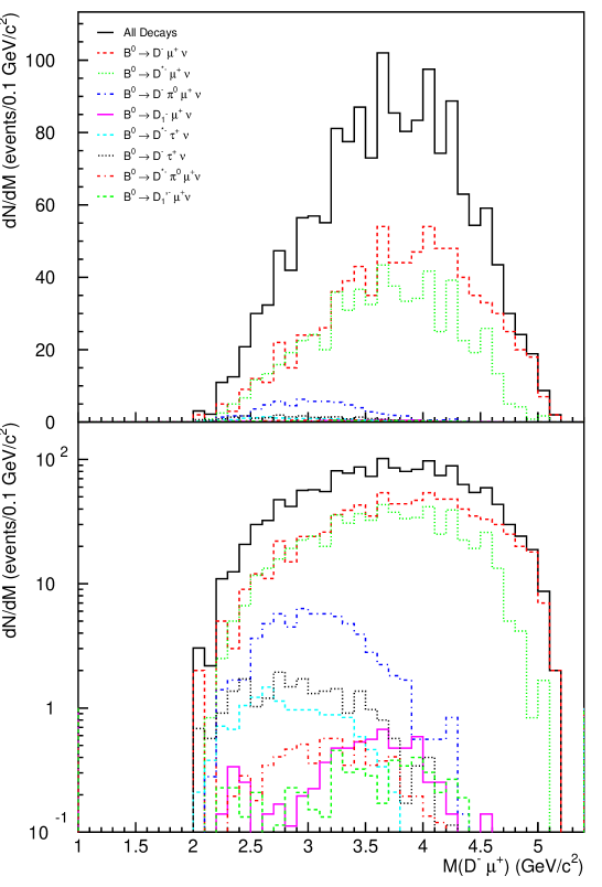
Figure 7.4: Invariant mass of $D^{+}\mu^{-}$ for the signal and physics backgrounds from semileptonic $B^{0}$ decays [87]. The top and bottom histograms are the same plot on a linear and log scale, respectively. Note that the backgrounds are concentrated in the low mass region. The signal to background ratio is larger at the higher mass region.

7.2.2 Physics backgrounds of $\Lambda_{b}\rightarrow\Lambda_{c}^{+}\mu^{-}\overline{\nu}_{\mu}$

Physics backgrounds of $\Lambda_{b}\rightarrow\Lambda_{c}^{+}\mu^{-}\overline{\nu}_{\mu}$ fall into two categories:

1. Other semileptonic decays of $\Lambda_{b}$, which either include additional particles (eg: $\Lambda_{b}\rightarrow\Lambda_{c}^{+}\pi^{+}\pi^{-}\mu^{-}\overline{\nu}_{\mu}$) or include a higher mass charm baryon with subsequent decay into our charm signal (eg: $\Lambda_{b}\rightarrow\Lambda_{c}(2593)^{+}\mu^{-}\overline{\nu}_{\mu}$, $\Lambda_{c}(2593)^{+}\rightarrow\Lambda_{c}^{+}\gamma$)

2. Baryonic semileptonic decays of $B_{u,d,s}$, which decay into $\Lambda_{c}^{+}$ or higher mass charm baryon, a proton or a neutron and leptons (eg: $B^{-}\rightarrow\Lambda_{c}^{+}\overline{p}\mu^{-}\overline{\nu}_{\mu}$)

Other $\Lambda_{b}$ Semileptonic Decays

We have learned from Section 7.2.1 that these physics backgrounds should have the same or similar Feynman diagrams as $\Lambda_{b}\rightarrow\Lambda_{c}^{+}\mu^{-}\overline{\nu}_{\mu}$. The observation of $\Lambda_{c}(2593)^{+}$ with spin $\frac{1}{2}$ and $\Lambda_{c}(2625)^{+}$ with spin $\frac{3}{2}$ [89] [90] indicates the existence of decays $\Lambda_{b}\rightarrow\Lambda_{c}(2593)^{+}\mu^{-}\overline{\nu}_{\mu}$ and $\Lambda_{b}\rightarrow\Lambda_{c}(2625)^{+}\mu^{-}\overline{\nu}_{\mu}$. Leibovich and Stewart [91] predict a range of the relative decay widths of $\Lambda_{b}$ to these two excited $\Lambda_{c}$ decays to the inclusive semileptonic decay, $\Lambda_{b}\rightarrow\Lambda_{c}^{+}\mu\;\mathrm{anything}$:

$$0.083<\frac{\Gamma(\Lambda_{b}\rightarrow\Lambda_{c}(2593)^{+}\mu^{-}\overline{\nu}_{\mu})}{\Gamma(\Lambda_{b}\rightarrow\Lambda_{c}^{+}\mu\;\mathrm{anything})}<0.248,$$

$$0.079<\frac{\Gamma(\Lambda_{b}\rightarrow\Lambda_{c}(2625)^{+}\mu^{-}\overline{\nu}_{\mu})}{\Gamma(\Lambda_{b}\rightarrow\Lambda_{c}^{+}\mu\;\mathrm{anything})}<0.166.$$

However, the wide range gives a systematic uncertainty as large as 100$\%$. In addition, the following decays have similar Feynman diagrams as $\Lambda_{b}\rightarrow\Lambda_{c}(2593)^{+}\mu^{-}\overline{\nu}_{\mu}$ and $\Lambda_{b}\rightarrow\Lambda_{c}(2625)^{+}\mu^{-}\overline{\nu}_{\mu}$:

$\Lambda_{b}\rightarrow\Lambda_{c}^{+}f^{0}\mu^{-}\overline{\nu}_{\mu}$,	$\Lambda_{b}\rightarrow\Sigma_{c}^{0}\pi^{+}\mu^{-}\overline{\nu}_{\mu}$,
$\Lambda_{b}\rightarrow\Lambda_{c}^{+}\pi^{0}\pi^{0}\mu^{-}\overline{\nu}_{\mu}$,	$\Lambda_{b}\rightarrow\Sigma_{c}^{+}\pi^{0}\mu^{-}\overline{\nu}_{\mu}$,
$\Lambda_{b}\rightarrow\Lambda_{c}^{+}\pi^{+}\pi^{-}\mu^{-}\overline{\nu}_{\mu}$,	$\Lambda_{b}\rightarrow\Sigma_{c}^{++}\pi^{-}\mu^{-}\overline{\nu}_{\mu}$.

Corresponding decays in the $\tau$ channel can also produce contamination in our semileptonic signal, as seen in Section 7.2.1.

In order to reduce the systematic uncertainties due to the branching ratios of these backgrounds, Litvintsev reconstructed the following decays [86]:

$\Lambda_{b}\rightarrow\Lambda_{c}(2593)^{+}\mu^{-}\overline{\nu}_{\mu}$,	$\Lambda_{b}\rightarrow\Lambda_{c}(2625)^{+}\mu^{-}\overline{\nu}_{\mu}$,
$\Lambda_{b}\rightarrow\Sigma_{c}^{0}\pi^{+}\mu^{-}\overline{\nu}_{\mu}$,	$\Lambda_{b}\rightarrow\Sigma_{c}^{++}\pi^{-}\mu^{-}\overline{\nu}_{\mu}$,

using the data processed with the Production executable, version 5.3.1, and compressed into the secondary datasets xbhd0d and xbhd0e. The cuts applied in Litvintsev’s analysis are similar to the ones for this analysis. After taking into account the efficiency difference between the reconstructed backgrounds and the $\Lambda_{b}\rightarrow\Lambda_{c}^{+}\mu^{-}\overline{\nu}_{\mu}$, we extract the relative branching ratios of these backgrounds to the $\Lambda_{b}\rightarrow\Lambda_{c}^{+}\mu^{-}\overline{\nu}_{\mu}$:

$$\frac{{\cal B}(\Lambda_{b}\rightarrow\Lambda_{c}(2593)^{+}\mu^{-}\overline{\nu}_{\mu})}{{\cal B}(\Lambda_{b}\rightarrow\Lambda_{c}^{+}\mu^{-}\overline{\nu}_{\mu})} = (4.7\pm 1.6)\times 10^{-2},$$ (7.22)

$$\frac{{\cal B}(\Lambda_{b}\rightarrow\Lambda_{c}(2625)^{+}\mu^{-}\overline{\nu}_{\mu})}{{\cal B}(\Lambda_{b}\rightarrow\Lambda_{c}^{+}\mu^{-}\overline{\nu}_{\mu})} = (7.9\pm 1.5)\times 10^{-2},$$ (7.23)

$$\frac{{\cal B}(\Lambda_{b}\rightarrow\Sigma_{c}^{0}\pi^{+}\mu^{-}\overline{\nu}_{\mu})}{{\cal B}(\Lambda_{b}\rightarrow\Lambda_{c}^{+}\mu^{-}\overline{\nu}_{\mu})} = (4.2\pm 1.6)\times 10^{-2},$$ (7.24)

$$\frac{{\cal B}(\Lambda_{b}\rightarrow\Sigma_{c}^{++}\pi^{-}\mu^{-}\overline{\nu}_{\mu})}{{\cal B}(\Lambda_{b}\rightarrow\Lambda_{c}^{+}\mu^{-}\overline{\nu}_{\mu})} = (4.2\pm 1.6)\times 10^{-2}.$$ (7.25)

Assuming the isospin symmetry, we can infer

$$\frac{{\cal B}(\Lambda_{b}\rightarrow\Sigma_{c}^{+}\pi^{0}\mu^{-}\overline{\nu}_{\mu})}{{\cal B}(\Lambda_{b}\rightarrow\Lambda_{c}^{+}\mu^{-}\overline{\nu}_{\mu})}=(4.2\pm 1.6)\times 10^{-2}.$$

However, we need the input of ${\cal B}(\Lambda_{b}\rightarrow\Lambda_{c}^{+}\mu^{-}\overline{\nu}_{\mu})$ to obtain the absolute branching fractions of the decays listed above. Assuming heavy quark symmetry, we expect the semileptonic decay width for all $B$ hadrons are the same, i.e. $\Gamma^{\mathrm{semi}}_{\Lambda_{b}}=\Gamma^{\mathrm{semi}}_{B^{0}}=\Gamma^{\mathrm{semi}}_{B^{+}}=\Gamma^{\mathrm{semi}}_{B_{s}}$. Then, the semileptonic branching ratios of the $B$ hadrons, $\Gamma^{\mathrm{semi}}/\Gamma^{\mathrm{total}}$, only vary due to the lifetime difference which result in a difference in $\Gamma^{\mathrm{total}}$. Since the $\Lambda_{b}$ decays to a spin-$\frac{1}{2}$ $\Lambda_{c}$, we expect contributions from both S and P wave amplitudes. Taking a weighted average of ${\cal B}(\overline{B}^{0}\rightarrow D^{+}\mu\nu+D^{*+}\mu\nu)$ and ${\cal B}(B^{-}\rightarrow D^{0}\mu\nu+\rightarrow D^{*0}\mu\nu)$, where the branching ratios of the $D^{+}$ and $D^{0}$ ($D^{*+}$ and $D^{*0}$) final states correspond to the S (P) wave amplitudes, we obtain 7.83 $\pm$ 0.26 $\%$. We further scale the number by the ratio of lifetimes, $\frac{\tau_{\Lambda_{b}}}{<\tau_{B}>}=0.80$, and estimate ${\cal B}(\Lambda_{b}\rightarrow\Lambda_{c}^{+}\mu^{-}\overline{\nu}_{\mu})$= ($6.26$ $\pm$ $0.21$)$\%$. For the ${\cal B}(\Lambda_{b}\rightarrow\Lambda_{c}^{+}\tau^{-}\overline{\nu}_{\tau})$, we multiply ${\cal B}(\Lambda_{b}\rightarrow\Lambda_{c}^{+}\mu^{-}\overline{\nu}_{\mu})$ by the ratio of phase space $\frac{Ph.Sp.(\Lambda_{b}\rightarrow\Lambda_{c}^{+}\tau^{-}\overline{\nu}_{\tau})}{Ph.Sp.(\Lambda_{b}\rightarrow\Lambda_{c}^{+}\mu^{-}\overline{\nu}_{\mu})}=0.277$.

Adding the branching fractions of $\Lambda_{b}$ to $\Lambda_{c}$, $\Lambda_{c}(2596)$, $\Lambda_{c}(2625)$, $\Sigma_{c}^{0,+,++}$ semileptonic decays in the $\mu$ and $\tau$ channels after correcting for the ${\cal B}(\tau\rightarrow\mu\overline{\nu}_{\mu}\nu_{\tau})=17.36\pm 0.06\%$, we get 8.2$\%$. The branching ratio of the inclusive $\Lambda_{b}$ semileptonic decays in the 2004 PDG is:

$${\cal B}(\Lambda_{b}\rightarrow\Lambda_{c}^{+}\mu\;\mathrm{anything})=9.2\pm 2.1\%.$$

We fill the difference, 1.0$\%$, with the following decays:

$\Lambda_{b}\rightarrow\Lambda_{c}^{+}f^{0}\mu^{-}\overline{\nu}_{\mu}$,

$\Lambda_{b}\rightarrow\Lambda_{c}^{+}\pi^{0}\pi^{0}\mu^{-}\overline{\nu}_{\mu}$,

$\Lambda_{b}\rightarrow\Lambda_{c}^{+}\pi^{+}\pi^{-}\mu^{-}\overline{\nu}_{\mu}$,

where the branching fraction of $\Lambda_{b}\rightarrow\Lambda_{c}^{+}\pi^{+}\pi^{-}\mu^{-}\overline{\nu}_{\mu}$ is estimated to be twice of $\Lambda_{b}\rightarrow\Lambda_{c}^{+}\pi^{0}\pi^{0}\mu^{-}\overline{\nu}_{\mu}$ based on the isospin invariance. A more detailed description about the estimate of these $\Lambda_{b}$ semileptonic decays can be found in Tesarek [88]. Table 7.5 summarizes the physics background from the $\Lambda_{b}$ semileptonic decays discussed above and their relative efficiencies to the hadronic signal. The dominant backgrounds are $\Lambda_{b}\rightarrow\Lambda_{c}(2593)^{+}\mu^{-}\overline{\nu}_{\mu}$ and $\Lambda_{b}\rightarrow\Lambda_{c}(2625)^{+}\mu^{-}\overline{\nu}_{\mu}$. Total physics background in Table 7.5 is about 9.2$\%$ of the $\overline{B}\rightarrow\Lambda_{c}^{+}\mu^{-}X$ events in the data.

Table 7.5: Physics backgrounds in $\Lambda_{b}\rightarrow\Lambda_{c}^{+}\mu^{-}\overline{\nu}_{\mu}$ from other $\Lambda_{b}$ semileptonic decays.

Mode	BR ($\%$)		$\epsilon$ ratio	Norm	$N_{event}$
$\Lambda_{b}\rightarrow\Lambda_{c}^{+}\pi^{-}$	$0.41$ $\pm$	0.21	1	–	$179$ $\pm$	$19$
$\overline{B}\rightarrow\Lambda_{c}^{+}\mu^{-}X$	–		–	–	$1237$ $\pm$	$97$
$\Lambda_{b}\rightarrow\Lambda_{c}^{+}\mu^{-}\overline{\nu}_{\mu}$	$6.26$ $\pm$	$0.21$	0.300 $\pm$ 0.004	1	–
$\Lambda_{b}\rightarrow\Lambda_{c}(2593)^{+}\mu^{-}\overline{\nu}_{\mu}$	$0.30$ $\pm$	$0.13$	0.196 $\pm$ 0.003	0.031	26 $\pm$	3
$\hskip 36.0pt\hookrightarrow\Sigma_{c}^{++}\pi^{-}$	24  $\pm$	7
$\hskip 60.0pt\hookrightarrow\Lambda_{c}^{+}\pi^{+}$	100
$\hskip 36.0pt\hookrightarrow\Sigma_{c}^{0}\pi^{+}$	24  $\pm$	7
$\hskip 60.0pt\hookrightarrow\Lambda_{c}^{+}\pi^{-}$	100
$\hskip 36.0pt\hookrightarrow\Sigma_{c}^{+}\pi^{0}$	24  $\pm$	(1.2)
$\hskip 60.0pt\hookrightarrow\Lambda_{c}^{+}\pi^{0}$	100
$\hskip 36.0pt\hookrightarrow\Lambda_{c}^{+}\pi^{+}\pi^{-}$	18  $\pm$	10
$\hskip 36.0pt\hookrightarrow\Lambda_{c}^{+}\pi^{0}\pi^{0}$	9  $\pm$	(0.45)
$\hskip 36.0pt\hookrightarrow\Lambda_{c}^{+}\gamma$	1  $\pm$	(0.05)
$\Lambda_{b}\rightarrow\Lambda_{c}(2625)^{+}\mu^{-}\overline{\nu}_{\mu}$	$0.49$ $\pm$	$0.17$	0.191 $\pm$ 0.003	0.050	42 $\pm$	4
$\hskip 36.0pt\hookrightarrow\Lambda_{c}^{+}\pi^{+}\pi^{-}$	66  $\pm$	(3.3)
$\hskip 36.0pt\hookrightarrow\Lambda_{c}^{+}\pi^{0}\pi^{0}$	33  $\pm$	(1.7)
$\hskip 36.0pt\hookrightarrow\Lambda_{c}^{+}\gamma$	1  $\pm$	(0.05)
$\Lambda_{b}\rightarrow\Lambda_{c}^{+}f^{0}\mu^{-}\overline{\nu}_{\mu}$	$0.25$ $\pm$	($0.25$)	0.023 $\pm$ 0.002	0.003	2.6 $\pm$	0.3
$\Lambda_{b}\rightarrow\Lambda_{c}^{+}\pi^{+}\pi^{-}\mu^{-}\overline{\nu}_{\mu}$	$0.50$ $\pm$	($0.50$)	0.032 $\pm$ 0.002	0.009	7 $\pm$	1
$\Lambda_{b}\rightarrow\Lambda_{c}^{+}\pi^{0}\pi^{0}\mu^{-}\overline{\nu}_{\mu}$	$0.25$ $\pm$	($0.25$)	0.033 $\pm$ 0.002	0.004	3.6 $\pm$	0.4
$\Lambda_{b}\rightarrow\Sigma_{c}^{0}\pi^{+}\mu^{-}\overline{\nu}_{\mu}$	$0.26$ $\pm$	$0.13$	0.081 $\pm$ 0.004	0.011	10 $\pm$	1
$\hskip 36.0pt\hookrightarrow\Lambda_{c}^{+}\pi^{-}$	100
$\Lambda_{b}\rightarrow\Sigma_{c}^{+}\pi^{0}\mu^{-}\overline{\nu}_{\mu}$	$0.26$ $\pm$	$0.13$	0.072 $\pm$ 0.004	0.010	8 $\pm$	1
$\hskip 36.0pt\hookrightarrow\Lambda_{c}^{+}\pi^{0}$	100
$\Lambda_{b}\rightarrow\Sigma_{c}^{++}\pi^{-}\mu^{-}\overline{\nu}_{\mu}$	$0.26$ $\pm$	$0.13$	0.077 $\pm$ 0.004	0.011	9 $\pm$	1
$\hskip 36.0pt\hookrightarrow\Lambda_{c}^{+}\pi^{+}$	100
$\Lambda_{b}\rightarrow\Lambda_{c}^{+}\tau^{-}\overline{\nu}_{\tau}$	$1.74$ $\pm$	($1.74$)	0.040 $\pm$ 0.003	0.007	5 $\pm$	1
$\hskip 48.0pt\hookrightarrow\mu^{-}\overline{\nu}_{\mu}$	17.36 $\pm$	0.06

$B$ Meson Baryonic Semileptonic Decays

While there are branching ratio measurements of the $B$ baryonic hadronic decay, eg: $\overline{B}^{0}\rightarrow\Lambda_{c}^{+}\overline{p}\pi^{+}\pi^{-}$, there is only an upper limit for the semileptonic decay of $B_{u}/B_{d}$ mixture:

$${\cal B}(B^{0}/B^{+}\rightarrow\Lambda_{c}^{-}pe\nu_{e})<0.15\%.$$

In order to obtain a list of $B$ meson baryonic semileptonic decays that could contribute to our signal, we make use of the predictions from the PYTHIA. We generate $B^{0}$, $B^{+}$, and $B_{s}$ mesons using PYTHIA. We force the mesons to decay semileptonically and let PYTHIA handle the fragmentation. We count the number of events for each specific $B$ meson to $\Lambda_{c}^{+}$ decay, and find the maximum contributions are from the decays $B^{-}\rightarrow\Lambda_{c}^{+}\overline{p}\mu^{-}\overline{\nu}_{\mu}$ and $\overline{B}^{0}\rightarrow\Lambda_{c}^{+}\overline{n}\mu^{-}\overline{\nu}_{\mu}$. We assume the upper limit for the muon-neutron or muon-proton final state should be the same as those decays with a proton and electron in the final state (see above). The value of this upper limit is then used for each branching fraction of $B^{-}\rightarrow\Lambda_{c}^{+}\overline{p}\mu^{-}\overline{\nu}_{\mu}$ and $\overline{B}^{0}\rightarrow\Lambda_{c}^{+}\overline{n}\mu^{-}\overline{\nu}_{\mu}$.

We obtain the efficiencies for these two decays from the MC. Since we find the $P_{T}$ spectra of $B$ mesons and $\Lambda_{b}$ are quite different, it is least ambiguous to calculate the quantity:

$$\frac{N_{B^{-}\rightarrow\Lambda_{c}^{+}\overline{p}\mu^{-}\overline{\nu}_{\mu}}}{N_{\Lambda_{b}\rightarrow\Lambda_{c}^{+}\pi^{-}}}=\frac{\sigma_{\Lambda_{b}}(P_{T}>4.0)}{\sigma_{B^{0}}(P_{T}>4.0)}\cdot\frac{{\cal B}(B^{-}\rightarrow\Lambda_{c}^{+}\overline{p}\mu^{-}\overline{\nu}_{\mu})\cdot\epsilon_{B^{-}\rightarrow\Lambda_{c}^{+}\overline{p}\mu^{-}\overline{\nu}_{\mu}}}{{\cal B}(\Lambda_{b}\rightarrow\Lambda_{c}^{+}\pi^{-})\cdot\epsilon_{\Lambda_{b}\rightarrow\Lambda_{c}^{+}\pi^{-}}},$$ (7.26)

where the production cross section ratio is the $\rho(4)$ in Equation 7.18. We use a low $P_{T}$ threshold ($P_{T}$ $>$ 4 $\rm GeV/c$) because we wish to accurately assess the acceptance of the $B$ hadron after applying the reconstruction requirements. Specifically we are concerned about the case where the neutrino is emitted in the direction opposite to the direction that $B$ hadron is traveling. This case increases the $P_{T}$ of the remaining daughters and may make their total $P_{T}$ greater than the $P_{T}$ of the $B$ hadron. Therefore, the denominator of the efficiency is the number of events with $B$ mesons or $\Lambda_{b}$ $P_{T}$ $>$ 4 $\rm GeV/c$ and rapidity $<$ 2.0. The numerator is the number of events which pass all the trigger and analysis cuts. Table 7.6 summarizes the $B$ meson to $\Lambda_{c}^{+}$$\mu^{-}$ backgrounds. The contribution of $B^{0}$ and $B^{+}$ in the $\overline{B}\rightarrow\Lambda_{c}^{+}\mu^{-}X$ events is about 0.4$\%$ each.

Table 7.6: Physics backgrounds in $\Lambda_{b}\rightarrow\Lambda_{c}^{+}\mu^{-}\overline{\nu}_{\mu}$ from $B$ mesons.

Mode	BR ($\%$)		Relative $\epsilon$	Norm	$N_{event}$
$\Lambda_{b}\rightarrow\Lambda_{c}^{+}\pi^{-}$	$0.41$ $\pm$	0.21	1	–	$179$  $\pm$	$19$
$\overline{B}\rightarrow\Lambda_{c}^{+}\mu^{-}X$	–		–	–	$1237$  $\pm$	$97$
$\Lambda_{b}\rightarrow\Lambda_{c}^{+}\mu^{-}\overline{\nu}_{\mu}$	$6.26$ $\pm$	$0.21$	0.265 $\pm$ 0.004	1	–
$B^{-}\rightarrow\Lambda_{c}^{+}\overline{p}\mu^{-}\overline{\nu}_{\mu}$	0.15 $\pm$	(0.15)	0.045 $\pm$ 0.002	0.006	4.7 $\pm$	0.5
$\overline{B}^{0}\rightarrow\Lambda_{c}^{+}\overline{n}\mu^{-}\overline{\nu}_{\mu}$	0.15 $\pm$	(0.15)	0.044 $\pm$ 0.002	0.006	4.6 $\pm$	0.5

7.3 Fake Muons

Another source of background originates from a charm hadron together with a hadron track ($\pi$, $K$, proton) misidentified as a muon. A hadron is misidentified as a muon when it has higher energy and punches through the hadron calorimeter, or when it decays into a muon before being stopped in the hadron calorimeter via decays like $\pi^{+}\rightarrow\mu^{+}\nu_{\mu}$, $K^{+}\rightarrow\mu^{+}\nu_{\mu}$ or $K^{+}\rightarrow\pi^{0}\mu^{+}\nu_{\mu}$. Physics processes that generate these hadrons are direct production, inelastic collisions with the detector material, fragmentation or the decays of charm and $B$ hadrons. Fragmentation is the process by which a $b$ or $c$ quark combines with additional quarks and gluons to form a $q\overline{q}$ or $qqq$ bound state. Fake muons from the first three categories tend to have a softer $P_{T}$ spectrum than the real muons from $B$ decays. A tighter $P_{T}$ cut on the muon candidate largely removes these backgrounds. Fake muons from the charm hadrons which are produced at the primary vertex are also suppressed. For the reason that we require the muon candidate should be matched to an SVT track with a $d_{0}$ greater than 120 $\mu$m, while fake muons from the promptly produced charm tend to have smaller impact parameter. Also for the reason that we require the charm hadron and the muon candidate to form a vertex displaced from the beam line and make a strict requirement on the pseudo $c\tau$.

$$\mathrm{pseudo}\;c\tau\ =\frac{M_{B}}{P_{T}(\mathrm{charm}+\mu)}\cdot L_{xy}.$$ (7.27)

Here $P_{T}(\mathrm{charm}+\mu)$ is the total transverse momentum of charm hadron and the muon.

Therefore, our principle source of fake muons comes from two types of $B$ hadron decays:

• $\overline{B}\rightarrow D^{*+}\ (D^{+},\Lambda_{c}^{+})X_{\mathrm{had}}\;\mathrm{anything}$: hadronic decays of any $B$ hadrons, where $X_{\mathrm{had}}$ is $\pi$, $K$ or proton which fakes the muon.

• $\overline{B}\rightarrow D^{*+}\ (D^{+},\Lambda_{c}^{+})X_{\mathrm{had}}\;l\;\overline{\nu}_{l}\;\mathrm{anything}$: semileptonic $B$ decay into a charm, a hadron track $X_{\mathrm{had}}$, and any leptons ($e$, $\mu$, $\tau$). The muon is not reconstructed but $X_{\mathrm{had}}$ fakes the muon.

In this section, we estimate the fake muon contamination for our three signals: $\overline{B}^{0}\rightarrow D^{*+}\mu^{-}\overline{\nu}_{\mu}$, $\overline{B}^{0}\rightarrow D^{+}\mu^{-}\overline{\nu}_{\mu}$ and $\Lambda_{b}\rightarrow\Lambda_{c}^{+}\mu^{-}\overline{\nu}_{\mu}$. Note the charge conjugates of the modes listed are also included.

7.3.1 Background Estimate

We use two methods to estimate the amount of contamination from fake muons in our semileptonic signal. Each method uses a different way to obtain the number of (hadron track, charm hadron) candidates in our data. Both methods apply the previous CDF measurements of the probabilities for a real pion, kaon and proton to be misidentified as a muon. These measurements are performed by Ashmanskas and Harr [92] using a pion and kaon sample from the $D^{*+}\rightarrow D^{0}\pi^{+}$decays, where $D^{0}\rightarrow K^{-}\pi^{+}$, and by Litvintsev [93] using a proton sample from the $\Lambda\rightarrow p^{+}\pi^{-}$ decays. The fake probability ${\cal P}_{\pi}$ (${\cal P}_{K}$, ${\cal P}_{p}$) is defined as the number of pions (kaons or protons) that pass the following muon identification cuts divided by the total number of pions (kaons or protons) inside the fiducial volume of CDF Central Muon Detector (CMU) and matched to an SVT track.

• The track is fiducial to the CMU and matched to an SVT track

• The track is associated with hits in the CMU

• The matching $\chi^{2}$ between the track and the hits in the CMU is less than 9.

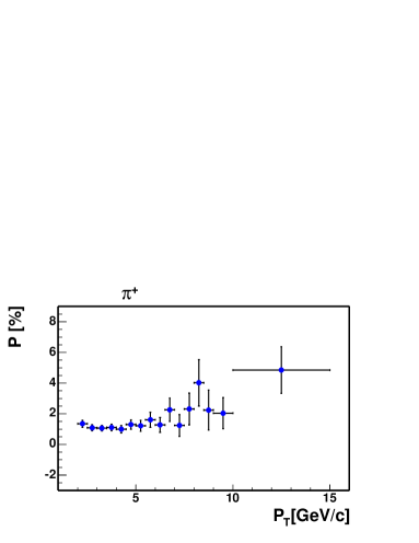
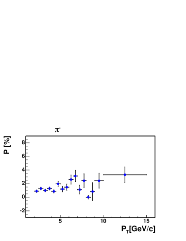
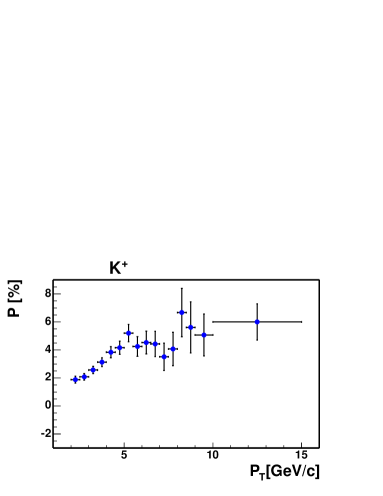
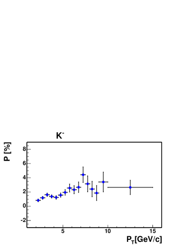
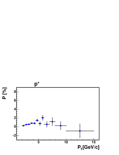
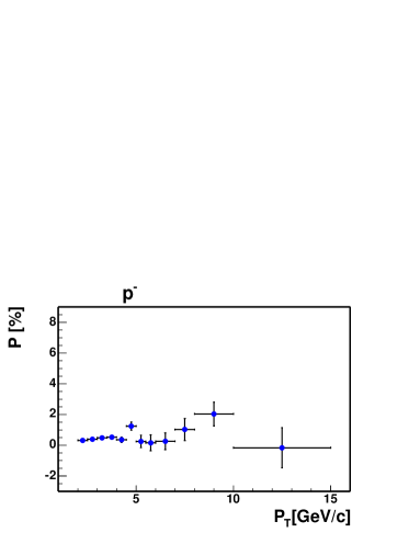
Figure 7.5: The probability for a pion, kaon or proton being misidentified as a muon in bins of transverse momentum ($P_{T}$) from the measurements by Ashmanskas, Harr  [92] and Litvintsev[93]. From the top left to the bottom right are $\pi^{+}$, $\pi^{-}$, $K^{+}$, $K^{-}$, $p$ and $\overline{p}$ fake probabilities.

Figure 7.5 shows the ${\cal P}_{\pi}$, ${\cal P}_{K}$ measured in sixteen and ${\cal P}_{p}$ measured in twelve transverse momentum bins for positive and negative charged tracks, separately.

Method I

The first method uses data to obtain the number of (hadron track,charm hadron) candidates, then Monte Carlo to determine the ratio of pions, kaons and protons in the hadron tracks. We run the same signal reconstruction program on the secondary datasets hbot0h and hbot1i. We do not use the skimmed tertiary datasets (see Yu [64] ) as the samples are biased by requiring at least one track in the event matched to a muon stub in the muon detector. We look for a charged track which fails the muon identification cuts (TRK^fail). TRK^fail and a charm hadron should form a displaced vertex and pass the same analysis cuts we apply to the signal. Each event is weighted with the fake probability (${\cal P}_{\mathrm{avg}}$) according to the momentum and the charge of TRK^fail. We then fit the weighted charm hadron mass distribution, i.e. $M_{K\pi\pi}-M_{K\pi}$, $M_{K\pi\pi}$ and $M_{pK\pi}$, using the same functions as described in Section 5.1, to obtain the signal contamination from the fake muons. Since an event-weighted likelihood fit will not give a proper error for the yield, a binned $\chi^{2}$ fit is performed. ${\cal P}_{\mathrm{avg}}$ is a weighted average of pion, kaon and proton fake probability (${\cal P}_{\pi}$, ${\cal P}_{K}$, ${\cal P}_{p}$). The weight $R_{i}$ is determined by the fraction of pions, kaons and protons in the $\overline{B}\rightarrow D^{*+}\ (D^{+},\Lambda_{c}^{+})X_{\mathrm{had}}\;l\;\overline{\nu}_{l}\;\mathrm{anything}$ and $\overline{B}\rightarrow D^{*+}\ (D^{+},\Lambda_{c}^{+})X_{\mathrm{had}}\;\mathrm{anything}$ MC after analysis cuts:

$${\cal P}_{\mathrm{avg}}=R_{\pi}{\cal P}_{\pi}+R_{K}{\cal P}_{K}+R_{p}{\cal P}_{p},$$ (7.28)

where

$$R_{i}=\frac{N_{i}}{N_{\pi}+N_{K}+N_{p}},$$

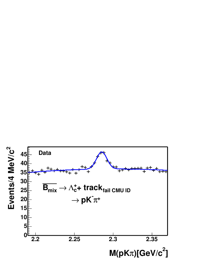
Figure 7.6: Fit of $\overline{B}\rightarrow\Lambda_{c}^{+}\mu_{\mathrm{fake}}$ yield after weighting the charged track which fails the muon ID cut with an average muon fake probability. There 40 $\pm$ 6 events in the peak. Fit $\chi^{2}/\mathrm{NDF}$ = 55.6/39, probability = 4.1$\%$. A sideband subtraction yields 44 $\pm$ 25 events in the signal peak.

and $i$ is $\pi$, $K$ or proton. The Monte Carlo is generated as described in Section 6.1. Decays of $B^{0}$, $B^{+}$, $B_{s}$ and $\Lambda_{b}$ are generated separately and decay tables include all the possible decays. Each kind of $B$ hadron gives different $R_{i}$ and is weighted with the product of the production fractions, total branching ratios and the number of generated events. Table 7.8 summarizes the pion to kaon ratio and the number of fake muon candidates before and after weighting the events in our three different signals. See Figure 7.6 for the weighted mass distribution of the $\Lambda_{b}$ mode.

The uncertainties of the number of fake muon candidates come from three sources: 1. the uncertainty from the binned $\chi^{2}$ fit, 2. the uncertainties on the pion, kaon and proton fractions due to the finite Monte Carlo sample size, the uncertainties of the branching ratios and production fractions, and 3. the uncertainty on the measured fake probability. For the last source, we vary the fake rate in each momentum bin $\pm$ 1 sigma, independently. We then add the systematic shifts in quadrature to get the accumulative uncertainty. The number of fake muons using this method is about 3–5$\%$ of the inclusive semileptonic signals in the data.

Method II

The second method relies on the MC and the external input of the branching ratios from the Particle Data Group (PDG) [8]. MC is run through the same reconstruction program for the data. Then we apply the same cuts as signal reconstruction and obtain the trigger and reconstruction efficiencies of $\overline{B}\rightarrow D^{*+}\ (D^{+},\Lambda_{c}^{+})X_{\mathrm{had}}\;\mathrm{anything}$ and $\overline{B}\rightarrow D^{*+}\ (D^{+},\Lambda_{c}^{+})X_{\mathrm{had}}\;l\;\overline{\nu}_{l}\;\mathrm{anything}$ decays. We weight the MC events which pass the analysis cuts with the fake probability according to the momentum, the charge and the particle type of the track, $X_{\mathrm{had}}$. The particle identification of the track, $X_{\mathrm{had}}$, is obtained by matching the hits on the reconstructed track with those on the input simulated track. Together with the efficiency of hadronic mode, branching ratios of our hadronic signals, $\overline{B}\rightarrow D^{*+}\ (D^{+},\Lambda_{c}^{+})X_{\mathrm{had}}\;\mathrm{anything}$ and $\overline{B}\rightarrow D^{*+}\ (D^{+},\Lambda_{c}^{+})X_{\mathrm{had}}\;l\;\overline{\nu}_{l}\;\mathrm{anything}$ from the PDG, we normalize the background to the observed number of hadronic signals in the data,

$$\frac{N_{\mathrm{fake}\;\mu}}{N_{\mathrm{had}}}=\frac{{\cal B}(\overline{B}\rightarrow D^{*+}\ (D^{+},\Lambda_{c}^{+})X)\cdot\epsilon_{\mathrm{fake}\;\mu}}{f_{d,\mathrm{baryon}}\cdot{\cal B}_{\mathrm{had}}\epsilon_{\mathrm{had}}}.$$ (7.29)

Equations 7.30– 7.31 use $D^{+}$ as an example to show how we derive the $\overline{B}\rightarrow D^{*+}\ (D^{+},\Lambda_{c}^{+})X_{\mathrm{had}}\;\mathrm{anything}$ and $\overline{B}\rightarrow D^{*+}\ (D^{+},\Lambda_{c}^{+})X_{\mathrm{had}}\;l\;\overline{\nu}_{l}\;\mathrm{anything}$ branching ratios from the existing information in the PDG.

$${\cal B}(\overline{B}\rightarrow D^{+}X_{\mathrm{had}}\;l\nu_{l}\;\mathrm{anything}) = \frac{7}{3}\cdot{\cal B}(\overline{B}\rightarrow D^{+}\pi^{+}\mu\;\mathrm{anything})$$ (7.30)

$$+ \frac{7}{3}\cdot{\cal B}(\overline{B}\rightarrow D^{+}\pi^{-}\mu\;\mathrm{anything}),$$

$${\cal B}(\overline{B}\rightarrow D^{+}X_{\mathrm{had}}\;\mathrm{anything}) = {\cal B}(\overline{B}\rightarrow D^{+}\mathrm{anything})$$ (7.31)

$$- \frac{7}{3}\cdot{\cal B}(\overline{B}\rightarrow D^{+}\mu\;\mathrm{anything}),$$

where the factor, $\frac{7}{3}$, comes from the fact that the branching ratios of muon and electron channels are equal and the branching ratio of the tau channel is scaled down by the ratio of the phase space, $\sim\frac{1}{3}$. Therefore, we have to scale up the branching ratio of the muon channel by $1+1+\frac{1}{3}=\frac{7}{3}$ to get the total branching ratio of all the lepton channels.

Table 7.8 summarizes the parameters used to calculate the number of fake muon events, where the decay $\overline{B}\rightarrow D^{*+}\ (D^{+},\Lambda_{c}^{+})X_{\mathrm{had}}\;\mathrm{anything}$ is denoted as mode “1” and $\overline{B}\rightarrow D^{*+}\ (D^{+},\Lambda_{c}^{+})X_{\mathrm{had}}\;l\;\overline{\nu}_{l}\;\mathrm{anything}$ is denoted as mode “2” in the table. The uncertainties on the number of fake muons originate from: the uncertainty on the hadronic yield, the relative efficiency, the uncertainty on the fake rate and the relative branching ratios. The dominant uncertainty is from the relative branching ratios. The number of fake muon backgrounds from method I is consistent with the result using method II. We use the results of method I in the calculation of our final result of the relative branching ratios. In general, the fraction of fake muons is about 5$\%$ of the total semileptonic yield in the data.

Table 7.7: Parameters for the number of fake muons: Method I.

	$\overline{B}^{0}\rightarrow D^{*+}\mu^{-}\overline{\nu}_{\mu}$	$\overline{B}^{0}\rightarrow D^{+}\mu^{-}\overline{\nu}_{\mu}$	$\Lambda_{b}\rightarrow\Lambda_{c}^{+}\mu^{-}\overline{\nu}_{\mu}$
N before weighting	2953 $\pm$ 57	15343 $\pm$ 303	3560 $\pm$ 198
$R_{\pi}$	0.937 $\pm$ 0.009	0.909 $\pm$ 0.005	0.71 $\pm$ 0.16
$R_{K}$	0.063 $\pm$ 0.009	0.091 $\pm$ 0.005	0.05 $\pm$ 0.08
$R_{p}$	–	–	0.24 $\pm$ 0.16
$N_{\mathrm{fake}\;\mu}$	44 $\pm$ 3	230 $\pm$ 19	40 $\pm$ 9

Table 7.8: Parameters for the number of fake muons: Method II.

	$\overline{B}^{0}\rightarrow D^{*+}\mu^{-}\overline{\nu}_{\mu}$	$\overline{B}^{0}\rightarrow D^{+}\mu^{-}\overline{\nu}_{\mu}$	$\Lambda_{b}\rightarrow\Lambda_{c}^{+}\mu^{-}\overline{\nu}_{\mu}$
${\cal B}_{\mathrm{had}}$ $\%$	0.276 $\pm$ 0.021	0.276 $\pm$ 0.025	$0.41\pm 0.19$
${\cal B}_{1}$ $\%$	10.9 $\pm$ 2.1	17.7 $\pm$ 2.4	4.8 $\pm$ 3.0
$\frac{\epsilon_{1}}{\epsilon_{\mathrm{had}}}$	0.0038 $\pm$ 0.0004	0.0022 $\pm$ 0.0002	0.0029 $\pm$ 0.0003
${\cal B}_{2}$ $\%$	1.3 $\pm$ 0.3	1.8 $\pm$ 0.6	$<$ 1.23
$\frac{\epsilon_{2}}{\epsilon_{\mathrm{had}}}$	0.0005 $\pm$ 0.0002	0.0010 $\pm$ 0.0002	0.0002 $\pm$ 0.0001
$N_{\mathrm{had}}$	$106\ \pm 11$	$579\ \pm 30$	$179\ \pm 19$
$N_{\mathrm{fake}\;\mu}$	45 $\pm$ 11	220 $\pm$ 41	28 $\pm$ 34

Like-sign Combination

Note that we do not use the like sign combination (i.e. the charm hadron and the muon have the same sign of charges) to estimate the fake muon background for two reasons: First, two different $B$ hadrons from the $b\overline{b}$ in the event can produce a real muon and a real charm of the same charge sign when the $B$ hadrons in the event have opposite flavors and one $B$ hadron decays semileptonically. Second, the two track trigger, used for this analysis, requires a pair of tracks with opposite charges. The trigger requirement greatly reduces the number of like-sign (wrong-sign) candidates and introduces large statistical errors for the number of fake muons.

Fake muons from $b\overline{b}$ and $c\overline{c}$

One type of fake muons is not included in the previous subsections. These fake muons stem from $b\overline{b}$, $c\overline{c}$ to two $B$ or charm hadrons then decay into a charm signal, a hadron track misidentified as a muon and other missing particles. A study at the generator level for the $\overline{B}^{0}\rightarrow D^{+}\mu^{-}\overline{\nu}_{\mu}$ mode is done using the $b\overline{b}$ and $c\overline{c}$ PYTHIA [71] Monte Carlo datasets as described in Section 7.4.2. We apply analysis-like cuts on the Monte Carlo. We weight the events that pass the cuts with the muon fake probability according to the “muon” candidate momentum, charge and the true particle identification: a kaon, a pion or a proton. Then we compare the number of weighted events with the number of charm hadron and real muon combinations, i.e, a $b\overline{b}$ and $c\overline{c}$ background as described in Section 7.4. We find that fake muons from $b\overline{b}$ and $c\overline{c}$ is about 10$\%$ of the $b\overline{b}$ and $c\overline{c}$ background with real muons. See Table 7.9. From Section 7.4, we show that the $b\overline{b}$ and $c\overline{c}$ background with real muons is at the 1$\%$ level. Therefore, we conclude that $b\overline{b}$ and $c\overline{c}$ background with fake muons is about or less than 0.1$\%$ and can be ignored.

Table 7.9: Fake muons from $b\overline{b}$ and $c\overline{c}$.

	$b\overline{b}$	$c\overline{c}$
Ngen	43454949	89718181
Real muon Npass	15	35
Fake muon Npass	1.8	0.4

7.4 $b\overline{b}$ and $c\overline{c}$ Backgrounds

When the azimuthal angle ($\Delta\phi$) between $b\overline{b}$ or $c\overline{c}$ quark pair is small, daughters of two heavy flavor hadrons from the fragmentation of $b\overline{b}$ or $c\overline{c}$ appear to come from the same decay vertex, see Figure 7.7 . Here $\Delta\phi$ is defined as the opening angle in the plane perpendicular to the proton and antiproton beam axis. If one hadron decays semileptonically, and the other hadron decays into a charm final state, such as $D^{*+}\rightarrow D^{0}\pi^{+}$, $D^{+}\rightarrow K^{-}\pi^{+}\pi^{+}$, and $\Lambda_{c}^{+}\rightarrow pK^{-}\pi^{+}$, the muon from the semileptonic decay, together with the charm, may fake our semileptonic signal. Production mechanisms and an estimate of the amount of $b\overline{b}$ and $c\overline{c}$ backgrounds are discussed below.

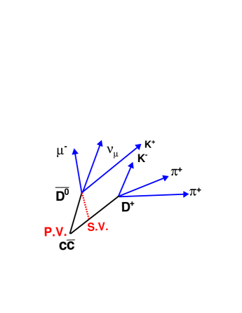
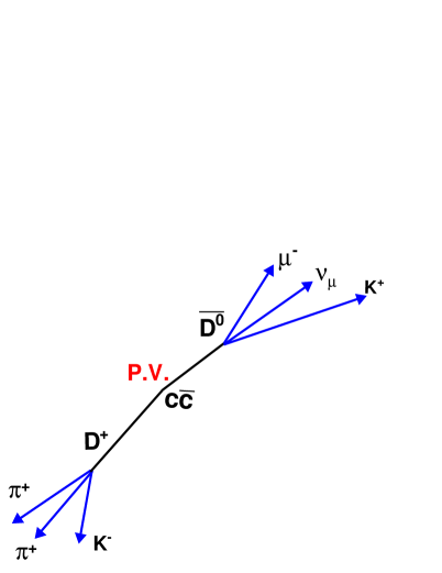
Figure 7.7: Charm hadrons from $c\overline{c}$ with small (left) and big (right) $\Delta\phi$. In the left figure, the muon from the semileptonic decay of $\overline{D}^{0}$ and the $D^{+}$ forms a secondary vertex and fake our $\overline{B}^{0}\rightarrow D^{+}\mu^{-}\overline{\nu}_{\mu}$ signal. In the right figure, $\Delta\phi$ between two charm hadrons is too big and the daughters can not form a secondary vertex.

7.4.1 $b\overline{b}$ and $c\overline{c}$ Production Mechanism

In $p\overline{p}$ collisions, the b or c quarks may be single or pair produced by the electroweak and the strong (QCD) processes. The b or c quark production cross-section for the electroweak process $\sigma\cdot{\cal B}(p\overline{p}\rightarrow W\rightarrow bc)$ is around 0.01 $\mu b$ and is derived from the CDF measurement of the inclusive W cross-section by Halkiadakis, et al. [94]. The $b\overline{b}$ and $c\overline{c}$ production cross-sections for the QCD process are around 50 and 200$\mu b$ respectively from the PYTHIA [71] Monte Carlo, when the total transverse momenta of the hard scattering, i.e. the part of the interaction with the largest momentum scale, is greater than 5 $\rm GeV/c$ and at least one b or c quark has $P_{T}$ $>$ 4.0 $\rm GeV/c$, pseudo-rapidity $\eta$ $<$ 1.5. The $b\overline{b}$ and $c\overline{c}$ production rates from the electroweak process are about five thousand times smaller than the QCD processes. Therefore, only pair production by the QCD processes are discussed here.

Figure 7.8 shows the leading and next-to-leading order Feynman diagrams for $b\overline{b}$($c\overline{c}$) production by the QCD processes from Lannon[95]. The QCD process that contributes the production at leading order is flavor creation; which includes quark anti-quark annihilation ($q\overline{q}\rightarrow$ $b\overline{b}$ or $c\overline{c}$) and gluon fusion ($gg\rightarrow$ $b\overline{b}$ or $c\overline{c}$). The distribution of the azimuthal angle ($\Delta\phi$) between two produced b(c) quarks peaks at 180 degrees. The reason is that the $q$ and $\overline{q}$ (or $g$ and $g$) come from the proton and the anti-proton separately. The initial total momenta of the gluon $q\overline{q}$ pair is zero. The $b\overline{b}$ ($c\overline{c}$) pair are produced back-to-back to balance the momentum in the final state.

The next-to-leading order (NLO) processes, flavor excitation and gluon splitting, contribute at the same level as the flavor creation [95]. Flavor excitation refers to the following process: The gluons within one of the beam particles in the initial state split into a $b\overline{b}$ ($c\overline{c}$) pair. One of b(c) quarks is scattered out of the initial state into the final state by a gluon or a light quark from the other beam particle. The other b(c) quark is not involved in the hard scattering process. The $\Delta\phi$ of $b\overline{b}$ ($c\overline{c}$) from flavor excitation is more evenly distributed than flavor creation.

Gluon splitting refers to the process when no b(c) quarks are involved in the hard scattering. One gluon in the final state splits into $b\overline{b}$ ($c\overline{c}$) pair. If the gluon is soft, $\Delta\phi$ will be a flat distribution. If the gluon is hard, the daughters of the gluon, $b\overline{b}$ ($c\overline{c}$) tend to move co-linearly and have small $\Delta\phi$. Figure 7.9 shows the azimuthal angle distribution between two b quarks from the study of Field [96] using PYTHIA CTEQ4L prediction.

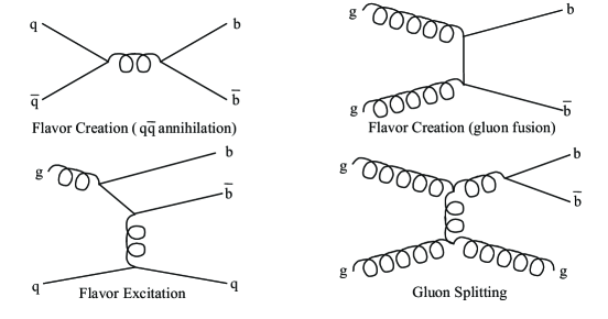
Figure 7.8: Representative lowest order Feynman diagrams (without loops or radiative corrections) of quark annihilation, gluon fusion, flavor excitation and gluon splitting. Details of these processes may be found in Lannon[95].

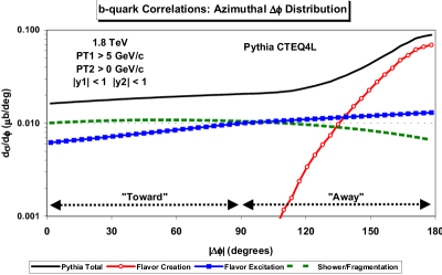
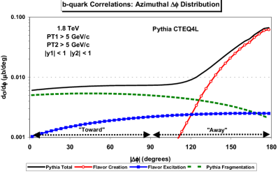
Figure 7.9: $\Delta\phi$ between $b$ and $\overline{b}$ from the study of Field  [96] using PYTHIA CTEQ4L. Both b quarks have $|y|$ $<$ 1. In the top plot, one b quark has $P_{T}$ $>$ 5 $\rm GeV/c$ and the other b quark does not have any $P_{T}$ cut. In the bottom plot, both b quarks have $P_{T}$ $>$ 5 $\rm GeV/c$.

7.4.2 Background Estimate

The amount of $b\overline{b}$ and $c\overline{c}$ background is normalized to the number of events observed in the hadronic modes in the the data,

$$\frac{N_{b\overline{b},c\overline{c}}}{N_{\mathrm{had}}}=\frac{\sigma_{b\overline{b},c\overline{c}}\cdot\sum_{i}\sum_{j}f^{i}{\cal B}_{j}\epsilon_{j}}{\sigma_{B^{0},\Lambda_{b}}\cdot{\cal B}_{\mathrm{had}}\epsilon_{\mathrm{had}}}.$$ (7.32)

Here, $i$ represents the species of b(c) hadrons and $j$ represents the decay modes which could contribute to $b\overline{b}$ and $c\overline{c}$ backgrounds. $f^{i}$ stands for the production fraction ratio for species $i$. ${\cal B}_{j}$ and $\epsilon_{j}$ are the branching ratio and the efficiency of $j^{th}$ decay mode. The following subsections detail the methods to estimate $\sigma_{b\overline{b},c\overline{c}}\cdot\sum_{i}\sum_{j}f^{i}{\cal B}_{j}\epsilon_{j}$ and $\sigma_{B^{0},\Lambda_{b}}\cdot{\cal B}_{\mathrm{had}}\epsilon_{\mathrm{had}}$ in Equation 7.32. We do not use detector and trigger simulations to obtain the efficiencies for the following reasons: First, detector and trigger simulations are time and CPU intensive. Second, we will find the contribution of this background is quite small compared with the other backgrounds. Third, we care about the efficiency ratio of the background to the signal, not the absolute efficiency. Our studies show that generator level Monte Carlo gives a good approximation. For instance, the relative efficiency $\frac{\epsilon(\Lambda_{b}\rightarrow\Lambda_{c}^{+}\pi^{-})}{\epsilon(\Lambda_{b}\rightarrow\Lambda_{c}^{+}\mu^{-}\overline{\nu}_{\mu})}$ is 3.31 $\pm$ 0.05 from the full detector simulation and 3.23 $\pm$ 0.01 from the generator level simulation. The difference is only about 2.5$\%$. Similar results are obtained from the relative efficiencies of our other signals.

Background: $\sigma_{b\overline{b},c\overline{c}}\cdot\sum_{i}\sum_{j}f^{i}{\cal B}_{j}\epsilon_{j}$

Our estimate of $\sigma_{b\overline{b},c\overline{c}}\cdot\sum_{i}\sum_{j}f^{i}{\cal B}_{j}\epsilon_{j}$ relies heavily on the Monte Carlo. We use PYTHIA version 6.2 [71] and to generate $b\overline{b}$ and $c\overline{c}$ events, we include the QCD processes mentioned in Section 7.4.1: flavor creation, flavor excitation and gluon splitting (MSEL=1). We further require the $P_{T}$ of the hard scattering be greater than 5 $\rm GeV/c$. Events with $b$ quarks $P_{T}$ greater than 4.0 $\rm GeV/c$ and pseudo-rapidity less than 1.5 are collected into the nbot90 sample. Events with $c$ quarks which satisfy the same kinematic cuts are collected into the nbota0 sample. Note that nbot90 and nbota0 have small overlap when both $b$ and $c$ quarks are produced and are above the $P_{T}$ and pseudo-rapidity thresholds. Details of nbot90 and nbota0 datasets could be found in [97]. PYTHIA $b\overline{b}$ and $c\overline{c}$ cross-sections are used for $\sigma_{b\overline{b},c\overline{c}}$.

The product of the efficiency, branching ratio and production fraction from all the modes, $\sum_{i}\sum_{j}f^{i}{\cal B}_{j}\epsilon_{j}$, is obtained using the following steps: First, we identify the $b\overline{b}$ ($c\overline{c}$) production mechanism to which we are most sensitive. In this pass, we only study the background that forms a $D^{+}\mu^{-}$ signature since $D^{+}$ has longer lifetime than $D^{*+}$, $\Lambda_{c}^{+}$ and $\overline{B}^{0}\rightarrow D^{+}\mu^{-}\overline{\nu}_{\mu}$ suffers larger $c\overline{c}$ background contamination compared to the other two modes. We need to achieve higher accuracy for the estimate of $\sum_{i}\sum_{j}f^{i}{\cal B}_{j}\epsilon_{j}$. Consequently, for the $b\overline{b}$ background, we re-decay nbot90 sample ten times, i.e. we re-use the same kinematic distribution of the parent hadrons from nbot90 ten times but decay the hadrons with independent random numbers and force the decay $D^{+}\rightarrow K^{-}\pi^{+}\pi^{+}$. For the $c\overline{c}$ background, we force the decay of $D^{+}\rightarrow K^{-}\pi^{+}\pi^{+}$ and require that all the negative charged charm hadron decay semileptonically.

Then, a generator level two track trigger filter (SvtFilter) is applied. We further identify any combination of $D^{+}$ and a muon which passes the generator-level, analysis-like cuts found in Table 7.11. In order to avoid double counting (count $c\overline{c}$ as $b\overline{b}$ background in nbot90 and $b\overline{b}$ as $c\overline{c}$ background in nbota0) due to the overlap of nbot90 and nbota0 samples, the ancestors of the muon and charm hadrons are retrieved by tracing the true information from the generator. If both muon and charm hadron come from the same $B$ hadron, the combination is rejected. If the muon and charm hadron come from different $B$ hadrons, the combination is categorized into $b\overline{b}$ background, otherwise, the combination is categorized as a $c\overline{c}$ background. We find that for both $b\overline{b}$ and $c\overline{c}$, more than 90$\%$ of the events that pass the cuts are from gluon splitting. Therefore, we are most sensitive to the “gluon splitting” mechanism. Table 7.10 summarizes the background contributions from different production processes.

Table 7.10: Summary of $b\overline{b}$ and $c\overline{c}$ production mechanisms and our relative sensitivity for reconstructing the event in our semileptonic sample.

	$b\overline{b}$ background	$c\overline{c}$ background
Ngen	219093011	21996889
Npass	75	62
Ngluon	70	57
Nexcitation	5	5
Ncreation	0	0
f${}_{gluon}(\%)$	93 $\pm$ 3	92 $\pm$ 3
f${}_{excitation}(\%)$	7 $\pm$ 3	8 $\pm$ 4
f${}_{creation}(\%)$	0	0

Second, we filter the gluon splitting events and re-decay the b(c) hadrons in nbot90 and nbota0 ten times with the procedure described above. For the $b\overline{b}$ background estimate, we let all the b hadrons and negative charged charm hadrons decay freely, but force the decays of the positive charged charm hadrons in two ways:

• $D^{*+}\rightarrow D^{0}\pi^{+}$, $D^{0}\rightarrow K^{-}\pi^{+}$ for the background of $\overline{B}^{0}\rightarrow D^{*+}\mu^{-}\overline{\nu}_{\mu}$

• $D^{+}\rightarrow K^{-}\pi^{+}\pi^{+}$ and $\Lambda_{c}^{+}\rightarrow pK^{-}\pi^{+}$ for the background of $\overline{B}^{0}\rightarrow D^{+}\mu^{-}\overline{\nu}_{\mu}$ and $\Lambda_{b}\rightarrow\Lambda_{c}^{+}\mu^{-}\overline{\nu}_{\mu}$

Then the SvtFilter and the cuts listed in Table 7.11 are applied. We divide the number of reconstructed events by the number of generated events and get $\sum_{i}\sum_{j}f^{i}{\cal B}_{j}\epsilon_{j}$. Table 7.13 lists the parameters for the $b\overline{b}$ background.

For the $c\overline{c}$ background estimate, we force the decays of both positive and negative charged charm hadrons. The positive charged charm hadrons are forced to decay into the modes listed above. The negative charged charm hadrons are forced to decay into semileptonic modes individually for $D^{-}$, $\overline{D}^{0}$, $D_{s}^{-}$ and $\Lambda_{c}^{-}$. As the semileptonic decay modes of these four charm hadrons are all different, we separate the events into four classes denoted by the parent charm particles. After applying SvtFilter and the cuts listed in Table 7.11, we obtain $\sum_{j}f^{i}{\cal B}_{j}\epsilon_{j}$ for each class. Then we multiply the semileptonic branching ratios for each kind of charm hadron with its $\sum_{j}f^{i}{\cal B}_{j}\epsilon_{j}$ and sum them up to get the total amount of $\sum_{j}f^{i}{\cal B}_{j}\epsilon_{j}$ for the $c\overline{c}$ background,

$$\sum_{i}\sum_{j}f^{i}{\cal B}_{j}\epsilon_{j}(total) = \sum_{i}\sum_{j}f^{i}{\cal B}_{j}\epsilon_{j}(D^{-}){\cal B}(D^{-}\rightarrow\mu X)$$ (7.33)

$$+\sum_{i}\sum_{j}f^{i}{\cal B}_{j}\epsilon_{j}(\overline{D}^{0}){\cal B}(\overline{D}^{0}\rightarrow\mu X)$$

$$+\sum_{i}\sum_{j}f^{i}{\cal B}_{j}\epsilon_{j}(D_{s}^{-}){\cal B}(D_{s}^{-}\rightarrow\mu X)$$

$$+\sum_{i}\sum_{j}f^{i}{\cal B}_{j}\epsilon_{j}(\Lambda_{c}^{-}){\cal B}(\Lambda_{c}^{-}\rightarrow\mu X).$$

Table 7.13 lists the parameters for the $c\overline{c}$ background.

In both $b\overline{b}$ and $c\overline{c}$ background estimates, since we force the positive charged charm hadron to decay into the same final state as our charm signals, we have to multiply the final result by two to include the contribution from both charge states. Table 7.15 lists $N_{b\overline{b}}$ and $N_{c\overline{c}}$ in our three different signals after multiplying the ratio in Equation 7.32 with the observed number of events in the hadronic signals.

Table 7.11: Generator-level analysis-like cuts for $b\overline{b}$ and $c\overline{c}$ background study.

Parameter	Cut Value
$P_{T}$ of all tracks	$>$ 0.5 $\rm GeV/c$
$P_{T}$ of $\mu$ ($\pi_{B}$)	$>$ 2.0 $\rm GeV/c$
$\eta$ of all tracks	$<$ 1.2
$\eta$ of $\mu$ ($\pi_{B}$)	$<$ 0.6
$P_{T}$ of four tracks	$>$ 6.0 $\rm GeV/c$
$P_{T}$ of charm hadron	$>$ 5.0 $\rm GeV/c$
$c\tau$ of four tracks	$>$ 200 $\mu$m (B), $>$ 250 $\mu$m ($\Lambda_{b}$)
$c\tau$ of charm hadron	$>$ -70 $\mu$m ($D^{*}$, $\Lambda_{c}$), $>$ -30 $\mu$m ($D^{+}$)
3.0 $<$ $M_{D^{(}*)\mu}$ $<$ 5.5 ${\rm GeV}/{\rm c}^{2}$
3.7 $<$ $M_{\Lambda_{c}\mu}$ $<$ 5.7 ${\rm GeV}/{\rm c}^{2}$
$\mu$ ($\pi_{B}$) match to a SVT track
charm hadron and $\mu$ ($\pi_{B}$) have opposite charge signs
2 out of 4 tracks of $B$ candidate pass two track trigger cuts

Table 7.12: Parameters used for $b\overline{b}$ background estimate.

PYTHIA $\sigma_{b\overline{b}}$ ($\mu$b)	49.6
	$b\overline{b}\ \rightarrow D^{*}\mu$	$b\overline{b}\ \rightarrow D\mu$	$b\overline{b}\ \rightarrow\Lambda_{c}\mu$
$N_{\mathrm{gen}}$	221606748	221619610	221619610
$N_{\mathrm{pass}}$	43	80	9
$\sum_{i}\sum_{j}f^{i}{\cal B}_{j}\epsilon_{j}$ (10-7)	1.9 $\pm$ 0.3	3.6 $\pm$ 0.4	0.41 $\pm$0.14
2 $\cdot$ $\sigma_{b\overline{b}}$ $\cdot$ $\sum_{i}\sum_{j}f^{i}{\cal B}_{j}\epsilon_{j}$ (10-5 $\mu$ b)	1.9 $\pm$ 0.3	3.6 $\pm$ 0.4	0.41 $\pm$ 0.14

Table 7.13: Parameters used for $c\overline{c}$ background estimate.

PYTHIA $\sigma_{c\overline{c}}$ ($\mu$b)	198.4
	$c\overline{c}\ \rightarrow D^{*}\mu$	$c\overline{c}\ \rightarrow D\mu$	$c\overline{c}\ \rightarrow\Lambda_{c}\mu$
$N_{\mathrm{gen}}$	720741510	698988700	698988700
$N_{\mathrm{pass}}$	214	396	7
$D^{-}$ : ${\cal B}(D^{-}\rightarrow\mu X)$ = 14.22 ($\%$)	117	205	4
$\overline{D}^{0}$ : ${\cal B}(\overline{D}^{0}\rightarrow\mu X)$ = 6.15 ($\%$)	76	157	2
$D_{s}^{-}$ : ${\cal B}(D_{s}^{-}\rightarrow\mu X)$ = 13.32 ($\%$)	19	34	1
$\Lambda_{c}^{-}$ : ${\cal B}(\Lambda_{c}^{-}\rightarrow\mu X)$ = 4.5 ($\%$)	2	0	0
$\sum_{i}\sum_{j}f^{i}{\cal B}_{j}\epsilon_{j}$ (10-8)	3.3 $\pm$ 0.6	6.2 $\pm$ 1.0	0.12 $\pm$ 0.05
2 $\cdot$ $\sigma_{c\overline{c}}$ $\cdot$ $\sum_{i}\sum_{j}f^{i}{\cal B}_{j}\epsilon_{j}$ (10-5 $\mu$ b)	1.3 $\pm$ 0.2	2.5 $\pm$ 0.4	0.047 $\pm$ 0.020

Hadronic signal: $\sigma_{B^{0},\Lambda_{b}}\cdot{\cal B}_{\mathrm{had}}\epsilon_{\mathrm{had}}$

In order to normalize the background to the observed number of events in the hadronic mode, the $B^{0}$ or $\Lambda_{b}$ production cross-section, the efficiency and the branching ratio of the hadronic signal, have to come from external input or must be calculated using MC (see Equation 7.32). We obtain $\sigma_{B^{0}}$ by multiplying the previous CDF $\sigma_{B^{+}}$ measurement by Keaffaber, et al. [98] with the production fraction ratios, $f_{d}/f_{u}$, from the 2004 PDG[8]. $B^{0}$ decay branching ratios are also obtained from the PDG. The product of $\sigma_{\Lambda_{b}}$ and ${\cal B}(\Lambda_{b}\rightarrow\Lambda_{c}^{+}\pi^{-})$ is obtained by multiplying the CDF measurement of $\frac{\sigma_{\Lambda_{b}}(P_{T}>6.0){\cal B}(\Lambda_{b}\rightarrow\Lambda_{c}^{+}\pi^{-})}{\sigma_{B^{0}}(P_{T}>6.0){\cal B}(\overline{B}^{0}\rightarrow D^{+}\pi^{-})}$ by Le, et al. [68] with the $\sigma_{B^{0}}$ we derive and the PDG ${\cal B}(\overline{B}^{0}\rightarrow D^{+}\pi^{-})$.

Since we reconstruct both b and anti-b hadrons in the data, we should multiply the measured cross-section by two. For the efficiencies, we use the MC to generate and decay $B$ hadrons into our signals as described in Section 6.1. The CDF $\sigma_{B^{+}}$ measurement is restricted to the $B^{+}$ with $P_{T}$ greater than 6 $\rm GeV/c$ and rapidity ($y$) less than 1.0. Therefore, the denominator of the efficiency is the number of events in which the $B$ hadrons have $P_{T}$ $>$ 6 $\rm GeV/c$ and $|y|$ $<$ 1.0. The numerator of the efficiency is the number of events which pass the cuts in Table 7.11 except the cut on four track invariant mass. Table 7.14 lists the parameters that are used to calculate $\sigma_{B^{0},\Lambda_{b}}\cdot{\cal B}_{\mathrm{had}}\epsilon_{\mathrm{had}}$.

Semileptonic signal

Table 7.14 also lists the efficiency and branching ratio of the semileptonic signal mode for a comparison with the background $N_{b\overline{b},c\overline{c}}$. In the case of the $\Lambda_{b}$, we lack the external input for the branching ratio of $\Lambda_{b}\rightarrow\Lambda_{c}^{+}\mu^{-}\overline{\nu}_{\mu}$. Therefore, instead of the exclusive mode, we list the branching ratio of the inclusive mode: $\overline{B}\rightarrow\Lambda_{c}^{+}\mu^{-}X$ from the 2004 PDG as an upper bound. We multiply the ratio $\rho(6)$ from Section 7.1 with the Keaffaber $\sigma_{B^{+}}$ result to get $\sigma_{\Lambda_{b}}$ for $P_{T}$ greater than 6.0 $\rm GeV/c$. The efficiency of $\Lambda_{b}\rightarrow\Lambda_{c}^{+}\mu^{-}\overline{\nu}_{\mu}$ is listed for a comparison with $\epsilon_{b\overline{b},c\overline{c}}$. Note that the amount of $b\overline{b}$ and $c\overline{c}$ background relative to the signal is around 1$\%$. The numbers from three different modes should not be compared directly without multiplying the branching ratios of the charm decays.

Table 7.14: Parameters used to calculate $\sigma_{B^{0},\Lambda_{b}}$, ${\cal B}_{had}\epsilon_{had}$ and ${\cal B}_{semi}\epsilon_{semi}$.

$\sigma_{B^{+}}$ ($\mu$b)	3.6 $\pm$ 0.6
	$\overline{B}\rightarrow D^{*+}X$	$\overline{B}\rightarrow D^{+}X$	$\Lambda_{b}\rightarrow\Lambda_{c}^{+}X$
$f_{x}/f_{u}$	1.00 $\pm$ 0.04	1.00 $\pm$ 0.04	0.25 $\pm$ 0.04
$\sigma_{B^{0},\Lambda_{b}}$ ($\mu$b)	3.6 $\pm$ 0.6	3.6 $\pm$ 0.6	2.2 $\pm$ 0.5
	$\overline{B}^{0}\rightarrow D^{*+}\pi^{-}$	$\overline{B}^{0}\rightarrow D^{+}\pi^{-}$	$\Lambda_{b}\rightarrow\Lambda_{c}^{+}\pi^{-}$
$\frac{\sigma_{\Lambda_{b}}(P_{T}>6.0){\cal B}(\Lambda_{b}\rightarrow\Lambda_{c}^{+}\pi^{-})}{\sigma_{B^{0}}(P_{T}>6.0){\cal B}(\overline{B}^{0}\rightarrow D^{+}\pi^{-})}$	–	–	0.82 $\pm$ 0.26
${\cal B}_{\mathrm{had}}$ ($\%$)	0.276 $\pm$ 0.021	0.276 $\pm$ 0.025	–
$\sigma(\Lambda_{b}){\cal B}(\Lambda_{b}\rightarrow\Lambda_{c}^{+}\pi^{-})$ ($\mu$b)	–	–	0.008 $\pm$ 0.003
$N_{\mathrm{gen}}$	4242100	4242100	39999996
$N_{\mathrm{pass}}$	70147	130433	843693
$\epsilon_{\mathrm{had}}$ (10-2)	1.654 $\pm$ 0.006	3.075 $\pm$ 0.008	2.109 $\pm$ 0.002
2$\sigma_{B^{0},\Lambda_{b}}{\cal B}_{had}\epsilon_{had}$ (10-5 $\mu$b)	33 $\pm$ 6	61 $\pm$ 12	34 $\pm$ 13
	$\overline{B}^{0}\rightarrow D^{*+}\mu^{-}\overline{\nu}_{\mu}$	$\overline{B}^{0}\rightarrow D^{+}\mu^{-}\overline{\nu}_{\mu}$	$\Lambda_{b}\rightarrow\Lambda_{c}^{+}\mu^{-}\overline{\nu}_{\mu}$
${\cal B}_{\mathrm{semi}}$ ($\%$)	5.44 $\pm$ 0.23	2.14 $\pm$ 0.20	9.2 $\pm$ 2.1 ($\%$)
$N_{\mathrm{gen}}$	4242100	4242100	39999996
$N_{\mathrm{pass}}$	32620	66854	264484
$\epsilon_{\mathrm{semi}}$ (10-2)	0.769 $\pm$ 0.004	1.576 $\pm$ 0.006	0.661 $\pm$ 0.001
2$\sigma_{B^{0},\Lambda_{b}}{\cal B}_{\mathrm{semi}}\epsilon_{\mathrm{semi}}$ (10-5 $\mu$b)	300 $\pm$ 50	240 $\pm$ 50	270 $\pm$ 90

Table 7.15: The amount of $b\overline{b}$ and $c\overline{c}$ background.

	$\overline{B}\rightarrow D^{*+}X$		$\overline{B}\rightarrow D^{+}X$		$\Lambda_{b}\rightarrow\Lambda_{c}^{+}X$
$N_{\mathrm{had}}$	$106$  $\pm$	$11$	$579$  $\pm$	$30$	$179$  $\pm$	$19$
$N_{\mathrm{semi}}$	$1059$  $\pm$	$33$	$4720$  $\pm$	$100$	$1237$  $\pm$	$97$
$N_{b\overline{b}}$	6  $\pm$	0.6	34  $\pm$	2	2.1 $\pm$	0.2
$N_{c\overline{c}}$	4  $\pm$	0.4	23  $\pm$	1	0.2 $\pm$	0.03

7.4.3 Comparison of Data and MC Cross Section

While there are precise measurements of the single charm hadron, $B^{+}$ and inclusive b hadron cross-sections, there are no accurate measurements of the total $b\overline{b}$ and $c\overline{c}$ cross-section ($\sigma_{b\overline{b}}$, $\sigma_{c\overline{c}}$) at the Tevatron, yet. To understand how well PYTHIA predicts $\sigma_{b\overline{b}}$ and $\sigma_{c\overline{c}}$, we cross-check indirectly by comparing the “differential cross-section” of $D^{0}$, $B^{+}$ and inclusive b hadrons in PYTHIA with CDF Run I and II measurements by Chen [99], Keaffaber[98], and Bishai [41] et al.. We count the number of $D^{0}$, $B^{+}$ or b hadrons from nbot90 and nbota0 in bins of $P_{T}(D^{0})$, $P_{T}(B^{+})$ and $P_{T}(J/\psi)$. The bin width and the $P_{T}$ ranges are the same as Chen, Keaffaber and Bishai analyses. We divide the number of hadrons in each $P_{T}$ bin by the total number of generated events. Then we multiply Pythia assumed $\sigma_{b\overline{b}}$ and $\sigma_{c\overline{c}}$ (see Tables 7.13– 7.13) to get the cross section of hadrons in each $P_{T}$ bin. We further divide the number by the bin width to obtain the “differential cross-section”. The agreements between Monte Carlo and data cross-sections are generally within 10$\%$ for charm hadrons and 40$\%$ for $B$ hadrons (see Figure 7.10).

Besides the total cross-section of $b\overline{b}$ and $c\overline{c}$, the ratio of gluon splitting relative to the other two processes, flavor creation and flavor excitation, also affects the amount of $b\overline{b}$ and $c\overline{c}$ backgrounds. Previous CDF Run I measurement of $b\overline{b}$ azimuthal production correlations by Lannon [100] concludes that Pythia gives reasonable prediction of the relative $b\overline{b}$ production rates from the three processes. However, due to the lack of measurements of the $c\overline{c}$ relative production rates, we do not yet have a comparison of the fraction of $c\overline{c}$ gluon splitting between Monte Carlo and data. Therefore, we assign 100$\%$ uncertainty when calculating the systematic errors for the estimate of $b\overline{b}$ and $c\overline{c}$ backgrounds. As the contribution of $b\overline{b}$ and $c\overline{c}$ background is at the 1$\%$ level, the systematic errors from 100$\%$ uncertainty is also about 1$\%$.

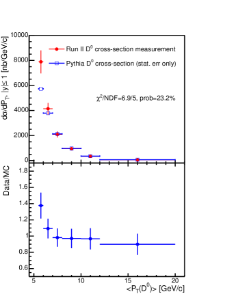
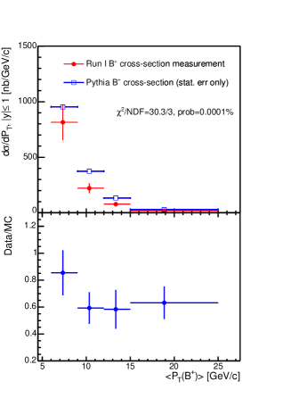
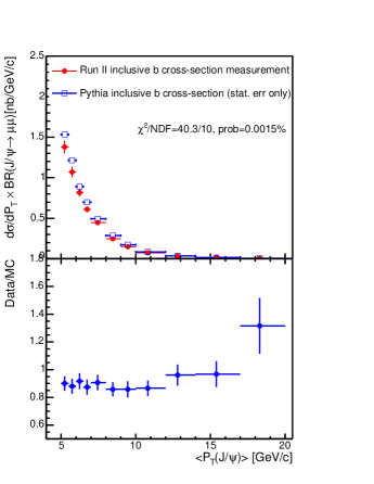
Figure 7.10: $D^{0}$ (top left), $B^{+}$ (top right), and inclusive $b$ (bottom) differential cross-sections. The upper plot in each figure shows the differential cross-section for data (closed circles) by Chen [99], Keaffaber [98], and Bishai [41] and MC (open squares). The lower plot in each figure shows the data to MC ratio.

7.4.4 Comparison of Data and MC Impact Parameter

We compare the distribution of the impact parameter of charm hadrons with respect to the beam spot in MC and data. Figure 7.11 shows a good agreement of the MC with the data. No excess of charm hadrons with small $d_{0}$ is found in the data. This indicates that the promptly produced charm from $c\overline{c}$ has negligible contribution to the background in the semileptonic $B$ decays, which is consistent with our estimate using PYTHIA.

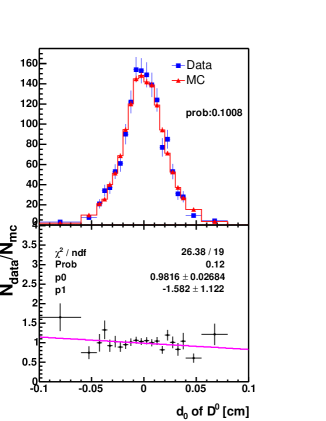
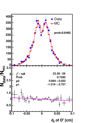
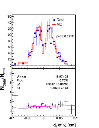
Figure 7.11: Impact parameters of the charm hadrons, from the top left to the bottom are $D^{0}$, $D^{+}$ and $\Lambda_{c}^{+}$: MC and data comparison. The good agreement of the MC with the data indicates that background from the promptly produced charm ($c\overline{c}$) is negligible.

7.5 Background Summary

The fraction of each type of background in our semileptonic signal is summarized below. The dominant signal contamination is from the physics background. The second largest background arises from muon fakes. The smallest background source is from $b\overline{b}$ and $c\overline{c}$.

Table 7.16: Summary of the backgrounds to the semileptonic modes.

	$N_{\mathrm{bg}}/N_{\mathrm{inc\;semi}}$ ($\%$)
Background Type	$D^{*}\mu$	$D\mu$	$\Lambda_{c}\mu$
Physics	15	40	9.8
Muon fakes	4.3	4.9	3.2
$b\overline{b}$ and $c\overline{c}$	0.9	1.2	0.2
Total	20.2	46.1	13.8

Chapter 8 Relative Branching Fraction Results and Systematics

Recall that the equation for the ratio of branching fractions is:

$$\frac{{\cal B}_{\mathrm{semi}}}{{\cal B}_{\mathrm{had}}}=(\frac{N_{\mathrm{inclusive\;semi}}-N_{\mathrm{physics}}-N_{\mathrm{fake\mu}}-N_{c\overline{c},\;b\overline{b}}}{N_{\mathrm{had}}})\times\frac{\epsilon_{\mathrm{had}}}{\epsilon_{\mathrm{semi}}},$$ (8.1)

where the yields, $N_{\mathrm{had}}$ and $N_{\mathrm{inclusive\;semi}}$, are obtained in Chapter 5. In Section 6.3, the efficiencies, $\epsilon_{\mathrm{had}}$ and $\epsilon_{\mathrm{semi}}$ are determined and in Chapter 7, the backgrounds to our semileptonic signals are estimated. We are now in a position to calculate the relative branching fractions. The relative branching fractions with the statistical uncertainties only are:

$$\frac{{\cal B}(\overline{B}^{0}\rightarrow D^{*+}\mu^{-}\overline{\nu}_{\mu})}{{\cal B}(\overline{B}^{0}\rightarrow D^{*+}\pi^{-})} = 17.7\ \pm 2.3,$$

$$\frac{{\cal B}(\overline{B}^{0}\rightarrow D^{+}\mu^{-}\overline{\nu}_{\mu})}{{\cal B}(\overline{B}^{0}\rightarrow D^{+}\pi^{-})} = 9.8\ \pm 1.0,$$

$$\frac{{\cal B}(\Lambda_{b}\rightarrow\Lambda_{c}^{+}\mu^{-}\overline{\nu}_{\mu})}{{\cal B}(\Lambda_{b}\rightarrow\Lambda_{c}^{+}\pi^{-})} = 20.0\ \pm 3.0.$$

In the remainder of this chapter, we first discuss and estimate the systematic uncertainties. Then, we show the result of the relative branching fractions for each mode. Finally, implications of our measurements are discussed and a conclusion is given at the end of the chapter.

8.1 Systematic Uncertainties

8.1.1 Sources of Systematics

Systematic uncertainties in our measurements may arise from the difference in the semileptonic and hadronic decays, from the lack of knowledge of certain backgrounds, and from the uncertainties on the external information. Most of the sources are common to all the decay modes. Systematic uncertainties which affect only one mode are discussed separately. To simplify the notation, we define our measurement of the relative branching fractions as $R$:

$$R\equiv\frac{{\cal B}_{\mathrm{semi}}}{{\cal B}_{\mathrm{had}}},$$

and $\sigma_{R}$ is the systematic uncertainty. We also denote the term, “branching ratio” in the text, as ${\cal BR}$, while the branching ratio of one specific mode is denoted as ${\cal B}(\mathrm{mode})$, eg: ${\cal B}(\overline{B}^{0}\rightarrow D^{+}\pi^{-})$.

Mass Fitting

• $\overline{B}\rightarrow D^{*+}\mu^{-}X$ and $\overline{B}\rightarrow\Lambda_{c}^{+}\mu^{-}X$: The mass functions are general and cover all the possible backgrounds. Because the functions do not involve any external ${\cal BR}$ or MC efficiencies, we do not assign systematic uncertainty for the mass fitting of these two modes.

• $\overline{B}\rightarrow D^{+}\mu^{-}X$: The uncertainties on the $D_{s}$ decay ${\cal BR}$ can modify the misreconstructed $D_{s}$ mass spectrum in $\overline{B}\rightarrow D^{+}\mu^{-}X$. In addition, the mean of the Gaussian constraint for the amount of $D_{s}$ background in Equation 5.11, $\mu_{p}$, also changes accordingly. We study this effect by varying the following numbers in Table 5.2 $\pm$ 1 $\sigma$ independently: the ${\cal BR}$ of $D_{s}^{+}\rightarrow\phi\pi^{+}$, and the ${\cal BR}$ of each selected $D_{s}$ decay relative to ${\cal B}(D_{s}^{+}\rightarrow\phi\pi^{+})$, because these $D_{s}$ ${\cal BR}$ were measured relative to the $\phi\pi$ mode [8]. The corresponding $D_{s}$ background shape and the $\mu_{p}$ are re-evaluated for each change of $D_{s}$ ${\cal BR}$. The changes in the yield are added in quadrature to get the accumulative variation. Table 8.1 summarizes the yield variations. Modes which are not listed give identical results to the central value. We find total $\Delta(N_{\overline{B}\rightarrow D^{+}\mu^{-}X})$ = 33 events and $\sigma_{R}$ = 0.13. Note that a few $D_{s}$ decays in Table 5.2 only have an upper limit in the PDG and the estimated values in the EvtGen decay table are used. We assign 100$\%$ uncertainty for these modes.

  Table 8.1: $\overline{B}\rightarrow D^{+}\mu^{-}X$  yield change due to the variation of $D_{s}$ ${\cal BR}$.

  $\Delta(N_{\overline{B}\rightarrow D^{+}\mu^{-}X})$
  $D_{s}^{+}\rightarrow K^{+}K^{-}\pi^{+}$  $\pm$	23
  $D_{s}^{+}\rightarrow\phi K^{+}$  $\pm$	2
  $D_{s}^{+}\rightarrow\eta\pi^{+}$  $\pm$	2
  $D_{s}^{+}\rightarrow\eta^{\prime}\pi^{+}$  $\pm$	3
  $D_{s}^{+}\rightarrow\omega\pi^{+}$  $\pm$	1
  $D_{s}^{+}\rightarrow\rho^{0}K^{+}$  $\pm$	1
  $D_{s}^{+}\rightarrow f_{2}\pi^{+}$  $\pm$	1
  $D_{s}^{+}\rightarrow\rho^{+}\eta$  $\pm$	3
  $D_{s}^{+}\rightarrow\rho^{+}\eta^{\prime}$  $\pm$	2
  $D_{s}^{+}\rightarrow K^{0}K^{+}$  $\pm$	2
  $D_{s}^{+}\rightarrow K^{*0}K^{+}$  $\pm$	22
  $D_{s}^{+}\rightarrow\overline{K}^{*0}\pi^{+}$  $\pm$	2
  Total  $\pm$	33

• $\overline{B}^{0}\rightarrow D^{*+}\pi^{-}$: the composition of the remaining $\overline{B}\rightarrow D^{*+}X$ background can affect the shape of its mass spectrum, and its ratio to the $D^{*}\rho$ background. The latter changes the mean of the Gaussian constraint, $\mu_{2}$, in Equation 5.19. We study the systematics by varying the ${\cal BR}$ of $\overline{B}^{0}\rightarrow D^{*+}\rho^{-}$ and the dominant modes in the remaining $\overline{B}\rightarrow D^{*+}X$ background. The change of signal yield from each variation of ${\cal BR}$ is listed in Table 8.2. The accumulative yield change is only ${+0.1\atop-0.2}$ events, which is insignificant. Therefore, we do not assign systematic uncertainty for the mass fitting of this decay mode.

  Table 8.2: $\overline{B}^{0}\rightarrow D^{*+}\pi^{-}$ yield change due to the variation of the background ${\cal BR}$.

  Mode	${\cal BR}$ ($\%$)		$\Delta N$
  $\overline{B}^{0}\rightarrow D^{*+}e^{-}\overline{\nu}_{e}$	5.44  $\pm$	0.23	$<$ 0.1
  $\overline{B}^{0}\rightarrow D^{*+}\mu^{-}\overline{\nu}_{\mu}$	5.44  $\pm$	0.23	$<$ 0.1
  $\overline{B}^{0}\rightarrow D^{*+}\pi^{-}\pi^{0}$	0.7  $\pm$	?	$<$ 0.1
  $\overline{B}^{0}\rightarrow D^{*+}a_{1}^{-}$	1.30  $\pm$	0.27	$<$ 0.1
  $\overline{B}^{0}\rightarrow D^{*+}\rho^{-}$	0.68  $\pm$	0.09	${+0.1\atop-0.2}$
  Total			${+0.1\atop-0.2}$

• $\overline{B}^{0}\rightarrow D^{+}\pi^{-}$: the systematic uncertainties come from three sources: the normalizations of the Cabibbo suppressed decay, $B_{s}$ and $\Lambda_{b}$ backgrounds, the uncertainties of the background function fit to the MC, and the ${\cal BR}$ of the backgrounds. We study the effect of the first two sources in the following way: We vary each constant parameter including the normalizations and the shape parameters in Table 5.7 $\pm$ 1 $\sigma$, independently. The changes of yield ($\Delta N$) are listed in Table 8.3. The normalizations of the backgrounds from the Cabibbo suppressed decay, $B_{s}$ and $\Lambda_{b}$ decays are independent from the shape parameters. But, several shape parameters for the same background are correlated, as shown in Tables 8.8–8.8. In order to take into account the correlation properly, the correlated shape parameters are grouped together. We calculate the product of the correlation coefficient matrix ($\mathbf{M}$), with the row and column vectors of $\mathbf{\Delta N}$, to obtain a total systematic uncertainty. For instance, the systematic uncertainty from the $B_{s}$ background shape parameters is:

  $$\sigma_{N}^{2}=\left(\begin{array}[c]{cccc}\Delta N_{\mu}&\Delta N_{\sigma_{1}}&\Delta N_{f_{1}}&\Delta N_{\frac{\sigma_{2}}{\sigma_{1}}}\\ \end{array}\right)\mathbf{M}\left(\begin{array}[c]{c}\Delta N_{\mu}\\ \Delta N_{\sigma_{1}}\\ \Delta N_{f_{1}}\\ \Delta N_{\frac{\sigma_{2}}{\sigma_{1}}}\\ \end{array}\right),$$ (8.2)

  where $\mathbf{M}$ is a $4\times 4$ correlation coefficient matrix returned from the fit to the $B_{s}$ MC (see Table 8.8). The value of $\Delta N$ for each parameter is listed in Table 8.3.

  For the systematics associated with the ${\cal BR}$, we vary the ${\cal BR}$ of $\overline{B}^{0}\rightarrow D^{*+}\pi^{-}$, $\overline{B}^{0}\rightarrow D^{+}\rho^{-}$ and the dominant modes in the remaining $\overline{B}\rightarrow D^{+}X$ backgrounds, $\pm$ 1 $\sigma$ independently. We re-fit the background shapes using the MC, fix the shape parameters and re-fit the data. Table 8.5 lists the signal yield change due to the variation of the ${\cal BR}$. Table 8.5 summarizes the signal yield change from the variation of the shape parameters and the ${\cal BR}$. These changes are added in quadrature to get the accumulative difference. The total change in the yield is 13 events, which modifies $R$ by 0.38.

  Table 8.3: $\overline{B}^{0}\rightarrow D^{+}\pi^{-}$ yield change due to an independent variation of the fixed parameter value.

  Parameter	$\Delta N$
  $f_{DK}$	$N_{\overline{B}^{0}\rightarrow D^{+}K^{-}}/N_{\overline{B}^{0}\rightarrow D^{+}\pi^{-}}$  $\pm$	4.97
  $\Delta M_{DK}$	mass shift of $\overline{B}^{0}\rightarrow D^{+}K^{-}$  $\pm$	3.82
  $\sigma_{DK}$	width of $\overline{B}^{0}\rightarrow D^{+}K^{-}$  $\pm$	0.82
  $f_{B_{s}}$	$N_{\overline{B}_{s}\rightarrow D_{s}^{+}\pi^{-}}/N_{\overline{B}^{0}\rightarrow D^{+}\pi^{-}}$  $\pm$	0.51
  $\mu_{B_{s}}$	mean of $B_{s}$ background  $\pm$	0.02
  $f_{1}$	fraction of the narrow $B_{s}$ Gaussian  $\pm$	0.00
  $\sigma_{1}$	width of the narrow $B_{s}$ Gaussian  $\pm$	0.10
  $\sigma_{2}/\sigma_{1}$	width ratio of the $B_{s}$ Gaussians  $\pm$	0.04
  $f_{\Lambda_{b}}$	$N_{\Lambda_{b}\rightarrow\Lambda_{c}^{+}\pi^{-}}/N_{\overline{B}^{0}\rightarrow D^{+}\pi^{-}}$  $\pm$	0.22
  $\mu_{\Lambda_{b}}$	mean of $\Lambda_{b}$  $\pm$	0.22
  $\sigma_{\Lambda_{b}}$	width of $\Lambda_{b}$ background  $\pm$	0.02
  $\tau_{\Lambda_{b}}$	lifetime of $\Lambda_{b}$ background  $\pm$	0.21
  $\tau_{\mathrm{ref}}$	lifetime of $D\rho$ background  $\pm$	2.62
  $\sigma_{\mathrm{ref}}$	width of $D\rho$ background  $\pm$	0.27
  $f_{H}$	fraction of $D^{*}\pi$ horns  $\pm$	6.38
  $\delta_{\mathrm{ref}}$	distance between two horns  $\pm$	1.04
  $\sigma_{H}$	width of the horns  $\pm$	2.70
  $f_{\mathrm{otherB}}$	fraction of the remaining $\overline{B}\rightarrow D^{+}X$  $\pm$	1.90
  $M_{\mathrm{off}}$	cut off for $\overline{B}\rightarrow D^{+}X$ mass  $\pm$	1.02

  Table 8.4: $\overline{B}^{0}\rightarrow D^{+}\pi^{-}$ yield change due to the variation of the background ${\cal BR}$.

  Mode	${\cal BR}$ ($\%$)		$\Delta N$
  $\overline{B}^{0}\rightarrow D^{+}\rho^{-}$	0.77  $\pm$	0.13	${+0.5\atop-3.4}$
  $\overline{B}^{0}\rightarrow D^{*+}\pi^{-}$	0.276  $\pm$	0.021	${+2.2\atop-1.3}$
  $\overline{B}^{0}\rightarrow D^{+}e^{-}\overline{\nu}_{e}$	2.14  $\pm$	0.20	${+0.6\atop-0.2}$
  $\overline{B}^{0}\rightarrow D^{+}\mu^{-}\overline{\nu}_{\mu}$	2.14  $\pm$	0.20	${+1.0\atop-0.4}$
  $\overline{B}^{0}\rightarrow D^{*+}e^{-}\overline{\nu}_{e}$	5.44  $\pm$	0.23	${+0.1\atop-0.2}$
  $\overline{B}^{0}\rightarrow D^{*+}\mu^{-}\overline{\nu}_{\mu}$	5.44  $\pm$	0.23	$\pm$ 0.2
  $\overline{B}^{0}\rightarrow D^{+}\pi^{-}\pi^{0}$	0.1  $\pm$	?	$\pm$ 0.5
  $\overline{B}^{0}\rightarrow D^{*+}\pi^{-}\pi^{0}$	0.7  $\pm$	?	$\pm$ 1.0
  $\overline{B}^{0}\rightarrow D^{+}a_{1}^{-}$	0.60  $\pm$	0.33	$\pm$ 3.0
  $\overline{B}^{0}\rightarrow D^{*+}a_{1}^{-}$	1.30  $\pm$	0.27	$\pm$ 0.1
  $\overline{B}^{0}\rightarrow D^{*+}\rho^{-}$	0.68  $\pm$	0.09	$\pm$ 0.6
  Total			$\pm$ 4.5

  Table 8.5: Systematic uncertainty on the $\overline{B}^{0}\rightarrow D^{+}\pi^{-}$ yield from each independent parameter group.

  $\Delta N$
  $f_{DK}$  $\pm$	5.0
  $DK$ shape  $\pm$	3.9
  $f_{B_{s}}$  $\pm$	0.5
  $B_{s}$ shape  $\pm$	0.1
  $f_{\Lambda_{b}}$  $\pm$	0.2
  $\Lambda_{b}$ shape  $\pm$	0.4
  $D\rho+D^{*}\pi$ shape  $\pm$	9.9
  $f_{\mathrm{otherB}}$  $\pm$	1.9
  $M_{\mathrm{off}}$  $\pm$	1.0
  ${\cal BR}$  $\pm$	4.5
  Total  $\pm$	12.8

  Table 8.6: Correlation coefficients returned from the fit to $B_{s}$ MC.

  	N	$\mu_{B_{s}}$	$\sigma_{1}$	$f_{1}$	$\sigma_{2}/\sigma_{1}$
  N	1.000
  $\mu_{B_{s}}$	0.024	1.000
  $\sigma_{1}$	-0.003	-0.084	1.000
  $f_{1}$	0.007	-0.004	0.847	1.000
  $\sigma_{2}/\sigma_{1}$	0.023	0.133	0.268	0.647	1.000

  Table 8.7: Correlation coefficients returned from the fit to $\Lambda_{b}$ MC.

  	N	$\mu_{\Lambda_{b}}$	$\sigma_{\Lambda_{b}}$	$\tau_{\Lambda_{b}}$
  N	1.000
  $\mu_{\Lambda_{b}}$	0.000	1.000
  $\sigma_{\Lambda_{b}}$	0.000	-0.624	1.000
  $\tau_{\Lambda_{b}}$	0.000	0.699	-0.508	1.000

  Table 8.8: Correlation coefficients returned from the fit to $D^{*}\pi$ and $D\rho$ MC.

  	$N$	$\tau_{ref}$	$\mu_{ref}$	$\sigma_{ref}$	$f_{H}$	$\delta_{ref}$	$\sigma_{H}$	$\nu_{ref}$
  $N$	1.000
  $\tau_{\mathrm{ref}}$	0.000	1.000
  $\mu_{\mathrm{ref}}$	0.000	0.013	1.000
  $\sigma_{\mathrm{ref}}$	0.000	0.169	-0.841	1.000
  $f_{H}$	0.000	0.549	-0.688	0.720	1.000
  $\delta_{\mathrm{ref}}$	0.000	0.294	0.284	-0.429	-0.435	1.000
  $\sigma_{H}$	0.000	0.407	-0.507	0.507	0.699	-0.381	1.000
  $\nu_{\mathrm{ref}}$	0.000	0.029	0.971	-0.786	-0.624	0.261	-0.455	1.000

• $\Lambda_{b}\rightarrow\Lambda_{c}^{+}\pi^{-}$: we follow the same scheme applied by Martin [101]. Using a generic $B$-decay MC, we first extract the top twenty largest contributing modes in the mass region 5.3 $<$ $M_{\Lambda_{c}\pi}$ $<$ 6.0 ${\rm GeV}/{\rm c}^{2}$, from each type of background: four-prong $B$ meson, the remaining $B$ meson decays, and the remaining $\Lambda_{b}$ decays. Each dominant decay contributes $N_{\mathrm{base}}^{i}$ events. Then, we generate a new distribution for each dominant mode, according to the shape determined from a large single-decay MC. The normalization of the new distribution is first Gaussian fluctuated with a mean $N_{\mathrm{base}}^{i}$, a sigma of $\Delta({\cal BR})/({\cal BR})$ and then Poisson fluctuated. For the measured decays, $\Delta({\cal BR})$ is the uncertainty reported in the PDG. For the unmeasured $B$ meson decays, $\Delta({\cal BR})$ is assumed to be three times the uncertainty of the closest equivalent mode in the measured $B$ meson decays. For the unmeasured $\Lambda_{b}$ decays, $\Delta({\cal BR})$ is hypothesized to be ${+100\atop-50}\%$ of the ${\cal BR}$. These Gaussian and Poisson fluctuated distributions are then re-combined with the other non-dominant modes. The combined background mass spectrum is refitted and the newly derived shape parameters are fixed in the fit to the data. The whole procedure is repeated 1000 times with different random seeds for the Gaussian and Poisson fluctuations. We plot the distribution of the $\Lambda_{b}\rightarrow\Lambda_{c}^{+}\pi^{-}$ yield and record the RMS as the change in the yield due to the variation of the ${\cal BR}$. Figure 8.1 shows an example of the $\Lambda_{b}\rightarrow\Lambda_{c}^{+}\pi^{-}$ yield distribution from the ${\cal BR}$ variation of the four-prong $B$ meson background. In addition, we vary the fraction of the Cabibbo suppressed mode, $f_{\Lambda_{c}K}$, ${+100\atop-50}\%$ and record the yield change. Table 8.9 summarizes the change of $\Lambda_{b}\rightarrow\Lambda_{c}^{+}\pi^{-}$ yield. The accumulative $\sigma_{R}$ is 0.63.

  Table 8.9: $\Lambda_{b}\rightarrow\Lambda_{c}^{+}\pi^{-}$ yield change due to the variation of the background ${\cal BR}$.

  $\Delta N$
  $\Lambda_{b}\rightarrow\Lambda_{c}^{+}K^{-}$	${+1.1\atop-2.8}$
  four-prong $B$ meson decays	$\pm$ 2.9
  remaining $B$ meson decays	$\pm$ 0.9
  all the other $\Lambda_{b}$ decays	$\pm$ 2.8
  Total	${+4.3\atop-5.0}$

  

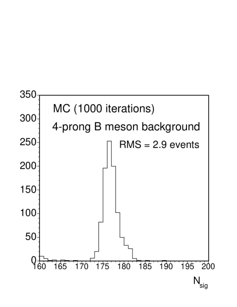
  Figure 8.1: $\Lambda_{b}\rightarrow\Lambda_{c}^{+}\pi^{-}$ yield from 1000 variations of the 4-prong $B$ meson background ${\cal BR}$. The RMS is recorded as the yield change.

Measured Branching Fractions

We use the ${\cal BR}$ from the world average in the PDG to estimate the physics backgrounds in our semileptonic signals as described in Section 7.2. We vary the ${\cal BR}$ of these measured physics backgrounds by $\pm$ 1 $\sigma$. We then calculate $\sigma_{R}$. Note that here the variation of the ${\cal B}(\Lambda_{b}\rightarrow\Lambda_{c}^{+}\pi^{-})$ does not include the uncertainty due to the measured $\Lambda_{b}$ $P_{T}$ spectrum. The $\sigma_{R}$ due to the measured ${\cal BR}$ is 0.43, 0.75 and ${+0.73\atop-2.07}$ for $\overline{B}^{0}\rightarrow D^{*+}$, $\overline{B}^{0}\rightarrow D^{+}$ and $\Lambda_{b}\rightarrow\Lambda_{c}^{+}$ modes, respectively. For the remainder of this section, we quote the systematic uncertainties in the same order.

Unmeasured Branching Fractions

The ${\cal BR}$ of several physics backgrounds in Section 7.2 have not yet been measured, e.g.: $\Lambda_{b}\rightarrow\Lambda_{c}^{+}f^{0}\mu^{-}\overline{\nu}_{\mu}$, or have just been measured by us for this analysis, e.g.:$\Lambda_{b}\rightarrow\Lambda_{c}(2593)^{+}\mu^{-}\overline{\nu}_{\mu}$. For the first case, we use the estimated ${\cal BR}$ from the decay file of EvtGen, and our own derivation based on HQET. As we have no uncertainty input from the estimated ${\cal BR}$, we assign a 5$\%$ uncertainty to the ${\cal BR}$ of the excited charm meson decays and a 100$\%$ uncertainty to the ${\cal BR}$ of the $B$ hadron decays. Because the excited charm hadrons decay via strong interaction and conserve isospin symmetry, their ${\cal BR}$ could be inferred from Clebsch-Gordan Coefficients. While for the weak decays of $B$ hadrons, allowable decay spectrum is wider. For the second case, we add $(20\oplus 20)\%$ uncertainty in quadrature with the uncertainty from the preliminary measurement (see Table 7.5). The first 20$\%$ arises from the unresolved disagreement of measured $\tau_{\Lambda_{b}}$ with that from the HQET prediction. The second 20$\%$ is due to the difference of the soft pion reconstruction efficiency between MC and data. We vary the ${\cal BR}$ by the uncertainties we assigned and calculate the shift of our measurement. The shift due to the unmeasured ${\cal BR}$ is 1.09, 0.91 and 0.50.

Fake $\mu$ estimate

As noted in Section 7.3.1, the systematic uncertainties from the fake $\mu$ estimate originate from:

1. The uncertainty from the fit to the charm mass spectra.

2. The uncertainty on the probabilities for the pions, kaons and protons to fake muons.

3. The uncertainty on the fraction of pion, kaon and proton in the hadron tracks.

For each category, we vary the central value $\pm$ 1 $\sigma$, independently. More detailed description can be found in Section 7.3.1. The resulting uncertainty on the amount of fake muons together with the central value are summarized in Table 8.10.

Table 8.10: Summary of fake muon contamination.

$\overline{B}\rightarrow D^{*+}\mu_{fake}$	$\overline{B}\rightarrow D^{+}\mu_{fake}$	$\overline{B}\rightarrow\Lambda_{c}^{+}\mu_{fake}$
45 $\pm$ 3	230 $\pm$ 19	40 $\pm$ 9

We then vary the number of fake muons $\pm$ 1 $\sigma$ and insert the new number into Equation 8.1. The total variation on $R$ due to the fake $\mu$ estimate is 0.07, 0.07, 0.17.

$b\overline{b}$ and $c\overline{c}$ background

In Section 7.4, we notice a 10–40$\%$ discrepancy of the $D^{0}$, $B^{+}$, and inclusive $b$ cross-section from PYTHIA with those from the data. In addition, we do not possess information about the relative $b\overline{b}$ and $c\overline{c}$ production rates between flavor creation, flavor excitation, and gluon splitting. Therefore, we assign a 100$\%$ uncertainty to the amount of $b\overline{b}$ and $c\overline{c}$ backgrounds. This changes $R$ by 0.22, 0.22, 0.04.

MC sample size

We have generated large MC samples for calculating the efficiencies of our signals and backgrounds, but there is a small statistical uncertainty due to the finite MC sample size. We use the uncertainties on the efficiencies to calculate $\sigma_{R}$. $\sigma_{R}$ is 0.28, 0.18, and 0.32.

MC $P_{T}(B)$ Spectrum

We find discrepancies between data and MC in the $P_{T}$ spectrum of $B^{0}$ and $\Lambda_{b}$, as described in Section 6.1. After reweighting the $P_{T}$ spectrum of $B^{0}$ and $\Lambda_{b}$, we have observed good agreement of MC with the data as seen in Section 6.2. However, there is an uncertainty on the exponential slope of data/MC, $p_{1}$ in Figure 6.2, which is limited by the amount of data used for comparison with the MC. We vary $p_{1}$ $\pm$ 1 $\sigma$ and re-weight the MC events after the analysis cuts numerically to calculate the efficiency change. In addition, we vary the variables which depend on the $\Lambda_{b}$ $P_{T}$ spectrum accordingly, eg: cross-section correction factors and the result of $\frac{\sigma_{\Lambda_{b}}(P_{T}>6.0){\cal B}(\Lambda_{b}\rightarrow\Lambda_{c}^{+}\pi^{-})}{\sigma_{B^{0}}(P_{T}>6.0){\cal B}(\overline{B}^{0}\rightarrow D^{+}\pi^{-})}$ by Le, et al. [68] as described in Section 7.1. The total variation on $R$ due to the MC $P_{T}$ spectrum of $B$ hadrons is 0.38, 0.32, and ${+0.28\atop-0.50}$.

Pion Interaction with the Material

One difference between our semileptonic and hadronic final states is the muon and the pion. The muon does not interact with the material via the hadronic (strong) interaction while the pion does. In order to model the track reconstruction efficiency correctly, two things have to be right:

1. The type and the amount of material in the detector.

2. The model that describes the hadronic interaction cross-section, the final state multiplicities and kinematics.

We generate MC for the signals as described in Section 6.1 except that we switch off the hadronic interaction in the detector simulation. We compare the difference in the hadronic to semileptonic signal efficiency ratio, between the normal MC and the MC with the hadronic interaction off. This difference gives us an idea for the extreme situation, when the material is 100$\%$ wrong. For both the $B^{0}$ and $\Lambda_{b}$ modes, the efficiency ratio changes by 4$\%$. From the study of Korn [102], we know that the available CDF detector simulation underestimate the amount of material by 15$\%$. In addition, a comparison between two programs which model the hadronic interactions, GHEISHA and FLUKA [103], has been done by Michael [104]. The FLUKA package is known to better reproduce the experimental data but currently it is not available in the CDF detector simulation. The effect of the hadronic interaction model estimated by Michael is 20$\%$. Adding 15$\%$ and 20$\%$ in quadrature, we get 25$\%$. We multiply the 100$\%$ efficiency ratio difference described earlier, with 0.25, and get 1$\%$. We apply a scaling factor, 1.01, to all the relative efficiencies, including the semileptonic background to hadronic efficiency ratios. We then re-calculate $R$ and find $\sigma_{R}$ is 0.22, 0.17 and 0.22.

CMU reconstruction efficiency scaling factor

The scaling factor to correct the difference of CMU muon reconstruction efficiency between MC and data has an uncertainty as described in Section 6.3. We vary the scaling factor $\pm$ 1 $\sigma$ and calculate $\sigma_{R}$= 0.07, 0.05, and 0.07.

XFT efficiency scaling factor

We apply the XFT efficiency scaling factors data/MC in bins of inverse $P_{T}$ from Herndon [80] to correct the signal and background efficiencies. The uncertainty on the kaon and pion scaling factors are varied $\pm$ 1 $\sigma$ to evaluate $\sigma_{R}$. For the proton scaling factor, due to the limited statistics, we evaluate the systematic uncertainty following the suggestion in Herndon’s analysis: we compare the difference by applying a constant efficiency scaling factor as shown in Figure 8.2, instead of the one based on the third order polynomial in Figure 6.15. For all the three modes, the systematic uncertainties are negligible as expected, since the final states of our semileptonic and hadronic modes are almost identical and the difference in the ionization of the pion and muon is insignificant. $\sigma_{R}$ is less than 0.01.

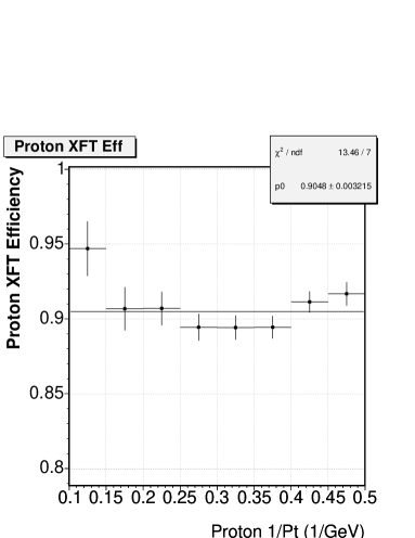
Figure 8.2: The relative proton XFT efficiency between MC and data in bins of 1/$P_{T}$ fit to a constant by Herndon [80].

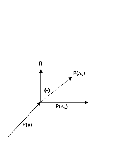
Figure 8.3: Angle definition for the $\Lambda_{b}$ production polarization, where the dashed line indicates the momentum of $\Lambda_{c}$ in the rest frame of $\Lambda_{b}$, and $\mathbf{\hat{n}}$ is the polarization axis normal to the beam proton-$\Lambda_{b}$ production plane.

$\Lambda_{b}$ and $\Lambda_{c}$ polarizations

There is not yet a precise measurement of the production polarizations of $\Lambda_{b}$ and $\Lambda_{c}$, while the Standard Model predicts both particles are produced polarized. The angular distribution of of the $\Lambda_{b}$ daughters is parameterized by

$$\frac{dN}{d\cos\Theta}\propto 1+{\cal P_{B}}\cos\Theta,$$ (8.3)

where ${\cal P_{B}}$ is the product of the $\Lambda_{b}$ polarization and the asymmetry parameter of the weak decay. $\Theta$ is defined as the angle between the $\Lambda_{c}^{+}$ momentum in the $\Lambda_{b}$ rest frame and the axis normal to the beam proton-$\Lambda_{b}$ production plane, $\mathbf{\hat{n}}$. Therefore,

$$\cos\Theta=\mathbf{\hat{P}}(\Lambda_{c})\cdot\mathbf{\hat{n}},$$ (8.4)

where

$$\mathbf{\hat{n}}\equiv\frac{\mathbf{\hat{P}}(p)\times\mathbf{\hat{P}}(\Lambda_{b})}{|\mathbf{\hat{P}}(p)\times\mathbf{\hat{P}}(\Lambda_{b})|},$$ (8.5)

Here “$\times$” (“$\cdot$”) means vector (scalar) product of two vectors. See Figure 8.3 for the definition of $\Theta$ and $\mathbf{\hat{n}}$. The angular distribution of $\Lambda_{c}$ daughters is parameterized in a similar way;

$$\frac{dN}{d\cos\theta}\propto 1+{\cal P_{C}}\cos\theta,$$ (8.6)

where $\theta$ is defined as the angle between the proton momentum in the rest frame of $\Lambda_{c}$ and the $\Lambda_{c}$ momentum in the lab frame, i.e.

$$\cos\Theta=\mathbf{\hat{P}}(\Lambda_{c})\cdot\mathbf{\hat{p}},$$ (8.7)

Note that here $\mathbf{\hat{P}}(\Lambda_{c})$ is in a different frame from that in Equation 8.4. The value of ${\cal P_{B}}$ (${\cal P_{C}}$) is $\pm$ 1 for the polarized state and 0 for the unpolarized state.

The Bgenerator and EvtGen do not include the polarization of $\Lambda_{b}$ and $\Lambda_{c}$. We use the default settings for the central value of $R$. We study the systematics due to a non-null polarization using the generator-level signal MC without the detector and trigger simulation. We use the “acceptance-rejection (Von Neumann)” method [74] and reweight the MC according to:

$$(1+{\cal P_{B}}\cos\Theta)\cdot(1+{\cal P_{C}}\cos\theta),$$

where all combinations of ${\cal P_{B}}$ and ${\cal P_{C}}$ for values at -1, 0, 1 are used. Each MC starts from a different random seed. We apply generator-level analysis-like cuts and obtain the efficiency ratio for each combination. We compare these efficiency ratios with that from the MC generated with zero ${\cal P_{B}}$ and ${\cal P_{C}}$. We find the efficiency ratios are mainly determined by the ${\cal P_{C}}$ as seen in Table 8.11, i.e. the efficiency ratios with the same ${\cal P_{C}}$, but different ${\cal P_{B}}$ are consistent with each other. Therefore, we apply scaling factors from the two ${\cal P_{C}}$ values: -1 and 1 ($\pm$ 1.017$\%$) on all the relative efficiencies and re-calculate $R$. We find $\sigma_{R}$ = 0.37.

Table 8.11: $\epsilon(\Lambda_{b}\rightarrow\Lambda_{c}^{+}\pi^{-})/\epsilon(\Lambda_{b}\rightarrow\Lambda_{c}^{+}\mu^{-}\overline{\nu}_{\mu})$ from each combination of ${\cal P_{B}}$ and ${\cal P_{C}}$.

${\cal P_{B}}$	${\cal P_{C}}$	$\frac{\epsilon(\Lambda_{b}\rightarrow\Lambda_{c}^{+}\pi^{-})}{\epsilon(\Lambda_{b}\rightarrow\Lambda_{c}^{+}\mu^{-}\overline{\nu}_{\mu})}$		Scaling factor
0	0	3.225 $\pm$	0.010	1
0	-1	3.193 $\pm$	0.007	0.990 $\pm$ 0.004
0	1	3.281 $\pm$	0.006	1.017 $\pm$ 0.004
1	0	3.232 $\pm$	0.006	1.002 $\pm$ 0.004
1	-1	3.193 $\pm$	0.009	0.990 $\pm$ 0.004
1	1	3.275 $\pm$	0.009	1.016 $\pm$ 0.004
-1	0	3.235 $\pm$	0.006	1.003 $\pm$ 0.004
-1	1	3.274 $\pm$	0.009	1.015 $\pm$ 0.004
-1	-1	3.175 $\pm$	0.011	0.985 $\pm$ 0.005

$\Lambda_{c}$ Dalitz structure

The $\Lambda_{c}$ from our $\Lambda_{b}\rightarrow\Lambda_{c}^{+}\pi^{-}$ and $\overline{B}\rightarrow\Lambda_{c}^{+}\mu^{-}X$ signal, decays into $p$, $K$, and $\pi$ in the final state. However, any two $\Lambda_{c}$ daughters could form an intermediate resonant state, see Table 8.12. The resonant structure is called the “Dalitz” structure in the literature, and is usually displayed with a Dalitz plot [105], where the invariant mass square of one pair of daughters is plotted versus another pair in the two-dimension. Figure 8.4 (left) shows the Dalitz plot from the $\overline{B}\rightarrow\Lambda_{c}^{+}\mu^{-}X$ data after sideband subtraction. If a resonance exists, a concentrated area near the mass of the resonant particle will be visible. The momenta of $p$, $K$ and $\pi$ are affected by the Dalitz structure and $\Lambda_{b}$ decays have different efficiencies for various structures. However, EvtGen does not take into account the interference of each resonant state. Each state is considered as an independent decay with a ${\cal BR}$ measured by E791 [106] and listed in Table 8.12. See Figure 8.4 (right) for the $\Lambda_{c}$ Dalitz structure in the MC.

Without a better model to describe the $\Lambda_{c}$ Dalitz structure, we study the change in the efficiency ratio of $\Lambda_{b}\rightarrow\Lambda_{c}^{+}\pi^{-}$ to $\Lambda_{b}\rightarrow\Lambda_{c}^{+}\mu^{-}\overline{\nu}_{\mu}$ by varying the ${\cal BR}$ in Table 8.12 $\pm$ 1$\sigma$. We generate four sets of $\Lambda_{b}\rightarrow\Lambda_{c}^{+}\pi^{-}$ and $\Lambda_{b}\rightarrow\Lambda_{c}^{+}\mu^{-}\overline{\nu}_{\mu}$ MC samples without detector and trigger simulation, where $\Lambda_{c}$ decay is forced to one single mode. The efficiency of $\Lambda_{b}$ decay with $\Lambda_{c}^{+}\rightarrow pK^{-}\pi^{+}(\mathrm{total})$, is then the sum of the ${\cal BR}$ weighted efficiency of each individual $\Lambda_{c}$ mode.

$${\cal E}_{c} = \frac{\sum_{i}^{4}{\cal BR}_{i}\cdot\epsilon_{i}}{\sum_{i}^{4}{\cal BR}_{i}},$$ (8.8)

$$R_{c} = \frac{{\cal E}_{c}(\Lambda_{b}\rightarrow\Lambda_{c}^{+}\pi^{-})}{{\cal E}_{c}(\Lambda_{b}\rightarrow\Lambda_{c}^{+}\mu^{-}\overline{\nu}_{\mu})},$$ (8.9)

where ${\cal E}_{c}$ ($R_{c}$) is the total weighted efficiency (ratio) using the central value of each $\Lambda_{c}$ ${\cal BR}$. We re-calculate the absolute and relative efficiency, by varying ${\cal BR}$ of each $\Lambda_{c}$ decay $\pm$ 1 $\sigma$;

$${\cal E}_{j} = \frac{\sum_{i}^{3}{\cal BR}_{i}\cdot\epsilon_{i}+({\cal BR}_{j}+\sigma_{j})\cdot\epsilon_{j}}{\sum_{i}^{4}{\cal BR}_{i}+\sigma_{j}},$$ (8.10)

$$R_{j} = \frac{{\cal E}_{j}(\Lambda_{b}\rightarrow\Lambda_{c}^{+}\pi^{-})}{{\cal E}_{j}(\Lambda_{b}\rightarrow\Lambda_{c}^{+}\mu^{-}\overline{\nu}_{\mu})},$$ (8.11)

where ${\cal E}_{j}$ ($R_{j}$) is the total weighted efficiency (ratio) with ${\cal BR}$ of $j^{th}$ mode varied by $\pm$ 1 $\sigma$ and other ${\cal BR}$ fixed.

We find a fractional change of $0.3\%$ after adding the difference of each $R_{j}$ from $R_{c}$ in quadrature. We apply this fractional change to the relative efficiencies of all the semileptonic backgrounds to the hadronic signal and calculate $\sigma_{R}$= 0.07.

Table 8.12: $\Lambda_{c}$ decays with $p$, $K$, $\pi$ in the final state.

Decay Mode	${\cal BR}(\%)$		$\frac{\epsilon(\Lambda_{b}\rightarrow\Lambda_{c}^{+}\pi^{-})}{\epsilon(\Lambda_{b}\rightarrow\Lambda_{c}^{+}\mu^{-}\overline{\nu}_{\mu})}$		$R_{j}$
$pK^{*}(890)^{0}$	1.6 $\pm$	0.5	3.17 $\pm$	0.01	3.22
$\Delta(1232)^{++}K^{-}$	0.86 $\pm$	0.30	3.24 $\pm$	0.01	3.23
$\Lambda(1520)\pi^{+}$	0.59 $\pm$	0.21	3.30 $\pm$	0.01	3.23
non-resonant	2.8 $\pm$	0.8	3.24 $\pm$	0.01	3.23
$R_{c}$					3.23 $\pm$ 0.01

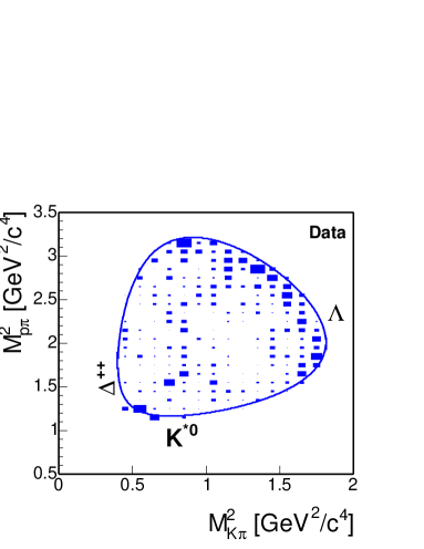
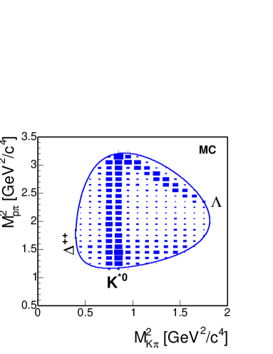
Figure 8.4: $\Lambda_{c}$ Dalitz structure in the sideband subtracted $\overline{B}\rightarrow\Lambda_{c}^{+}\mu^{-}X$ data (left) and MC (right). The concentrated areas in the top figure indicate the existence of $K^{*}(892)^{0}$ and $\Lambda(1520)$. Clearly, the destructive interference between the resonant states are not simulated in the MC.

$\Lambda_{b}$ Lifetime

The world average $\Lambda_{b}$ lifetime is lower than the theoretical prediction. A smaller $\Lambda_{b}$ lifetime gives a smaller efficiency for reconstructing $\Lambda_{b}$ decays. While we cut on the $c\tau$ of $\Lambda_{b}\rightarrow\Lambda_{c}^{+}\pi^{-}$, the $\Lambda_{b}\rightarrow\Lambda_{c}^{+}\mu^{-}\overline{\nu}_{\mu}$ is not fully reconstructed and we actually cut on the pseudo-$c\tau$ of the inclusive semileptonic decays. Therefore, systematics due to the uncertainty on the $\Lambda_{b}$ lifetime may not cancel in our measurement. We study this effect by generating $\Lambda_{b}\rightarrow\Lambda_{c}^{+}\mu^{-}\overline{\nu}_{\mu}$ and $\Lambda_{b}\rightarrow\Lambda_{c}^{+}\pi^{-}$ MC without detector and trigger simulation. We vary the lifetime of $\Lambda_{b}$ $\pm$ 15$\%$ around the central value: 1.229 $ps$. We compare the difference of the relative efficiency ratio from the central value. We then apply a scaling factor from the signals, on the efficiency ratios of the semileptonic backgrounds to the hadronic mode, and calculate $\sigma_{R}$=0.22.

Semileptonic $\Lambda_{b}$ decay model

In Section 6.3, we introduce a scaling factor, $f_{c}$, which accommodates the acceptance difference between the flat phase space MC and the form factor weighted MC. We vary the $f_{c}$ $\pm$ 1 $\sigma$ according to its statistical uncertainty and obtain $\sigma_{R}=\pm 0.57$.

8.1.2 Systematic Uncertainty for Each Mode

Tables 8.13–8.15 list the result of systematic uncertainties as discussed above. The systematics from the external information are separated from the ones from the CDF MC and measurements. Table 8.16 summarizes the uncertainties from each category. The statistical uncertainties on the relative branching fractions are also listed for comparison.

Table 8.13: Statistical and systematic uncertainties of $\frac{{\cal B}(\overline{B}^{0}\rightarrow D^{*+}\mu^{-}\overline{\nu}_{\mu})}{{\cal B}(\overline{B}^{0}\rightarrow D^{*+}\pi^{-})}$.

Source	$\sigma_{R}$
Statistical	$\pm$ $2.3$
Measured ${\cal BR}$
$\overline{B}^{0}\rightarrow D^{*+}\pi^{-}$	$\pm$ 0.29
$B^{-}\rightarrow D_{1}^{0}\mu^{-}\overline{\nu}_{\mu}$	$\pm$ 0.31
$\tau\rightarrow\mu\overline{\nu}_{\mu}\nu_{\tau}$	$<$ 0.01
	$\pm$ 0.43
Unmeasured ${\cal BR}$
$D_{1}^{0}\rightarrow D^{*+}\pi^{-}$	$\pm$ 0.05
$D_{1}^{\prime 0}\rightarrow D^{*+}\pi^{-}$	$\pm$ 0.04
$D_{1}^{+}\rightarrow D^{*+}\pi^{0}$	$\pm$ 0.03
$D_{1}^{\prime+}\rightarrow D^{*+}\pi^{0}$	$\pm$ 0.02
$B^{-}\rightarrow D_{1}^{\prime 0}\mu^{-}\overline{\nu}_{\mu}$	$\pm$ 0.70
$B^{-}\rightarrow D^{*+}\pi^{-}\mu^{-}\overline{\nu}_{\mu}$	$\pm$ 0.39
$\overline{B}^{0}\rightarrow D^{*+}\tau^{-}\overline{\nu}_{\tau}$	$\pm$ 0.31
$\overline{B}^{0}\rightarrow D_{1}^{+}\mu^{-}\overline{\nu}_{\mu}$	$\pm$ 0.53
$\overline{B}^{0}\rightarrow D_{1}^{\prime+}\mu^{-}\overline{\nu}_{\mu}$	$\pm$ 0.34
$\overline{B}^{0}\rightarrow D^{*+}\pi^{0}\mu^{-}\overline{\nu}_{\mu}$	$\pm$ 0.19
	$\pm$ 1.09
CDF Internal Systematics
Fitting of $\overline{B}^{0}\rightarrow D^{*+}\pi^{-}$	$<$ 0.01
Fake $\mu$ estimate	$\pm$ 0.07
$b\overline{b}$ and $c\overline{c}$ background	$\pm$ 0.22
MC sample size	$\pm$ 0.28
MC $P_{T}(B^{0})$	$\pm$ 0.38
$\pi$ interaction with the material	$\pm$ 0.22
CMU reconstruction efficiency scaling factor	$\pm$ 0.07
XFT efficiency scaling factor	$<$ 0.01
	$\pm$ 0.58

Table 8.14: Statistical and systematic uncertainties of $\frac{{\cal B}(\overline{B}^{0}\rightarrow D^{+}\mu^{-}\overline{\nu}_{\mu})}{{\cal B}(\overline{B}^{0}\rightarrow D^{+}\pi^{-})}$.

Source	$\sigma_{R}$
Statistical	$\pm$ $1.0$
Measured ${\cal BR}$
$\overline{B}^{0}\rightarrow D^{+}\pi^{-}$	$\pm$ 0.70
$\overline{B}^{0}\rightarrow D^{*+}\mu^{-}\overline{\nu}_{\mu}$	$\pm$ 0.22
$B^{-}\rightarrow D_{1}^{0}\mu^{-}\overline{\nu}_{\mu}$	$\pm$ 0.08
$D^{*+}\rightarrow D^{+}\pi^{0}$	$\pm$ 0.11
$\tau\rightarrow\mu\overline{\nu}_{\mu}\nu_{\tau}$	$<$ 0.01
$f_{s}/f_{d}$	$\pm$ 0.01
	$\pm$ 0.75
Unmeasured ${\cal BR}$
$D_{1}^{0}\rightarrow D^{*+}\pi^{-}$	$\pm$ 0.01
$D_{1}^{\prime 0}\rightarrow D^{*+}\pi^{-}$	$\pm$ 0.01
$B^{-}\rightarrow D_{1}^{\prime 0}\mu^{-}\overline{\nu}_{\mu}$	$\pm$ 0.17
$B^{-}\rightarrow D^{+}\pi^{-}\mu^{-}\overline{\nu}_{\mu}$	$\pm$ 0.79
$\overline{B}^{0}\rightarrow D^{+}\pi^{0}\mu^{-}\overline{\nu}_{\mu}$	$\pm$ 0.39
$\overline{B}^{0}\rightarrow D^{+}\tau^{-}\overline{\nu}_{\tau}$	$\pm$ 0.10
$\overline{B}_{s}\rightarrow D^{+}K^{0}\mu^{-}\overline{\nu}_{\mu}$	$\pm$ 0.09
	$\pm$ 0.91
CDF Internal Systematics
Fitting of $\overline{B}^{0}\rightarrow D^{+}\pi^{-}$	$\pm$ 0.38
Fitting of $\overline{B}^{0}\rightarrow D^{+}\mu^{-}\overline{\nu}_{\mu}$	$\pm$ 0.13
Fake $\mu$ estimate	$\pm$ 0.07
$b\overline{b}$ and $c\overline{c}$ background	$\pm$ 0.22
MC sample size	$\pm$ 0.18
MC $P_{T}(B^{0})$	$\pm$ 0.32
$\pi$ interaction with the material	$\pm$ 0.17
CMU reconstruction efficiency scaling factor	$\pm$ 0.05
XFT efficiency scaling factor	$<$ 0.01
	$\pm$ 0.62

Table 8.15: Statistical and systematic uncertainties of $\frac{{\cal B}(\Lambda_{b}\rightarrow\Lambda_{c}^{+}\mu^{-}\overline{\nu}_{\mu})}{{\cal B}(\Lambda_{b}\rightarrow\Lambda_{c}^{+}\pi^{-})}$.

Source	$\sigma_{R}$
Statistical	$\pm$ $3.0$
Measured ${\cal BR}$
$\Lambda_{b}\rightarrow\Lambda_{c}^{+}\pi^{-}$	${+0.73\atop-2.07}$
$\tau\rightarrow\mu\overline{\nu}_{\mu}\nu_{\tau}$	$<$ 0.01
Total	${+0.73\atop-2.07}$
Unmeasured ${\cal BR}$
$\Lambda_{b}\rightarrow\Lambda_{c}(2593)^{+}\mu^{-}\overline{\nu}_{\mu}$	$\pm$ 0.21
$\Lambda_{b}\rightarrow\Lambda_{c}(2625)^{+}\mu^{-}\overline{\nu}_{\mu}$	$\pm$ 0.27
$\Lambda_{b}\rightarrow\Sigma_{c}^{0}\pi^{+}\mu^{-}\overline{\nu}_{\mu}$, $\Lambda_{b}\rightarrow\Sigma_{c}^{+}\pi^{0}\mu^{-}\overline{\nu}_{\mu}$, $\Lambda_{b}\rightarrow\Sigma_{c}^{++}\pi^{-}\mu^{-}\overline{\nu}_{\mu}$	$\pm$ 0.24
$\Lambda_{b}\rightarrow\Lambda_{c}^{+}f^{0}\mu^{-}\overline{\nu}_{\mu}$	$\pm$ 0.05
$\Lambda_{b}\rightarrow\Lambda_{c}^{+}\pi^{0}\pi^{0}\mu^{-}\overline{\nu}_{\mu}$, $\Lambda_{b}\rightarrow\Lambda_{c}^{+}\pi^{+}\pi^{-}\mu^{-}\overline{\nu}_{\mu}$	$\pm$ 0.20
$\Lambda_{b}\rightarrow\Lambda_{c}^{+}\tau^{-}\overline{\nu}_{\tau}$	$\pm$ 0.10
$B^{-}\rightarrow\Lambda_{c}^{+}\overline{p}\mu^{-}\overline{\nu}_{\mu}$	$\pm$ 0.11
$\overline{B}^{0}\rightarrow\Lambda_{c}^{+}\overline{n}\mu^{-}\overline{\nu}_{\mu}$	$\pm$ 0.11
Total	$\pm$ 0.50
CDF Internal Systematics
Fitting of $\Lambda_{b}\rightarrow\Lambda_{c}^{+}\pi^{-}$	$\pm$ 0.63
Fake $\mu$ estimate	$\pm$ 0.17
$b\overline{b}$ and $c\overline{c}$ background	$\pm$ 0.04
MC sample size	$\pm$ 0.32
MC $P_{T}(\Lambda_{b})$	${+0.28\atop-0.50}$
$\pi$ interaction with the material	$\pm$ 0.22
CMU reconstruction efficiency scaling factor	$\pm$ 0.07
XFT efficiency scaling factor	$<$ 0.01
$\Lambda_{b}$ and $\Lambda_{c}$ polarizations	$\pm$ 0.37
$\Lambda_{c}^{+}$ Dalitz structure	$\pm$ 0.07
$\Lambda_{b}$ lifetime	$\pm$ 0.22
Semileptonic $\Lambda_{b}$ decay model	$\pm$ 0.57
	${+1.09\atop-1.15}$

Table 8.16: Summary of statistical and systematic uncertainties.

	$\frac{\sigma_{R}}{R}$ ($\%$)
Source	$\frac{{\cal B}(\overline{B}^{0}\rightarrow D^{*+}\mu^{-}\overline{\nu}_{\mu})}{{\cal B}(\overline{B}^{0}\rightarrow D^{*+}\pi^{-})}$	$\frac{{\cal B}(\overline{B}^{0}\rightarrow D^{+}\mu^{-}\overline{\nu}_{\mu})}{{\cal B}(\overline{B}^{0}\rightarrow D^{+}\pi^{-})}$	$\frac{{\cal B}(\Lambda_{b}\rightarrow\Lambda_{c}^{+}\mu^{-}\overline{\nu}_{\mu})}{{\cal B}(\Lambda_{b}\rightarrow\Lambda_{c}^{+}\pi^{-})}$
Measured ${\cal BR}$ ($\%$)	2.4	7.7	${+3.5\atop-10.5}$
Unmeasured ${\cal BR}$ ($\%$)	6.2	9.3	2.5
CDF internal ($\%$)	3.3	6.4	6.0
Statistical ($\%$)	13.1	10.2	15.0

8.1.3 Consistency Check of $R$

In order to detect any unexpected systematics in $R$, we separate the data and MC into several groups of independent subsets according to the run number, vertex position, $c\tau$ and $P_{T}$ of the charm and $B$ hadrons, and etc. We cross-check the consistency of the $R$ within each group. Figure 8.5 displays the result of the cross-check, where the uncertainties in the figure are statistical only. The $R$ from all the subsets are consistent with the other subsets in the same group.

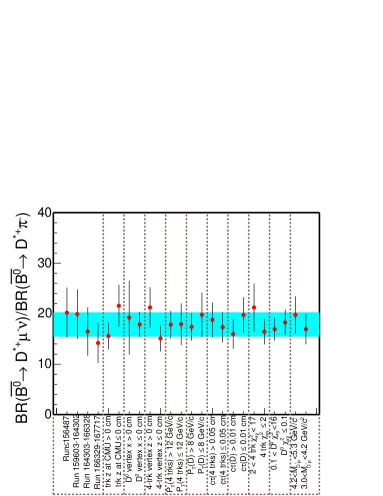
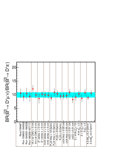
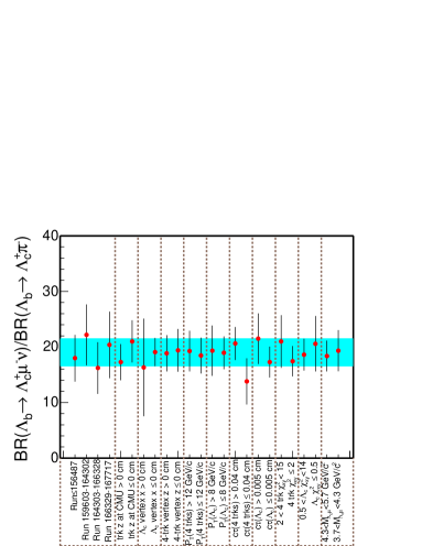
Figure 8.5: Consistency check of ${\cal B}(\overline{B}^{0}\rightarrow D^{*+}\mu^{-}\overline{\nu}_{\mu})/{\cal B}(\overline{B}^{0}\rightarrow D^{*+}\pi^{-})$ (top left), ${\cal B}(\overline{B}^{0}\rightarrow D^{+}\mu^{-}\overline{\nu}_{\mu})/{\cal B}(\overline{B}^{0}\rightarrow D^{+}\pi^{-})$ (top right) and ${\cal B}(\Lambda_{b}\rightarrow\Lambda_{c}^{+}\mu^{-}\overline{\nu}_{\mu})/{\cal B}(\Lambda_{b}\rightarrow\Lambda_{c}^{+}\pi^{-})$ (bottom). The uncertainty on each point is statistical only. Each independent group is separated by a vertical dashed line.

8.2 Measurement Result

For the control modes, we measure the relative branching fractions to be:

$$\frac{{\cal B}(\overline{B}^{0}\rightarrow D^{*+}\mu^{-}\overline{\nu}_{\mu})}{{\cal B}(\overline{B}^{0}\rightarrow D^{*+}\pi^{-})}=17.7\ \pm 2.3\ (stat)\pm 0.6\ (syst)\pm 0.4\ (BR)\pm 1.1\ (UBR),$$

and

$$\frac{{\cal B}(\overline{B}^{0}\rightarrow D^{+}\mu^{-}\overline{\nu}_{\mu})}{{\cal B}(\overline{B}^{0}\rightarrow D^{+}\pi^{-})}=9.8\ \pm 1.0\ (stat)\pm 0.6\ (syst)\pm 0.8\ (BR)\pm 0.9\ (UBR),$$

which are consistent with the ratios obtained by the PDG, $19.7\pm 1.7$ and $7.8\pm 1.0$ at the 0.7 and 1.1 $\sigma$ level. Finally, we measure the relative $\Lambda_{b}$ branching fraction to be:

$$\frac{{\cal B}(\Lambda_{b}\rightarrow\Lambda_{c}^{+}\mu^{-}\overline{\nu}_{\mu})}{{\cal B}(\Lambda_{b}\rightarrow\Lambda_{c}^{+}\pi^{-})}=20.0\ \pm 3.0\ (stat)\pm 1.2\ (syst){+0.7\atop-2.1}\ (BR)\pm 0.5\ (UBR).$$

The uncertainties of the relative branching fractions are from statistics, CDF internal systematics, external measured branching ratios and unmeasured branching ratios, respectively.

8.3 Estimate of the ${\cal B}(\Lambda_{b}\rightarrow\Lambda_{c}^{+}\mu^{-}\overline{\nu}_{\mu})$

We have just presented the first measurement of the ratio of $\Lambda_{b}$ exclusive semileptonic to hadronic branching fractions. The ratio provides important input for the absolute branching fraction of $\Lambda_{b}\rightarrow\Lambda_{c}^{+}\mu^{-}\overline{\nu}_{\mu}$ or $\Lambda_{b}\rightarrow\Lambda_{c}^{+}\pi^{-}$. Leibovich et al. [33] predict ${\cal B}(\Lambda_{b}\rightarrow\Lambda_{c}^{+}\pi^{-})$ = 0.45$\%$ and ${\cal B}(\Lambda_{b}\rightarrow\Lambda_{c}^{+}\mu^{-}\overline{\nu}_{\mu})$ = 6.6$\%$, which gives a relative branching fraction of 14.7. However, the largest theoretical uncertainty from the functional form of the Isgur-Wise function is 30$\%$, due to the assumption of the large $N_{c}$ limit (see Section 2.3). Our measurement of the ratio has a $19\%$ uncertainty and may stimulate additional theoretical work. Multiplying our $\Lambda_{b}$ relative branching fraction, with our derivation of ${\cal B}(\Lambda_{b}\rightarrow\Lambda_{c}^{+}\pi^{-})$ from the CDF measurement of $\frac{\sigma_{\Lambda_{b}}(P_{T}>6.0){\cal B}(\Lambda_{b}\rightarrow\Lambda_{c}^{+}\pi^{-})}{\sigma_{B^{0}}(P_{T}>6.0){\cal B}(\overline{B}^{0}\rightarrow D^{+}\pi^{-})}$ [68] in Section 7.1:

$${\cal B}(\Lambda_{b}\rightarrow\Lambda_{c}^{+}\pi^{-})=\left(0.41\pm 0.19\ (stat\oplus syst){+0.06\atop-0.08}\ ({\it P_{T}})\right)\%,$$

we obtain

$${\cal B}(\Lambda_{b}\rightarrow\Lambda_{c}^{+}\mu^{-}\overline{\nu}_{\mu})=\left(8.1\ \pm 1.2\ (stat){+1.1\atop-1.6}\ (syst)\pm 4.3\ ({\cal B}(\Lambda_{b}\rightarrow\Lambda_{c}^{+}\pi^{-}))\right)\%.$$

which is also consistent with a recent DELPHI result derived from the $\Lambda_{b}\rightarrow\Lambda_{c}^{+}\mu^{-}\overline{\nu}_{\mu}$ form factor measurement [37],

$${\cal B}(\Lambda_{b}\rightarrow\Lambda_{c}^{+}\mu^{-}\overline{\nu}_{\mu})^{\mathrm{DELPHI}}=\left(5.0{+1.1\atop-0.9}(stat){+1.6\atop-1.2}(syst)\right)\%$$

Combining our and DELPHI’s numbers, we obtain $\left(5.5\pm 1.8(stat\oplus syst)\right)\%$. Our relative branching ratios and the derived ${\cal B}(\Lambda_{b}\rightarrow\Lambda_{c}^{+}\pi^{-})$, ${\cal B}(\Lambda_{b}\rightarrow\Lambda_{c}^{+}\mu^{-}\overline{\nu}_{\mu})$ are all in agreement with the predictions by Leibovich et al., within large uncertainties. Note that the dominant uncertainties of ${\cal B}(\Lambda_{b}\rightarrow\Lambda_{c}^{+}\pi^{-})$ arise from $\frac{\sigma_{\Lambda_{b}}}{\sigma_{B^{0}}}$ and ${\cal B}(\Lambda_{c}^{+}\rightarrow pK^{-}\pi^{+})$. New CDF-II measurements of $\frac{\sigma_{\Lambda_{b}}}{\sigma_{B^{0}}}$ are anticipated. However, a better measurement of ${\cal B}(\Lambda_{c}^{+}\rightarrow pK^{-}\pi^{+})$ has only been proposed by Dunietz [107] and Migliozzi [108]. Improvements in the ${\cal B}(\Lambda_{b}\rightarrow\Lambda_{c}^{+}\pi^{-})$ will reduce the uncertainties in our determination of the exclusive semileptonic branching ratio.

8.4 Conclusion

We analyze 171.5 $\mathrm{pb^{-1}}$ of data collected with the CDF-II detector in the $p\overline{p}$ collisions at $\sqrt{s}=1.96\rm~{}TeV$. Using a novel secondary vertex track trigger, we reconstruct $1237\ \pm 97$ $\overline{B}\rightarrow\Lambda_{c}^{+}\mu^{-}X$ decays and $179\ \pm 19$ $\Lambda_{b}\rightarrow\Lambda_{c}^{+}\pi^{-}$ decays. This is the largest $\Lambda_{b}$ sample in the world, which enables us to measure the relative $\Lambda_{b}$ branching fractions and examine the Heavy Quark Effective Theory. We have also observed several $\Lambda_{b}$ semileptonic decays which have never been seen in the other experiments: $\Lambda_{b}\rightarrow\Lambda_{c}(2593)^{+}\mu^{-}X$, $\Lambda_{b}\rightarrow\Lambda_{c}(2625)^{+}\mu^{-}X$, $\Lambda_{b}\rightarrow\Sigma_{c}^{0}\pi^{+}\mu^{-}X$, and $\Lambda_{b}\rightarrow\Sigma_{c}^{++}\pi^{-}\mu^{-}X$. In addition, we reconstruct the $\overline{B}^{0}\rightarrow D^{*+}$ and $\overline{B}^{0}\rightarrow D^{+}$ decays similar to our $\Lambda_{b}$ decays and use them as the control samples to understand the issues associated with the $\Lambda_{b}$ measurement. After the estimate and the subtraction of the background in the inclusive semileptonic signal, we correct the yield observed in the data with the trigger and reconstruction efficiencies obtained from the Monte Carlo. We find the relative branching fraction of the control modes in good agreement with the values obtained by the PDG. We measure the ratio of $\Lambda_{b}$ branching fraction to be:

$$\frac{{\cal B}(\Lambda_{b}\rightarrow\Lambda_{c}^{+}\mu^{-}\overline{\nu}_{\mu})}{{\cal B}(\Lambda_{b}\rightarrow\Lambda_{c}^{+}\pi^{-})}=20.0\pm 3.0(stat)\pm 1.2(syst){+0.7\atop-2.1}(BR)\pm 0.5(UBR).$$

The uncertainty is dominated by the size of the data sample and the branching ratio of $\Lambda_{b}\rightarrow\Lambda_{c}^{+}\pi^{-}$. More data and a more precise measurement of ${\cal B}(\Lambda_{b}\rightarrow\Lambda_{c}^{+}\pi^{-})$ in the future will immediately improve our relative branching fraction measurement and our determination of ${\cal B}(\Lambda_{b}\rightarrow\Lambda_{c}^{+}\mu^{-}\overline{\nu}_{\mu})$.

8.5 Future

In addition to the measurement presented in this dissertation, several measurements can be performed at CDF and increase our knowledge of the $\Lambda_{b}$.

$\Lambda_{b}$ lifetime

Previous analyses [7, 109, 110, 111] used semileptonic decays to measure the $\Lambda_{b}$ lifetime so the $\Lambda_{b}$ was not fully reconstructed. A scaling factor based on the MC was applied to convert the total momenta of the observed daughters to the $\Lambda_{b}$ parent momentum. On top of that, possible backgrounds from the other $\Lambda_{b}$ decays might not have been included. Therefore, a $\Lambda_{b}$ lifetime measurement using fully reconstructed decays, such as $\Lambda_{b}\rightarrow\Lambda_{c}^{+}\pi^{-}$ or $\Lambda_{b}\rightarrow J/\Psi\Lambda$, can provide a model-independent comparison with the current world average and the theoretical prediction and possibly resolve the discrepancy as noted in Chapter 1.

$\Lambda_{b}$ production cross-section

Instead of measuring the ratio of two branching fractions, we can measure an absolute branching ratio directly if the $\Lambda_{b}$ production cross-section at the Tevatron is known. An alternative way is to measure the ratio of the $\Lambda_{b}$ to $B^{0}$ production cross-section. As noted in Section 8.3, an accurate measurement of the $\frac{\sigma_{\Lambda_{b}}}{\sigma_{B^{0}}}$ will reduce the uncertainty on the ${\cal B}(\Lambda_{b}\rightarrow\Lambda_{c}^{+}\pi^{-})$ when normalizing the $\Lambda_{b}$ decays to the $B$ meson decays.

$\Lambda_{b}\rightarrow\Lambda_{c}^{+}\mu^{-}\overline{\nu}_{\mu}$ form factor and $|V_{cb}|$

As the three-dimensional (3D) vertex reconstruction using the SVX information is not fully developed at CDF-II, yet, this analysis made requirements only on the two-dimensional vertex ($L_{xy}$) when reconstructing $\Lambda_{c}\mu$ events. Once the 3D vertex reconstruction is mature, we can use kinematic constraints to obtain the neutrino momentum and calculate the scalar product of the $\Lambda_{b}$ and the $\Lambda_{c}$ four-velocities, $w$. The $w$ distribution can be fit to the Isgur-Wise function to obtain the slope parameter, $\rho^{2}$, in Equation 2.34. When an exact form of the Isgur-Wise function is established, the $\Lambda_{b}$ semileptonic decays can give a $|V_{cb}|$ competitive with that from the $B$ meson decays [112, 113].

CP asymmetry in the $\Lambda_{b}\rightarrow p\pi$ and $\Lambda_{b}\rightarrow pK$ decays

Bensalem, et al. [114] and Dunietz [115] predict a large T violation (or CP asymmetry) in the charmless $\Lambda_{b}$ decays in the Standard Model. The asymmetry can be studied without a need for the flavor tagging since the baryon decays are not affected by the mixing. However, $\Lambda_{b}$ charmless decays, such as $\Lambda_{b}\rightarrow p\pi$ and $\Lambda_{b}\rightarrow pK$, have not been observed, yet. A recent search for these decays at CDF-II by Carosi, et al. [116] set an upper limit on the branching fraction ${\cal B}(\Lambda_{b}\rightarrow ph)\leq 23\cdot 10^{-6}$ at 90$\%$ confidence level, and improved the previous upper limit by ALEPH [117]. More data in the future can either improve the upper limit or result a first observation of the signal. Once enough signal is established, a CP asymmetry measurement can be made.

Bibliography

- [1] C. Albajar et al. (UA1), Phys. Lett. B273, 540 (1991).
- [2] P. Abreu et al. (DELPHI), Phys. Lett. B374, 351 (1996).
- [3] D. Buskulic et al. (ALEPH), Phys. Lett. B380, 442 (1996).
- [4] F. Abe et al. (CDF), Phys. Rev. D55, 1142 (1997).
- [5] Andreas Korn, Measurement of the B Hadron Masses in exclusive Decay Channels, CDF Internal Note CDF/ANAL/BOTTOM/CDFR/6963, Massachusetts Institute of Technology (2004).
- [6] P. Abreu et al. (DELPHI), Z. Phys. C68, 375 (1995).
- [7] R. Barate et al. (ALEPH), Eur. Phys. J. C2, 197 (1998).
- [8] S. Eidelman et al. (Particle Data Group), Phys. Lett. B592, 1 (2004).
- [9] K. Anikeev et al. (2001), hep-ph/0201071.
- [10] S. Weinberg, The Quantum theory of fields. Vol. 1–3: Foundations (Cambridge, UK: Univ. Pr., 1995,1996,2000).
- [11] M. E. Peskin and D. V. Schroeder, An Introduction to quantum field theory (Reading, USA: Addison-Wesley, 1995).
- [12] R. G. H. Robertson, Nucl. Phys. Proc. Suppl. 138, 243 (2005).
- [13] P. Wittich, First Measurement of the Flux of Solar Neutrinos, SNO Thesis, University of Pennsylvania (2000).
- [14] Y. Ashie et al. (Super-Kamiokande) (2005), hep-ex/0501064.
- [15] P. J. Litchfield (Soudan 2), Nucl. Phys. Proc. Suppl. 138, 402 (2005).
- [16] M. Ambrosio et al. (MACRO), Eur. Phys. J. C36, 323 (2004).
- [17] G. L. Kane, Modern Elementary Particle Physics (Reading, USA: Addison-Wesley, 1987).
- [18] N. Cabibbo, Phys. Rev. Lett. 10, 531 (1963).
- [19] M. Kobayashi and T. Maskawa, Prog. Theor. Phys. 49, 652 (1973).
- [20] L.-L. Chau and W.-Y. Keung, Phys. Rev. Lett. 53, 1802 (1984).
- [21] H. Harari and M. Leurer, Phys. Lett. B181, 123 (1986).
- [22] H. Fritzsch and J. Plankl, Phys. Rev. D35, 1732 (1987).
- [23] F. J. Botella and L.-L. Chau, Phys. Lett. B168, 97 (1986).
- [24] Nucl. Instrum. Meth. A479, 117 (2002).
- [25] D. Boutigny et al. (BABAR) SLAC-R-0457.
- [26] K. Arisaka et al. FERMILAB-FN-0580.
- [27] K. G. Wilson, Phys. Rev. 179, 1499 (1969).
- [28] U. Aglietti, Phys. Lett. B281, 341 (1992).
- [29] A. V. Manohar and M. B. Wise, Heavy quark physics (Camb. Monogr. Part. Phys. Nucl. Phys. Cosmol., 2000).
- [30] S. Godfrey and N. Isgur, Phys. Rev. D32, 189 (1985).
- [31] N. Isgur and M. B. Wise, Phys. Lett. B237, 527 (1990).
- [32] H. Georgi, B. Grinstein, and M. B. Wise, Phys. Lett. B252, 456 (1990).
- [33] A. K. Leibovich, Z. Ligeti, I. W. Stewart, and M. B. Wise, Phys. Lett. B586, 337 (2004), hep-ph/0312319.
- [34] N. Isgur and M. B. Wise, Phys. Lett. B232, 113 (1989).
- [35] E. Jenkins, A. V. Manohar, and M. B. Wise, Nucl. Phys. B396, 38 (1993), hep-ph/9208248.
- [36] M.-Q. Huang, H.-Y. Jin, J. G. Korner, and C. Liu (2005), hep-ph/0502004.
- [37] J. Abdallah et al. (DELPHI), Phys. Lett. B585, 63 (2004), hep-ex/0403040.
- [38] G. Aubrecht et al., Contemporary Physics Education Project (2003), http://www.lbl.gov/abc/wallchart/teachersguide/pdf/Chap11.pdf.
- [39] C. W. Schmidt Presented at 1993 Particle Accelerator Conference (PAC 93), Washington, DC, 17-20 May 1993.
- [40] Ferrmilab Beam Division http://www-bd.fnal.gov/runII/index.html.
- [41] D. Acosta et al. (CDF), Phys. Rev. D71, 032001 (2005), hep-ex/0412071.
- [42] A. Affolder et al. (CDF), Nucl. Instrum. Meth. A453, 84 (2000).
- [43] C. S. Hill (On behalf of the CDF), Nucl. Instrum. Meth. A530, 1 (2004).
- [44] D. Acosta et al. (CDF-II), Nucl. Instrum. Meth. A518, 605 (2004).
- [45] L. Balka et al. (CDF), Nucl. Instrum. Meth. A267, 272 (1988).
- [46] S. Bertolucci et al. (CDF), Nucl. Instrum. Meth. A267, 301 (1988).
- [47] S. Kuhlmann et al., Nucl. Instrum. Meth. A518, 39 (2004), physics/0310155.
- [48] A. Artikov et al., Nucl. Instrum. Meth. A538, 358 (2005), physics/0403079.
- [49] D. Acosta et al. (CDF), Nucl. Instrum. Meth. A461, 540 (2001).
- [50] D. Acosta et al., Nucl. Instrum. Meth. A494, 57 (2002).
- [51] G. F. Knoll, Radiation Detection and Measurement (New York, USA: John Wiley Sons (2000) 816 p, 2000).
- [52] R. Veenhof, Nucl. Instrum. Meth. A419, 726 (1998).
- [53] W. Bokhari, F. M. Newcomer, et al., The ASDQ ASIC, CDF Internal Note CDF/DOC/TRACKING/CDFR/4515, University of Pennsylvania, Fermilab (1998).
- [54] Shin-Shan Yu, Joel Heinrich, Nigel Lockyer, et al., COT Measurement and Corrections, CDF Internal Note CDF/DOC/BOTTOM/PUBLIC/6361, University of Pennsylvania (2003).
- [55] M. Donega, S. Giagu, D. Tonelli, et al., Track-based calibration of the COT specific ionization, CDF Internal Note CDF/ANAL/BOTTOM/CDFR/6932, INFN, Rome, Pisa, and University of Geneva (2004).
- [56] C. Hays, P. Tamburello, et al., The COT Pattern Recognition Algorithm and Offline Code, CDF Internal Note CDF/DOC/TRACKING/CDFR/6992, Duke University, Fermilab and University of Pennsylvania (2004).
- [57] G. Ascoli et al., Nucl. Instrum. Meth. A268, 33 (1988).
- [58] P. T. Lukens (CDF IIb) FERMILAB-TM-2198.
- [59] E. J. Thomson et al., IEEE Trans. Nucl. Sci. 49, 1063 (2002).
- [60] B. Ashmanskas et al. (CDF-II), Nucl. Instrum. Meth. A518, 532 (2004), physics/0306169.
- [61] G. Gomez-Ceballos et al., Nucl. Instrum. Meth. A518, 522 (2004).
- [62] D. Lucchesi et al., Study of Yields in the Hadronic Trigger, CDF Internal Note CDF/PHYS/BOTTOM/CDFR/6345, INFN, Padova (2003).
- [63] J. Marriner, Secondary Vertex Fit with Mass and Pointing Constraints (CTVMFT), Tech. Rep. CDF/DOC/SECVTX/PUBLIC/1996 (1993).
- [64] S.-S. Yu, R. Tesarek, N. Lockyer, and D. Litvintsev, Description of the Datasets for the Ratio of Semileptonic to Hadronic Partial Decay Width, CDF Internal Note CDF/PHYS/BOTTOM/CDFR/6979, University of Pennsylvania,Fermilab (2004).
- [65] S.-S. Yu, R. Tesarek, D. Litvintsev, J. Heinrich, and N. Lockyer, Ratio of Semileptonic to Hadronic Branching Fractions in the Two Track Trigger, CDF Internal Note CDF/PHYS/BOTTOM/CDFR/7559, University of Pennsylvania,Fermilab (2005).
- [66] F. James and M. Roos, Comput. Phys. Commun. 10, 343 (1975).
- [67] I. Furic, Measurement of the Ratio of Branching Fractions at CDF-II, CDF Thesis CDF/THESIS/BOTTOM/PUBLIC/7352, Massachusetts Institute of Technology (2004).
- [68] Y. Le, M. Martin, and P. Maksimović, Observation of and the Measurement of , CDF Internal Note CDF/ANAL/BOTTOM/CDFR/6396, Johns Hopkins University (2004).
- [69] A. Belloni, J. Piedra et al., Unbinned Likelihood Fit for B0 Mixing in Fully Reconstructed Decays, CDF Internal Note CDF/PHYS/BOTTOM/CDFR/7388 (2004), see Chapter 11.
- [70] K. Anikeev, P. Murat, and C. Paus, Description of Bgenerator, CDF Internal Note CDF/DOC/BOTTOM/CDFR/5092, MIT (1999).
- [71] T. Sjostrand, L. Lonnblad, and S. Mrenna (2001), hep-ph/0108264.
- [72] P. Nason, S. Dawson, and R. K. Ellis, Nucl. Phys. B327, 49 (1989).
- [73] C. Peterson, D. Schlatter, I. Schmitt, and P. M. Zerwas, Phys. Rev. D27, 105 (1983).
- [74] C. Caso et al., Phys. Let. B (2004), see Monte Carlo techniques, page 289.
- [75] D. J. Lange, Nucl. Instrum. Meth. A462, 152 (2001).
- [76] R. Brun, R. Hagelberg, M. Hansroul, and J. C. Lassalle CERN-DD-78-2-REV.
- [77] J. Heinrich, Private communications.
- [78] Ken Bloom and David Dagenhart, Muon-Reconstruction Efficiency for Winter 2003 Conferences, CDF Internal Note CDF/ANAL/MUON/CDFR/6347 (2003).
- [79] S.Giagu, M.Rescigno, et al.., BR ratios and direct CP violation in Cabibbo supressed decays of , CDF Internal Note CDF/PHYS/BOTTOM/CDFR/6391 (2003).
- [80] M. Herndon, et al.., Proton XFT Efficiency Estimate for Analysis, CDF Internal Note CDF/PHYS/BOTTOM/CDFR/7301 (2004).
- [81] T. Yamashita and e. Ting Miao, Measurement of , CDF Internal Note CDF/PHYS/BOTTOM/CDFR/6643, Okayama University, Fermilab and Argonne National Laboratory (2003).
- [82] D. Abbaneo et al. (ALEPH) (2001), hep-ex/0112028.
- [83] T. Affolder et al. (CDF), Phys. Rev. Lett. 84, 1663 (2000), hep-ex/9909011.
- [84] W. Taylor, A Measurement of b-quark Fragmentation Fractions in Collisions at = 1.8 TeV, CDF Thesis CDF/THESIS/BOTTOM/PUBLIC/4913, University of Toronto (1999).
- [85] Avery, P. and Read, K. and Trahern, G., QQ: A Monte Carlo Generator, CLEO Software Note CSN-212 (1985).
- [86] D. Litvintsev, S.-S. Yu, and R. Tesarek, Observation of and in semileptonic decays, CDF Internal Note CDF/PHYS/BOTTOM/CDFR/7546, Fermilab, University of Pennsylvania (2005).
- [87] R. Tesarek and S.-S. Yu, A Study of Backgrounds to the Decay , CDF Internal Note CDF/PHYS/BOTTOM/CDFR/6599, Fermilab, University of Pennsylvania (2003).
- [88] R. Tesarek, S.-S. Yu, and D. Litvintsev, A Study of Backgrounds to the decay , CDF Internal Note CDF/ANAL/BOTTOM/CDFR/7545, Fermilab, University of Pennsylvania (2005).
- [89] K. W. Edwards et al. (CLEO), Phys. Rev. Lett. 74, 3331 (1995).
- [90] H. Albrecht et al. (ARGUS), Phys. Lett. B402, 207 (1997).
- [91] A. K. Leibovich and I. W. Stewart, Phys. Rev. D57, 5620 (1998), hep-ph/9711257.
- [92] CDF Collaboration, Phys. Rev. D 68, 091101 (2003).
- [93] D. Litvintsev, CDF note in preparation, Tech. Rep.
- [94] D. Acosta et al. (CDF II) (2004), hep-ex/0406078.
- [95] K. Lannon and K. Pitts, Bottom Quark Production Using PYTHIA and HERWIG, CDF Internal Note CDF/PHYS/BOTTOM/CDFR/6253, University of Illinois at Urbana-Champaign (2003).
- [96] R. Field, The Sources of b-quarks at the Tevatron, CDF Internal Note CDF/ANAL/BOTTOM/CDFR/5558, University of Florida (2001).
- [97] G. Gomez-Ceballos et al., B Monte Carlo homepage, Tech. Rep. (2004), see http://www-cdf.fnal.gov/internal/physics/bottom/b-montecarlo/db/g020.txt.
- [98] CDF Collaboration, Phys. Rev. D 65, 052006 (2002).
- [99] D. Acosta et al. (CDF), Phys. Rev. Lett. 91, 241804 (2003), hep-ex/0307080.
- [100] D. Acosta et al. (CDF), Measurements of bottom anti-bottom azimuthal production correlations in proton antiproton collisions at s**(1/2) = 1.8-TeV, Tech. Rep. (2004), hep-ex/0412006.
- [101] M. Martin et al., Evaluation of fit systematics due to background shapes in , Tech. Rep. CDF/DOC/BOTTOM/PUBLIC/6953, Johns Hopkins University (2004).
- [102] A. Korn, G. Bauer and C. Paus, Update on Calibration of Energy Loss and Magnetic Field using Events in Run II, CDF Internal Note CDF/DOC/BOTTOM/CDFR/6355, Massachusetts Institute of Technology (2003).
- [103] R. Brun, F. Bruyant, M. Maire, A. C. McPherson, and P. Zanarini CERN-DD/EE/84-1.
- [104] D. Michael (1994), nuMI-NOTE-BEAM-0019.
- [105] R. H. Dalitz, Phil. Mag. 44, 1068 (1953).
- [106] E. M. Aitala et al. (E791), Phys. Lett. B471, 449 (2000), hep-ex/9912003.
- [107] I. Dunietz, Phys. Rev. D58, 094010 (1998), hep-ph/9805287.
- [108] P. Migliozzi, G. D’Ambrosio, G. Miele, and P. Santorelli (CHORUS), Phys. Lett. B462, 217 (1999), hep-ph/9906219.
- [109] P. Abreu et al. (DELPHI), Eur. Phys. J. C10, 185 (1999).
- [110] K. Ackerstaff et al. (OPAL), Phys. Lett. B426, 161 (1998), hep-ex/9802002.
- [111] F. Abe et al. (CDF), Phys. Rev. Lett. 77, 1439 (1996).
- [112] N. Isgur and M. B. Wise, Nucl. Phys. B348, 276 (1991).
- [113] H. Georgi, Nucl. Phys. B348, 293 (1991).
- [114] W. Bensalem, A. Datta, and D. London, Phys. Lett. B538, 309 (2002), hep-ph/0205009.
- [115] I. Dunietz, Z. Phys. C56, 129 (1992).
- [116] R. Carosi and M. A. Ciocci and S. Torre, Search for and decays, CDF Internal Note CDF/PUB/BOTTOM/PUBLIC/7443, INFN, Sez di Pisa (2005), See http://fcdfwww.fnal.gov/internal/physics/godparents/lbppipk/.
- [117] D. Buskulic et al. (ALEPH), Phys. Lett. B384, 471 (1996).