${\it K}^{0}_{s}$ and $\Lambda^{0}$ Production Studies in $p\bar{p}$ Collisions at $\sqrt{s}$ = 1800 and 630 GeV

Abstract

We present a study of the production of ${\it K}^{0}_{s}$ and $\Lambda^{0}$ in inelastic $p\bar{p}$ collisions at $\sqrt{s}$= 1800 and 630 GeV using data collected by the CDF experiment at the Fermilab Tevatron. Analyses of ${\it K}^{0}_{s}$ and $\Lambda^{0}$ multiplicity and transverse momentum distributions, as well as of the dependencies of the average number and $\langle p_{T}\rangle$ of ${\it K}^{0}_{s}$ and $\Lambda^{0}$ on charged particle multiplicity are reported. Systematic comparisons are performed for the full sample of inelastic collisions, and for the low and high momentum transfer subsamples, at the two energies. The $p_{T}$ distributions extend above 8 GeV/c, showing a $\langle p_{T}\rangle$ higher than previous measurements. The dependence of the mean ${\it K}^{0}_{s}(\Lambda^{0})$ $p_{T}$ on the charged particle multiplicity for the three samples shows a behavior analogous to that of charged primary tracks.

I INTRODUCTION

Hadron interactions are often classified as either “hard” or “soft” ua2 ; sjo . Although there is no formal definition for either, the term “hard interactions” denotes high momentum transfer parton-parton interactions typically associated with such phenomena as jets of high energy transverse to the incoming hadron momenta ($E_{T}$). The “soft” interaction component encompasses everything else and dominates the inelastic cross-section. From a theoretical point of view, perturbative QCD provides a reasonable description of high-$E_{T}$ jet production. However, non-perturbative QCD, relevant to low-$E_{T}$ hadronic production, is not well understood. Some QCD-inspired models sjo attempt to describe these processes by the superposition of many parton interactions extrapolated to very low momentum transfers. It is not known, however, if these or other collective multi-parton processes are at work. The experimental studies of low-$E_{T}$ interactions are usually performed on data collected using minimum bias (MB) triggers, which, ideally, sample events in fixed proportion to the production rate — in other words, in their “natural” distribution. Lacking a comprehensive description of the microscopic processes mod involved in low-$E_{T}$ interactions, our knowledge of the details of low transverse momentum ($p_{T}$) particle production rests largely upon empirical connections between phenomenological models and data collected with MB triggers at many center-of-mass energies ($E_{cms}$). Such comparisons necessarily face the difficulty of isolating events of a purely “soft” or “hard” nature.

Comparative studies of the event structure through collective variables such as the charged particle multiplicity and the transverse energy of the event are important to our understanding of the soft production mechanism. In a previous paper noi , a novel approach in addressing this issue using samples of $p\bar{p}$ collisions at $\sqrt{s}=1800$ and 630 GeV collected with an MB trigger was described. The analysis divided the full MB samples into two subsamples, one highly enriched in soft interactions, the other in hard interactions. Comparisons between the subsamples and as a function of $E_{cms}$ were performed. The same approach has been applied here to the production of strange particles.

Beside gluons and the lighter quarks u and d, strange quark production is the only component of low-$p_{T}$ multiparticle interactions which is statistically significant and experimentally accessible with an MB trigger. It is also a probe for investigating the transition of soft hadron interactions to the QCD high-$p_{T}$ perturbative region.

This paper describes a study of ${\it K}^{0}_{s}$ and $\Lambda^{0}$ production in $p\bar{p}$ interactions at different $E_{cms}$. Inclusive distributions of the multiplicity and transverse momentum of ${\it K}^{0}_{s}$ and $\Lambda^{0}$ are presented first. The high statistics of the data sample collected at $\sqrt{s}$= 1800 and 630 GeV allow an extension of the range and precision of these measurements with respect to previous ones. Studies of the dependence of the average $p_{T}$ of ${\it K}^{0}_{s}(\Lambda^{0})$ and of their mean number on the event charged multiplicity are also presented. Different behavior of the hard and soft subsamples is observed, consistent with prior reports on charged particles noi .

II DATA COLLECTION

II.1 The CDF Detector

Data samples have been collected with the CDF detector at the Fermilab Tevatron Collider. The CDF apparatus has been described elsewhere detec ; here only the parts of the detector utilized for the present analysis are discussed. The coordinate system is defined with respect to the proton beam direction, which defines the positive $z$ direction, while the azimuthal angle $\phi$ is measured around the beam axis. The polar angle $\theta$ is measured with respect to the positive $z$ direction. The pseudorapidity, $\eta$, is often used and is defined as $\eta=-\ln(\tan[\theta/2])$. Transverse components of particle energy and momentum are conventionally defined as projections onto the plane transverse to the beam line, $E_{T}=E\sin{\theta}$ and $p_{T}=|\vec{p}|\sin{\theta}$.

Data were collected with an MB trigger at 1800 GeV during Runs 1A (1992-93) and 1B (1994-95), and at 1800 and 630 GeV during Run 1C (1995-96). This trigger requires coincident hits in scintillator counters, located at 5.8 m from either side down stream of the nominal interaction point and covering the pseudorapidity interval $3.2<|\eta|<5.9$, in coincidence with a beam-crossing.

The analysis uses charged tracks reconstructed within the Central Tracking Chamber (CTC). The CTC is a cylindrical drift chamber covering an $\eta$ interval of about three units with high efficiency for $|\eta|\leq 1$ and $p_{T}\geq$ 0.4 GeV/c. The inner radius of the CTC is 31.0 cm and the outer radius is 132.5 cm. The full CTC volume is contained in a superconducting solenoidal magnet which operates at 1.4 T magnet . The CTC has 84 sampling wire layers, organized in 5 axial and 4 stereo “superlayers” ctc . Axial superlayers have 12 radially separated layers of sense wires, parallel to the $z$-axis (the beam axis), that measure the $r$-$\phi$ position of a track. Stereo superlayers have 6 sense wire layers, with a $\sim$ 3^∘ stereo angle, which measure a combination of $r$-$\phi$ and $z$ positions. The stereo angle direction alternates with each neighboring stereo superlayer. Measurements from axial and stereo superlayers are combined to form a three-dimensional track. The spatial resolution of each point measurement in the CTC is less than 200 $\mu$m; the transverse momentum resolution, including multiple-scattering effects, is $\sigma_{p_{T}}$/$p_{T}^{2}\leq 0.003$ $(\mbox{GeV/{\it{c}}})^{-1}$.

Inside the CTC inner radius, a set of time-projection chambers (VTX) vtx provides $r$-$z$ tracking information out to a radius of 22 cm for $|\eta|<3.25$. The VTX is used in this analysis to find the $z$ positions of event vertices, defined as sets of tracks converging to the same point along the $z$-axis. The closest detector to the beam-pipe is the Silicon Vertex Finder (SVX), used to reconstruct vertex positions in the transverse view. Reconstructed vertices are classified as either “primary” or “secondary” based upon several parameters: a minimum of 4 converging track segments in $|\eta|<3$ (a track segment is a sequence of 4 aligned hits), the total number of hits used to form a segment, forward-backward symmetry and vertex isolation. Isolated, higher multiplicity vertices with highly symmetric topologies are typically classified as primary; lower multiplicity, highly asymmetric vertices, or those with few hits in the reconstructed tracks, are typically classified as secondary. Systematic uncertainties introduced by the vertex classification scheme are discussed in Section VI.

The transverse energy flux is measured by a calorimeter system calor covering $|\eta|\leq$ 4.2. The calorimeter consists of three sub-systems, each with separate electromagnetic and hadronic components: the central calorimeter, covering the range $|\eta|<$1.1; the end-plug, covering 1.1$<|\eta|<$2.4; and the forward calorimeter, covering 2.2$<|\eta|<$4.2. Energy measurements are made within projective “towers” that span 0.1 units of $\eta$ and 15^∘(5^∘) in $\phi$ within the central (end-plug and forward) calorimeter.

II.2 The Data Set

The 1800 GeV MB data sample consists of subsamples collected during three different time periods. Approximately 1.7$\times 10^{6}$ events were collected in Run 1A at an average luminosity of 3.3$\times 10^{30}$ s^-1cm^-2, 1.5$\times 10^{6}$ in Run 1B at an average luminosity of 9.1$\times 10^{30}$ s^-1cm^-2 and 1.06$\times 10^{5}$ in Run 1C at an average luminosity of 9.0$\times 10^{30}$ s^-1cm^-2. The 630 GeV data set consists of about 2.6$\times 10^{6}$ events recorded during Run 1C at an average luminosity of 1.3$\times 10^{30}$ s^-1cm^-2.

Additional event selection conducted offline removed the following events: (i) events identified as containing cosmic ray particles as determined by time-of-flight measurements using scintillator counters in the central calorimeter; (ii) events with no reconstructed tracks; (iii) events exhibiting symptoms of known calorimeter problems; (iv) events with at least one charged particle reconstructed in the CTC to have $p_{T}$ $\geq$ 400 MeV/c, but no central calorimeter tower with energy deposition above 100 MeV; (v) events with more than one primary vertex; (vi) events with a primary vertex more than 60 cm away from the center of the detector (in order to ensure uniform acceptance in the assumed fiducial region and good track and calorimeter energy reconstruction); and (vii) events with no primary vertices.

After all event selection requirements, 2,079,558 events remain in the full MB sample at $\sqrt{s}=1800$ GeV and 1,963,157 at $\sqrt{s}=630$ GeV. The vast majority of rejected events failed the vertex selection. About 0.01% of selected events contain background tracks from cosmic rays that are coincident in time with the beam crossing and pass near the event vertex. The residual contamination due to the interactions of the beam particles with the gas in the beam pipe is about 0.02%. A more detailed discussion of the systematic uncertainties arising from the event selection criteria and other sources is presented in Ref. noi .

III CHARGED TRACKS and ${\it K}^{0}_{s}(\Lambda^{0})$ SELECTION

We require all reconstructed tracks to pass through a minimum number of layers in the CTC and have a minimum number of hits in each superlayer in order to reduce the number of misreconstructed tracks and those with large reconstruction uncertainties. The remaining track set, which includes primary and secondary tracks, is used as a starting point for both the selection of primary charged tracks and for the ${\it K}^{0}_{s}(\Lambda^{0})$ candidate identification procedure.

Charged track multiplicity definition. Tracks are required to pass within 0.5 cm of the beam axis, and within 5 cm along the $z$-axis from the primary event vertex. In order to ensure high efficiency and acceptance, tracks are accepted only if they satisfy the conditions $p_{T}$$\geq$ 0.4 GeV/c and $|\eta|$ $\leq$ 1.0 . This selection defines the charged track multiplicity in an event, $N_{ch}^{\star}$.

${\it K}^{0}_{s}$ and $\Lambda^{0}$ selection. ${\it K}^{0}_{s}$ and $\Lambda^{0}$ llbar (from now on collectively referred to as $V^{0}$) are selected looking for opposite-charge pairs of tracks converging to a common vertex displaced from the beam line in the transverse direction. A vertex fit is performed to ensure that the two tracks originate from the same vertex. A candidate is required to have a fit probability greater than 5%. In a further step a fit is performed constraining the $V^{0}$ momentum vector (within the track uncertainties) to point in the direction of the primary vertex (pointing constraint fit). The candidates are kept if the fit probability is greater than 5% and the recomputed invariant mass is within three standard deviations of the word average ${\it K}^{0}_{s}$ or $\Lambda^{0}$ mass pdg .

The analysis selection also requires:

• $L_{xy}$($V^{0}$)$\geq$1 cm, where $L_{xy}$ is the distance from primary vertex to the decay vertex of the $V^{0}$ in the $r$-$\phi$ plane;

• both decay tracks have $|\eta|\leq$ 1.5 and $p_{T}\geq$ 0.3 GeV/c;

• the $V^{0}$ line-of-flight is close to the event vertex along the $z$ axis: $|z_{0}^{V^{0}}-z_{0}^{vertex}|<$6 cm;

• impact parameter $d_{0}$($V^{0}$) $<$ 0.7 cm;

• $p_{T}(V^{0})\geq$0.4 GeV/c and $|\eta(V^{0})|\leq$1.0

For events with more than one $V^{0}$  candidate sharing the same track, only the candidate with the lower vertex fit $\chi^{2}/N_{d.o.f.}$ is retained.

After all selection requirements, we find 36,642 ${\it K}^{0}_{s}$ and 7,518 $\Lambda^{0}$ in the 1800 GeV MB sample and 32,222 ${\it K}^{0}_{s}$ and 5,883 $\Lambda^{0}$ in the 630 GeV MB sample (see Table 1).

The invariant mass distributions of the ${\it K}^{0}_{s}$ and $\Lambda^{0}$ surviving the selection requirements, but with the mass window extended to ten standard deviations from the world average, are shown in Fig. 1; in both cases the peaks are narrow but, because of the fit procedure, the background is not flat and may not be accounted for by the level of the sidebands. We also note that this background includes the contamination of ${\it K}^{0}_{s}$ in the $\Lambda^{0}$ sample and vice versa. A detailed background evaluation is discussed in Section V.

IV SELECTION OF SOFT AND HARD INTERACTIONS

The identification of “soft” and “hard” interactions is largely a matter of definition multiparton since it is unknown how to distinguish soft and hard parton interactions. This is true from both the theoretical and experimental points of view. In this analysis, we use a jet reconstruction algorithm to define the two cases. The algorithm employs a cone with radius $R=(\Delta\eta^{2}+\Delta\phi^{2})^{1/2}=0.7$ to define “clusters” of calorimeter towers belonging to a jet. To be considered, a cluster must have a transverse energy $E_{T}$, defined as the scalar sum of the transverse energy of all the towers included in the cone, of at least 1 GeV in a seed tower, plus at least 0.1 GeV in an adjacent tower.

In the regions $|\eta|<0.02$ and $1.1<|\eta|<1.2$, a track-clustering algorithm is used instead of the calorimeter algorithm to compensate for energy lost in calorimeter cracks. A track cluster is defined as one track with $p_{T}>$ 0.7 GeV/c and at least one other track with $p_{T}\geq$0.4 GeV/c in a cone of radius $R=0.7$.

We define a soft event as one that contains no cluster with $E_{T}>1.1$ GeV. All other events are classified as hard.

V EFFICIENCY and CORRECTIONS

The probability of observing a real $V^{0}$ in the apparatus is influenced by several effects. In this section we discuss the efficiency of track reconstruction, the correction for limited acceptance, and evaluation of the background. At the end, some cross-checks of the correction procedures are also briefly described.

1. The efficiency for finding ${\it K}^{0}_{s}(\Lambda^{0})$ has been investigated in two different ways. In the first method, simulated hits from singly-generated $V^{0}$ are embedded among the set of hits of MB events from the data. The events are then reconstructed with standard $V^{0}$ search and selection. In the second method, entire MB events with $V^{0}$ production and decay are generated with pythia/jetset Monte Carlo (MC) noi , pythia . Full CDF detector simulation and reconstruction are then applied to the events and the resulting reconstructed kinematic distributions are similar to those observed in the data. The results from the two methods are compatible within the statistical uncertainties.

The efficiency is defined as the ratio of the reconstructed to the generated number of $V^{0}$ in the fiducial region. It is examined as a function of single kinematical variables of the $V^{0}$, integrating over all the remaining variables. The embedding method, given its almost flat $V^{0}$ distribution in all variables, gives smooth and statistically better determined efficiency dependences from all observables over all the acceptance limits. The results of this method are used to determine the shape of the efficiency as a function of any chosen variable. Each efficiency distribution from the embedding method is then scaled by an overall normalization factor so that the integrated efficiency obtained from the embedding method matches the integrated efficiency from the full MC method.

The efficiency for finding a single ${\it K}^{0}_{s}(\Lambda^{0})$ is approximately constant (around 40% (32%)) as a function of $\eta$($V^{0}$) in the region of $|\eta(V^{0})|<$1 and $p_{T}$($V^{0}$)$>$0.4 GeV/c. As a function of $p_{T}(V^{0})$ (in the same $\eta$ region), the efficiency rises rapidly from 25% (15%) at 0.4 GeV/c to about 50% (40%) for $p_{T}$$\sim$1 GeV/c, and then slowly decreases to $\simeq$ 20% ($\simeq$ 15%) for $p_{T}$ $\sim$$>$ 8 GeV/c. This behavior is due to the difficulty in reconstructing low-$p_{T}$ secondary tracks and in identifying secondary vertices far from the primary vertex. The efficiency also diminishes for $L_{xy}$ $\sim$$<$ 3 cm, while it is roughly constant as a function of the charged multiplicity of the event. The overall efficiency is about 39% for ${\it K}^{0}_{s}$ and 31% for $\Lambda^{0}$.

2. A correction for the fiducial acceptance requirement in $L_{xy}$ and in the $p_{T}$ of the ${\it K}^{0}_{s}(\Lambda^{0})$ decay products is estimated using MC and found to range from about 15(20) at $p_{T}$= 0.5(1) GeV/c to about 1 for $p_{T}$ $\sim$$>$ 5 GeV/c.

3. The contamination by $\Lambda^{0}$ in the ${\it K}^{0}_{s}$ sample is estimated to be $\simeq$ 3% as found in the pythia MC simulation; the contamination by ${\it K}^{0}_{s}$ in the $\Lambda^{0}$ sample is about 7% on average while it is almost 50% for $p_{T}$($\Lambda^{0}$) $<$ 1.5 GeV/c. The same MC sample is used to compute the probability of selecting fake secondary vertices (not due to ${\it K}^{0}_{s}$ or $\Lambda^{0}$ decays). Such probability is found to account for roughly 25% of the ${\it K}^{0}_{s}$ and 40% of the $\Lambda^{0}$.

4. The overall correction factor for a generic inclusive variable X (e.g. the $p_{T}(V^{0})$) is given by the expression:

$$C(X)=\frac{1-R_{fake}(X)}{\epsilon(X)\times A(X)}$$ (1)

where $R_{fake}$ is the probability of a fake $V^{0}$, $\epsilon$ is the global efficiency and $A$ is the acceptance. The overall correction factors, as a function of $p_{T}(V^{0})$, are shown in Fig. 2. The integrated MC correction factors are estimated to be 4.5$\pm$0.1 and 10.1$\pm$0.2 for ${\it K}^{0}_{s}$ and $\Lambda^{0}$ respectively.

5. Because of the small differences that exist between some pythia distributions and the data, we expect that the MC correction will not be fully reliable in the regions where it changes very rapidly. Evidence of this is given by the reconstructed $V^{0}$ $p_{T}$ versus the proper time which shows a depletion in the low-$p_{T}$ and low-lifetime region, even after applying the MC correction.

We use the following method to correct the counted number of ${\it K}^{0}_{s}(\Lambda^{0})$ in this region. The ${\it K}^{0}_{s}(\Lambda^{0})$ invariant $p_{T}$ distributions for the full MB sample are fitted with a functional power-law form:

$$E\frac{d^{3}N_{V^{0}}}{dp^{3}}=A\left(\frac{p_{0}}{p_{0}+\mbox{$p_{T}$}}\right)^{n},$$ (2)

where E is the particle energy and $p_{0}$, $A$ and $n$ are free parameters, in the region above 0.8 GeV/c (1.1 GeV/c for $\Lambda^{0}$). This equation has been widely used to fit the $p_{T}$ distributions of charged tracks down to the lower measured $p_{T}$ ptfit . The fitted function is extrapolated down to $p_{T}(V^{0})$=0.4 GeV/c and the corrected number of ${\it K}^{0}_{s}(\Lambda^{0})$ is extracted from the integral of the curve.

In the full MB sample, the number of undetected $V^{0}$ is estimated to be approximately $18\times 10^{3}$ ${\it K}^{0}_{s}$ and $14\times 10^{3}$ $\Lambda^{0}$ at 1800 GeV, and $24\times 10^{3}$ and $12\times 10^{3}$, respectively, at 630 GeV.

6. The above correction affects the measurements of the mean number of $V^{0}$ per event and of the mean $p_{T}$ when computed at fixed $N_{ch}^{\star}$. The latter is calculated as the sum of the $p_{T}$’s of ${\it K}^{0}_{s}(\Lambda^{0})$, above 0.4 GeV/c, observed in events of a given charged multiplicity, divided by the number of ${\it K}^{0}_{s}(\Lambda^{0})$:

$$\langle p_{T}\rangle=\frac{1}{N_{V^{0}}}\sum_{i}^{N_{V^{0}}}p_{{T}_{i}}$$ (3)

An estimate of the number of undetected $V^{0}$ and the resulting effect on the $\langle p_{T}(V^{0})\rangle$ and on the $V^{0}$ multiplicity are obtained, for each $p_{T}(V^{0})$ distribution, with the procedure used in the inclusive case. The constraint that the sum of undetected $V^{0}$ for each multiplicity should give the number of undetected $V^{0}$ computed from the inclusive $p_{T}$ distribution is imposed. The corrected $\langle p_{T}(V^{0})\rangle$ is computed by extrapolating the fitted $p_{T}(V^{0})$ distribution down to $p_{T}(V^{0})$=0.4 GeV/c.

7. The consistency of the correction procedures described above has been verified through the following cross-checks.

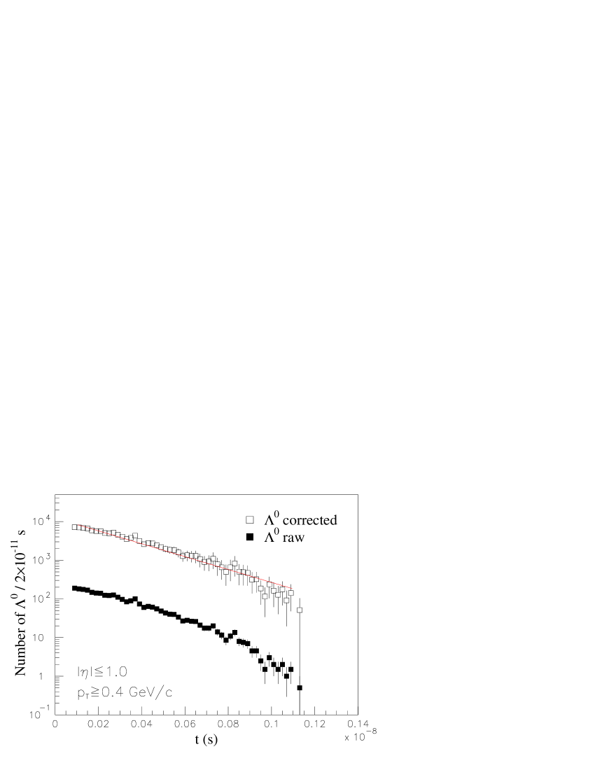
Figure 3: Raw and corrected ${\it K}^{0}_{s}$ and $\Lambda^{0}$ proper lifetime distributions for 1800 GeV data. The line represents the best exponential fit to the data.

In order to check the selection requirements and the quality of the efficiency correction, the raw and corrected proper lifetime distributions at 1800 GeV are shown in Fig. 3. Fitting to an exponential form gives a ${\it K}^{0}_{s}$ mean proper lifetime of (0.89 $\pm 0.01)\times 10^{-10}$ s ($\chi^{2}/N_{d.o.f.}$=49.7/59) for 1800 GeV and (0.90 $\pm 0.01)\times 10^{-10}$ s ($\chi^{2}/N_{d.o.f.}$=60.6/56) for 630 GeV. Both values are consistent with the world average values pdg . The same fit to the $\Lambda^{0}$ proper lifetime distributions gives a mean of (2.61 $\pm 0.07)\times 10^{-10}$ s ($\chi^{2}/N_{d.o.f.}$=44.2/49) for 1800 GeV and (2.61 $\pm 0.07)\times 10^{-10}$ s ($\chi^{2}/N_{d.o.f.}$=57.4/50) for 630 GeV. The proper lifetime regions used for the fit are $\tau>0.7\times 10^{-10}$ s (${\it K}^{0}_{s}$) and $\tau>10^{-10}$ s ($\Lambda^{0}$).

The number of undetected $V^{0}$ extracted from the fitted $p_{T}$ curve is also checked. The proper lifetime distributions of Fig. 3 are fitted to an exponential form with fixed slope (the ${\it K}^{0}_{s}$/$\Lambda^{0}$ mean lifetimes pdg , $\tau_{K^{0}_{s}}=0.8935\times 10^{-10}$ s; $\tau_{\Lambda^{0}}=2.632\times 10^{-10}$ s) in the region $\tau>0.7\times 10^{-10}$ s ($\tau>10^{-10}$ s for $\Lambda^{0}$) and the fitted curves are integrated down to $\tau=0$. The number of undetected ${\it K}^{0}_{s}(\Lambda^{0})$ obtained matches to 15% (30%) with the number from the $p_{T}$ distribution. Furthermore the $p_{T}$ distributions of ${\it K}^{0}_{s}(\Lambda^{0})$ with proper lifetimes greater than $0.8\times 10^{-10}s$ ($1.0\times 10^{-10}s$ for $\Lambda^{0}$) are compared with the corresponding distributions for all lifetimes; the comparison gives the same values of average $p_{T}$. When normalized to one another, the curves give a comparable number of ${\it K}^{0}_{s}(\Lambda^{0})$ in the extrapolated region.

An additional cross-check for correcting the average $p_{T}$ of the $V^{0}$ observed in events of fixed multiplicity consists of plotting the proper lifetime distribution in slices of $p_{T}$ so that each distribution corresponds to one bin in $p_{T}$. This is done for each bin in multiplicity. After fitting the distribution in the long lifetime region in each $p_{T}$ bin, the correct number of ${\it K}^{0}_{s}$ in the short lifetime region can be extrapolated from the fits. The $\langle p_{T}(V^{0})\rangle$ can then be recomputed from the modified $p_{T}$ distribution. The $p_{T}$ values obtained using the two different correction methods are consistent. In the case of $\Lambda^{0}$, no events are found with $p_{T}$ below 1 GeV/c due to the tight fiducial requirements imposed in the analysis. Therefore, in the $\Lambda^{0}$ case, the correction method based on extrapolating the proper lifetime distribution at each $p_{T}$ bin cannot be used. Because of this, the cross-checks are limited to comparing the number of extrapolated $\Lambda^{0}$ in the $p_{T}$ and proper lifetime distributions of the full data sample.

Finally, we refer to noi for a detailed discussion of the charged track selection and reconstruction efficiencies.

VI SYSTEMATIC UNCERTAINTIES

The two dominant systematic uncertainties come from the acceptance and efficiency correction procedures. As described in Section V, acceptance and efficiency corrections have been computed using MC simulation, with an additional correction applied to compensate for MC deficiencies in the low $p_{T}$ region between 0.4-0.8 GeV/c. The two correction procedures are largely independent, which allows us to evaluate the systematic uncertainties from these two sources separately. The details are described below.

1. We study the sensitivity of this measurement to the differences between the MC predictions and the shapes of the observed $V^{0}$ kinematical distributions. We use the following two sets of MC events. The first is created using the default pythia MC. The second is the one used for efficiency studies using the embedding procedure: the $V^{0}$’s in this set have non-physical distributions roughly uniform in $p_{T}$ but not in $\eta$. The different correction factors evaluated from the above data sets are applied to the measured distributions. Half the difference between the corrected distributions is taken as the systematic uncertainty on the distributions themselves, which amounts to about 10% for the ${\it K}^{0}_{s}$ and $\Lambda^{0}$ $p_{T}$ distributions, roughly constant over the whole spectrum.

The effect on the mean $p_{T}$ value is 3% for ${\it K}^{0}_{s}$ and 4% for $\Lambda^{0}$. For the ${\it K}^{0}_{s}$ and $\Lambda^{0}$ multiplicity distributions, the systematic variation ranges from 10% to $\sim$25%. As a function of $N_{ch}^{\star}$, the systematic uncertainty on the number of ${\it K}^{0}_{s}$ ranges from a few percent to roughly 20% at the highest charged multiplicities.

2. The systematic uncertainty due to the correction for the undetected $V^{0}$ in the $p_{T}$ region between 0.4 and 0.8 GeV/c has been evaluated in the following way. The procedure defined in Section V, point 7, is repeated using $p_{T}$ and proper lifetime distributions both corrected with pythia MC and with the embedding-based correction. The total number of $V^{0}$ is computed by integrating the corrected $p_{T}$ and lifetime spectra for each of the two cases. We end up with four different evaluations of the number of undetected $V^{0}$. By comparing the numbers obtained from all combinations, we observe that the largest difference amounts to about 50% of the correction value. This number is taken as the systematic uncertainty on this correction and is counted as a contribution to the systematics on the the total number of measured ${\it K}^{0}_{s}(\Lambda^{0})$.

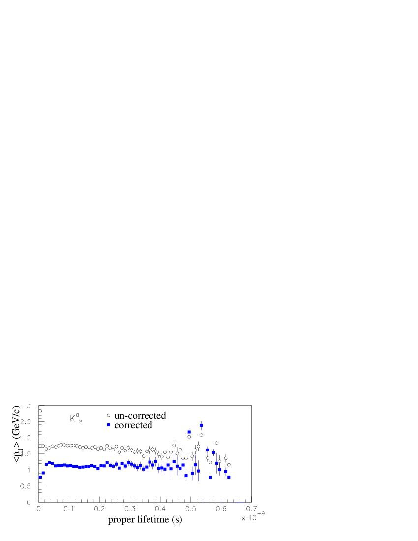
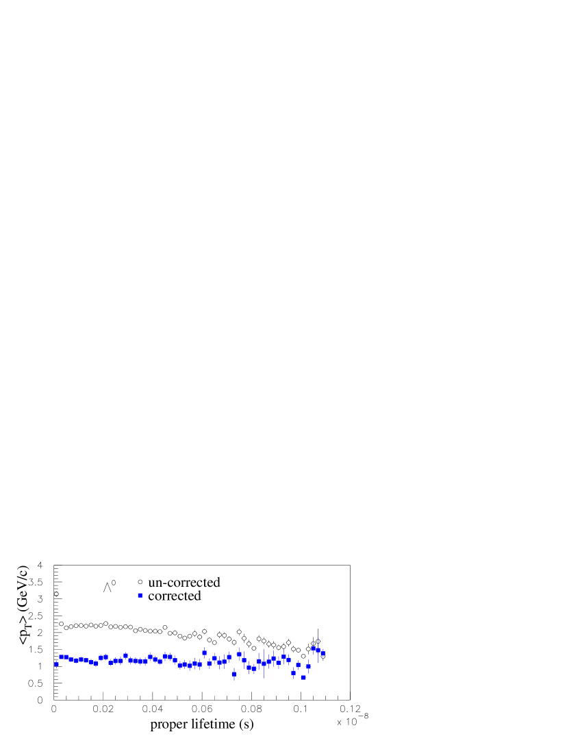
Figure 4: The mean $p_{T}$ of ${\it K}^{0}_{s}$ and $\Lambda^{0}$ as a function of proper lifetime ($t$) at 1800 GeV. Raw and corrected data are shown.

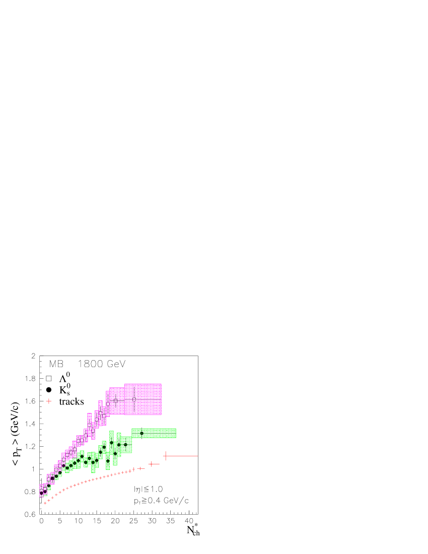
Figure 11: Average transverse momentum $\langle p_{T}\rangle$ of ${\it K}^{0}_{s}$ and $\Lambda^{0}$ at 1800 GeV as a function of the event charged multiplicity ($N_{ch}^{\star}$). MB data are shown. For comparison, the mean $p_{T}$ of charged particles measured in the same phase space region is also plotted noi . The filled squares around the points delimit the systematic uncertainties.

The mean $p_{T}$ values at fixed multiplicities are also affected by the correction for the undetected ${\it K}^{0}_{s}(\Lambda^{0})$ in the low $p_{T}$ region. The systematic uncertainty on the correction is estimated as follows. First it has been verified that the mean $p_{T}$ after correction is independent of the ${\it K}^{0}_{s}(\Lambda^{0})$ proper lifetime in the region used in this analysis (see Fig. 4). Then, starting with $p_{T}$ distributions at fixed charged multiplicity for the subset of events with ${\it K}^{0}_{s}(\Lambda^{0})$ proper lifetime greater than $0.8\times 10^{-10}s$ ($1.0\times 10^{-10}s$), the mean $p_{T}$ is computed the same way as described in Section V and the difference between the mean $p_{T}$ values for the full dataset and the high $\tau$ subset is assigned as a systematic uncertainty for this correction. Since the correction is applied only to calculations of the mean $p_{T}$ at fixed multiplicity and of the number of ${\it K}^{0}_{s}(\Lambda^{0})$, the systematic uncertainty associated with it affects only these measurements. It amounts to about 6% (10%) for the total number of ${\it K}^{0}_{s}$ ($\Lambda^{0}$) and affects the average number of ${\it K}^{0}_{s}(\Lambda^{0})$ as a function of the charged multiplicity by the same amount. These systematic uncertainties combined in quadrature with the other systematic uncertainties discussed in this section are included in Figures 11 to 16.

3. To investigate the systematic effect of the track reconstruction procedure on the efficiency correction, we compare our result with a set of MC events where the tracks are reconstructed using the CTC information alone, as opposed to the default SVX+CTC track reconstruction. We find that the variation on the final corrected $p_{T}$ distribution is negligible.

4. Other sources of systematic uncertainties include the dependence of the results on the instantaneous luminosity and the uncertainty associated with the identification and selection of good isolated $p\bar{p}$  interactions from secondary or closely spaced event vertices (see noi ). The first may affect the results because higher luminosity gives higher detector occupancy which in turn can alter the $V^{0}$ identification. This has been investigated by analyzing data samples recorded at different instantaneous luminosities. The results show no observable effect. The second source can lead to incorrect event selection and produce associations of tracks that fake a $V^{0}$. This source has been investigated by comparing data samples with different requirements for a good $p\bar{p}$ vertex noi . The results give systematic variations smaller than 9% on the overall number of ${\it K}^{0}_{s}(\Lambda^{0})$.

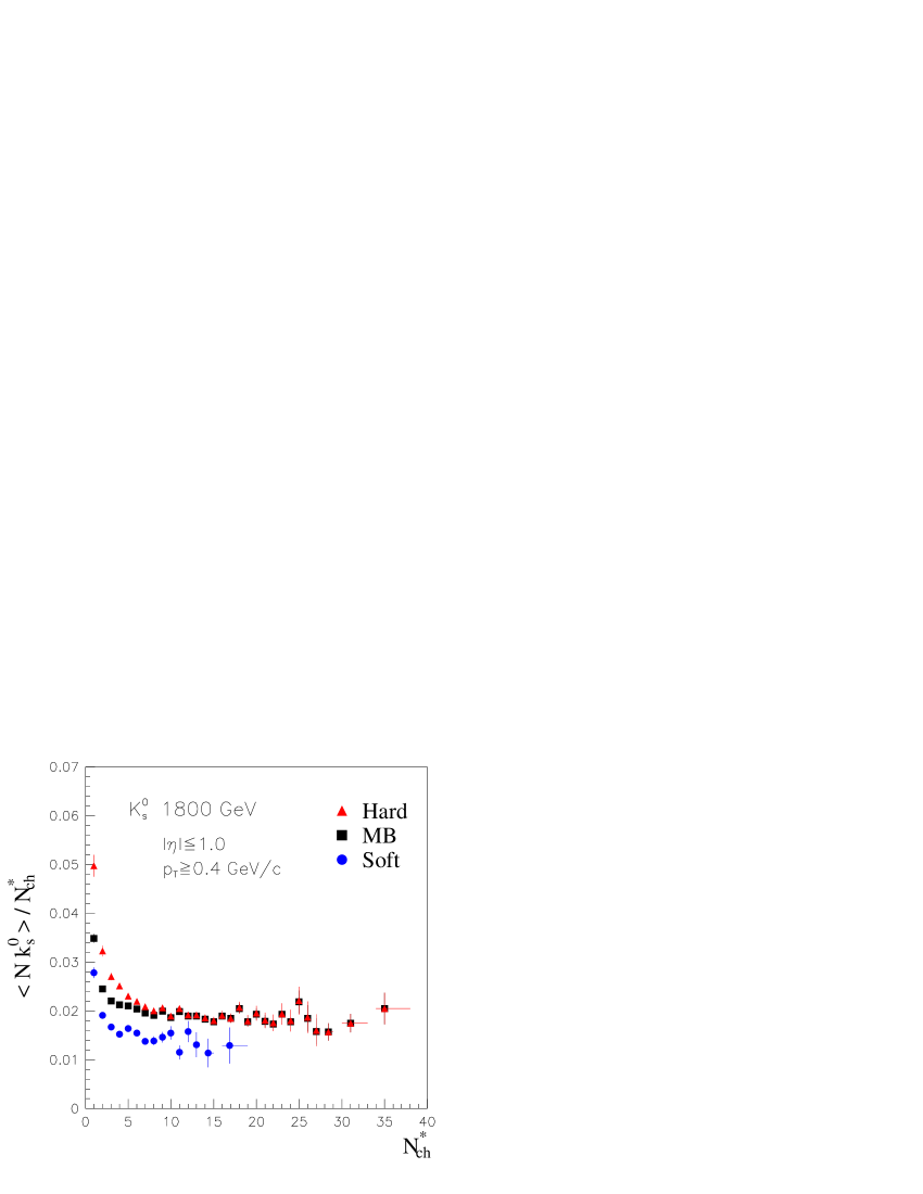
Figure 17: Mean number of ${\it K}^{0}_{s}$ per event divided by the charged multiplicity ($N_{ch}^{\star}$) and plotted as a function of $N_{ch}^{\star}$. The MB, $soft$ and $hard$ data at 1800 GeV are shown.

5. The uncertainty on the correction is distributed in different ways for different observables. As a consequence, the integral of the corrected distribution of each variable is different. For example, the total number of ${\it K}^{0}_{s}(\Lambda^{0})$ extracted from the integral of the corrected $p_{T}$ distribution may be very different from that extracted from the multiplicity distribution. In particular, as discussed in the previous section, the $p_{T}$ correction has been observed to be unreliable for $p_{T}$ $\sim$$<$ 0.7 GeV/c where a large part of the $V^{0}$ cross-section lies, so that the area under the distribution may be subject to large uncertainties. Given this, we use the global (integrated) correction from the pythia MC as a correction factor for the total number of ${\it K}^{0}_{s}(\Lambda^{0})$. We renormalize each distribution to this number to which we attribute a 30% systematic uncertainty. This value is determined as the maximum difference that was found between the global corrected number of $V^{0}$ and the integral of any corrected distribution. Such uncertainty reflects on the ${\it K}^{0}_{s}$/$\pi$ ratios and on the absolute scale of the ratios of the mean number of ${\it K}^{0}_{s}(\Lambda^{0})$ to the charged multiplicity plotted in Figures 17 to 20.

Table 3 reports a summary of all the systematic uncertainties discussed.

VII ANALYSIS RESULTS

VII.1 Results

All data presented are subject to $p_{T}$ $\geq$ 0.4 GeV/c and $|\eta|\leq$ 1 requirements, as specified in Section III, and are corrected for acceptance and vertex-finding efficiency. Systematic uncertainties are not included except where explicitly stated. Table 1 shows the raw and corrected numbers of ${\it K}^{0}_{s}(\Lambda^{0})$ selected in our fiducial region for the full MB sample as well as for the soft and the hard samples. The corrected mean number of ${\it K}^{0}_{s}(\Lambda^{0})$ per event in each sample is also shown; systematic uncertainties are included.

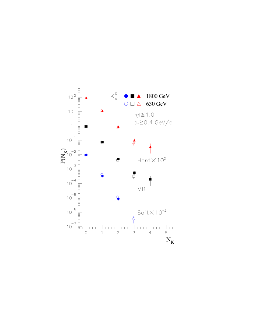
Figure 5: Distribution of the multiplicity of ${\it K}^{0}_{s}$ at 1800 (full symbols) and 630 GeV (open symbols). P($N_{K}$) = (number of events with $N_{K}$ ${\it K}^{0}_{s}$)/(total number of events). MB, $soft$ (divided by 100) and $hard$ data (multiplied by 100) are shown.

In Fig. 5 for the ${\it K}^{0}_{s}$ and in Fig. 6 for the $\Lambda^{0}$, the normalized multiplicity of ${\it K}^{0}_{s}(\Lambda^{0})$ for the MB, soft and hard events is shown separately for the $\sqrt{s}$=1800 GeV (solid symbols) and 630 GeV (open symbols) data. The probability of producing one or more $\Lambda^{0}$ is lower than the equivalent ${\it K}^{0}_{s}$ probability, and the difference increases with $V^{0}$ multiplicity. This behavior is more pronounced in the $soft$ subsample. The results shown in Figures 5 and 6, with their statistical errors, are reported in Table 4.

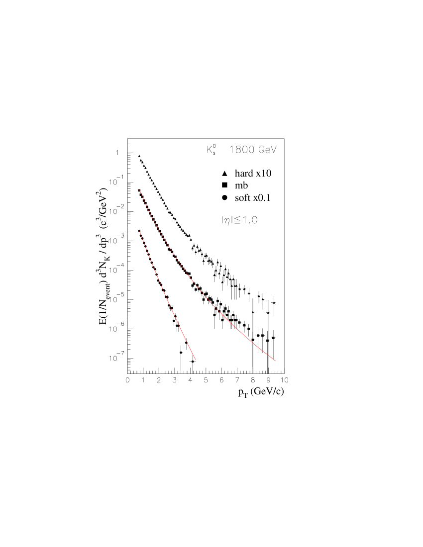
Figure 7: ${\it K}^{0}_{s}$ inclusive invariant $p_{T}$ distributions at 1800 GeV. MB, $soft$ and $hard$ data are shown, normalized to the number of events in each sample. E is the particle energy and $N_{event}$ is the total number of events which contribute to the distribution. To separate the curves, $hard$ data points are multiplied by 10 and $soft$ data points by 0.1. The solid lines represent the best fits to Eq.(2) of the text.

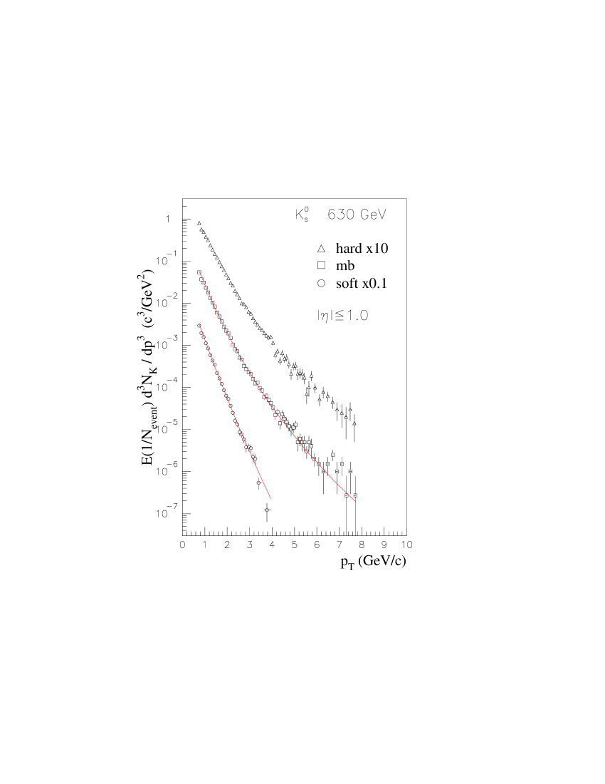
Figure 8: ${\it K}^{0}_{s}$ inclusive invariant $p_{T}$ distributions at 630 GeV MB, $soft$ and $hard$ data are shown, normalized to the number of events in each sample. E is the particle energy and $N_{event}$ is the total number of events which contribute to the distribution. To separate the curves, $hard$ data points are multiplied by 10 and $soft$ data points by 0.1. The solid lines represent the best fits to Eq.(2) of the text.

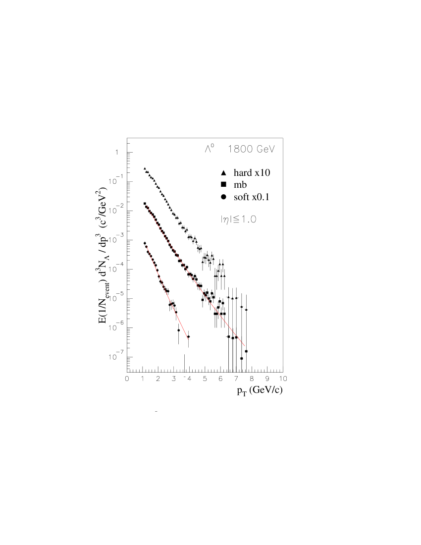
Figure 9: $\Lambda^{0}$ inclusive invariant $p_{T}$ distributions at 1800 GeV. MB, $soft$ and $hard$ data are shown, normalized to the number of events in each sample. E is the particle energy and $N_{event}$ is the total number of events which contribute to the distribution. To separate the curves, $hard$ data points are multiplied by 10 and $soft$ data points by 0.1. The solid lines represent the best fits to Eq.(2) of the text.

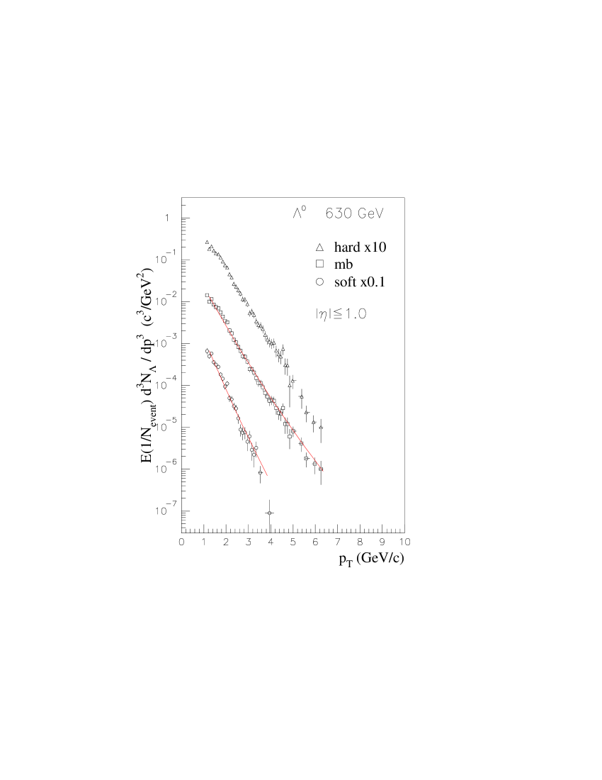
Figure 10: $\Lambda^{0}$ inclusive invariant $p_{T}$ distributions at 630 GeV. MB, $soft$ and $hard$ data are shown, normalized to the number of events in each sample. E is the particle energy and $N_{event}$ is the total number of events which contribute to the distribution. To separate the curves, $hard$ data points are multiplied by 10 and $soft$ data points by 0.1. The solid lines represent the best fits to Eq.(2) of the text.

The invariant $p_{T}$ inclusive distributions of ${\it K}^{0}_{s}$ are shown in Figures  7 and 8 at the two energies for the full MB, $soft$ and $hard$ samples. Data are normalized to the number of events in each sample. Figures 9 and 10 show the same $p_{T}$ distributions for the $\Lambda^{0}$.

The dependence of the ${\it K}^{0}_{s}$ and $\Lambda^{0}$ average $p_{T}$, calculated as described in Eq. (3), on the event charged multiplicity is shown in Figures 11 - 13 (1800 GeV) and  14 - 16 (630 GeV). The mean $p_{T}$ of primary charged tracks measured in the same phase space region, as published in noi , is also shown for comparison. For the ${\it K}^{0}_{s}$ dataset, in the region ranging from 0.4 to 0.8 GeV/c, the corrected data points are assumed to lay on a curve of form (2) extrapolated from the fit to the measured data points in the region $p_{T}>$0.8 GeV/c  (details of the correction procedure are described in Section V). Note, that with the kinematical selection used in this analysis, no events with $p_{T}$($\Lambda^{0}$)$<$1 GeV/c were observed. For the measurement of $\langle p_{T}\rangle$, we fit the spectrum in the region of $p_{T}$$>$1.1 GeV/c using Eq.(2) and extrapolate down to $p_{T}$=0.4 GeV/c. We define the $\langle p_{T}\rangle$ as the mean value of the fitted function. This definition is adopted in order to compare the $\langle p_{T}\rangle$ with that of ${\it K}^{0}_{s}$ and of charged tracks.

Figures 17 to 20 show the ratio of the mean number of ${\it K}^{0}_{s}(\Lambda^{0})$ per event to the multiplicity as a function of the multiplicity itself. The charged particle multiplicity $N_{ch}^{\star}$ was chosen as the reference variable to analyze $V^{0}$ production. The reason for this choice is based on the observation that the event charged multiplicity is a global event variable characterizing the whole multiparticle final state and is related to the hardness of the interaction (see noi , vanH , hwa ). As in the case of charged particles, possible new structures in the $V^{0}$ final state correlations would be exhibited as a function of $N_{ch}^{\star}$. The dependence of the average $p_{T}$ on multiplicity, for example, remains unexplained in any of the current models.

VII.2 Dependence on $E_{T}$ threshold

It has been remarked in the previous sections that the identification of $soft$ and $hard$ events is essentially a matter of definition. In order to investigate the sensitivity of the above results to the the cluster energy threshold used to separate $soft$ and $hard$ events, the analysis has been repeated changing the $E_{T}$ threshold from 1.1 to 3.0 GeV. Although, as expected, the higher threshold value influences the global statistics of the $soft$ and $hard$ components, it preserves the shapes of the inclusive $p_{T}$ distributions and the characteristics of the $hard$ and the $soft$ samples, and it does not change the shape of the correlations. With the new $E_{T}$ threshold the fraction of ${\it K}^{0}_{s}$ per event rises by the same amount, around 30%, in the two samples. This means that the ratio of the rate of ${\it K}^{0}_{s}$ in $soft$ events to the same rate in $hard$ events is not influenced by the higher threshold.

VII.3 Analysis Discussion

Some simple observations can be made about Table 1. The fraction of the total ${\it K}^{0}_{s}$ that falls into the $soft$ subsample is rather small, ranging from about 30% at 630 GeV to about 18% at 1800 GeV (19% and 10% for $\Lambda^{0}$ respectively). The corrected mean number of ${\it K}^{0}_{s}$ produced per event in the full MB sample is about (8.6$\pm$2.6)% at 630 GeV and (8.8$\pm$2.6)% at 1800 GeV (respectively (3.7$\pm$1.1)% and (4.3$\pm$1.0)% for $\Lambda^{0}$).

The ${\it K}^{0}_{s}$/$\pi$ cross-section ratio may be obtained by fitting the ${\it K}^{0}_{s}$ and charged-track invariant $p_{T}$ distributions in the available $p_{T}$ range and extrapolating the fitted functions down to the minimum $p_{T}$ value. This ratio is evaluated both for $p_{T}$_min=0 GeV/c and $p_{T}$_min=0.4 GeV/c. With the above technique, a ratio of 0.13$\pm$0.04 (including the systematic uncertainty) at $\sqrt{s}$=1800 GeV and 0.18$\pm$0.05 at 630 GeV is obtained for $p_{T}$_min=0.4 GeV/c. The same ratio for $p_{T}$_min=0 GeV/c, gives 0.14$\pm$0.05 at $\sqrt{s}$=1800 GeV and 0.19$\pm$0.06 at 630 GeV (Table 2). These last measurements are compatible with the previous CDF results CDFO , though are slightly higher at $\sqrt{s}=630$ GeV. In Table 2, the corresponding values for the $soft$ and $hard$ subsamples are reported. It is remarkable that ${\it K}^{0}_{s}$/$\pi$ ratio is about two times larger in $soft$ than in MB events.

Studies of the production of strange particles ${\it K}^{0}_{s}$ and $\Lambda^{0}$ in proton-antiproton interactions at different $\sqrt{s}$ are described in Ref. UA51 at $\sqrt{s}$=540 GeV and  UA52 at 200 and 900 GeV. In Refs. CDFO , E735 , alex , results at $\sqrt{s}$=1800 GeV are presented. Comparison with our results is restricted to the full MB samples; furthermore, it should be noted that here no absolute cross-sections are provided. Comparison with Refs. UA51 -E735 also requires taking into account the different $p_{T}$ and $\eta$ regions selected.

A direct comparison of the invariant $p_{T}$ distribution of ${\it K}^{0}_{s}$ can be done with Ref. CDFO . There the $p_{T}$ distribution of ${\it K}^{0}_{s}$ is fitted to the functional power-law form of Eq.(2), fixing the parameter $p^{0}$ to 1.3 GeV/c. The average $\overline{p_{T}}$ is computed from the parameters of the fit as:

$$\overline{p_{T}}=2\frac{p^{0}}{n-3}$$ (4)

With the new increased statistics and larger $p_{T}$ range, the fit with the $p^{0}$ parameter fixed, while giving a reasonable description of the $p_{T}$ spectrum in the low-$p_{T}$ region, does not describe the data at higher $p_{T}$. It yields a $\overline{p_{T}}$ compatible with the previous one (see Table 5) but with a large $\chi^{2}/N_{d.o.f.}$. The best fit to our distribution (shown in Figures 7 to 10 for the $soft$ and MB samples) is obtained with this form when all three parameters are allowed to vary freely and the fit region is restricted to $p_{T}$ $>$1 GeV/c. A summary of the results is reported in Table 5. The measurements reported in Refs. UA51 -alex were done at different energies and in different phase space regions.

From our best fit of MB sample data at 1800 GeV (630 GeV), the mean $p_{T}$ of ${\it K}^{0}_{s}$ is (0.75 $\pm$ 0.07) GeV/c ((0.70 $\pm$ 0.08) GeV/c). These values are significantly higher than the previous CDF measurements due to the higher statistics in the high $p_{T}$ tail of the distribution.

Taking into account the different conditions and the method of measurement, it is possible to compare to UA5 data (Refs. UA51 , UA52 ) as well; our present measurement is also higher in this case. For completeness, the fit results of the $p_{T}$ invariant distribution for the $soft$ subsample are also reported in Table 5. A second fitting function used is of the form:

$$E\frac{d^{3}N_{\it k}}{dp^{3}}=exp(A+B\mbox{$p_{T}$}),\ \ \ \mathrm{where}\ \ \ \overline{p_{T}}=-{\frac{2}{B}}\cdot$$ (5)

At both energies, we obtain a good $\chi^{2}/N_{d.o.f.}$ using this function (see Table 5). Therefore, the shape of the $soft$ distribution is also well described by an exponential function; the mean $p_{T}$ of the fit is generally larger than what is obtained using Eq.(2). For $\Lambda^{0}$, a systematically higher mean $p_{T}$ than other experiments at equivalent energy is obtained (compare with Refs. UA52 and E735 ). In this case as well, MB data can be equally well fitted by form (2) and by an exponential function. A summary of these results is in Table 6.

The increase of the mean $p_{T}$ (computed as in Eq. (3)) of the observed ${\it K}^{0}_{s}$ as a function of the event charged multiplicity is always larger than that of charged tracks. The increase for $\Lambda^{0}$ is even larger, leading to the conclusion that it depends on the particle mass, as expected. A similar analysis is also reported in Ref. alex . A direct comparison is not possible because of the different $p_{T}$ range and $\eta$ acceptance, which reflect in larger multiplicities. However, a rise in mean $p_{T}$ with heavier particle masses is clearly observed.

In the analysis of charged tracks noi , all the correlations examined in the MB and in the $hard$ samples showed different behaviors with respect to $E_{cms}$, while a clear invariance was seen in the $soft$ sample. With the available ${\it K}^{0}_{s}(\Lambda^{0})$ statistics it is not possible to discern any difference in the $\langle p_{T}\rangle$ dependence on multiplicity at the two energies, even in the full MB sample. Nevertheless, the behavior of the three subsamples is clearly different. We note that the mean ${\it K}^{0}_{s}(\Lambda^{0})$ $p_{T}$ increases with $N_{ch}^{\star}$ also in the $soft$ subsample, a feature that is not explained by the current models(sjo ,noi ,vanH ,hwa ,barsh ). This observation also holds for charged hadrons, as discussed in noi .

The ratios of the mean numbers of ${\it K}^{0}_{s}(\Lambda^{0})$ per event to the charged multiplicity drop in the first few bins (0 $\sim$$<$ $N_{ch}^{\star}$ $\sim$$<$ 6) and are roughly constant for $N_{ch}^{\star}$ $\geq$ 6 (MB sample) for both ${\it K}^{0}_{s}$ and $\Lambda^{0}$. The dependence on $N_{ch}^{\star}$ is more pronounced for ${\it K}^{0}_{s}$ than for $\Lambda^{0}$. The fraction of $\Lambda^{0}$ per event and per track is obviously smaller than that of ${\it K}^{0}_{s}$ and for both is larger at 630 GeV than at 1800 GeV. Finally, the dependencies of the number of $\Lambda^{0}$ for the $soft$ and the MB samples on $N_{ch}^{\star}$, besides differing by about a factor of two, are both roughly flat and different in shape from the corresponding of the ${\it K}^{0}_{s}$ distributions.

VIII CONCLUSIONS

The present measurements extend the studies of charged particle properties in MB $p\bar{p}$ interactions to ${\it K}^{0}_{s}$ and $\Lambda^{0}$ production. Using the data available at the two c.m.s. energies obtained under the same experimental conditions and similar statistics, we are able to directly compare the $V^{0}$ production properties at the two c.m.s. energies. Our results offer new findings and significant improvements to the existing knowledge of $V^{0}$ production. We summarize our results as follows:

• The overall production rates of ${\it K}^{0}_{s}$ and $\Lambda^{0}$ are in agreement with previous measurements.

• The inclusive $p_{T}$ spectra of ${\it K}^{0}_{s}$ and $\Lambda^{0}$ now extend to $p_{T}$ $\geq$ 8 GeV/c. The ${\it K}^{0}_{s}$ distribution shows a more detailed shape in the high $p_{T}$ region when compared to previous data. For both ${\it K}^{0}_{s}$ and $\Lambda^{0}$, we measure an average $p_{T}$ significantly higher than previous results.

• New results are presented on the distribution of ${\it K}^{0}_{s}$ and $\Lambda^{0}$ multiplicity.

• For the first time, the MB sample has been used to analyze $V^{0}$ production properties in its $soft$ and $hard$ components. Inclusive $p_{T}$ and multiplicity distributions of $V^{0}$ are shown for the $soft$ and $hard$ data.

• Analyses of the dependence of the mean ${\it K}^{0}_{s}(\Lambda^{0})$ $p_{T}$ with the event charged multiplicity are presented. The observed dependence is not explained by the current theoretical models. Comparison with an analogous study performed on charged tracks indicates that the rate of the dependence grows with particle mass. An increase of the mean $p_{T}$ is observable also in the $soft$ subsample alone.

• The event charged multiplicity has been adopted as the independent variable to analyze the ratio of the mean number of ${\it K}^{0}_{s}(\Lambda^{0})$ per event to the number of primary charged particles. For both ${\it K}^{0}_{s}$ and $\Lambda^{0}$ this ratio rises toward very low multiplicity, remaining roughly constant for $N_{ch}^{\star}$ $\sim$$>$ 5.

Table 1: Raw and corrected numbers of ${\it K}^{0}_{s}$ and $\Lambda^{0}$ found in each data set. In the rightmost three columns the fraction of ${\it K}^{0}_{s}(\Lambda^{0})$ per event is shown. The uncertainties on all the corrected numbers and fraction of ${\it K}^{0}_{s}(\Lambda^{0})$ per event include the systematic uncertainty. The total number of MB events at $\sqrt{s}$=1800 GeV (630 GeV) is 2,079,558(1,963,157).

		RAW			CORRECTED			FRACTION of ${\it K}^{0}_{s}(\Lambda^{0})$/EVENT (%)
		MB	Soft	Hard	MB ($\times 10^{3}$)	Soft ($\times 10^{3}$)	Hard ($\times 10^{3}$)	MB	Soft	Hard
1800	${\it K}^{0}_{s}$	36642	6733	29909	180$\pm$50	34$\pm$10	150$\pm$40	8.8$\pm$2.6	3.5$\pm$1.0	13.3$\pm$4.0
GeV	$\Lambda^{0}$	7518	782	6736	90$\pm$30	9$\pm$3	80$\pm$20	4.3$\pm$1.0	1.0$\pm$0.3	7.2$\pm$2.2
630	${\it K}^{0}_{s}$	32222	9835	22387	170$\pm$50	50$\pm$15	120$\pm$35	8.6$\pm$2.6	4.5$\pm$1.4	14.3$\pm$4.3
GeV	$\Lambda^{0}$	5883	1098	4785	70$\pm$20	13$\pm$4	60$\pm$20	3.7$\pm$1.1	1.2$\pm$0.4	7.1$\pm$2.1

Table 2: ${\it K}^{0}_{s}$/$\pi$ ratio in each data set. Data computed in the full $p_{T}$ range and for $p_{T}$$\geq$ 0.4 GeV/c are shown. The ratios are evaluated integrating the $p_{T}$ distributions by extrapolating the fitted function down to $p_{T}$_min=0. (0.4) GeV/c. Here efficiency corrections and systematic uncertainties are included.

	$p_{T}$min (GeV/c)	MB	Soft	Hard
1800	0.0	0.14$\pm$0.05	0.38$\pm$0.12	0.11$\pm$0.04
	0.4	0.13 $\pm$ 0.04	0.30 $\pm$ 0.09	0.11 $\pm$ 0.03
630	0.0	0.19$\pm$0.06	0.42$\pm$0.13	0.14$\pm$0.05
	0.4	0.18 $\pm$ 0.05	0.33 $\pm$ 0.10	0.18 $\pm$ 0.06

Table 3: Summary of all systematic uncertainties. For each systematic uncertainty source its effect on the various measured quantities is reported. The symbol “-” means no effect on the corresponding quantity.

Systematic	$\langle p_{T}\rangle$ vs Mult.	$p_{T}$ distr.	N($V^{0}$) distr.	$<$N($V^{0}$)$>$ vs Mult	N($V^{0}$)	$K/\pi$
uncertainty	(included	(————————-		not included in figures	—————)	(included
source	in figures)					in table 2)
MC simulation	3% (${\it K}^{0}_{s}$)	10%	10-25%	2-20%	—	—
	4% ($\Lambda^{0}$)
Low-$p_{T}$	3-20 %	—	5% (${\it K}^{0}_{s}$)	5% (${\it K}^{0}_{s}$)	5% (${\it K}^{0}_{s}$)	6%
extrapolation			10% ($\Lambda^{0}$)	10% ($\Lambda^{0}$)	10% ($\Lambda^{0}$)
Primary vertex	—	—	———————————- $<9\%$ ——————————
selection
Global normalization	—	—————————————— $<30\%$ ————————————
factor

Table 4: Number of events with $N_{K}$ ${\it K}^{0}_{s}$ ($N_{\Lambda}$ $\Lambda^{0}$) divided by the total number of events. MB, $soft$ and $hard$ data at 1800 and 630 GeV are reported.

	$N_{K/\Lambda}$	——————- 1800 GeV ——————-			——————- 630 GeV ——————-
		MB ($\times 10^{-3}$)	Soft ($\times 10^{-3}$)	Hard ($\times 10^{-3}$)	MB ($\times 10^{-3}$)	Soft ($\times 10^{-3}$)	Hard ($\times 10^{-3}$)
	0	919$\pm$ 7	966$\pm$ 2	880$\pm$ 10	920$\pm$ 10	956$\pm$ 5	870$\pm$ 20
	1	80$\pm$ 10	33$\pm$ 6	110$\pm$ 20	80$\pm$ 20	40$\pm$ 10	120$\pm$ 30
${\it K}^{0}_{s}$	2	5$\pm$ 1	0.9$\pm$ 0.2	9$\pm$ 2	4$\pm$ 1	1.2$\pm$ 0.3	8$\pm$ 2
	3	0.6$\pm$ 0.2		1.0$\pm$ 0.3	0.3$\pm$ 0.1	0.04$\pm$ 0.02	0.7$\pm$ 0.3
	4	0.2$\pm$ 0.1		0.4$\pm$ 0.2
	0	958$\pm$ 5	990.3$\pm$ 0.1	930$\pm$ 10	964$\pm$ 5	988.3$\pm$ 0.1	930$\pm$ 10
$\Lambda^{0}$	1	40$\pm$ 20	10$\pm$ 4	70$\pm$ 30	40$\pm$ 20	12$\pm$ 5	70$\pm$ 30
	2	1.6$\pm$ 0.8	0.08$\pm$ 0.05	3$\pm$ 1	0.9$\pm$ 0.5		2$\pm$ 1

Table 5: Results of the fit to the invariant $p_{T}$ distribution of ${\it K}^{0}_{s}$. Data at different $E_{cms}$ are reported (for different experiments the parameters of the fit were reported when available). Parameters $p^{0}$ and $n$ refer to the power-law (P.L.) function [Eq.(2)], $B$ to the exponential (Exp.) form [Eq.(5)]. CDF-0 refers to the so called Run-0 of the Tevatron CDFO and CDF-I to Run I data (this analysis).

Experiment	Data Set	$\overline{p_{T}}$	$p^{0}$ (P.L.)	$n$ (P.L.)	B (Exp.)	$\chi^{2}/N_{d.o.f.}$
($\sqrt{s}$ in GeV)		(GeV/c)	(GeV/c)
UA5(*) (546)UA51	MB	0.58$\pm$0.04	–	–		1.15
CDF-0 (630)CDFO	MB	0.5$\pm$0.1	1.3(fixed)	7.9$\pm$0.03		3.9
CDF-I (630)	MB	0.70$\pm$0.08	3.3$\pm$0.2	12.6$\pm$0.6		68/57
UA5(*) (900)UA52	MB	0.63$\pm$0.03	–	–		0.5
CDF-0 (1800)CDFO	MB	0.60$\pm$0.03	1.3(fixed)	7.7$\pm$0.2		0.74
CDF-I (1800)	MB	0.58$\pm$0.02	1.3(fixed)	7.49$\pm$0.02		265/68
CDF-I (1800)	MB	0.75$\pm$0.07	3.29$\pm$0.08	11.7$\pm$0.1		67/67
CDF-I (630)	Soft	0.58$\pm$0.04	9.0$\pm$0.1	33.7$\pm$0.1		29/22
CDF-I (630)	Soft	0.64$\pm$0.02			-3.12$\pm$0.03	24/23
CDF-I (1800)	Soft	0.62$\pm$0.02	9.5$\pm$0.3	33.7$\pm$0.9		23/25
CDF-I (1800)	Soft	0.67$\pm$0.02			-3.00$\pm$0.04	29/26
(*) UA5 fits to a power-law form in $p_{T}>$0.4 together with an exponential form in $p_{T}<$0.4 GeV/c.

Table 6: Results of the fit to the invariant $p_{T}$ distribution of $\Lambda^{0}$. Data at different $E_{cms}$ are reported (for different experiments the parameters of the fit were reported when available). Parameters $p^{0}$ and $n$ refer to the power-law (P.L.) function [Eq.(2)], $B$ to the exponential (Exp.) form [Eq.(5)]. CDF-I refers to Run I data (this analysis).

Experiment	Data Set	$\overline{p_{T}}$	$p^{0}$ (P.L.)	$n$ (P.L.)	B (Exp.)	$\chi^{2}/N_{d.o.f.}$
($\sqrt{s}$ in GeV)		(GeV/c)	(GeV/c)
UA5 (546)UA51	MB	0.62$\pm$0.08	–	–		–
CDF-I (630)	MB	0.91$\pm$0.07	12.3$\pm$0.1	30.1$\pm$0.2		59/35
CDF-I (630)	MB	0.98$\pm$0.01			-2.05$\pm$0.03	50/36
UA5 (900)UA52	MB	0.97$\pm$0.01			–	–
CDF-I (1800)	MB	0.97$\pm$0.09	12.4$\pm$0.1	28.6 $\pm$ 0.09		41/45
CDF-I (1800)	MB	1.04$\pm$0.01			-1.92$\pm$0.02	55/46
CDF-I (630)	Soft	0.67$\pm$0.09	10.0$\pm$0.2	33.0$\pm$0.2		31/24
CDF-I (630)	Soft	0.73$\pm$0.1			-2.74$\pm$0.05	28/25
CDF-I (1800)	Soft	0.64$\pm$0.05	9.5$\pm$3.3	33.0 $\pm$0.2		29/22
CDF-I (1800)	Soft	0.73$\pm$0.10			-2.74$\pm$0.05	25/23

Figure 1: Invariant mass with a $\pi-\pi$ and $\pi$-p mass assignment for oppositely signed track pairs passing all selection requirements but allowing the mass to be within 10$\sigma$ from the nominal mass. The background includes the contamination by ${\it K}^{0}_{s}$ in the $\Lambda^{0}$ sample and vice versa. 1800 GeV data are shown.

Figure 2: Overall correction factors at 1800 GeV for ${\it K}^{0}_{s}(\Lambda^{0})$ as a function of the transverse momentum. The correction factors are defined in the text.

Figure 6: Distribution of the multiplicity of $\Lambda^{0}$ at 1800 (full symbols) and 630 GeV (open symbols). P($N_{\Lambda}$) = (number of events with $N_{\Lambda}$ $\Lambda^{0}$)/(total number of events). MB, $soft$ (divided by 100) and $hard$ data (multiplied by 100) are shown.

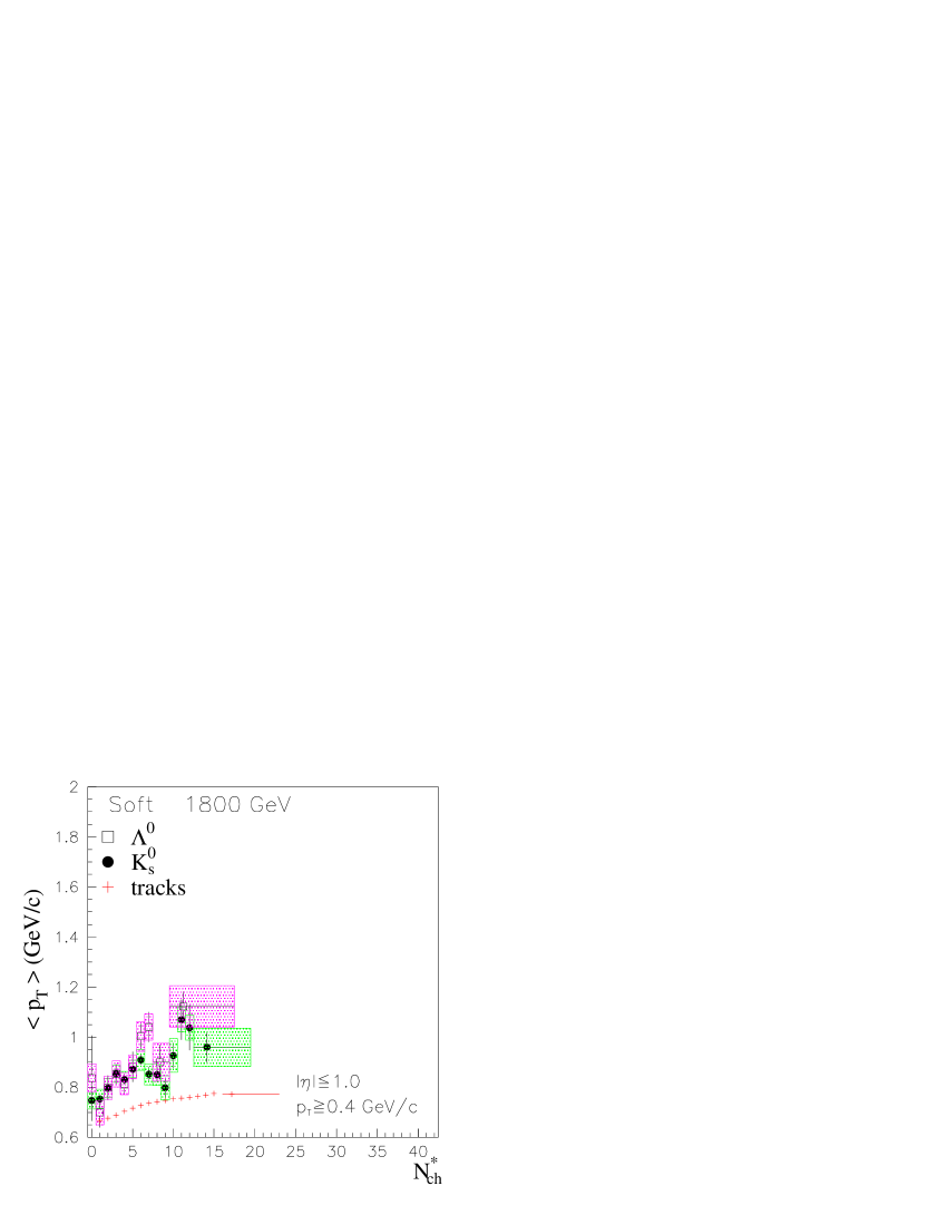
Figure 12: Average transverse momentum $\langle p_{T}\rangle$ of ${\it K}^{0}_{s}$ and $\Lambda^{0}$ at 1800 GeV as a function of the event charged multiplicity ($N_{ch}^{\star}$). $Soft$ data are shown. For comparison, the mean $p_{T}$ of charged particles measured in the same phase space region is also plotted noi . The filled squares around the points delimit the systematic uncertainties.

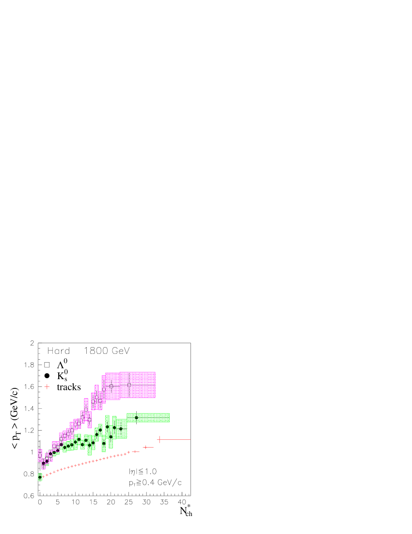
Figure 13: Average transverse momentum $\langle p_{T}\rangle$ of ${\it K}^{0}_{s}$ and $\Lambda^{0}$ at 1800 GeV as a function of the event charged multiplicity ($N_{ch}^{\star}$). $Hard$ data are shown. For comparison, the mean $p_{T}$ of charged particles measured in the same phase space region is also plotted noi . The filled squares around the points delimit the systematic uncertainties.

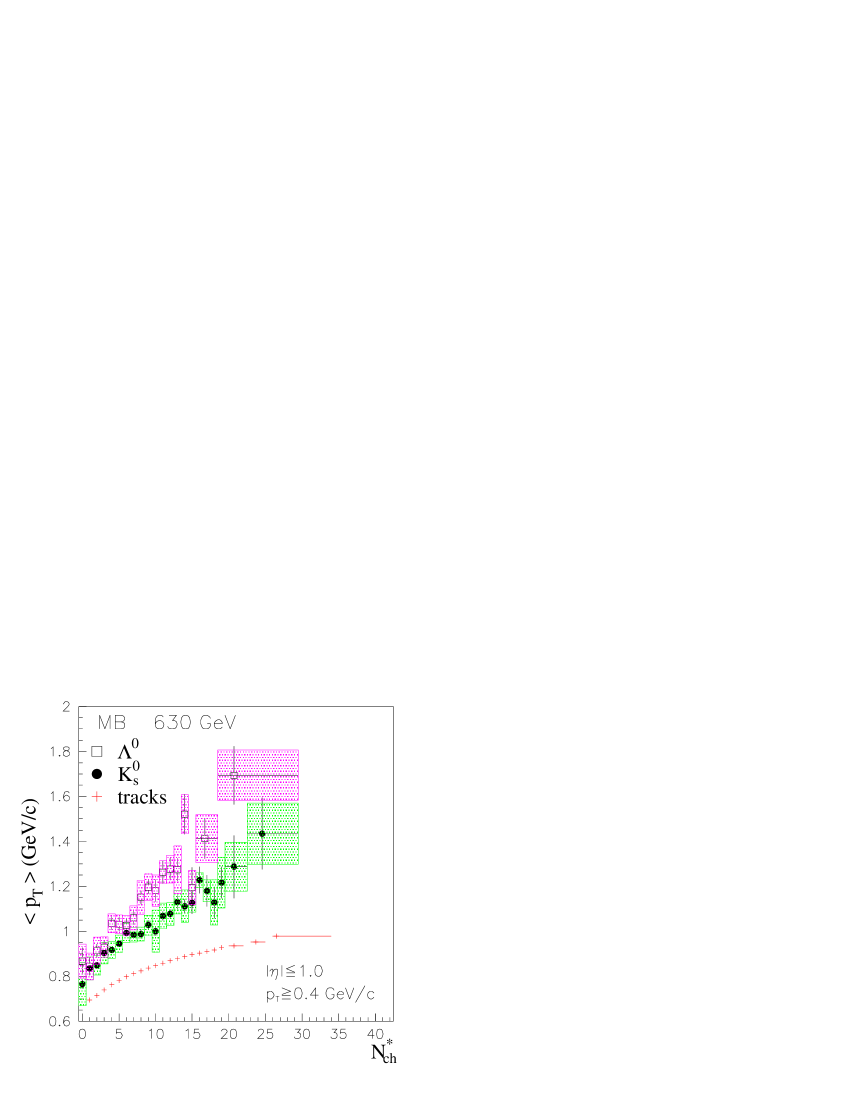
Figure 14: Average transverse momentum $\langle p_{T}\rangle$ of ${\it K}^{0}_{s}$ and $\Lambda^{0}$ at 630 GeV as a function of the event charged multiplicity ($N_{ch}^{\star}$). MB data are shown. For comparison, the mean $p_{T}$ of charged particles measured in the same phase space region is also plotted noi . The filled squares around the points delimit the systematic uncertainties.

Figure 15: Average transverse momentum $\langle p_{T}\rangle$ of ${\it K}^{0}_{s}$ and $\Lambda^{0}$ at 630 GeV as a function of the event charged multiplicity ($N_{ch}^{\star}$). $Soft$ data are shown. For comparison, the mean $p_{T}$ of charged particles measured in the same phase space region is also plotted noi . The filled squares around the points delimit the systematic uncertainties.

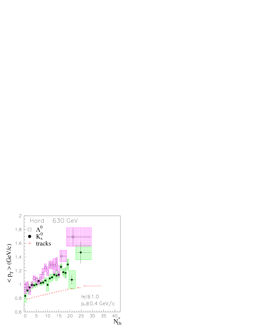
Figure 16: Average transverse momentum $\langle p_{T}\rangle$ of ${\it K}^{0}_{s}$ and $\Lambda^{0}$ at 630 GeV as a function of the event charged multiplicity ($N_{ch}^{\star}$). $Hard$ data are shown. For comparison, the mean $p_{T}$ of charged particles measured in the same phase space region is also plotted noi . The filled squares around the points delimit the systematic uncertainties.

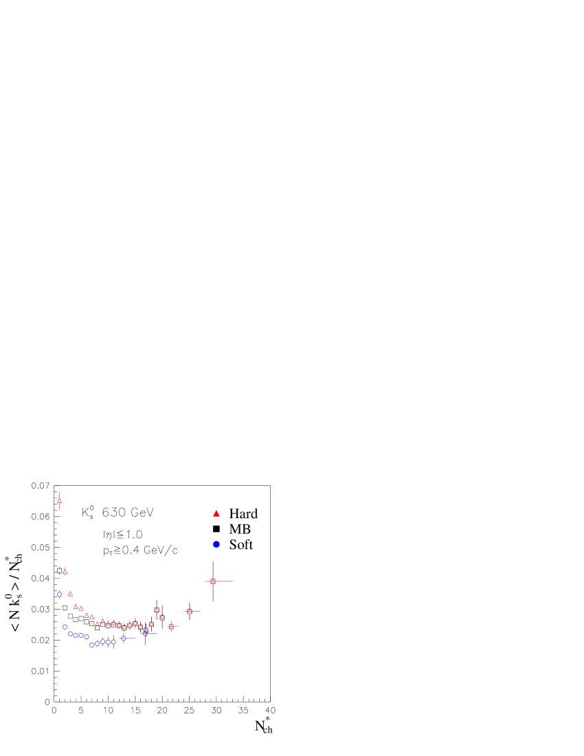
Figure 18: Mean number of ${\it K}^{0}_{s}$ per event divided by the charged multiplicity  ($N_{ch}^{\star}$) and plotted as a function of $N_{ch}^{\star}$. The MB, $soft$ and $hard$ data at 1800 GeV are shown.

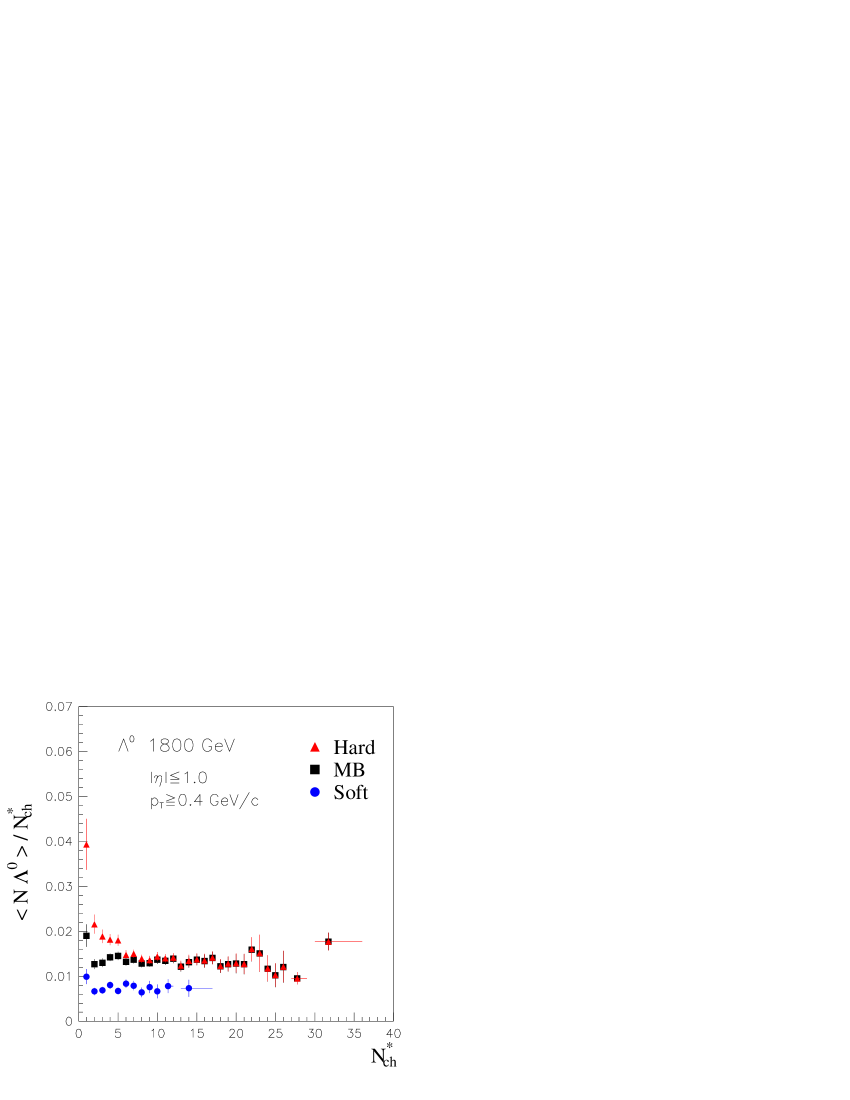
Figure 19: Mean number of $\Lambda^{0}$ per event divided by the charged multiplicity ($N_{ch}^{\star}$) and plotted as a function of $N_{ch}^{\star}$. The MB, $soft$ and $hard$ data at 1800 GeV are shown.

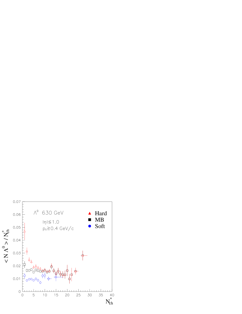
Figure 20: Mean number of $\Lambda^{0}$ per event divided by the charged multiplicity ($N_{ch}^{\star}$) and plotted as a function of $N_{ch}^{\star}$. The MB, $soft$ and $hard$ data at 630 GeV are shown.

References

- (1) R. Ansari et al., Z. Phys. C36, 175 (1987); X. Wang and R. C. Hwa, Phys. Rev. D39, 187 (1989); UA1 Collaboration, F. Ceradini, Bari Europhys. High Energy 1985:0363.
- (2) T. Sjöstrand and M. van Zijl, Phys. Rev. D36, 2019 (1987), and references therein.
- (3) A summary of the references to these models can be found in sjo .
- (4) D. Acosta et al., Phys. Rev. D65, 072005 (2002);
- (5) F. Abe et al., Nucl. Instrum. Methods A271, 387 (1988), and references therein.
- (6) F. Abe et al., Phys. Rev. D52, 4784 (1995).
- (7) F. Bedeschi et al., Nucl. Instrum. Methods A268, 50 (1988).
- (8) F. Snider et al., Nucl. Instrum. Methods A268, 75 (1988).
- (9) F. Balka et al., Nucl. Instrum. Methods A267, 272 (1988); S. R. Hahn et al., ibid. 267, 351 (1988); K. Yasuoka et al., ibid. 267, 315 (1988); R. G. Wagner et al., ibid. 267, 330 (1988); T. Devlin et al., ibid. 268, 24 (1988); S. Bertolucci et al., ibid. 267, 301 (1988); Y. Fukui et al., ibid. 267, 280 (1988); S. Cihangir et al., ibid. 267, 249 (1988); G. Brandenburg et al., ibid. 267, 257 (1988).
- (10) As we do not distinguish from , in this paper stands for both.
- (11) Particle Data Group, Phys. Rev D66, 010001-35 (2002); Phys. Rev D66, 010001-61 (2002).
-
(12)
F. Abe et al., Phys. Rev. D56, 3811 (1997);
Phys. Rev. Lett. 79, 584 (1997);
X. Wang, Phys. Rev. D46, 1900 (1992);
UA1 Collaboration, C. Albajar et al, Nucl. Phys. B309, 405 (1988). - (13) T. Sjöstrand, Computer Phys. Commun. 82, 74 (1994); G.Marchesini, B.R.Webber, G.Abbiendi, I.G.Knowles, M.H.Seymour,and L.Stanco, Computer Phys. Commun. 67,465 (1992).
- (14) G. Arnison et al., Phys. Lett. B118, 167 (1982); F. Abe et al., Phys. Rev. Lett. 61, 1819 (1988).
- (15) L. Van Hove, Phys. Lett. B118, 138 (1982); R. Hagedorn, Rev. Nuovo Cimento 6, 10 (1983); J.D. Bjorken, Phys. Rev. D27, 140 (1983).
- (16) X. Wang and C. Hwa, Phys. Rev. D39, 187 (1989); M. Jacob, CERN preprint CERN/TH. 3515 (1983); F.W. Bopp, P. Aurenche, and J. Ranft, Phys. Rev. D33, 1867 (1986).
- (17) F.Abe et al., CDF Collaboration, Phys. Rev. D40, 3791 (1989).
- (18) K.Alpgard et al., UA5 Collaboration, Phys. Lett. B115, 65 (1982); G.J.Alner et al., UA5 Collaboration, Nucl. Phys. B258,505 (1985).
- (19) R.E.Ansorge et al., UA5 Collaboration, Phys. Lett. B199, 311 (1987).
- (20) S.Banerjee et al., E735 Collaboration, Phys. Rev. Lett. 62, 12 (1989).
- (21) T.Alexopoulus, II Int.Conf. on Phys. and Astrophys. of Quark-Gluon Plasma, Calcutta, January 1993.
- (22) S. Barshay, Phys.Lett. B127, 129 (1983).