Search for $b\rightarrow u$ transitions in $B^{-}\rightarrow D^{0}K^{-}$ and $B^{-}\rightarrow D^{*0}K^{-}$

Abstract

We search for $B^{-}\rightarrow\tilde{D}^{0}K^{-}$ and $B^{-}\rightarrow\tilde{D}^{*0}K^{-}$ and charge conjugates. Here the symbol $\tilde{D}^{0}$ indicates decay of a $D^{0}$ or $\bar{D}^{0}$ into $K^{+}\pi^{-}$, while the symbol $\tilde{D}^{*0}$ indicates decay of a $D^{*0}$ or $\bar{D}^{*0}$ to $\tilde{D}^{0}\pi^{0}$ or $\tilde{D}^{0}\gamma$. These final states can be reached through the $b\rightarrow c$ transition $B^{-}\rightarrow D^{(*)0}K^{-}$ followed by the doubly Cabibbo-Kobayashi-Maskawa (CKM)-suppressed $D^{0}\rightarrow K^{+}\pi^{-}$, or the $b\rightarrow u$ transition $B^{-}\rightarrow\kern 1.99997pt\overline{\kern-1.99997ptD}{}^{(*)0}K^{-}$ followed by the CKM-favored $\kern 1.99997pt\overline{\kern-1.99997ptD}{}^{0}\rightarrow K^{+}\pi^{-}$. The interference of these two amplitudes is sensitive to the angle $\gamma$ of the unitarity triangle. Our results are based on 232 million $\mathchar 28935\relax{(4S)}\rightarrow B\kern 1.79993pt\overline{\kern-1.79993ptB}{}$ decays collected with the BABAR detector at SLAC. We find no significant evidence for these decays. We set a limit $r_{B}\equiv|A(B^{-}\rightarrow\kern 1.99997pt\overline{\kern-1.99997ptD}{}^{0}K^{-})/A(B^{-}\rightarrow D^{0}K^{-})|<0.23$ at 90% C.L. using the most conservative assumptions on the values of the CKM angle $\gamma$ and the strong phases in the $B$ and $D$ decay amplitudes. In the case of the $D^{*}$ we set a 90% C.L. limit $r^{*2}_{B}\equiv|A(B^{-}\rightarrow\kern 1.99997pt\overline{\kern-1.99997ptD}{}^{*0}K^{-})/A(B^{-}\rightarrow D^{*0}K^{-})|^{2}<(0.16)^{2}$ which is independent of assumptions on $\gamma$ and strong phases.

I INTRODUCTION

Following the discovery of $C\!P$ violation in $B$-meson decays and the measurement of the angle $\beta$ of the unitarity triangle cpv associated with the Cabibbo-Kobayashi-Maskawa (CKM) quark mixing matrix, focus has turned towards the measurements of the other angles $\alpha$ and $\gamma$. The angle $\gamma$ is ${\rm arg}(-V_{ub}^{*}V_{ud}/V_{cb}^{*}V_{cd})$, where $V_{ij}$ are CKM matrix elements. In the Wolfenstein convention wolfenstein , $\gamma={\rm arg}(V_{ub}^{*})$.

Several proposed methods for measuring $\gamma$ exploit the interference between $B^{-}\rightarrow D^{(*)0}K^{(*)-}$ and $B^{-}\rightarrow\kern 1.99997pt\overline{\kern-1.99997ptD}{}^{(*)0}K^{(*)-}$ (Fig. 1) that occurs when the $D^{(*)0}$ and the $\kern 1.99997pt\overline{\kern-1.99997ptD}{}^{(*)0}$ decay to common final states, as first suggested in Ref. dk1 .

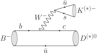
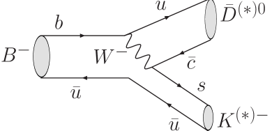
Figure 1: Feynman diagrams for $B^{-}\rightarrow D^{(*)0}K^{(*)-}$ and $\kern 1.99997pt\overline{\kern-1.99997ptD}{}^{(*)0}K^{(*)-}$. The latter is CKM and color suppressed with respect to the former. The CKM-suppression factor is $|V_{ub}V_{cs}^{*}/V_{cb}V_{us}^{*}|\approx 0.4$. The naive color-suppression factor is $\frac{1}{3}$.

As proposed in Ref. dk2 , we search for $B^{-}\rightarrow\tilde{D}^{0}K^{-}$ and $B^{-}\rightarrow\tilde{D}^{*0}K^{-},~{}\tilde{D}^{*0}\rightarrow\tilde{D}^{0}\pi^{0}$ or $\tilde{D}^{*0}\rightarrow\tilde{D}^{0}\gamma$, followed by $\tilde{D}^{0}\rightarrow K^{+}\pi^{-}$, as well as the charge conjugate (c.c.) sequences. Here the symbol $\tilde{D}^{0}$ indicates the decay of a $D^{0}$ or $\kern 1.99997pt\overline{\kern-1.99997ptD}{}^{0}$ into $K^{+}\pi^{-}$. In these processes, the favored $B$ decay ($B^{-}\rightarrow D^{(*)0}K^{-}$) followed by the doubly CKM-suppressed $D$ decay ($D^{0}\rightarrow K^{+}\pi^{-}$) interferes with the suppressed $B$ decay ($B^{-}\rightarrow\kern 1.99997pt\overline{\kern-1.99997ptD}{}^{(*)0}K^{-}$) followed by the CKM-favored $D$ decay ($\kern 1.99997pt\overline{\kern-1.99997ptD}{}^{0}\rightarrow K^{+}\pi^{-}$). The interference of the $b\rightarrow c$ ($B^{-}\rightarrow D^{(*)0}K^{-}$) and $b\rightarrow u$ ($B^{-}\rightarrow\kern 1.99997pt\overline{\kern-1.99997ptD}{}^{(*)0}K^{-}$) amplitudes is sensitive to the relative weak phase $\gamma$.

We use the notation $B^{-}\rightarrow[h_{1}^{+}h_{2}^{-}]_{D}h_{3}^{-}$ (with each $h_{i}=\pi$ or $K$) for the decay chain $B^{-}\rightarrow\tilde{D}^{0}~{}h_{3}^{-}$, $\tilde{D}^{0}~{}\rightarrow h_{1}^{+}h_{2}^{-}$. For the closely related modes with a $\tilde{D}^{*0}$, we use the same notation with the subscript $D$ replaced by $D\pi^{0}$ or $D\gamma$, depending on whether the $\tilde{D}^{*0}$ decays to $\tilde{D}^{0}\pi^{0}$ or $\tilde{D}^{0}\gamma$. We also refer to $h_{3}$ as the bachelor $\pi$ or $K$.

In the decays of interest, the sign of the bachelor kaon is opposite to that of the kaon from $\tilde{D}^{0}$ decay. It is convenient to define ratios of rates between these decays and the similar decays where the two kaons have the same sign. The decays with same-sign kaons have much higher rate and proceed almost exclusively through the CKM-favored and color-favored $B$ transition, followed by the CKM-favored $D$-decay, e.g., $B^{-}\rightarrow D^{0}K^{-}$, $D^{0}\rightarrow K^{-}\pi^{+}$. The advantage of taking ratios is that most theoretical and experimental uncertainties cancel. Thus, ignoring possible small effects due to $D$ mixing and taking into account the effective phase difference of $\pi$ between the $D^{*}$ decays in $D\gamma$ and $D\pi^{0}$ Bondar , we define the charge-specific ratios for $D$ and $D^{*}$ as:

$${\cal R}^{\pm}_{K\pi}\equiv\frac{\Gamma([K^{\mp}\pi^{\pm}]_{D}K^{\pm})}{\Gamma([K^{\pm}\pi^{\mp}]_{D}K^{\pm})}=r_{B}^{2}+r_{D}^{2}+2r_{B}r_{D}\cos(\pm\gamma+\delta),$$ (1)

$${\cal R}^{*\pm}_{K\pi,D\pi^{0}} \equiv \frac{\Gamma([K^{\mp}\pi^{\pm}]_{D\pi^{0}}K^{\pm})}{\Gamma([K^{\pm}\pi^{\mp}]_{D\pi^{0}}K^{\pm})}$$ (2)

$$= r_{B}^{*2}+r_{D}^{2}+2r_{B}^{*}r_{D}\cos(\pm\gamma+\delta^{*}),$$

and

$${\cal R}^{*\pm}_{K\pi,D\gamma} \equiv \frac{\Gamma([K^{\mp}\pi^{\pm}]_{D\gamma}K^{\pm})}{\Gamma([K^{\pm}\pi^{\mp}]_{D\gamma}K^{\pm})}$$ (3)

$$= r_{B}^{*2}+r_{D}^{2}-2r_{B}^{*}r_{D}\cos(\pm\gamma+\delta^{*}),$$

where

$$r_{B}\equiv\left|\frac{A(B^{-}\rightarrow\kern 1.99997pt\overline{\kern-1.99997ptD}{}^{0}K^{-})}{A(B^{-}\rightarrow D^{0}K^{-})}\right|,$$ (4)

$$r_{B}^{*}\equiv\left|\frac{A(B^{-}\rightarrow\kern 1.99997pt\overline{\kern-1.99997ptD}{}^{*0}K^{-})}{A(B^{-}\rightarrow D^{*0}K^{-})}\right|,$$ (5)

$$r_{D}\equiv\left|\frac{A(D^{0}\rightarrow K^{+}\pi^{-})}{A(D^{0}\rightarrow K^{-}\pi^{+})}\right|,$$ (6)

$$\delta^{(*)}\equiv\delta_{B}^{(*)}+\delta_{D},$$ (7)

and $\delta_{B}^{(*)}$ and $\delta_{D}$ are strong phase differences between the two $B$ and $D$ decay amplitudes, respectively. The value of $r_{D}$ has been measured to be $r_{D}=0.060\pm 0.002$ PDG .

We also define the charge-independent ratio

$${\cal R}_{K\pi}\equiv\frac{\Gamma([K^{+}\pi^{-}]_{D}K^{-})+\Gamma([K^{-}\pi^{+}]_{D}K^{+})}{\Gamma([K^{-}\pi^{+}]_{D}K^{-})+\Gamma([K^{+}\pi^{-}]_{D}K^{+})}$$ (8)

and the equivalent ratios for the $D^{*}$ modes,

$${\cal R}_{K\pi,D\pi^{0}}\equiv\frac{\Gamma([K^{+}\pi^{-}]_{D\pi^{0}}K^{-})+\Gamma([K^{-}\pi^{+}]_{D\pi^{0}}K^{+})}{\Gamma([K^{-}\pi^{+}]_{D\pi^{0}}K^{-})+\Gamma([K^{+}\pi^{-}]_{D\pi^{0}}K^{+})},$$ (9)

and

$${\cal R}_{K\pi,D\gamma}\equiv\frac{\Gamma([K^{+}\pi^{-}]_{D\gamma}K^{-})+\Gamma([K^{-}\pi^{+}]_{D\gamma}K^{+})}{\Gamma([K^{-}\pi^{+}]_{D\gamma}K^{-})+\Gamma([K^{+}\pi^{-}]_{D\gamma}K^{+})}.$$ (10)

Then,

$${\cal R}_{K\pi}=\frac{{\cal R}^{+}_{K\pi}+{\cal R}^{-}_{K\pi}}{2}=r_{B}^{2}+r_{D}^{2}+2r_{B}r_{D}\cos\gamma\cos\delta$$ (11)

and, similarly for the $D^{*}$ modes,

$${\cal R}^{*}_{K\pi,D\pi^{0}}=r_{B}^{*2}+r_{D}^{2}+2r_{B}^{*}r_{D}\cos\gamma\cos\delta^{*},$$ (12)

$${\cal R}^{*}_{K\pi,D\gamma}=r_{B}^{*2}+r_{D}^{2}-2r_{B}^{*}r_{D}\cos\gamma\cos\delta^{*}.$$ (13)

Equations 11, 12, and 13 assume no $C\!P$ violation in the normalization modes $[K^{\mp}\pi^{\pm}]_{D}K^{\mp}$, $[K^{\mp}\pi^{\pm}]_{D\pi^{0}}K^{\mp}$, and $[K^{\mp}\pi^{\pm}]_{D\gamma}K^{\mp}$. In the following we use the notation ${\cal R}^{*}_{K\pi}$ when there is no need to refer specifically to ${\cal R}^{*}_{K\pi,D\pi^{0}}$ or ${\cal R}^{*}_{K\pi,D\gamma}$.

As discussed below, the parameter $r_{B}^{(*)}$ is expected to be of the same order as $r_{D}$. Thus, $C\!P$ violation could manifest itself as a large difference between the charge-specific ratios ${\cal R}^{(*)+}_{K\pi}$ and ${\cal R}^{(*)-}_{K\pi}$. Measurements of these six ratios can be used to constrain $\gamma$.

The value of $r_{B}^{(*)}$ determines, in part, the level of interference between the diagrams of Fig. 1. In most techniques for measuring $\gamma$, high values of $r_{B}^{(*)}$ lead to larger interference and better sensitivity to $\gamma$. Thus, $r_{B}$ and $r_{B}^{*}$ are key quantities whose values have a significant impact on the ability to measure the CKM angle $\gamma$ at the $B$-factories and beyond.

In the standard model, $r_{B}^{(*)}=|V_{ub}V_{cs}^{*}/V_{cb}V_{us}^{*}|\>F_{cs}\approx 0.4\>F_{cs}$. The color-suppression factor $F_{cs}<1$ accounts for the additional suppression, beyond that due to CKM factors, of $B^{-}\rightarrow\kern 1.99997pt\overline{\kern-1.99997ptD}{}^{(*)0}K^{-}$ relative to $B^{-}\rightarrow D^{(*)0}K^{-}$. Naively, $F_{cs}=\frac{1}{3}$, which is the probability for the color of the quarks from the virtual $W$ in $B^{-}\rightarrow\kern 1.99997pt\overline{\kern-1.99997ptD}{}^{(*)0}K^{-}$ to match that of the other two quarks; see Fig. 1. Early estimates neubert of $F_{cs}$ were based on factorization and the experimental information on a number of $b\rightarrow c$ transitions available at the time. These estimates gave $F_{cs}\approx 0.22$, leading to $r_{B}^{(*)}\approx 0.09$. However, the recent observations and measurements colorsuppressed of color-suppressed $b\rightarrow c$ decays ($B\rightarrow D^{(*)}h^{0}$; $h^{0}=\pi^{0},\rho^{0},\omega,\eta,\eta^{\prime}$) suggest that color suppression is not as effective as anticipated, and therefore the value of $r_{B}^{(*)}$ could be of order 0.2 gronau .

As we will describe below, the measured ${\cal R}^{(*)}_{K\pi}$ are consistent with zero in the current analysis. Since ${\cal R}^{(*)}_{K\pi}$ depend quadratically on $r_{B}^{(*)}$, we will use our measurements to set restrictive upper limits on $r_{B}^{(*)}$.

It is important to note the different signs of the third terms in the expressions for ${\cal R}^{*}_{K\pi,D\pi^{0}}$ and ${\cal R}^{*}_{K\pi,D\gamma}$ in Equations 12 and 13. This relative minus sign is due to the phase of $\pi$ between the two $D^{*}$ decay modes Bondar . It allows for a measurement of $r_{B}^{*}$ with no additional inputs since $r_{B}^{*2}=\frac{1}{2}({\cal R}^{*}_{D\pi^{0}}+{\cal R}^{*}_{D\gamma})-r_{D}^{2}$, and $r_{D}$ is known quite precisely ($r_{D}=0.060\pm 0.002$). We will use this equation for $r_{B}^{*}$ and our results for ${\cal R}^{*}_{D\pi^{0}}$ and ${\cal R}^{*}_{D\gamma}$ to set an upper limit on $r_{B}^{*}$ with no assumptions.

On the other hand, ${\cal R}_{K\pi}$ depends on the three unknowns $r_{B}$, $\gamma$, and $\delta$, see Equation 11; thus, in order to extract a limit on $r_{B}$ from the experimental limit on ${\cal R}_{K\pi}$ we must make assumptions about $\gamma$ and $\delta$. As we will discuss in Section IV, we have chosen to quote an upper limit on $r_{B}$ based on the most conservative assumptions on $\gamma$ and $\delta$.

In this paper we report on an update of our previous search for $B^{-}\rightarrow\tilde{D}^{0}K^{-}$ ADS-BABAR , and the first attempt to study $B^{-}\rightarrow\tilde{D}^{*0}K^{-}$. The previous analysis was based on a sample of $B$-meson decays a factor of 1.9 smaller than used here, and resulted in an upper limit ${\cal R}_{K\pi}<0.026$ at the 90% C.L. This in turn was translated into a limit $r_{B}<0.22$, also at the 90% confidence level. A similar analysis by the Belle Collaboration ADS-Belle gives limits ${\cal R}_{K\pi}<0.044$ and $r_{B}<0.27$ (90% C.L.).

Information on $r_{B}$, $r_{B}^{*}$, and $\gamma$ can also be obtained from studies of $B^{\pm}\rightarrow\tilde{D}^{0}K^{\pm}$ and $B^{\pm}\rightarrow\tilde{D}^{*0}K^{\pm}$, $\tilde{D}^{0}\rightarrow K_{S}\pi^{+}\pi^{-}$. An analysis by the Belle collaboration belle-Dalitz finds quite large values $r_{B}=0.31\pm 0.11$ and $r_{B}^{*}=0.34\pm 0.14$, although the uncertainties are large enough that these results are not inconsistent with the limits listed above. On the other hand, a similar analysis by the BABAR Collaboration babar-Dalitz favors smaller values for these amplitude ratios: $r_{B}=0.12\pm 0.09$ at 90% C.L. and $r^{*}_{B}=0.17\pm 0.10$.

Table 1: Notation used in the text for the decay modes that define the data samples used in the analysis.

Abbreviation	Mode	Comments
$DK$	$B^{-}\rightarrow D^{0}K^{-}$, $D^{0}\rightarrow K^{-}\pi^{+}$ and c.c.	normalization
$D\pi$	$B^{-}\rightarrow D^{0}\pi^{-}$, $D^{0}\rightarrow K^{-}\pi^{+}$ and c.c.	control
$\kern 1.99997pt\overline{\kern-1.99997ptD}{}K$	$B^{-}\rightarrow\tilde{D}^{0}K^{-}$, $\tilde{D}^{0}\rightarrow K^{+}\pi^{-}$ and c.c.	signal
$D^{*}K$	$B^{-}\rightarrow D^{*0}K^{-}$, $D^{*0}\rightarrow D^{0}\pi^{0}/\gamma$, $D^{0}\rightarrow K^{-}\pi^{+}$ and c.c.	normalization
$D^{*}\pi$	$B^{-}\rightarrow D^{*0}\pi^{-}$, $D^{*0}\rightarrow D^{0}\pi^{0}/\gamma$, $D^{0}\rightarrow K^{-}\pi^{+}$ and c.c.	control
$\kern 1.99997pt\overline{\kern-1.99997ptD}{}^{*}K$	$B^{-}\rightarrow\tilde{D}^{*0}~{}~{}K^{-}$, $\tilde{D}^{*0}~{}~{}\rightarrow\tilde{D}^{0}\pi^{0}/\gamma$, $\tilde{D}^{0}\rightarrow K^{+}\pi^{-}$ and c.c.	signal

II THE BABAR DATASET

The results presented in this paper are based on $232\times 10^{6}$ $\mathchar 28935\relax{(4S)}\rightarrow B\kern 1.79993pt\overline{\kern-1.79993ptB}{}$ decays, corresponding to an integrated luminosity of 211 fb^-1. The data were collected between 1999 and 2004 with the BABAR detector babar at the PEP-II $B$ Factory at SLAC pep2 . In addition, a 16 fb^-1 off-resonance data sample, with center-of-mass (CM) energy 40 $\mathrm{\,Me\kern-1.00006ptV}$ below the $\mathchar 28935\relax{(4S)}$ resonance, is used to study backgrounds from continuum events, $e^{+}e^{-}\rightarrow q\bar{q}$ ($q=u,d,s,$ or $c$).

III ANALYSIS METHOD

This work is an extension of our analysis from Ref. ADS-BABAR , which resulted in 90% C.L. limits on ${\cal R}_{K\pi}<0.026$ and $r_{B}<0.22$, as mentioned in Section I. The main changes in the analysis are the following:

• The size of the dataset is increased from $120$ to $232\times 10^{6}$ $\mathchar 28935\relax{(4S)}\rightarrow B\kern 1.79993pt\overline{\kern-1.79993ptB}{}$ decays.

• This analysis also includes the $B^{\pm}\rightarrow\tilde{D}^{*0}K^{\pm}$ mode.

• The event selection criteria have been made more stringent in order to reduce backgrounds further.

• A few of the selection criteria in the previous analysis resulted in small differences in the efficiencies of the signal mode $B^{\pm}\rightarrow[K^{\mp}\pi^{\pm}]_{D}K^{\pm}$ and the normalization mode $B^{\pm}\rightarrow[K^{\pm}\pi^{\mp}]_{D}K^{\pm}$. These selection criteria have now been removed.

The analysis makes use of several samples from different decay modes. Throughout the following discussion we will refer to these modes using abbreviations that are summarized in Table 1.

The event selection is developed from studies of simulated $B\kern 1.79993pt\overline{\kern-1.79993ptB}{}$ and continuum events, and off-resonance data. A large on-resonance control sample of $D\pi$ and $D^{*}\pi$ events is used to validate several aspects of the simulation and analysis procedure.

The analysis strategy is the following:

1. The goal is to measure or set limits on the charge-independent ratios ${\cal R}_{K\pi}$ and ${\cal R}_{K\pi}^{*}$.

2. The first step consists of the application of a set of basic selection criteria to select possible candidate events, see Section III.1.

3. After the basic selection criteria, the backgrounds are dominantly from continuum. These are significantly reduced with a neural network designed to distinguish between $B\kern 1.79993pt\overline{\kern-1.79993ptB}{}$ and continuum events, see Section III.2.

4. After the neural network requirement, events are characterized by two kinematical variables that are customarily used when reconstructing $B$-meson decays at the $\mathchar 28935\relax{(4S)}$. These variables are the energy-substituted mass, $\mbox{$m_{\rm ES}$}\equiv\sqrt{(\frac{s}{2}+\vec{p}_{0}\cdot\vec{p}_{B})^{2}/E_{0}^{2}-p_{B}^{2}}$ and energy difference $\Delta E\equiv E_{B}^{*}-\frac{1}{2}\sqrt{s}$, where $E$ and $p$ are energy and momentum, the asterisk denotes the CM frame, the subscripts $0$ and $B$ refer to the $\mathchar 28935\relax{(4S)}$ and $B$ candidate, respectively, and $s$ is the square of the CM energy. For signal events $\mbox{$m_{\rm ES}$}=m_{B}$ and $\Delta E=0$ within the resolution of about 2.5 and 20 MeV, respectively (here $m_{B}$ is the known $B$ mass PDG ).

5. We then perform simultaneous unbinned maximum likelihood fits to the final signal samples ($\kern 1.99997pt\overline{\kern-1.99997ptD}{}K$ and $\kern 1.99997pt\overline{\kern-1.99997ptD}{}^{*}K$), the normalization samples ($DK$ and $D^{*}K$), and the control samples ($D\pi$ and $D^{*}\pi$) to extract ${\cal R}_{K\pi}$ and ${\cal R}_{K\pi}^{*}$, see Section III.3. The fits are based on the reconstructed values of $m_{\rm ES}$ and $\Delta E$ in the various event samples.

6. Throughout the whole analysis chain, care is taken to treat the signal, normalization, and control samples in a consistent manner.

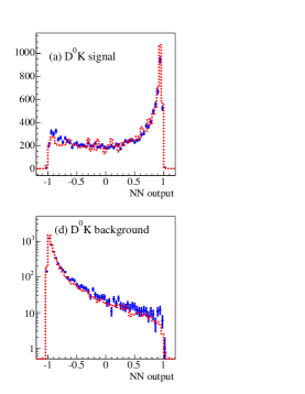
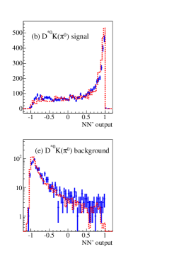
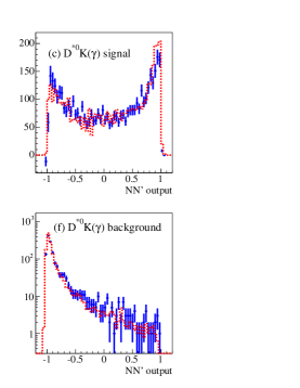
Figure 2: Distributions of the continuum suppression neural network ($NN$ and $NN^{\prime}$) outputs for the three modes. Figs. (a-c) show the expected distribution from signal events. The dashed line histogram shows the distribution of simulated signal events and the histogram with error bars shows the distribution of $D^{(*)0}\pi$ control sample events with background subtracted using the $m_{\rm ES}$ sideband (5.20 GeV $<\mbox{$m_{\rm ES}$}<$ 5.27 GeV). Figs. (d-f) show the expected distribution for continuum background events. The dashed line histogram shows the distribution of simulated continuum events and the histogram with errors shows the distribution of off-resonance events. The $m_{\rm ES}$ and $\Delta E$ requirements on the off-resonance and continuum Monte Carlo events have been kept loose to increase the statistics. Each Monte Carlo histogram is normalized to the area of the corresponding data histogram.

III.1 Basic Selection Criteria

Charged kaon and pion candidates in the decay modes of interest must satisfy $K$ or $\pi$ identification criteria PIDref that are typically 85% efficient, depending on momentum and polar angle. The misidentification rates are at the few percent level.

The invariant mass of the $K\pi$ pair must be within 18.8 MeV (2.5$\sigma$) of the mean reconstructed $D^{0}$ mass (1863.3 MeV). For modes with $\tilde{D}^{*0}\rightarrow\tilde{D}^{0}\pi^{0}$ and $\tilde{D}^{*0}\rightarrow\tilde{D}^{0}\gamma$ the mass difference $\Delta M$ between the $\tilde{D}^{*0}~{}$ and the $\tilde{D}^{0}$ must be within 3.5 MeV (3.5$\sigma$) and 13 MeV (2$\sigma$), respectively, of the expectation for $\tilde{D}^{*0}$ decays (142.2 MeV).

A major background arises from $DK$ and $D^{*}K$ decays in which the $K$ and $\pi$ in the $D$ decay are misidentified as $\pi$ and $K$, respectively. When this happens, the decay could be reconstructed as a $\kern 1.99997pt\overline{\kern-1.99997ptD}{}K$ or $\kern 1.99997pt\overline{\kern-1.99997ptD}{}^{*}K$ signal event. To eliminate this background, we recompute the invariant mass ($M_{{\rm switch}}$) of the $h^{+}h^{-}$ pair in $\tilde{D}^{0}\rightarrow h^{+}h^{-}$ switching the particle identification assumptions ($\pi$ vs. $K$) on the $h^{+}$ and the $h^{-}$. We veto any candidates with $M_{{\rm switch}}$ within 18 MeV of the known $D$ mass PDG ; this requirement is 90% efficient on signal decays. In the case of $\tilde{D}^{0}K$, we also veto any candidate for which the $\tilde{D}^{0}$ is consistent with $D^{*+}\rightarrow D^{0}\pi^{+}$ or $D^{*0}\rightarrow D^{0}\pi^{0}$ decay.

III.2 Neural Network

After these initial selection criteria, backgrounds are overwhelmingly from continuum events, especially $e^{+}e^{-}\rightarrow c\bar{c}$, with $\bar{c}\rightarrow\kern 1.99997pt\overline{\kern-1.99997ptD}{}^{0}X$, $\kern 1.99997pt\overline{\kern-1.99997ptD}{}^{0}\rightarrow K^{+}\pi^{-}$ and $c\rightarrow DX$, $D\rightarrow K^{-}Y$.

The continuum background is reduced using a neural network technique. The neural network algorithms used for the modes with and without a $D^{*}$ are slightly different. First, for all modes we use a common neural network ($NN$) based on nine quantities, listed below, that distinguish between continuum and $B\kern 1.79993pt\overline{\kern-1.79993ptB}{}$ events. Then, for the modes with a $D^{*}$ we also take advantage of the fact that the signal is distributed as $\cos^{2}\theta_{D^{*}}$ for $D^{*}\rightarrow D\pi$ or $\sin^{2}\theta_{D^{*}}$ for $D^{*}\rightarrow D\gamma$, while the background is roughly independent of $\cos\theta_{D^{*}}$. Here $\theta_{D^{*}}$ is the decay angle of the $D^{*}$, i.e., the angle between the direction of the $D$ and the line of flight of the $D^{*}$ relative to the parent $B$, evaluated in the $D^{*}$ rest frame. Thus, we construct a second neural network, $NN^{\prime}$, which takes as inputs the output of $NN$ and the value of $\cos\theta_{D^{*}}$. We then use as a selection requirement the output of $NN$ in the $\tilde{D}^{0}K$ analysis and the output of $NN^{\prime}$ in the $\tilde{D}^{*0}K$ analysis.

The nine variables used in defining $NN$ are the following:

1. A Fisher discriminant Fisher constructed from the quantities $L_{0}=\sum_{i}{p_{i}}$ and $L_{2}=\sum_{i}{p_{i}\cos^{2}\theta_{i}}$ calculated in the CM frame. Here, $p_{i}$ is the momentum and $\theta_{i}$ the angle with respect to the thrust axis of the $B$ candidate of tracks and clusters not used to reconstruct the $B$ meson.

2. $|\cos\theta_{T}|$, where $\theta_{T}$ is the angle in the CM frame between the thrust axes of the $B$ candidate and the detected remainder of the event. The distribution of $|\cos\theta_{T}|$ is approximately flat for signal and strongly peaked at one for continuum background.

3. $\cos\theta^{*}_{B}$, where $\theta^{*}_{B}$ is the polar angle of the $B$ candidate in the CM frame. In this variable, the signal follows a $\sin^{2}\theta^{*}_{B}$ distribution, while the background is approximately uniform.

4. $\cos\theta_{D}^{K}$ where $\theta_{D}^{K}$ is the decay angle in $\tilde{D}^{0}\rightarrow K\pi$.

5. $\cos\theta_{B}^{D^{(*)}}$, where $\theta_{B}^{D^{(*)}}$ is the decay angle in $B\rightarrow\tilde{D}^{0}K$ or $B\rightarrow\tilde{D}^{*0}K$. In signal events the distributions of $\cos\theta_{D}^{K}$ and $\cos\theta_{B}^{D^{(*)}}$ are uniform. On the other hand, the corresponding distributions in combinatorial background events tend to show accumulations of events near the extreme values.

6. The charge difference $\Delta Q$ between the sum of the charges of tracks in the $\tilde{D}^{0}$ or $\tilde{D}^{*0}$ hemisphere and the sum of the charges of the tracks in the opposite hemisphere excluding those tracks used in the reconstructed $B$. The partitioning of the event in the two hemispheres is done in the CM frame. For signal, $\langle\Delta Q\rangle=0$, whereas for the $c\bar{c}$ background $\langle\Delta Q\rangle\approx\frac{7}{3}\times Q_{B}$, where $Q_{B}$ is the charge of the $B$ candidate. The value of $\langle\Delta Q\rangle$ in $c\bar{c}$ events is a consequence of the correlation between the charge of the $c$ (or $\bar{c}$) in a given hemisphere and the sum of the charges of all particles in that hemisphere. Since the $\Delta Q$ RMS is 2.4, this variable provides approximately a $1\sigma$ separation between signal and $c\bar{c}$ background.

7. $Q_{B}\cdot Q_{K}$, where $Q_{K}$ is the sum of the charges of all kaons not in the reconstructed $B$, and $Q_{B}$, as defined above, is the charge of the reconstructed $B$ candidate. In many signal events, there is a charged kaon among the decay products of the other $B$ in the event. The charge of this kaon tends to be highly correlated with the charge of the $B$. Thus, signal events tend to have $Q_{B}\cdot Q_{K}\leq-1$. On the other hand, most continuum events have no kaons outside of the reconstructed $B$, and therefore $Q_{K}=0$.

8. The distance of closest approach between the bachelor track and the trajectory of the $\tilde{D}^{0}$. This is consistent with zero for signal events, but can be larger in $c\bar{c}$ events.

9. A quantity ${\cal M}_{K\ell}$ defined to be zero if there are no leptons ($e$ or $\mu$) in the event, one if there is a lepton in the event and the invariant mass ($m_{K\ell}$) of this lepton and the bachelor kaon is less than the mass of the $D$-meson ($m_{D}$), and two if $m_{K\ell}>m_{D}$. This quantity differentiates between continuum and signal events because the probability of finding a lepton in a continuum event is smaller than in a $B\kern 1.79993pt\overline{\kern-1.79993ptB}{}$ event. Furthermore, a large fraction of leptons in $c\bar{c}$ events are from $D\rightarrow K\ell\nu$, where $K$ is reconstructed as the bachelor kaon. For these events $m_{K\ell}<m_{D}$, while in signal events the expected distribution of $m_{K\ell}$ extends to larger values.

The neural networks ($NN$ and $NN^{\prime}$) are trained with simulated continuum and signal events. The distributions of the $NN$ and $NN^{\prime}$ outputs for the control samples ($D\pi$, $D^{*}\pi$, and off resonance data) are compared with expectations from the Monte Carlo simulation in Fig. 2. The agreement is satisfactory. We have also examined the distributions of all variables used in $NN$ and $NN^{\prime}$, and found good agreement between the simulation and the data control samples.

Our final event selection requirement is $NN>0.5$ for $\kern 1.99997pt\overline{\kern-1.99997ptD}{}K$ and $NN^{\prime}>0.5$ for $\kern 1.99997pt\overline{\kern-1.99997ptD}{}^{*}K$. In addition, to reduce the remaining $B\kern 1.79993pt\overline{\kern-1.79993ptB}{}$ backgrounds, we also require $\cos\theta_{D}^{K}>-0.75$. These final requirements are about 40% efficient on simulated signal events, and reject 98.5% of the continuum background.

The overall reconstruction efficiencies, estimated from Monte Carlo simulation, are about 14% for $\kern 1.99997pt\overline{\kern-1.99997ptD}{}K$, 8% for $\kern 1.99997pt\overline{\kern-1.99997ptD}{}^{*}K$ with $\kern 1.99997pt\overline{\kern-1.99997ptD}{}^{*}\rightarrow\kern 1.99997pt\overline{\kern-1.99997ptD}{}\pi^{0}$ and 7% for $\kern 1.99997pt\overline{\kern-1.99997ptD}{}^{*}K$ with $\kern 1.99997pt\overline{\kern-1.99997ptD}{}^{*}\rightarrow\kern 1.99997pt\overline{\kern-1.99997ptD}{}\gamma$. Note that a precise knowledge of the efficiencies is not needed in the analysis. We apply the identical requirements to the normalization modes $DK$ and $D^{*}K$. Then, in the extraction of ${\cal R}_{K\pi}$ and ${\cal R}_{K\pi}^{*}$, the efficiencies of the overall selection cancel in the ratio.

Table 2: Summary of fit results.

Mode	$\kern 1.99997pt\overline{\kern-1.99997ptD}{}K$	$\kern 1.99997pt\overline{\kern-1.99997ptD}{}^{*}K$, $\kern 1.99997pt\overline{\kern-1.99997ptD}{}^{*}\rightarrow\kern 1.99997pt\overline{\kern-1.99997ptD}{}\pi^{0}$	$\kern 1.99997pt\overline{\kern-1.99997ptD}{}^{*}K$, $\kern 1.99997pt\overline{\kern-1.99997ptD}{}^{*}\rightarrow\kern 1.99997pt\overline{\kern-1.99997ptD}{}\gamma$
Ratio of rates, ${\cal R}_{K\pi}$ or ${\cal R}^{*}_{K\pi}$, $\times 10^{-3}$	${\cal R}_{K\pi}=13^{+11}_{-9}$	${\cal R}^{*}_{K\pi}=-2^{+10}_{-6}$	${\cal R}^{*}_{K\pi}=11^{+18}_{-13}$
Number of signal events	$5^{+4}_{-3}$	$-0.2^{+1.3}_{-0.7}$	$1.2^{+2.1}_{-1.4}$
Number of normalization events	$368\pm 26$	$150\pm 17$	$108\pm 14$
Number of peaking charmless events	$0.7^{+1.4}_{-0.7}$	$0.0^{+0.3}_{-0.0}$	$0.1^{+0.8}_{-0.1}$
Number of peaking $D^{(*)}\pi$ events in signal sample	$0.48\pm 0.05$	$0.18\pm 0.03$	$0.01\pm 0.02$

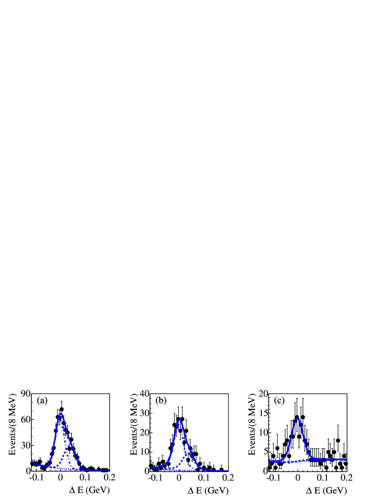
Figure 3: $\Delta E$ distributions for normalization events ($DK$ and $D^{*}K$) with $m_{\rm ES}$ within 3$\sigma$ of $m_{B}$ with the fit model overlaid. (a) $DK$ events. (b) $D^{*}K$ events with $D^{*}\rightarrow D\pi^{0}$. (c) $D^{*}K$ events with $D^{*}\rightarrow D\gamma$. The dashed (dot-dashed) lines are the contributions from $D\pi$ or $D^{*}\pi$ ($DK$ or $D^{*}K$) events. The dotted lines are the contributions from other backgrounds, and the solid line is the total.

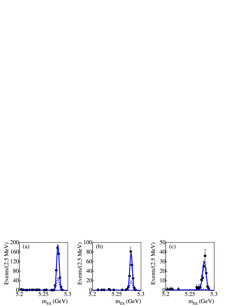
Figure 4: $m_{\rm ES}$ distributions for normalization events ($DK$ and $D^{*}K$) with $\Delta E$ in the signal region with the fit model overlaid. (a) $DK$ events. (b) $D^{*}K$ events with $D^{*}\rightarrow D\pi^{0}$. (c) $D^{*}K$ events with $D^{*}\rightarrow D\gamma$. The dashed lines represent the backgrounds; these are mostly from $D\pi$ or $D^{*}\pi$, and also peak at the $B$-mass. As explained in the text, the size of the $D\pi$ and $D^{*}\pi$ backgrounds is constrained by the simultaneous fits to the distributions of Fig. 3.

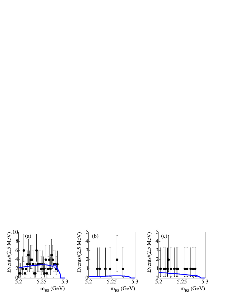
Figure 5: $m_{\rm ES}$ distributions for $\kern 1.99997pt\overline{\kern-1.99997ptD}{}K$ and $\kern 1.99997pt\overline{\kern-1.99997ptD}{}^{*}K$ events with $K\pi$ mass in a sideband of the reconstructed $D$ mass and with $\Delta E$ in the signal region. These events are used to constrain the size of possible peaking backgrounds from charmless $B$-meson decays, i.e., decays without a $D$ in the final state. The fit model is overlaid. (a) $\kern 1.99997pt\overline{\kern-1.99997ptD}{}K$ events. (b) $\kern 1.99997pt\overline{\kern-1.99997ptD}{}^{*}K$ events with $D^{*}\rightarrow D\pi^{0}$. (c) $\kern 1.99997pt\overline{\kern-1.99997ptD}{}^{*}K$ events with $D^{*}\rightarrow D\gamma$. Note that the $K\pi$ mass range in the sideband selection is a factor of 2.7 larger than in the signal selection.

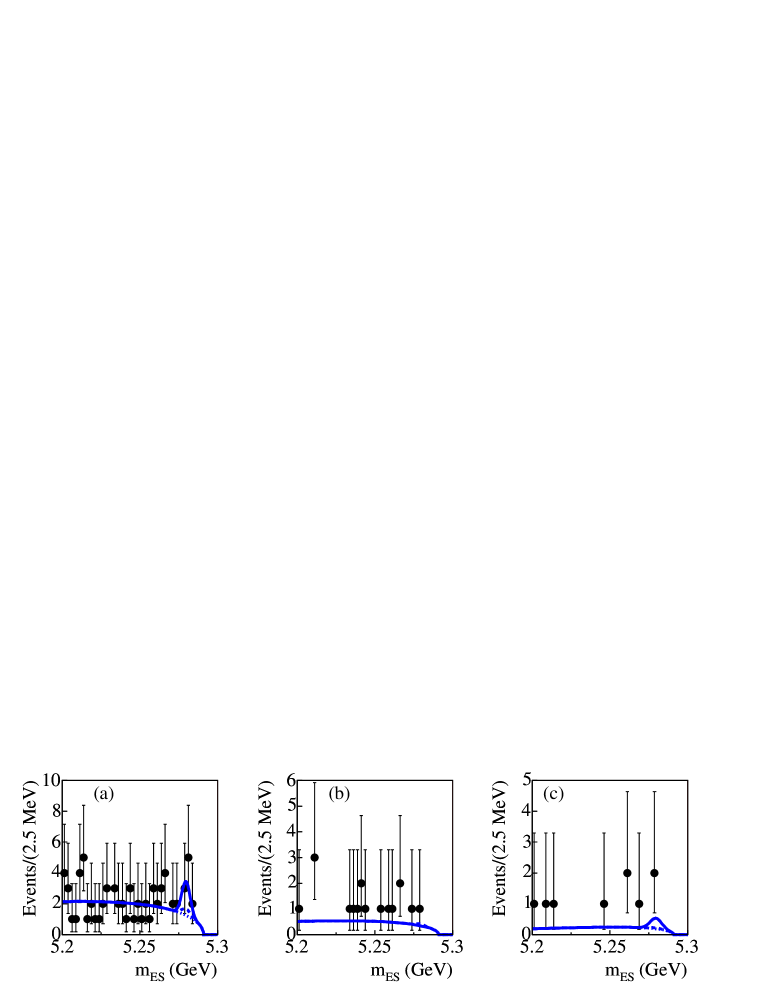
Figure 6: $m_{\rm ES}$ distributions for candidate signal events with the fit model overlaid. (a) $\kern 1.99997pt\overline{\kern-1.99997ptD}{}K$ events. (b) $\kern 1.99997pt\overline{\kern-1.99997ptD}{}^{*}K$ events with $D^{*}\rightarrow D\pi^{0}$. (c) $\kern 1.99997pt\overline{\kern-1.99997ptD}{}^{*}K$ events with $D^{*}\rightarrow D\gamma$.

III.3 Fitting for event yields and ${\cal R}^{(*)}_{K\pi}$

The ratios ${\cal R}_{K\pi}$ and ${\cal R}^{*}_{K\pi}$ are extracted from the ratios of the event yields in the $m_{ES}$ distribution for the signal modes ($\kern 1.99997pt\overline{\kern-1.99997ptD}{}K$ and $\kern 1.99997pt\overline{\kern-1.99997ptD}{}^{*}K$) and the normalization modes ($DK$ and $D^{*}K$), taking into account potential differences in efficiencies and backgrounds. All events must satisfy the requirements discussed above and have a $\Delta E$ value consistent with zero within the resolution ($-52~{}{\rm MeV}<\Delta E<44~{}{\rm MeV}$). Here we discuss the procedure to extract ${\cal R}_{K\pi}$; the values of ${\cal R}^{*}_{K\pi,D\pi^{0}}$ and ${\cal R}^{*}_{K\pi,D\gamma}$ are obtained in the same way.

The $m_{\rm ES}$ distributions for $\kern 1.99997pt\overline{\kern-1.99997ptD}{}K$ (signal mode) and $DK$ (normalization mode) are fitted simultaneously. The fit parameter ${\cal R}_{K\pi}$ is given by ${\cal R}_{K\pi}\equiv c\cdot N_{\kern 1.39998pt\overline{\kern-1.39998ptD}{}K}/N_{DK}$, where $N_{\kern 1.39998pt\overline{\kern-1.39998ptD}{}K}$ and $N_{DK}$ are the fitted yields of $\kern 1.99997pt\overline{\kern-1.99997ptD}{}K$ and $DK$ events, and $c$ is a correction factor, determined from Monte Carlo, for the ratio of efficiencies between the two modes. We find that this factor $c$ is consistent with unity within the statistical accuracy of the simulation, $c=0.98\pm 0.04$ (these correction factors are $c=0.97\pm 0.05$ and $c=0.99\pm 0.05$ for $D^{*}\rightarrow D\pi^{0}$ and $D^{*}\rightarrow D\gamma$, respectively).

The $m_{\rm ES}$ distributions are modeled as the sum of a threshold combinatorial background function ARGUS and a Gaussian lineshape centered at $m_{B}$. The parameters of the background function for the signal mode are constrained by a simultaneous fit of the $m_{\rm ES}$ distribution for events in the sideband of $\Delta E$ ($-120~{}{\rm MeV}<\Delta E<200~{}{\rm MeV}$, excluding the $\Delta E$ signal region defined above). The parameters of the Gaussian for the signal and normalization modes are taken to be identical. The number of events in the Gaussian is $N_{sig}+N_{peak}$, where $N_{sig}=N_{DK}$ or $N_{\kern 1.39998pt\overline{\kern-1.39998ptD}{}K}$ and $N_{peak}$ is the number of background events expected to be distributed in the same way as $DK$ or $\kern 1.99997pt\overline{\kern-1.99997ptD}{}K$ in $m_{\rm ES}$ (“peaking backgrounds”).

There are two classes of peaking background events:

1. Charmless $B$ decays, e.g., $B^{-}\rightarrow K^{+}K^{-}\pi^{+}$. These are indistinguishable from the $\kern 1.99997pt\overline{\kern-1.99997ptD}{}K$ signal if the $K^{-}\pi^{+}$ pair happens to be consistent with the $D$ mass.

2. Events of the type $B^{-}\rightarrow D^{0}\pi^{-}$, where the bachelor $\pi^{-}$ is misidentified as a $K^{-}$. When the $D^{0}$ decays into $K^{-}\pi^{+}$ ($K^{+}\pi^{-}$), these events are indistinguishable in $m_{\rm ES}$ from $DK$ ($\kern 1.99997pt\overline{\kern-1.99997ptD}{}K$), since $m_{\rm ES}$ is independent of particle identification assumptions.

The amount of peaking charmless $B$ background (1) is estimated directly from the data by performing a simultaneous fit to events in the sideband of the reconstructed $D$ mass. In this fit the number of charmless background events is constrained to be $\geq 0$.

The $\Delta E$ distribution of the $D\pi$ background (2) is shifted by about $+50$ MeV due to the misidentification of the bachelor $\pi$ as a $K$. Since the $\Delta E$ resolution is of order 20 MeV, the $\Delta E$ requirement does not eliminate this background completely. The remaining $D\pi$ background after the $\Delta E$ requirement is estimated relaxing the $\Delta E$ requirement and performing a fit to the $\Delta E$ distribution of the $DK$ candidate sample, as described below.

We fit the $\Delta E$ distribution of $DK$ candidates, with $m_{\rm ES}$ within $3\sigma$ of $m_{B}$, to the sum of a $DK$ component, a $D\pi$ background component, and a combinatorial background component, see Fig. 3. From this fit we can estimate the number of $D\pi$ background events after the $\Delta E$ requirement, which we denote as $N^{\pi}_{DK}$. In this fit, the $\Delta E$ shapes of the $DK$ and $D\pi$ components are constrained from the data as follows:

• The large $D\pi$ sample, with the bachelor track identified as a pion, is used to constrain the shape of the $DK$ component in the sample of $DK$ candidates.

• The same sample of $D\pi$ events, but reconstructed as $DK$ events, is used to constrain the shape of the $D\pi$ background in the $DK$ sample.

The $D\pi$ peaking background is much more important in the $DK$ (normalization) channel than in the $\kern 1.99997pt\overline{\kern-1.99997ptD}{}K$ (signal) channel. This is because in order to contribute to the signal channel, the $D^{0}$ has to decay into $K^{+}\pi^{-}$, and this mode is doubly CKM suppressed. For the $\kern 1.99997pt\overline{\kern-1.99997ptD}{}K$ (signal) sample, the contribution from the residual $D\pi$ peaking background in the $m_{\rm ES}$ fit is estimated as $N^{\pi}_{\kern 1.39998pt\overline{\kern-1.39998ptD}{}K}=r^{2}_{D}N^{\pi}_{DK}$, where $r_{D}=0.060\pm 0.002$ is the ratio of the doubly CKM-suppressed to the CKM-favored $D\rightarrow K\pi$ amplitudes and $N^{\pi}_{DK}$ was defined above.

The complete procedure simultaneously fits seven distributions: the $m_{ES}$ distributions of $DK$ and $\kern 1.99997pt\overline{\kern-1.99997ptD}{}K$, the $\kern 1.99997pt\overline{\kern-1.99997ptD}{}K$ distributions in sidebands of $\Delta E$ and $m(D^{0})$, the $\Delta E$ distribution of $DK$, and the $\Delta E$ distributions of $D\pi$ reconstructed as $D\pi$ and as $DK$. All fits are unbinned extended maximum likelihood fits. They are configured in such a way that ${\cal R}_{K\pi}$ and ${\cal R}^{*}_{K\pi}$ are explicit fit parameters. The advantage of this approach is that all uncertainties, including the uncertainties in the PDFs and the uncertainties in the background subtractions, are correctly propagated in the statistical uncertainty reported by the fit.

The fit is performed separately for $\kern 1.99997pt\overline{\kern-1.99997ptD}{}K$, $\kern 1.99997pt\overline{\kern-1.99997ptD}{}^{*}K$, $\kern 1.99997pt\overline{\kern-1.99997ptD}{}^{*}\rightarrow\kern 1.99997pt\overline{\kern-1.99997ptD}{}\pi^{0}$, and $\kern 1.99997pt\overline{\kern-1.99997ptD}{}^{*}K$, $\kern 1.99997pt\overline{\kern-1.99997ptD}{}^{*}\rightarrow\kern 1.99997pt\overline{\kern-1.99997ptD}{}\gamma$ and is identical for all three modes, except in the choice of parameterization for some signal and background components in the $\Delta E$ fits.

Systematic uncertainties in the detector efficiency cancel in the ratio. This cancellation has been verified by studies of simulated events, with a statistical precision of a few percent. The likelihood includes a Gaussian uncertainty term for this cancellation which is set by the statistical accuracy of the simulation. Other systematic uncertainties, e.g., the uncertainty in the parameter $r_{D}$ used to estimate the amount of peaking backgrounds from $D^{(*)}\pi$, are also included in the formulation of the likelihood.

The fit procedure has been extensively tested on sets of simulated events. It was found to provide an unbiased estimation of the parameters ${\cal R}_{K\pi}$ and ${\cal R}^{*}_{K\pi}$.

IV RESULTS

The results of the fits are displayed in Table 2 and Figs. 3, 4, 5, and 6. As is apparent from Fig. 6, we see no evidence for the $\kern 1.99997pt\overline{\kern-1.99997ptD}{}^{*}K$ and $\kern 1.99997pt\overline{\kern-1.99997ptD}{}K$ modes.

For the $\kern 1.99997pt\overline{\kern-1.99997ptD}{}K$ mode we find ${\cal R}_{K\pi}=(13^{+11}_{-9})\times 10^{-3}$; for the $\kern 1.99997pt\overline{\kern-1.99997ptD}{}^{*}K$ mode we find ${\cal R}^{*}_{K\pi,D\pi^{0}}=(-2^{+10}_{-6})\times 10^{-3}$ (for $D^{*}\rightarrow D\pi^{0}$) and ${\cal R}^{*}_{K\pi,D\gamma}=(11^{+18}_{-13})\times 10^{-3}$ (for $D^{*}\rightarrow D\gamma$).

Next, we use our measurements to extract information on $r_{B}$ and $r^{*}_{B}$. In the case of decays into $\tilde{D}^{*0}$ we start from equations 12 and 13 to derive

$$r_{B}^{*2}=\frac{{\cal R}^{*}_{K\pi,D\pi^{0}}+{\cal R}^{*}_{K\pi,D\gamma}}{2}-r_{D}^{2}.$$ (14)

We use the relationship given by equation 14 in conjunction with $r_{D}=0.060\pm 0.002$ and our results for ${\cal R}^{*}_{K\pi,D\pi^{0}}$ and ${\cal R}^{*}_{K\pi,D\gamma}$ to extract information on $r_{B}^{*2}$ with no assumptions on the values of $\gamma$ and strong phases.

Since the uncertainties in ${\cal R}^{*}_{K\pi,D\pi^{0}}$ and ${\cal R}^{*}_{K\pi,D\gamma}$ are non-Gaussian, care must be taken in propagating them into an uncertainty in $r_{B}^{*2}$. We interpret the fit likelihoods for ${\cal R}^{*}_{K\pi,D\pi^{0}}$ and ${\cal R}^{*}_{K\pi,D\gamma}$ (see Figure 7) as posterior PDFs assuming constant priors. We assume a Gaussian PDF for $r_{D}$. We then convolve numerically the three PDFs for ${\cal R}^{*}_{K\pi,D\pi^{0}}$, ${\cal R}^{*}_{K\pi,D\gamma}$, and $r_{D}$ according to equation 14 to obtain a PDF for $r_{B}^{*2}$ which is shown in Figure 8. The convolution relies on the fact that the measurements of ${\cal R}^{*}_{K\pi,D\pi^{0}}$ and ${\cal R}^{*}_{K\pi,D\gamma}$ are uncorrelated (the correlation due to the uncertainty in $r_{D}$, which was used to extract the $D\pi$ peaking backgrounds in the two modes, is negligible).

Our result is $r_{B}^{*2}=(4^{+14}_{-8})\times 10^{-3}$. Based on the PDF for $r_{B}^{*2}$ shown in Figure 8 we set an upper limit $r_{B}^{*2}<(0.16)^{2}$ at the 90% C.L. using a Bayesian method with a uniform prior for $r_{B}^{*2}>0$.

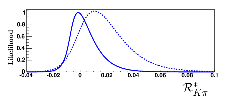
Figure 7: Likelihood functions as obtained from the fit described in the text for ${\cal R}^{*}_{K\pi,D\pi^{0}}$ (solid line) and ${\cal R}^{*}_{K\pi,D\gamma}$ (dashed line).

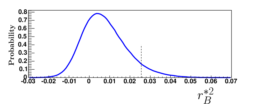
Figure 8: Probability distribution function (arbitrary units) for $r_{B}^{*2}$ obtained as described in the text. The integral of the function for $0<r_{B}^{*2}<(0.16)^{2}$ is nine-tenths of the integral for $r_{B}^{*2}>0$. The vertical dashed line is drawn at $r_{B}^{*2}=(0.16)^{2}$.

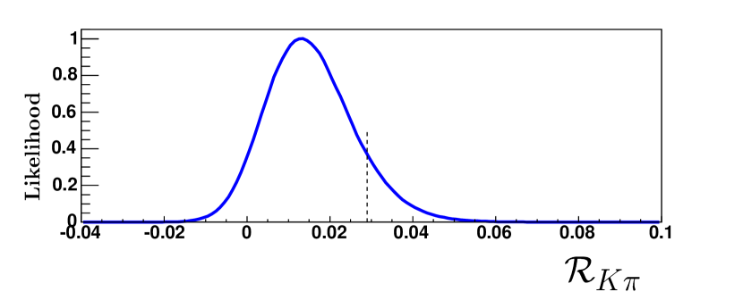
Figure 9: Likelihood function (arbitrary units) for ${\cal R}_{K\pi}$ as extracted from the fit described in the text. The integral of the likelihood function for $0<{\cal R}_{K\pi}<0.029$ is nine-tenths of the integral for ${\cal R}_{K\pi}>0$. The vertical dashed line is drawn at ${\cal R}_{K\pi}=0.029$.

In the case of decays into a $D/\kern 1.99997pt\overline{\kern-1.99997ptD}{}$, there is not enough information to extract the ratio $r_{B}$ without additional assumptions. Thus, we first extract an upper limit on the experimentally measured quantity ${\cal R}_{K\pi}$. This is done starting from the likelihood as a function of ${\cal R}_{K\pi}$ (see Fig. 9) using a Bayesian method with a uniform prior for ${\cal R}_{K\pi}>0$. The limit is ${\cal R}_{K\pi}<0.029$ at 90%C.L. Next, in Fig. 10 we show the dependence of ${\cal R}_{K\pi}$ on $r_{B}$, together with our limit on ${\cal R}_{K\pi}$. This dependence is shown allowing a $\pm 1\sigma$ variation on $r_{D}$, for the full range $0^{\circ}-180^{\circ}$ for $\gamma$ and $\delta$, as well as with the restriction $51^{\circ}<\gamma<66^{\circ}$ suggested by global CKM fits ckmfitter . We use the information displayed in this Figure to set an upper limit on $r_{B}$. The least restrictive limit on $r_{B}$ is computed assuming maximal destructive interference between the $b\rightarrow c$ and $b\rightarrow u$ amplitudes: $\gamma=0^{\circ},\delta=180^{\circ}$ or $\gamma=180^{\circ},\delta=0^{\circ}$. The limit is $r_{B}<0.23$ at 90% C.L.

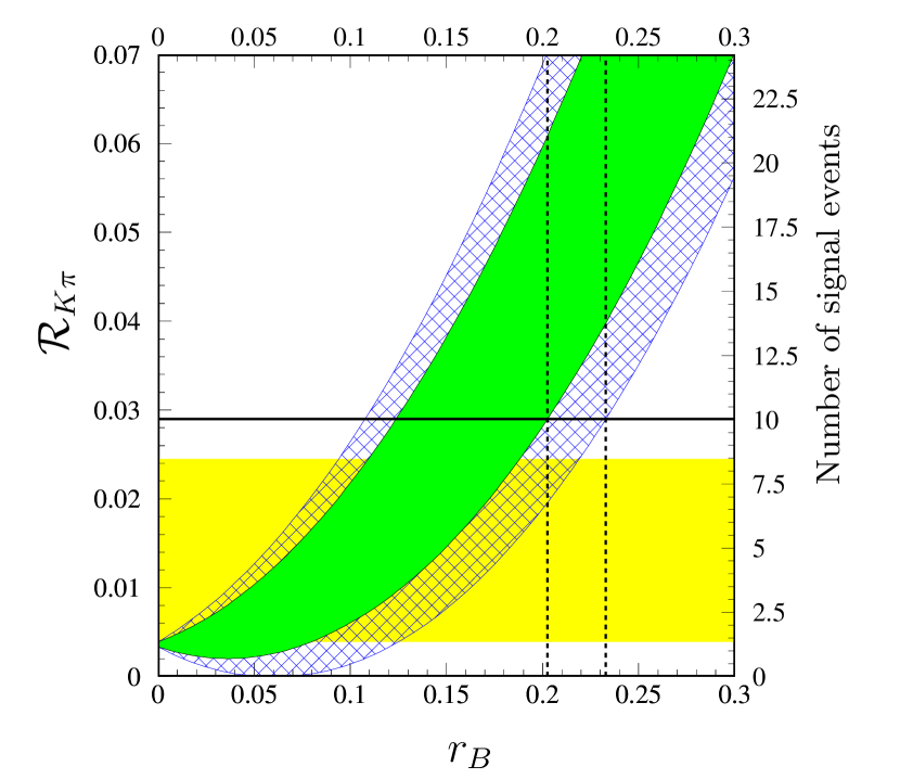
Figure 10: Expectations for ${\cal R}_{K\pi}$ and the number of signal events vs. $r_{B}$. Dark filled-in area: allowed region for any value of $\delta$, with a $\pm 1\sigma$ variation on $r_{D}$, and $51^{\circ}<\gamma<66^{\circ}$. Hatched area: additional allowed region with no constraint on $\gamma$. Note that the uncertainty on $r_{D}$ has a very small effect on the size of the allowed regions. The horizontal line represents the 90% C.L. limit ${\cal R}_{K\pi}<0.029$. The vertical dashed lines are drawn at $r_{B}=0.203$ and $r_{B}=0.233$. They represent the 90% C.L. upper limits on $r_{B}$ with and without the constraint on $\gamma$. The light filled-in area represents the 68% C.L. region corresponding to ${\cal R}_{K\pi}=0.013\pm^{0.011}_{0.009}$.

Table 3: Summary of the results of this analysis.

	Measured Value	90% C.L. limit
${\cal R}_{K\pi}$	$0.013\pm^{0.011}_{0.009}$	$<0.029$
${\cal R}^{*}_{K\pi,D\pi^{0}}$	$-0.002\pm^{0.010}_{0.006}$	$<0.023$
${\cal R}^{*}_{K\pi,D\gamma}$	$0.011\pm^{0.018}_{0.013}$	$<0.045$
$r_{B}$	…	$<0.23$
$r^{*2}_{B}$	$0.004\pm^{0.014}_{0.008}$	$<(0.16)^{2}$

V SUMMARY

In summary, we find no significant evidence for the decays $B^{\pm}\rightarrow[K^{\mp}\pi^{\pm}]_{D}K^{\pm}$ and $B^{\pm}\rightarrow[K^{\mp}\pi^{\pm}]_{D^{*}}K^{\pm}$. We set upper limits on the ratios ${\cal R}^{(*)}_{K\pi}$ of the rates for these modes and the favored modes $B^{\pm}\rightarrow[K^{\pm}\pi^{\mp}]_{D}K^{\pm}$ and $B^{\pm}\rightarrow[K^{\pm}\pi^{\mp}]_{D^{*}}K^{\pm}$. We also use our data to set upper limits on the ratios of $b\rightarrow u$ and $b\rightarrow c$ amplitudes $r_{B}$ and $r^{*}_{B}$. All of our results are summarized in Table 3.

Our results favor values of $r_{B}$ and $r_{B}^{*}$ somewhat smaller than the value of 0.2 which can be estimated from the measurements of color-suppressed $b\rightarrow c$ transitions gronau . If $r_{B}$ and $r_{B}^{*}$ are small, the suppression of the $b\rightarrow u$ amplitude will make the determination of $\gamma$ using methods based on the interference of the diagrams in Fig. 1 difficult.

VI ACKNOWLEDGMENTS

We are grateful for the extraordinary contributions of our PEP-II colleagues in achieving the excellent luminosity and machine conditions that have made this work possible. The success of this project also relies critically on the expertise and dedication of the computing organizations that support BABAR. The collaborating institutions wish to thank SLAC for its support and the kind hospitality extended to them. This work is supported by the US Department of Energy and National Science Foundation, the Natural Sciences and Engineering Research Council (Canada), Institute of High Energy Physics (China), the Commissariat à l’Energie Atomique and Institut National de Physique Nucléaire et de Physique des Particules (France), the Bundesministerium für Bildung und Forschung and Deutsche Forschungsgemeinschaft (Germany), the Istituto Nazionale di Fisica Nucleare (Italy), the Foundation for Fundamental Research on Matter (The Netherlands), the Research Council of Norway, the Ministry of Science and Technology of the Russian Federation, and the Particle Physics and Astronomy Research Council (United Kingdom). Individuals have received support from CONACyT (Mexico), the A. P. Sloan Foundation, the Research Corporation, and the Alexander von Humboldt Foundation.

References

(1)BABAR Collaboration, B. Aubert et al.,
Phys. Rev. Lett. 89, 201802 (2002); Belle Collaboration,
K. Abe et al., Phys. Rev. D66, 071102 (2002).
(2) L. Wolfenstein, Phys. Rev. Lett. 51, 1945 (1983).
(3) M. Gronau and D. Wyler, Phys. Lett. B265, 172 (1991);
M. Gronau and D. London, Phys. Lett. B253, 483 (1991).
(4) D. Atwood, I. Dunietz, and A. Soni, Phys. Rev. Lett. 78,
3257 (1997); Phys. Rev. D63, 036005 (2001).
(5) A. Bondar and T. Gershon, Phys. Rev. D70,
091503 (2004).
(6) Particle Data Group, S.
Eidelman et al., Phys. Lett. B592, 1 (2004).
(7)
See, for example,
M. Neubert and B. Stech, in Heavy Flavors, edited
by A.J. Buras and M. Lindner, World Scientific, Singapore, 1997, 2nd ed..
(8)
CLEO Collaboration, T.E. Coan et al., Phys. Rev. Lett. 88,
062001 (2002).
Belle Collaboration, K. Abe et al., Phys. Rev. Lett. 88,
052002 (2002); A. Satpathy et al., Phys. Lett. B553, 159 (2003).
BABAR Collaboration, B. Aubert et al., Phys. Rev.
D69, 032004 (2004).
(9) M. Gronau, Phys. Lett. B557, 198 (2003).
(10)BABAR Collaboration, B. Aubert et al.,
Phys. Rev. Lett. 93, 131804 (2004).
(11) Belle Collaboration, M. Saigo et al.,
Phys. Rev. Lett. 94, 091601 (2005).
(12) Belle Collaboration, A. Poluetkov
et al., Phys. Rev D70, 072003 (2004).
(13)BABAR Collaboration, B. Aubert et al.,
hep-ex/0504039, submitted to Phys. Rev. Lett.
(14)BABAR Collaboration, B. Aubert et al.,
Nucl. Instr. and Methods Phys. Res., Sect.
A479, 1 (2002).