EUROPEAN ORGANIZATION FOR NUCLEAR RESEARCH

CERN-EP/04-044

10^th August 2004

Journal version 25^th November 2004

Measurement of event shape distributions and moments
in $\mathrm{e^{+}e^{-}}\rightarrow\;$hadrons at 91–209 GeV
and a determination of $\alpha_{\mathrm{s}}$

The OPAL Collaboration

Abstract

We have studied hadronic events from $\mathrm{e^{+}e^{-}}$ annihilation data at centre-of-mass energies from 91 to 209 GeV. We present distributions of event shape observables and their moments at each energy and compare with QCD Monte Carlo models. From the event shape distributions we extract the strong coupling $\alpha_{\mathrm{s}}$ and test its evolution with energy scale. The results are consistent with the running of $\alpha_{\mathrm{s}}$ expected from QCD. Combining all data, the value of $\alpha_{\mathrm{s}}(M_{\mathrm{Z}})$ is determined to be

$$\alpha_{\mathrm{s}}(M_{\mathrm{Z}})=0.1191\pm 0.0005~{}\mathrm{(stat.)}\pm 0.0010~{}\mathrm{(expt.)}\pm 0.0011~{}\mathrm{(hadr.)}\pm 0.0044~{}\mathrm{(theo.)}\;.$$

The energy evolution of the moments is also used to determine a value of $\alpha_{\mathrm{s}}$ with slightly larger errors: $\alpha_{\mathrm{s}}(M_{\mathrm{Z}})=0.1223\pm 0.0005(\mathrm{stat.})\pm 0.0014(\mathrm{expt.})\pm 0.0016(\mathrm{hadr.})^{+0.0054}_{-0.0036}(\mathrm{theo.})$.

(Submitted to European Physical Journal C)

The OPAL Collaboration

G. Abbiendi², C. Ainsley⁵, P.F. Åkesson^3,y, G. Alexander²², J. Allison¹⁶, P. Amaral⁹, G. Anagnostou¹, K.J. Anderson⁹, S. Asai²³, D. Axen²⁷, I. Bailey²⁶, E. Barberio^8,p, T. Barillari³², R.J. Barlow¹⁶, R.J. Batley⁵, P. Bechtle²⁵, T. Behnke²⁵, K.W. Bell²⁰, P.J. Bell¹, G. Bella²², A. Bellerive⁶, G. Benelli⁴, S. Bethke³², O. Biebel³¹, O. Boeriu¹⁰, P. Bock¹¹, M. Boutemeur³¹, S. Braibant², R.M. Brown²⁰, H.J. Burckhart⁸, S. Campana⁴, P. Capiluppi², R.K. Carnegie⁶, A.A. Carter¹³, J.R. Carter⁵, C.Y. Chang¹⁷, D.G. Charlton¹, C. Ciocca², A. Csilling²⁹, M. Cuffiani², S. Dado²¹, A. De Roeck⁸, E.A. De Wolf^8,s, K. Desch²⁵, B. Dienes³⁰, M. Donkers⁶, J. Dubbert³¹, E. Duchovni²⁴, G. Duckeck³¹, I.P. Duerdoth¹⁶, E. Etzion²², F. Fabbri², P. Ferrari⁸, F. Fiedler³¹, I. Fleck¹⁰, M. Ford¹⁶, A. Frey⁸, P. Gagnon¹², J.W. Gary⁴, C. Geich-Gimbel³, G. Giacomelli², P. Giacomelli², M. Giunta⁴, J. Goldberg²¹, E. Gross²⁴, J. Grunhaus²², M. Gruwé⁸, P.O. Günther³, A. Gupta⁹, C. Hajdu²⁹, M. Hamann²⁵, G.G. Hanson⁴, A. Harel²¹, M. Hauschild⁸, C.M. Hawkes¹, R. Hawkings⁸, R.J. Hemingway⁶, G. Herten¹⁰, R.D. Heuer²⁵, J.C. Hill⁵, K. Hoffman⁹, D. Horváth^29,c, P. Igo-Kemenes¹¹, K. Ishii²³, H. Jeremie¹⁸, P. Jovanovic¹, T.R. Junk^6,i, J. Kanzaki^23,u, D. Karlen²⁶, K. Kawagoe²³, T. Kawamoto²³, R.K. Keeler²⁶, R.G. Kellogg¹⁷, B.W. Kennedy²⁰, S. Kluth³², T. Kobayashi²³, M. Kobel³, S. Komamiya²³, T. Krämer²⁵, P. Krieger^6,l, J. von Krogh¹¹, T. Kuhl²⁵, M. Kupper²⁴, G.D. Lafferty¹⁶, H. Landsman²¹, D. Lanske¹⁴, D. Lellouch²⁴, J. Letts^o, L. Levinson²⁴, J. Lillich¹⁰, S.L. Lloyd¹³, F.K. Loebinger¹⁶, J. Lu^27,w, A. Ludwig³, J. Ludwig¹⁰, W. Mader^3,b, S. Marcellini², A.J. Martin¹³, G. Masetti², T. Mashimo²³, P. Mättig^m, J. McKenna²⁷, R.A. McPherson²⁶, F. Meijers⁸, W. Menges²⁵, F.S. Merritt⁹, H. Mes^6,a, N. Meyer²⁵, A. Michelini², S. Mihara²³, G. Mikenberg²⁴, D.J. Miller¹⁵, W. Mohr¹⁰, T. Mori²³, A. Mutter¹⁰, K. Nagai¹³, I. Nakamura^23,v, H. Nanjo²³, H.A. Neal³³, R. Nisius³², S.W. O’Neale^1,∗, A. Oh⁸, M.J. Oreglia⁹, S. Orito^23,∗, C. Pahl³², G. Pásztor^4,g, J.R. Pater¹⁶, J.E. Pilcher⁹, J. Pinfold²⁸, D.E. Plane⁸, O. Pooth¹⁴, M. Przybycień^8,n, A. Quadt³, K. Rabbertz^8,r, C. Rembser⁸, P. Renkel²⁴, J.M. Roney²⁶, A.M. Rossi², Y. Rozen²¹, K. Runge¹⁰, K. Sachs⁶, T. Saeki²³, E.K.G. Sarkisyan^8,j, A.D. Schaile³¹, O. Schaile³¹, P. Scharff-Hansen⁸, J. Schieck³², T. Schörner-Sadenius^8,z, M. Schröder⁸, M. Schumacher³, R. Seuster^14,f, T.G. Shears^8,h, B.C. Shen⁴, P. Sherwood¹⁵, A. Skuja¹⁷, A.M. Smith⁸, R. Sobie²⁶, S. Söldner-Rembold¹⁶, F. Spano⁹, A. Stahl^3,x, D. Strom¹⁹, R. Ströhmer³¹, S. Tarem²¹, M. Tasevsky^8,s, R. Teuscher⁹, M.A. Thomson⁵, E. Torrence¹⁹, D. Toya²³, P. Tran⁴, I. Trigger⁸, Z. Trócsányi^30,e, E. Tsur²², M.F. Turner-Watson¹, I. Ueda²³, B. Ujvári^30,e, C.F. Vollmer³¹, P. Vannerem¹⁰, R. Vértesi^30,e, M. Verzocchi¹⁷, H. Voss^8,q, J. Vossebeld^8,h, C.P. Ward⁵, D.R. Ward⁵, P.M. Watkins¹, A.T. Watson¹, N.K. Watson¹, P.S. Wells⁸, T. Wengler⁸, N. Wermes³, G.W. Wilson^16,k, J.A. Wilson¹, G. Wolf²⁴, T.R. Wyatt¹⁶, S. Yamashita²³, D. Zer-Zion⁴, L. Zivkovic²⁴

¹School of Physics and Astronomy, University of Birmingham, Birmingham B15 2TT, UK
²Dipartimento di Fisica dell’ Università di Bologna and INFN, I-40126 Bologna, Italy
³Physikalisches Institut, Universität Bonn, D-53115 Bonn, Germany
⁴Department of Physics, University of California, Riverside CA 92521, USA
⁵Cavendish Laboratory, Cambridge CB3 0HE, UK
⁶Ottawa-Carleton Institute for Physics, Department of Physics, Carleton University, Ottawa, Ontario K1S 5B6, Canada
⁸CERN, European Organisation for Nuclear Research, CH-1211 Geneva 23, Switzerland
⁹Enrico Fermi Institute and Department of Physics, University of Chicago, Chicago IL 60637, USA
¹⁰Fakultät für Physik, Albert-Ludwigs-Universität Freiburg, D-79104 Freiburg, Germany
¹¹Physikalisches Institut, Universität Heidelberg, D-69120 Heidelberg, Germany
¹²Indiana University, Department of Physics, Bloomington IN 47405, USA
¹³Queen Mary and Westfield College, University of London, London E1 4NS, UK
¹⁴Technische Hochschule Aachen, III Physikalisches Institut, Sommerfeldstrasse 26-28, D-52056 Aachen, Germany
¹⁵University College London, London WC1E 6BT, UK
¹⁶Department of Physics, Schuster Laboratory, The University, Manchester M13 9PL, UK
¹⁷Department of Physics, University of Maryland, College Park, MD 20742, USA
¹⁸Laboratoire de Physique Nucléaire, Université de Montréal, Montréal, Québec H3C 3J7, Canada
¹⁹University of Oregon, Department of Physics, Eugene OR 97403, USA
²⁰CCLRC Rutherford Appleton Laboratory, Chilton, Didcot, Oxfordshire OX11 0QX, UK
²¹Department of Physics, Technion-Israel Institute of Technology, Haifa 32000, Israel
²²Department of Physics and Astronomy, Tel Aviv University, Tel Aviv 69978, Israel
²³International Centre for Elementary Particle Physics and Department of Physics, University of Tokyo, Tokyo 113-0033, and Kobe University, Kobe 657-8501, Japan
²⁴Particle Physics Department, Weizmann Institute of Science, Rehovot 76100, Israel
²⁵Universität Hamburg/DESY, Institut für Experimentalphysik, Notkestrasse 85, D-22607 Hamburg, Germany
²⁶University of Victoria, Department of Physics, P O Box 3055, Victoria BC V8W 3P6, Canada
²⁷University of British Columbia, Department of Physics, Vancouver BC V6T 1Z1, Canada
²⁸University of Alberta, Department of Physics, Edmonton AB T6G 2J1, Canada
²⁹Research Institute for Particle and Nuclear Physics, H-1525 Budapest, P O Box 49, Hungary
³⁰Institute of Nuclear Research, H-4001 Debrecen, P O Box 51, Hungary
³¹Ludwig-Maximilians-Universität München, Sektion Physik, Am Coulombwall 1, D-85748 Garching, Germany
³²Max-Planck-Institute für Physik, Föhringer Ring 6, D-80805 München, Germany
³³Yale University, Department of Physics, New Haven, CT 06520, USA

^a and at TRIUMF, Vancouver, Canada V6T 2A3
^b now at University of Iowa, Dept of Physics and Astronomy, Iowa, U.S.A.
^c and Institute of Nuclear Research, Debrecen, Hungary
^e and Department of Experimental Physics, University of Debrecen, Hungary
^f and MPI München
^g and Research Institute for Particle and Nuclear Physics, Budapest, Hungary
^h now at University of Liverpool, Dept of Physics, Liverpool L69 3BX, U.K.
ⁱ now at Dept. Physics, University of Illinois at Urbana-Champaign, U.S.A.
^j and Manchester University
^k now at University of Kansas, Dept of Physics and Astronomy, Lawrence, KS 66045, U.S.A.
^l now at University of Toronto, Dept of Physics, Toronto, Canada
^m current address Bergische Universität, Wuppertal, Germany
ⁿ now at University of Mining and Metallurgy, Cracow, Poland
^o now at University of California, San Diego, U.S.A.
^p now at The University of Melbourne, Victoria, Australia
^q now at IPHE Université de Lausanne, CH-1015 Lausanne, Switzerland
^r now at IEKP Universität Karlsruhe, Germany
^s now at University of Antwerpen, Physics Department,B-2610 Antwerpen, Belgium; supported by Interuniversity Attraction Poles Programme – Belgian Science Policy
^u and High Energy Accelerator Research Organisation (KEK), Tsukuba, Ibaraki, Japan
^v now at University of Pennsylvania, Philadelphia, Pennsylvania, USA
^w now at TRIUMF, Vancouver, Canada
^x now at DESY Zeuthen
^y now at CERN
^z now at DESY
^∗ Deceased

1 Introduction

Hadronic final states produced in the process $\mathrm{e^{+}e^{-}}\rightarrow\mathrm{q\overline{q}}$ are a valuable testing ground for the theory of the strong interaction in the Standard Model, Quantum Chromodynamics (QCD). The hadronic system in the energy range considered here is complex, consisting of typically 20–50 hadrons. Many “event shape” observables have been devised which provide a convenient way of characterizing the main features of such events. Analytic QCD predictions of the distributions of several of these event shape observables have been presented in the literature (see e.g. ref. [1]), and can be used to determine the crucial free parameter of QCD — the coupling strength $\alpha_{\mathrm{s}}$. These predictions describe the distributions of quarks and gluons, while the distributions of hadrons are measured in the data. In confronting the data with theory, Monte Carlo models of the hadronization process are commonly used to relate the partons and hadrons. Analytic QCD predictions have also been made for the moments of event shape distributions, whose evolution with centre-of-mass (c.m.) energy permit complementary determinations of $\alpha_{\mathrm{s}}$. The determination of $\alpha_{\mathrm{s}}$ from many different observables provides an important test of the consistency of QCD. In addition, measurements of event shape distributions have proved invaluable for testing and tuning Monte Carlo models of hadron production in $\mathrm{e^{+}e^{-}}\rightarrow\;$hadrons.

In this paper we present a coherent analysis of event shape distributions and moments using data collected by the OPAL detector at 12 c.m. energy points covering the LEP c.m. energy range of $\sqrt{s}\equiv E_{\mathrm{c.m.}}=91$–209 GeV. Results at 192–209 GeV are published for the first time here. Partial results at 91–189 GeV have been published by OPAL previously [2, 3, 4, 5]; these are superseded by the present measurements in order that the data at all energies can be analysed and interpreted in a consistent manner. The results presented here use identical analysis procedures throughout, and some event shape observables are included for the first time. In several cases, improved theoretical calculations are now available, as described in Sect. 4. The results at 91 GeV are based on calibration data taken during the LEP II running period (the period from 1996 onwards when LEP operated well above the $\mathrm{Z}$ mass); these share the same detector configuration (slightly different from that used in the earlier LEP I phase when LEP operated close to the $\mathrm{Z}$ peak) and reconstruction code as the higher energy data, which means that we can compare results over a wide energy range with minimal systematic differences between energies. Similar results from other LEP collaborations can be found in refs. [6, 7, 8, 9, 10, 11, 12, 13, 14, 15]. Another recent OPAL paper [16] uses the same data sample as the present study to measure jet rates.

The structure of the paper is as follows. In Sect. 2 we give a brief description of the OPAL detector, and in Sect. 3 we summarize the data and Monte Carlo samples used. The theoretical background to the work is outlined in Sect. 4. The experimental analysis techniques are explained in Sect. 5 before the measurements are presented and compared with theory in Sect. 6.

2 The OPAL detector

The OPAL detector was operated at the LEP $\mathrm{e^{+}e^{-}}$ collider at CERN from 1989 to 2000. A detailed description can be found in ref. [17]. The analysis presented here relies mainly on the measurements of momenta and directions of charged particles in the tracking chambers and of energy deposited in the electromagnetic calorimeters of the detector.

All tracking systems were located inside a solenoidal magnet which provided a uniform axial magnetic field of 0.435 T along the beam axis. The magnet was surrounded by a lead glass electromagnetic calorimeter and a hadron calorimeter of the sampling type. Outside the hadron calorimeter, the detector was surrounded by a system of muon chambers. There were similar layers of detectors in the forward and backward endcaps.

The main tracking detector was the central jet chamber. This device was approximately 4 m long and had an outer radius of about 1.85 m. It had 24 sectors with radial planes of 159 sense wires spaced by 1 cm. The electromagnetic calorimeters in the barrel and the endcap sections of the detector consisted of 11704 lead glass blocks with a depth of $24.6$ radiation lengths in the barrel and more than $22$ radiation lengths in the endcaps.

3 Data and Monte Carlo samples

The data used here were recorded from 1995–2000 using the OPAL detector at LEP. In 1995 the LEP c.m. energy was increased above the vicinity of the $\mathrm{Z}$ peak in runs at $E_{\mathrm{c.m.}}=130$ and 136 GeV. By 2000, the maximum c.m. energy had reached 209 GeV. All of the data recorded above the $\mathrm{Z}$ peak are analysed in the present study. In addition, interspersed at various points during the high energy LEP running, calibration runs were taken on the $\mathrm{Z}$ peak, at $\sqrt{s}=91.3$ GeV. These data were recorded with identical detector configuration and performance, and reconstructed with the same code, as the high energy data. For the purpose of analysis, the data have been grouped into small energy ranges, which are often merged into larger ranges for clarity of presentation. Table 1 summarizes the c.m. energy points used, the integrated luminosities at each point and the numbers of events employed for analysis after the selection described in Sect. 5.1.

Samples of Monte Carlo simulated events were used to correct the data for experimental acceptance, efficiency and backgrounds. The process $\mathrm{e^{+}e^{-}}\rightarrow\mathrm{q\overline{q}}$ was simulated using JETSET 7.4 [18] at $\sqrt{s}=91.2$ GeV, and at higher energies using $\mathcal{KK}$2f 4.01 or $\mathcal{KK}$2f 4.13 [19] with fragmentation performed using PYTHIA 6.150 or PYTHIA 6.158 [18]. Corresponding samples using HERWIG 6.2[20] or $\mathcal{KK}$2f with HERWIG 6.2 fragmentation were used for systematic checks. Four-fermion background processes were simulated using grc4f 2.1 [21] or KORALW 1.42 [22] with grc4f [21] matrix elements and with fragmentation performed using PYTHIA. The above samples, generated at each energy point studied, were processed through a full simulation of the OPAL detector [23], and reconstructed in the same way as real data. In addition, for comparisons with the corrected data, and when correcting for the effects of fragmentation, large samples of generator-level Monte Carlo events were employed, using the parton shower models PYTHIA 6.158, HERWIG 6.2 and ARIADNE 4.11[24]. Each of these fragmentation models contains a number of tunable parameters; these were adjusted by tuning to previously published OPAL data at $\sqrt{s}\sim 91$ GeV as described in ref. [25] for PYTHIA/JETSET and in ref. [26] for HERWIG and ARIADNE.

4 Theoretical background

4.1 Event shape observables

The properties of hadronic events may be described by a set of event shape observables. These may be used to characterize the distribution of particles in an event as “pencil-like”, planar, spherical, etc. They can be computed either using the measured charged particles and calorimeter clusters, or using the true hadrons or partons in simulated events. The following event shapes are considered here:

Thrust $T$:

defined by the expression[27, 28]

$$T=\max_{\vec{n}}\left(\frac{\sum_{i}|p_{i}\cdot\vec{n}|}{\sum_{i}|p_{i}|}\right)\;,$$ (1)

where $p_{i}$ is the three-momentum of particle $i$ and the summation runs over all particles, which may be the measured particles, or the true hadrons or partons in Monte Carlo events. The thrust axis $\vec{n}_{T}$ is the direction $\vec{n}$ which maximises the expression in parentheses. A plane through the origin and perpendicular to $\vec{n}_{T}$ divides the event into two hemispheres $H_{1}$ and $H_{2}$.

Thrust major $T_{\mathrm{maj.}}$:

The maximization in equation (1) is performed subject to the constraint that $\vec{n}$ must lie in the plane perpendicular to $\vec{n}_{T}$. The resulting vector is called $\vec{n}_{T_{\mathrm{maj.}}}$.

Thrust minor $T_{\mathrm{min.}}$:

The expression in parentheses in equation (1) is evaluated for the vector $\vec{n}_{T_{\mathrm{min.}}}$ which is perpendicular to both $\vec{n}_{T}$ and $\vec{n}_{T_{\mathrm{maj.}}}$.

Oblateness $O$:

This observable is defined by $O=T_{\mathrm{maj.}}-T_{\mathrm{min.}}$ [29].

Sphericity $S$ and Aplanarity $A$:

These observables are based on the momentum tensor

$$S^{\alpha\beta}=\frac{\sum_{i}p_{i}^{\alpha}p_{i}^{\beta}}{\sum_{i}p_{i}^{2}}\;,\;\;\;\alpha,\beta=1,2,3\;,$$ (2)

where the sum runs over particles, $i$, and $\alpha$ and $\beta$ denote the cartesian coordinates of the momentum vector. The three eigenvalues $Q_{j}$ of $S^{\alpha\beta}$ are ordered such that $Q_{1}<Q_{2}<Q_{3}$. These then define $S$ [30, 31] and $A$ [32] by

$$S=\frac{3}{2}(Q_{1}+Q_{2})\;\;\;\mathrm{and}\;\;\;A=\frac{3}{2}Q_{1}\;.$$ (3)

$C$- and $D$-parameters:

The momentum tensor $S^{\alpha\beta}$ is modified to become

$$\Theta^{\alpha\beta}=\frac{\sum_{i}(p_{i}^{\alpha}p_{i}^{\beta})/|p_{i}|}{\sum_{i}|p_{i}|}\;\;\;,\;\;\;\alpha,\beta=1,2,3\;.$$ (4)

The three eigenvalues $\lambda_{j}$ of this tensor define $C$[33] through

$$C=3(\lambda_{1}\lambda_{2}+\lambda_{2}\lambda_{3}+\lambda_{3}\lambda_{1})\;$$ (5)

and $D$ through

$$D=27\lambda_{1}\lambda_{2}\lambda_{3}\;.$$ (6)

Jet Masses $M_{\mathrm{H}}$ and $M_{\mathrm{L}}$:

The hemisphere invariant masses are calculated using the particles in the two hemispheres $H_{1}$ and $H_{2}$. We define $M_{\mathrm{H}}$ [34, 35] as the heavier mass, divided by $\sqrt{s}$, and $M_{\mathrm{L}}$ as the lighter mass, likewise divided by $\sqrt{s}$.

Jet Broadening observables $B_{\mathrm{T}}$, $B_{\mathrm{N}}$ and $B_{\mathrm{W}}$:

These are defined by computing the quantity

$$B_{k}=\left(\frac{\sum_{i\in H_{k}}|p_{i}\times\vec{n}_{T}|}{2\sum_{i}|p_{i}|}\right)$$ (7)

for each of the two event hemispheres, $H_{k}$, defined above. The three observables [36] are defined by

$$B_{\mathrm{T}}=B_{1}+B_{2}\;,\;\;B_{\mathrm{N}}=\min(B_{1},B_{2})\;\;\;\mathrm{and}\;\;\;B_{\mathrm{W}}=\max(B_{1},B_{2})\;$$ (8)

where $B_{\mathrm{T}}$ is the total, $B_{\mathrm{N}}$ is the narrow and $B_{\mathrm{W}}$ is the wide jet broadening.

Transition value between 2 and 3 jets $y^{\mathrm{D}}_{23}$:

The value of the jet resolution parameter, $y_{\mathrm{cut}}$, at which the event makes a transition between a 2-jet and a 3-jet assignment, for the Durham jet finding scheme [37].

In the following discussion, whenever we wish to refer to a generic event shape observable we use the symbol $y$. In almost all cases, larger values of $y$ indicate regions dominated by the radiation of hard gluons and small values of $y$ indicate the region influenced by multiple soft gluon radiation. Note that thrust $T$ forms an exception to this rule, as the value of $T$ reaches unity for events consisting of two collimated back-to-back jets. We therefore use $y=1-T$ instead.

For all of these event shapes, a perfectly collimated (“pencil-like”) two-jet final state will have $y=0$. $\mathcal{O}(\alpha_{\mathrm{s}})$ QCD processes generate planar $\mathrm{q\overline{q}}\mathrm{g}$ configurations; for most of the observables, these processes will generate contributions at $y\neq 0$ — these are sometimes referred to as “three-jet” observables. However, five of the observables ($T_{\mathrm{min.}}$, $M_{\mathrm{L}}$, $B_{\mathrm{N}}$, $D$ and $A$), are still zero at $\mathcal{O}(\alpha_{\mathrm{s}})$, i.e. for planar events, and receive their leading contributions at $\mathcal{O}(\alpha_{\mathrm{s}}^{2})$ — these are referred to as “four-jet” observables.

4.2 QCD predictions for event shape distributions

QCD perturbation theory may be used to make predictions for event shape observables [1]. In order that these predictions be reliable, it is necessary that the value of the observable be infra-red stable (i.e. unaltered under the emission of soft gluons) and collinear stable (i.e. unaltered under collinear parton branchings).

The QCD matrix elements in $\mathrm{e^{+}e^{-}}$ annihilations are fully known to $\mathcal{O}(\alpha_{\mathrm{s}}^{2})$ [38], i.e. to next-to-leading order (NLO) for those observables dominated by three parton final states. In the two-jet (low $y$) region, however, the effect of soft and collinear emissions introduces large logarithmic effects depending on $L=\log(1/y)$, such that the leading dependence on $\alpha_{\mathrm{s}}$ and $L$ at each order, $n$, is proportional to $\alpha_{\mathrm{s}}^{n}L^{n+1}$. For six of the three-jet observables studied here ($(1-T)$, $M_{\mathrm{H}}$, $B_{\mathrm{T}}$, $B_{\mathrm{W}}$, $C$ and $y^{\mathrm{D}}_{23}$), these large logarithms can be resummed to next-to-leading order, referred to as the next-to-leading-logarithmic approximation (NLLA). The most complete QCD predictions come from combining the $\mathcal{O}(\alpha_{\mathrm{s}}^{2})$ and NLLA predictions, taking care not to double count those terms which are in common between them. Further details may be found in ref. [39, 2], and only a brief outline of the procedure is given below.

The QCD calculations make predictions for the cumulative cross-section

$$R(y)\equiv\int_{0}^{y}\frac{1}{\sigma}\frac{\mathrm{d}\sigma}{\mathrm{d}y}\mathrm{d}y$$ (9)

which take the following form for the NLLA calculations [40, 42, 41, 43]:

$$R_{\mathrm{NLLA}}(y)=(1+C_{1}\overline{\alpha}_{\mathrm{s}}+C_{2}\overline{\alpha}_{\mathrm{s}}^{2})\exp[Lg_{1}(\alpha_{\mathrm{s}}L)+g_{2}(\alpha_{\mathrm{s}}L)]\;\;,$$ (10)

where for brevity we write $\overline{\alpha}_{\mathrm{s}}$ for $(\alpha_{\mathrm{s}}/2\pi)$. The corresponding formula for the $\mathcal{O}(\alpha_{\mathrm{s}}^{2})$ prediction is:

$$R_{\mathcal{O}(\alpha_{\mathrm{s}}^{2})}(y)=1+\mathcal{A}(y)\overline{\alpha}_{\mathrm{s}}+\mathcal{B}(y)\overline{\alpha}_{\mathrm{s}}^{2}\;\;.$$ (11)

For the analysis presented here, the “$\log(R)$” matching scheme [40] is adopted for combining the $\mathcal{O}(\alpha_{\mathrm{s}}^{2})$ and NLLA predictions. This matching scheme involves taking the logarithm of equation (11) and expanding as a power series, yielding:

$$\ln R_{\mathcal{O}(\alpha_{\mathrm{s}}^{2})}(y)=\mathcal{A}(y)\overline{\alpha}_{\mathrm{s}}+\left[\mathcal{B}(y)-\frac{1}{2}\mathcal{A}(y)^{2}\right]\overline{\alpha}_{\mathrm{s}}^{2}+\mathcal{O}(\alpha_{\mathrm{s}}^{3})\;\;,$$ (12)

and similarly rewriting equation (10) as:

$$\ln R_{\mathrm{NLLA}}(y)=Lg_{1}(\alpha_{\mathrm{s}}L)+g_{2}(\alpha_{\mathrm{s}}L)+C_{1}\overline{\alpha}_{\mathrm{s}}+[C_{2}-\frac{1}{2}C_{1}^{2}]\overline{\alpha}_{\mathrm{s}}^{2}+\mathcal{O}(\alpha_{\mathrm{s}}^{3})\;\;.$$ (13)

In the $\log(R)$ matching scheme the terms up to $\mathcal{O}(\alpha_{\mathrm{s}}^{2})$ in the NLLA expression, equation (13), are replaced by the $\mathcal{O}(\alpha_{\mathrm{s}}^{2})$ terms from equation (12).

Both the $\mathcal{O}(\alpha_{\mathrm{s}}^{2})$ and NLLA QCD predictions depend on the choice of renormalization scale, $\mu$ (see ref. [1] for example). The renormalization scale factor is defined as $x_{\mu}=\mu/E_{\mathrm{c.m.}}$ where $\alpha_{\mathrm{s}}(\mu)$ is the expansion parameter which appears in the NLO perturbative predictions above. Naïvely $\mu$ would be expected to be of order of, but not necessarily equal to, $E_{\mathrm{c.m.}}$. A QCD calculation to all orders should be independent of $x_{\mu}$, but a truncated fixed order calculation does in general depend on $x_{\mu}$. For example, in the $\mathcal{O}(\alpha_{\mathrm{s}}^{2})$ calculation, the second order coefficient $\mathcal{B}(y)$ has to be replaced by $\mathcal{B}(y)+\beta_{0}\ln x_{\mu}\mathcal{A}(y)$ where $\beta_{0}=11-\frac{2}{3}n_{\mathrm{F}}$ is the leading order $\beta$-function coefficient of the renormalization group equation and $n_{\mathrm{F}}=5$ is the number of active quark flavours. Similar modifications apply to the NLLA calculations. In addition, the theoretical cross-sections are usually normalized to the Born cross-section $\sigma_{0}$ while the experimental distributions are normalized to the total hadronic cross-section, $\sigma_{\mathrm{tot.}}$, which itself depends on $\alpha_{\mathrm{s}}$:

$$\sigma_{\mathrm{tot.}}=\sigma_{0}\left(1+\frac{\alpha_{\mathrm{s}}}{\pi}\right)+\mathcal{O}(\alpha_{\mathrm{s}}^{2})$$ (14)

and this is taken into account by means of the replacement $\mathcal{B}(y)\rightarrow\mathcal{B}(y)-2\mathcal{A}(y)$.

The analysis of $\alpha_{\mathrm{s}}$ presented in this paper incorporates several improvements in the theoretical calculations and errors compared with previous determinations by OPAL based on NLLA+$\mathcal{O}(\alpha_{\mathrm{s}}^{2})$ QCD. The principal changes are as follows:

• Improvements have been made in the NLLA theory predictions for the jet broadenings $B_{\mathrm{T}}$ and $B_{\mathrm{W}}$ (ref. [41] superseding ref. [44]), and for $y^{\mathrm{D}}_{23}$ (ref. [42], superseding ref. [45], which was in turn an improvement on ref. [46]).

• The NLLA calculations for the $C$-parameter [43] were not available at the time of the earliest OPAL publications.

• The NLLA resummations do not automatically force each event shape distribution to vanish at the edge of phase space; missing subleading terms can result in a non-zero prediction outside the kinematically allowed range of the observable. A remedy for this situation involves the substitution

  $$L=\ln\left(\frac{1}{y}\right)\;\to\;\widetilde{L}=\ln\left(\frac{1}{y}-\frac{1}{y_{\mathrm{max}}}+1\right)\;.$$ (15)

  This method [40] was known at the time of the original OPAL LEP I  analysis [2], and was investigated as an alternative to the unmodified NLLA prediction. However, this is the first time it has been adopted as the standard for $\alpha_{\mathrm{s}}$ measurements by the OPAL Collaboration.

• The fixed order coefficients $\mathcal{A}(y)$ and $\mathcal{B}(y)$ are now computed using the EVENT2 Monte Carlo program [47]. This superseded an earlier program, EVENT [48]. Although both programs are based on the same $\mathcal{O}(\alpha_{\mathrm{s}}^{2})$ matrix elements from ref. [38], EVENT2 includes an improved algorithm to handle cancellations between real and virtual processes, and therefore permits a more precise determination of the coefficients.

• A more sophisticated technique for assessing the theoretical errors associated with missing higher order terms in the theory has been adopted, based on the extensive studies carried out within the LEP QCD working group [39]; see Sect. 5.3 for further details.

The theoretical calculations described above provide predictions of parton-level distributions, i.e. distributions of quarks and gluons. In contrast, the data are corrected to the hadron-level, i.e. they correspond to the distributions of the stable particles (including photons and both charged and neutral leptons) in the event as explained in Sect. 5.2. In order to confront the theory with the hadron-level data, it is necessary to correct the theory for the effects of soft fragmentation and hadronization. This was done using large samples of events (typically $10^{7}$ events) generated using the parton-shower Monte Carlo programs PYTHIA (used by default), HERWIG and ARIADNE (used for systematic error estimates). The analytical theoretical predictions for the cumulative distribution $R(y)$ were multiplied by the Monte Carlo prediction for the ratio of $R(y)$ at hadron-level to $R(y)$ at parton-level.

4.3 QCD predictions for event shape moments

The moments of the distribution of an event shape observable $y$ are defined by

$$\mbox{$\langle y^{n}\rangle$}=\int_{0}^{y_{\mathrm{max}}}y^{n}\frac{1}{\sigma}\frac{\mathrm{d}\sigma}{\mathrm{d}y}\mathrm{d}y\;,$$ (16)

where $y_{\mathrm{max}}$ is the kinematically allowed upper limit of the observable. The calculations always involve a full integration over phase space, which implies that comparison with data always probes all of the available phase space. This is in contrast to QCD predictions for distributions; these are commonly only compared with data in restricted regions, where the theory is able to describe the data well. Comparisons of QCD predictions for moments of event shape distributions with data are thus complementary to tests of the theory using the differential distributions.

The formula for the $\mathcal{O}(\alpha_{\mathrm{s}}^{2})$ QCD prediction of $\langle y^{n}\rangle$ is

$$\mbox{$\langle y^{n}\rangle$}={\cal A}_{n}\overline{\alpha}_{\mathrm{s}}+{\cal B}_{n}\overline{\alpha}_{\mathrm{s}}^{2}$$ (17)

involving the $\mathcal{O}(\alpha_{\mathrm{s}})$ coefficients ${\cal A}_{n}$ and $\mathcal{O}(\alpha_{\mathrm{s}}^{2})$ coefficients ${\cal B}_{n}$. The values of the coefficients ${\cal A}_{n}$ and ${\cal B}_{n}$ can be obtained in the same way as described above by running EVENT2. The renormalization scale dependence and correction to $\sigma_{\mathrm{tot.}}$ is implemented in the same way as described above for distributions.

The QCD predictions were transformed from the parton- to the hadron-level by multiplying by the ratio of Monte Carlo predictions for the values of moments at the hadron- and parton-level. As for the distributions, PYTHIA was used as the standard with HERWIG and ARIADNE employed for the estimation of systematic errors.

5 Analysis methods

5.1 Selection of events

The selection of events for this analysis consists of three main stages: the identification of hadronic event candidates, the removal of events with a large amount of initial-state radiation (ISR) for events at 130 GeV and above, and the removal of four-fermion background events for events above 160 GeV, i.e. above the $\mathrm{W^{+}W^{-}}$ production threshold.

The selection of hadronic events was based on simple cuts on event multiplicity (to remove leptonic final states) and on visible energy and longitudinal momentum balance (to remove two-photon events). The cuts used at 91 GeV are documented in ref. [49], while those used for higher c.m. energies have reoptimized cut parameters, as described in ref. [50]. Those parts of the OPAL detector crucial for the present analysis (electromagnetic calorimeter, jet chamber and trigger system) were required to be fully operational.

Standard criteria were used to select good tracks and calorimeter energy clusters for subsequent analysis. Charged particle tracks were required to have at least 40 hits in the jet chamber, and at least 50% of the maximum possible number of hits given the polar angle of the track. The momentum transverse to the beam axis was required to be at least 0.15 GeV. Furthermore, the point of closest approach of the track to the collision axis was required to be less than 2 cm from the nominal collision point in the $x$-$y$ plane and less than 25 cm in the $z$-direction. Energy clusters in the electromagnetic calorimeter were required to have energies exceeding 0.10 GeV (0.25 GeV) in the barrel (endcap) region of the detector. The number of good charged particle tracks was required to be greater than six. After the above cuts the $\tau^{+}\tau^{-}$ and two-photon background was negligible. Furthermore the polar angle of the thrust axis was required to satisfy $|\cos\theta_{\mathrm{T}}|<0.9$ in order that the events be well contained in the detector acceptance.

At energies significantly above $M_{\mathrm{Z}}$, the process of “radiative return” to the $\mathrm{Z}$ is a common occurrence. In order to study the properties of hadronic events at a well-defined energy scale, it is necessary to eliminate events in which a large amount of energy has been lost to ISR. The effective centre-of-mass energy after ISR, $\sqrt{s^{\prime}}$, was estimated for each selected event using the algorithm described in ref. [50]. At c.m. energies of 130 GeV and above, we demanded that $\sqrt{s}-\sqrt{s^{\prime}}<10$ GeV in order to select a sample of predominantly non-radiative events.

At energies above the $\mathrm{W^{+}W^{-}}$ production threshold, four-fermion events, especially those involving $\mathrm{q\overline{q}}$$\mathrm{q\overline{q}}$ final states, become a substantial background. These are reduced by using the standard OPAL $\mathrm{W^{+}W^{-}}$ selection procedure, which is based on a relative likelihood method [51]. The same likelihood technique has been applied at each c.m. energy studied, with the underlying reference distributions used as inputs to the likelihood calculation recomputed for each energy or range of energies. At c.m. energies of 161 GeV and above, the $\mathrm{q\overline{q}}$$\mathrm{q\overline{q}}$ likelihood was required to satisfy $\mathcal{L}_{\mathrm{q\overline{q}}\mathrm{q\overline{q}}}<0.25$ and the $\mathrm{q\overline{q}}$$\ell\nu$ likelihood was required to satisfy $\mathcal{L}_{\mathrm{q\overline{q}}\ell\nu}<0.5$.

After applying the above cuts, the numbers of selected non-radiative $\mathrm{q\overline{q}}$ candidate events were as given in Table 1, and were consistent with expectations based on Monte Carlo simulated events. After all cuts, the acceptance for non-radiative $\mathrm{q\overline{q}}$ events (defined for this purpose as those having $\sqrt{s}-\sqrt{s^{\prime}}<1$ GeV) ranged from 88.5% at 91 GeV (where the loss in acceptance is largely geometrical, arising from the $|\cos\theta_{\mathrm{T}}|<0.9$ requirement) to 76.5% at 207 GeV. The residual four-fermion background was negligible below 161 GeV, and otherwise increased from 2.1% at 161 GeV to 6.2% at 207 GeV.

5.2 Correction procedure

For each accepted event, the value of each of the event shape observables was computed. In order to mitigate the effects of double counting of energy in tracking and calorimetry, a standard algorithm was adopted which associated charged particle tracks with calorimeter clusters, and subtracted the estimated contribution of the charged particles from the calorimeter energy. All selected tracks, and the electromagnetic calorimeter clusters remaining after this procedure, were used in the evaluation of event shapes. The event shapes were then formed into histograms at each c.m. energy point. In the cases where data at more than one c.m. energy were combined (e.g. 130 and 136 GeV), the data were simply summed, and corresponding Monte Carlo samples were created by combining samples generated at each energy weighted to correspond to the integrated luminosities in data.

The expected number of residual four-fermion background events, $b_{i}$, was then subtracted from the number of data events, $N_{i}$, in each bin, $i$, of each distribution. The effects of detector acceptance and resolution and of residual ISR were then accounted for by a simple bin-by-bin correction procedure. For this procedure to be valid, it is necessary that the Monte Carlo model give a good description of the data and that the bin size be sufficiently large that bin-to-bin migration is reasonably small and symmetric; these conditions are sufficiently well satisfied for the present analysis. Two event shape distributions were formed for Monte Carlo simulated $\mathrm{q\overline{q}}$ events; the first, at the detector-level, treated the Monte Carlo identically to the data, while the second, at the hadron-level, was computed using the true momenta of the stable particles in the event, and was restricted to events whose true $s^{\prime}$ satisfied $\sqrt{s}-\sqrt{s^{\prime}}<1$ GeV. The ratio of the hadron-level to the detector-level for each bin, $\alpha_{i}$, was used as a correction factor for the data, yielding the corrected bin content $\widetilde{N}_{i}=\alpha_{i}(N_{i}-b_{i})$. This corrected hadron-level distribution was then normalized to unity: $P_{i}=\widetilde{N}_{i}/N$, where the sum $N=\sum_{k}\widetilde{N}_{k}$ includes any underflow and overflow bins. Finally, the differential distribution $R^{\prime}(y)$ was computed by dividing $P_{i}$ by the bin width. The covariance matrix $V$ for $P_{i}$ was computed by transforming the diagonal Poisson covariance matrix for the uncorrected data $N_{i}$:

$$V_{ij}=\sum_{k}\frac{\partial P_{i}}{\partial N_{k}}\frac{\partial P_{j}}{\partial N_{k}}N_{k}=\frac{1}{N^{4}}\sum_{k}\alpha_{k}^{2}N_{k}\left(N\delta_{ik}-\widetilde{N}_{i}\right)\left(N\delta_{jk}-\widetilde{N}_{j}\right)\;.$$ (18)

By setting $\alpha_{i}=1$ and $b_{i}=0$, i.e. $N_{i}=\widetilde{N}_{i}$, one may obtain the familiar expression for the covariance matrix of a multinomial distribution.

The moments were calculated by accumulating sums over all selected events:

$$N\mbox{$\langle y^{n}\rangle$}=\sum_{i=1}^{N}y_{i}^{n}\;\;,$$ (19)

where $N$ is the number of events. These sums were corrected by subtracting the background contribution estimated from simulated events. Then the correction for experimental and ISR effects was performed by multiplying by a detector correction coefficient obtained by taking the ratio of the moments at the detector and the hadron-level using simulated signal events. The statistical errors of the moments were calculated at the detector-level including the effects of Monte Carlo statistics and were subjected to the same detector correction.

5.3 Systematic uncertainties

Contributions to the systematic uncertainties affecting the corrected hadron-level distributions and moments in data were estimated by repeating the analysis with varied cuts or procedures. In each case, the difference in each bin (or for each moment) with respect to the standard analysis was taken as a contribution to the systematic error.

• The containment cut was tightened to $|\cos\theta_{\mathrm{T}}|<0.7$.

• The algorithm to compute $s^{\prime}$ was replaced by a simpler version in which at most one initial state photon was accounted for.

• The event shapes were computed using all tracks and electromagnetic calorimeter clusters. The effects of double counting are then fully taken into account through the detector correction procedure.

• The bin-by-bin corrections, $\alpha_{i}$, were computed using HERWIG instead of PYTHIA as the Monte Carlo hadronization model.

• The cut on the $\mathrm{q\overline{q}}$$\mathrm{q\overline{q}}$ four fermion likelihood was tightened to $\mathcal{L}_{\mathrm{q\overline{q}}\mathrm{q\overline{q}}}<0.1$ and loosened to $\mathcal{L}_{\mathrm{q\overline{q}}\mathrm{q\overline{q}}}<0.4$; the larger change resulting was taken to be a systematic error.

• The cut on the $\mathrm{q\overline{q}}$$\ell\nu$ four fermion likelihood was tightened to $\mathcal{L}_{\mathrm{q\overline{q}}\ell\nu}<0.25$ and loosened to $\mathcal{L}_{\mathrm{q\overline{q}}\ell\nu}<0.75$; the larger change resulting was taken to be a systematic error.

• The total four fermion background was varied by $\pm 5\%$.

The various contributions above, together with the statistical error on the correction factors arising from limited Monte Carlo statistics, were summed in quadrature to form the systematic error. None of these sources of systematic error is dominant, but typically the larger contributions arise from the use of HERWIG and the use of all tracks and clusters. In addition, at high $E_{\mathrm{c.m.}}$ and high $y$, the variation of the $\mathcal{L}_{\mathrm{q\overline{q}}\mathrm{q\overline{q}}}$ cut is sometimes significant.

In assigning systematic errors to determinations of $\alpha_{\mathrm{s}}$, all of the above contributions were taken into account and are collectively referred to as the experimental errors. In addition, two further sources of systematic error were considered.

• As explained above, when comparing QCD with the data it is necessary to correct for the effects of hadronization. The uncertainty associated with this hadronization correction was assessed by using HERWIG 6.2 and ARIADNE 4.11 instead of PYTHIA. The larger change in $\alpha_{\mathrm{s}}$ resulting from these two alternatives was taken to define the error. It should be noted that these models have already been tuned to similar data to those used here, and hence we adopt this, arguably conservative, prescription for assessing the error.

• The theoretical error, associated with missing higher order terms in the theory, has traditionally been assessed by varying the renormalization scale factor, $x_{\mu}$, described in Sect. 4.2. The predictions of a complete QCD calculation would be independent of $x_{\mu}$, but a finite-order calculation such as that used here retains some dependence on $x_{\mu}$. In previous OPAL analyses a range $\frac{1}{2}\leq x_{\mu}\leq 2$ has been used, and this is the procedure we adopt for the analysis of moments. Recently, extensive studies have been carried out within the LEP QCD working group [39], which led to a more elaborate procedure being proposed, which addresses the question of missing higher orders in further ways. We adopt this procedure here for the analysis of distributions. A generalization of equation (15) may be considered

  $$\widetilde{L}=\frac{1}{p}\ln\left(\frac{1}{{(x_{\scriptscriptstyle L}y)}^{p}}-\frac{1}{{(x_{\scriptscriptstyle L}y_{\mathrm{max}})}^{p}}+1\right)\;,$$ (20)

  in which $p$ determines how sharply the kinematic cutoff is applied, and $x_{\scriptscriptstyle L}$ acts as a scale factor on the event shape. In addition to varying $x_{\mu}$ as above, these new parameters are varied in the ranges $1\leq p\leq 2$ and $\frac{2}{3}\leq x_{\scriptscriptstyle L}\leq\frac{3}{2}$ (or $\frac{4}{9}\leq x_{\scriptscriptstyle L}\leq\frac{9}{4}$ for $y^{\mathrm{D}}_{23}$). An additional matching scheme ($R$-matching) is also considered. The maximal uncertainty encompassing any of these variations in the theory is taken as the systematic error. We take the average of the upper and lower uncertainty bands, as defined in Ref. [39], to define the theoretical error. Ref. [39] should be consulted for further details.

6 Results

6.1 Event shape distributions

The measured normalized differential cross-sections, $R^{\prime}(y)$, for each of the 14 event shapes in each of four energy ranges are given in Tables 2–6. The measurements are also shown in graphical form in Figures 1–14. In order to clarify the presentation, the data from 161 to 183 GeV have been combined, weighted by the numbers of events, and likewise the data at 189 GeV and above have been combined in order to provide a high energy set of data with reasonably high statistics. These two samples of data, which correspond to mean c.m. energies of 177.4 and 197.0 GeV respectively, cover sufficiently small ranges of $E_{\mathrm{c.m.}}$ that hard and soft QCD effects should not vary greatly. The horizontal placement of the data points follows the prescription in ref. [52], except in a few cases where the 133 GeV and/or 177 GeV data points have been slightly displaced sideways to avoid overlap. Superimposed on Figures 1–14 we show the distributions predicted by the PYTHIA 6.1, HERWIG 6.2 and ARIADNE 4.11 parton shower models, which in all cases were tuned to other OPAL data recorded during the LEP I  running at 91 GeV c.m. energy. The new data appear to be well described by all the models.

In order to make a clearer comparison between data and models, the lower panels of Figures 1–14 show the differences between data and each model, divided by the total (i.e. statistical and experimental) error on the data in that bin. These ratios are shown for 91 GeV and for the combined high energy data sample at 189 GeV and above. The sum of squares of these differences would, in the absence of correlations, represent a $\chi^{2}$ between data and the model. However, since correlations are present, such $\chi^{2}$ values could be regarded as giving only a rough indication of the agreement between data and the models. All three models are seen to describe the high energy data well. Some discrepancies are, however, seen in the more precise 91 GeV data. In those observables dominated by three-jet production, the largest differences are seen when the observable is close to zero, i.e. in the extreme two-jet region. HERWIG is generally apt to give larger $\chi^{2}$ values than the other two models, including some contribution from the extreme three-jet regions also. The observables dominated by four-jet production ($T_{\mathrm{min.}}$, $M_{\mathrm{L}}$, $B_{\mathrm{N}}$, $D$ and $A$) are less well modelled, and there is a tendency for ARIADNE to give the best description of the data.

6.2 Moments of event shapes

The measurements of the first five moments of the event shape observables $1-T$, $M_{\mathrm{H}}$, $C$, $B_{\mathrm{T}}$, $B_{\mathrm{W}}$, $y^{\mathrm{D}}_{23}$, $T_{\mathrm{maj.}}$, $T_{\mathrm{min.}}$, $S$, $O$, $M_{\mathrm{L}}$ and $B_{\mathrm{N}}$ for the four energy ranges are shown in Tables 7 and 8. The same data are shown in Figures 15–18 compared with the same Monte Carlo event generators as for the distributions. The lower parts of the figures show again the differences between data and model predictions divided by the total errors. One observes that for HERWIG the higher moments generally exhibit larger disagreements. This observation is consistent with the distributions where HERWIG showed the most significant disagreement in the three-jet regions. The PYTHIA and ARIADNE models tend to give a better description of the data, the ARIADNE model being somewhat closer to the data than PYTHIA. For most observables HERWIG lies above the data at 91 GeV but below at higher energies. The experimental precision of the 91 GeV sample is much better than that of the other data samples and thus comparison between data and simulation at 91 GeV is more sensitive.

In order to give an illustration of the sensitivity of the data to QCD effects like the running of the strong coupling and the changes in hadronization we compare the first moments of $1-T$ and $C$ measured at 91 and at 197 GeV, see Table 7. The two values of $\langle 1-T\rangle$ are seen to differ by 5.8 standard deviations, treating the experimental errors as uncorrelated between the measurements. Using $\langle C\rangle$ we observe an 8.6 standard deviation difference between the measurements at 91 and 197 GeV. This shows that our data are indeed sensitive to perturbative QCD effects.

6.3 Determination of $\alpha_{\mathrm{s}}$

6.3.1 Determination of $\alpha_{\mathrm{s}}$ using event shape distributions

Our measurement of the strong coupling strength $\alpha_{\mathrm{s}}$ is based on fits of QCD predictions to the corrected distributions for $1-T$, $M_{\mathrm{H}}$, $C$, $B_{\mathrm{T}}$, $B_{\mathrm{W}}$ and $y^{\mathrm{D}}_{23}$. The theoretical descriptions of these six observables are among the most complete, allowing the use of combined $\mathcal{O}(\alpha_{\mathrm{s}}^{2})$+NLLA QCD calculations [40, 36, 45, 42, 41, 43]. The main improvements to the calculations compared to those used in our previous publications were outlined in Sect. 4.2.

The value of $\alpha_{\mathrm{s}}$ was estimated by comparing theory with data using a minimum-$\chi^{2}$ method. In the computation of $\chi^{2}$, only the full statistical covariance matrix for the data, calculated as explained in Sect. 5.2, was used. Separate fits were performed to each of the six observables at each c.m. energy value or range. The fit ranges were the same as those used in the previous OPAL publication [5], and were constrained by the requirement that the detector and hadronization corrections be reasonably small in the fit region, and that both $\chi^{2}$ and the fitted value of $\alpha_{\mathrm{s}}$ be reasonably stable under small variations in the fit range.

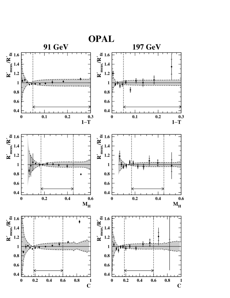
Figure 19: Fits of $\alpha_{\mathrm{s}}$ to event shape distributions for $1-T$, $M_{\mathrm{H}}$ and $C$ at 91 GeV and 197 GeV (i.e. combined 189–209 GeV). Each data point shows the measured bin contents divided by the integral of the predicted distribution across the bin; the inner error bars indicate statistical uncertainties, and the outer bars show the combined statistical and experimental contributions. The dashed curves represent fractional variations in the predicted distributions, corresponding to our perturbative theory uncertainties in $\alpha_{\mathrm{s}}$. The slightly wider shaded bands indicate the combined theory and hadronization uncertainties. The ranges used for fitting each distribution are shown by horizontal arrows.

The fit results are summarized in Table 9 for the four c.m. energy points presented previously. In addition, further fit results are presented in Table 10 for various other groupings of the data in c.m. energy. The statistical error on the fitted value of $\alpha_{\mathrm{s}}$ was estimated from the variation of $\chi^{2}$ by $\pm 1$ about its minimum. Systematic uncertainties were assessed using the techniques described in Sect. 5.3. For each variant of the analysis, the corresponding distribution was fitted to determine $\alpha_{\mathrm{s}}$, and the difference with respect to the value of $\alpha_{\mathrm{s}}$ from the default analysis was taken as a systematic error contribution. In Figs. 19 and 20 we show the ratio of the data to the fitted theory for each of the six event shapes at 91 GeV and 197 GeV respectively. Because of normalization, the theory predictions are seen to “pivot” about some value of $y$, which indicates that the data at that point have no sensitivity to $\alpha_{\mathrm{s}}$.

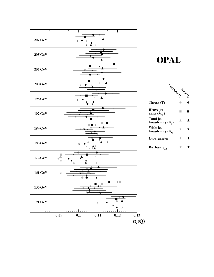
Figure 21: Measurements of $\alpha_{\mathrm{s}}$ using fits to distributions of six event shape observables. The inner error bars represent statistical uncertainties and the outer error bars the total uncertainties. The grey symbols indicate, without errors, previously published OPAL measurements, which are superseded by our new results.

The measurements of $\alpha_{\mathrm{s}}$ for each observable and c.m. energy are shown in Figure 21. We note that the values of $\alpha_{\mathrm{s}}$ at 91 GeV are significantly higher than at LEP II energies, providing evidence for the running of $\alpha_{\mathrm{s}}$. Systematic differences between the values of $\alpha_{\mathrm{s}}$ obtained from different observables are seen; for example, $(1-T)$ and $B_{\mathrm{T}}$ tend to give higher than average values of $\alpha_{\mathrm{s}}$, whilst $B_{\mathrm{W}}$ tends to give the lowest value. These differences may be ascribed to the differing effects of uncomputed higher order terms on the various observables; they are often greater than the statistical errors, but are covered by the systematic uncertainties. There are also significant statistical correlations between the values of $\alpha_{\mathrm{s}}$ obtained from the different observables at a given energy, so that the scatter of the points at energies where the statistics are low (e.g. 161 GeV) tends to be smaller than one would expect if the statistical errors were uncorrelated.

It is useful to combine the measurements of $\alpha_{\mathrm{s}}$ from different observables and/or c.m. energy points, in order to exploit the data fully. This problem has been the subject of extensive study within the LEP QCD working group [53], and we adopt their procedure here. In brief, the method is as follows. The $\alpha_{\mathrm{s}}$ measurements to be combined are first evolved to a common scale, $Q=M_{\mathrm{Z}}$, assuming the validity of QCD. Their combination is then performed using a weighted mean method, such as to minimize the $\chi^{2}$ between the combined value and the measurements. So, if the measured values evolved to $Q=M_{\mathrm{Z}}$ are denoted $\alpha_{i}$ with covariance matrix $V$, the combined value, $\alpha_{\mathrm{s}}(M_{\mathrm{Z}})$, is given by

$$\alpha_{\mathrm{s}}(M_{\mathrm{Z}})=\sum_{i}w_{i}\alpha_{i}\;\;\;\;\;\mathrm{where}\;\;\;\;\;w_{i}=\sum_{j}(V^{-1})_{ij}/\sum_{j,k}(V^{-1})_{jk}\;.$$ (21)

The combined values may then be evolved back to the original scale if required. The difficulty resides in making a reliable estimate of $V$ in the presence of dominant and highly correlated systematic errors; small uncertainties in the estimation of these correlations can easily cause undesirable features such as negative weights. For this reason, only statistical errors (estimated using data-sized subsamples of Monte Carlo events to assess correlations between different observables in a given data sample) and experimental systematic errors (for which the correlations are estimated using the “minimum overlap” assumption) were allowed to contribute to the off-diagonal elements in $V$ when computing the weights, while all error contributions were included in the diagonal terms. The hadronization and theoretical uncertainties were computed by combining the $\alpha_{\mathrm{s}}$ values obtained with the alternative hadronization models, and from the upper and lower theoretical errors, using the same weights.

If the full covariance matrix were used to compute the weights $w_{i}$, then this choice of weights would have the effect of minimising the total error. However, the correlations between the systematic errors cannot be completely reliably estimated (as manifested by the occurrence of negative weights). The modified procedure adopted here will not in general minimize the error, and indeed the error on the weighted average may be greater than one of the inputs; this actually arises in our data for the case of $y^{\mathrm{D}}_{23}$. Despite this, we consider the combined value to provide the safest estimate of $\alpha_{\mathrm{s}}$, since it cannot be guaranteed that the relatively small theoretical error for $y^{\mathrm{D}}_{23}$ is not fortuitous.

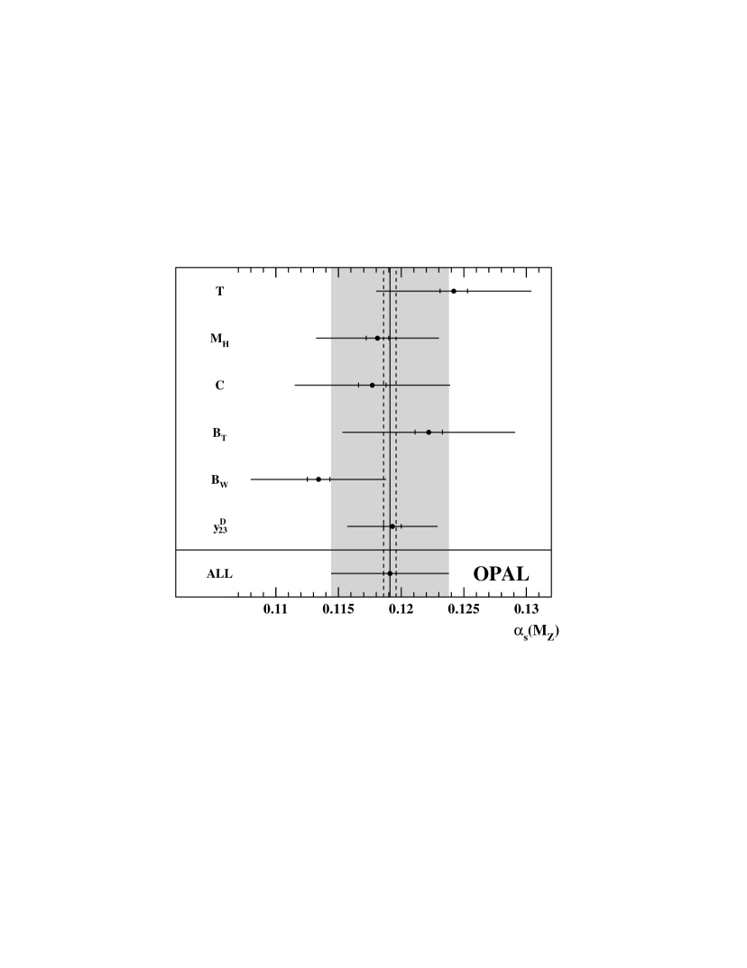
Figure 22: OPAL combinations of $\alpha_{\mathrm{s}}(M_{\mathrm{Z}})$ values inferred from distributions of individual event shape observables. The inner error bars are statistical, while the outer bars represent total uncertainties. The grey band corresponds to the total uncertainty of the combined $\alpha_{\mathrm{s}}(M_{\mathrm{Z}})$ value, and the dashed lines indicate its statistical uncertainty.

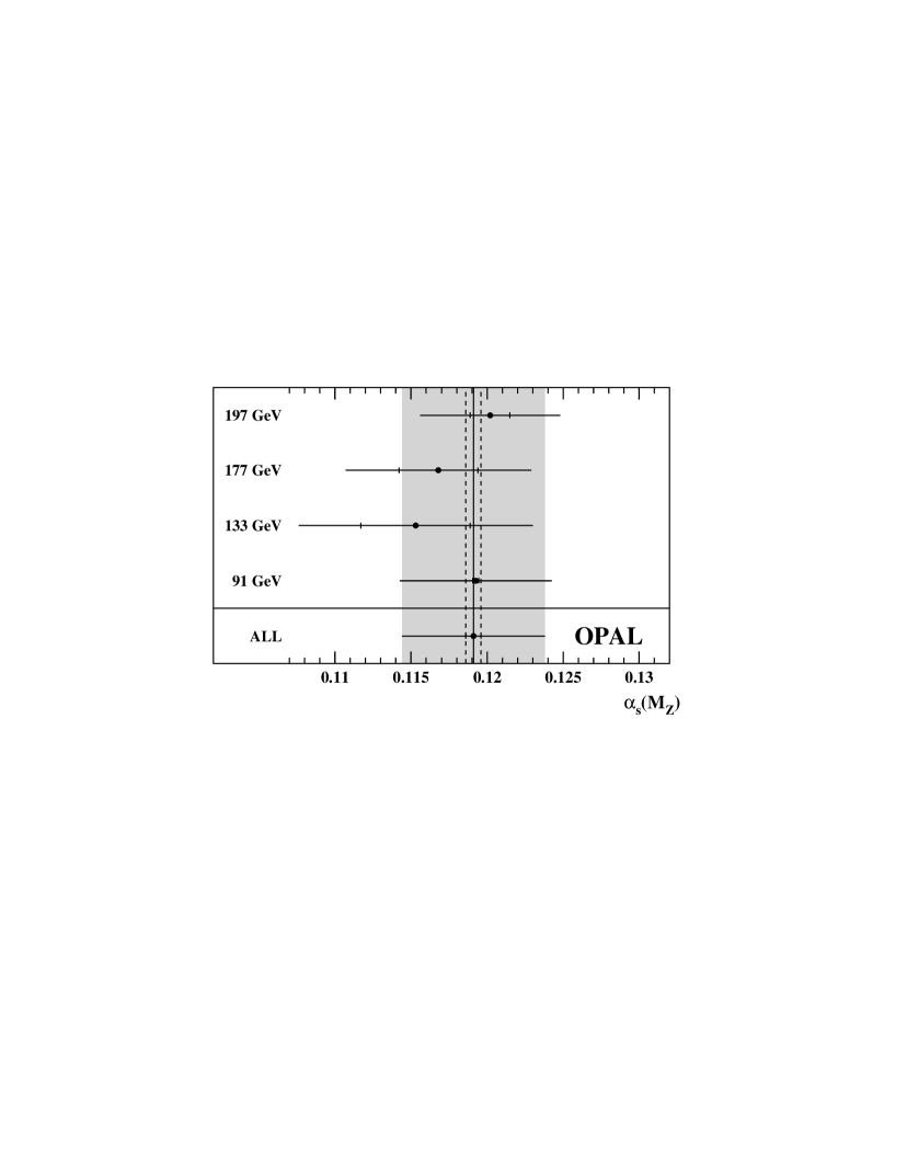
Figure 23: OPAL $\alpha_{\mathrm{s}}(M_{\mathrm{Z}})$ combinations based on distributions of individual event shape observables at different energies. The inner error bars are statistical, while the outer bars represent total uncertainties. The grey band corresponds to the total uncertainty of the combined $\alpha_{\mathrm{s}}(M_{\mathrm{Z}})$ value, and the dashed lines indicate its statistical uncertainty.

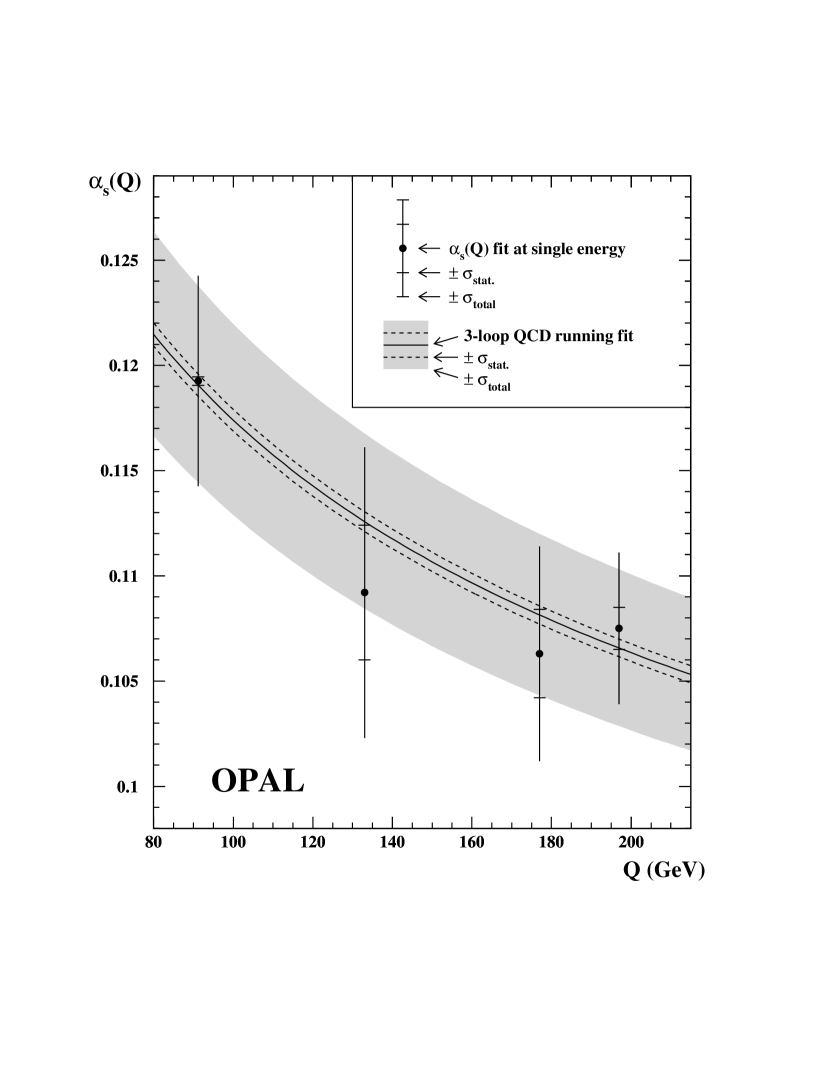
Figure 24: A global QCD running fit to the OPAL $\alpha_{\mathrm{s}}$ measurements based on event shape distributions. Each point represents a fit to the six measurements at an individual centre-of-mass energy, while the curve represents a global fit to all measurements. The form of the curve is determined by the $\mathcal{O}(\alpha_{\mathrm{s}}^{3})$ Renormalization Group Equation of QCD, with $\alpha_{\mathrm{s}}(M_{\mathrm{Z}})$ as a free parameter. The grey band corresponds to the total uncertainty of the fitted $\alpha_{\mathrm{s}}(M_{\mathrm{Z}})$ value, and the dashed curves indicate the statistical uncertainty.

In Table 11 we give the values of $\alpha_{\mathrm{s}}$ for each observable, evolved to a common scale $M_{\mathrm{Z}}$, combined over all c.m. energies. These results are also summarized in Figure 22. This shows clearly that the measurements from the different observables are far from compatible when only statistical errors are considered, but are consistent with a common mean when the systematic errors are included. The results of combining the $\alpha_{\mathrm{s}}$ values for the six observables are given in the rightmost columns of Tables 9 and 10. In addition, the relative weight, $w_{i}$, carried by each observable is given, from which we see that $y^{\mathrm{D}}_{23}$ generally carries the greatest weight (because it has the smallest theoretical uncertainty). These results are plotted in Figure 23 where we show the values at each energy evolved to a common scale, $\alpha_{\mathrm{s}}(M_{\mathrm{Z}})$, and in Figure 24 where we show $\alpha_{\mathrm{s}}$ as a function of the energy scale $Q=E_{\mathrm{c.m.}}$. These plots show that the variation of $\alpha_{\mathrm{s}}$ with $E_{\mathrm{c.m.}}$ is consistent with the running predicted by QCD, and is incompatible with a constant value of $\alpha_{\mathrm{s}}$. For example, the two most precise values of $\alpha_{\mathrm{s}}$, at 91 and 197 GeV, differ by more than three standard deviations (applying the minimum overlap ansatz to the systematic errors).

The measurement of $\alpha_{\mathrm{s}}$ based on the 91 GeV data is

$$\alpha_{\mathrm{s}}(M_{\mathrm{Z}})=0.1192\pm 0.0002~{}\mathrm{(stat.)}\pm 0.0008~{}\mathrm{(expt.)}\pm 0.0015~{}\mathrm{(hadr.)}\pm 0.0047~{}\mathrm{(theo.)}$$

while the result for $\alpha_{\mathrm{s}}(M_{\mathrm{Z}})$ combining all higher energy data at $Q>M_{\mathrm{Z}}$ is

$$\alpha_{\mathrm{s}}(M_{\mathrm{Z}})=0.1189\pm 0.0011~{}\mathrm{(stat.)}\pm 0.0015~{}\mathrm{(expt.)}\pm 0.0008~{}\mathrm{(hadr.)}\pm 0.0040~{}\mathrm{(theo.)}\;.$$

The consistency between these measurements, which are equal within the statistical errors, again shows that the data are compatible with the running predicted by QCD, since this running was assumed in evolving the high energy data to $Q=M_{\mathrm{Z}}$. We note that the high energy data have significantly smaller theoretical and hadronization errors, and therefore complement the statistically superior 91 GeV data. The value of $\alpha_{\mathrm{s}}(M_{\mathrm{Z}})$ obtained from all observables and all energies combined is:

$$\framebox{$\begin{array}[]{rcl}\alpha_{\mathrm{s}}(M_{\mathrm{Z}})&=&0.1191\pm 0.0005~{}\mathrm{(stat.)}\pm 0.0010~{}\mathrm{(expt.)}\pm 0.0011~{}\mathrm{(hadr.)}\pm 0.0044~{}\mathrm{(theo.)}\\ &=&0.1191\pm 0.0005~{}\mathrm{(stat.)}\pm 0.0046~{}\mathrm{(syst.)}\\ &=&0.1191\pm 0.0047~{}\mathrm{(total)}\end{array}$}$$

6.3.2 Determination of $\alpha_{\mathrm{s}}$ using event shape moments

The strong coupling $\alpha_{\mathrm{s}}(M_{\mathrm{Z}})$ has also been determined from the measured moments using the $\mathcal{O}(\alpha_{\mathrm{s}}^{2})$ QCD predictions explained in Sect. 4.3. This is the first such study to be published by the OPAL Collaboration. The first five moments of the observables $1-T$, $M_{\mathrm{H}}$, $B_{\mathrm{T}}$, $B_{\mathrm{W}}$, $C$ and $y^{\mathrm{D}}_{23}$ were studied, i.e. the same observables as used for the determination of $\alpha_{\mathrm{s}}$ from distributions. One might anticipate a priori that this would yield a less precise determination of $\alpha_{\mathrm{s}}$ than the differential distributions, because the theory lacks resummation of large logarithms, and the moments include regions of phase space where hadronization effects are large. Nevertheless, the comparison of $\alpha_{\mathrm{s}}$ determined in this way with that obtained from the distributions should provide an illuminating test of the adequacy of QCD in this area.

The fits proceeded by comparing the data at the four combined energy points for a given moment of an observable with the theory prediction. The running of $\alpha_{\mathrm{s}}$ was implemented in the fit in two-loop precision using the formula given in ref. [54]. A value of $\chi^{2}$ was calculated using the statistical errors of the data and minimized to extract a value of $\alpha_{\mathrm{s}}(M_{\mathrm{Z}})$. The fits were repeated for each systematic variation of the analysis. The statistical error was found as above by variation of $\chi^{2}$ by $\pm 1$ about the minimum.

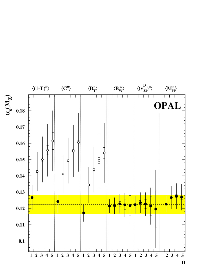
Figure 25: Measurements of $\alpha_{\mathrm{s}}$ using fits to moments of six event shape observables. The inner error bars represent statistical uncertainties, and the outer error bars show the total errors. The dashed line indicates the weighted average described in the text; only the measurements indicated by solid symbols were used for this purpose.

The fit results are shown in Table 12 and in Figure 25. The fit to $\langle M_{\mathrm{H}}\rangle$ was not stable and therefore no results are shown. We obtain values of $\chi^{2}/\mathrm{d.o.f.}$ of $\mathcal{O}(1)$; the fitted QCD predictions including the running of $\alpha_{\mathrm{s}}$ are thus consistent with our data. However, we find that for $\langle(1-T)^{n}\rangle$, $\langle C^{n}\rangle$ and $\langle B_{\mathrm{T}}^{n}\rangle$ the fitted values of $\alpha_{\mathrm{s}}(M_{\mathrm{Z}})$ increase with the order $n$ of the moment used. This effect is not observed for $\langle B_{\mathrm{W}}^{n}\rangle$, $\langle(y^{\mathrm{D}}_{23})^{n}\rangle$ and $\langle M_{\mathrm{H}}^{n}\rangle$, $n=2,\ldots,5$. In order to investigate the origin of this behaviour we show in Figure 26 the ratio $K={\cal B}_{n}/{\cal A}_{n}$ of NLO and LO coefficients for the six observables used in our fits. There is a clear correlation between the increasing values of $\alpha_{\mathrm{s}}(M_{\mathrm{Z}})$ with moment $n$ and increasing values of $K$ with $n$ for $\langle(1-T)^{n}\rangle$, $\langle C^{n}\rangle$ and $\langle B_{\mathrm{T}}^{n}\rangle$. The other observables $\langle B_{\mathrm{W}}^{n}\rangle$, $\langle(y^{\mathrm{D}}_{23})^{n}\rangle$ and $\langle M_{\mathrm{H}}^{n}\rangle$, $n=2,\ldots,5$, have fairly constant values of $K$ and correspondingly stable results for $\alpha_{\mathrm{s}}(M_{\mathrm{Z}})$. We also note that $\langle M_{\mathrm{H}}\rangle$ has a large and negative value of $K$ which is the cause of the unstable fits.

In order to combine the individual determinations of $\alpha_{\mathrm{s}}(M_{\mathrm{Z}})$ we used the same weighted average method as in Sect. 6.3.1. We considered only those results for which the fit was successful and for which the NLO term in equation (17) is less than half the LO term (i.e.  $|K\alpha_{\mathrm{s}}/2\pi|<0.5$ or $|K|\lesssim 25$), namely $\langle 1-T\rangle$, $\langle C\rangle$, $\langle B_{\mathrm{T}}\rangle$, $\langle B_{\mathrm{W}}^{n}\rangle$ and $\langle(y^{\mathrm{D}}_{23})^{n}\rangle$, $n=1,\ldots,5$ and $\langle M_{\mathrm{H}}^{n}\rangle$, $n=2,\ldots,5$; i.e. results from 17 observables in total. The statistical correlations between the 17 results were determined using Monte Carlo simulation at the hadron-level. The experimental errors were included in the covariance matrix using the minimum-overlap assumption while the hadronization and renormalization scale uncertainties were only added to the diagonal of the covariance matrix. The combination was repeated using the same weights with the HERWIG and ARIADNE hadronization corrections and for $x_{\mu}=0.5$ and $x_{\mu}=2.0$ for the calculation of the hadronization theory systematic errors. The weights were generally $\mathcal{O}(10\%)$ for each observable; the largest weight was 23% for $\langle B_{\mathrm{T}}\rangle$ while the only weights below 3% were those for $\langle(y^{\mathrm{D}}_{23})^{5}\rangle$ $\langle M_{\mathrm{H}}^{3}\rangle$ and $\langle M_{\mathrm{H}}^{4}\rangle$. The result is

$$\begin{array}[]{rcl}\alpha_{\mathrm{s}}(M_{\mathrm{Z}})&=&0.1223\pm 0.0005~{}\mathrm{(stat.)}\pm 0.0014~{}\mathrm{(expt.)}\pm 0.0016~{}\mathrm{(hadr.)}^{+0.0054}_{-0.0036}\mathrm{(theo.)}\\ &=&0.1223\pm 0.0005~{}\mathrm{(stat.)}\pm 0.0058~{}\mathrm{(syst.)}\\ &=&0.1223\pm 0.0059~{}\mathrm{(total)}\end{array}$$

in good agreement with the result from distributions presented in Sect. 6.3.1.

The experimental, hadronization and theory uncertainties are somewhat larger than for the distributions. In an analysis using moments the complete available phase space is sampled including regions which are more difficult to measure experimentally and which are less reliably modelled by the hadronization models. Also, the NLO QCD prediction is less complete than the matched $\mathcal{O}(\alpha_{\mathrm{s}}^{2})$+NLLA prediction available for the distributions which we studied. It is nevertheless a remarkable success of QCD together with the corresponding hadronization models that the NLO theory is able to describe successfully some observables based on the complete available phase space.

7 Summary and conclusions

In this paper we have presented measurements of the event shapes for hadronic events produced at LEP at centre-of-mass energies between 91 and 209 GeV. Both differential distributions and moments have been determined.

The predictions of the PYTHIA, HERWIG and ARIADNE Monte Carlo models are found to be in general agreement with the measured distributions and moments. However, some discrepancies are noted in the 91 GeV data where the statistical errors are smallest. The main differences between models and data occur in the extreme two-jet region, and for observables sensitive to the production of four or more jets. In general, ARIADNE provides the best description of the data and HERWIG the least good.

From a fit of $\mathcal{O}(\alpha_{\mathrm{s}}^{2})$+NLLA QCD predictions to the distributions of six event shape observables, we have determined the strong coupling parameter $\alpha_{\mathrm{s}}$. The variation of $\alpha_{\mathrm{s}}$ with energy scale over the range 91 to 209 GeV is found to be in accordance with the expectations of QCD. For example, the measurement of $\alpha_{\mathrm{s}}$ based on the 91 GeV data is

$$\alpha_{\mathrm{s}}(M_{\mathrm{Z}})=0.1192\pm 0.0002~{}\mathrm{(stat.)}\pm 0.0008~{}\mathrm{(expt.)}\pm 0.0015~{}\mathrm{(hadr.)}\pm 0.0047~{}\mathrm{(theo.)}\;.$$

Assuming the validity of QCD, the higher energy measurements can all be evolved to a common scale $Q=M_{\mathrm{Z}}$ and combined, yielding the following result for $\alpha_{\mathrm{s}}(M_{\mathrm{Z}})$ combining all higher energy data at $Q>M_{\mathrm{Z}}$

$$\alpha_{\mathrm{s}}(M_{\mathrm{Z}})=0.1189\pm 0.0011~{}\mathrm{(stat.)}\pm 0.0015~{}\mathrm{(expt.)}\pm 0.0008~{}\mathrm{(hadr.)}\pm 0.0040~{}\mathrm{(theo.)}\;.$$

Combining all data at all energy scales, the value of $\alpha_{\mathrm{s}}(M_{\mathrm{Z}})$ is determined to be

$$\alpha_{\mathrm{s}}(M_{\mathrm{Z}})=0.1191\pm 0.0005~{}\mathrm{(stat.)}\pm 0.0010~{}\mathrm{(expt.)}\pm 0.0011~{}\mathrm{(hadr.)}\pm 0.0044~{}\mathrm{(theo.)}\;,$$

in good agreement with the world average quoted in ref. [54]. The results for $\alpha_{\mathrm{s}}(M_{\mathrm{Z}})$ derived from different event shapes are consistent within errors.

Values of $\alpha_{\mathrm{s}}(M_{\mathrm{Z}})$ have also been derived from the energy dependence of event shape moments, using $\mathcal{O}(\alpha_{\mathrm{s}}^{2})$ QCD. Although less complete than the $\mathcal{O}(\alpha_{\mathrm{s}}^{2})$+NLLA QCD predictions used for the distributions, these calculations prove to give a consistent description of many, though not all, of the moments. The combined value obtained from the moments was $\alpha_{\mathrm{s}}(M_{\mathrm{Z}})=0.1223\pm 0.0005~{}\mathrm{(stat.)}\pm 0.0014~{}\mathrm{(expt.)}\pm 0.0016~{}\mathrm{(hadr.)}^{+0.0054}_{-0.0036}\mathrm{(theo.)}\;,$ consistent with that derived from the distributions. However, because the value obtained from the distributions is based on the more complete theory (and has a smaller overall error) we consider that to be the most reliable estimate from the present data.

Year	Range of $\sqrt{s}$ (GeV)		Mean $\sqrt{s}$ (GeV)	Integrated luminosity (pb-1)	Number of selected events	Expected number
1996–2000	91.0 –	91.5	91.3	14.7	395695	—
1995, 1997	129.9 –	136.3	133.1	11.26	630	698
1996	161.2 –	161.6	161.3	10.06	281	275
1996	170.2 –	172.5	172.1	10.38	218	232
1997	180.8 –	184.2	182.7	57.72	1077	1084
1998	188.3 –	189.1	188.6	185.2	3086	3130
1999	191.4 –	192.1	191.6	29.53	514	473
1999	195.4 –	196.1	195.5	76.67	1137	1161
1999, 2000	199.1 –	200.2	199.5	79.27	1090	1131
1999, 2000	201.3 –	202.1	201.6	37.75	519	527
2000	202.5 –	205.5	204.9	82.01	1130	1090
2000	205.5 –	208.9	206.6	138.8	1717	1804

Table 1: The OPAL data samples used for the present analysis. The horizontal lines separate the data into the four energy ranges used for presentation purposes.

$1-T$		$R^{\prime}\,(1-T)$ at 91 GeV							$R^{\prime}\,(1-T)$ at 133 GeV							$R^{\prime}\,(1-T)$ at 177 GeV							$R^{\prime}\,(1-T)$ at 197 GeV
[t] $0.00$ –	$0.01$	1.	276 $\pm$	0.	019 $\pm$	0.	040		4.	37 $\pm$	0.	82 $\pm$	0.	55		8.	76 $\pm$	0.	74 $\pm$	0.	64		9.	95 $\pm$	0.	34 $\pm$	0.	27
$0.01$ –	$0.02$	12.	25 $\pm$	0.	05 $\pm$	0.	41		20.	4 $\pm$	1.	6 $\pm$	3.	8		22.	65 $\pm$	1.	11 $\pm$	1.	23		22.	44 $\pm$	0.	47 $\pm$	0.	40
$0.02$ –	$0.03$	18.	38 $\pm$	0.	06 $\pm$	0.	27		20.	4 $\pm$	1.	5 $\pm$	1.	7		16.	25 $\pm$	0.	92 $\pm$	0.	76		14.	92 $\pm$	0.	37 $\pm$	0.	56
$0.03$ –	$0.04$	13.	87 $\pm$	0.	06 $\pm$	0.	14		10.	5 $\pm$	1.	2 $\pm$	0.	9		9.	84 $\pm$	0.	73 $\pm$	0.	98		9.	57 $\pm$	0.	31 $\pm$	0.	41
$0.04$ –	$0.05$	9.	83 $\pm$	0.	05 $\pm$	0.	16		6.	7 $\pm$	1.	0 $\pm$	0.	4		6.	85 $\pm$	0.	65 $\pm$	0.	87		7.	23 $\pm$	0.	27 $\pm$	0.	20
$0.05$ –	$0.07$	6.	502 $\pm$	0.	026 $\pm$	0.	088		4.	70 $\pm$	0.	58 $\pm$	0.	35		4.	96 $\pm$	0.	38 $\pm$	0.	20		5.	24 $\pm$	0.	16 $\pm$	0.	15
$0.07$ –	$0.09$	4.	127 $\pm$	0.	022 $\pm$	0.	041		3.	64 $\pm$	0.	51 $\pm$	0.	29		3.	18 $\pm$	0.	33 $\pm$	0.	27		2.	87 $\pm$	0.	14 $\pm$	0.	15
$0.09$ –	$0.12$	2.	646 $\pm$	0.	014 $\pm$	0.	058		1.	68 $\pm$	0.	32 $\pm$	0.	44		2.	05 $\pm$	0.	23 $\pm$	0.	19		2.	28 $\pm$	0.	09 $\pm$	0.	07
$0.12$ –	$0.15$	1.	709 $\pm$	0.	012 $\pm$	0.	079		1.	36 $\pm$	0.	24 $\pm$	0.	32		1.	28 $\pm$	0.	19 $\pm$	0.	21		1.	40 $\pm$	0.	08 $\pm$	0.	10
$0.15$ –	$0.22$	0.	910 $\pm$	0.	005 $\pm$	0.	019		1.	09 $\pm$	0.	12 $\pm$	0.	18		0.	82 $\pm$	0.	10 $\pm$	0.	10		0.	787 $\pm$	0.	047 $\pm$	0.	057
$0.22$ –	$0.30$	0.	3705 $\pm$	0.	0032 $\pm$	0.	0092		0.	467 $\pm$	0.	065 $\pm$	0.	066		0.	342 $\pm$	0.	075 $\pm$	0.	088		0.	382 $\pm$	0.	046 $\pm$	0.	065	[b]
$M_{\mathrm{H}}$		$R^{\prime}\,(M_{\mathrm{H}})$ at 91 GeV							$R^{\prime}\,(M_{\mathrm{H}})$ at 133 GeV							$R^{\prime}\,(M_{\mathrm{H}})$ at 177 GeV							$R^{\prime}\,(M_{\mathrm{H}})$ at 197 GeV
[t] $0.060$ –	$0.075$	0.	119 $\pm$	0.	003 $\pm$	0.	010		0.	38 $\pm$	0.	16 $\pm$	0.	13		1.	35 $\pm$	0.	18 $\pm$	0.	44		1.	93 $\pm$	0.	09 $\pm$	0.	17
$0.075$ –	$0.090$	0.	55 $\pm$	0.	01 $\pm$	0.	13		1.	56 $\pm$	0.	35 $\pm$	0.	36		4.	33 $\pm$	0.	36 $\pm$	0.	58		4.	62 $\pm$	0.	17 $\pm$	0.	19
$0.090$ –	$0.110$	2.	16 $\pm$	0.	01 $\pm$	0.	39		4.	69 $\pm$	0.	53 $\pm$	1.	25		6.	21 $\pm$	0.	45 $\pm$	0.	59		6.	55 $\pm$	0.	19 $\pm$	0.	23
$0.110$ –	$0.140$	5.	72 $\pm$	0.	02 $\pm$	0.	05		8.	18 $\pm$	0.	54 $\pm$	1.	05		6.	06 $\pm$	0.	34 $\pm$	0.	43		5.	82 $\pm$	0.	14 $\pm$	0.	30
$0.140$ –	$0.170$	6.	66 $\pm$	0.	02 $\pm$	0.	36		4.	99 $\pm$	0.	48 $\pm$	0.	82		5.	06 $\pm$	0.	30 $\pm$	0.	26		4.	66 $\pm$	0.	12 $\pm$	0.	16
$0.170$ –	$0.200$	4.	88 $\pm$	0.	02 $\pm$	0.	15		3.	92 $\pm$	0.	43 $\pm$	0.	28		3.	47 $\pm$	0.	26 $\pm$	0.	43		3.	53 $\pm$	0.	11 $\pm$	0.	16
$0.200$ –	$0.250$	3.	29 $\pm$	0.	01 $\pm$	0.	12		2.	47 $\pm$	0.	27 $\pm$	0.	30		2.	54 $\pm$	0.	18 $\pm$	0.	36		2.	37 $\pm$	0.	07 $\pm$	0.	12
$0.250$ –	$0.300$	2.	107 $\pm$	0.	010 $\pm$	0.	054		1.	41 $\pm$	0.	23 $\pm$	0.	22		1.	54 $\pm$	0.	16 $\pm$	0.	28		1.	60 $\pm$	0.	07 $\pm$	0.	09
$0.300$ –	$0.350$	1.	352 $\pm$	0.	008 $\pm$	0.	042		1.	35 $\pm$	0.	18 $\pm$	0.	23		1.	25 $\pm$	0.	14 $\pm$	0.	18		1.	22 $\pm$	0.	06 $\pm$	0.	12
$0.350$ –	$0.450$	0.	703 $\pm$	0.	004 $\pm$	0.	031		0.	758 $\pm$	0.	088 $\pm$	0.	075		0.	647 $\pm$	0.	079 $\pm$	0.	085		0.	641 $\pm$	0.	035 $\pm$	0.	031
$0.450$ –	$0.600$	0.	1372 $\pm$	0.	0016 $\pm$	0.	0036		0.	162 $\pm$	0.	033 $\pm$	0.	016		0.	114 $\pm$	0.	032 $\pm$	0.	042		0.	149 $\pm$	0.	019 $\pm$	0.	039	[b]
$C$		$R^{\prime}\,(C)$ at 91 GeV							$R^{\prime}\,(C)$ at 133 GeV							$R^{\prime}\,(C)$ at 177 GeV							$R^{\prime}\,(C)$ at 197 GeV
[t] $0.00$ –	$0.05$	0.	2186 $\pm$	0.	0038 $\pm$	0.	0060		0.	83 $\pm$	0.	17 $\pm$	0.	11		1.	97 $\pm$	0.	16 $\pm$	0.	12		2.	079 $\pm$	0.	071 $\pm$	0.	053
$0.05$ –	$0.08$	2.	061 $\pm$	0.	013 $\pm$	0.	108		4.	07 $\pm$	0.	45 $\pm$	1.	17		5.	04 $\pm$	0.	32 $\pm$	0.	31		5.	225 $\pm$	0.	136 $\pm$	0.	159
$0.08$ –	$0.11$	4.	037 $\pm$	0.	018 $\pm$	0.	052		5.	70 $\pm$	0.	46 $\pm$	0.	51		4.	32 $\pm$	0.	28 $\pm$	0.	43		3.	797 $\pm$	0.	113 $\pm$	0.	235
$0.11$ –	$0.14$	4.	152 $\pm$	0.	018 $\pm$	0.	047		3.	86 $\pm$	0.	39 $\pm$	0.	41		3.	26 $\pm$	0.	24 $\pm$	0.	14		3.	076 $\pm$	0.	099 $\pm$	0.	052
$0.14$ –	$0.18$	3.	225 $\pm$	0.	013 $\pm$	0.	044		2.	55 $\pm$	0.	29 $\pm$	0.	14		2.	30 $\pm$	0.	18 $\pm$	0.	22		2.	382 $\pm$	0.	075 $\pm$	0.	045
$0.18$ –	$0.22$	2.	421 $\pm$	0.	012 $\pm$	0.	060		1.	65 $\pm$	0.	25 $\pm$	0.	19		1.	73 $\pm$	0.	16 $\pm$	0.	11		1.	757 $\pm$	0.	067 $\pm$	0.	026
$0.22$ –	$0.30$	1.	705 $\pm$	0.	007 $\pm$	0.	020		1.	22 $\pm$	0.	15 $\pm$	0.	07		1.	317 $\pm$	0.	097 $\pm$	0.	085		1.	330 $\pm$	0.	041 $\pm$	0.	033
$0.30$ –	$0.40$	1.	112 $\pm$	0.	005 $\pm$	0.	012		0.	93 $\pm$	0.	11 $\pm$	0.	06		0.	853 $\pm$	0.	076 $\pm$	0.	067		0.	850 $\pm$	0.	032 $\pm$	0.	028
$0.40$ –	$0.50$	0.	747 $\pm$	0.	004 $\pm$	0.	017		0.	43 $\pm$	0.	09 $\pm$	0.	12		0.	573 $\pm$	0.	067 $\pm$	0.	062		0.	623 $\pm$	0.	028 $\pm$	0.	017
$0.50$ –	$0.60$	0.	535 $\pm$	0.	004 $\pm$	0.	024		0.	73 $\pm$	0.	08 $\pm$	0.	15		0.	488 $\pm$	0.	063 $\pm$	0.	072		0.	453 $\pm$	0.	027 $\pm$	0.	026
$0.60$ –	$0.75$	0.	3693 $\pm$	0.	0024 $\pm$	0.	0082		0.	334 $\pm$	0.	051 $\pm$	0.	061		0.	318 $\pm$	0.	048 $\pm$	0.	055		0.	341 $\pm$	0.	025 $\pm$	0.	047
$0.75$ –	$1.00$	0.	0982 $\pm$	0.	0009 $\pm$	0.	0023		0.	101 $\pm$	0.	018 $\pm$	0.	021		0.	069 $\pm$	0.	029 $\pm$	0.	034		0.	070 $\pm$	0.	021 $\pm$	0.	045	[b]

Table 2: Distributions for the thrust $(1-T)$, heavy jet mass ($M_{\mathrm{H}}$) and $C$-parameter measured by OPAL at centre-of-mass energies $\sqrt{s}=91$, 130–136, 161–183, and 189–209 GeV. The first uncertainty is statistical, while the second is systematic.

$B_{\mathrm{T}}$		$R^{\prime}\,(B_{\mathrm{T}})$ at 91 GeV							$R^{\prime}\,(B_{\mathrm{T}})$ at 133 GeV							$R^{\prime}\,(B_{\mathrm{T}})$ at 177 GeV							$R^{\prime}\,(B_{\mathrm{T}})$ at 197 GeV
[t] $0.000$ –	$0.030$	0.	117 $\pm$	0.	005 $\pm$	0.	012		0.	58 $\pm$	0.	26 $\pm$	0.	16		1.	78 $\pm$	0.	23 $\pm$	0.	18		2.	40 $\pm$	0.	12 $\pm$	0.	07
$0.030$ –	$0.040$	2.	50 $\pm$	0.	03 $\pm$	0.	11		10.	2 $\pm$	1.	1 $\pm$	1.	3		12.	1 $\pm$	0.	9 $\pm$	1.	2		11.	23 $\pm$	0.	41 $\pm$	0.	44
$0.040$ –	$0.050$	6.	95 $\pm$	0.	04 $\pm$	0.	13		9.	6 $\pm$	1.	3 $\pm$	1.	9		11.	5 $\pm$	0.	8 $\pm$	1.	2		10.	99 $\pm$	0.	38 $\pm$	0.	49
$0.050$ –	$0.060$	9.	806 $\pm$	0.	050 $\pm$	0.	079		11.	9 $\pm$	1.	2 $\pm$	0.	9		11.	01 $\pm$	0.	75 $\pm$	0.	79		9.	67 $\pm$	0.	34 $\pm$	0.	56
$0.060$ –	$0.075$	10.	744 $\pm$	0.	040 $\pm$	0.	120		10.	06 $\pm$	0.	86 $\pm$	0.	52		8.	29 $\pm$	0.	55 $\pm$	0.	43		7.	74 $\pm$	0.	25 $\pm$	0.	23
$0.075$ –	$0.090$	8.	777 $\pm$	0.	035 $\pm$	0.	211		6.	31 $\pm$	0.	76 $\pm$	0.	36		5.	71 $\pm$	0.	48 $\pm$	0.	36		6.	14 $\pm$	0.	22 $\pm$	0.	35
$0.090$ –	$0.110$	6.	597 $\pm$	0.	026 $\pm$	0.	065		4.	35 $\pm$	0.	59 $\pm$	0.	82		4.	38 $\pm$	0.	37 $\pm$	0.	38		4.	85 $\pm$	0.	18 $\pm$	0.	16
$0.110$ –	$0.130$	4.	829 $\pm$	0.	023 $\pm$	0.	074		4.	36 $\pm$	0.	52 $\pm$	0.	41		3.	64 $\pm$	0.	34 $\pm$	0.	36		3.	43 $\pm$	0.	15 $\pm$	0.	14
$0.130$ –	$0.160$	3.	386 $\pm$	0.	016 $\pm$	0.	050		2.	43 $\pm$	0.	36 $\pm$	0.	25		2.	78 $\pm$	0.	24 $\pm$	0.	30		2.	60 $\pm$	0.	11 $\pm$	0.	08
$0.160$ –	$0.200$	2.	130 $\pm$	0.	011 $\pm$	0.	047		1.	71 $\pm$	0.	24 $\pm$	0.	22		1.	50 $\pm$	0.	18 $\pm$	0.	17		1.	747 $\pm$	0.	081 $\pm$	0.	063
$0.200$ –	$0.250$	1.	186 $\pm$	0.	007 $\pm$	0.	025		1.	25 $\pm$	0.	16 $\pm$	0.	30		1.	13 $\pm$	0.	15 $\pm$	0.	13		1.	008 $\pm$	0.	069 $\pm$	0.	085
$0.250$ –	$0.300$	0.	565 $\pm$	0.	005 $\pm$	0.	015		0.	72 $\pm$	0.	10 $\pm$	0.	09		0.	42 $\pm$	0.	12 $\pm$	0.	11		0.	443 $\pm$	0.	082 $\pm$	0.	073
$0.300$ –	$0.350$	0.	1557 $\pm$	0.	0024 $\pm$	0.	0049		0.	128 $\pm$	0.	042 $\pm$	0.	059		0.	05 $\pm$	0.	09 $\pm$	0.	13		0.	096 $\pm$	0.	082 $\pm$	0.	114	[b]
$B_{\mathrm{W}}$		$R^{\prime}\,(B_{\mathrm{W}})$ at 91 GeV							$R^{\prime}\,(B_{\mathrm{W}})$ at 133 GeV							$R^{\prime}\,(B_{\mathrm{W}})$ at 177 GeV							$R^{\prime}\,(B_{\mathrm{W}})$ at 197 GeV
[t] $0.000$ –	$0.020$	0.	557 $\pm$	0.	011 $\pm$	0.	021		3.	15 $\pm$	0.	53 $\pm$	0.	83		5.	29 $\pm$	0.	45 $\pm$	0.	23		5.	93 $\pm$	0.	19 $\pm$	0.	19
$0.020$ –	$0.030$	10.	38 $\pm$	0.	05 $\pm$	0.	15		16.	4 $\pm$	1.	5 $\pm$	2.	5		16.	76 $\pm$	0.	94 $\pm$	1.	33		15.	82 $\pm$	0.	38 $\pm$	0.	90
$0.030$ –	$0.040$	16.	54 $\pm$	0.	06 $\pm$	0.	11		14.	6 $\pm$	1.	3 $\pm$	0.	6		13.	23 $\pm$	0.	83 $\pm$	0.	74		12.	71 $\pm$	0.	34 $\pm$	0.	26
$0.040$ –	$0.050$	13.	32 $\pm$	0.	05 $\pm$	0.	66		10.	7 $\pm$	1.	1 $\pm$	0.	7		11.	09 $\pm$	0.	75 $\pm$	0.	79		10.	13 $\pm$	0.	31 $\pm$	0.	37
$0.050$ –	$0.065$	9.	82 $\pm$	0.	04 $\pm$	0.	13		9.	47 $\pm$	0.	84 $\pm$	0.	84		7.	70 $\pm$	0.	54 $\pm$	0.	51		7.	79 $\pm$	0.	22 $\pm$	0.	18
$0.065$ –	$0.080$	7.	17 $\pm$	0.	03 $\pm$	0.	15		5.	44 $\pm$	0.	72 $\pm$	0.	40		5.	05 $\pm$	0.	47 $\pm$	0.	21		5.	55 $\pm$	0.	20 $\pm$	0.	17
$0.080$ –	$0.100$	5.	061 $\pm$	0.	023 $\pm$	0.	065		3.	96 $\pm$	0.	54 $\pm$	0.	45		4.	24 $\pm$	0.	37 $\pm$	0.	33		4.	19 $\pm$	0.	16 $\pm$	0.	19
$0.100$ –	$0.150$	2.	845 $\pm$	0.	011 $\pm$	0.	066		2.	44 $\pm$	0.	27 $\pm$	0.	24		2.	47 $\pm$	0.	19 $\pm$	0.	12		2.	442 $\pm$	0.	079 $\pm$	0.	096
$0.150$ –	$0.200$	1.	238 $\pm$	0.	008 $\pm$	0.	042		1.	19 $\pm$	0.	16 $\pm$	0.	25		1.	11 $\pm$	0.	15 $\pm$	0.	15		1.	146 $\pm$	0.	066 $\pm$	0.	062
$0.200$ –	$0.250$	0.	465 $\pm$	0.	005 $\pm$	0.	014		0.	63 $\pm$	0.	11 $\pm$	0.	07		0.	47 $\pm$	0.	11 $\pm$	0.	23		0.	506 $\pm$	0.	057 $\pm$	0.	087
$0.250$ –	$0.300$	0.	0625 $\pm$	0.	0017 $\pm$	0.	0029		0.	077 $\pm$	0.	033 $\pm$	0.	057		0.	10 $\pm$	0.	05 $\pm$	0.	10		0.	123 $\pm$	0.	031 $\pm$	0.	095	[b]
$y_{23}^{\mathrm{D}}$		$R^{\prime}\,(y_{23}^{\mathrm{D}})$ at 91 GeV							$R^{\prime}\,(y_{23}^{\mathrm{D}})$ at 133 GeV							$R^{\prime}\,(y_{23}^{\mathrm{D}})$ at 177 GeV							$R^{\prime}\,(y_{23}^{\mathrm{D}})$ at 197 GeV
[t] $0.00030$ –	$0.00075$	146.	5 $\pm$	1.	0 $\pm$	2.	6		299	$\pm$	30	$\pm$	41			323	$\pm$	20	$\pm$	19			334	$\pm$	8	$\pm$	17
$0.00075$ –	$0.00130$	183.	1 $\pm$	0.	9 $\pm$	5.	5		201	$\pm$	22	$\pm$	21			223	$\pm$	14	$\pm$	36			168.	6 $\pm$	5.	5 $\pm$	5.	2
$0.00130$ –	$0.00230$	141.	4 $\pm$	0.	6 $\pm$	3.	1		116	$\pm$	12	$\pm$	22			93	$\pm$	7	$\pm$	16			101.	5 $\pm$	3.	0 $\pm$	4.	8
$0.00230$ –	$0.00400$	81.	8 $\pm$	0.	3 $\pm$	1.	3		62.	6 $\pm$	6.	7 $\pm$	8.	4		53.	1 $\pm$	4.	2 $\pm$	7.	1		58.	9 $\pm$	1.	8 $\pm$	2.	6
$0.00400$ –	$0.00700$	39.	6 $\pm$	0.	2 $\pm$	1.	2		33.	0 $\pm$	3.	9 $\pm$	5.	1		32.	8 $\pm$	2.	6 $\pm$	5.	1		30.	2 $\pm$	1.	0 $\pm$	0.	7
$0.00700$ –	$0.01200$	19.	90 $\pm$	0.	09 $\pm$	0.	22		19.	9 $\pm$	2.	2 $\pm$	3.	1		16.	7 $\pm$	1.	5 $\pm$	1.	4		17.	59 $\pm$	0.	62 $\pm$	0.	30
$0.01200$ –	$0.02250$	9.	73 $\pm$	0.	05 $\pm$	0.	20		6.	9 $\pm$	1.	1 $\pm$	0.	4		8.	67 $\pm$	0.	76 $\pm$	0.	92		8.	96 $\pm$	0.	32 $\pm$	0.	44
$0.02250$ –	$0.04000$	4.	56 $\pm$	0.	02 $\pm$	0.	20		3.	72 $\pm$	0.	60 $\pm$	0.	50		4.	54 $\pm$	0.	41 $\pm$	0.	34		3.	90 $\pm$	0.	18 $\pm$	0.	28
$0.04000$ –	$0.07000$	2.	105 $\pm$	0.	013 $\pm$	0.	098		2.	30 $\pm$	0.	29 $\pm$	0.	35		1.	94 $\pm$	0.	23 $\pm$	0.	27		2.	08 $\pm$	0.	10 $\pm$	0.	18
$0.07000$ –	$0.13000$	0.	824 $\pm$	0.	006 $\pm$	0.	024		0.	93 $\pm$	0.	12 $\pm$	0.	25		0.	75 $\pm$	0.	11 $\pm$	0.	09		0.	773 $\pm$	0.	049 $\pm$	0.	033
$0.13000$ –	$0.23500$	0.	266 $\pm$	0.	003 $\pm$	0.	014		0.	315 $\pm$	0.	058 $\pm$	0.	069		0.	243 $\pm$	0.	054 $\pm$	0.	059		0.	252 $\pm$	0.	029 $\pm$	0.	055
$0.23500$ –	$0.33333$	0.	0506 $\pm$	0.	0014 $\pm$	0.	0033		0.	034 $\pm$	0.	026 $\pm$	0.	018		0.	023 $\pm$	0.	034 $\pm$	0.	039		0.	056 $\pm$	0.	021 $\pm$	0.	041	[b]

Table 3: Distributions for the total jet broadening ($B_{\mathrm{T}}$) wide jet broadening ($B_{\mathrm{W}}$) and Durham two- to three-jet transition parameter ($y^{\mathrm{D}}_{23}$) measured by OPAL at centre-of-mass energies $\sqrt{s}=91$, 130–136, 161–183, and 189–209 GeV. The first uncertainty is statistical, while the second is systematic.

$T_{\mathrm{maj.}}$		$R^{\prime}\,(T_{\mathrm{maj.}})$ at 91 GeV							$R^{\prime}\,(T_{\mathrm{maj.}})$ at 133 GeV							$R^{\prime}\,(T_{\mathrm{maj.}})$ at 177 GeV							$R^{\prime}\,(T_{\mathrm{maj.}})$ at 197 GeV
[t] $0.00$ –	$0.04$	0.	0363 $\pm$	0.	0028 $\pm$	0.	0073		0.	27 $\pm$	0.	15 $\pm$	0.	18		0.	94 $\pm$	0.	15 $\pm$	0.	13		1.	185 $\pm$	0.	069 $\pm$	0.	025
$0.04$ –	$0.08$	3.	373 $\pm$	0.	015 $\pm$	0.	041		6.	00 $\pm$	0.	44 $\pm$	0.	60		6.	99 $\pm$	0.	29 $\pm$	0.	29		6.	70 $\pm$	0.	12 $\pm$	0.	10
$0.08$ –	$0.12$	6.	499 $\pm$	0.	018 $\pm$	0.	124		5.	93 $\pm$	0.	39 $\pm$	0.	16		5.	18 $\pm$	0.	25 $\pm$	0.	15		4.	81 $\pm$	0.	10 $\pm$	0.	15
$0.12$ –	$0.16$	4.	415 $\pm$	0.	015 $\pm$	0.	065		3.	32 $\pm$	0.	33 $\pm$	0.	40		3.	27 $\pm$	0.	21 $\pm$	0.	17		3.	34 $\pm$	0.	09 $\pm$	0.	10
$0.16$ –	$0.22$	2.	753 $\pm$	0.	010 $\pm$	0.	046		2.	29 $\pm$	0.	23 $\pm$	0.	18		2.	03 $\pm$	0.	15 $\pm$	0.	17		2.	124 $\pm$	0.	062 $\pm$	0.	066
$0.22$ –	$0.30$	1.	579 $\pm$	0.	007 $\pm$	0.	027		1.	12 $\pm$	0.	15 $\pm$	0.	16		1.	25 $\pm$	0.	11 $\pm$	0.	08		1.	327 $\pm$	0.	044 $\pm$	0.	051
$0.30$ –	$0.40$	0.	825 $\pm$	0.	004 $\pm$	0.	023		0.	94 $\pm$	0.	10 $\pm$	0.	11		0.	74 $\pm$	0.	08 $\pm$	0.	10		0.	722 $\pm$	0.	034 $\pm$	0.	047
$0.40$ –	$0.50$	0.	3864 $\pm$	0.	0030 $\pm$	0.	0082		0.	363 $\pm$	0.	064 $\pm$	0.	059		0.	361 $\pm$	0.	065 $\pm$	0.	059		0.	381 $\pm$	0.	033 $\pm$	0.	065
$0.50$ –	$0.60$	0.	1348 $\pm$	0.	0017 $\pm$	0.	0029		0.	220 $\pm$	0.	038 $\pm$	0.	046		0.	125 $\pm$	0.	046 $\pm$	0.	055		0.	129 $\pm$	0.	031 $\pm$	0.	046	[b]
$T_{\mathrm{min.}}$		$R^{\prime}\,(T_{\mathrm{min.}})$ at 91 GeV							$R^{\prime}\,(T_{\mathrm{min.}})$ at 133 GeV							$R^{\prime}\,(T_{\mathrm{min.}})$ at 177 GeV							$R^{\prime}\,(T_{\mathrm{min.}})$ at 197 GeV
[t] $0.00$ –	$0.02$	0.	0220 $\pm$	0.	0028 $\pm$	0.	0029		0.	07 $\pm$	0.	08 $\pm$	0.	19		0.	154 $\pm$	0.	096 $\pm$	0.	050		0.	336 $\pm$	0.	049 $\pm$	0.	062
$0.02$ –	$0.04$	1.	388 $\pm$	0.	015 $\pm$	0.	040		5.	13 $\pm$	0.	62 $\pm$	0.	44		9.	90 $\pm$	0.	55 $\pm$	0.	65		9.	75 $\pm$	0.	28 $\pm$	0.	39
$0.04$ –	$0.06$	8.	151 $\pm$	0.	031 $\pm$	0.	078		13.	9 $\pm$	0.	9 $\pm$	1.	8		14.	77 $\pm$	0.	66 $\pm$	0.	82		15.	07 $\pm$	0.	34 $\pm$	0.	50
$0.06$ –	$0.08$	12.	415 $\pm$	0.	036 $\pm$	0.	101		12.	1 $\pm$	0.	8 $\pm$	1.	7		9.	81 $\pm$	0.	54 $\pm$	0.	65		9.	39 $\pm$	0.	24 $\pm$	0.	25
$0.08$ –	$0.10$	10.	342 $\pm$	0.	032 $\pm$	0.	065		6.	9 $\pm$	0.	7 $\pm$	1.	1		5.	38 $\pm$	0.	40 $\pm$	0.	34		5.	72 $\pm$	0.	17 $\pm$	0.	20
$0.10$ –	$0.12$	6.	852 $\pm$	0.	027 $\pm$	0.	066		4.	69 $\pm$	0.	49 $\pm$	0.	62		3.	50 $\pm$	0.	32 $\pm$	0.	33		2.	90 $\pm$	0.	13 $\pm$	0.	22
$0.12$ –	$0.14$	4.	186 $\pm$	0.	021 $\pm$	0.	043		2.	75 $\pm$	0.	38 $\pm$	0.	69		2.	36 $\pm$	0.	27 $\pm$	0.	35		2.	00 $\pm$	0.	12 $\pm$	0.	18
$0.14$ –	$0.16$	2.	423 $\pm$	0.	016 $\pm$	0.	054		1.	59 $\pm$	0.	31 $\pm$	0.	38		1.	45 $\pm$	0.	23 $\pm$	0.	26		1.	26 $\pm$	0.	11 $\pm$	0.	12
$0.16$ –	$0.20$	1.	255 $\pm$	0.	008 $\pm$	0.	024		0.	94 $\pm$	0.	16 $\pm$	0.	35		0.	55 $\pm$	0.	14 $\pm$	0.	17		0.	69 $\pm$	0.	07 $\pm$	0.	06
$0.20$ –	$0.24$	0.	499 $\pm$	0.	005 $\pm$	0.	017		0.	217 $\pm$	0.	095 $\pm$	0.	049		0.	05 $\pm$	0.	12 $\pm$	0.	12		0.	45 $\pm$	0.	07 $\pm$	0.	22
$0.24$ –	$0.30$	0.	1733 $\pm$	0.	0023 $\pm$	0.	0047		0.	145 $\pm$	0.	046 $\pm$	0.	029		0.	22 $\pm$	0.	11 $\pm$	0.	18		0.	01 $\pm$	0.	07 $\pm$	0.	10	[b]
$A$		$R^{\prime}\,(A)$ at 91 GeV							$R^{\prime}\,(A)$ at 133 GeV							$R^{\prime}\,(A)$ at 177 GeV							$R^{\prime}\,(A)$ at 197 GeV
[t] $0.000$ –	$0.005$	76.	9 $\pm$	0.	2 $\pm$	1.	2		115.	0 $\pm$	3.	8 $\pm$	7.	4		126	$\pm$	4	$\pm$	10			135.	3 $\pm$	2.	5 $\pm$	5.	4
$0.005$ –	$0.010$	54.	68 $\pm$	0.	14 $\pm$	0.	53		38.	3 $\pm$	3.	1 $\pm$	2.	7		31.	2 $\pm$	2.	2 $\pm$	2.	7		30.	0 $\pm$	0.	9 $\pm$	2.	3
$0.010$ –	$0.015$	25.	52 $\pm$	0.	11 $\pm$	0.	43		16.	8 $\pm$	2.	0 $\pm$	1.	9		13.	0 $\pm$	1.	4 $\pm$	0.	6		11.	8 $\pm$	0.	6 $\pm$	1.	2
$0.015$ –	$0.025$	10.	90 $\pm$	0.	05 $\pm$	0.	15		7.	7 $\pm$	0.	9 $\pm$	1.	7		6.	11 $\pm$	0.	68 $\pm$	0.	68		4.	81 $\pm$	0.	31 $\pm$	0.	38
$0.025$ –	$0.040$	3.	686 $\pm$	0.	022 $\pm$	0.	065		2.	60 $\pm$	0.	47 $\pm$	0.	24		1.	60 $\pm$	0.	40 $\pm$	0.	34		1.	97 $\pm$	0.	19 $\pm$	0.	33
$0.040$ –	$0.070$	1.	111 $\pm$	0.	008 $\pm$	0.	021		0.	76 $\pm$	0.	17 $\pm$	0.	16		0.	48 $\pm$	0.	21 $\pm$	0.	35		0.	88 $\pm$	0.	12 $\pm$	0.	24
$0.070$ –	$0.100$	0.	320 $\pm$	0.	004 $\pm$	0.	013		0.	204 $\pm$	0.	076 $\pm$	0.	072		0.	13 $\pm$	0.	20 $\pm$	0.	33		0.	03 $\pm$	0.	16 $\pm$	0.	51	[b]

Table 4: Distributions for the thrust major ($T_{\mathrm{maj.}}$), thrust minor ($T_{\mathrm{min.}}$) and aplanarity ($A$) measured by OPAL at centre-of-mass energies $\sqrt{s}=91$, 130–136, 161–183, and 189–209 GeV. The first uncertainty is statistical, while the second is systematic.

$S$		$R^{\prime}\,(S)$ at 91 GeV							$R^{\prime}\,(S)$ at 133 GeV							$R^{\prime}\,(S)$ at 177 GeV							$R^{\prime}\,(S)$ at 197 GeV
[t] $0.00$ –	$0.02$	18.	06 $\pm$	0.	04 $\pm$	0.	42		23.	63 $\pm$	0.	95 $\pm$	1.	81		25.	66 $\pm$	0.	70 $\pm$	0.	56		25.	67 $\pm$	0.	32 $\pm$	0.	37
$0.02$ –	$0.04$	10.	57 $\pm$	0.	03 $\pm$	0.	15		8.	15 $\pm$	0.	72 $\pm$	0.	77		6.	86 $\pm$	0.	46 $\pm$	0.	29		7.	36 $\pm$	0.	20 $\pm$	0.	30
$0.04$ –	$0.06$	5.	183 $\pm$	0.	024 $\pm$	0.	074		4.	07 $\pm$	0.	53 $\pm$	0.	28		3.	83 $\pm$	0.	35 $\pm$	0.	49		3.	65 $\pm$	0.	15 $\pm$	0.	18
$0.06$ –	$0.12$	2.	409 $\pm$	0.	009 $\pm$	0.	058		1.	65 $\pm$	0.	22 $\pm$	0.	13		2.	21 $\pm$	0.	15 $\pm$	0.	25		1.	99 $\pm$	0.	06 $\pm$	0.	13
$0.12$ –	$0.20$	0.	988 $\pm$	0.	005 $\pm$	0.	033		0.	93 $\pm$	0.	12 $\pm$	0.	22		0.	74 $\pm$	0.	09 $\pm$	0.	12		0.	784 $\pm$	0.	041 $\pm$	0.	070
$0.20$ –	$0.30$	0.	466 $\pm$	0.	003 $\pm$	0.	014		0.	377 $\pm$	0.	068 $\pm$	0.	048		0.	338 $\pm$	0.	070 $\pm$	0.	073		0.	379 $\pm$	0.	033 $\pm$	0.	044
$0.30$ –	$0.50$	0.	2001 $\pm$	0.	0015 $\pm$	0.	0100		0.	293 $\pm$	0.	034 $\pm$	0.	033		0.	138 $\pm$	0.	040 $\pm$	0.	028		0.	175 $\pm$	0.	023 $\pm$	0.	047
$0.50$ –	$0.70$	0.	0614 $\pm$	0.	0008 $\pm$	0.	0026		0.	068 $\pm$	0.	016 $\pm$	0.	013		0.	065 $\pm$	0.	030 $\pm$	0.	036		0.	044 $\pm$	0.	019 $\pm$	0.	028	[b]
$O$		$R^{\prime}\,(O)$ at 91 GeV							$R^{\prime}\,(O)$ at 133 GeV							$R^{\prime}\,(O)$ at 177 GeV							$R^{\prime}\,(O)$ at 197 GeV
[t] $0.00$ –	$0.05$	9.	934 $\pm$	0.	016 $\pm$	0.	142		9.	71 $\pm$	0.	38 $\pm$	0.	20		10.	07 $\pm$	0.	26 $\pm$	0.	32		9.	976 $\pm$	0.	111 $\pm$	0.	212
$0.05$ –	$0.10$	4.	576 $\pm$	0.	013 $\pm$	0.	039		4.	52 $\pm$	0.	31 $\pm$	0.	24		4.	33 $\pm$	0.	21 $\pm$	0.	36		4.	188 $\pm$	0.	089 $\pm$	0.	047
$0.10$ –	$0.15$	2.	276 $\pm$	0.	010 $\pm$	0.	041		2.	17 $\pm$	0.	25 $\pm$	0.	13		2.	12 $\pm$	0.	18 $\pm$	0.	30		2.	255 $\pm$	0.	073 $\pm$	0.	052
$0.15$ –	$0.20$	1.	307 $\pm$	0.	008 $\pm$	0.	030		1.	20 $\pm$	0.	19 $\pm$	0.	13		1.	34 $\pm$	0.	14 $\pm$	0.	17		1.	287 $\pm$	0.	062 $\pm$	0.	054
$0.20$ –	$0.25$	0.	810 $\pm$	0.	006 $\pm$	0.	017		0.	82 $\pm$	0.	15 $\pm$	0.	07		0.	87 $\pm$	0.	12 $\pm$	0.	07		0.	837 $\pm$	0.	053 $\pm$	0.	064
$0.25$ –	$0.30$	0.	490 $\pm$	0.	005 $\pm$	0.	024		0.	65 $\pm$	0.	11 $\pm$	0.	13		0.	47 $\pm$	0.	10 $\pm$	0.	16		0.	596 $\pm$	0.	046 $\pm$	0.	059
$0.30$ –	$0.40$	0.	2361 $\pm$	0.	0024 $\pm$	0.	0071		0.	318 $\pm$	0.	062 $\pm$	0.	045		0.	32 $\pm$	0.	06 $\pm$	0.	10		0.	307 $\pm$	0.	026 $\pm$	0.	052
$0.40$ –	$0.50$	0.	0521 $\pm$	0.	0011 $\pm$	0.	0028		0.	150 $\pm$	0.	028 $\pm$	0.	059		0.	073 $\pm$	0.	030 $\pm$	0.	043		0.	108 $\pm$	0.	016 $\pm$	0.	057	[b]
$M_{\mathrm{L}}$		$R^{\prime}\,(M_{\mathrm{L}})$ at 91 GeV							$R^{\prime}\,(M_{\mathrm{L}})$ at 133 GeV							$R^{\prime}\,(M_{\mathrm{L}})$ at 177 GeV							$R^{\prime}\,(M_{\mathrm{L}})$ at 197 GeV
[t] $0.00$ –	$0.04$	0.	124 $\pm$	0.	002 $\pm$	0.	038		0.	292 $\pm$	0.	067 $\pm$	0.	080		0.	312 $\pm$	0.	056 $\pm$	0.	050		0.	430 $\pm$	0.	027 $\pm$	0.	033
$0.04$ –	$0.06$	1.	112 $\pm$	0.	008 $\pm$	0.	096		2.	29 $\pm$	0.	29 $\pm$	0.	57		4.	81 $\pm$	0.	29 $\pm$	0.	39		4.	51 $\pm$	0.	14 $\pm$	0.	36
$0.06$ –	$0.08$	3.	72 $\pm$	0.	02 $\pm$	0.	56		7.	5 $\pm$	0.	6 $\pm$	1.	4		9.	98 $\pm$	0.	51 $\pm$	0.	44		11.	41 $\pm$	0.	24 $\pm$	0.	31
$0.08$ –	$0.10$	8.	22 $\pm$	0.	03 $\pm$	0.	57		11.	1 $\pm$	0.	8 $\pm$	1.	7		11.	89 $\pm$	0.	59 $\pm$	1.	02		11.	72 $\pm$	0.	26 $\pm$	0.	63
$0.10$ –	$0.12$	10.	73 $\pm$	0.	03 $\pm$	0.	36		10.	3 $\pm$	0.	8 $\pm$	1.	1		8.	47 $\pm$	0.	54 $\pm$	1.	30		7.	95 $\pm$	0.	22 $\pm$	0.	26
$0.12$ –	$0.14$	9.	11 $\pm$	0.	03 $\pm$	0.	55		6.	2 $\pm$	0.	7 $\pm$	1.	0		5.	17 $\pm$	0.	43 $\pm$	0.	49		4.	68 $\pm$	0.	17 $\pm$	0.	24
$0.14$ –	$0.16$	6.	23 $\pm$	0.	03 $\pm$	0.	23		4.	7 $\pm$	0.	6 $\pm$	1.	1		2.	99 $\pm$	0.	36 $\pm$	0.	29		3.	08 $\pm$	0.	15 $\pm$	0.	12
$0.16$ –	$0.20$	3.	150 $\pm$	0.	015 $\pm$	0.	086		1.	85 $\pm$	0.	28 $\pm$	0.	27		1.	83 $\pm$	0.	20 $\pm$	0.	16		1.	69 $\pm$	0.	08 $\pm$	0.	12
$0.20$ –	$0.24$	1.	343 $\pm$	0.	009 $\pm$	0.	031		1.	03 $\pm$	0.	18 $\pm$	0.	15		0.	53 $\pm$	0.	15 $\pm$	0.	29		0.	779 $\pm$	0.	067 $\pm$	0.	059
$0.24$ –	$0.30$	0.	450 $\pm$	0.	004 $\pm$	0.	016		0.	461 $\pm$	0.	085 $\pm$	0.	089		0.	36 $\pm$	0.	09 $\pm$	0.	20		0.	296 $\pm$	0.	052 $\pm$	0.	057
$0.30$ –	$0.40$	0.	0609 $\pm$	0.	0013 $\pm$	0.	0041		0.	038 $\pm$	0.	025 $\pm$	0.	024		0.	05 $\pm$	0.	04 $\pm$	0.	13		$-$0.	008 $\pm$	0.	061 $\pm$	0.	086	[b]

Table 5: Distributions for the sphericity ($S$), oblateness ($O$) and light jet mass ($M_{\mathrm{L}}$) measured by OPAL at centre-of-mass energies $\sqrt{s}=91$, 130–136, 161–183, and 189–209 GeV. The first uncertainty is statistical, while the second is systematic.

$B_{\mathrm{N}}$		$R^{\prime}\,(B_{\mathrm{N}})$ at 91 GeV							$R^{\prime}\,(B_{\mathrm{N}})$ at 133 GeV							$R^{\prime}\,(B_{\mathrm{N}})$ at 177 GeV							$R^{\prime}\,(B_{\mathrm{N}})$ at 197 GeV
[t] $0.000$ –	$0.010$	0.	698 $\pm$	0.	020 $\pm$	0.	081		1.	83 $\pm$	0.	71 $\pm$	1.	00		4.	86 $\pm$	0.	69 $\pm$	0.	81		6.	33 $\pm$	0.	34 $\pm$	0.	29
$0.010$ –	$0.015$	7.	96 $\pm$	0.	07 $\pm$	0.	20		30.	0 $\pm$	2.	8 $\pm$	1.	6		38.	2 $\pm$	2.	2 $\pm$	2.	4		42.	4 $\pm$	1.	1 $\pm$	1.	6
$0.015$ –	$0.020$	21.	57 $\pm$	0.	11 $\pm$	0.	36		37.	7 $\pm$	3.	2 $\pm$	4.	9		50.	9 $\pm$	2.	3 $\pm$	2.	3		45.	1 $\pm$	1.	1 $\pm$	1.	7
$0.020$ –	$0.025$	32.	46 $\pm$	0.	12 $\pm$	0.	47		34.	1 $\pm$	3.	2 $\pm$	6.	9		29.	8 $\pm$	1.	8 $\pm$	3.	0		27.	8 $\pm$	0.	8 $\pm$	1.	6
$0.025$ –	$0.030$	33.	65 $\pm$	0.	12 $\pm$	0.	73		26.	3 $\pm$	2.	5 $\pm$	3.	7		19.	5 $\pm$	1.	4 $\pm$	1.	5		16.	6 $\pm$	0.	6 $\pm$	0.	8
$0.030$ –	$0.035$	28.	42 $\pm$	0.	11 $\pm$	0.	17		15.	6 $\pm$	2.	0 $\pm$	1.	0		11.	4 $\pm$	1.	2 $\pm$	1.	3		13.	0 $\pm$	0.	5 $\pm$	1.	3
$0.035$ –	$0.040$	19.	94 $\pm$	0.	09 $\pm$	0.	31		10.	3 $\pm$	1.	7 $\pm$	1.	2		8.	1 $\pm$	1.	0 $\pm$	1.	9		8.	45 $\pm$	0.	41 $\pm$	0.	66
$0.040$ –	$0.050$	11.	47 $\pm$	0.	05 $\pm$	0.	41		8.	2 $\pm$	0.	9 $\pm$	2.	4		6.	81 $\pm$	0.	59 $\pm$	0.	38		5.	53 $\pm$	0.	26 $\pm$	0.	40
$0.050$ –	$0.060$	6.	053 $\pm$	0.	034 $\pm$	0.	084		4.	15 $\pm$	0.	68 $\pm$	0.	85		3.	22 $\pm$	0.	49 $\pm$	0.	70		3.	80 $\pm$	0.	22 $\pm$	0.	36
$0.060$ –	$0.080$	2.	914 $\pm$	0.	017 $\pm$	0.	046		2.	81 $\pm$	0.	35 $\pm$	0.	23		1.	85 $\pm$	0.	31 $\pm$	0.	53		1.	58 $\pm$	0.	14 $\pm$	0.	16
$0.080$ –	$0.120$	0.	835 $\pm$	0.	006 $\pm$	0.	017		0.	68 $\pm$	0.	14 $\pm$	0.	12		0.	52 $\pm$	0.	18 $\pm$	0.	42		0.	73 $\pm$	0.	10 $\pm$	0.	21
$0.120$ –	$0.170$	0.	1211 $\pm$	0.	0021 $\pm$	0.	0043		0.	094 $\pm$	0.	042 $\pm$	0.	035		0.	07 $\pm$	0.	13 $\pm$	0.	27		0.	33 $\pm$	0.	23 $\pm$	0.	37	[b]
$D$		$R^{\prime}\,(D)$ at 91 GeV							$R^{\prime}\,(D)$ at 133 GeV							$R^{\prime}\,(D)$ at 177 GeV							$R^{\prime}\,(D)$ at 197 GeV
[t] $0.001$ –	$0.005$	23.	07 $\pm$	0.	12 $\pm$	1.	16		43.	9 $\pm$	3.	9 $\pm$	7.	9		63.	3 $\pm$	2.	9 $\pm$	3.	0		61.	6 $\pm$	1.	3 $\pm$	1.	3
$0.005$ –	$0.010$	29.	68 $\pm$	0.	12 $\pm$	0.	34		40.	9 $\pm$	2.	9 $\pm$	3.	0		29.	5 $\pm$	1.	8 $\pm$	2.	5		28.	4 $\pm$	0.	8 $\pm$	1.	4
$0.010$ –	$0.015$	21.	76 $\pm$	0.	10 $\pm$	0.	25		20.	2 $\pm$	2.	2 $\pm$	1.	3		17.	4 $\pm$	1.	4 $\pm$	1.	8		16.	71 $\pm$	0.	59 $\pm$	0.	50
$0.015$ –	$0.020$	15.	62 $\pm$	0.	09 $\pm$	0.	40		10.	5 $\pm$	1.	9 $\pm$	2.	4		9.	0 $\pm$	1.	2 $\pm$	1.	8		12.	18 $\pm$	0.	50 $\pm$	0.	27
$0.020$ –	$0.030$	10.	85 $\pm$	0.	05 $\pm$	0.	12		8.	4 $\pm$	1.	1 $\pm$	1.	1		8.	07 $\pm$	0.	71 $\pm$	0.	60		7.	99 $\pm$	0.	29 $\pm$	0.	20
$0.030$ –	$0.045$	6.	651 $\pm$	0.	032 $\pm$	0.	097		4.	37 $\pm$	0.	72 $\pm$	0.	93		5.	69 $\pm$	0.	46 $\pm$	0.	61		5.	32 $\pm$	0.	19 $\pm$	0.	23
$0.045$ –	$0.070$	4.	031 $\pm$	0.	019 $\pm$	0.	031		3.	31 $\pm$	0.	43 $\pm$	0.	26		2.	81 $\pm$	0.	28 $\pm$	0.	22		3.	02 $\pm$	0.	12 $\pm$	0.	11
$0.070$ –	$0.100$	2.	400 $\pm$	0.	014 $\pm$	0.	035		2.	24 $\pm$	0.	30 $\pm$	0.	32		1.	35 $\pm$	0.	20 $\pm$	0.	22		1.	76 $\pm$	0.	09 $\pm$	0.	12
$0.100$ –	$0.150$	1.	424 $\pm$	0.	008 $\pm$	0.	027		1.	06 $\pm$	0.	17 $\pm$	0.	19		1.	27 $\pm$	0.	13 $\pm$	0.	19		0.	928 $\pm$	0.	055 $\pm$	0.	075
$0.150$ –	$0.250$	0.	672 $\pm$	0.	004 $\pm$	0.	024		0.	66 $\pm$	0.	08 $\pm$	0.	12		0.	36 $\pm$	0.	07 $\pm$	0.	11		0.	446 $\pm$	0.	032 $\pm$	0.	060
$0.250$ –	$0.500$	0.	1660 $\pm$	0.	0012 $\pm$	0.	0020		0.	122 $\pm$	0.	022 $\pm$	0.	024		0.	133 $\pm$	0.	032 $\pm$	0.	051		0.	116 $\pm$	0.	019 $\pm$	0.	043
$0.500$ –	$1.000$	0.	0141 $\pm$	0.	0002 $\pm$	0.	0006		0.	0042 $\pm$	0.	0036 $\pm$	0.	0020		0.	033 $\pm$	0.	017 $\pm$	0.	027		0.	017 $\pm$	0.	011 $\pm$	0.	021	[b]

Table 6: Distributions for the narrow jet broadening ($B_{\mathrm{N}}$) and $D$-parameter measured by OPAL at centre-of-mass energies $\sqrt{s}=91$, 130–136, 161–183, and 189–209 GeV. The first uncertainty is statistical, while the second is systematic.

$n$	$\langle{(1-T)}^{n}\rangle$ at 91 GeV									$\langle{(1-T)}^{n}\rangle$ at 133 GeV									$\langle{(1-T)}^{n}\rangle$ at 177 GeV									$\langle{(1-T)}^{n}\rangle$ at 197 GeV
[t] $1$	(	6.	671 $\pm$	0.	017 $\pm$	0.	066 )	$\cdot 10^{-2}$		(	6.	20 $\pm$	0.	26 $\pm$	0.	32 )	$\cdot 10^{-2}$		(	5.	60 $\pm$	0.	17 $\pm$	0.	22 )	$\cdot 10^{-2}$		(	5.	60 $\pm$	0.	08 $\pm$	0.	15 )	$\cdot 10^{-2}$
$2$	(	8.	12 $\pm$	0.	04 $\pm$	0.	13 )	$\cdot 10^{-3}$		(	7.	84 $\pm$	0.	64 $\pm$	0.	53 )	$\cdot 10^{-3}$		(	6.	78 $\pm$	0.	48 $\pm$	0.	72 )	$\cdot 10^{-3}$		(	6.	76 $\pm$	0.	22 $\pm$	0.	41 )	$\cdot 10^{-3}$
$3$	(	1.	457 $\pm$	0.	012 $\pm$	0.	025 )	$\cdot 10^{-3}$		(	1.	43 $\pm$	0.	17 $\pm$	0.	11 )	$\cdot 10^{-3}$		(	1.	26 $\pm$	0.	15 $\pm$	0.	24 )	$\cdot 10^{-3}$		(	1.	22 $\pm$	0.	07 $\pm$	0.	12 )	$\cdot 10^{-3}$
$4$	(	3.	236 $\pm$	0.	037 $\pm$	0.	053 )	$\cdot 10^{-4}$		(	3.	13 $\pm$	0.	48 $\pm$	0.	33 )	$\cdot 10^{-4}$		(	2.	96 $\pm$	0.	47 $\pm$	0.	87 )	$\cdot 10^{-4}$		(	2.	71 $\pm$	0.	25 $\pm$	0.	41 )	$\cdot 10^{-4}$
$5$	(	8.	13 $\pm$	0.	12 $\pm$	0.	13 )	$\cdot 10^{-5}$		(	7.	6 $\pm$	1.	5 $\pm$	1.	1 )	$\cdot 10^{-5}$		(	8.	0 $\pm$	1.	5 $\pm$	3.	3 )	$\cdot 10^{-5}$		(	6.	7 $\pm$	0.	9 $\pm$	1.	6 )	$\cdot 10^{-5}$	[b]
$n$	$\langle M_{\mathrm{H}}^{n}\rangle$ at 91 GeV									$\langle M_{\mathrm{H}}^{n}\rangle$ at 133 GeV									$\langle M_{\mathrm{H}}^{n}\rangle$ at 177 GeV									$\langle M_{\mathrm{H}}^{n}\rangle$ at 197 GeV
[t] $1$	(	2.	106 $\pm$	0.	003 $\pm$	0.	018 )	$\cdot 10^{-1}$		(	1.	992 $\pm$	0.	043 $\pm$	0.	063 )	$\cdot 10^{-1}$		(	1.	887 $\pm$	0.	028 $\pm$	0.	038 )	$\cdot 10^{-1}$		(	1.	877 $\pm$	0.	013 $\pm$	0.	030 )	$\cdot 10^{-1}$
$2$	(	5.	235 $\pm$	0.	014 $\pm$	0.	086 )	$\cdot 10^{-2}$		(	4.	96 $\pm$	0.	22 $\pm$	0.	27 )	$\cdot 10^{-2}$		(	4.	50 $\pm$	0.	15 $\pm$	0.	22 )	$\cdot 10^{-2}$		(	4.	51 $\pm$	0.	07 $\pm$	0.	17 )	$\cdot 10^{-2}$
$3$	(	1.	523 $\pm$	0.	006 $\pm$	0.	036 )	$\cdot 10^{-2}$		(	1.	50 $\pm$	0.	11 $\pm$	0.	10 )	$\cdot 10^{-2}$		(	1.	31 $\pm$	0.	07 $\pm$	0.	11 )	$\cdot 10^{-2}$		(	1.	339 $\pm$	0.	034 $\pm$	0.	086 )	$\cdot 10^{-2}$
$4$	(	5.	06 $\pm$	0.	03 $\pm$	0.	15 )	$\cdot 10^{-3}$		(	5.	26 $\pm$	0.	50 $\pm$	0.	44 )	$\cdot 10^{-3}$		(	4.	39 $\pm$	0.	33 $\pm$	0.	53 )	$\cdot 10^{-3}$		(	4.	63 $\pm$	0.	17 $\pm$	0.	43 )	$\cdot 10^{-3}$
$5$	(	1.	862 $\pm$	0.	015 $\pm$	0.	063 )	$\cdot 10^{-3}$		(	2.	04 $\pm$	0.	24 $\pm$	0.	21 )	$\cdot 10^{-3}$		(	1.	62 $\pm$	0.	16 $\pm$	0.	25 )	$\cdot 10^{-3}$		(	1.	78 $\pm$	0.	09 $\pm$	0.	22 )	$\cdot 10^{-3}$	[b]
$n$	$\langle{C}^{n}\rangle$ at 91 GeV									$\langle{C}^{n}\rangle$ at 133 GeV									$\langle{C}^{n}\rangle$ at 177 GeV									$\langle{C}^{n}\rangle$ at 197 GeV
[t] $1$	(	2.	646 $\pm$	0.	005 $\pm$	0.	022 )	$\cdot 10^{-1}$		(	2.	42 $\pm$	0.	08 $\pm$	0.	11 )	$\cdot 10^{-1}$		(	2.	210 $\pm$	0.	053 $\pm$	0.	064 )	$\cdot 10^{-1}$		(	2.	214 $\pm$	0.	024 $\pm$	0.	042 )	$\cdot 10^{-1}$
$2$	(	1.	049 $\pm$	0.	004 $\pm$	0.	015 )	$\cdot 10^{-1}$		(	9.	70 $\pm$	0.	59 $\pm$	0.	64 )	$\cdot 10^{-2}$		(	8.	45 $\pm$	0.	41 $\pm$	0.	54 )	$\cdot 10^{-2}$		(	8.	52 $\pm$	0.	19 $\pm$	0.	31 )	$\cdot 10^{-2}$
$3$	(	5.	412 $\pm$	0.	030 $\pm$	0.	094 )	$\cdot 10^{-2}$		(	5.	13 $\pm$	0.	42 $\pm$	0.	37 )	$\cdot 10^{-2}$		(	4.	38 $\pm$	0.	31 $\pm$	0.	44 )	$\cdot 10^{-2}$		(	4.	39 $\pm$	0.	15 $\pm$	0.	22 )	$\cdot 10^{-2}$
$4$	(	3.	244 $\pm$	0.	023 $\pm$	0.	060 )	$\cdot 10^{-2}$		(	3.	10 $\pm$	0.	31 $\pm$	0.	23 )	$\cdot 10^{-2}$		(	2.	65 $\pm$	0.	25 $\pm$	0.	37 )	$\cdot 10^{-2}$		(	2.	62 $\pm$	0.	13 $\pm$	0.	16 )	$\cdot 10^{-2}$
$5$	(	2.	125 $\pm$	0.	018 $\pm$	0.	040 )	$\cdot 10^{-2}$		(	2.	02 $\pm$	0.	23 $\pm$	0.	15 )	$\cdot 10^{-2}$		(	1.	76 $\pm$	0.	20 $\pm$	0.	33 )	$\cdot 10^{-2}$		(	1.	69 $\pm$	0.	11 $\pm$	0.	15 )	$\cdot 10^{-2}$	[b]
$n$	$\langle B_{\mathrm{T}}^{n}\rangle$ at 91 GeV									$\langle B_{\mathrm{T}}^{n}\rangle$ at 133 GeV									$\langle B_{\mathrm{T}}^{n}\rangle$ at 177 GeV									$\langle B_{\mathrm{T}}^{n}\rangle$ at 197 GeV
[t] $1$	(	1.	0909 $\pm$	0.	0016 $\pm$	0.	0068 )	$\cdot 10^{-1}$		(	1.	007 $\pm$	0.	026 $\pm$	0.	036 )	$\cdot 10^{-1}$		(	9.	28 $\pm$	0.	17 $\pm$	0.	23 )	$\cdot 10^{-2}$		(	9.	25 $\pm$	0.	08 $\pm$	0.	15 )	$\cdot 10^{-2}$
$2$	(	1.	548 $\pm$	0.	005 $\pm$	0.	018 )	$\cdot 10^{-2}$		(	1.	428 $\pm$	0.	075 $\pm$	0.	083 )	$\cdot 10^{-2}$		(	1.	244 $\pm$	0.	050 $\pm$	0.	071 )	$\cdot 10^{-2}$		(	1.	245 $\pm$	0.	023 $\pm$	0.	045 )	$\cdot 10^{-2}$
$3$	(	2.	738 $\pm$	0.	014 $\pm$	0.	042 )	$\cdot 10^{-3}$		(	2.	60 $\pm$	0.	20 $\pm$	0.	18 )	$\cdot 10^{-3}$		(	2.	19 $\pm$	0.	14 $\pm$	0.	22 )	$\cdot 10^{-3}$		(	2.	19 $\pm$	0.	07 $\pm$	0.	12 )	$\cdot 10^{-3}$
$4$	(	5.	684 $\pm$	0.	039 $\pm$	0.	096 )	$\cdot 10^{-4}$		(	5.	53 $\pm$	0.	56 $\pm$	0.	42 )	$\cdot 10^{-4}$		(	4.	62 $\pm$	0.	44 $\pm$	0.	71 )	$\cdot 10^{-4}$		(	4.	57 $\pm$	0.	22 $\pm$	0.	34 )	$\cdot 10^{-4}$
$5$	(	1.	317 $\pm$	0.	012 $\pm$	0.	023 )	$\cdot 10^{-4}$		(	1.	29 $\pm$	0.	16 $\pm$	0.	11 )	$\cdot 10^{-4}$		(	1.	10 $\pm$	0.	14 $\pm$	0.	25 )	$\cdot 10^{-4}$		(	1.	06 $\pm$	0.	07 $\pm$	0.	11 )	$\cdot 10^{-4}$	[b]
$n$	$\langle B_{\mathrm{W}}^{n}\rangle$ at 91 GeV									$\langle B_{\mathrm{W}}^{n}\rangle$ at 133 GeV									$\langle B_{\mathrm{W}}^{n}\rangle$ at 177 GeV									$\langle B_{\mathrm{W}}^{n}\rangle$ at 197 GeV
[t] $1$	(	7.	361 $\pm$	0.	013 $\pm$	0.	065 )	$\cdot 10^{-2}$		(	7.	04 $\pm$	0.	21 $\pm$	0.	28 )	$\cdot 10^{-2}$		(	6.	63 $\pm$	0.	14 $\pm$	0.	21 )	$\cdot 10^{-2}$		(	6.	65 $\pm$	0.	06 $\pm$	0.	15 )	$\cdot 10^{-2}$
$2$	(	7.	70 $\pm$	0.	03 $\pm$	0.	13 )	$\cdot 10^{-3}$		(	7.	71 $\pm$	0.	48 $\pm$	0.	50 )	$\cdot 10^{-3}$		(	6.	94 $\pm$	0.	33 $\pm$	0.	50 )	$\cdot 10^{-3}$		(	7.	09 $\pm$	0.	15 $\pm$	0.	36 )	$\cdot 10^{-3}$
$3$	(	1.	055 $\pm$	0.	006 $\pm$	0.	024 )	$\cdot 10^{-3}$		(	1.	14 $\pm$	0.	10 $\pm$	0.	09 )	$\cdot 10^{-3}$		(	9.	8 $\pm$	0.	7 $\pm$	1.	1 )	$\cdot 10^{-4}$		(	1.	022 $\pm$	0.	037 $\pm$	0.	084 )	$\cdot 10^{-3}$
$4$	(	1.	723 $\pm$	0.	014 $\pm$	0.	045 )	$\cdot 10^{-4}$		(	2.	01 $\pm$	0.	24 $\pm$	0.	20 )	$\cdot 10^{-4}$		(	1.	63 $\pm$	0.	17 $\pm$	0.	26 )	$\cdot 10^{-4}$		(	1.	76 $\pm$	0.	09 $\pm$	0.	21 )	$\cdot 10^{-4}$
$5$	(	3.	150 $\pm$	0.	032 $\pm$	0.	088 )	$\cdot 10^{-5}$		(	3.	93 $\pm$	0.	58 $\pm$	0.	47 )	$\cdot 10^{-5}$		(	3.	00 $\pm$	0.	41 $\pm$	0.	61 )	$\cdot 10^{-5}$		(	3.	36 $\pm$	0.	23 $\pm$	0.	52 )	$\cdot 10^{-5}$	[b]
$n$	$\langle{y^{\mathrm{D}}_{23}}^{n}\rangle$ at 91 GeV									$\langle{y^{\mathrm{D}}_{23}}^{n}\rangle$ at 133 GeV									$\langle{y^{\mathrm{D}}_{23}}^{n}\rangle$ at 177 GeV									$\langle{y^{\mathrm{D}}_{23}}^{n}\rangle$ at 197 GeV
[t] $1$	(	2.	059 $\pm$	0.	011 $\pm$	0.	051 )	$\cdot 10^{-2}$		(	2.	14 $\pm$	0.	16 $\pm$	0.	12 )	$\cdot 10^{-2}$		(	1.	87 $\pm$	0.	12 $\pm$	0.	19 )	$\cdot 10^{-2}$		(	1.	91 $\pm$	0.	05 $\pm$	0.	13 )	$\cdot 10^{-2}$
$2$	(	1.	951 $\pm$	0.	020 $\pm$	0.	047 )	$\cdot 10^{-3}$		(	2.	21 $\pm$	0.	31 $\pm$	0.	18 )	$\cdot 10^{-3}$		(	1.	74 $\pm$	0.	23 $\pm$	0.	42 )	$\cdot 10^{-3}$		(	1.	86 $\pm$	0.	12 $\pm$	0.	27 )	$\cdot 10^{-3}$
$3$	(	3.	053 $\pm$	0.	046 $\pm$	0.	064 )	$\cdot 10^{-4}$		(	3.	60 $\pm$	0.	76 $\pm$	0.	54 )	$\cdot 10^{-4}$		(	2.	7 $\pm$	0.	5 $\pm$	1.	0 )	$\cdot 10^{-4}$		(	2.	90 $\pm$	0.	31 $\pm$	0.	61 )	$\cdot 10^{-4}$
$4$	(	5.	89 $\pm$	0.	12 $\pm$	0.	15 )	$\cdot 10^{-5}$		(	7.	2 $\pm$	2.	0 $\pm$	1.	7 )	$\cdot 10^{-5}$		(	5.	1 $\pm$	1.	0 $\pm$	2.	8 )	$\cdot 10^{-5}$		(	5.	5 $\pm$	0.	8 $\pm$	1.	5 )	$\cdot 10^{-5}$
$5$	(	1.	270 $\pm$	0.	031 $\pm$	0.	043 )	$\cdot 10^{-5}$		(	1.	61 $\pm$	0.	53 $\pm$	0.	54 )	$\cdot 10^{-5}$		(	1.	14 $\pm$	0.	20 $\pm$	0.	80 )	$\cdot 10^{-5}$		(	1.	12 $\pm$	0.	21 $\pm$	0.	37 )	$\cdot 10^{-5}$	[b]

Table 7: Moments of the $(1-T)$, $M_{\mathrm{H}}$, $C$, $B_{\mathrm{T}}$, $B_{\mathrm{W}}$ and $y^{\mathrm{D}}_{23}$ distributions measured by OPAL at 91, 130–136, 161–183, and 189–209 GeV. The first uncertainty is statistical, while the second is systematic.

$n$	$\langle T_{\mathrm{maj.}}^{n}\rangle$ at 91 GeV									$\langle T_{\mathrm{maj.}}^{n}\rangle$ at 133 GeV									$\langle T_{\mathrm{maj.}}^{n}\rangle$ at 177 GeV									$\langle T_{\mathrm{maj.}}^{n}\rangle$ at 197 GeV
[t] $1$	(	1.	757 $\pm$	0.	003 $\pm$	0.	013 )	$\cdot 10^{-1}$		(	1.	671 $\pm$	0.	048 $\pm$	0.	059 )	$\cdot 10^{-1}$		(	1.	546 $\pm$	0.	031 $\pm$	0.	042 )	$\cdot 10^{-1}$		(	1.	550 $\pm$	0.	014 $\pm$	0.	031 )	$\cdot 10^{-1}$
$2$	(	4.	244 $\pm$	0.	015 $\pm$	0.	059 )	$\cdot 10^{-2}$		(	4.	20 $\pm$	0.	24 $\pm$	0.	24 )	$\cdot 10^{-2}$		(	3.	65 $\pm$	0.	16 $\pm$	0.	22 )	$\cdot 10^{-2}$		(	3.	71 $\pm$	0.	08 $\pm$	0.	17 )	$\cdot 10^{-2}$
$3$	(	1.	321 $\pm$	0.	007 $\pm$	0.	024 )	$\cdot 10^{-2}$		(	1.	39 $\pm$	0.	12 $\pm$	0.	10 )	$\cdot 10^{-2}$		(	1.	15 $\pm$	0.	08 $\pm$	0.	12 )	$\cdot 10^{-2}$		(	1.	190 $\pm$	0.	042 $\pm$	0.	082 )	$\cdot 10^{-2}$
$4$	(	4.	88 $\pm$	0.	04 $\pm$	0.	10 )	$\cdot 10^{-3}$		(	5.	43 $\pm$	0.	59 $\pm$	0.	42 )	$\cdot 10^{-3}$		(	4.	33 $\pm$	0.	45 $\pm$	0.	63 )	$\cdot 10^{-3}$		(	4.	55 $\pm$	0.	24 $\pm$	0.	42 )	$\cdot 10^{-3}$
$5$	(	2.	019 $\pm$	0.	019 $\pm$	0.	044 )	$\cdot 10^{-3}$		(	2.	33 $\pm$	0.	30 $\pm$	0.	20 )	$\cdot 10^{-3}$		(	1.	81 $\pm$	0.	25 $\pm$	0.	35 )	$\cdot 10^{-3}$		(	1.	94 $\pm$	0.	14 $\pm$	0.	23 )	$\cdot 10^{-3}$	[b]
$n$	$\langle T_{\mathrm{min.}}^{n}\rangle$ at 91 GeV									$\langle T_{\mathrm{min.}}^{n}\rangle$ at 133 GeV									$\langle T_{\mathrm{min.}}^{n}\rangle$ at 177 GeV									$\langle T_{\mathrm{min.}}^{n}\rangle$ at 197 GeV
[t] $1$	(	9.	553 $\pm$	0.	012 $\pm$	0.	030 )	$\cdot 10^{-2}$		(	7.	98 $\pm$	0.	17 $\pm$	0.	33 )	$\cdot 10^{-2}$		(	7.	25 $\pm$	0.	11 $\pm$	0.	12 )	$\cdot 10^{-2}$		(	7.	106 $\pm$	0.	049 $\pm$	0.	080 )	$\cdot 10^{-2}$
$2$	(	1.	1160 $\pm$	0.	0034 $\pm$	0.	0061 )	$\cdot 10^{-2}$		(	8.	15 $\pm$	0.	42 $\pm$	0.	63 )	$\cdot 10^{-3}$		(	7.	21 $\pm$	0.	30 $\pm$	0.	38 )	$\cdot 10^{-3}$		(	6.	97 $\pm$	0.	13 $\pm$	0.	26 )	$\cdot 10^{-3}$
$3$	(	1.	614 $\pm$	0.	010 $\pm$	0.	012 )	$\cdot 10^{-3}$		(	1.	06 $\pm$	0.	10 $\pm$	0.	11 )	$\cdot 10^{-3}$		(	1.	04 $\pm$	0.	10 $\pm$	0.	16 )	$\cdot 10^{-3}$		(	9.	61 $\pm$	0.	41 $\pm$	0.	90 )	$\cdot 10^{-4}$
$4$	(	2.	879 $\pm$	0.	031 $\pm$	0.	032 )	$\cdot 10^{-4}$		(	1.	72 $\pm$	0.	27 $\pm$	0.	24 )	$\cdot 10^{-4}$		(	2.	26 $\pm$	0.	39 $\pm$	0.	87 )	$\cdot 10^{-4}$		(	1.	80 $\pm$	0.	16 $\pm$	0.	38 )	$\cdot 10^{-4}$
$5$	(	6.	20 $\pm$	0.	11 $\pm$	0.	10 )	$\cdot 10^{-5}$		(	3.	30 $\pm$	0.	74 $\pm$	0.	64 )	$\cdot 10^{-5}$		(	7.	5 $\pm$	1.	6 $\pm$	5.	5 )	$\cdot 10^{-5}$		(	4.	2 $\pm$	0.	7 $\pm$	2.	0 )	$\cdot 10^{-5}$	[b]
$n$	$\langle{S}^{n}\rangle$ at 91 GeV									$\langle{S}^{n}\rangle$ at 133 GeV									$\langle{S}^{n}\rangle$ at 177 GeV									$\langle{S}^{n}\rangle$ at 197 GeV
[t] $1$	(	7.	42 $\pm$	0.	03 $\pm$	0.	20 )	$\cdot 10^{-2}$		(	7.	31 $\pm$	0.	48 $\pm$	0.	45 )	$\cdot 10^{-2}$		(	6.	10 $\pm$	0.	33 $\pm$	0.	46 )	$\cdot 10^{-2}$		(	6.	00 $\pm$	0.	15 $\pm$	0.	30 )	$\cdot 10^{-2}$
$2$	(	1.	706 $\pm$	0.	014 $\pm$	0.	069 )	$\cdot 10^{-2}$		(	1.	89 $\pm$	0.	22 $\pm$	0.	14 )	$\cdot 10^{-2}$		(	1.	52 $\pm$	0.	21 $\pm$	0.	30 )	$\cdot 10^{-2}$		(	1.	41 $\pm$	0.	10 $\pm$	0.	10 )	$\cdot 10^{-2}$
$3$	(	6.	43 $\pm$	0.	08 $\pm$	0.	30 )	$\cdot 10^{-3}$		(	7.	4 $\pm$	1.	2 $\pm$	0.	8 )	$\cdot 10^{-3}$		(	6.	8 $\pm$	1.	4 $\pm$	2.	4 )	$\cdot 10^{-3}$		(	5.	42 $\pm$	0.	77 $\pm$	0.	74 )	$\cdot 10^{-3}$
$4$	(	3.	01 $\pm$	0.	05 $\pm$	0.	15 )	$\cdot 10^{-3}$		(	3.	43 $\pm$	0.	69 $\pm$	0.	51 )	$\cdot 10^{-3}$		(	3.	9 $\pm$	0.	9 $\pm$	1.	9 )	$\cdot 10^{-3}$		(	2.	56 $\pm$	0.	59 $\pm$	0.	73 )	$\cdot 10^{-3}$
$5$	(	1.	586 $\pm$	0.	033 $\pm$	0.	088 )	$\cdot 10^{-3}$		(	1.	77 $\pm$	0.	42 $\pm$	0.	35 )	$\cdot 10^{-3}$		(	2.	5 $\pm$	0.	6 $\pm$	1.	5 )	$\cdot 10^{-3}$		(	1.	38 $\pm$	0.	44 $\pm$	0.	64 )	$\cdot 10^{-3}$	[b]
$n$	$\langle{O}^{n}\rangle$ at 91 GeV									$\langle{O}^{n}\rangle$ at 133 GeV									$\langle{O}^{n}\rangle$ at 177 GeV									$\langle{O}^{n}\rangle$ at 197 GeV
[t] $1$	(	8.	03 $\pm$	0.	02 $\pm$	0.	10 )	$\cdot 10^{-2}$		(	8.	74 $\pm$	0.	38 $\pm$	0.	29 )	$\cdot 10^{-2}$		(	8.	21 $\pm$	0.	26 $\pm$	0.	32 )	$\cdot 10^{-2}$		(	8.	39 $\pm$	0.	12 $\pm$	0.	31 )	$\cdot 10^{-2}$
$2$	(	1.	295 $\pm$	0.	007 $\pm$	0.	030 )	$\cdot 10^{-2}$		(	1.	62 $\pm$	0.	13 $\pm$	0.	10 )	$\cdot 10^{-2}$		(	1.	40 $\pm$	0.	09 $\pm$	0.	11 )	$\cdot 10^{-2}$		(	1.	52 $\pm$	0.	05 $\pm$	0.	12 )	$\cdot 10^{-2}$
$3$	(	3.	031 $\pm$	0.	026 $\pm$	0.	086 )	$\cdot 10^{-3}$		(	4.	28 $\pm$	0.	50 $\pm$	0.	40 )	$\cdot 10^{-3}$		(	3.	39 $\pm$	0.	37 $\pm$	0.	41 )	$\cdot 10^{-3}$		(	4.	00 $\pm$	0.	20 $\pm$	0.	54 )	$\cdot 10^{-3}$
$4$	(	8.	67 $\pm$	0.	10 $\pm$	0.	27 )	$\cdot 10^{-4}$		(	1.	34 $\pm$	0.	20 $\pm$	0.	18 )	$\cdot 10^{-3}$		(	9.	9 $\pm$	1.	5 $\pm$	1.	7 )	$\cdot 10^{-4}$		(	1.	29 $\pm$	0.	09 $\pm$	0.	24 )	$\cdot 10^{-3}$
$5$	(	2.	803 $\pm$	0.	041 $\pm$	0.	096 )	$\cdot 10^{-4}$		(	4.	64 $\pm$	0.	81 $\pm$	0.	80 )	$\cdot 10^{-4}$		(	3.	20 $\pm$	0.	65 $\pm$	0.	76 )	$\cdot 10^{-4}$		(	4.	6 $\pm$	0.	4 $\pm$	1.	1 )	$\cdot 10^{-4}$	[b]
$n$	$\langle M_{\mathrm{L}}^{n}\rangle$ at 91 GeV									$\langle M_{\mathrm{L}}^{n}\rangle$ at 133 GeV									$\langle M_{\mathrm{L}}^{n}\rangle$ at 177 GeV									$\langle M_{\mathrm{L}}^{n}\rangle$ at 197 GeV
[t] $1$	(	1.	3111 $\pm$	0.	0014 $\pm$	0.	0050 )	$\cdot 10^{-1}$		(	1.	162 $\pm$	0.	022 $\pm$	0.	026 )	$\cdot 10^{-1}$		(	1.	059 $\pm$	0.	014 $\pm$	0.	013 )	$\cdot 10^{-1}$		(	1.	047 $\pm$	0.	006 $\pm$	0.	011 )	$\cdot 10^{-1}$
$2$	(	1.	945 $\pm$	0.	005 $\pm$	0.	016 )	$\cdot 10^{-2}$		(	1.	590 $\pm$	0.	068 $\pm$	0.	054 )	$\cdot 10^{-2}$		(	1.	337 $\pm$	0.	041 $\pm$	0.	044 )	$\cdot 10^{-2}$		(	1.	311 $\pm$	0.	018 $\pm$	0.	032 )	$\cdot 10^{-2}$
$3$	(	3.	265 $\pm$	0.	013 $\pm$	0.	038 )	$\cdot 10^{-3}$		(	2.	56 $\pm$	0.	18 $\pm$	0.	08 )	$\cdot 10^{-3}$		(	2.	05 $\pm$	0.	12 $\pm$	0.	15 )	$\cdot 10^{-3}$		(	1.	970 $\pm$	0.	049 $\pm$	0.	091 )	$\cdot 10^{-3}$
$4$	(	6.	176 $\pm$	0.	039 $\pm$	0.	086 )	$\cdot 10^{-4}$		(	4.	75 $\pm$	0.	49 $\pm$	0.	13 )	$\cdot 10^{-4}$		(	3.	81 $\pm$	0.	39 $\pm$	0.	54 )	$\cdot 10^{-4}$		(	3.	51 $\pm$	0.	15 $\pm$	0.	27 )	$\cdot 10^{-4}$
$5$	(	1.	304 $\pm$	0.	012 $\pm$	0.	020 )	$\cdot 10^{-4}$		(	10.	0 $\pm$	1.	4 $\pm$	0.	5 )	$\cdot 10^{-5}$		(	8.	6 $\pm$	1.	4 $\pm$	2.	2 )	$\cdot 10^{-5}$		(	7.	23 $\pm$	0.	47 $\pm$	0.	85 )	$\cdot 10^{-5}$	[b]
$n$	$\langle B_{\mathrm{N}}^{n}\rangle$ at 91 GeV									$\langle B_{\mathrm{N}}^{n}\rangle$ at 133 GeV									$\langle B_{\mathrm{N}}^{n}\rangle$ at 177 GeV									$\langle B_{\mathrm{N}}^{n}\rangle$ at 197 GeV
[t] $1$	(	3.	5456 $\pm$	0.	0054 $\pm$	0.	0089 )	$\cdot 10^{-2}$		(	3.	029 $\pm$	0.	078 $\pm$	0.	077 )	$\cdot 10^{-2}$		(	2.	649 $\pm$	0.	048 $\pm$	0.	043 )	$\cdot 10^{-2}$		(	2.	600 $\pm$	0.	022 $\pm$	0.	029 )	$\cdot 10^{-2}$
$2$	(	1.	6369 $\pm$	0.	0062 $\pm$	0.	0058 )	$\cdot 10^{-3}$		(	1.	302 $\pm$	0.	081 $\pm$	0.	054 )	$\cdot 10^{-3}$		(	1.	062 $\pm$	0.	055 $\pm$	0.	062 )	$\cdot 10^{-3}$		(	1.	042 $\pm$	0.	025 $\pm$	0.	040 )	$\cdot 10^{-3}$
$3$	(	1.	0016 $\pm$	0.	0073 $\pm$	0.	0042 )	$\cdot 10^{-4}$		(	7.	80 $\pm$	0.	90 $\pm$	0.	39 )	$\cdot 10^{-5}$		(	6.	7 $\pm$	0.	8 $\pm$	1.	1 )	$\cdot 10^{-5}$		(	6.	41 $\pm$	0.	37 $\pm$	0.	59 )	$\cdot 10^{-5}$
$4$	(	7.	900 $\pm$	0.	094 $\pm$	0.	072 )	$\cdot 10^{-6}$		(	6.	0 $\pm$	1.	1 $\pm$	0.	4 )	$\cdot 10^{-6}$		(	6.	3 $\pm$	1.	4 $\pm$	2.	6 )	$\cdot 10^{-6}$		(	5.	5 $\pm$	0.	7 $\pm$	1.	0 )	$\cdot 10^{-6}$
$5$	(	7.	57 $\pm$	0.	13 $\pm$	0.	14 )	$\cdot 10^{-7}$		(	5.	6 $\pm$	1.	4 $\pm$	0.	5 )	$\cdot 10^{-7}$		(	8.	6 $\pm$	2.	2 $\pm$	6.	2 )	$\cdot 10^{-7}$		(	5.	8 $\pm$	1.	4 $\pm$	2.	0 )	$\cdot 10^{-7}$	[b]

Table 8: Moments of the $T_{\mathrm{maj.}}$, $T_{\mathrm{min.}}$, $S$, $O$, $M_{\mathrm{L}}$ and $B_{\mathrm{N}}$ distributions measured by OPAL at 91, 130–136, 161–183, and 189–209 GeV. The first uncertainty is statistical, while the second is systematic.

$T$

$M_{\mathrm{H}}$

$B_{\mathrm{T}}$

$B_{\mathrm{W}}$

$C$

$y^{\mathrm{D}}_{23}$

Weighted mean

$\alpha_{\mathrm{s}}$(91 GeV)

$0.1231$

$0.1192$

$0.1224$

$0.1146$

$0.1178$

$0.1197$

$0.1192$

Statistical error

$\pm 0.0002$

$\pm 0.0002$

$\pm 0.0002$

$\pm 0.0002$

$\pm 0.0002$

$\pm 0.0002$

$\pm 0.0002$

Experimental syst.

$\pm 0.0011$

$\pm 0.0004$

$\pm 0.0007$

$\pm 0.0011$

$\pm 0.0007$

$\pm 0.0010$

$\pm 0.0008$

HERWIG hadr. corr.

$-0.0018$

$+0.0013$

$-0.0023$

$-0.0014$

∗

$-0.0031$

∗

$-0.0024$

∗

$-0.0015$

∗ [t]

ARIADNE hadr. corr.

$+0.0031$

∗

$+0.0021$

∗

$+0.0024$

∗

$+0.0007$

$+0.0029$

$-0.0008$

$+0.0013$

[b]

Hadronization error

$\pm 0.0031$

$\pm 0.0021$

$\pm 0.0024$

$\pm 0.0014$

$\pm 0.0031$

$\pm 0.0024$

$\pm 0.0015$

[b]

Theory error

$\pm 0.0054$

$\pm 0.0043$

$\pm 0.0064$

$\pm 0.0053$

$\pm 0.0055$

$\pm 0.0033$

$\pm 0.0047$

Weight

$0.12$

$0.21$

$0.11$

$0.16$

$0.12$

$0.28$

$-$

$\alpha_{\mathrm{s}}$(133 GeV)

$0.1158$

$0.1088$

$0.1102$

$0.1051$

$0.1056$

$0.1109$

$0.1092$

Statistical error

$\pm 0.0041$

$\pm 0.0038$

$\pm 0.0039$

$\pm 0.0032$

$\pm 0.0043$

$\pm 0.0031$

$\pm 0.0032$

Experimental syst.

$\pm 0.0054$

$\pm 0.0025$

$\pm 0.0063$

$\pm 0.0047$

$\pm 0.0052$

$\pm 0.0047$

$\pm 0.0044$

HERWIG hadr. corr.

$-0.0005$

$+0.0020$

∗

$-0.0016$

$-0.0005$

$-0.0014$

$-0.0012$

∗

$-0.0002$

[t]

ARIADNE hadr. corr.

$+0.0024$

∗

$+0.0018$

$+0.0020$

∗

$+0.0007$

∗

$+0.0026$

∗

$-0.0005$

$+0.0012$

∗ [b]

Hadronization error

$\pm 0.0024$

$\pm 0.0020$

$\pm 0.0020$

$\pm 0.0007$

$\pm 0.0026$

$\pm 0.0012$

$\pm 0.0012$

[b]

Theory error

$\pm 0.0047$

$\pm 0.0037$

$\pm 0.0055$

$\pm 0.0046$

$\pm 0.0047$

$\pm 0.0028$

$\pm 0.0040$

Weight

$0.12$

$0.25$

$0.08$

$0.17$

$0.12$

$0.25$

$-$

$\alpha_{\mathrm{s}}$(177 GeV)

$0.1105$

$0.1068$

$0.1085$

$0.1016$

$0.1062$

$0.1070$

$0.1063$

Statistical error

$\pm 0.0030$

$\pm 0.0027$

$\pm 0.0026$

$\pm 0.0023$

$\pm 0.0029$

$\pm 0.0022$

$\pm 0.0021$

Experimental syst.

$\pm 0.0028$

$\pm 0.0033$

$\pm 0.0033$

$\pm 0.0021$

$\pm 0.0024$

$\pm 0.0031$

$\pm 0.0026$

HERWIG hadr. corr.

$-0.0001$

$+0.0021$

∗

$-0.0010$

$-0.0002$

$-0.0006$

$-0.0005$

∗

$-0.0001$

[t]

ARIADNE hadr. corr.

$+0.0021$

∗

$+0.0015$

$+0.0016$

∗

$+0.0006$

∗

$+0.0020$

∗

$-0.0003$

$+0.0010$

∗ [b]

Hadronization error

$\pm 0.0021$

$\pm 0.0021$

$\pm 0.0016$

$\pm 0.0006$

$\pm 0.0020$

$\pm 0.0005$

$\pm 0.0010$

[b]

Theory error

$\pm 0.0042$

$\pm 0.0033$

$\pm 0.0050$

$\pm 0.0041$

$\pm 0.0042$

$\pm 0.0024$

$\pm 0.0036$

Weight

$0.12$

$0.14$

$0.10$

$0.20$

$0.14$

$0.30$

$-$

$\alpha_{\mathrm{s}}$(197 GeV)

$0.1130$

$0.1063$

$0.1118$

$0.1031$

$0.1077$

$0.1071$

$0.1075$

Statistical error

$\pm 0.0013$

$\pm 0.0011$

$\pm 0.0018$

$\pm 0.0009$

$\pm 0.0012$

$\pm 0.0009$

$\pm 0.0010$

Experimental syst.

$\pm 0.0013$

$\pm 0.0016$

$\pm 0.0011$

$\pm 0.0010$

$\pm 0.0012$

$\pm 0.0010$

$\pm 0.0009$

HERWIG hadr. corr.

$-0.0001$

$+0.0021$

∗

$-0.0007$

$-0.0001$

$-0.0004$

$-0.0003$

∗

$0.0000$

[t]

ARIADNE hadr. corr.

$+0.0019$

∗

$+0.0014$

$+0.0013$

∗

$+0.0006$

∗

$+0.0018$

∗

$-0.0003$

$+0.0007$

∗ [b]

Hadronization error

$\pm 0.0019$

$\pm 0.0021$

$\pm 0.0013$

$\pm 0.0006$

$\pm 0.0018$

$\pm 0.0003$

$\pm 0.0007$

[b]

Theory error

$\pm 0.0040$

$\pm 0.0032$

$\pm 0.0048$

$\pm 0.0040$

$\pm 0.0041$

$\pm 0.0023$

$\pm 0.0033$

Weight

$0.11$

$0.14$

$0.08$

$0.16$

$0.11$

$0.40$

$-$

Table 9: Measurements of $\alpha_{\mathrm{s}}$ using event shape distributions in four ranges of c.m. energy: at 91 GeV, 133 GeV, 161–183 GeV (denoted 177 GeV) and 189–209 GeV (denoted 197 GeV). The hadronization error is taken to be the larger of the effects observed using HERWIG and ARIADNE; in each case this is denoted by an asterisk. The weights and weighted mean are described in the text.

$T$ $M_{\mathrm{H}}$ $B_{\mathrm{T}}$ $B_{\mathrm{W}}$ $C$ $y^{\mathrm{D}}_{23}$ Weighted mean      $\alpha_{\mathrm{s}}$(161 GeV) $0.1103$ $0.1064$ $0.1051$ $0.1010$ $0.1042$ $0.1042$ $0.1046$ Statistical error $\pm 0.0069$ $\pm 0.0063$ $\pm 0.0062$ $\pm 0.0053$ $\pm 0.0068$ $\pm 0.0051$ $\pm 0.0051$ Experimental syst. $\pm 0.0042$ $\pm 0.0042$ $\pm 0.0045$ $\pm 0.0035$ $\pm 0.0056$ $\pm 0.0033$ $\pm 0.0034$ HERWIG hadr. corr. $-0.0002$ $+0.0021$ ∗ $-0.0013$ $-0.0002$ $-0.0009$ $-0.0009$ ∗ $-0.0002$ [t] ARIADNE hadr. corr. $+0.0022$ ∗ $+0.0015$ $+0.0018$ ∗ $+0.0007$ ∗ $+0.0022$ ∗ $-0.0005$ $+0.0009$ ∗ [b] Hadronization error $\pm 0.0022$ $\pm 0.0021$ $\pm 0.0018$ $\pm 0.0007$ $\pm 0.0022$ $\pm 0.0009$ $\pm 0.0009$ [b] Theory error $\pm 0.0043$ $\pm 0.0034$ $\pm 0.0052$ $\pm 0.0043$ $\pm 0.0044$ $\pm 0.0025$ $\pm 0.0036$ Weight $0.12$ $0.14$ $0.06$ $0.21$ $0.09$ $0.39$ $-$      $\alpha_{\mathrm{s}}$(172 GeV) $0.1095$ $0.1043$ $0.1016$ $0.0950$ $0.1039$ $0.1038$ $0.1011$ Statistical error $\pm 0.0077$ $\pm 0.0069$ $\pm 0.0070$ $\pm 0.0060$ $\pm 0.0075$ $\pm 0.0056$ $\pm 0.0055$ Experimental syst. $\pm 0.0076$ $\pm 0.0078$ $\pm 0.0037$ $\pm 0.0029$ $\pm 0.0064$ $\pm 0.0046$ $\pm 0.0039$ HERWIG hadr. corr. $-0.0002$ $+0.0022$ ∗ $-0.0012$ $-0.0002$ $-0.0007$ $-0.0007$ ∗ $-0.0003$ [t] ARIADNE hadr. corr. $+0.0023$ ∗ $+0.0017$ $+0.0018$ ∗ $+0.0008$ ∗ $+0.0022$ ∗ $-0.0003$ $+0.0008$ ∗ [b] Hadronization error $\pm 0.0023$ $\pm 0.0022$ $\pm 0.0018$ $\pm 0.0008$ $\pm 0.0022$ $\pm 0.0007$ $\pm 0.0008$ [b] Theory error $\pm 0.0042$ $\pm 0.0033$ $\pm 0.0050$ $\pm 0.0041$ $\pm 0.0042$ $\pm 0.0024$ $\pm 0.0035$ Weight $0.06$ $0.07$ $0.11$ $0.32$ $0.06$ $0.39$ $-$      $\alpha_{\mathrm{s}}$(183 GeV) $0.1111$ $0.1076$ $0.1117$ $0.1032$ $0.1075$ $0.1084$ $0.1079$ Statistical error $\pm 0.0036$ $\pm 0.0032$ $\pm 0.0032$ $\pm 0.0027$ $\pm 0.0035$ $\pm 0.0027$ $\pm 0.0027$ Experimental syst. $\pm 0.0027$ $\pm 0.0041$ $\pm 0.0033$ $\pm 0.0029$ $\pm 0.0028$ $\pm 0.0034$ $\pm 0.0031$ HERWIG hadr. corr. $-0.0002$ $+0.0020$ ∗ $-0.0009$ $-0.0002$ $-0.0005$ $-0.0005$ ∗ $-0.0001$ [t] ARIADNE hadr. corr. $+0.0020$ ∗ $+0.0014$ $+0.0014$ ∗ $+0.0006$ ∗ $+0.0020$ ∗ $-0.0003$ $+0.0010$ ∗ [b] Hadronization error $\pm 0.0020$ $\pm 0.0020$ $\pm 0.0014$ $\pm 0.0006$ $\pm 0.0020$ $\pm 0.0005$ $\pm 0.0010$ [b] Theory error $\pm 0.0041$ $\pm 0.0033$ $\pm 0.0049$ $\pm 0.0041$ $\pm 0.0042$ $\pm 0.0024$ $\pm 0.0036$ Weight $0.15$ $0.14$ $0.10$ $0.20$ $0.12$ $0.29$ $-$

$T$ $M_{\mathrm{H}}$ $B_{\mathrm{T}}$ $B_{\mathrm{W}}$ $C$ $y^{\mathrm{D}}_{23}$ Weighted mean      $\alpha_{\mathrm{s}}$(189 GeV) $0.1146$ $0.1070$ $0.1121$ $0.1026$ $0.1079$ $0.1066$ $0.1075$ Statistical error $\pm 0.0020$ $\pm 0.0018$ $\pm 0.0019$ $\pm 0.0015$ $\pm 0.0019$ $\pm 0.0015$ $\pm 0.0016$ Experimental syst. $\pm 0.0019$ $\pm 0.0022$ $\pm 0.0014$ $\pm 0.0011$ $\pm 0.0015$ $\pm 0.0009$ $\pm 0.0012$ HERWIG hadr. corr. $-0.0001$ $+0.0022$ ∗ $-0.0009$ $-0.0001$ $-0.0005$ $-0.0004$ ∗ $0.0000$ [t] ARIADNE hadr. corr. $+0.0019$ ∗ $+0.0014$ $+0.0014$ ∗ $+0.0006$ ∗ $+0.0019$ ∗ $-0.0003$ $+0.0007$ ∗ [b] Hadronization error $\pm 0.0019$ $\pm 0.0022$ $\pm 0.0014$ $\pm 0.0006$ $\pm 0.0019$ $\pm 0.0004$ $\pm 0.0007$ [b] Theory error $\pm 0.0041$ $\pm 0.0032$ $\pm 0.0049$ $\pm 0.0040$ $\pm 0.0042$ $\pm 0.0023$ $\pm 0.0033$ Weight $0.10$ $0.13$ $0.08$ $0.15$ $0.11$ $0.42$ $-$      $\alpha_{\mathrm{s}}$(200 GeV) $0.1142$ $0.1048$ $0.1128$ $0.1030$ $0.1082$ $0.1064$ $0.1068$ Statistical error $\pm 0.0023$ $\pm 0.0021$ $\pm 0.0022$ $\pm 0.0018$ $\pm 0.0023$ $\pm 0.0017$ $\pm 0.0019$ Experimental syst. $\pm 0.0024$ $\pm 0.0021$ $\pm 0.0034$ $\pm 0.0013$ $\pm 0.0028$ $\pm 0.0012$ $\pm 0.0010$ HERWIG hadr. corr. $0.0000$ $+0.0021$ ∗ $-0.0008$ $-0.0001$ $-0.0004$ $-0.0003$ ∗ $+0.0001$ [t] ARIADNE hadr. corr. $+0.0018$ ∗ $+0.0013$ $+0.0013$ ∗ $+0.0006$ ∗ $+0.0018$ ∗ $-0.0003$ $+0.0006$ ∗ [b] Hadronization error $\pm 0.0018$ $\pm 0.0021$ $\pm 0.0013$ $\pm 0.0006$ $\pm 0.0018$ $\pm 0.0003$ $\pm 0.0006$ [b] Theory error $\pm 0.0040$ $\pm 0.0032$ $\pm 0.0048$ $\pm 0.0040$ $\pm 0.0041$ $\pm 0.0023$ $\pm 0.0032$ Weight $0.09$ $0.15$ $0.06$ $0.16$ $0.08$ $0.45$ $-$      $\alpha_{\mathrm{s}}$(206 GeV) $0.1098$ $0.1067$ $0.1125$ $0.1036$ $0.1070$ $0.1086$ $0.1078$ Statistical error $\pm 0.0023$ $\pm 0.0020$ $\pm 0.0021$ $\pm 0.0017$ $\pm 0.0022$ $\pm 0.0017$ $\pm 0.0017$ Experimental syst. $\pm 0.0008$ $\pm 0.0019$ $\pm 0.0017$ $\pm 0.0009$ $\pm 0.0019$ $\pm 0.0015$ $\pm 0.0013$ HERWIG hadr. corr. $0.0000$ $+0.0021$ ∗ $-0.0007$ $-0.0001$ $-0.0003$ $-0.0002$ $+0.0001$ [t] ARIADNE hadr. corr. $+0.0019$ ∗ $+0.0013$ $+0.0012$ ∗ $+0.0006$ ∗ $+0.0018$ ∗ $-0.0002$ ∗ $+0.0007$ ∗ [b] Hadronization error $\pm 0.0019$ $\pm 0.0021$ $\pm 0.0012$ $\pm 0.0006$ $\pm 0.0018$ $\pm 0.0002$ $\pm 0.0007$ [b] Theory error $\pm 0.0040$ $\pm 0.0031$ $\pm 0.0048$ $\pm 0.0039$ $\pm 0.0041$ $\pm 0.0023$ $\pm 0.0033$ Weight $0.11$ $0.13$ $0.09$ $0.18$ $0.09$ $0.41$ $-$

Table 10: Measurements of $\alpha_{\mathrm{s}}$ using event shape distributions at various values or ranges of c.m. energy. The values labelled 189 GeV correspond to the data samples at 189 and 192 GeV, the values labelled 200 GeV combine the data at 196, 200 and 202 GeV, and those labelled 206 GeV include all data above 202 GeV. The hadronization error is taken to be the larger of the effects observed using HERWIG and ARIADNE; in each case this is denoted by an asterisk. The weights and weighted mean are described in the text.

	$T$	$M_{\mathrm{H}}$	$C$	$B_{\mathrm{T}}$	$B_{\mathrm{W}}$	$y^{\mathrm{D}}_{23}$
	only	only	only	only	only	only	All      [b]
[t] [b] $\alpha_{\mathrm{s}}(M_{\mathrm{Z}})$	$0.1242$	$0.1181$	$0.1177$	$0.1222$	$0.1134$	$0.1193$	$0.1191$
Stat. error	$\pm 0.0011$	$\pm 0.0009$	$\pm 0.0011$	$\pm 0.0011$	$\pm 0.0009$	$\pm 0.0007$	$\pm 0.0005$
Expt. error	$\pm 0.0018$	$\pm 0.0014$	$\pm 0.0015$	$\pm 0.0017$	$\pm 0.0015$	$\pm 0.0014$	$\pm 0.0010$
Hadr. error	$\pm 0.0027$	$\pm 0.0020$	$\pm 0.0026$	$\pm 0.0020$	$\pm 0.0007$	$\pm 0.0011$	$\pm 0.0011$
Theory	$\pm 0.0053$	$\pm 0.0042$	$\pm 0.0053$	$\pm 0.0062$	$\pm 0.0051$	$\pm 0.0031$	$\pm 0.0044$
[b] Syst. error	$\pm 0.0061$	$\pm 0.0048$	$\pm 0.0061$	$\pm 0.0068$	$\pm 0.0053$	$\pm 0.0035$	$\pm 0.0046$
Total error	$\pm 0.0062$	$\pm 0.0049$	$\pm 0.0062$	$\pm 0.0069$	$\pm 0.0054$	$\pm 0.0036$	$\pm 0.0047$

Table 11: Combined $\alpha_{\mathrm{s}}(M_{\mathrm{Z}})$ fit results based on distributions of different observables, averaged over all c.m. energies, using OPAL data.

$\langle(1-T)^{1}\rangle$

$\langle C^{1}\rangle$

$\langle B_{\mathrm{T}}^{1}\rangle$

$\langle B_{\mathrm{W}}^{1}\rangle$

$\langle y^{\mathrm{D}}_{23}{}^{1}\rangle$

$\alpha_{\mathrm{s}}(M_{\mathrm{Z}})$)

$0.1267$

$0.1242$

$0.1172$

$0.1214$

$0.1223$

Statistical error

$\pm 0.0003$

$\pm 0.0002$

$\pm 0.0002$

$\pm 0.0003$

$\pm 0.0006$

Experimental syst.

$\pm 0.0010$

$\pm 0.0008$

$\pm 0.0006$

$\pm 0.0013$

$\pm 0.0027$

HERWIG hadr. corr.

$-0.0017$

$-0.0022$

$-0.0023$

$-0.0022$

∗

$+0.0005$

∗

[t]

ARIADNE hadr. corr.

$+0.0038$

∗

$+0.0035$

∗

$+0.0029$

∗

$+0.0010$

$+0.0001$

[b]

Hadronization error

$\pm 0.0038$

$\pm 0.0035$

$\pm 0.0029$

$\pm 0.0022$

$\pm 0.0005$

$x_{\mu}$ variation

${}^{+0.0072}_{-0.0058}$

${}^{+0.0066}_{-0.0053}$

${}^{+0.0050}_{-0.0038}$

${}^{+0.0050}_{-0.0004}$

${}^{+0.0052}_{-0.0039}$

$\chi^{2}/dof.$

$4.2/3$

$6.2/3$

$11.6/3$

$2.2/3$

$1.0/3$

$\langle(1-T)^{2}\rangle$

$\langle C^{2}\rangle$

$\langle B_{\mathrm{T}}^{2}\rangle$

$\langle B_{\mathrm{W}}^{2}\rangle$

$\langle y^{\mathrm{D}}_{23}{}^{2}\rangle$

$\langle M_{\mathrm{H}}^{2}\rangle$

$\alpha_{\mathrm{s}}(M_{\mathrm{Z}})$

$0.1427$

$0.1412$

$0.1344$

$0.1216$

$0.1235$

$0.1226$

Statistical error

$\pm 0.0007$

$\pm 0.0004$

$\pm 0.0004$

$\pm 0.0006$

$\pm 0.0014$

$\pm 0.0003$

Experimental syst.

$\pm 0.0017$

$\pm 0.0015$

$\pm 0.0012$

$\pm 0.0020$

$\pm 0.0031$

$\pm 0.0018$

HERWIG hadr. corr.

$+0.0006$

$-0.0003$

$-0.0011$

$-0.0012$

∗

$+0.0015$

∗

$+0.0025$

∗ [t]

ARIADNE hadr. corr.

$+0.0041$

∗

$+0.0040$

∗

$+0.0029$

∗

$+0.0002$

$+0.0005$

$+0.0020$

[b]

Hadronization error

$\pm 0.0041$

$\pm 0.0040$

$\pm 0.0029$

$\pm 0.0012$

$\pm 0.0015$

$\pm 0.0025$

$x_{\mu}$ variation

${}^{+0.0120}_{-0.0098}$

${}^{+0.0118}_{-0.0096}$

${}^{+0.0115}_{-0.0095}$

${}^{+0.0050}_{-0.0036}$

${}^{+0.0057}_{-0.0044}$

${}^{+0.0045}_{-0.0030}$

$\chi^{2}/dof.$

$1.8/3$

$2.5/3$

$3.1/3$

$1.3/3$

$0.7/3$

$0.8/3$

$\langle(1-T)^{3}\rangle$

$\langle C^{3}\rangle$

$\langle B_{\mathrm{T}}^{3}\rangle$

$\langle B_{\mathrm{W}}^{3}\rangle$

$\langle y^{\mathrm{D}}_{23}{}^{3}\rangle$

$\langle M_{\mathrm{H}}^{3}\rangle$

$\alpha_{\mathrm{s}}(M_{\mathrm{Z}})$

$0.1501$

$0.1494$

$0.1439$

$0.1228$

$0.1227$

$0.1266$

Statistical error

$\pm 0.0015$

$\pm 0.0006$

$\pm 0.0009$

$\pm 0.0014$

$\pm 0.0029$

$\pm 0.0006$

Experimental syst.

$\pm 0.0020$

$\pm 0.0018$

$\pm 0.0017$

$\pm 0.0032$

$\pm 0.0040$

$\pm 0.0026$

HERWIG hadr. corr.

$+0.0018$

$+0.0009$

$-0.0002$

$-0.0010$

∗

$+0.0016$

∗

$+0.0035$

∗ [t]

ARIADNE hadr. corr.

$+0.0044$

∗

$+0.0043$

∗

$+0.0028$

∗

$-0.0002$

$+0.0006$

$+0.0015$

[b]

Hadronization error

$\pm 0.0044$

$\pm 0.0043$

$\pm 0.0028$

$\pm 0.0010$

$\pm 0.0016$

$\pm 0.0035$

$x_{\mu}$ variation

${}^{+0.0144}_{-0.0117}$

${}^{+0.0145}_{-0.0118}$

${}^{+0.0149}_{-0.0121}$

${}^{+0.0052}_{-0.0039}$

${}^{+0.0056}_{-0.0042}$

${}^{+0.0061}_{-0.0047}$

$\chi^{2}/dof.$

$1.0/3$

$1.7/3$

$1.5/3$

$1.2/3$

$0.4/3$

$1.0/3$

$\langle(1-T)^{4}\rangle$

$\langle C^{4}\rangle$

$\langle B_{\mathrm{T}}^{4}\rangle$

$\langle B_{\mathrm{W}}^{4}\rangle$

$\langle y^{\mathrm{D}}_{23}{}^{4}\rangle$

$\langle M_{\mathrm{H}}^{4}\rangle$

$\alpha_{\mathrm{s}}(M_{\mathrm{Z}})$

$0.1557$

$0.1553$

$0.1495$

$0.1222$

$0.1214$

$0.1276$

Statistical error

$\pm 0.0028$

$\pm 0.0007$

$\pm 0.0017$

$\pm 0.0030$

$\pm 0.0057$

$\pm 0.0009$

Experimental syst.

$\pm 0.0021$

$\pm 0.0019$

$\pm 0.0020$

$\pm 0.0051$

$\pm 0.0085$

$\pm 0.0034$

HERWIG hadr. corr.

$+0.0026$

$+0.0016$

$+0.0004$

$-0.0011$

∗

$+0.0015$

∗

$+0.0040$

∗ [t]

ARIADNE hadr. corr.

$+0.0050$

∗

$+0.0048$

∗

$+0.0027$

∗

$-0.0005$

$+0.0006$

$+0.0010$

[b]

Hadronization error

$\pm 0.0050$

$\pm 0.0048$

$\pm 0.0027$

$\pm 0.0011$

$\pm 0.0015$

$\pm 0.0040$

[b]

$x_{\mu}$ variation

${}^{+0.0164}_{-0.0132}$

${}^{+0.0168}_{-0.0134}$

${}^{+0.0173}_{-0.0139}$

${}^{+0.0049}_{-0.0035}$

${}^{+0.0053}_{-0.0040}$

${}^{+0.0063}_{-0.0049}$

$\chi^{2}/dof.$

$0.6/3$

$1.3/3$

$0.9/3$

$1.0/3$

$0.3/3$

$1.2/3$

$\langle(1-T)^{5}\rangle$

$\langle C^{5}\rangle$

$\langle B_{\mathrm{T}}^{5}\rangle$

$\langle B_{\mathrm{W}}^{5}\rangle$

$\langle y^{\mathrm{D}}_{23}{}^{5}\rangle$

$\langle M_{\mathrm{H}}^{5}\rangle$

$\alpha_{\mathrm{s}}(M_{\mathrm{Z}})$

$0.1615$

$0.1606$

$0.1541$

$0.1217$

$0.1196$

$0.1269$

Statistical error

$\pm 0.0053$

$\pm 0.0009$

$\pm 0.0033$

$\pm 0.0063$

$\pm 0.0111$

$\pm 0.0013$

Experimental syst.

$\pm 0.0027$

$\pm 0.0019$

$\pm 0.0026$

$\pm 0.0086$

$\pm 0.0207$

$\pm 0.0040$

HERWIG hadr. corr.

$+0.0032$

$+0.0022$

$+0.0007$

$-0.0011$

∗

$+0.0013$

∗

$+0.0042$

∗ [t]

ARIADNE hadr. corr.

$+0.0058$

∗

$+0.0052$

∗

$+0.0026$

∗

$-0.0008$

$+0.0006$

$+0.0007$

[b]

Hadronization error

$\pm 0.0058$

$\pm 0.0052$

$\pm 0.0026$

$\pm 0.0011$

$\pm 0.0013$

$\pm 0.0042$

[b]

$x_{\mu}$ variation

${}^{+0.0185}_{-0.0147}$

${}^{+0.0189}_{-0.0150}$

${}^{+0.0195}_{-0.0154}$

${}^{+0.0044}_{-0.0030}$

${}^{+0.0049}_{-0.0037}$

${}^{+0.0062}_{-0.0047}$

$\chi^{2}/dof.$

$0.4/3$

$1.0/3$

$0.5/3$

$0.7/3$

$0.2/3$

$1.3/3$

Table 12: Measurements of $\alpha_{\mathrm{s}}(M_{\mathrm{Z}})$  from event shape moments over the full range of c.m. energy, 91–209 GeV. The hadronization error is taken to be the larger of the effects observed using HERWIG and ARIADNE; in each case this is denoted by an asterisk.

Figure 1: Distributions of thrust, $(1-T)$, at four c.m. energy points — 91 GeV, 133 GeV, 161–183 GeV (labelled 177 GeV) and 189–209 GeV (labelled 197 GeV). The latter three have been multiplied by factors 3, 9 and 27 respectively for the sake of clarity. The inner error bars show the statistical errors, while the total errors are indicated by the outer error bars. The predictions of the PYTHIA, HERWIG and ARIADNE Monte Carlo models as described in the text are indicated by curves. The lower panels of the figure show the differences between data and Monte Carlo, divided by the total errors, at 91 and 197 GeV.

Figure 2: Distributions of heavy jet mass, $M_{\mathrm{H}}$, at four c.m. energy points — 91 GeV, 133 GeV, 161–183 GeV (labelled 177 GeV) and 189–209 GeV (labelled 197 GeV). The latter three have been multiplied by factors 3, 9 and 27 respectively for the sake of clarity. The inner error bars show the statistical errors, while the total errors are indicated by the outer error bars. The predictions of the PYTHIA, HERWIG and ARIADNE Monte Carlo models as described in the text are indicated by curves. The lower panels of the figure show the differences between data and Monte Carlo, divided by the total errors, at 91 and 197 GeV.

Figure 3: Distributions of the $C$-parameter at four c.m. energy points — 91 GeV, 133 GeV, 161–183 GeV (labelled 177 GeV) and 189–209 GeV (labelled 197 GeV). The latter three have been multiplied by factors 3, 9 and 27 respectively for the sake of clarity. The inner error bars show the statistical errors, while the total errors are indicated by the outer error bars. The predictions of the PYTHIA, HERWIG and ARIADNE Monte Carlo models as described in the text are indicated by curves. The lower panels of the figure show the differences between data and Monte Carlo, divided by the total errors, at 91 and 197 GeV.

Figure 4: Distributions of the total jet broadening, $B_{\mathrm{T}}$, at four c.m. energy points — 91 GeV, 133 GeV, 161–183 GeV (labelled 177 GeV) and 189–209 GeV (labelled 197 GeV). The latter three have been multiplied by factors 3, 9 and 27 respectively for the sake of clarity. The inner error bars show the statistical errors, while the total errors are indicated by the outer error bars. The predictions of the PYTHIA, HERWIG and ARIADNE Monte Carlo models as described in the text are indicated by curves. The lower panels of the figure show the differences between data and Monte Carlo, divided by the total errors, at 91 and 197 GeV.

Figure 5: Distributions of the wide jet broadening, $B_{\mathrm{W}}$, at four c.m. energy points — 91 GeV, 133 GeV, 161–183 GeV (labelled 177 GeV) and 189–209 GeV (labelled 197 GeV). The latter three have been multiplied by factors 3, 9 and 27 respectively for the sake of clarity. The inner error bars show the statistical errors, while the total errors are indicated by the outer error bars. The predictions of the PYTHIA, HERWIG and ARIADNE Monte Carlo models as described in the text are indicated by curves. The lower panels of the figure show the differences between data and Monte Carlo, divided by the total errors, at 91 and 197 GeV.

Figure 6: Distributions of the two- to three-jet transition point, $y^{\mathrm{D}}_{23}$, at four c.m. energy points — 91 GeV, 133 GeV, 161–183 GeV (labelled 177 GeV) and 189–209 GeV (labelled 197 GeV). The latter three have been multiplied by factors 3, 9 and 27 respectively for the sake of clarity. The inner error bars show the statistical errors, while the total errors are indicated by the outer error bars. The predictions of the PYTHIA, HERWIG and ARIADNE Monte Carlo models as described in the text are indicated by curves. The lower panels of the figure show the differences between data and Monte Carlo, divided by the total errors, at 91 and 197 GeV.

Figure 7: Distributions of thrust major, $T_{\mathrm{maj.}}$, at four c.m. energy points — 91 GeV, 133 GeV, 161–183 GeV (labelled 177 GeV) and 189–209 GeV (labelled 197 GeV). The latter three have been multiplied by factors 3, 9 and 27 respectively for the sake of clarity. The inner error bars show the statistical errors, while the total errors are indicated by the outer error bars. The predictions of the PYTHIA, HERWIG and ARIADNE Monte Carlo models as described in the text are indicated by curves. The lower panels of the figure show the differences between data and Monte Carlo, divided by the total errors, at 91 and 197 GeV.

Figure 8: Distributions of thrust minor, $T_{\mathrm{min.}}$, at four c.m. energy points — 91 GeV, 133 GeV, 161–183 GeV (labelled 177 GeV) and 189–209 GeV (labelled 197 GeV). The latter three have been multiplied by factors 3, 9 and 27 respectively for the sake of clarity. The inner error bars show the statistical errors, while the total errors are indicated by the outer error bars. The predictions of the PYTHIA, HERWIG and ARIADNE Monte Carlo models as described in the text are indicated by curves. The lower panels of the figure show the differences between data and Monte Carlo, divided by the total errors, at 91 and 197 GeV.

Figure 9: Distributions of aplanarity, $A$, at four c.m. energy points — 91 GeV, 133 GeV, 161–183 GeV (labelled 177 GeV) and 189–209 GeV (labelled 197 GeV). The latter three have been multiplied by factors 3, 9 and 27 respectively for the sake of clarity. The inner error bars show the statistical errors, while the total errors are indicated by the outer error bars. The predictions of the PYTHIA, HERWIG and ARIADNE Monte Carlo models as described in the text are indicated by curves. The lower panels of the figure show the differences between data and Monte Carlo, divided by the total errors, at 91 and 197 GeV.

Figure 10: Distributions of the $D$-parameter at four c.m. energy points — 91 GeV, 133 GeV, 161–183 GeV (labelled 177 GeV) and 189–209 GeV (labelled 197 GeV). The latter three have been multiplied by factors 3, 9 and 27 respectively for the sake of clarity. The inner error bars show the statistical errors, while the total errors are indicated by the outer error bars. The predictions of the PYTHIA, HERWIG and ARIADNE Monte Carlo models as described in the text are indicated by curves. The lower panels of the figure show the differences between data and Monte Carlo, divided by the total errors, at 91 and 197 GeV.

Figure 11: Distributions of sphericity, $S$, at four c.m. energy points — 91 GeV, 133 GeV, 161–183 GeV (labelled 177 GeV) and 189–209 GeV (labelled 197 GeV). The latter three have been multiplied by factors 3, 9 and 27 respectively for the sake of clarity. The inner error bars show the statistical errors, while the total errors are indicated by the outer error bars. The predictions of the PYTHIA, HERWIG and ARIADNE Monte Carlo models as described in the text are indicated by curves. The lower panels of the figure show the differences between data and Monte Carlo, divided by the total errors, at 91 and 197 GeV.

Figure 12: Distributions of oblateness, $O$, at four c.m. energy points — 91 GeV, 133 GeV, 161–183 GeV (labelled 177 GeV) and 189–209 GeV (labelled 197 GeV). The latter three have been multiplied by factors 3, 9 and 27 respectively for the sake of clarity. The inner error bars show the statistical errors, while the total errors are indicated by the outer error bars. The predictions of the PYTHIA, HERWIG and ARIADNE Monte Carlo models as described in the text are indicated by curves. The lower panels of the figure show the differences between data and Monte Carlo, divided by the total errors, at 91 and 197 GeV.

Figure 13: Distributions of the light jet mass, $M_{\mathrm{L}}$, at four c.m. energy points — 91 GeV, 133 GeV, 161–183 GeV (labelled 177 GeV) and 189–209 GeV (labelled 197 GeV). The latter three have been multiplied by factors 3, 9 and 27 respectively for the sake of clarity. The inner error bars show the statistical errors, while the total errors are indicated by the outer error bars. The predictions of the PYTHIA, HERWIG and ARIADNE Monte Carlo models as described in the text are indicated by curves. The fluctuations seen in the curves at low $M_{\mathrm{L}}$ are real artefacts of the models, while those at high $M_{\mathrm{L}}$ are merely caused by statistical fluctuations. The lower panels of the figure show the differences between data and Monte Carlo, divided by the total errors, at 91 and 197 GeV.

Figure 14: Distributions of narrow jet broadening, $B_{\mathrm{N}}$, at four c.m. energy points — 91 GeV, 133 GeV, 161–183 GeV (labelled 177 GeV) and 189–209 GeV (labelled 197 GeV). The latter three have been multiplied by factors 3, 9 and 27 respectively for the sake of clarity. The inner error bars show the statistical errors, while the total errors are indicated by the outer error bars. The predictions of the PYTHIA, HERWIG and ARIADNE Monte Carlo models as described in the text are indicated by curves. The lower panels of the figure show the differences between data and Monte Carlo, divided by the total errors, at 91 and 197 GeV.

Figure 15: Moments of thrust, $\langle(1-T)^{n}\rangle$, heavy jet mass, $\langle M_{\mathrm{H}}^{n}\rangle$, and $C$-parameter, $\langle C^{n}\rangle$, for $n=1,\ldots,5$ at four c.m. energy points — 91 GeV, 133 GeV, 161–183 GeV (labelled 177 GeV) and 189–209 GeV (labelled 197 GeV). The inner error bars show the statistical errors, while the total errors are indicated by the outer error bars. The predictions of the PYTHIA, HERWIG and ARIADNE Monte Carlo models as described in the text are indicated by curves. The lower panel of the figure shows the differences between data and Monte Carlo, divided by the total errors, as a function of $n$ for the 91 GeV and 197 GeV data.

Figure 16: Moments of total jet broadening, $\langle B_{\mathrm{T}}^{n}\rangle$, wide jet broadening, $\langle B_{\mathrm{W}}^{n}\rangle$, and Durham jet resolution parameter, $\langle(y^{\mathrm{D}}_{23})^{n}\rangle$, for $n=1,\ldots,5$ at four c.m. energy points — 91 GeV, 133 GeV, 161–183 GeV (labelled 177 GeV) and 189–209 GeV (labelled 197 GeV). The inner error bars show the statistical errors, while the total errors are indicated by the outer error bars. The predictions of the PYTHIA, HERWIG and ARIADNE Monte Carlo models as described in the text are indicated by curves. The lower panel of the figure shows the differences between data and Monte Carlo, divided by the total errors, as a function of $n$ for the 91 GeV and 197 GeV data.

Figure 17: Moments of thrust major, $\langle T_{\mathrm{maj.}}^{n}\rangle$, thrust minor, $\langle T_{\mathrm{min.}}^{n}\rangle$, and sphericity, $\langle$S${}^{n}\rangle$, for $n=1,\ldots,5$ at four c.m. energy points — 91 GeV, 133 GeV, 161–183 GeV (labelled 177 GeV) and 189–209 GeV (labelled 197 GeV). The inner error bars show the statistical errors, while the total errors are indicated by the outer error bars. The predictions of the PYTHIA, HERWIG and ARIADNE Monte Carlo models as described in the text are indicated by curves. The lower panel of the figure shows the differences between data and Monte Carlo, divided by the total errors, as a function of $n$ for the 91 GeV and 197 GeV data.

Figure 18: Moments of oblateness, $\langle$O${}^{n}\rangle$, light jet mass, $\langle M_{\mathrm{L}}^{n}\rangle$, and narrow jet broadening, $\langle B_{\mathrm{N}}^{n}\rangle$, for $n=1,\ldots,5$ at four c.m. energy points — 91 GeV, 133 GeV, 161–183 GeV (labelled 177 GeV) and 189–209 GeV (labelled 197 GeV). The inner error bars show the statistical errors, while the total errors are indicated by the outer error bars. The predictions of the PYTHIA, HERWIG and ARIADNE Monte Carlo models as described in the text are indicated by curves. The lower panel of the figure shows the differences between data and Monte Carlo, divided by the total errors, as a function of $n$ for the 91 GeV and 197 GeV data.

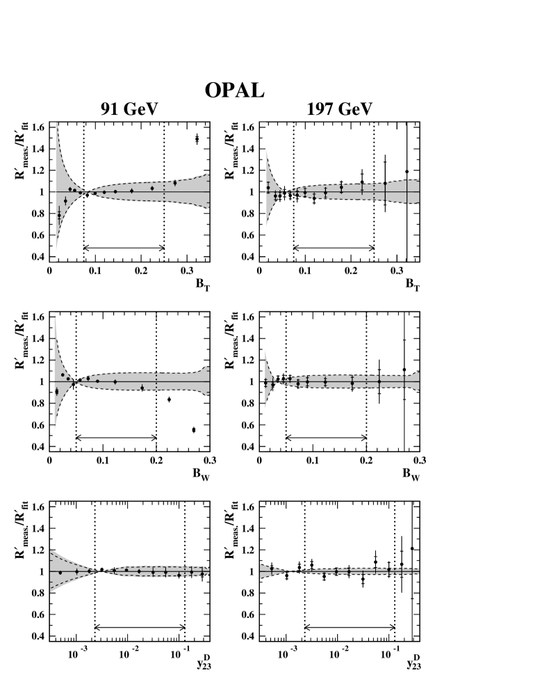
Figure 20: Fits of $\alpha_{\mathrm{s}}$ to event shape distributions for $B_{\mathrm{T}}$, $B_{\mathrm{W}}$ and $y^{\mathrm{D}}_{23}$ at 91 GeV and 197 GeV (i.e. combined 189–209 GeV). Each data point shows the measured bin contents divided by the integral of the predicted distribution across the bin; the inner error bars indicate statistical uncertainties, and the outer bars show the combined statistical and experimental contributions. The dashed curves represent fractional variations in the predicted distributions, corresponding to our perturbative theory uncertainties in $\alpha_{\mathrm{s}}$. The slightly wider shaded bands indicate the combined theory and hadronization uncertainties. The ranges used for fitting each distribution are shown by horizontal arrows.

Figure 26: The ratio $K=\mathcal{B}_{n}/\mathcal{A}_{n}$ of NLO and LO coefficients for the six observables used in our determinations of $\alpha_{\mathrm{s}}(M_{\mathrm{Z}})$ from moments.

References

- [1] R.K. Ellis, W.J. Stirling and B.R. Webber, “QCD and Collider Physics”, Cambridge University Press (1996).
- [2] OPAL Collab., P.D. Acton et al., Z. Phys. C59 (1993) 1.
- [3] OPAL Collab., G. Alexander et al., Z. Phys. C72 (1996) 191.
- [4] OPAL Collab., K. Ackerstaff et al., Z. Phys. C75 (1997) 193.
- [5] OPAL Collab., G. Abbiendi et al., Eur. Phys. J. C16 (2000) 185.
- [6] ALEPH Collab., D. Busculic et al., Z. Phys. C73 (1997) 409.
- [7] ALEPH Collab., A. Heister et al., Eur. Phys. J. C35 (2004) 457.
- [8] DELPHI Collab., P. Abreu et al., Z. Phys. C73 (1997) 229.
- [9] DELPHI Collab., P. Abreu et al., Phys. Lett. B456 (1999) 322.
- [10] DELPHI Collab., J. Abdallah et al., Eur. Phys. J. C29 (2003) 285.
- [11] L3 Collab., M. Acciarri et al., Phys. Lett. B371 (1996) 137.
- [12] L3 Collab., M. Acciarri et al., Phys. Lett. B404 (1997) 390.
- [13] L3 Collab., M. Acciarri et al., Phys. Lett. B444 (1998) 569.
- [14] L3 Collab., M. Acciarri et al., Phys. Lett. B489 (2000) 65.
- [15] L3 Collab., P. Achard et al., Phys. Lett. B536 (2002) 217.
- [16] OPAL Collab., G. Abbiendi et al., submitted to Eur. Phys. J. C.
-
[17]
OPAL Collab., K. Ahmet et al., Nucl. Instrum. and Methods A305 (1991) 275;
S. Anderson et al., Nucl. Instrum. and Methods A403 (1998) 326;
G. Aguillion et al., Nucl. Instrum. and Methods A417 (1998) 266. - [18] T. Sjöstrand, Comput. Phys. Commun. 82 (1994) 74.
-
[19]
S. Jadach, B.F.L. Ward and Z. Wa̧s, Phys. Lett. B449 (1999) 97;
S. Jadach et al., Comput. Phys. Commun. 130 (2000) 260. -
[20]
G. Marchesini et al., Comput. Phys. Commun. 67 (1992) 465;
G. Corcella et al., JHEP 0101 (2001) 010. - [21] J. Fujimoto et al., Comput. Phys. Commun. 100 (1997) 128.
- [22] S. Jadach et al., Comput. Phys. Commun. 119 (1999) 272.
- [23] J. Allison et al., Nucl. Instrum. Methods A317 (1992) 47.
- [24] L. Lönnblad, Comput. Phys. Commun. 71 (1992) 15.
- [25] OPAL Collab., G. Alexander et al., Z. Phys. C69 (1996) 543.
- [26] OPAL Collab., G. Abbiendi et al., Eur. Phys. J. C35 (2004) 293.
- [27] S. Brandt et al., Phys. Lett. 12 (1964) 57.
- [28] E. Fahri, Phys. Rev. Lett. 39 (1977) 1587.
- [29] D.P. Barber et al., Phys. Rev. Lett. 43 (1979) 830.
- [30] J.D. Bjorken and S.J. Brodsky, Phys. Rev. D1 (1970) 1416.
- [31] SLAC-LBL Collab., G. Hanson et al., Phys. Rev. Lett. 35 (1975) 1609.
- [32] S.L. Wu and G. Zobernig, Z. Phys. C2 (1979) 107.
-
[33]
G. Parisi, Phys. Lett. B74 (1978) 65;
J.F. Donoghue, F.E. Low and S.Y. Pi, Phys. Rev. D20 (1979) 2759;
R.K. Ellis, D.A. Ross and A.E. Terrano, Nucl. Phys. B178 (1981) 421. - [34] T. Chandramohan and L. Clavelli, Nucl. Phys. B184 (1981) 365.
- [35] L. Clavelli and D. Wyler, Phys. Lett. B103 (1981) 383.
- [36] S. Catani, G. Turnock and B.R. Webber, Phys. Lett. B295 (1992) 269.
- [37] S. Catani et al., Phys. Lett. B269 (1991) 432.
- [38] R.K. Ellis, D.A. Ross and A.E. Terrano, Nucl. Phys. B178 (1981) 421.
- [39] R.W.L. Jones et al., JHEP 12 (2003) 007.
- [40] S. Catani, L. Trentadue, G. Turnock and B.R. Webber, Nucl. Phys. B407 (1993) 3.
- [41] Yu.L. Dokshitzer, A. Lucenti, G. Marchesini and G.P. Salam, JHEP01 (1998) 011.
- [42] A. Banfi, G.P. Salam and G. Zanderighi, JHEP01 (2002) 018.
- [43] S. Catani and B.R. Webber, Phys. Lett. B427 (1998) 377.
- [44] S. Catani, G. Turnock and B.R. Webber, Phys. Lett. B295 (1992) 269.
- [45] G. Dissertori and M. Schmelling, Phys. Lett. B361 (1995) 167.
- [46] S. Catani et al., Phys. Lett. B269 (1991) 432.
- [47] S. Catani and M.H. Seymour, Phys. Lett. B378 (1996) 287.
- [48] Z. Kunszt and P. Nason [convenors], in “Z Physics at LEP I ” (eds. G. Altarelli, R. Kleiss and C. Verzegnassi ), CERN 89-08 (1989).
- [49] OPAL Collab., G. Alexander et al., Z. Phys. C52 (1991) 175.
- [50] OPAL Collab., G. Abbiendi et al., Eur. Phys. J. C33 (2004) 173.
- [51] OPAL Collab., G. Abbiendi et al., Phys. Lett. B493 (2000) 249.
- [52] G.D. Lafferty and T.R. Wyatt, Nucl. Instrum. and Methods A355 (1995) 541.
- [53] ALEPH, DELPHI, L3 and OPAL Collaborations and the LEP QCD Working Group, Paper in preparation.
- [54] Particle Data Group, S. Eidelman et al., Phys. Lett. B592 (2004) 1.