Application of Genetic Programming to High Energy Physics Event Selection

Abstract

We review genetic programming principles, their application to FOCUS data samples, and use the method to study the doubly Cabibbo suppressed decay $\mbox{{D}}^{+}\to\mbox{{K}}^{+}\pi^{+}\pi^{-}$ relative to its Cabibbo favored counterpart, $\mbox{{D}}^{+}\to\mbox{{K}}^{-}\pi^{+}\pi^{+}$. We find that this technique is able to improve upon more traditional analysis methods. To our knowledge, this is the first application of the genetic programming technique to High Energy Physics data.

The FOCUS Collaboration

See http://www-focus.fnal.gov/authors.html for additional author information.

1 Introduction

Genetic programming is one of a number of machine learning techniques in which a computer program is given the elements of possible solutions to the problem. This program, through a feedback mechanism, attempts to discover the best solution to the problem at hand, based on the programmers definition of success. Genetic programming differs from machine learning solutions such as genetic algorithms and neural networks in that the form or scope of the solution is not specified in advance, but is determined by the complexity of the problem. We have applied this technique to the study of a doubly Cabibbo suppressed branching ratio of $\mbox{{D}}^{+}$ since this measurement is presumed to be reasonably free of Monte Carlo related systematic errors. To our knowledge, this is the first application of the genetic programming technique to high energy physics data, although we have recently become aware of a Monte Carlo study [1] for the ATLAS experiment.

First, we review the basics of genetic programming and explain how genetic programming is used on FOCUS data. Next, we show the results of applying genetic programming techniques to the doubly Cabibbo suppressed decay $\mbox{{D}}^{+}\to\mbox{{K}}^{+}\pi^{+}\pi^{-}$, measure its branching ratio relative to the Cabibbo favored decay, and compare our results with a published analysis using more conventional methods. Finally, we describe studies of systematic errors related to the genetic programming method.

2 Introduction to Genetic Programming

We have adopted the tree representation and nomenclature of Koza [2] as our genetic programming model. Throughout this paper, we will use the terms “tree,” “program,” and “individual” interchangeably. Other, more general, representations also exist [3]. The specific implementation used is lil-gp [4] from the Michigan State University GARAGe group [5]. In this representation, the Genetic Programming Framework (GPF) creates a program which consists of a series of linked nodes. Each node takes a number of arguments and supplies a single return value. There are two general types of nodes: functions (or operators) and terminals (variables and constants). Functions take one or more input variables; terminals take no inputs and supply a single value to the program. In practice, the argument and return “values” can be any data structure, but in our case they are single floating point numbers.

This series of linked nodes can be represented as a tree where the leaves of the tree represent terminals and operators reside at the forks of the tree. For example, Fig. 1 shows the representation of the function ($p\times p)-(p+40)$. To “read” trees in this fashion, one resolves the sub-trees in a bottom-up fashion.

$-$ $\times$$p$$p$ $+$$p$$40$

Figure 1: Tree representation of the equation $(p\times p)-(p+40)$.

The genetic programming model seeks to mimic the biological processes of evolution, treating each of these trees or programs as an “organism.” Through natural selection and reproduction over a number of generations, the fitness (i.e., how well the program solves the specified problem) of a population of organisms is improved.

The process of determining the best (or nearly best) solution to a problem in genetic programming involves a series of steps:

1. Generate an initial population of “programs” to be evaluated.

2. Determine the fitness of each of these programs in solving the problem at hand.

3. Select which of these programs are allowed to contribute to the next generation.

4. Using these selected programs, generate the next generation using biological models.

5. Repeat steps 2–4 a number of times.

6. Terminate and evaluate the best solution(s).

2.1 Initial tree generation

The initial trees to be evaluated are created in one of two ways. The first, termed “grow,” randomly selects either a terminal or a function as the first (top) node in the tree. If a function is selected, the “child” nodes required by that function are again randomly selected from either functions or terminals. Growth is stopped either when all available nodes have been filled with terminals or when the maximum depth (measured from top to bottom) for the tree is reached (at which point only terminals are chosen).

The second method, termed “full,” proceeds similarly, except only functions are chosen at levels less than the desired depth of the initial tree and only terminals are selected at the desired depth. Typically one specifies a range of depths, which results in subpopulations of differing complexity.

In the initial generation, every tree in the population is guaranteed to be unique. Later generations are allowed to have duplicate individuals.

For a wide range of problems it has been observed that generating half the initial population with the grow method and the other half with various depths of full trees provides a good balance in generating the initial population.

2.2 Fitness evaluation

Central to genetic programming is the idea of fitness. Fitness is the measure of how well the program, or tree, solves the problem presented by the user. The GPF we use requires the calculation of standardized fitness such that the best possible solution will have a fitness of 0 and all other solutions will have positive fitness values. The exact definition of the standardized fitness is left to the programmer.

Another useful quantity is the adjusted fitness,

$$f_{a}(i)=\frac{1}{1+f_{s}(i)}$$ (1)

where $f_{a}(i)$ is the adjusted fitness of the $i^{\text{th}}$ individual and $f_{s}(i)$ is the standardized fitness of the same individual. One can readily see that as $f_{s}$ decreases, $f_{a}$ increases to a maximum of 1.0.

2.3 Survival selection

To mimic the evolutionary process of natural selection, the probability that a particular tree will pass some of its “genetic material,” or instructions, on to the next generation must be proportional in some way to the fitness of that individual.

In genetic programming, several kinds of selection are employed. The first is “fitness-proportionate,” in which the probability, $p_{i}$, of selection of the $i^{\text{th}}$ individual is

$$p_{i}=\frac{f_{a}(i)}{\sum_{j}f_{a}(j)}$$ (2)

where $j$ sums over all the individuals in a population. In this way, very fit individuals are selected more often than relatively unfit individuals. This is the most common method of selection in genetic programming.

For complicated problems which require larger population sizes, “fitness-over-selection” is often used. In this method, the population is divided into two groups, a small group of “good” individuals and a larger group of the remaining individuals. The majority of the time, an individual is selected from the smaller group, using the rules for fitness-proportionate selection. The rest of the time, the individual is selected from the larger group, again with the same rules.

In our implementation, the small group contains the best individuals which account for (320/population size) of the total adjusted fitness. E.g., for a population size of 4000, the small group contains the individuals summing to 8% of the total adjusted fitness. Individuals are selected from this small group 80% of the time.

Additional types of selection are sometimes used in genetic programming. These include “tournament,” in which two or more individuals are randomly chosen and the best is selected, and “best,” in which the best individuals are selected in order.

2.4 Breeding algorithms

The process of creating a new generation of programs from the preceding generation is called “breeding” in the genetic programming literature. The similar sounding term, “reproduction,” is used in a specific context as explained below.

The methods used to produce new individuals are determined randomly; more than one method can be (and is) used. Each of these methods must select one or more individuals as “parents.” The parents are selected according to the methods described above. The GPF we are using implements three such methods: reproduction, crossover, and mutation. Other methods, e.g. permutation, also exist [2].

2.4.1 Reproduction

“Reproduction” might also be called cloning or asexual reproduction. The selected individual is simply copied into the next generation without alteration.

2.4.2 Crossover

“Crossover,” or sexual reproduction, randomly selects two parent trees and creates two new trees. In an attempt to mimic DNA exchange between two parents, a node is selected on each tree, those nodes and all child nodes are removed from the parent trees and inserted into the vacant spot in the other tree. This process is illustrated in Fig. 2.

$-$ [linestyle=dashed]$\times$$p$$p$ $+$$p$$40$

(a) 1${}^{\text{st}}$ parent

$+$ $/$$p_{T}$$L$ [linestyle=dashed]$\cos$$p$

(b) 2${}^{\text{nd}}$ parent

$-$ $\cos$$p$ $+$$p$$40$

(c) 1${}^{\text{st}}$ child

$+$ $/$$p_{T}$$L$ $\times$$p$$p$

(d) 2${}^{\text{nd}}$ child

Figure 2: Example of crossover. Shown are the two parents (a) and (b) and the two resulting children (c) and (d). The crossover points chosen are designated with the dashed ovals.

2.4.3 Mutation

In mutation, a single parent is selected. A node on the tree is selected, the existing contents and any child nodes are destroyed, and a new node (terminal or function) is inserted in its place. New nodes are inserted following the rules for growing the initial trees. Both the tree and mutation point are selected randomly. An example of mutation is shown in Fig. 3.

$-$ $\times$$p$$p$ $+$$p$[linestyle=dashed]$40$

(a) Parent

$-$ $\times$$p$$p$ $+$$p$$-$$L$$p_{T}$

(b) Mutated child

Figure 3: Example of mutation. Shown are the parent (a) and the resulting child (b). The mutation point is denoted by the dashed oval.

Typically the amount of mutation is kept small since it is exploring new parameter space, not parameter space that has proven to be interesting already. However, as in biological processes, mutation may be important to preserve or increase diversity. Note that mutation beginning with the first node is equivalent to generating a completely new individual.

2.5 Migration

Although not part of early genetic programming models, we use migration of individuals as an important element of generating diversity. In our parallel genetic programming model, sub-populations (or “islands”) are allowed to evolve independently with exchanges between sub-populations taking place every few generations. Every $n_{g}$ generations, the best $n_{i}$ individuals from each sub-population are copied into every other sub-population. After this copying, they may be selected by the methods discussed above for the various breeding processes.

This modification to the method allows for very large effective population to be spread over a large number of computers in a network.

2.6 Termination

When the required number of generations have been run and all the individuals evaluated, the GPF terminates. At this point, a text representation of the best tree (not necessarily from the last generation) is written out and other cleanup tasks are performed.

3 Combining Genetic Programming with High Energy Physics Data

While genetic programming techniques can be applied to a wide variety of problems in High Energy Physics (HEP), we illustrate the technique on the common problem of event selection: the process of distinguishing signal events from the more copious background processes. Event selection in HEP has typically been performed by what we will call the “cut method.” The physicist constructs a number of interesting variables, either representing kinematic observables or a statistical match between data and predictions. These variables are then individually required to be greater and/or less than some specified value. This increases the purity of the data sample at the expense of selection efficiency. Less commonly, techniques which combine these physics variables in pre-determined ways are included. Genetic programming makes no pre-supposition on the final form of a solution.

The charm photoproduction experiment FOCUS is an upgraded version of FNAL-E687 [6] which collected data using the Wideband photon beamline during the 1996–1997 Fermilab fixed-target run. The FOCUS experiment utilizes a forward multiparticle spectrometer to study charmed particles produced by the interaction of high energy photons ($\langle E\rangle\approx 180~{}\mathrm{GeV}$) with a segmented BeO target. Charged particles are tracked within the spectrometer by two silicon microvertex detector systems. One system is interleaved with the target segments [7]; the other is downstream of the target region. These detectors provide excellent separation of the production and decay vertices. Further downstream, charged particles are tracked and momentum analyzed by a system of five multiwire proportional chambers [8] and two dipole magnets with opposite polarity. Three multicell threshold Čerenkov detectors are used to discriminate among electrons, pions, kaons, and protons [9]. The experiment also contains a complement of hadronic and electromagnetic calorimeters and muon detectors.

To apply the genetic programming technique to FOCUS charm data, we begin by identifying a number of variables which may be useful for separating charm from non-charm. We also identify variables which may separate the decays of interest from other charm decays. Many of the variables selected are those we use as cuts in traditional analyses, but since genetic programming combines variables not in cuts, but in an algorithmic fashion, we also include a number of variables that may be weak indicators of charm or the specific decay in question. For instance, we have included variables that attempt to provide an indicator of opposite (or away) side charm.

3.1 Definition of Fitness

For the doubly Cabibbo suppressed decay $\mbox{{D}}^{+}\to\mbox{{K}}^{+}\pi^{+}\pi^{-}$, we are looking for very small signals. The fitness of a tree, as returned to the GPF, describes how small the error on a measurement of $\text{BR}(\mbox{{D}}^{+}\to\mbox{{K}}^{+}\pi^{+}\pi^{-})/\text{BR}(\mbox{{D}}^{+}\to\mbox{{K}}^{-}\pi^{+}\pi^{+})$ will be.

We would like to maximize the expected significance of the possible signal, $S_{\text{DCS}}/\sqrt{S_{\text{DCS}}+B_{\text{DCS}}}$, where $S_{\text{DCS}}$ and $B_{\text{DCS}}$ are the doubly Cabibbo suppressed signal and background, respectively. However, with a small number of signal events and a very large search space, this method is almost guaranteed to optimize on fluctuations. Instead, one may choose to predict the number of signal events, $S_{\text{DCS}}$, from the behavior of the corresponding Cabibbo favored decay mode. In our test of this method on $\mbox{{D}}^{+}\to\mbox{{K}}^{+}\pi^{+}\pi^{-}$, we use the PDG branching ratio to estimate our sensitivity. Assuming equal selection efficiencies, $S_{\text{CF}}$ (the signal yield in the Cabibbo favored mode) is proportional to the predicted number of doubly Cabibbo suppressed events. $S_{\text{CF}}$ is determined by a fit to the Cabibbo favored invariant mass distribution and $B_{\text{DCS}}$ is determined by a linear fit over the background range (excluding the signal region) in the doubly Cabibbo suppressed invariant mass distribution.

However, because we are still optimizing based on $B$ from the doubly Cabibbo suppressed mass plot, we must be concerned about causing downward fluctuations in $B_{\text{DCS}}$ which would appear to improve our significance. (To a much lesser extent, we must be concerned about upwardly fluctuating the Cabibbo favored signal.) We address this in two ways. First, we apply a penalty to the fitness (or significance) based on the size of the tree; i.e., we attempt to ensure that any increase in the tree size is making a significant contribution to reducing the background (or increasing the signal), not just changing a few events. Second, we optimize the significance only on even-numbered events. We can then look at the odd-numbered events to assess any biases.

Because the genetic programming framework is set up to minimize, rather than maximize, the fitness and because we want to enhance differences between small changes in significance, we minimize the quantity

$$\frac{S_{\text{pred}}+B_{\text{DCS}}}{S_{\text{CF}}^{2}}\times 10,000\times(1+0.005\times\text{\# of nodes})$$ (3)

where

$$S_{\text{pred}}=S_{\text{CF}}\times\frac{\text{BR}(\mbox{{D}}^{+}\to\mbox{{K}}^{+}\pi^{+}\pi^{-})}{\text{BR}(\mbox{{D}}^{+}\to\mbox{{K}}^{-}\pi^{+}\pi^{+})}\,.$$ (4)

The relative branching ratio is taken from the PDG. This penalty factor of 0.5% per node is arbitrary and is included to encourage the production of simpler trees. This is more fully explained in Section 6.3. Squaring $\sqrt{S+B}/S$ emphasizes differences between trees and multiplying by 10,000 ensures that the average fitness is $\mathcal{O}(1)$.

Finally, we make two additional constraints. We require that at least 500 events, in Cabibbo favored and doubly Cabibbo suppressed modes combined, are selected. We also require that the Cabibbo favored signal be observed at the $6\sigma$ level. Both of these requirements ensure that a good Cabibbo favored signal exists. Trees which fail these requirements are assigned a fitness of 100, a very poor fitness.

While it would be preferable to maximize $S/\sqrt{S+B}$ on signal and background from Monte Carlo, there are a number of problems with this. First, we know that our Monte Carlo does not reproduce backgrounds particularly well since non-charm backgrounds are not simulated. Second, we aren’t sure the Monte Carlo reproduces all the kinematic and other parameters of our charm signals correctly, and we certainly don’t know that the Monte Carlo would reproduce them correctly in all the combinations the GPF could create. We can make limited tests of this agreement on the final product, as discussed in Section 6.1. However, because the two Cabibbo favored and doubly Cabibbo suppressed decay modes under study are so similar in particle ID and kinematics, we believe we are justified in assuming that they will behave nearly identically under various programs suggested by the GPF.

3.2 Functions and Variables

We supply a wide variety of functions and variables to the GPF which can be used to construct trees. The constructed tree is evaluated for every combination. Events for which the tree returns a value greater than zero are kept. Fits are made to determine $S_{\text{CF}}$ and $B_{\text{DCS}}$.

Mathematical Functions and Operators: The first group of functions are standard mathematical (algebraic and trigonometric) functions and operators. Every function must be valid for all possible input values, so division by zero and square roots of negative numbers must be allowed. These mathematical functions and the protections used are shown in Table 1.

Table 1: Mathematical functions and operators. $f(n)$ is the sigmoid function commonly used in neural networks.

Operator	Description
$+$
$-$
$\times$
$/$	Divide by 0 $\to$ 1
$x^{y}$	$x$ is 1${}^{\text{st}}$ argument, $y$ is second
$\log$	$\log\left|x\right|$, $\log 0=0$
$\sin$
$\cos$
$\sqrt{\vphantom{\left|x\right|}\ }$	$\sqrt{\left|x\right|}$
neg	negative of $x$
sign	returns $(-1,0,+1)$
$f(n)$	$1/\left(1+e^{-n}\right)$
$\max$	Maximum of two values
$\min$	Minimum of two values

Boolean Operators: We also use a number of Boolean operators. Our Boolean operators must take all floating point values as inputs. We define any number greater than zero as “true” and any other number as “false.” Boolean operators return 1 for “true” and 0 for “false.” The IF operator is special; it returns the value of its second operand if the value of its first operand is true; otherwise it returns zero (or false). We also use the comparison operator, $<\!=\!>$, as defined in the Perl programming language [10, pg. 87]. This operator returns $-1$ if the first value is less than the second, $+1$ if the opposite is true, and $0$ if the two values are equal. The Boolean operators are listed in Table 2.

Table 2: Boolean operators and the comparison operator.

Operator	Description
$>$
$<$
AND
OR
NOT
XOR	True if one and only one operand is true
IF	2${}^{\text{nd}}$ value if 1${}^{\text{st}}$ true, 0 if false
$<\!=\!>$	$>\to+1$, $<\to-1$, $=\to 0$

A large number of variables, or terminals, are also supplied. These can be classified into several groups: 1) vertexing and tracking, 2) kinematic variables, 3) particle ID, 4) opposite side tagging, and 5) constants. All variables have been redefined as dimensionless quantities.

Vertexing Variables: The vertexing and tracking variables are mostly those used in traditional analyses [6]: $\ell/\sigma_{\ell}$, isolation cuts, vertex CLs and isolations, etc. The tracking $\chi^{2}$ variables which are calculated by the wire chamber tracking code [8] are not generally used in analyses. The vertexing and tracking variables are shown in Table 3.

Table 3: Vertexing and tracking variables. The tracking $\chi^{2}$ variables differ by species.

Variable	Units	Description
$\ell$	cm	Distance between production and decay vertices
$\sigma_{\ell}$	cm	Error on $\ell$
$\ell/\sigma_{\ell}$	—	Significance of separation between vertices
ISO1, ISO2	—	Isolation of production and decay vertices
OoM	$\sigma$	Decay vertex out of material
POT	$\sigma$	Production vertex out of target
CLP, CLS	—	CL of production and decay vertices
$\sigma_{t}$	ps	Lifetime resolution
$\chi^{2}_{K}$, $\chi^{2}_{\pi_{1}}$, $\chi^{2}_{\pi_{2}}$	—	Track $\chi^{2}$ for K, $\pi$, $\pi$

Kinematic Variables: Of the kinematic variables, most are familiar in HEP analyses. The most prominent exception is $\Sigma p_{T}^{2}$ which is the sum of the squares of the daughter momenta perpendicular to the charmed parent direction. When large, this variable means the invariant mass of the parent particle is generated by large opening angles rather than highly asymmetric momenta of the daughter particles. In this category, we also include the binary variables NoTS and TS which represent running before and after the installation of a second silicon strip detector [7]. The kinematic variables are shown in Table 4.

Table 4: Kinematic variables.

Variable	Units	Description
$\#\tau$	—	Lifetime/mean lifetime
$p$	$\mathrm{GeV}/c$	Charm momentum
$p_{T}$	$\mathrm{GeV}/c$	$p$ transverse to beam
$\Sigma p_{T}^{2}$	$\text{GeV}^{2}/c^{2}$	Sum of daughter $p_{T}^{2}$ (see text)
$m_{\text{err}}$	$\mathrm{MeV}/c^{2}$	Error on reconstructed mass
TS	0, 1	Early, late running
NoTS	0, 1	Opposite of TS

Particle Identification: For particle ID, we use the standard FOCUS Čerenkov variables [9] for identifying protons, kaons, and pions. We also include Boolean values from the silicon strip tracking code for each of the tracks being consistent with an electron (zero-angle) and the maximum CL that one of the decay tracks is a muon. The particle ID input variables are shown in Table 5.

Table 5: Particle ID variables.

Variable	Units	Description
$\Delta\pi\mbox{{K}}_{1}$	—	K not $\pi$
$\pi_{\mathrm{con}}{}_{1}$	—	$\pi$ consistency, first pion
$\pi_{\mathrm{con}}{}_{2}$	—	$\pi$ consistency, second pion
$\mu_{\text{max}}$	—	Maximum $\mu$ CL of all tracks
$K_{e}$, $\pi_{e1}$, $\pi_{e2}$	0/1 (True/False)	Electron consistency from silicon tracker

Opposite Side Tagging: Since genetic programming needn’t cut on variables we have investigated some possible methods for opposite (or away) side tagging. Any cut on these tagging methods is too inefficient to be of any use, but combined with other variables, variables representing the probability of the presence of an opposite side decay may be useful. Three such variables were formed and investigated. The first attempts to construct charm vertices from tracks which are not part of the production or decay vertices. The best vertex is chosen based on its confidence level. The second general method of opposite side tagging is to look for kaons or muons from charm decays that are not part of the decay vertex. (Here, tracks in the production vertex are included since often the production and opposite side charm vertices merge.) We determine the confidence level of the best muon of the correct charge and the kaonicity of the best kaon of the correct charge not in the decay vertex. The variables for opposite side charm tagging are shown in Table 6.

Table 6: Opposite side tagging variables.

Variable	Units	Description
$\text{CL}_{\text{opp}}$	—	CL of highest vertex opposite
$\Delta W(\pi\mbox{{K}})_{\text{opp}}$	—	Highest kaonicity not in secondary
$\text{CL}\mu_{\text{opp}}$	—	Highest muon CL not in secondary

Constants: In addition to these variables, we also supply a number of constants. We explicitly include 0 (false) and 1 (true) and allow the GPF to pick real constants on the interval $(-2,+2)$ and integer constants on the interval $(-10,+10)$.

The optimization in this example uses 21 operators or functions and 34 terminals (variables or constants).

3.3 Anatomy of a Run

Once we have defined all of our functions and terminals and defined the fitness, we are ready to start the GPF. To recap, the steps taken by the GPF are:

1. Generate a population of individual programs to be tested.

2. Loop over and calculate the fitness of each of these programs.

   1. Loop over each physics event.

   2. Keep events where the tree evaluates to $>0$, discard other events.

   3. For surviving events, fit the Cabibbo favored signal and doubly Cabibbo suppressed background.

   4. Return the fitness calculated according to Eq. (3).

3. When all programs of a generation have been tested, create another generation by selecting programs for breeding according to the selection method. Apply breeding operators such as cross-over, mutation, and reproduction.

4. Every few generations, exchange the best individuals among “islands.”

5. Continue, repeating steps 2–4 until the desired number of generations is reached.

4 Selecting Genetic Programming Parameters

There are a large number of parameters that can be chosen within the GPF, such as numbers of individuals, selection probabilities, and breeding probabilities. Each of these can affect the evolution rate of the model and affect the probability that the initial individuals don’t have enough diversity to reliably find a good minimum. It should be emphasized, though, that the final result, given enough time, should not be affected by these choices (assuming sufficient diversity). The default parameters for the studies presented in this section are given in Table 7.

Table 7: Default genetic programming parameters for studies.

Parameter	Value
Generations	6
Programs/sub-population	1000
Sub-populations	20
Exchange interval	2 generations
Number exchanged	5
Selection method	Fitness-over-select
Cross-over probability	0.85
Reproduction probability	0.10
Mutation probability	0.05
Generation method	Half grow, half full
Full depths	2–6
Maximum depth	17

In monitoring our test runs, we look at the fitness and size of each individual. We only consider individuals which have a fitness less than about 3 times worse than the fitness of a single-node tree which selects all events. This excludes individuals where no events were selected and others where much more signal than background was removed. We then look at average and best fitness as a function of generation while we vary various parameters of the genetic programming run.

In Fig. 4 we show the effects of various ways of doubling the total number of programs examined by the genetic programming run. We begin with a run on 20 sub-populations with 1000 individuals per sub-population and lasting 6 generations. We then double each of these quantities. One can see that either doubling the sub-population size or doubling the number of sub-populations gives about the same best and average fitness as the original case. However, doubling the number of generations has a significant effect on the average and best fitness of the population. After 12 generations (plus the initial generation “0”), evolution is still clearly occurring.

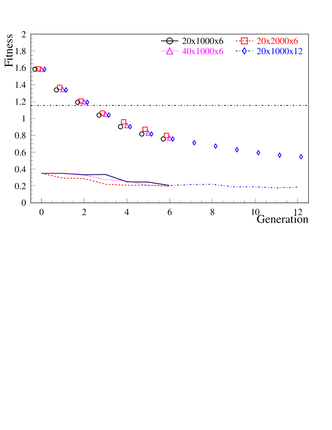
Figure 4: Plots of fitness vs. generation for increased statistics. The points show the average fitness for a generation and the curves show the fitness of the best individual. The straight line shows the fitness of the initial sample. The circles and solid line show the initial conditions: 20 sub-populations, 1000 individuals per sub-population, and 6 generations. The squares and dashed line show the effect of doubling the individuals per sub-population to 2000. The triangles and dotted line show the effect of doubling the sub-populations to 40. The diamonds and dotted-dashed line show the effect of doubling the number of generations to 12.

In addition to changing the number of individuals evaluated during the genetic programming run as discussed above, there are a number of parameters in the genetic programming framework that can be adjusted. These may change the rate or ultimate end-point of the evolution.

In Fig. 5 we show the effect of changing some of the basic parameters of the genetic programming framework on the evolution of the population. These plots show the effect over 12 generations of changing the selection method, the number of programs exchanged during the migration phase, and the size of the initial programs generated.

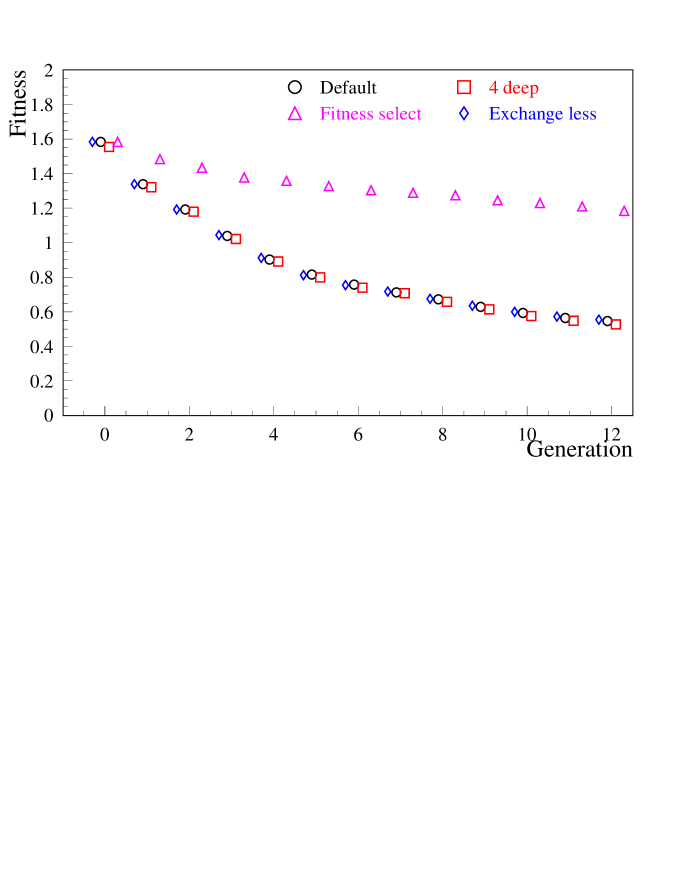
Figure 5: Plots of fitness vs. generation for different GP parameters. The points show the average fitness for a generation. The circles show the default settings. The squares show the effect of changing the “full” part of the initial population generation to produce trees with depths of 2–4 (rather than the default 2–6). The diamonds show the effect of exchanging 2 rather than 5 individuals per process in the migration phase. The triangles show the effect of using “fitness” rather than “fitness over-select” selection. (The fitness over-select method is used in all other plots.)

Exchanging 2 rather than 5 individuals from each process every 2 generations results in no change in the evolution rate. (For the standard case where we have 20 CPUs each with a population of 1000, exchanging 5 individuals from each of 20 CPUs means that 10% of the resulting sub-population is in common with each other sub-population.)

Changing the selection method used has a dramatic effect on the evolution. Changing from our default “fitness-over-select” method to the more common “fitness” method results in a much more slowly evolving population. Recall that in the standard fitness selection, the probability of an individual being selected to breed is directly proportional to the fraction of the total fitness of the population accounted for by the individual. In the fitness-over-select method, individuals in the population are segregated into two groups based on their fitness. Individuals which breed are selected more often from the more fit group (which also tends to be smaller). Selection within each group is done in the same way as for the standard fitness selection method.

Conventional wisdom is that fitness-over-selection can be useful for large populations (larger than about 500 individuals). For smaller populations, there are risks associated with finding local minima.

As discussed in Section 2.1, half of the trees are generated by the “full” generation method. In the default evolution plot shown in Fig. 5, the beginning depths of these trees are from 2 to 6. So, 10% of the initial trees are of depth 2, 10% are of depth 3, etc., up to 10% of depth 6. The remaining 50% are generated by the “grow” method. As can be seen, changing the depth of the full trees so that trees of depth 5 and 6 are not allowed has little effect on the evolution rate. Other, earlier studies indicate that this change may positively affect the fitness in early generations and negatively affect the fitness of the later generations.

Fig. 6 shows the effect of changing the mutation probabilities. Increasing the mutation probability from 5% to 10% (at the expense of the crossover probability) does very little to change the evolution rate. Reducing the mutation probability to 2.5% or even 0% has a similarly small effect. However, at higher mutation rates, we worry about the effects of too high a mutation rate on later generations where stability should be increasing.

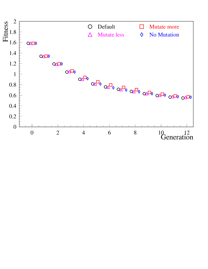
Figure 6: Plots of fitness vs. generation for different mutation rates. The points show the average fitness for a generation. The circles and show the default settings. The squares show the effect of doubling the mutation probability from 5% to 10%, the triangles show the effect of halving the mutation probability from 5% to 2.5%, and the diamonds show the effect of eliminating mutation.

Fig. 7 shows the effect of reducing the number of functions used in the search. In the first case, we removed a number of the algebraic, trigonometric, logical, and arithmetic operators. Operators such as $\log$, $x^{y}$, $\sin$, $\cos$, XOR, and others were not allowed to be used. This reduces the diversity of the program set, but may allow a minimum to be found faster if those operators are not necessary. In another trial, we removed variables not normally used in FOCUS analyses, such as opposite side tagging, track CLs, muon and electron mis-ID for hadrons, etc. In a final trial we removed both non-standard variables and questionable functions. The assumption in all three cases is the same: if the functions or variables added to the minimal case do not positively contribute to the overall fitness, slower evolution and possibly a worse final solution should be observed since the useful parameter space is less well covered. That this is not observed in the average case (which is less susceptible to fluctuations) suggests that the “extra” functions and variables are useful and ultimately better solutions may be found by including them.

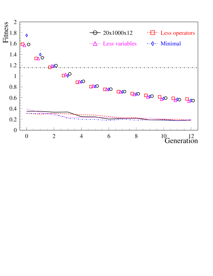
Figure 7: Plots of average and best fitness vs. generation for sets of reduced functions. For “Less operators,” (squares and dashed line) the set of arithmetic, algebraic, and logical operators was reduced to a minimal set. For “Less Variables” (triangles and dotted line) only “standard” analysis variables were included. For “Minimal” (diamonds and dashed-dotted line) both reductions were employed.

For all the studies detailed so far, we used a data sample with a relatively strict cut of $\ell/\sigma_{\ell}>15$. This is a very powerful cut and is an easy way to obtain a small, highly enriched sample of D mesons, speeding up the studies. However, the goal of our use of the genetic programming method is to try to discover ways around making such tight cuts. Fig. 8 shows the effect of changing the cut on the initial data sample to $\ell/\sigma_{\ell}>10$. One sees that while initially the best individuals are not as pure as the $\ell/\sigma_{\ell}>15$ sample, parity is quickly reached. It’s reasonable to assume that in later generations, the $\ell/\sigma_{\ell}>10$ selection becomes more effective as events with $10<\ell/\sigma_{\ell}<15$ (about 7.5% of the total in the 12th generation) are included which have other indications of being $\mbox{{D}}^{+}\to\mbox{{K}}^{-}\pi^{+}\pi^{+}$ decays. (The plots of the average never reach the same level, but this is to be expected as the initial purity is not as good and many programs, even at later stages, do not perform any event selection. Because of this effect, comparing the averages of the two cases is not instructive.)

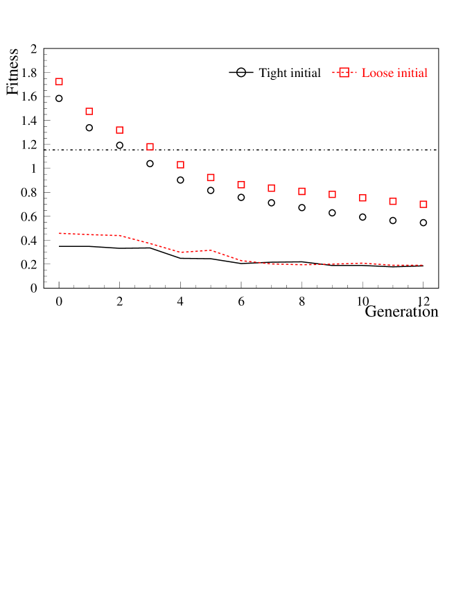
Figure 8: Plots of fitness vs. generation for different initial data samples. The default sample (circles and solid line) has a cut of $\ell/\sigma_{\ell}>15$ while the “Loose” sample has a cut of $\ell/\sigma_{\ell}>10$.

5 Testing Genetic Programming on $\mbox{{D}}^{+}\to\mbox{{K}}^{+}\pi^{+}\pi^{-}$

Having explored various settings in the GPF to determine the way to obtain the best evolution of programs, we now investigate the ultimate performance and accuracy of this method to measure the relative branching ratio $\text{BR}(\mbox{{D}}^{+}\to\mbox{{K}}^{+}\pi^{+}\pi^{-})/\text{BR}(\mbox{{D}}^{+}\to\mbox{{K}}^{-}\pi^{+}\pi^{+})$.

Recall from Eq. (3) that the GPF is attempting to minimize the quantity

$$\frac{B_{\text{DCS}}+S_{\text{pred}}}{S_{\text{CF}}^{2}}\times 10,000\times(1+0.005\times\text{\# of nodes})\,,$$ (5)

where $B_{\text{DCS}}$ is a fit to the background excluding the $\pm 2\sigma$ signal window and $S_{\text{pred}}$ is the expected doubly Cabibbo suppressed yield determined from the PDG value for the $\mbox{{D}}^{+}\to\mbox{{K}}^{+}\pi^{+}\pi^{-}$ relative branching ratio [11] and the Cabibbo favored signal ($S_{\text{CF}}$). We exclude from the fit the expected signal region in the doubly Cabibbo suppressed decay channel to avoid inflating $B_{\text{DCS}}$ (or alternatively allowing the GPF to learn how to eliminate the doubly Cabibbo suppressed signal).

To start with a data sample of manageable size, certain requirements must be enforced on the data supplied to the GPF. For the final runs looking for $\mbox{{D}}^{+}\to\mbox{{K}}^{+}\pi^{+}\pi^{-}$, these requirements are:

• $\ell/\sigma_{\ell}$ $>10$

• CLS $>0.01$

• $\pi_{\mathrm{con}}$ $>-8.0$ for both pions

• $\Delta W(\pi\mbox{{K}})$ $>1.0$ for kaon

• $1.75~{}\mathrm{GeV}/c^{2}<\text{Mass}<1.95~{}\mathrm{GeV}/c^{2}$

These requirements are applied to both $\mbox{{D}}^{+}\to\mbox{{K}}^{-}\pi^{+}\pi^{+}$ and $\mbox{{D}}^{+}\to\mbox{{K}}^{+}\pi^{+}\pi^{-}$ candidates.

The initial data sample is shown in Fig. 9. The Cabibbo favored signal dominates, and the level of doubly Cabibbo suppressed candidates (the linear histogram) is higher than the Cabibbo favored background. The Cabibbo favored fit finds $253\,180\pm 660$ events.

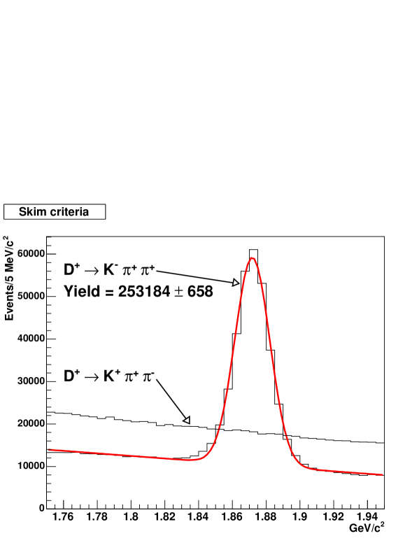
Figure 9: The initial $\mbox{{D}}^{+}\to\mbox{{K}}^{-}\pi^{+}\pi^{+}$ and $\mbox{{D}}^{+}\to\mbox{{K}}^{+}\pi^{+}\pi^{-}$ candidate distributions (the cuts are described in the text). The linear doubly Cabibbo suppressed invariant mass distribution is superimposed on the Cabibbo favored distribution. (No signal is visible.)

We select the $\mbox{{D}}^{+}\to\mbox{{K}}^{+}\pi^{+}\pi^{-}$ and $\mbox{{D}}^{+}\to\mbox{{K}}^{-}\pi^{+}\pi^{+}$ events using the genetic programming technique with the parameters listed in Table 8. These parameters are similar to those used in our earlier studies, but we increase the programs per generation and the number of generations.

Table 8: Genetic programming parameters for $\mbox{{D}}^{+}\to\mbox{{K}}^{+}\pi^{+}\pi^{-}$ optimization.

Parameter	Value
Generations	40
Programs/sub-population	1500
Sub-populations	20
Exchange interval	2 generations
Number exchanged	5
Selection method	Fitness-over-select
Cross-over probability	0.85
Reproduction probability	0.10
Mutation probability	0.05
Generation method	Half grow, half full
Full depths	2–6
Maximum depth	17

Fig. 10 shows the data after selection by the GPF for the Cabibbo favored and doubly Cabibbo suppressed decay modes. The GPF ran for 40 generations. A doubly Cabibbo suppressed signal is now clearly visible. $62\,440\pm 260$ (or about 25%) of the original Cabibbo favored events remain and $466\pm 36$ doubly Cabibbo suppressed events are now visible. The doubly Cabibbo suppressed background has been reduced by a factor greater than 150. All fits to doubly Cabibbo suppressed signals use the mass and resolution determined from the Cabibbo favored signals. The free parameters are the yield and the background shape and level.

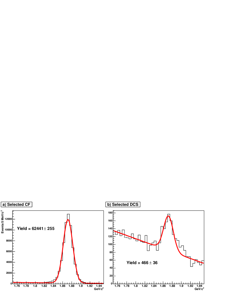
Figure 10: $\mbox{{D}}^{+}\to\mbox{{K}}^{-}\pi^{+}\pi^{+}$ (a) and $\mbox{{D}}^{+}\to\mbox{{K}}^{+}\pi^{+}\pi^{-}$ (b) signals selected by genetic programming. We find $62\,440\pm 260$ and $466\pm 36$ events, respectively.

The evolution of the individuals in the genetic programming is shown in Fig. 11. In addition to the variables plotted before, the average size for each generation is also plotted. We can see that the average size reaches a minimum at the 4th generation, nearly plateaus between the 20th and 30th generations, and then begins increasing again and is still increasing at the 40th generation.

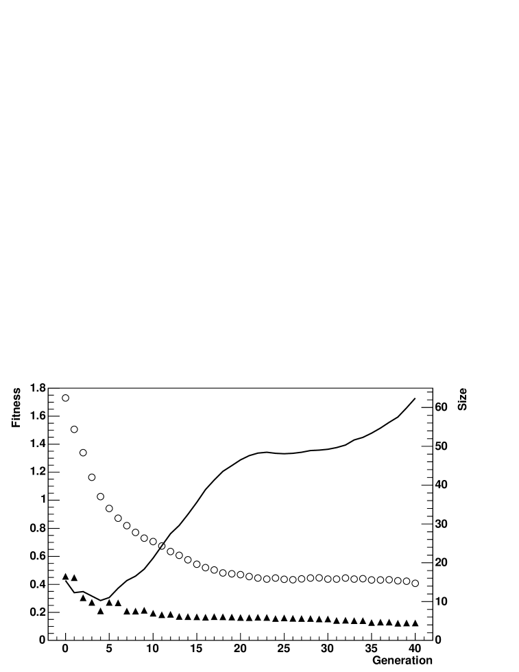
Figure 11: Evolution of $\mbox{{D}}^{+}\to\mbox{{K}}^{-}\pi^{+}\pi^{+}$ programs. The open circles show the average fitness of the population as a function of generation. The triangles show the fitness of the best individual. The solid line shows the average size of the individuals as a function of the generation.

In Fig. 11, the average and best fitnesses seems to stabilize, but in Fig. 12 an enlargement of the best fitness for later generations is seen. From this plot, it is apparent that evolution is still occurring at the 40th generation and new, better trees are still being found.

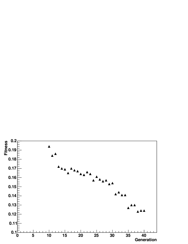
Figure 12: Expanded view of evolution of $\mbox{{D}}^{+}\to\mbox{{K}}^{-}\pi^{+}\pi^{+}$ programs. The triangles show the fitness of the best individuals for later generations, the same data as in Fig. 11, but on an expanded scale.

5.1 Example trees from various generations

In Fig. 13 we show four of the most fit trees from the initial generation (numbered 0); no evolution has taken place at this point. It is interesting to note several things. First, the best trees are all rather small, although the average tree in this generation is over 15 nodes in size. Second, the most fit tree in this generation (a) is recognizable to any FOCUS collaborator: it requires that the interaction vertex point be in the target and that the decay vertex point be located outside of target material. The second most fit tree (b) is algorithmically identical to the first, but has a slightly worse fitness because it is considerably larger than the first tree. Tree (c) is nearly identical in functionality to (a) and (b) but actually does a slightly better job of separating events than (a) or (b). Its fitness is slightly worse because of its larger size (12 nodes vs. 5 and 10 nodes respectively).

$\times$NOTPOTsignOoT

(a) Fitness 0.458

ANDXOR+1.900.44NOTOoTsignnegPOT

(b) Fitness 0.469

$<$$\sqrt{\ }$$<$-0.51POT$x^{y}$IFOoTClsOR$p$$K_{e}$

(c) Fitness 0.471

$<$minsign$\ell/\sigma_{\ell}$IFOoTPOTsign$>$$K_{e}$OSCL

(d) Fitness 0.472

Figure 13: The four most fit trees from generation 0 of a $\mbox{{D}}^{+}\to\mbox{{K}}^{+}\pi^{+}\pi^{-}$ run.

The four best individuals from generation 2 are shown in Fig. 14. A few observations are in order. First, the most fit tree (a) doesn’t include either of the elements we saw in the best trees in generation 0 (OoT and POT), but this tree is significantly more fit than any tree in generation 0. The second best tree (b) does include these elements, mixed in with others. Also, one can see that the fourth most fit tree (d) is quite large (44 nodes) compared to the other best trees in the generation.

$<\!=\!>$$-$$<$TS$\sigma_{t}$Iso1$f(n)$$\sigma_{t}$

(a) Fitness 0.305

$>$$x^{y}$$<\!=\!>$$<\!=\!>$OoT$\chi^{2}_{\pi 2}$/Iso1Clscossign$\chi^{2}_{\pi 1}$/POTCls

(b) Fitness 0.309

AND$\sigma_{t}$min$<$Iso1$\sigma M$IF$\chi^{2}_{\pi 1}$OoT

(c) Fitness 0.383

$\sqrt{\ }$IFXOR$>$/NOTsignIso2signcosTSNOTsign$>$OoT$K_{e}$neg$\times$$<$IF$\Sigma p^{2}_{T}$${\pi_{\mathrm{con}}}_{2}$$>$OS_μmax$\ell/\sigma_{\ell}$$p$$\sqrt{\ }$maxPOTPOT$\times$$<\!=\!>$$f(n)$$\#\tau$ANDClpKChiXORneg$\chi^{2}_{\pi 1}$$<$$\sigma_{\ell}$$\chi^{2}_{\pi 1}$

(d) Fitness 0.397

Figure 14: The four most fit trees from generation 2 of a $\mbox{{D}}^{+}\to\mbox{{K}}^{+}\pi^{+}\pi^{-}$ run.

As shown in Fig. 11, the average size tree of the population reaches a minimum in generation 4. One possible interpretation of this behavior is that at this point, the GPF has determined the parts of successful solutions. Going forward, it is assembling these parts into more complex solutions. The three best solutions from generation four are shown in Fig. 15. The best solution from generation four (a) is very similar to the best solution from generation two, but with the two end nodes replaced with new end nodes. The second and third best solutions are clearly related, with just one small difference: the second best tree (b), with the sub-branch: $\text{OS}_{\mu}<\!=\!>\text{OoT}$ only lets about 250 events with OoT $\leq 0$ through the filter while the third best tree (c) allows about 9300 such events through.

$<\!=\!>$$-$$<$0OoTIso1$f(n)$$\sigma_{t}$

(a) Fitness 0.211

$\times$$>$$x^{y}$$-$$\chi^{2}_{\pi 2}$Iso1Cls$<\!=\!>$OS_μOoTNOTPOT

(b) Fitness 0.272

$\times$$>$$x^{y}$$-$$\chi^{2}_{\pi 2}$Iso1ClsnegOoTNOTPOT

(c) Fitness 0.281

Figure 15: The three most fit trees from generation 4 of a $\mbox{{D}}^{+}\to\mbox{{K}}^{+}\pi^{+}\pi^{-}$ run.

In Fig. 16, we can see that tree (a) and tree (b) have some pieces in common, but are generally quite different. They are also about equally good at separating background from signal, but tree (b) has the larger fitness due to its larger size.

$\times$$\times$$\times$XORIso2$p$NOTPOT$>$minCls$\sigma M$Iso1OoT

(a) Fitness 0.194

$\times$$\times$ANDXORIso2$p$$<\!=\!>$OoT$\pi_{e2}$$>$minNOTPOT$\sigma M$Iso1XORPOT$\sigma M$

(b) Fitness 0.198

Figure 16: The two most fit trees from generation 10 of a $\mbox{{D}}^{+}\to\mbox{{K}}^{+}\pi^{+}\pi^{-}$ run.

minAND$\times$$\times$$<$$<\!=\!>$$\ln$$\#\tau$/$p$$\sigma_{t}$$\times$XOR$\#\tau$POT+XOR$\#\tau$Iso2minOoT${\pi_{\mathrm{con}}}_{2}$NOTPOT+$\sigma M$$\times$Iso1POTOoTANDNOTIso2$\ln$$-$$\ln$$\Delta\pi\mbox{{K}}_{1}$OSCL

(a) Most fit tree: fitness 0.1234

minAND$\times$$\times$$<$$<\!=\!>$$\ln$$\#\tau$/$p$$\sigma_{t}$minOoT${\pi_{\mathrm{con}}}_{2}$NOTPOT+$\sigma M$$\times$Iso1POTOoT$\times$NOTIso2ANDAND+$\sigma M$$\times$Iso1POT$x^{y}$$\ln$$-$$\ln$$\Delta\pi\mbox{{K}}_{1}$OSCLNOTPOTXOR$\#\tau$POT

(b) Third most fit tree: fitness 0.1285

Figure 17: The two most fit trees from generation 40 of a $\mbox{{D}}^{+}\to\mbox{{K}}^{+}\pi^{+}\pi^{-}$ run. (The second most fit tree is a duplicate of the most fit.

6 Systematic Error Studies

As with any analysis method, the genetic programming technique may introduce sources of systematic error into the analysis. In our case, there are several ways of evaluating this possible error.

6.1 Efficiency corrections and comparison with traditional methods

When we optimize, we assume that the efficiencies of the filter trees are identical for Cabibbo favored and doubly Cabibbo suppressed decays. While we can’t test this on the data, since we lack an observable doubly Cabibbo suppressed signal in the initial sample, we can test this assumption with our Monte Carlo. Monte Carlo simulations of $\sim 4\times 10^{6}$ events in each of the two decay modes show that the efficiencies for the doubly Cabibbo suppressed and Cabibbo favored modes are nearly consistent. These results are summarized in Table 9.

Table 9: Monte Carlo efficiencies for $\mbox{{D}}^{+}\to\mbox{{K}}^{-}\pi^{+}\pi^{+}$ and $\mbox{{D}}^{+}\to\mbox{{K}}^{+}\pi^{+}\pi^{-}$.

Decay mode	Skim efficiency	GPF efficiency
$\mbox{{D}}^{+}\to\mbox{{K}}^{-}\pi^{+}\pi^{+}$	$5.76\pm 0.01$%	$1.434\pm 0.007$%
$\mbox{{D}}^{+}\to\mbox{{K}}^{+}\pi^{+}\pi^{-}$	$5.57\pm 0.01$%	$1.408\pm 0.007$%

In the data we find $466\pm 36$ doubly Cabibbo suppressed decays and $62\,440\pm 260$ Cabibbo favored decays. Along with the relative efficiencies in Table 9, this gives a corrected branching ratio of $(0.76\pm 0.06)$%. The PDG value is $(0.75\pm 0.16)$% [11]; a recent analysis from FOCUS sets this value at $(0.65\pm 0.08\pm 0.04)$% [12]. The data sample used for the branching ratio measurement is shown in Fig. 18. One can see that while the standard analysis used $189\pm 24$ events, the genetic programming method finds $466\pm 36$ with similar signal to noise. However, the standard analysis was not optimized for $S/\sqrt{S+B}$, so a direct comparison is not possible.

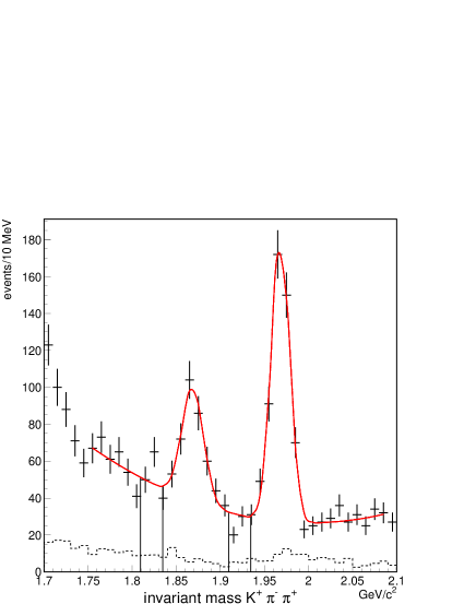
Figure 18: The invariant mass plot of $\mbox{{D}}^{+}\to\mbox{{K}}^{+}\pi^{+}\pi^{-}$ from an earlier FOCUS publication [12]. The Cabibbo suppressed decay $\mbox{{D}}_{s}^{+}\to\mbox{{K}}^{+}\pi^{-}\pi^{+}$ is also visible in this plot.

From this check, it is apparent that genetic programming can yield correct results, even if we don’t understand exactly how. This study also suggests that genetic programming can yield results with greater sensitivity than our standard analysis methods.

6.2 Efficiency comparisons with Monte Carlo

An additional, more challenging, check against the FOCUS Monte Carlo is possible. We can measure the efficiency of the final tree on the Monte Carlo and data. For this study, we look at the ratios of relative efficiency:

$$\frac{\epsilon_{\text{GP-data}}}{\epsilon_{\text{skim-data}}}\,\text{ and }\frac{\epsilon_{\text{GP-MC}}}{\epsilon_{\text{skim-MC}}}$$ (6)

for the Cabibbo favored decay mode which reduces to

$$\frac{Y_{\text{GP-data}}}{Y_{\text{skim-data}}}\,\text{ and }\frac{Y_{\text{GP-MC}}}{Y_{\text{skim-MC}}}\,,$$ (7)

where the various $Y$ values are the yields in Monte Carlo or data with only the skim cuts or the skim cuts and the tree selection applied. In other words, the efficiencies of the tree with respect to the skim on both Monte Carlo and data should be the same if the behavior of the tree is completely modeled by the Monte Carlo. A similar study on doubly Cabibbo suppressed decays is not possible since the yield under the skim cuts is unknown. The results of this study are shown in Table 10.

Table 10: Monte Carlo and data yields $\mbox{{D}}^{+}\to\mbox{{K}}^{-}\pi^{+}\pi^{+}$ for skim cuts only and skim cuts plus the final tree. The values in the final column are the ratios shown in Eq. (6).

Source	Skim yield	GPF yield	Ratio
Data	$253\,190\pm 660$	$62\,440\pm 260$	$24.7\pm 0.1$%
Monte Carlo	$236\,000\pm 500$	$58\,788\pm 245$	$24.9\pm 0.1$%

In this test, the genetic programming tree is very well modeled by the FOCUS Monte Carlo. This was unexpected. We know our Monte Carlo matches the one-dimensional and some two-dimensional distributions of the included variables. But to well model all trees generated by the GPF, the Monte Carlo must correctly model the interrelationships between variables — in this case, a match in 11-dimensional space (one for each terminal in the final tree that is a unique physics variable). Recall that we choose our measurement so that we don’t require that the genetic programming tree perform the same on Monte Carlo and data, only that the tree perform the same on Cabibbo favored and doubly Cabibbo suppressed data. From the very similar efficiencies shown in Table 9, we have additional evidence to believe selection by the genetic programming tree will not be a significant source of systematic error in analyses with such similar final states.

Should close agreement between Monte Carlo and data be required, the fitness function can be redefined to enforce agreement.

6.3 Bias induced by genetic programming optimization

Recall that we attempt to avoid bias by assigning a 0.5% penalty to the fitness for each node in the tree. But, the size of this penalty is arbitrary and is chosen to be small to gently encourage the GPF to produce smaller trees.

To study the possibility that the genetic programming optimization is selecting events based on their specific properties rather than the general properties of all $\mbox{{D}}^{+}\to\mbox{{K}}^{+}\pi^{+}\pi^{-}$ decays, we only optimize on half the events. We can then look at the other half of the events to discover any major problems. (We optimize on even-numbered events, so there is no problem with selecting events from one run period over another, etc.)

In Fig. 19, we show the $\mbox{{D}}^{+}\to\mbox{{K}}^{-}\pi^{+}\pi^{+}$ candidates used and unused in the optimization. While the used portion has a few more events, the difference is statistically insignificant. In Fig. 20, we show the $\mbox{{D}}^{+}\to\mbox{{K}}^{+}\pi^{+}\pi^{-}$ candidates; while there are more signal events in the “used” plot, recall that this region is masked out. It is more instructive to look at the background, since this is susceptible to downward fluctuations. ($B$ is determined from a linear fit with the signal region masked out.) One can see that the background in the two plots is nearly identical. As mentioned above, all fits to doubly Cabibbo suppressed signals use the mass and resolution determined from the Cabibbo favored signals.

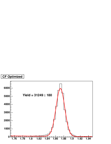
(a) Used candidates

(b) Unused candidates

Figure 19: The $\mbox{{D}}^{+}$ Cabibbo favored decay candidates used (a) in the optimization and those not used (b) as a cross check. The $\mbox{{D}}^{+}$ yields are $31250\pm 180$ and $31200\pm 180$ events respectively.

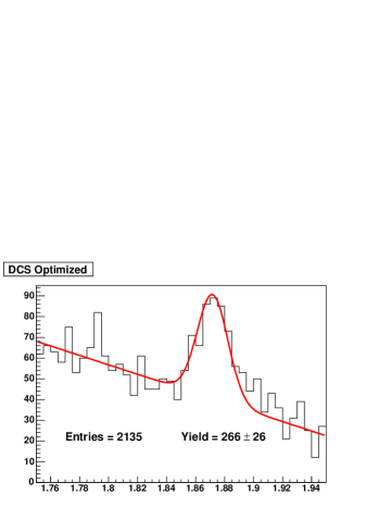
(a) Used candidates

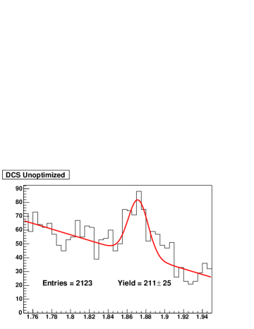
(b) Unused candidates

Figure 20: The $\mbox{{D}}^{+}$ doubly Cabibbo suppressed decay candidates used (a) in the optimization and those not used (b) as a cross check.

To further study possible biases induced by the genetic programming method, analysis of additional runs optimizing on the other half of the events and/or with a different random seed to the GPF would be necessary. Even if there is such a bias, it appears to be small and can easily be incorporated into the systematic error.

6.4 Different Evolutionary Trajectories

In a traditional cut based analysis, one may choose to make measurements with several different sets of cuts. In genetic programming, one analogous method of assessing such variations is to change the trajectory of the evolution. We have studied two ways of doing this. In the first case, we optimize on the odd-numbered rather than even-numbered events. (The initial trees are identical, but their estimated fitnesses differ, causing the evolutionary paths to diverge.) In the second, we change the random number seed at the beginning of the process. We also show the results in the “default” case, but with only 10 rather than 40 generations of evolution.

We then investigate possible differences in three areas. The first observation is the overlap in events between the best tree in the “default” analysis and the best five trees from the “other” analysis. This is shown in Fig. 21. We define two quantities: “false positives,” events which are selected by a given tree but are rejected by the best tree in the default analysis, and “false negatives,” events which are rejected by a given tree but are selected by the best tree. We can see that in the default (even-numbered) case, there are no false positives, but some false negatives. In the other analyses, up to 20% of the events are classified differently by different trees.

Figure 21: The percentage of events classified differently by different trees. For an explanation of the quantities plotted, see the text. The circles show the default optimization, the squares show the results of optimization on odd-numbered events, the triangles ($\blacktriangle$) show the effect of a different random number seed, and the inverted triangles ($\blacktriangledown$) show the effect of stopping the evolution at 10 generations. (Though the five best trees are considered, identical or nearly identical trees cause the number of visible points to be reduced.)

Second, we observe the doubly Cabibbo suppressed signals obtained from the best tree from each of these four different evolutionary trajectories. These are shown in Fig. 22. In all cases, we see a very clear doubly Cabibbo suppressed signal. We can see that the two trajectories optimizing on even-numbered events for 40 generations [plots a) and c)] obtain similar results. Without a large number of different runs with different seeds, it is impossible to say if optimizing on odd vs. events would give generally similar results. However, we can certainly see that we are gaining quite a bit from optimizing for an additional 30 generations. (Compare a) with a $13\sigma$ significance and much better signal-to-background ratio vs. d) with an $11\sigma$ significance.)

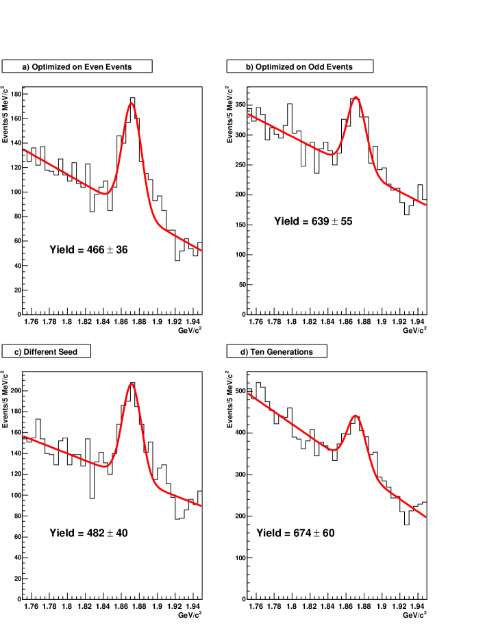
Figure 22: The doubly Cabibbo suppressed signals obtained from four different evolutionary trajectories. a) is the default optimization (with a fitness of 0.123), b) shows the results of optimization on odd-numbered events (fitness: 0.148), c) shows the effect of a different random number seed (fitness: 0.148), and d) shows the effect of stopping the evolution at 10 generations (fitness: 0.194).

Finally, we measure the doubly Cabibbo suppressed branching ratio with the five top trees in each of the four cases. Because, as shown in Table 9, the Monte Carlo corrections to the relative efficiency are small, we simply look at the uncorrected branching ratio, $Y_{\text{DCS}}/Y_{\text{CF}}$. The values for these twenty trees are shown in Fig. 23. As expected, the five trees within each group give nearly identical answers, while some variation is evident between groups. Such a variation, after Monte Carlo efficiency corrections and corrections for expected statistical fluctuations, would form a portion of the systematic error in an analysis using this technique.

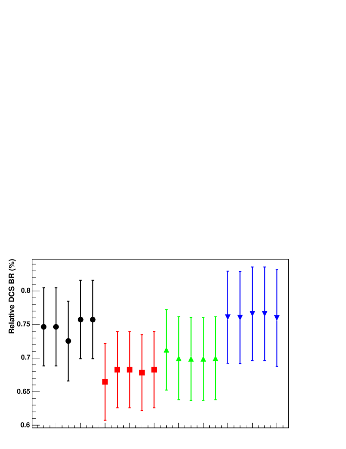
Figure 23: The branching ratio, uncorrected by Monte Carlo, from the five best trees in four runs. The circles show the default optimization, the squares show the results of optimization on odd-numbered events, the triangles show the effect of a different random number seed, and the inverted triangles show the effect of stopping the evolution at 10 generations.

7 Conclusions

We hope we have conveyed an appropriate introduction to genetic programming and how it can be applied in high energy physics analyses. We have demonstrated the use of the technique in separating the doubly Cabibbo suppressed decay $\mbox{{D}}^{+}\to\mbox{{K}}^{+}\pi^{+}\pi^{-}$ from the copious background and shown that this technique can improve upon more traditional analysis techniques. As with any analysis technique, care must be taken to understand the possible systematic errors introduced by the technique. Finally, we have shown that in the FOCUS case, the behavior of Monte Carlo and data is remarkably consistent when the genetic programming method is applied. To our knowledge, this is the first successful application of the genetic programming technique to HEP data.

Other applications for this technique are easy to imagine. Flavor tagging (especially B mesons) has seen several successful implementations of neural networks. Genetic programming may provide another means of tagging. Neutrino closure techniques for semi-leptonic decays may also benefit from such a technique [13, 14].

References

- [1] K. Cranmer, R. S. Bowman, PhysicsGP: A genetic programming approach to event selection, Comput. Phys. Commun. 167 (2005) 165.
- [2] J. R. Koza, Genetic Programming: On the Programming of Computers by Means of Natural Selection, The MIT Press, Cambridge, Massachusetts, 1992.
- [3] W. Banzhaf, P. Nordin, R. E. Keller, F. D. Francone, Genetic Programming—An Introduction: On the Automatic Evolution of Computer Programs and Its Applications, dpunkt.verlag and Morgan Kaufmann Publishers, Inc., San Francisco, California, 1998.
- [4] lil-gp web site, Michigan State University GARARGe group, http://garage.cps.msu.edu/software/lil-gp/lilgp-index.html.
- [5] MSU Genetic Algorithms Research and Applications Group (GARAGe) web site, http://garage.cps.msu.edu/software/software-index.html.
- [6] P. L. Frabetti, et al., Description and performance of the Fermilab E687 spectrometer, Nucl. Instrum. Meth. A320 (1992) 519–547.
- [7] J. M. Link, et al., The target silicon detector for the FOCUS spectrometer, Nucl. Instrum. Meth. A516 (2003) 364–376.
- [8] J. M. Link, et al., Reconstruction of vees, kinks, ’s, and ’s in the FOCUS spectrometer, Nucl. Instrum. Meth. A484 (2002) 174–193.
- [9] J. M. Link, et al., Čerenkov particle identification in FOCUS, Nucl. Instrum. Meth. A484 (2002) 270–286.
- [10] L. Wall, T. Christiansen, R. L. Schwartz, Programming Perl, 2nd Edition, O’Reilly & Associates, Inc., Sebastopol, California, 1996.
- [11] K. Hagiwara, et al., Review of Particle Physics, Phys. Rev. D 66 (2002) 010001.
- [12] J. M. Link, et al., Study of the doubly and singly Cabibbo suppressed decays and , Phys. Lett. B601 (2004) 10–19.
- [13] P. L. Frabetti, et al., Analysis of the decay mode , Phys. Lett. B364 (1995) 127–136.
- [14] J. M. Link, et al., Measurements of the dependence of the and form factors, Phys. Lett. B607 (2005) 233–242.
- [15] ACCRE (Advanced Computing Center for Research & Education, Vanderbilt University) web site, http://www.accre.vanderbilt.edu/accre/.