Measurement of the branching ratios of the $Z^{0}$ into heavy quarks^∗

ABSTRACT

We measure the hadronic branching ratios of the $Z^{0}$ boson into heavy quarks: $R_{b}=\Gamma_{Z^{0}\rightarrow b\overline{b}}/\Gamma_{Z^{0}\rightarrow hadrons}$ and $R_{c}=\Gamma_{Z^{0}\rightarrow c\overline{c}}/\Gamma_{Z^{0}\rightarrow hadrons}$ using a multi-tag technique. The measurement was performed using about 400,000 hadronic $Z^{0}$ events recorded in the SLD experiment at SLAC between 1996 and 1998. The small and stable SLC beam spot and the CCD-based vertex detector were used to reconstruct bottom and charm hadron decay vertices with high efficiency and purity, which enables us to measure most efficiencies from data. We obtain,

$$R_{b}=0.21604\pm 0.00098(stat.)\pm 0.00073(syst.)\mp 0.00012(R_{c})$$

and,

$$R_{c}=0.1744\pm 0.0031(stat.)\pm 0.0020(syst.)\mp 0.0006(R_{b})$$

^∗ Work supported by Department of Energy contract DE-AC03-76SF00515 (SLAC).

1 Introduction

The dominant production of $Z^{0}$ decays, with large statistics, at ${e^{+}e^{-}}$ experiments operating on the $Z^{0}$ peak, provides a unique opportunity for probing electroweak interactions at high precision. The democratic production of all fermion flavors in $Z^{0}$ decays with a clean initial state allows particularly sensitive tests of the Standard Model (SM) through measurements of $R_{b}=\Gamma_{Z^{0}\rightarrow b\overline{b}}/\Gamma_{Z^{0}\rightarrow hadrons}$ and $R_{c}=\Gamma_{Z^{0}\rightarrow c\overline{c}}/\Gamma_{Z^{0}\rightarrow hadrons}$, the heavy quark production fractions in hadronic $Z^{0}$ decays. The $b$ and $c$ quarks are the heaviest charge 1/3 and charge 2/3 quarks, respectively, that are accessible at the $Z^{0}$ energy. The $R_{b}$ measurement has been traditionally a focus of attention as it is not only sensitive to the heavy top quark mass, but also widely regarded as a promising window for detecting new physics through radiative corrections to the ${Z^{0}\rightarrow b\mbox{${\overline{b}}$}}$ coupling. More generally, any unexpected difference in quark coupling of one flavor compared with other flavors could be a vital clue toward a solution to the puzzle of fermion family degeneracy.

To take full advantage of the large $Z^{0}$ decay samples as an effective flavor physics arena, the advance in vertex detector technologies has played a key role for flavor identification. Unprecedented performance in $b$ quark tagging has made it possible to achieve $R_{b}$ measurements [2][3] at below 1% precision. Our previous $R_{b}$ measurement [3] has demonstrated the effectiveness of the combination of high resolution vertexing and the small and stable interaction point at the SLC, which pointed the way for very high purity $b$-tags and led to the reduction of systematic uncertainties for $R_{b}$ measurements in general. In this paper we present an updated $R_{b}$ measurement from SLD using $\sim$2.5 times more statistics than our previous publication and with an upgraded CCD pixel vertex detector, which improves the $b$-tag efficiency to approximately a factor of two higher than $b$-tags used in existing measurements at similar $b$-purity.

The existing measurements of the charm branching ratio $R_{c}$ [4] are considerably less precise than the $R_{b}$ measurements. These determinations of $R_{c}$ rely on a number of methods to identify charm jets that all have certain disadvantages. Exclusive reconstruction of charmed mesons suffers from a small branching fraction and introduces a dependence on the actual value of this branching fraction and on the production fractions of the charm hadrons. Inclusive reconstruction using leptons or slow pions suffer from low purities and again a dependence on branching fractions. Due to the superb performance of the SLD vertex detector we are able to introduce an inclusive charm tag, based on lifetime information in a similar way as the $b$ tag, which combines high efficiency with good purity. Moreover, the tagging efficiencies are measured from data and result in a minimal reliance on Monte Carlo simulation and a small systematic uncertainty. This leads to a new determination of $R_{c}$ with much improved overall precision than the existing measurements.

2 Apparatus and Hadronic Event Selection

This analysis is based on approximately 400,000 hadronic events produced in ${e^{+}e^{-}}$ annihilations at a mean center-of-mass energy of $\sqrt{s}=91.28$ GeV at the SLAC Linear Collider (SLC), and recorded in the SLC Large Detector (SLD) between 1996 and 1998. A general description of the SLD can be found elsewhere [5]. The trigger and initial selection criteria for hadronic $Z^{0}$ decays are described in Ref. [6]. The Central Drift Chamber (CDC) [7] and the upgraded Vertex Detector (VXD3) [8], inside a uniform axial magnetic field of 0.6T, provide the momentum measurements of charged tracks and precision vertex information near the interaction point (IP), which are central to this analysis. The energies of clusters measured in the Liquid Argon Calorimeter [9] are used for event selection and calculation of the event thrust axis.

SLD uses a coordinate system with the $z$-axis parallel to the beam direction and $x$ and $y$ respectively are the horizontal and vertical coordinates perpendicular to the $z$-axis. The polar angle $\theta$ is measured with respect to the $z$-axis and the azimuthal angle $\phi$ is the angle with the $x$-axis in the $xy$ plane.

The CDC and VXD3 give a combined momentum resolution of $\sigma_{p_{\perp}}/p_{\perp}$ = $0.01\oplus 0.0026p_{\perp}$, where $p_{\perp}$ is the track momentum transverse to the beam axis in ${\mathrm{\,Ge\kern-1.00006ptV\!/}c}$. The VXD3 consists of 3 barrels of Charged Coupled Devices (CCD) at radii of 2.7, 3.8 and 4.8 centimeters from the beam line, with 3-hit solid angle coverage up to $|\cos\theta|$=0.85. The CCD pixels are cubic active volumes of 20$\,\mu\rm m$ on each side, which provide precise 3D spatial hits. This high granularity in 3D space enable our track finding algorithm to limit the hit mis-assignment rate to only 0.2%. The spatial resolution on the hit cluster centroid achieved after a track based CCD alignment [10] is $\sim$4$\,\mu\rm m$ in both azimuthal and $z$ directions. The resultant tracking resolution for high momentum tracks, as measured from the miss distances of two tracks near the IP in ${Z^{0}\rightarrow\mu^{+}\mu^{-}}$ events, is 7.7$\,\mu\rm m$ in $r\phi$ and 9.6$\,\mu\rm m$ in $rz$. The multiple scattering contribution to the track impact parameter resolution can be approximately expressed as $\frac{33}{p\sin^{3/2}\theta}$ $\,\mu\rm m$. These numbers are roughly a factor of two better than a typical vertex detector at LEP. This resolution advantage combined with the small and stable SLC IP information is crucial in establishing the feasibility of the measurement techniques, in particular for the case of the inclusive charm tagging for the $R_{c}$ measurement.

For the purpose of estimating the efficiencies and purities of the event selection and flavor tagging procedures, we use a detailed Monte Carlo (MC) simulation of the detector. The JETSET 7.4 [11] event generator is used, with parameter values tuned to hadronic ${e^{+}e^{-}}$ annihilation data [12], combined with a simulation of the SLD based on GEANT 3.21 [13]. The simulations of heavy hadron production and charm decays are described in [6]. The $B$ decay simulation is adapted from the CLEO QQ MC with additional tuning by SLD (see appendix B of [14]) to match a wider range of $\Upsilon(4S)$ $B$ decay data.

For the hadronic event selection, we use a set of well-measured tracks, consistent with originating from within the beam pipe radius of 2.5 cm. The selected events have at least 7 tracks with $p_{\perp}>$0.2${\mathrm{\,Ge\kern-1.00006ptV\!/}c}$ and within 5$\rm\,cm$ from the interaction point along the beam axis. There are at least 3 tracks with two or more VXD hits. The event visible energy $E_{vis}$, calculated from charged tracks with the charged pion mass assigned, must be at least 18 GeV. To ensure the events are well contained within the detector fiducial volume, we require the thrust-axis polar angle w.r.t. the beamline, $\theta_{T}$, calculated using calorimeter clusters, to be within $|\cos\theta_{T}|<$0.7. We only include events with $\leq$3 jets for the analysis, where the jets are reconstructed from tracks using the JADE algorithm [15] with $y_{cut}=0.02$. This last requirement is to reject higher jet multiplicity events where the division of events into two hemispheres is no longer reliable for partitioning the events with one heavy hadron in each hemisphere.

The selected event sample contains 191,770 events from the 1997-98 runs and 29,996 events from the 1996 run. We analyze the two data samples separately because the small 1996 sample, recorded during the early VXD3 commissioning period, has a lower overall VXD hit efficiency due to electronics problems and some radiation damage. This effect was not present in the 97-98 period when the VXD3 ran at $\sim$10 degrees colder and the operation of the electronics was much more stable.

The estimated background in the hadronic event sample is negligible. The Monte Carlo ${Z^{0}\rightarrow hadrons}$ event statistics used in the analysis have MC:data event ratios of 4:1, 15:1, and 22:1 for light flavor quarks ($uds$), ${c\mbox{${\overline{c}}$}}$, and $b\mbox{${\overline{b}}$}$ events, respectively.

3 Heavy Flavor Tagging

Decays of $Z^{0}$ bosons into charm and bottom quarks can be distinguished from those into light flavors ($u$,$d$ and $s$) by searching for the heavy hadron decay vertices displaced from the event interaction point (IP). Because they are produced with high energy and have long lifetimes, heavy hadrons generally travel distances of millimeters before decaying. In a jet from a light quark the tracks will appear to come from one point in space, the event IP. In a charm jet some of the tracks may not point back to the IP, and if the charmed hadron decays into more than one charged particle there will be a secondary vertex (SV) in addition to the IP. Bottom jets will also exhibit secondary vertices, and if there are sufficient particles produced at the $b$ and $c$ decay points it is possible to find more than one displaced vertex. The reconstructed secondary vertices and their associated kinematic properties serve as the primary basis for flavor tagging for both $b\mbox{${\overline{b}}$}$ and ${c\mbox{${\overline{c}}$}}$ events in this analysis.

3.1 IP Reconstruction

To search for displaced vertices the position of the IP must be precisely known. In each event the position of the IP in the plane transverse to the beam axis is determined by fitting all tracks that are compatible with coming from the IP to a common vertex. Because the SLC luminous region is small and stable in the $xy$ plane, sets of 30 time sequential hadronic events are averaged to obtain a more precise determination of the $xy$ IP position (details in appendix A of [14]). The $xy$ IP resolution is measured from the impact parameter distributions of ${Z^{0}\rightarrow\mu^{+}\mu^{-}}$ events, deconvolved from the track impact parameter resolution measured from the two track miss distance, to obtain an IP resolution of 3.2$\,\mu\rm m$.

Because the SLC luminous region is larger in $z$ (700 $\mu$m), the $z$ position of the IP must be found event-by-event. Tracks with VXD hits are extrapolated to their point of closest approach (POCA) in $xy$ to the precisely determined transverse IP position. Tracks with impact parameters of more than 500$\,\mu\rm m$ or 3 times the error ($\sigma$) from the IP are excluded, and the $z$ position of the IP is taken from the median $z$ at POCA of the remaining tracks. The resolution of this method is found from the Monte Carlo simulation to be 10/11/17 $\,\mu\rm m$ for $uds$/${c\mbox{${\overline{c}}$}}$/$b\mbox{${\overline{b}}$}$ events.

3.2 Secondary Vertex Reconstruction

Secondary vertices are found using a topological algorithm [16]. This method searches for space points of large track density in 3 dimensions. Each track is parameterized by a Gaussian probability density tube $f(\vec{r})$ with a width equal to the uncertainty in the track position at its POCA to the IP, $\vec{r}_{0}$:

$$f(\vec{r})=\exp\left\{-\frac{1}{2}\left[\left(\frac{x-(x_{0}+y^{2}\kappa)}{\sigma_{1}}\right)^{2}+\left(\frac{z-(z_{0}+y\tan\lambda)}{\sigma_{2}}\right)^{2}\right]\right\}.$$ (1)

The first term is a parabolic approximation to the track’s circular trajectory in the $xy$ plane, where $\kappa$ is a function of the track’s charge and transverse momentum and of the SLD magnetic field. The second term represents the linear trajectory of the track in the $rz$ plane, where $\lambda$ is the track dip angle from the vertical. The $\sigma$ parameters are the uncertainties in the track positions after extrapolation to $\vec{r}_{0}$ for the two projections. The function $f_{i}(\vec{r})$ is formed for each track $i$ under consideration and used to construct the vertex probability function $V(\vec{r})$. Also included is $f_{0}(\vec{r})$, a $7\times 7\times 20$ $\mu$m $(x\times y\times z)$ Gaussian ellipsoid centered at the IP position.

$$V(\vec{r})=\sum_{i}f_{i}(\vec{r})-\frac{\sum_{i}f_{i}^{2}(\vec{r})}{\sum_{i}f_{i}(\vec{r})}$$ (2)

Secondary vertices are found by searching for local maxima in $V(\vec{r})$ that are well-separated from the peak at the IP position. The tracks whose density functions contribute to such a local maximum are then identified as originating from a secondary vertex (SV).

A loose set of cuts is applied to tracks used for secondary vertex reconstruction. Tracks are required to have $\geq 2$ VXD hits and $p_{\perp}>250$${\mathrm{\,Me\kern-1.00006ptV\!/}c}$. Tracks with 3D impact parameter $>3$ mm or consistent with originating from a $K_{s}^{0}$ or $\Lambda$ decay, or $\gamma$ conversion are also removed. Each event is divided into two hemispheres using the thrust axis, and the vertexing procedure is performed in each using only the tracks in that hemisphere. The identified vertices are required to be within 2.3 cm of the center of the beam pipe to remove false vertices from interactions with the detector material. A cut on the secondary vertex invariant mass $M$ of $|M-M_{K^{0}_{S}}|<0.015$ GeV/$c^{2}$ removes any $K^{0}_{S}$ decays that survived the track cuts. The remaining vertices are then passed through a neural network [17] to improve the background rejection further. The input variables are the flight distance from the IP to the vertex ($D$), that distance normalized by its error ($D/\sigma_{D}$), and the angle $\phi_{PD}$ between the flight direction $\vec{D}$ and the total momentum vector of the vertex $\vec{P}$. These quantities are shown in Figure 1, along with the output value of the neural network ($y_{vtx}$). A good vertex in simulation is defined as one which contains only tracks from heavy hadron decays, with no tracks originating from the IP, strange particle decays, or other sources. Vertices with $y_{vtx}>0.7$ are retained. At least one secondary vertex passing this cut is found in 72.7% of bottom, 28.2% of charm, and 0.41% of light quark event hemispheres in the Monte Carlo. Around 16% of the hemispheres in $b$ events have more than one selected secondary vertex.

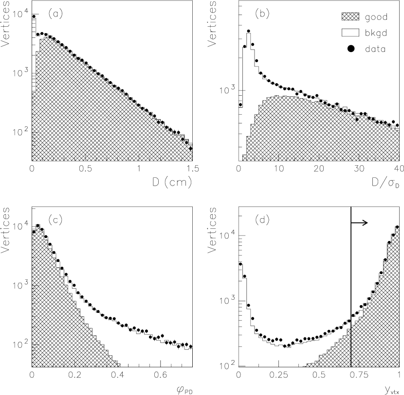
Figure 1: Distributions of seed vertex selection variables: (a) distance from IP $D$, (b) normalized distance from IP $D/\sigma_{D}$, (c) angle between flight direction and vertex momentum $\phi_{PD}$, (d) neural network output $y_{vtx}$. A good vertex contains only heavy hadron decay tracks. The arrow indicates the accepted region.

3.3 Track Attachment

Due to the cascade nature of $b$ hadron decays, tracks from the heavy hadron may not all originate from the same space point. Therefore, a process of attaching tracks to the secondary vertex (SV) has been developed to recover this information using a second neural network. The first four inputs are defined at the point of closest approach of the track to the axis joining the secondary vertex to the IP. They are the transverse distance from the track to that axis ($T$), the distance from the IP along that axis to the POCA ($L$), that distance divided by the flight distance of the SV from the IP ($L/D$), and the angle of the track to the IP-SV axis ($\alpha$). The last input is the 3D impact parameter of the track to the IP normalized by its error ($b/\sigma_{b}$). These quantities are shown schematically in Figure 2. The distributions are shown in Figure 3, along with the neural network output value ($y_{trk}$). The network is trained to accept only tracks which come from a $b$ or $c$ hadron decay, and to reject tracks from the IP or from strange particle decays or detector interaction products. If more than one secondary vertex was found in the hemisphere the attachment procedure is tried for each track-SV combination. Tracks with $y_{trk}>0.6$ are added to the list of secondary vertex tracks. This value is chosen to minimize the number of fake tracks being attached to charm vertices, which than could mimic a $b$ decay.

Figure 2: Schematic illustration of the quantities used in the track-attachment procedure described in the text (not to scale).

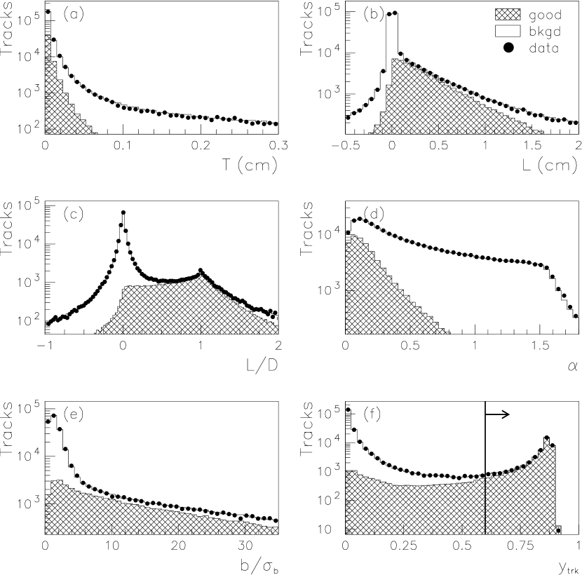
Figure 3: Distributions of the cascade track selection variables described in the text: (a) $T$, (b) $L$, (c) $L/D$, (d) $\alpha$, (e) $b/\sigma_{b}$, (f) neural network output $y_{trk}$. A good track is one which originates from a heavy hadron decay. The arrow indicates the accepted region.

3.4 Flavor Discrimination

At this point, for each hemisphere there is a list of selected tracks. For hemispheres with no selected secondary vertices the list is empty, otherwise it includes the tracks in the secondary vertices and any cascade tracks which have been attached. From this list several signatures can be computed to discriminate between bottom/charm/light event hemispheres. These are the invariant mass of the selected tracks corrected for missing $P_{t}$ ($M_{hem}$), the total momentum sum of the selected tracks ($P_{hem}$), the distance from the IP to the vertex obtained by fitting all of the selected tracks ($D_{hem}$), and the total number of selected tracks ($N_{hem}$).

The four signatures given above are used as inputs for a neural network trained to distinguish hemispheres in bottom/charm/light events. The four inputs and the neural network output $y_{hem}$ are shown in Figure 4. The $P_{t}$ corrected mass $M_{hem}$ [3], is a particularly powerful discriminator to separate bottom and charm. For a detector with high precision vertexing capability, decay vertices from $b$ and $c$ hadrons can both be very distinctively separated from the IP at high efficiency. The large $b$ hadron mass is then the key kinematic information to allow separation of $b\mbox{${\overline{b}}$}$ and ${c\mbox{${\overline{c}}$}}$ with high purity, which is crucial for these precision measurements. The raw vertex mass from the selected charged tracks can already give high purity $b$ tags once requiring mass above the charm threshold, but many $b$ decays with missing neutrals have an apparent low vertex mass. With the secondary vertex and PV positions very precisely measured at SLD, the $b$ hadron flight direction can be derived to compare with the vector sum of the selected secondary track momenta to estimate the missing $P_{t}$ with respect to the $b$ hadron flight direction. A corrected vertex mass is then calculated to compensate for the derived minimal missing mass, taking into account the vertex position errors:

$$M_{hem}=\sqrt{m_{c}^{2}+P_{t}^{2}}+|P_{t}|$$ (3)

where $m_{c}$ is the invariant mass of the tracks attached to the secondary vertex in the hemisphere.

Vertices in $c$ quark jets, near the charm mass threshold typically have small missing $P_{t}$, while many $b$ vertices near the charm mass threshold receive a large missing $P_{t}$ correction to become well separated from ${c\mbox{${\overline{c}}$}}$ events. The missing particles for the low mass $b$ vertices generally lead to a lower apparent momentum calculated from the visible charged tracks so that the correlation between $P_{hem}$ and $M_{hem}$ presents another effective handle to further improve the flavor separation, as shown in (f) and (g) of Figure 4, comparing $c$ and $b$ jets.

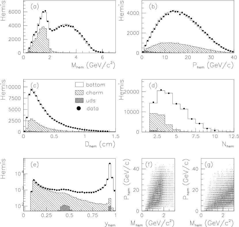
Figure 4: Distributions of flavor discrimination variables: (a) $M_{hem}$, (b) $P_{hem}$, (c) $D_{hem}$, (d) $N_{hem}$, (e) neural network output $y_{hem}$, (f) $P_{hem}$ vs. $M_{hem}$ correlation for $c$ jets (g) same for $b$ jets.

The flavor selection neural network is trained to put charm event hemispheres near $y_{hem}=0$, bottom event hemispheres near $y_{hem}=1$, and light-flavor background near $y_{hem}=0.5$. This allows a simple selection of charm (bottom) event hemispheres by specifying an upper (lower) limit for the output value $y_{hem}$. Figure 5 shows the ranges of purity vs. efficiency which can be obtained for charm and bottom event hemisphere tagging by adjusting this one cut. As can be seen in Figures 1 and 4, the inputs used for the neural networks at various stages of the $y_{hem}$ tag construction are in reasonable agreement between data and MC. However, an exact agreement is not essential as the main tagging efficiencies will be measured directly from the data.

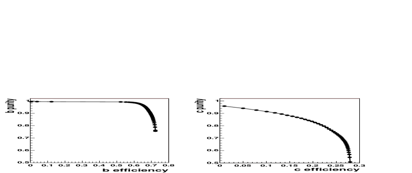
Figure 5: Purity vs. efficiency for hemispheres in (a) charm and (b) bottom events, as the selection neural network cut is varied.

4 Measurement Method and Results

Each event is divided into two hemispheres by the plane perpendicular to the thrust axis. Both measurements apply flavor tags on each hemisphere separately to derive $R_{b}$ and $R_{c}$, and measure the major tagging efficiencies from data simultaneously.

4.1 $R_{b}$ measurement

For the $R_{b}$ measurement, we define a single $b$-tag with $y_{hem}>$0.75 and apply the classical double tag method as in our previous measurement [3]. By counting the fraction of tagged hemispheres, $F_{s}$, and the fraction of events with both hemispheres tagged, $F_{d}$, we can measure $R_{b}$ by iteratively solving the following equations:

$$F_{s} = \mbox{${\epsilon_{b}}$}R_{b}+\mbox{${\epsilon_{c}}$}R_{c}+\mbox{${\epsilon_{uds}}$}(1-R_{b}-R_{c}),$$

$$F_{d} = C_{b}\mbox{${\epsilon_{b}^{2}}$}R_{b}+C_{c}\mbox{${\epsilon_{c}^{2}}$}R_{c}+\mbox{${\epsilon_{uds}^{2}}$}(1-R_{b}-R_{c}).$$ (4)

where $\mbox{${\epsilon_{uds}}$},\mbox{${\epsilon_{c}}$}$ and ${\epsilon_{b}}$ are the hemisphere tagging efficiencies for $uds$, $c$ and $b$ hemispheres, respectively, and $C_{q}=\frac{\epsilon_{q}^{double}}{\epsilon_{q}^{2}}$, are the hemisphere tag correlations for $b$ and $c$ events. We ignore the correlation for $uds$ events since we expect 0.23 double tagged events. A Standard Model value of $R_{c}$=0.1723 is assumed. The dependence on MC simulation is greatly reduced by measuring ${\epsilon_{b}}$ from data, while only the small ${\epsilon_{c}}$,${\epsilon_{uds}}$ and correlations are estimated from MC. The measurement results and estimated MC parameters are tabulated in Table 1 for the 96 and 97-98 data samples. The errors are statistical only for both measured and MC parameters. The $R_{b}$ result has been corrected by $-0.00149$ for hadronic event selection bias and by $+0.00024$ for $Z\gamma$ interference effect.

	96			97-98
$R_{b}$	0.21432	$\pm$	0.00289	0.21624	$\pm$	0.00104
${\epsilon_{b}}$(data)(%)	56.63	$\pm$	0.67	62.01	$\pm$	0.24
${\epsilon_{b}}$(MC)(%)	56.91	$\pm$	0.08	61.78	$\pm$	0.03
$\Pi_{b}$ (%)	97.8	$\pm$	0.4	97.9	$\pm$	0.1
${\epsilon_{c}}$(MC)(%)	1.24	$\pm$	0.02	1.19	$\pm$	0.01
${\epsilon_{uds}}$(MC)(%)	0.113	$\pm$	0.006	0.134	$\pm$	0.003
$C_{b}-1$(MC)	0.0067	$\pm$	0.0015	-0.00012	$\pm$	0.00049
$C_{c}-1$(MC)	0.16	$\pm$	0.26	0.30	$\pm$	0.12
N events	29996			191770
N single tag	3315			20738
N double tag	2091			16048

Table 1: $R_{b}$ result and tagging performance parameters. $\Pi_{b}$ is the hemisphere $b$-tag purity. All errors are statistical only.

4.2 $R_{c}$ measurement

Unlike the case of the $R_{b}$ measurement where the single $y_{hem}>0.75$ tag has already collected $b$ hemispheres with both high efficiency and high purity, the charm events are more spread out in the $y_{hem}$ distribution. Since the number of double tagged events is very sensitive to the tag efficiency, the lower efficiency for charm tagging makes the use of different tags with quite different purities more profitable. We therefore use a multi-tag approach for the $R_{c}$ measurement.

We divide hemispheres with a secondary vertex into four tag categories, depending on the output value of the neural network, $y_{hem}$. A $b$ tag (tag 4) with $y_{hem}>0.75$, a charm tag (tag 1) with $y_{hem}<0.3$, a low-purity $b$-tag (tag 3) with $0.5<y_{hem}<0.75$ and a low-purity charm tag (tag 2) with $0.3<y_{hem}<0.5$. Hemispheres without a secondary vertex are classified in the tag 0 category. In total we have 15 different event categories $N_{ij},i\leq j\leq 4$ for the different tag combinations with a predicted fraction of the number of events $G_{ij}$ :

$$G_{ij}=\kappa[\epsilon_{b}^{i}\epsilon_{b}^{j}C_{b}^{ij}R_{b}+\epsilon_{c}^{i}\epsilon_{c}^{j}C_{c}^{ij}R_{c}+\epsilon_{uds}^{i}\epsilon_{uds}^{j}C_{uds}^{ij}(1-R_{b}-R_{c})]$$ (5)

with $\kappa=1$ for $i=j$ and 2 for $i\neq j$. $\epsilon_{q}^{i}$ is the efficiency for quark $q$ to give a tag $i$. $C^{ij}$ is the tag correlation between tag $i$ and tag $j$ similarly defined as in the $R_{b}$ case. Since $N_{00}$ is determined by the total number of events and the other event counts, we have 14 independent equations for the event fractions $F_{ij}=N_{ij}/N_{\mbox{total}}$.

A small number of $uds$ events produce a secondary vertex. This has two reasons. The first is gluon splitting to $b\overline{b}$ and $c\overline{c}$. The result is a real heavy quark of which the decay is well modeled in our simulation. These events mainly populate the high purity $b$ and $c$ tag categories and the errors on the measured rates dominate the systematic uncertainty assigned to this effect. The other source is incorrect reconstruction in our detector. These events typically cluster around $y_{hem}=0.5$. This is less well modeled, and in the next section we estimate the error on the rate predicted by our simulation to be 10%. The $N_{02}$ and $N_{03}$ categories contain most of these events. To avoid a bias from these low purity bins, we de-weight them by taking as the error on the event fraction, $\sigma_{F_{ij}}$, the binomial error on the bin contents and the systematic effect from varying the non-gluon splitting $uds$ efficiency by 10%, added in quadrature.

We minimize

$$\chi^{2}=\Sigma_{i,j,i\leq j}(F_{ij}-G_{ij})^{2}/(\sigma_{F_{ij}})^{2}$$ (6)

as a function of the following 9 parameters: $R_{b}$, $R_{c}$, $\epsilon_{b}^{j}$ ($j=1,4$) and $\epsilon_{c}^{j}$ ($j=1,3$). The $c$-quark efficiency for the $b$-tag, $\epsilon_{c}^{4}$, all light quark efficiencies, $\epsilon_{uds}^{j}$ $(j=1,4)$ and the hemisphere correlations $C^{ij}_{q}$ are taken from Monte Carlo. Only a few of the correlations are different from 1 in a statistically significant way. The others are set to 1.

The $R_{c}$ fit results are summarized in Table 2. The $R_{c}$ values have been corrected by $-0.0004$ for $Z\gamma$ interference, the event selection bias is zero in simulation. The $R_{c}$ values are given at a central $R_{b}$ value of $0.2157$. The measured value of $R_{b}$ agrees with the determination from the $R_{b}$ measurement. There is a good agreement between the efficiencies in Monte Carlo and Data in the high purity tags 1 and 4. The efficiency for the lower purity tags 2 and 3 for charm is higher in Monte Carlo than in the 97-98 data sample. The Monte Carlo efficiency is quite sensitive to physics parameters like the charmed hadron production fractions, their decay multiplicities and their lifetimes. The measured value of the efficiency can be reproduced in the Monte Carlo, by varying some of these parameters within their allowed range as is done in the study of systematic uncertainties. Since we extract the efficiencies from the data, the measured value of $R_{c}$ is insensitive to these variations.

	96		97-98
	data	MC	data	MC
$R_{c}$	$0.1678\pm 0.0091$		$0.1752\pm 0.0033$
$\epsilon^{1}_{b}$ (%)	$2.22\pm 0.18$	$2.01$	$2.52\pm 0.07$	$2.36$
$\epsilon^{1}_{c}$ (%)	$16.09\pm 0.90$	$15.75$	$17.95\pm 0.36$	$18.56$
$\epsilon^{1}_{uds}$ (%)		$0.088$		$0.063$
$\epsilon^{2}_{b}$ (%)	$2.83\pm 0.20$	$2.56$	$2.97\pm 0.07$	$3.00$
$\epsilon^{2}_{c}$ (%)	$4.93\pm 0.36$	$5.05$	$5.02\pm 0.13$	$5.72$
$\epsilon^{2}_{uds}$ (%)		$0.117$		$0.124$
$\epsilon^{3}_{b}$ (%)	$4.68\pm 0.24$	$4.40$	$5.10\pm 0.09$	$4.98$
$\epsilon^{3}_{c}$ (%)	$2.46\pm 0.27$	$2.59$	$2.23\pm 0.10$	$2.87$
$\epsilon^{3}_{uds}$ (%)		$0.150$		$0.140$
$\epsilon^{4}_{b}$ (%)	$56.8\pm 0.64$	$56.9$	$62.18\pm 0.23$	$61.78$
$\epsilon^{4}_{c}$ (%)		$1.23$		$1.19$
$\epsilon^{4}_{uds}$ (%)		$0.113$		$0.134$
$C_{c}^{11}-1$		-0.0068		0.012
$C_{b}^{14}-1$		0.0032		0.0011
$C_{b}^{34}-1$		0.0064		-0.0015
$C_{b}^{44}-1$		0.0067		-0.00012
other $C_{q}^{ij}-1$		0		0
$\chi^{2}/d.o.f.$	$6.66/5$		$7.05/5$

Table 2: $R_{c}$ results and tagging performance parameters. The errors on the MC efficiencies are small compared to systematic uncertainties and therefore omitted

5 Systematic Errors and Cross-checks

The systematic uncertainties on $R_{b}$ and $R_{c}$ result from a combination of detector related effects and physics uncertainties in the simulation which affect our estimates of ${\epsilon_{c}}$, ${\epsilon_{uds}}$ and $C_{q}$ in the case of $R_{b}$ and $\epsilon_{4}^{c}$, $\epsilon^{uds}_{i}$ and all correlations for $R_{c}$. These systematic uncertainties are listed in Table 7 for the combined results for 96 and 97-98 data, which are analyzed separately initially.

5.1 Hemisphere correlation cross check

With the statistical precision down to the $<$0.5% level for $R_{b}$ and the $<$2% level for $R_{c}$, the systematic uncertainties of the small subtle effects of hemisphere tag correlation become important. As the correlations have a variety of origins and the evaluation of their uncertainties will be spread over many subsections to follow, we will first discuss the correlation sources to establish an understanding of the magnitude of their effects. Primarily as a cross check to constrain possible missing systematic sources for the hemisphere correlations, we decompose the efficiency correlation of the $b$ and $c$ tags into a set of approximately independent components which represent the major known sources of correlation between the two hemispheres in the $b\mbox{${\overline{b}}$}$ and ${c\mbox{${\overline{c}}$}}$ MC events.

To focus on understanding the physics sources, we use the large uniform 97-98 MC sample without tracking efficiency and resolution corrections, to avoid the statistical fluctuations introduced by the tracking corrections. The overall tracking systematic effects will be evaluated separately in section 5.3.1. For the $R_{c}$ measurement, there are many correlations between the different tags. We present a representative $c$-tag of $y_{hem}<0.4$, for similar set of effects as for the $b$-tag. For this study we need to identify the relevant kinematic and geometric variables to see how the tagging efficiencies depend on them and how the two hemispheres correlate on these variables.

The primary vertex (PV) shared between the two hemispheres is an obvious source of correlation. A misreconstructed PV results in a negative correlation if the displacement is along the thrust axis. Displacement of the PV transverse to the thrust axis would tend to positively correlate the two hemispheres. The small and stable SLD IP in the $xy$ view is an average beam position over many events which greatly reduces the chance of large PV displacement in $xy$, and restricts the remaining effect to be only through the IP $z$ coordinate, which is reconstructed event by event. The total PV effect is studied by simply comparing results using the reconstructed PV and using the MC truth PV.

Another major source is geometric correlations. The two hemispheres are exactly back to back by definition. Due the cylindrical geometry of the detector, larger $|\cos\theta|$ typically means more multiple scattering, worse tracking efficiency and resolution, worse radial alignment etc. This will affect the hemisphere at $\cos\theta$ and the opposite hemisphere at $-\cos\theta$ in the same way. We calculate the tagging efficiency in bins of the hemisphere axis $\cos\theta$ bin and construct a function $\epsilon(\cos\theta)$. The $\cos\theta$ correlation component can then be estimated from

$$C=\sum_{i}\epsilon(\cos\theta_{i})\cdot\epsilon(-\cos\theta_{i})\,f(\cos\theta_{i})/\overline{\epsilon}^{2}$$

where $i$ is the index of the $\cos\theta$ bin, $f$ is the fraction of all events in bin $i$ and $\overline{\epsilon}$ is the average tagging efficiency of all hemispheres.

Although the cylindrical geometry of the detector ensures uniformity at first order in azimuth, local performance variation of detector elements can still introduce an effect. Similar to the $\theta$ component analysis, the $\phi$ component is estimated from

$$C=\sum_{i}\epsilon_{forward}(\phi_{i})\cdot\epsilon_{backward}(\phi_{i}+\pi)\,f(\phi_{i})/\overline{\epsilon}^{2}$$

where the efficiency parameterization is done for forward ($+z$) and backward ($-z$) hemispheres separately.

Tagging correlation due to variation of detector performance in time also needs to be addressed. This is in fact the primary reason that the 97-98 data and 96 data are analyzed separately. There is a significant VXD3 performance variation during the 96 run, and the Monte Carlo simulation reproduces these time dependent effects in detail. The time dependent component is estimated from

$$C=\sum_{i}\epsilon^{2}(R_{i})\,f(R_{i})/\overline{\epsilon}^{2}$$

where $R_{i}$ is a group of runs adjacent in time, $f(R_{i})$ is the fraction of all events in this group of runs.

The $b/c$-tag efficiencies have a significant dependence on the heavy hadron momentum ($P_{H}$) and its angle to the hemisphere axis ($\xi$). There are various causes, such as gluon radiation, which can result in correlations of the heavy hadron momenta and angular distributions. For the momentum correlation component, we parameterize the hemisphere tagging efficiency in a 2D grid of $\epsilon(P_{H},\xi)$ then sum over all events $i$ for the correlation for hemispheres 1 and 2:

$$C=\sum_{i}\epsilon(P^{i}_{H1},\xi^{i}_{1})\cdot\epsilon(P^{i}_{H2},\xi^{i}_{2})/\overline{\epsilon}^{2}$$

This component is only evaluated for the normal cases where two heavy quarks are in opposite hemispheres. The joint effect of the heavy hadron momentum and thrust angle is $\sim$20% larger than the effect from momentum alone.

For the extreme case of hard gluon radiation, with two heavy quarks recoiling into the same hemisphere opposite the hard gluon, we simply calculate the effect if including and excluding these events in the overall sample. The magnitudes of the various components and their sum compared with the overall correlations calculated from the MC hemisphere and double tag rates are shown in Table 3.

Component	$(C_{b-tag}-1)\times 10^{5}$		$(C_{c-tag}-1)\times 10^{5}$
	97-98	96	97-98	96
Primary vertex	$+46$	$+13$	$-480$	$-640$
Geometrical correlation $\theta$	$+49$	$+60$	$+120$	$-120$
Geometrical correlation $\phi$	$-4$	$+212$	$-10$	$+170$
Time dependence	$11$	$+434$	$+40$	$+870$
$B/D$ momentum and thrust angle	$+107$	$+95$	$+820$	$+760$
Hard gluon radiation	$-37$	$-23$	$+510$	$+410$
Component sum	$+170$	$+670$	$+1000$	$+1450$
MC overall correlation	$+42$	$+891$	$+420$	$+1510$
MC statistical error	$\pm 47$	$\pm 113$	$\pm 390$	$\pm 1210$
discrepancy	$+128$	$-121$	$+580$	$-60$

Table 3: Hemisphere correlation component check results for $b$-tag and $c$-tag.

An important observation is that the magnitude of all components are small, which is especially true for the $b$-tag. The change in the value of the correlation $C$ translates to the fractional error of $R_{b}$ and $R_{c}$. So effects at typically 0.1% (1%) or less for the $b$($c$)-tag can be compared with the $R_{b}$ ($R_{c}$) statistical error of $\sim$0.5% (2%). This illustrates the importance of the large tagging efficiency in driving a much smaller correlation and reducing sensitivity to correlation uncertainties, which is even apparent when comparing the $b$-tag with the $c$-tag. In the limit of 100% tagging efficiency, the correlation becomes irrelevant.

The 96 samples are not large enough to draw detailed conclusions given the large MC statistical error, but the difference of the overall correlation between 96 and 97-98 is well explained by the known time and $\phi$ dependent effects in 96. For the more statistically significant test with the 97-98 sample, there is a noticeable discrepancy between the $b$-tag component sum and the MC overall correlation. Although at least part of the discrepancy could be statistical for this approximate cross check, we take half of discrepancies from the 97-98 analysis for both the $b$-tag and $c$-tag as an additional systematic error associated with possible missing sources.

5.2 Physics systematics

The physics systematic errors are mostly assigned by reweighting the nominal simulated distributions to an alternative set of distributions which correspond to the world average measurements and uncertainties of the underlying MC physics parameters [18].

5.2.1 ${g\rightarrow{Q\overline{Q}}}$ effect

The ${g\rightarrow{b\overline{b}}}$ and ${g\rightarrow{c\overline{c}}}$ production rates are varied according to the experimental averages [18]. These measurement rates are significantly higher than the default JETSET MC as shown in Table 4.

	${g\rightarrow{c\overline{c}}}$ (%)	${g\rightarrow{b\overline{b}}}$ (%)
LEPEWWG standard	2.96$\pm$0.38	0.254$\pm$0.051
JETSET	1.357	0.142

Table 4: The world average measurements of ${g\rightarrow{Q\overline{Q}}}$ compared to the predictions of the JETSET generator.

The main sensitivity to the gluon splitting uncertainties is through the $uds$ tagging efficiencies. Its effect on charm background under the $b$-tag is also noticeable. In the case of the $R_{b}$ measurement, we can see in detail in Fig. 6 how ${g\rightarrow{Q\overline{Q}}}$ affects the systematic uncertainty on $R_{b}$ as a function of $y_{hem}$ cut.

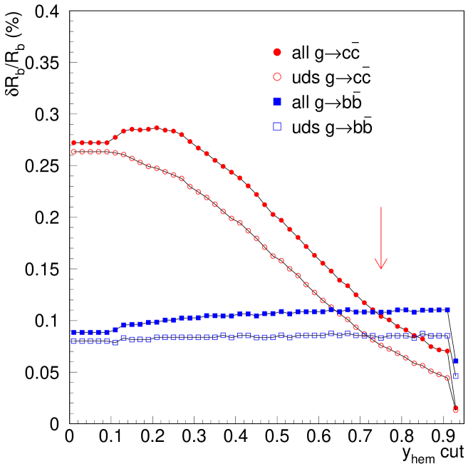
Figure 6: Components of the $R_{b}$ systematic error as a function of the flavor separation $y_{hem}$ cut for the various ${g\rightarrow{Q\overline{Q}}}$ processes.

5.2.2 $uds$ physics modeling

Among the fake $uds$ tags, a significant fraction involve $K^{0}_{s}$ and $\Lambda$ decay product. The MC generator level $K^{0}_{s}$ and $\Lambda$ production are varied by $\pm 10\%$, as recommended in [18], to derive the systematic uncertainty due to light hadron production.

5.2.3 charm production and decay modeling

The charm production and decay modeling affect the $R_{b}$ and $R_{c}$ measurements through the uncertainty on the small charm tagging efficiency in the $b$-tag. They also affect the $R_{c}$ measurement through the charm tag hemisphere correlations. Many of the production and decay uncertainties only affect charm tag correlations indirectly, e.g. through the primary vertex reconstruction.

The different charmed hadrons have very different lifetimes and also rather different decay multiplicities so that the tagging efficiencies are also rather different. The $D^{0},D^{+},D_{s}$ and $\Lambda_{c}$ lifetimes are varied according to the errors on their measured values as in PDG [19]. The production fractions of these different charmed hadrons are varied according to the recommendations of [18].

The tagging efficiency is in general higher for higher momentum charmed hadrons so that the energy spectrum of the charmed hadrons is another source of uncertainty. Charmed hadron fragmentation is studied by varying the average scaled energy in the range $\langle x_{E}\rangle=0.484\pm 0.008$ using the Peterson fragmentation function [20], as well as by comparing the difference between the Peterson and Bowler models [21] for the same values of $\langle x_{E}\rangle$.

Charm tagging efficiency is sensitive to the charged decay multiplicity. The fraction of decays with fewer than two tracks is a crucial source of inefficiencies. Higher multiplicity vertices are easier to identify, but the softer decay product momenta do not necessarily make the vertex resolution better. The uncertainty due to $D$ decay charged multiplicities is estimated by varying each decay multiplicity fraction according to the Mark-III measurement errors  [22], for $D^{0},D^{+}$ and $D_{s}$ in turn, with a specific scheme as described in [18].

The production of $K^{0}$ in charm decays is another relevant source of uncertainty, although it may be somewhat correlated to the charged multiplicity. In the case of $K^{0}_{L}$ or all neutral $K^{0}_{s}$ decays, it is a significant source of charged multiplicity loss. In the case of $K^{0}_{s}\rightarrow\pi^{+}\pi^{-}$ decays, the decay product may affect the vertexing of charm decay differently depending on the $K^{0}_{s}$ decay length. There is no explicit recommended scheme from LEPEWWG. We reweight the $K^{0}$ multiplicity associated with charmed hadron decay to correspond to the average multiplicity range measured by Mark-III [22].

Charmed hadron decays with fewer neutral particles have higher charged mass and are therefore more likely to be mistagged as a $b$. Thus, an additional systematic uncertainty is estimated by varying the rates of charmed hadron decays with no $\pi^{0}$s by $\pm 10\%$. This is an SLD specific estimate with particular relevance to mass tags, which is typically not included in LEP measurements.

5.2.4 $b$ production and decay modeling

The $b$ hadron production and decay modeling uncertainties only enter via the $b$-tag hemisphere correlation. Since the $B$ decays, and to a large extent the $b$ jet fragmentations proceed independently between the two hemispheres, most of these effects (apart from the QCD gluon radiation effect discussed separately in the next section) enter indirectly through such effect as primary vertex reconstruction.

The $b$-hadron lifetimes are varied by a typical current measurement error of $\pm 0.05$ps. We also vary the $\Lambda_{b}$ production ratio (not included in the LEPEWWG recommendation) by current measurement uncertainty to acknowledge the fact that the $\Lambda_{b}$ lifetime is significantly shorter than that of the $B$ mesons. $b$ hadron fragmentation is studied by varying the average scaled energy in the range $\langle x_{E}\rangle=0.702\pm 0.008$ using the Peterson fragmentation function [20], as well as by comparing the difference between the Peterson and Bowler models [21] for the same values of $\langle x_{E}\rangle$. The $B$ decay charged multiplicity distributions are reweighted to correspond to an average charged multiplicity uncertainty of $\pm$0.35.

5.2.5 Gluon radiation effects on tag correlations

Gluon radiation is a more direct source of correlation as it tends to simultaneously lower the momenta of both heavy quarks as well as changing their directions from the back to back topology. The tags are generally sensitive to heavy hadron momentum and their directions w.r.t. the thrust axis.

We first discuss the extreme case of a very hard gluon radiation which causes two heavy hadrons to recoil into the same hemisphere. This creates an anti-correlation of tagging efficiencies between the two hemispheres. Hard gluon radiation resulting in two $B$’s in the same hemisphere occurs at a rate of 2.45% in our simulation. This effect is reduced to 1.62% in the $b\mbox{${\overline{b}}$}$ MC passing the analysis event selection. In the case of the $b$-tag, the two $B$’s have lower $B$ momentum and wider angles to the thrust axis, so that the $b$-tag efficiency is only slightly higher than a normal single $b$ hemisphere. The $c$-tag is more sensitive to the reduced $c$-hadron momentum and the more confusing kinematic situation results in a larger effect to the extent that the hemisphere with the two $c$-hadron even has a significantly lower efficiency than normal. For the actual systematic uncertainty, we follow the LEPEWWG recommendation to vary the MC rate by $\pm$30%. A cross check measurement (Appendix B.4.1 in [17]) of the rate of hard gluon radiation is performed with $b$-tags applied to each jet in 3 jet events. This analysis measured the ratio of same-hemisphere $b\mbox{${\overline{b}}$}$ rates between data and MC to be 0.82$\pm$0.09, well within the $\pm$30% variation. When the tagging efficiency of the hemispheres with two $B$’s is very close to the normal hemispheres with one $B$, there is a compensating effect between the double tag and hemisphere tag such that the overall correlation becomes very insensitive to the fraction of hard gluon radiation events. This results in a rather small error of $\delta R_{b}=-0.00002$. In the case of $R_{c}$ analysis, the hard gluon events in both $b\mbox{${\overline{b}}$}$ and ${c\mbox{${\overline{c}}$}}$ are weighted up by 30% for all tags and the combined effect of $\delta R_{c}=+0.00026$ is dominated by hard gluons in ${c\mbox{${\overline{c}}$}}$ events.

A systematic uncertainty is also assigned to the momentum correlation between the two heavy hadron hemispheres, mostly due to gluon radiation and fragmentation effects, which in turn translate to a tagging efficiency correlation. In the case of the $B$ momentum correlation in $b\mbox{${\overline{b}}$}$ events, this is estimated by comparing the $B$ momentum correlation in the HERWIG [23] and JETSET [11] event generators. At the parton level, all generators give a similar correlation of $\sim$1.4% between the $b$ quarks. At hadron level, the correlation coefficient for the $b$-hadron momenta in the two hemispheres is 1.55% in JETSET, while the largest deviation among different models is seen in HERWIG which gives up to +0.8% higher $B$ momentum correlation. We use half of this difference of 0.4% as the variation to estimate the systematic error, according to the recommendation in [18]. Given that different event selections can change the absolute correlation (excluding case of two $B$s in same hemisphere, JETSET correlation reduces to 1.23%, and applying $N_{jet}<4$ cut further reduces this to 0.85%), the ratio of 0.4%/1.55%=0.26 is taken as the fractional uncertainty on the $b$ momentum correlation effect. A cross check analysis (Appendix B.4.2 in [17]) of $B$ hadron energy correlation is performed using the observed vertex momentum from charged tracks in double tagged events. The $B$ momentum correlation measured is verified to be in good agreement with MC to $\pm$20%.

The angular distribution of $B$ flight direction and thrust axis is also checked to be in good agreement between data and MC, where the $B$ direction is approximated by the line joining $b$-tag vertex and PV. The component of the $b$ tagging correlation due to the $B$ momentum correlation is estimated to correspond to $C_{b}-1=0.00107$, as is described in section 5.1, which translates to an error on $R_{b}$ of 0.00006. There is no equivalent recommendation in [18] for $c$-hadron momentum correlation in ${c\mbox{${\overline{c}}$}}$ events, mainly because this is only relevant for double tag analysis which is not done at LEP. We similarly take $\pm$26% of the $D$-momentum correlation component in ${c\mbox{${\overline{c}}$}}$ correlation as a systematic uncertainty, which corresponds to $\delta C_{c-tag}=0.0020$ and $\delta R_{c}$ of 0.00022.

5.3 Detector systematics

5.3.1 Tracking resolution and efficiency

The tracking resolution systematic effects, primarily due to residual detector misalignment are estimated from the observed shifts in the track impact parameter distributions as a function of $\phi$ and $\theta$ in both $r$-$\phi$ and $r$-$z$ planes. The typical impact parameter biases observed in the data are $\sim 2.5\,\mu\rm m$ ($\sim 5\,\mu\rm m$) in the $r$-$\phi$ ($r$-$z$) plane. A correction procedure is applied so that the MC tracks match the mean bias values of the data in various $(\phi,\theta)$ regions. This is a more realistic evaluation of alignment bias effects, where tracks passing the same detector region are biased in a correlated manner. The actual corrections are implemented by dividing $\phi$ into 40 regions according to VXD3 ladder triplet boundaries and 4 sections in $\theta$. A detailed description of the resolution corrections can be found in [14]. Half of this correction is taken as the variation to evaluate the track resolution systematic uncertainty.

The uncertainty in the tracking efficiency is evaluated from a comparison between data and MC for the fraction of all CDC tracks which pass a set of quality cuts, and the fraction of good CDC tracks extrapolating close to the IP that does not have associated VXD hits. These studies indicate that the MC overestimates the tracking efficiency by $\sim$1.5% on average. A procedure for the random removal of tracks in bins of $p_{t}$, $\phi$, and $\theta$ is used to correct the MC for this difference. Secondary vertex charge distributions are used as an independent check to verify that they agree better between data and MC with these corrections applied, as shown in Fig. 7.

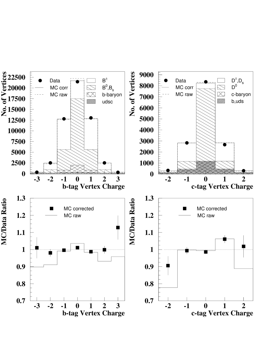
Figure 7: Top: vertex charge distributions for $y_{hem}>0.75$ $b$-tag (left) and $y_{hem}<0.4$ $c$-tag (right) hemispheres. The data (dots) are compared with MC predictions with or without tracking corrections. Bottom: the ratio of MC over data for before and after corrections

This tests directly the relevant secondary vertex tracks independent of the modeling of fragmentation track multiplicity. The $|Q|>1$ bins are particularly sensitive to tracking inefficiencies, while only weakly depend on heavy hadron decay multiplicity and production fractions.

5.3.2 IP tail

Another potential systematic source is the possible tails in the IP position determination which can cause large tagging asymmetries. The ${Z^{0}\rightarrow\mu^{+}\mu^{-}}$ events have no indication of systematic tail effects. A further study [24] is done by examining the distribution of the distance between the hemisphere axis drawn through the fitted event primary vertex in $r-\phi$ to the IP for 2-jet hadronic events with no secondary decay tracks.

There is no significant discrepancy between data and MC for 97-98 data, but there is a detectable tail in the 96 data with $\sim$100$\,\mu\rm m$ width for 0.5% of the events. The full effect of the tail is treated as a systematic uncertainty for the 96 data.

5.3.3 Geometric and temporal correlation effects

Besides the issue of the uncertainty in the overall tracking efficiency, MC modeling uncertainties on the efficiency nonuniformity due to local detector inefficiencies and time variations can lead to additional uncertainties on tagging correlations. The contribution of the $\theta$ and $\phi$ tagging efficiency dependence to the overall tagging efficiency correlation are estimated in section 5.1. We estimate the uncertainty of the MC modeling of $\theta$ and $\phi$ dependency, by comparing the hemisphere tagging fractions between data and MC for the $y_{hem}>0.75$ $b$-tag and representative $y_{hem}<0.4$ $c$-tag. There is a generally good agreement between the data and MC within the statistical errors. The only significant effect, the variation in $\phi$ for 96 data, due to electronics failures for some of the periods, is reasonably simulated by the MC. To estimate the correlation uncertainty, we simply take the ratio of the all input hemisphere tagging fractions between data and MC for each $\phi$ and $\theta$ bin, to reweight the MC true signal tagging efficiency for the corresponding bin, as an approximated deviation. The reweighted $\phi$ and $\theta$ dependent efficiencies are then used to recalculate the tagging efficiency correlation components as described in section 5.1. The change of the tagging correlation from the reweighting is taken as a systematic error. Note that correlation component calculations are insensitive to overall efficiency differences between data and MC which may enter in the reweighting, but only to shape variations. The resulting systematic errors on the geometrical correlations are summarized in Table 5. The correlation systematic error on $\Delta C_{b-tag}$ translates directly to the fractional error $\delta R_{b}/R_{b}$, and the error on the representative $c$-tag of $\Delta C_{c-tag}$ translates approximately to the fractional error $\delta R_{c}/R_{c}$. The use of data vs MC ratio unfortunately introduces statistical fluctuations on the estimated correlation change. A toy MC study indicates for example that the statistical fluctuation expected for the $\phi$ effect estimate is $\sim$0.00009 for 97-98 $b$-tag and as large as $\sim$0.0031 for the 96 $c$-tag. Some of the changes are consistent with statistical fluctuation, but we still conservatively take them as systematic uncertainties.

	$\Delta C_{b-tag}$		$\Delta C_{c-tag}$
	97-98	96	97-98	96
$\theta$ effect	0.00016	0.00181	0.00043	0.00337
$\phi$ effect	0.00027	0.00037	0.00030	0.00409
time dependence	-	0.00029	-	0.00055

Table 5: Correlation systematic uncertainties due to geometrical and time dependent effects.

For the time dependent effects on the tagging correlations there is a very good uniformity in the 97-98 data. The smaller 96 data sample does have significant time dependent effects, which contribute to the overall uncertainties. The resulting systematic errors on the temporal correlations for the 96 analysis are summarized in Table 5.

5.4 Event selection bias

The hadronic event selection flavor bias is evaluated from the MC for the basic hadronic event selection procedure and the last step of $N_{jet}<$4 cut separately. The event selection efficiencies and resulting bias on $R_{b}$ and $R_{c}$ are tabulated in Table 6.

Stage	Basic Had. Sel.	$N_{jet}<4$	Total
$uds$ efficiency	$58.330\pm 0.050\%$	$91.760\pm 0.037\%$	$53.524\pm 0.051\%$
$c$ efficiency	$58.592\pm 0.045\%$	$91.695\pm 0.033\%$	$53.725\pm 0.045\%$
$b$ efficiency	$58.694\pm 0.036\%$	$92.376\pm 0.025\%$	$54.220\pm 0.036\%$
$\Delta R_{b}$	$0.00089\pm 0.00016$	$0.00117\pm 0.00007$	$0.00207\pm 0.00017$
$\Delta R_{c}$	$0.00040\pm 0.00018$	$-0.00035\pm 0.00008$	$0.00005\pm 0.00020$

Table 6: Event selection efficiencies and flavor bias for the uncorrected MC.

The basic hadronic selection passes a slightly higher fraction of $b\mbox{${\overline{b}}$}$ events, which is expected from the known higher charged multiplicity and other observed kinematic differences of $b$-jets compared to $uds$. Given that the effect is only a few times the statistical error $\sigma$, we simply take the MC statistical error as an uncertainty for this stage. The $N_{jet}<4$ cut on the other hand has a more statistically significant effect. The rate of ${c\mbox{${\overline{c}}$}}$ events passing the $N_{jet}<4$ cut is consistent with that for $uds$ (most of the $\Delta R_{c}$ is actually the compensating effect of $R_{b}$ bias).

The effect of the $b$ quark mass on the $\geq 4$ jet rate has significant theoretical uncertainties. The JETSET 7.4 MC used for our analysis is in fact known to have excessive suppression of gluon radiation for heavy quarks [26], when comparing with data on 3 jet rates as used in the running $b$ quark mass measurements [25]. We use the DELPHI measurement [27] of the ratio $R_{4}^{bl}=f_{4}(\mbox{$b\mbox{${\overline{b}}$}$})/f_{4}(uds)$ to evaluate the event selection bias in our analysis for the $<4$ jet requirement, where $f_{4}$ denotes the fraction of events with $\geq 4$ jets. The DELPHI measurement using the Cambridge jet finder on all final state hadrons gives $R_{4}^{bl}=0.89\pm 0.02$ at $y_{\mbox{\tiny cut}}$=0.006, with only very small $y_{\mbox{\tiny cut}}$ dependence. The overall 4 jet rate at this $y_{\mbox{\tiny cut}}$ is very similar to the 4 jet rates using JADE Yclus jet finder on charged tracks with $y_{\mbox{\tiny cut}}$=0.02, as in our analysis. We use the PYTHIA 6.228 generator [28] as an intermediate reference to compute correction factors based on the ratios of ($1-R_{4}^{bl}$) with the same jet finding algorithms. We obtain a scaling factor of $S=0.50\pm 0.13$ to be applied to the raw 4-jet cut bias in the JETSET 7.4 MC. The uncertainty consists of equal contributions from the DELPHI measurement uncertainty and from the observed difference between using charged tracks and all final-state hadrons as input to the jet finder algorithms. Applying this scaling factor to the raw 4-jet bias of $\Delta R_{b}=0.00117$ in Table 6, we obtain a corrected 4-jet bias of $\Delta R_{b}=0.00059\pm 0.00015$. The event selection bias for ${c\mbox{${\overline{c}}$}}$ is consistent with zero and therefore no correction is applied for $R_{c}$.

As a crosscheck to verify the $R_{b}$ event selection bias estimate for the 4-jet cut, we also performed the analysis without the $N_{jet}<4$ cut for the larger 97-98 data sample. Taking into account the additional sensitivity to ${g\rightarrow{Q\overline{Q}}}$, we find the difference in measured $R_{b}$ due to the removal of $<4$-jet requirement is

$$R_{b}({\rm no\ <4\ jet\ cut})-R_{b}({\rm nominal\ analysis})=+0.00042\pm 0.00030\pm 0.00015$$

where the first error is the uncorrelated statistical uncertainty and the second error is the systematic error on the 4-jet cut bias as estimated above. The difference is consistent with zero within statistics.

5.5 Result stability checks

One possible source of systematic uncertainty is poor modeling of the $uds$ background that gives a secondary vertex due to badly reconstructed tracks. As a cross-check we tried to extract this effect from the data. We define a $uds$ tag by requiring no secondary vertex and no track with a normalized 3D impact parameter of more than 2$\sigma$. This tag identifies about 50% of the $uds$, 15% of the $c$ and 1.4% of the $b$ hemispheres. Adding this tag to the other ones, we fit for the same efficiencies as before plus the ratio of $uds$ giving a secondary vertex in data over Monte Carlo. We find a value of $1.1\pm 0.1$ for this ratio.

We also examine the variation of the $R_{b}$ result as a function of the minimum $y_{hem}$ cut for the $b$ tag, over a wide range of $y_{hem}$ cut, as shown in Fig. 8. The $R_{b}$ result is stable within the $1\sigma$ total uncertainty envelope.

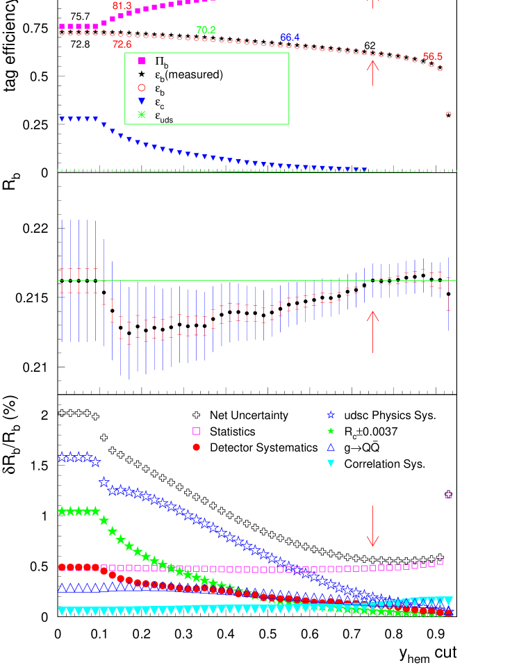
Figure 8: a) Tagging efficiencies and $b$ purity vs $y_{hem}$ cut. b) variation of the measured value of $R_{b}$, with the inner error bar being the uncorrelated statistical error w.r.t. the nominal cut and the outer bar total error. c) $R_{b}$ statistical and systematic error components as a function of the $b$-tag selection cut, for the 97-8 analysis. The net uncertainty does not include event selection uncertainties.

Since the $R_{c}$ measurement uses the full range of $y_{hem}$ values, there is no equivalent plot for this measurement. We do check the stability of the result by moving the boundary between the high purity charm tag (1) and the low purity charm tag (2) from 0.15 to 0.45 in increments of 0.05. We find that the $R_{c}$ result is stable within 0.0005. The low purity tags showed some difference in efficiency for charm events between data and Monte Carlo. Although we can reproduce the measured efficiency by varying some of the MC parameters in their allowed range we perform an additional cross-check by removing the low-purity tag 3 from the fit and re-measuring $R_{c}$. We find an insignificant shift of $+0.0009\pm 0.0014$ in 97-98 and $-0.0022\pm 0.0032$ in 96.

6 Conclusions

We have measured the hadronic branching ratio of the $Z^{0}$ to $b$ quark and $c$ quark with our 96-98 dataset of $\sim$400,000 hadronic $Z^{0}$ decays. The 96 and 97-98 results are combined, with all common systematic uncertainties, including detector uncertainties, treated as fully correlated. The combined results are:

$R_{b}$	=	0.21604	$\pm$0.00098(stat)	$\pm$0.00073(sys)	$\mp$0.00012($R_{c}$)
$R_{c}$	=	0.1744	$\pm$0.0031(stat)	$\pm$0.0020(sys)	$\mp$0.0006($R_{b}$)

For the $R_{b}$ measurement, combining this new measurement with our previously published result on the 93-95 data [3], we obtain:

$$R_{b}=0.21594\pm 0.00094{\mbox{(stat)}}\pm 0.00074{\mbox{(sys)}}\mp 0.00012(R_{c})$$

The relative weights in the combined average for the 93-95:96:97-98 (96:97-98) $R_{b}$ ($R_{c}$) measurements are 7:9:84 (11:89), dominated by the 97-98 result. These measurements are in good agreement with the Standard Model expectation of $R_{b}$=0.2156 (for $m_{t}$=178${\mathrm{\,Ge\kern-1.00006ptV\!/}c^{2}}$) and $R_{c}$=0.1723. They can be compared with the average of LEP measurements [29] from a total of $\sim$16 M hadronic $Z^{0}$ decays:

$R_{b}$	=	0.21643	$\pm$	0.00073
$R_{c}$	=	0.1691	$\pm$	0.0047

In conclusion, we have exploited the high resolution vertexing capability and the small and the stable SLC IP for a precision test of Standard Model through the measurements of heavy quark production fractions in $Z^{0}$ decays. Our new $R_{c}$ result is by itself more precise than the current world average [19]. These measurements confirm the Standard Model predictions at $\sim$0.6% precision for $R_{b}$ and 2.1% precision for $R_{c}$.

We thank the staff of the SLAC accelerator department for their outstanding efforts on our behalf. This work was supported by the U.S. Department of Energy and National Science Foundation, the UK Particle Physics and Astronomy Research Council, the Istituto Nazionale di Fisica Nucleare of Italy and the Japan-US Cooperative Research Project on High Energy Physics.

	$\delta R_{b}(10^{-5})$	$\delta R_{c}(10^{-5})$
MC statistics	13	91
${g\rightarrow{b\overline{b}}}$ 0.254$\pm$0.051%	-24	9
${g\rightarrow{c\overline{c}}}$ 2.96$\pm$0.38%	-23	-101
long lived light hadron production $\pm$10%	-1	-1
$D^{+}$ production $0.233\pm 0.028$	-10	-6
$D_{s}$ production $0.102\pm 0.037$	-11	-15
$c$-baryon production $0.065\pm 0.029$	-11	22
charm fragmentation	-18	18
$D^{0}$ lifetime $0.415\pm 0.004$ ps	-3	8
$D^{+}$ lifetime $1.057\pm 0.015$ ps	-2	5
$D_{s}$ lifetime $0.467\pm 0.017$ ps	-3	-3
$\Lambda_{c}$ lifetime $0.206\pm 0.012$ ps	-1	-91
$D$ decay multiplicity	-27	60
$D$ decay $K^{0}$	19	56
$D$ decay no-$\pi^{0}$	-9	12
$B$ lifetime $\pm 0.05$ ps	0	5
$B$ decay $\langle N_{ch}\rangle=5.73\pm 0.35$	-20	3
$b$ fragmentation	4	26
$\Lambda_{b}$ production fraction $0.074\pm 0.030$	5	-2
QCD hemisphere correlation	6	22
hard gluon radiation	-2	26
tag geometry dependency	9	17
tag time dependency	1	1
component correlation	14	45
tracking resolution	27	22
tracking efficiency	13	3
$\langle IP\rangle_{xy}$ tail	2	0
event selection bias	17	20
4 jet rate in $b$ events	15	0
$R_{c}=0.1723\pm 0.0037$	-12
$R_{b}=0.2157\pm 0.0010$		-62
Total (excl. $R_{b/c}$)	73	200

Table 7: Summary of systematic uncertainties for $R_{b}$ and $R_{c}$. A $-$ sign for an error means the value for $R_{q}$ goes down when this parameter is varied upward. The errors are assumed to be symmetric.

References

- [1]
-
[2]
ALEPH Collab, R. Barate et al.,
Phys. Lett. B 401 (1997) 150.
ALEPH Collab, R. Barate et al., Phys. Lett. B 401 (1997) 163.
DELPHI Collab, P. Abreu et al., Eur. Phys. J C10 (1999) 415.
L3 Collab, M. Acciari et al., Eur. Phys. J C13 (2000) 47.
OPAL Collab, G. Abbiendi et al., Eur. Phys. J C8 (1999) 217.
- [3] SLD Collab., K. Abe et al., Phys. Rev. Lett. 80 (1998) 660.
-
[4]
ALEPH Collab, R. Barate et al.,
Eur. Phys. J C4 (1998) 557.
DELPHI Collab, P. Abreu et al., Eur. Phys. J C12 (2000) 209.
DELPHI Collab, P. Abreu et al., Eur. Phys. J C12 (2000) 225.
OPAL Collab, K. Ackerstaff et al., Eur. Phys. J C1 (1998) 439.
ALEPH Collab, R. Barate et al., Eur. Phys. J C16 (2000) 597.
OPAL Collab, G. Alexander et al., Z. Phys. J C72 (1996) 1.
- [5] M. Breidenbach, IEEE Trans. Nucl. Sci. 33 (1986) 46.
- [6] SLD Collaboration, K. Abe et al., Phys. Rev. D53 (1996) 1023.
- [7] M.D. Hildreth et al., IEEE Trans. Nucl. Sci. 42 (1994) 451.
- [8] K. Abe et al., Nucl. Instr. Meth. A400 (1997) 287.
- [9] D. Axen et al., Nucl. Inst. Meth. A328 (1993) 472.
- [10] D. J. Jackson, D. Su and F.J. Wickens, Nucl. Inst. and Meth. A510, 233 (2003).
- [11] T. Sjöstrand, Comput. Phys. Commun. 82 (1994) 74.
-
[12]
P. N. Burrows, Z. Phys. C41 (1988) 375.
OPAL Collab., M.Z. Akrawy et al., Z. Phys. C47 (1990) 505. - [13] R. Brun et al., Report No. CERN-DD/EE/84-1 (1989).
- [14] A. S. Chou, Ph.D thesis, Stanford Univ., SLAC-R-578 (2001).
- [15] JADE Collab., W. Bartel et al., Z. Phys. C33 (1986) 23.
- [16] D. J. Jackson, Nucl. Inst. and Meth. A388, 247 (1997).
- [17] T. R. Wright, Ph.D thesis, U. of Wisconsin, SLAC-R-602 (2002).
- [18] The LEP Electroweak Working Group, D. Abbaneo et al., LEPHF/2001-01 (November 2001).
- [19] S. Eidelman et al., Phys. Lett. B 592, 1 (2004).
- [20] C. Peterson, D. Schlatter, I. Schmitt and P.M. Zerwas, Phys. Rev. D27 (1983) 105.
- [21] M.G. Bowler, Z. Phys. C11 (1981) 169.
- [22] D. Coffman et al., Phys. Lett.B263 (1991) 135.
- [23] G. Marchesini et al., Comp. Phys. Comm. 67 (1992) 465.
- [24] S.E Walston, Ph.D thesis, U. of Oregon, SLAC-R-728 (2004).
- [25] DELPHI Collab.: P. Abreu et al., Phys. Lett. B418 (1998), 430; A. Brandenburg, P. Burrows, D. Muller, N. Oishi and P. Uwer, Phys. Lett. B468 (1999), 168; ALEPH Collab.: R. Barate et al., Eur. Phys. J C18 (2000) 1; OPAL Collab.: G. Abbiendi et al., Eur. Phys. J C21 (2001) 411.
- [26] E. Norrbin and T. Sjöstrand, Nucl. Phys. B603 (2001), 297.
- [27] DELPHI Collab.: P. Bambade et al., Contributed paper 5-0139, ICHEP-04, Aug 2004, Beijing, China; DELPHI 2003-023 CONF 642 (2003). Publication in preparation.
- [28] T. Sjöstrand et al., Comp. Phys. Comm. 135 (2001) 238, hep-ph/0108264 (2001).
- [29] The LEP Collaborations, the LEP Electroweak Working Group and the SLD Electroweak and Heavy Flavor Working Groups, CERN-PH-EP/2004-069, hep-ex/0412015, Dec/2004.