Report of the Solar and Atmospheric Neutrino Experiments Working Group of the APS Multidivisional Neutrino Study

1 Executive Priority Summary

The highest priority of the Solar and Atmospheric Neutrino Experiment Working Group is the development of a real-time, precision experiment that measures the $pp$ solar neutrino flux. A measurement of the $pp$ solar neutrino flux, in comparison with the existing precision measurements of the high energy ⁸B neutrino flux, will demonstrate the transition between vacuum and matter-dominated oscillations, thereby quantitatively testing a fundamental prediction of the standard scenario of neutrino flavor transformation. The initial solar neutrino beam is pure $\nu_{e}$, which also permits sensitive tests for sterile neutrinos. The $pp$ experiment will also permit a significantly improved determination of $\theta_{12}$ and, together with other solar neutrino measurements, either a measurement of $\theta_{13}$ or a constraint a factor of two lower than existing bounds.

In combination with the essential pre-requisite experiments that will measure the ⁷Be solar neutrino flux with a precision of 5%, a measurement of the $pp$ solar neutrino flux will constitute a sensitive test for non-standard energy generation mechanisms within the Sun. The Standard Solar Model predicts that the $pp$ and ⁷Be neutrinos together constitute more than 98% of the solar neutrino flux. The comparison of the solar luminosity measured via neutrinos to that measured via photons will test for any unknown energy generation mechanisms within the nearest star. A precise measurement of the $pp$ neutrino flux (predicted to be 92% of the total flux) will also test stringently the theory of stellar evolution since the Standard Solar Model predicts the $pp$ flux with a theoretical uncertainty of 1%.

We also find that an atmospheric neutrino experiment capable of resolving the mass hierarchy is a high priority. Atmospheric neutrino experiments may be the only alternative to very long baseline accelerator experiments as a way of resolving this fundamental question. Such an experiment could be a very large scale water Cerenkov detector, or a magnetized detector with flavor and antiflavor sensitivity.

Additional priorities are nuclear physics measurements which will reduce the uncertainties in the predictions of the Standard Solar Model, and similar supporting measurements for atmospheric neutrinos (cosmic ray fluxes, magnetic fields, etc.). We note as well that the detectors for both solar and atmospheric neutrino measurements can serve as multipurpose detectors, with capabilities of discovering dark matter, relic supernova neutrinos, proton decay, or as targets for long baseline accelerator neutrino experiments.

Figure 1 shows a potential timeline for these experiments.

Figure 1: Timeline for future solar and atmospheric neutrino experiments.

2 Introduction

2.1 Discovery Potential

Both the first evidence and the first discoveries of neutrino flavor transformation have come from experiments which use neutrino beams provided by Nature. These discoveries were remarkable not only because they were unexpected—they were discoveries in the purest sense—but that they were made initially by experiments designed to do different physics. Ray Davis’s solar neutrino experiment [1] was created to study solar astrophysics, not the particle physics of neutrinos. The IMB [2, 3] and Kamiokande [4] experiments were hoping to observe proton decay, rather than study the (ostensibly relatively uninteresting) atmospheric neutrino flux. That these experiments and their successors [5, 6, 7, 8, 9, 10] have had such a great impact upon our view of neutrinos and the Standard Model underscores two of the most important motivations for continuing current and creating future solar and atmospheric neutrino experiments: they are naturally sensitive to a broad range of physics (beyond even neutrino physics), and they therefore have a great potential for the discovery of what is truly new and unexpected.

The fact that solar and atmospheric neutrino experiments use naturally created neutrino beams raises the third important motivation—the beams themselves are intrinsically interesting. Studying atmospheric neutrinos can tell us about the primary cosmic ray flux, and at high energies it may bring us information about astrophysical sources of neutrinos (see Report of Astrophysics Working Group) or perhaps even something about particle interactions in regimes still inaccessible to accelerators. For solar neutrinos, the interest of the beam is even greater: as the only particles which can travel undisturbed from the solar core to us, neutrinos tell us details about the inner workings of the Sun. The recent striking confirmation [9, 11, 12, 13] of the predictions of the Standard Solar Model [71] (SSM) are virtually the tip of the iceberg: we have not yet examined in an exclusive way more than 99% of the solar neutrino flux. The discovery and understanding of neutrino flavor transformation now allows us to return to the original solar neutrino project—using neutrinos to understand the Sun.

The fourth and perhaps strongest motivation for solar and atmospheric neutrino experiments is that they have a vital role yet to play in exploring the new physics of neutrinos. The beams used in these experiments give them unique sensitivity to some of the most interesting new phenomena. The solar beam is energetically broadband, free of flavor backgrounds, and passes through quantities of matter obviously unavaible to terrestrial experiments. The atmospheric beam is also broadband, but unlike the solar beam it has the additional advantage of a baseline which varies from tens of kilometers to many thousands.

2.2 Primary Physics Goals

In the work described here, we have chosen to focus on the following primary physics questions:

• Is our model of neutrino mixing and oscillation complete, or are there other mechanisms at work?

  To test the oscillation model, we must search for sub-dominant effects such as non-standard interactions, make precision comparisons to the measurements of other experiments in different regimes, and verify the predictions of both the matter effect and vacuum oscillation. The breadth of the energy spectrum, the extremely long baselines, and the matter densities traversed by solar and atmospheric neutrinos make them very different than terrestrial experiments, and hence measurements in all three mixing sectors—including limits on $\theta_{13}$—can be compared to terrestrial measurements and thus potentially uncover new physics.

• Is nuclear fusion the only source of the Sun’s energy, and is it a steady state system?

  Comparison of the total energy output of the Sun measured in neutrinos must agree with the total measured in photons, if nuclear fusion is the only energy generation mechanism at work. In addition, the comparison of neutrino to photon luminosities will tell us whether the Sun is in an approximately steady state by telling us whether the rate of energy generation in the core is equal to that radiated through the solar surface—the heat and light we see today at the solar surface was created in the interior $\sim$ 40,000 years ago, while the neutrinos are just over eight minutes old.

• What is the correct hierarchical ordering of the neutrino masses?

  Atmospheric neutrinos which pass through the Earth’s core and mantle will have their transformation altered due to the matter effect, dependent upon the sign of the $\Delta m^{2}_{13}$ mass difference. Future large scale water Cerenkov experiments may be able to observe this difference in the ratio of $\mu$-like to $e$-like neutrino interactions, while magnetized atmospheric neutrino experiments may be able to see the effect simply by comparing the number of detected $\nu_{\mu}$ to $\bar{\nu_{\mu}}$ events.

3 The Standard Solar Model and Solar Neutrino Experiments

The forty-year effort which began as a way to understand the Sun’s neutrino production ultimately taught us two remarkable things: that the Sun’s neutrinos are changing flavor between their creation in the solar interior and their detection on Earth, and that the Standard Solar Model’s predictions of the ⁸B flux of neutrinos was accurate to a degree well within its theoretical uncertainties.

Figure 2 summarizes the Standard Solar Model’s predictions for the neutrino fluxes and spectra. In Figure 2 the neutrinos labeled $pp$, $pep$, ⁷Be, ⁸B, and hep belong to the ‘$pp$-chain’ which for a star like the Sun dominates over those from the CNO cycle. Of the neutrinos in the $pp$ chain, those from the initial reaction $p+p\rightarrow d+e^{+}+\nu_{e}$ make up over 92% of the entire solar flux.

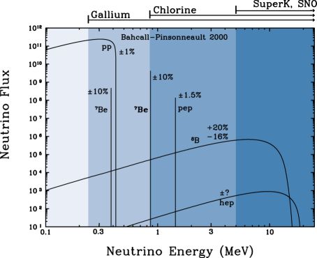
Figure 2: Differential Standard Solar Model neutrino fluxes [14].

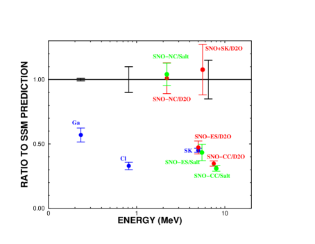
Figure 3: Comparison of measurements to Standard Solar Model predictions.

Figure 3 shows the past forty years of measurements of the solar neutrino fluxes. In the figure, the measurements are plotted in terms of their respective neutrino energy thresholds. The experiments divide into two classes: radiochemical experiments like the original Davis Chlorine detector, and real-time experiments like Super-Kamiokande and SNO.

The radiochemical experiments do not provide any direct spectral information about the solar fluxes, but rather make inclusive measurements of all neutrino sources above their particular reaction threshold. For the Gallium based experiments such as SAGE [6] and Gallex [7], this sensitivity extends all the way down to the $pp$ neutrinos but includes all neutrinos above the threshold of 0.233 MeV (even neutrinos of the CNO cycle should they exist). The Chlorine threshold is above that of the $pp$ neutrinos, but is sensitive to the neutrinos from ⁷Be and ⁸B, as well as potential CNO neutrinos. For all radiochemical experiments, the interpretation of the observed rates as measurements of neutrino mixing assume that the Standard Solar Model calculated fluxes are correct within their theoretical uncertainties. In addition, the best values of the mixing parameters are obtained when the ‘luminosity constraint’ is imposed, requiring the sum of all the energy radiated by the Sun through neutrinos to agree with that radiated through photons.

To date, the real-time experiments have all been water Cerenkov experiments. As such, their neutrino energy thresholds are relatively high, and they are sensitive exclusively to the neutrinos from the solar ⁸B reaction (if the flux of neutrinos from the hep reaction were high enough they would also be included in the measurements). This exclusivity has had a great advantage: comparison of the number of neutrinos measured through the charged current (CC) reaction in SNO’s heavy water ($\nu_{e}+d\rightarrow e^{-}+p+p$) to that measured via the elastic scattering (ES) of electrons in Super-Kamiokande’s light water ($\nu+e^{-}\rightarrow\nu+e^{-}$) allowed the first model-independent demonstration of the transformation of solar neutrinos [8, 9]. SNO’s subsequent measurement of the rate of neutral current (NC) events in D₂O ($\nu+d\rightarrow\nu+n+p$) provided the first direct measurement of the total active ⁸B flux [11]. In both cases—the combination of the SNO and Super-Kamiokande measurements as well as the SNO NC measurement, the measurements of the ⁸B flux were in excellent agreement with the predictions of the Standard Solar Model for that flux. The SNO measurements therefore allow measurements of neutrino mixing parameters without any reliance upon the predicted Standard Solar Model ⁸B neutrino flux.

The real-time experiments also allow searches for time-dependent variations (such as a Day/Night asymmetry) and comparisons of the observed recoil electron spectrum to expectations for the ⁸B neutrinos. As of yet, no significant asymmetry or distortion of the spectrum has been observed.

With the integral measurements of the radiochemical experiments, the differential real-time exclusive measurements of the water Cerenkov experiments, and the fluxes from the Standard Solar Model for all but the ⁸B neutrinos, the allowed region of mixing parameters is restricted to the large mixing angle region (LMA). Figure 4 shows this allowed region, for all solar neutrino data.

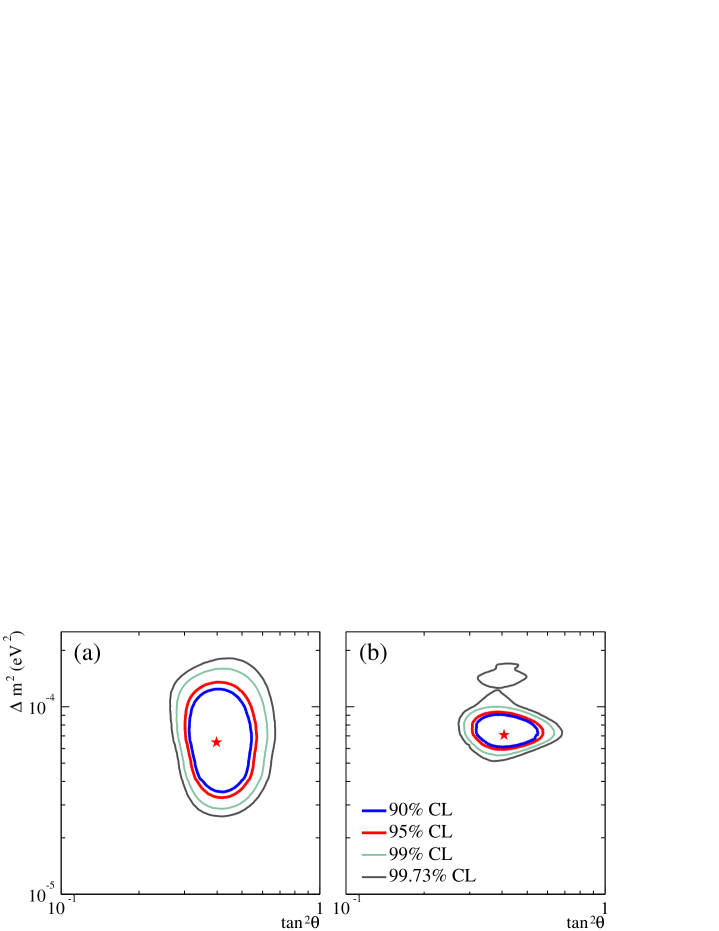
Figure 4: Measurements of the mixing parameters for (a) all solar data and (b) solar+KamLAND data [13], before the new results from the Neutrino 2004 conference.

3.1 Testing the Model of the Sun

The idea that the Sun generates power through nuclear fusion in its core was first suggested in 1919 by Sir Arthur Eddington, who pointed out that the nuclear energy stored in the Sun is “well-nigh inexhaustible”, and therefore could explain the apparent age of the Solar System. Hans Bethe developed the first detailed model of stellar fusion, in which the CNO cycle was thought to be the dominant process.

Despite the obvious appeal of the theory, simple observations of the solar luminosity are not enough to demonstrate that nuclear fusion is, in fact, the solar energy source. As John Bahcall wrote in 1964:“No direct evidence for the existence of nuclear reactions in the interiors of stars has yet been obtained…Only neutrinos, with their extremely small interaction cross sections, can enable us to see into the interior of a star and thus verify directly the hypothesis of nuclear energy generation in stars.” [16]. The idea only became feasible when Bahcall and Davis showed that a reasonably-sized Chlorine detector could observe the neutrinos at ⁷Be energies and higher.

No one anticipated that it would take nearly four decades and eight different experiments before Bahcall and Davis’s original idea of testing the model of the Sun in detail could become a reality. With the measurements of SNO and the KamLAND reactor experiment, the problem of neutrino mixing can now be decoupled from the study of neutrinos as the signature of solar energy generation.

What we know: the Standard Solar Model correctly predicts the flux of ⁸B neutrinos measured by SNO, and that globally fitting all the solar neutrino data (and the data from the KamLAND reactor experiment) for the neutrino fluxes and mixing parameters, provides good agreement with the Standard Solar Model. Table 1, reproduced here from Ref. [17], shows the resultant mixing angle and the ratio of the fitted fluxes to the predictions of the SSM, that is

$$f=\frac{\phi_{\rm fit}}{\phi_{\rm SSM}}.$$

Analysis	$\tan^{2}\theta_{12}$	$f_{B}$	$f_{Be}$	$f_{pp}$
A	$0.45^{+0.04}_{-0.06}$ (${}^{+0.24}_{-0.16}$)	$0.99^{+0.05}_{-0.03}$ (${}^{+0.14}_{-0.13}$)	$0.13^{+0.41}_{-0.13}$ (${}^{+1.27}_{-0.13}$)	$1.38^{+0.18}_{-0.25}$ (${}^{+0.47}_{-0.75}$)
A + lum	$0.40^{+0.06}_{-0.04}$ (${}^{+0.23}_{-0.12}$)	$1.02^{+0.03}_{-0.05}$ (${}^{+0.12}_{-0.14}$)	$0.58^{+0.26}_{-0.25}$ (${}^{+0.81}_{-0.58}$)	$1.03^{+0.02}_{-0.02}$ (${}^{+0.05}_{-0.06}$)
B + lum	$0.41^{+0.05}_{-0.05}$ (${}^{+0.22}_{-0.13}$)	$1.01^{+0.04}_{-0.04}$ (${}^{+0.13}_{-0.13}$)	$0.93^{+0.25}_{-0.63}$ (${}^{+0.80}_{-0.93}$)	$1.02^{+0.02}_{-0.02}$ (${}^{+0.06}_{-0.06}$)

Table 1: Allowed neutrino parameters with free $p-p$, ⁷Be, and ⁸B solar neutrino fluxes: with and without luminosity constraint, from Ref. [17]. For all cases presented in this table, $\Delta m^{2}=7.3^{+0.4}_{-0.6}\times 10^{-5}{\rm eV^{2}}$ The results given here were obtained using all the currently available data from the solar  [7, 8, 11, 12, 10, 13, 18, 19] and KamLAND [20] neutrino experiments. All other (much less important) solar neutrino fluxes are assumed to have the standard solar model (BP00) predicted values and uncertainties.

The top row of Table 1 shows the fluxes without the luminosity constraint imposed, and we can see that the best fit $pp$ and ⁷Be neutrino fluxes have very large uncertainties and in fact do not agree with their SSM values (nor do they even obey the luminosity constraint itself). The ⁸B flux, which is constrained by the SNO neutral current measurements, stays close to its SSM value even if the luminosity constraint it not imposed. The second row of Table 1 is the same fit as in the first row, but now with the luminosity constraint imposed, and the third row is the same as the second, but with the CNO neutrino fluxes treated as free parameters. The important points to take from Table 1 are:

• Without the luminosity constraint, the $pp$ and ⁷Be fluxes are very poorly known, and the luminosity constraint is violated

• Even with the luminosity constraint, the ⁷Be flux is still very poorly determined, with uncertainties as large as 40%

• With the luminosity constraint, the $pp$ flux is known with a precision, $\pm 2$%, comparable to but still larger than the theoretical uncertainty, $\pm 1$% in the SSM prediction.

If we are to test the Standard Solar Model further, we therefore first need to measure the ⁷Be neutrinos. The planned measurements (see Section 3.4.1) are likely to improve knowledge of this flux significantly over what is now known. The measurements of the ⁷Be flux can also give us direct information about some of the critical parts of the Standard Solar Model, such as the ratio of rates of ³He+⁴He to ³He+³He [21]. In addition, a measurement of ⁷Be will improve the determination of the $pp$ neutrino flux from the Gallium experiments [19, 7] to which both $pp$ and ⁷Be neutrinos contribute to the rate. With the luminosity constraint, the $pp$ flux will be determined with a precision 2 to 4 times better than presently known (2$\%$), and test the precise prediction of the $pp$ SSM (1$\%$) [17].

An exclusive, real-time measurement of the $pp$ flux can provide us with an even more general test of the Standard Solar Model. In combination with the planned (and necessary) ⁷Be measurements and the existing ⁸B measurements, a $pp$ measurement will allow a precise test of the luminosity constraint itself, by comparing the inferred luminosity based on the neutrino fluxes with the observed photon luminosity. Such a test will tell us whether there are any energy generation mechanisms beyond nuclear fusion. In addition, we will learn whether the Sun is in a steady state, because the neutrino luminosity tells us how it burns today, while the photons tell us how it burned over 40,000 years ago. The current comparison of these luminosities is not very precise [17]:

$$\frac{L_{\odot}{\rm(neutrino-inferred)}}{L_{\odot}}~{}=~{}1.4^{+0.2}_{-0.3}\left({}^{+0.7}_{-0.6}\right).$$ (1)

We see that, at 3$\sigma$, the inferred luminosity can be 2.1 times larger than the measured photon luminosity, or 0.8 times smaller. The fact that the solar neutrino flux is overwhelmingly $pp$ neutrinos means that the precision of this comparison approximately scales with the precision of a measurement of the $pp$ flux—a measurement with a precision of 5% will reduce the uncertainties on this comparison to $\sim$4%.

We also note that, although not explicitly listed in Table 1, a measurement of the flux of neutrinos from the $pep$ reaction can provide much of the same information as the $pp$ measurements, if we are willing to make the Standard Solar Model assumption that the rates of the two reactions are strongly coupled.

3.2 Testing the Neutrino Oscillation Model

The idea that the Standard Model ‘accommodates’ the new found neutrino properties must recognize that the oscillation model of neutrino flavor transformation is just that—a model—and until we test that model with the kind of precision with which we have explored the rest of particle physics, we do not know whether it is in fact a satisfactory description of neutrinos. Even if we accept that the combination of the atmospheric and the solar results taken together are compelling evidence that flavor transformation in the neutrino sector is explained by the additional seven new Standard Model parameters, we as yet have no experimental evidence that the mixing involves three flavors in the way it does in the quark sector. We even have evidence to the contrary—the results of the LSND experiment, in combination with the results in the solar and atmospheric sector, point to either the existence of a fourth family or perhaps even stranger physics, such as a violation of CPT symmetry.

To test the model, therefore, we need to look directly for evidence of sub-dominant effects (Section 3.2.1), verify some of the basic predictions of the model like the matter effect (Section 3.2.2), and compare the predictions of the model across different physical regimes (Sections 3.2.3 and 3.2.4). The luminosity test described in the previous section (Section 3.1) is its own global test of neutrino properties. For example, were the neutrino luminosity to fall substantially short of the total luminosity, it could be evidence of energy loss to sterile neutrino species.

3.2.1 Other Transformation Hypotheses

Neutrino masses and mixing are not the only mechanism for neutrino flavor oscillations. They can also be generated by a variety of forms of nonstandard neutrino interactions or properties. In general these alternative mechanisms share a common feature: they require the existence of an interaction (other than the neutrino mass terms) that can mix neutrino flavours. Among others this effect can arise due to:

Violation of Equivalence Principle (VEP) [22]:
(non universal coupling of neutrinos $\gamma_{1}\neq\gamma_{2}$
to gravitational potential $\phi$)	${\lambda}=\frac{\pi}{E|\phi|\delta\gamma}$
Violation of Lorentz Invariance (VLI) [24]:
(non universal asymptotic velocity of neutrinos $v_{1}\neq v_{2}$)	$\lambda=\frac{2\pi}{E\delta v}$
Non universal couplings of neutrinos q $k_{1}\neq k_{2}$
to gravitational torsion strength $Q$ [23]	$\lambda=\frac{2\pi}{Q\delta k}$
Violation of Lorentz Invariance (VLI)
due to CPT violating terms [26] $\bar{\nu}_{L}^{\alpha}{b_{\mu}^{\alpha\beta}}\gamma_{\mu}\nu_{L}^{\beta}$	${\lambda}=\pm\frac{2\pi}{{\delta b}}$
Non-standard $\nu$ interactions in matter [25]:
$G_{F}{\varepsilon_{\alpha\beta}}(\overline{\nu_{\alpha}}\gamma^{\mu}\nu_{\beta})(\overline{f}\gamma_{\mu}f)$	${\lambda}=\frac{2\pi}{2\sqrt{2}G_{f}\;N_{f}\;\sqrt{\varepsilon_{\alpha\beta}^{2}+(\varepsilon_{\alpha\alpha}-\varepsilon_{\beta\beta})^{2}/4}}$

where $\lambda$ is the oscillation length.

From the point of view of neutrino oscillation phenomenology, the most relevant feature of these scenarios is that, in general, they imply a departure from the $E^{1}$ ($\lambda=\frac{4\pi E}{\Delta m^{2}}$) energy dependence of the oscillation wavelength.

Some of these scenarios have been invoked in the literature as explanations for the solar neutrino data alternative to mass oscillations. Prior to the arrival of KamLAND, some of them could still provide a good fit [27] to the data.

The observation of oscillations in KamLAND with parameters which are consistent with solar LMA oscillations clearly rules out these mechanisms as dominant source of the solar neutrino flavor transitions. However they may still exist at the sub-dominant level. This raises the question of to what point the possible presence of these forms of new physics (NP), even if sub-dominant, can be constrained by the analysis of solar and atmospheric data. Or, conversely, to what level our present determination of the neutrino masses and mixing is robust under the presence of phenomenologically allowed NP effects.

At present, there is no general analysis in the literature which answers these questions quantitatively. However one may argue that (unlike for atmospheric neutrinos), existing data on solar neutrinos by itself is unlikely to provide strong constraints on these forms of NP. Therefore, as long as the KamLAND data is not affected by these NP effects, there should be still more room for these effects in the analysis of the solar+KamLAND than there is in the corresponding analysis of atmospheric data. The reason for this is the scarce information from solar neutrino data on the energy dependence of the $\nu_{e}$ survival probability $P_{ee}$, as illustrated in Fig.5 where we show the results of a fit to the observed solar rates in terms of the averaged $P_{ee}$ for three energy regions of the solar neutrino spectrum (from Ref.[28]).

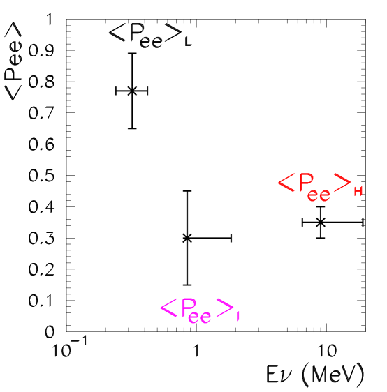
Figure 5: Reconstructed values of the survival probability of solar neutrinos in different energy ranges from a fit to the observed rates.

One illustrative example of this conclusion can be found in Ref. [30, 31]. The authors of these works find that the inclusion of somewhat large but still allowed non-standard neutrino interactions affecting the propagation of neutrinos in the Sun and Earth matter can shift the allowed region of oscillation parameters in the solar+KamLAND analysis to lower $\Delta m^{2}$ values without spoiling the quality of the fit.

Recently, there has been a suggestion that the mass varying neutrino (MaVaNs) hypothesis, put forward as an explanation of the of the origin of the Dark Energy and the coincidence of its magnitude with the neutrino mass splittings, may produce matter effects which will alter the solar and atmospheric neutrino oscillations [29]. This hypothesis can be made to fit simultaneously the solar, atmospheric, and LSND results.

3.2.2 MSW Effect

One of the predictions of the neutrino oscillation model is that matter can strongly affect the neutrino survival probability (the ‘MSW effect’ [45]). The effect arises because matter is made out of first generation material—the $\nu_{e}$’s interact with electrons via both charged current and neutral current channels, while at solar neutrino energies the other active flavor eigenstates have only neutral current interactions. The resultant difference in the forward scattering amplitudes makes the matter of the Sun birefringent to neutrinos, and the oscillation already caused by the neutrino mass differences can be enhanced by this additional dispersion. Beyond being a confirmation of our new model of neutrinos, the MSW effect is a beautiful phenomenon in its own right: as the neutrinos propagate from solar center to surface, the Sun’s changing density alters the effective mixing angles in an energy-dependent way, leaving its quantum mechanical imprint for us to observe on Earth.

The effective Hamiltonian for two-neutrino propagation in matter can be written conveniently in the familiar form [45, 46, 47, 49, 50, 51]

$$H~{}=~{}\left(\begin{array}[]{cc}\frac{\Delta m^{2}cos2\theta_{12}}{4E}-\frac{\sqrt{2}G_{\rm F}n_{\rm e}}{2}&\frac{\Delta m^{2}sin2\theta_{12}}{2E}\\ \frac{\Delta m^{2}sin2\theta_{12}}{2E}&-\frac{\Delta m^{2}cos2\theta_{12}}{4E}+\frac{\sqrt{2}G_{\rm F}n_{\rm e}}{2}\end{array}\right)\,.$$ (2)

Here $\Delta m^{2}$ and $\theta_{12}$ are, respectively, the difference in the squares of the masses of the two neutrinos and the vacuum mixing angle, $E$ is the energy of the neutrino, $G_{\rm F}$ is the Fermi coupling constant, and $n_{\rm e}$ is the electron number density at the position at which the propagating neutrino was produced.

The relative importance of the MSW matter term and the kinematic vacuum oscillation term in the Hamiltonian be parameterized by the quantity, $\beta$, which represents the ratio of matter to vacuum effects [17]. From equation 2 we see that the appropriate ratio is

$$\beta=\frac{2\sqrt{2}G_{F}n_{e}E_{\nu}}{\Delta m^{2}}\,.$$ (3)

The quantity $\beta$ is the ratio between the oscillation length in matter and the oscillation length in vacuum. In convenient units, $\beta$ can be written as

$$\beta=0.22\,\left[\frac{E_{\nu}}{1~{}{\rm MeV}}\right]\,\left[\frac{\mu_{e}\rho}{100~{}{\rm g~{}cm}^{-3}}\right]\,\left[\frac{7\times 10^{-5}eV^{2}}{\Delta m^{2}}\right]\,,$$ (4)

where $\mu_{e}$ is the electron mean molecular weight ($\mu_{e}\approx 0.5(1+X)$, where X is the mass fraction of hydrogen) and $\rho$ is the total density, both evaluated at the location where the neutrino is produced. For the electron density at the center of the standard solar model, $\beta=0.22$ for $E=1$MeV and $\Delta m^{2}=7\times 10^{-5}{\rm eV^{2}}$.

There are three explicit signatures of the MSW effect which can be observed with solar neutrinos. The first is the ‘Day/Night’ effect in which $\nu_{e}$’s which have been transformed by the matter of the Sun into $\nu_{\mu}$’s and $\nu_{\tau}$’s are changed back to $\nu_{e}$’s as they pass through the Earth—the coherent regeneration of $K^{0}_{S}$’s is a fair analogy. As the regeneration is only appreciable for large path lengths, the number of $\nu_{e}$’s observed by a detector at night will be larger than during the day.

The second signature of the MSW effect is a distortion of the energy spectrum, in the region of the transition from matter-dominated to vacuum-dominated oscillations. The energy dependence of the matter mixing angles and eigenstates leads to energy-dependent survival probabilities which are different from those for simple vacuum mixing. Figure 6 shows the turnup in the survival probabilities for some of the mixing parameters in the LMA region.

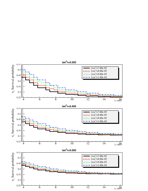
Figure 6: ⁸B solar neutrino survival probabilities in the LMA region.

The third signature is the observation of vacuum-dominated mixing at low energies [17]. When the parameter $\beta$ given in Eqn. 4 is greater than 1, the neutrino flavor transformation is dominated by matter effects, which occurs for the highest energy ⁸B neutrinos. Figure 7 shows the change in survival probability as the neutrino energies are lowered from the ⁸B energies down to $pp$ energies. The clear transition from matter-dominated to vacuum-dominated oscillations can be seen, and this transition region is the same as that shown in Figure 6. What Figure 7 shows is that a demonstration of the matter effect can be made by comparing the measured survival probability at high energies to that at low energies.

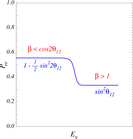
Figure 7: Transition between vacuum and matter-dominated flavor transformation, as a function of energy, from Ref. [17].

Based upon the results of the solar neutrino experiments and the KamLAND experiment, we know that the mixing parameters are in a region where the MSW effect plays an important role. As of yet, we have not directly seen any of its specific signatures. We conclude that Nature has been unkind—that the parameters are ‘unlucky’. Or perhaps we have not looked hard enough.

Below we discuss the prospects for identifying each of these signatures.

• Day/Night Asymmetry

  Both the Super-Kamiokande [15] and SNO [12] experiments have looked for a Day/Night asymmetry in the flux of ⁸B solar neutrinos. A measurement of a Day/Night asymmetry is perhaps the cleanest of the signatures of the matter effect, because the vast majority of experimental uncertainties cancel in the asymmetry ratio. The asymmetry is a function both of the energy and the zenith angle of the incident neutrinos, and so often the measurements are published as ‘Day/Night spectra’, occasionally binned or fit in distributions of zenith angle.

  Currently, only SNO and Super-Kamiokande are operating in a regime where a Day/Night asymmetry might be observable. In both cases, however, the measurements are statistically limited. Figure 8, from Ref. [32] shows contours of Day/Night asymmetry expected for SNO, overlaid with the LMA region of mixing parameters, and we can see that the asymmetry is small, even for the lowest allowed $\Delta m^{2}$ values.

  

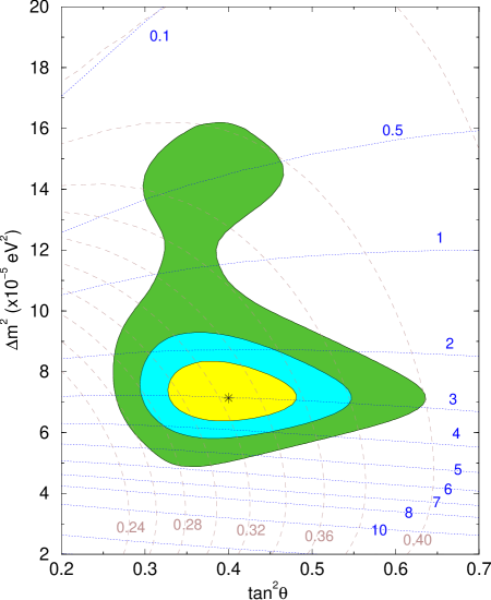
  Figure 8: Contours of expected Day/Night asymmetry, shown as the horizontal dotted lines labeled in %, overlain on the LMA region [32].

  To observe a Day/Night asymmetry with high significance will require a much larger real-time ⁸B experiment. Some of the proposals for new megaton-scale water Cerenkov detectors [33, 34] have included a low background region in the detector whose goal will be to observe the ⁸B neutrinos. With a fiducial volume at least seven times that of Super-Kamiokande, a photocathode coverage of at least 40%, and an energy threshold of 6 MeV, a large water Cerenkov detector could see the expected LMA Day/Night asymmetry of 2% with a significance of $\sim 4\sigma$ in roughly 10 years of running [35].

• Spectral Distortion

  To observe the rise in survival probability shown in Figure 6, real-time solar neutrino experiments capable of observing the ⁸B flux are needed. Both SNO and Super-Kamiokande have looked for signs of a distortion in the spectrum of observed recoil electrons, and they do not see any significant effect.

  To see the spectral distortion, SNO or Super-K will need to lower their energy thresholds—when convolved with the differential cross sections and the detector energy resolutions, the change in survival probability does not become noticeable until an electron recoil energy below 5 MeV or so. Investigations into the feasibility of background reduction in these experiments to see the distortion are underway.

  We note that there are currently no other experiments planned whose primary goal is to directly probe this region.

• Low E/High E Survival Probability Comparisons

  The Super-Kamiokande and SNO measurements have given us the survival probabilities for the high energy end of the solar neutrino spectrum, and so they have mapped out the matter-dominated survival region shown in the upper end Figure 7. The Chlorine and Gallium experiments, in combination with the predictions of the Standard Solar Model, have told us that the survival probability at low energies looks like the expectation from vacuum-dominated oscillations. Unfortunately, the integral nature of the low energy experiments means that they must rely on the assumption that the Standard Solar Model predictions for the various neutrino sources is correct. In particular, the inferences drawn from the radiochemical measurements assume the neutrino cross sections can be multiplied by a constant survival probability independent of energy, and neglect correlations among the systematic uncertainties. In addition, the CNO neutrinos are typically neglected when calculating the survival probabilities from these experiments. As Table 1 shows, the for a fit which includes all uncertainties, the resulting overall uncertainties are currently too large for a quantitative test of the MSW scenario. We therefore need exclusive measurements of the ⁷Be and $pp$ neutrino fluxes to unambiguously demonstrate the vacuum/matter transition with solar neutrinos.

3.2.3 Precision Comparisons in the (1,2) Sector

The strongest test of our model of neutrino flavor transformation is to compare the predictions over as wide a physical range as possible. The model predicts that seven fundamental parameters are all that is needed to explain every possible observation of neutrino flavor transformation regardless of lepton number, flavor, energy, baseline, or intervening matter. As it happens, even fewer parameters are needed to explain the observations which have been made so far, because the difference in the neutrino masses and the sizes of the mixing angles are such that most experiments can be treated as involving just two flavors.

The first precision test across experimental regimes is the comparison of the measurements of the KamLAND experiment to the solar neutrino experiments [20]. KamLAND sees a transformation signal with a range of parameters which include the solar LMA region, yet it differs in nearly every relevant way from the solar experiments: it looks at reactor antineutrinos rather than neutrinos; it has a medium baseline (150 km) rather than the $150\times 10^{6}$ km solar baseline; it looks for disappearance rather than SNO’s inclusive appearance; it is sensitive only to vacuum oscillations rather than matter-enhanced oscillations. Figure 9, from Ref. [36], shows the allowed regions of the mixing parameters determined by KamLAND overlain on the LMA region determined by the solar experiments. The fact that there is overlap between the two regions, and that the best fit point agrees within the measurement uncertainties, is remarkable confirmation of the oscillation model.

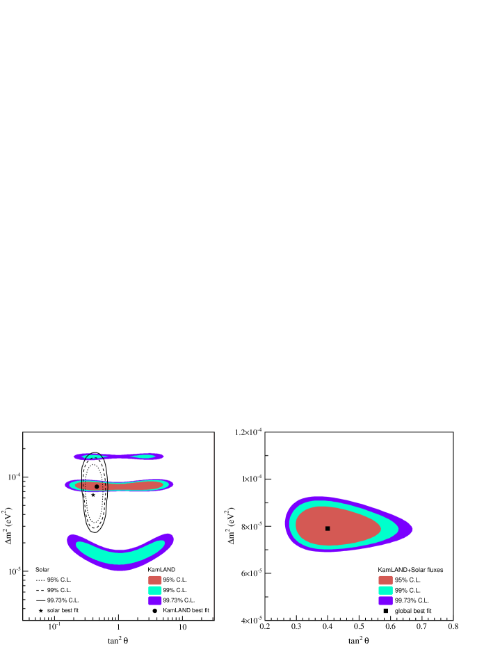
Figure 9: Allowed regions of mixing parameters determined by KamLAND, compared to solar measurements, for the most recent [36] results.

To go further, and explore some of the possibilities for new physics described in Section 3.2.1, we need to improve the precision on the measurements of the mixing parameters in the two regimes. The most recent KamLAND results [36] have improved the statistical precision of the initial measurements by roughly a factor of four, eliminating some of the regions in $\Delta m^{2}_{12}$ which were outside the region measured by the solar experiments. The possibility of a more precise reactor-based (1,2) sector experiment is also being discussed, perhaps in conjunction with a reactor experiment to measure the value of $\sin^{2}2\theta_{13}$ (see Report of Reactor Working Group).

SNO will soon publish updated results from the Phase II (salt) data, which will bring some improvements on the precision from the solar side. The next phase of SNO will reduce the uncertainties on the mixing angle further. While a ⁷Be measurement is not expected to improve the measurements of the mixing parameters, an exclusive measurement of the $pp$ flux (or a measure of the $pep$ flux) can have a substantial effect on the mixing parameters, depending on the precision of the measurement. Figure 10 shows the improvements on $\tan^{2}\theta_{12}$ that could come from a $pp$ measurement, allowing the $pp$, ⁷Be, ⁸B, and CNO neutrinos as free parameters, subject only to the luminosity constraint.

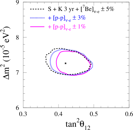
Figure 10: Improvements in mixing angle determination for hypothetical $pp$ experiments, including future KamLAND and ⁷Be measurements. From Ref [17].

3.2.4 Precision Comparisons of $\theta_{13}$

Like the (1,2) sector, measurements of the (1,3) parameters with solar neutrino experiments provide tests of the oscillation model in a very different regime than either reactor or accelerator experiments. In particular, measurements of $\theta_{13}$ with solar experiments are essentially independent of the value of $\Delta m^{2}_{23}$, unlike either the accelerator or reactor experiments. At solar neutrino energies, and the range of allowed values of $\Delta m^{2}_{13}$, the matter effect (unfortunately) does not play a significant role in the (1,3) transformation. However, we still expect to see (1,3) effects due to vacuum mixing.

A global analysis of all available data by Maltoni et al. [52] (but without the most recent value for $\Delta m_{23}^{2}$ or most recent KamLAND measurements [36]) gives $\theta_{13}=4.4_{-4.4}^{+6.3}$ degrees (2 $\sigma$). The current situation is well summarized in Figure 8 of [52], which we reproduce here (Fig. 11) superimposed with the most recent range for $\Delta m_{23}^{2}$. One can see that near the low end of the mass range the tightest limits on $\theta_{13}$ are already coming from solar neutrinos and KamLAND. The relationship between these experiments and $\theta_{13}$ began to be explored even before results were available from KamLAND [54].

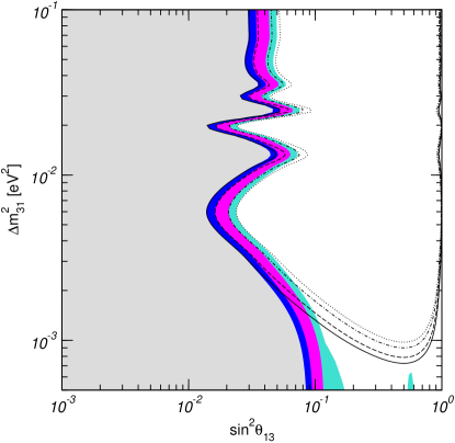
Figure 11: Limits on $\theta_{13}$ from Chooz (lines, 90%, 95%, 99%, and 3$\sigma$), and from Chooz+solar+KamLAND (colored regions) [52].

Ref. [59] has performed a fit to existing solar neutrino and KamLAND data, to investigate the effects of new solar measurements on the limits for $\theta_{13}$, and what follows is described in more detail there. The fit includes 5 unknowns, the 3 (total active) solar fluxes $\phi_{1}$, $\phi_{7}$, and $\phi_{8}$, and two mixing angles, $\theta_{12}$ and $\theta_{13}$. The mass-squared difference $\Delta m_{12}^{2}$ is fixed by the “notch” in the KamLAND reactor oscillation experiment, and $\Delta m_{23}^{2}$ by the atmospheric neutrino data. The fit parameters that are approximately normally distributed are $\phi_{1}$, $\phi_{7}$, $\phi_{8}$, $\sin^{2}\theta_{12}$, and $\cos^{4}\theta_{13}$.

Solar plus KamLAND data already provide some constraint on $\cos^{4}\theta_{13}$, with the corresponding angle $\theta_{13}=7.5_{-7.5}^{+4.8}$ degrees. The expected statistical improvements from the KamLAND experiment reduce the overall uncertainties somewhat—in particular $\theta_{13}$ is non-zero at 1 $\sigma$. The reason the improvement is not better is the growth of the correlation coefficient between the mixing parameters, which is as large as -0.906. Further improvements cannot be made without breaking that correlation.

The way to break the correlation is find a way of measuring the (1,2) parameters independently from the (1,3) parameters. Luckily, the MSW effect, which acts only in the (1,2) sector for solar neutrinos, can provide this independent measure. The transition between the vacuum- and matter-dominated regimes shown in Figure 7 shows that better measurements in the low energy regime can provide a lever arm to distinguish the (1,2) from the (1,3) effects. Unfortunately, reducing the uncertainties on the Gallium experiments (by, for example, understanding the cross sections better) does not help very much. The difficulty is that the ⁷Be flux is not well determined and thus floats against the survival probability $P_{ee}$. The strong correlation between the low-energy fluxes $\phi_{1}$ and $\phi_{7}$ could in the future be broken by a ⁷Be experiment, either CC or ES, or by a robust prediction of ⁷Be within the demonstrably reliable Standard Solar Model [71]. For the latter, a new high-precision determination of the ³He($\alpha,\gamma$)⁷Be cross section is needed. For concreteness at this point, we take a CC experiment with a precision of 5%. Table 2 shows that the low-energy fluxes are individually determined twice as precisely and there is some improvement in the separation of the mixing angles. Both an improved Ga rate and a ⁷Be determination are needed to obtain this improvement; either by itself is ineffective.

Table 2: Fitted fluxes and mixing parameters under the assumption of a putative CC ⁷Be experiment that measures $\phi_{7}$ to be 0.511 to an accuracy of 5%, as well as the KamLAND statistical improvements and the improved SNO CC/NC ratio.

Parameter	$\phi_{1}$	$\phi_{7}$	$\phi_{8}$	$\sin^{2}\theta_{12}$	$\cos^{4}\theta_{13}$
Value	6.00	0.525	$5.33\times 10^{-4}$	0.330	0.955
1-$\sigma$ error	0.06	0.06	$0.21\times 10^{-4}$	0.025	0.025
$\chi^{2}$	3.67
Correlation Matrix
$\phi_{1}$	1	-0.909	0.502	-0.669	0.670
$\phi_{7}$		1	-0.565	0.753	-0.754
$\phi_{8}$			1	-0.797	0.513
$\sin^{2}\theta_{12}$				1	-0.811
$\cos^{4}\theta_{13}$					1

A factor of two improvement in the precision of the SuperKamiokande solar neutrino flux measurement does not significantly improve this separation. The various scenarios and their effect on the determination of $\theta_{13}$ are summarized in Table 3.

Table 3: Effect of different future advancements on determination of $\theta_{13}$.

SNO CC/NC 5%		x		x	x	x	x		x	x	x
SNO total 2.5%					x	x		x		x	x
KamLAND 3 yr			x	x	x	x	x	x	x	x	x
SK 2.5%											x
Ga 2.3 SNU						x		x	x	x	x
7Be 5%							x	x	x	x	x
$\sigma(\cos^{4}\theta_{13}$)	0.0548	0.0494	0.0406	0.0359	0.0355	0.0340	0.0329	0.0304	0.0253	0.0252	0.0252
$\Delta\theta_{13}$ (deg)	10.0	9.1	8.2	7.7	7.7	7.5	7.4	7.1	6.5	6.5	6.5

A recent analysis [60] including the most recent KamLAND data [36] as well as the K2K results [55], finds that $\sin^{2}\theta_{13}<0.048$ at 3$\sigma$, allowing all the neutrino fluxes to be free.

In summary, solar neutrino experiments and KamLAND provide information about $\theta_{13}$ that is independent of the Chooz and atmospheric neutrino determination, and therefore also essentially independent of the value of $\Delta m_{23}^{2}$. Since the solar and KamLAND experiments depend also on $\theta_{12}$, a means of separating the effects of $\theta_{12}$ and $\theta_{13}$ is needed. Beyond the existing data, improved separation can be obtained from any pair of experiments from the set consisting of a ⁷Be experiment or SSM prediction, SNO CC/NC, and KamLAND rate. The KamLAND spectral shape plays a separate but key role in fixing $\Delta m_{12}^{2}$. To obtain a significant improvement in the determination of $\theta_{13}$ requires several improvements in ongoing experiments; the improvement from any one is generally modest by itself, but each is needed to make the gains. If $\theta_{13}$ is about 12 degrees, close to its present upper limit, a 3-$\sigma$ determination from solar and KamLAND data is possible. No specific model inputs have been used in this analysis other than the assumption that the Sun is in quasi-static equilibrium generating energy by light element fusion.

3.2.5 Sterile Neutrinos

As described in Section 3.1, the precision with which the flux of the lowest energy neutrinos can be predicted is better than 2%—as well as most terrestrial reactor or accelerator neutrino fluxes are known. Comparison of the number of low energy neutrinos measured to the number predicted, including the (now) known mixing effects, can demonstrate whether there is mixing to sterile neutrino species. Based upon existing solar data and the first results of the KamLAND experiment, the 1$\sigma$ allowed range for the active-sterile admixture is [17]

$$\sin^{2}\eta\leq 0.09$$ (5)

where $\sin^{2}\eta$ represents the mixing fraction to sterile states. Future measurements by KamLAND, SNO, and Super-Kamiokande are not likely to improve this bound substantially [17], nor will future ⁷Be measurements. A precision $pp$ experiment could bring the bound down by as much as 20%.

An more recent analysis [60], including new data presetned at the Neutrino 2004 conference, shows that the limits on a sterile fraction have not changed much. The best fit is still zero admixture to sterile.

3.3 High Energy ($>5$ MeV) Experiments

The highest energy solar neutrinos in the Standard Solar Model are from the the ⁸B and hep reactions. As described in Section 3, the ⁸B neutrinos have been observed by the water Cerenkov experiments Kamiokande II [5] and Super-Kamiokande [8] via the elastic scattering (ES) of electrons ($\nu+e\rightarrow\nu+e$), and in SNO via both the charged current (CC) ($\nu_{e}+d\rightarrow e+p+p$) and neutral current (NC) ($\nu+d\rightarrow\nu+p+n$) reactions on deuterium. The latter two measurements allowed the first model-independent measurement of solar neutrino mixing, as well as the first confirmation of a Standard Solar Model predicted neutrino flux. To date, the neutrinos from the hep reaction have not been observed, though upper limits on the flux have been set, placing it less than about five times the predicted value of the Standard Solar Model.

Both Super-Kamiokande and SNO will continue to run over the next few years. Currently, the Super-Kamiokande solar neutrino measurements are limited because the loss of the PMT’s has effectively raised the energy threshold. When the PMT’s are replaced, Super-Kamiokande will resume its solar neutrino measurements. SNO will complete its final data acquisition phase at the end of 2006.

SNO has just begun a new phase of running, in which discrete, ³He proportional counters have been installed within the heavy water volume. The ³He counters will allow SNO to measure the number of neutrons created by the neutral current reaction on an event-by-event basis. The new measurement of the NC rate will therefore be systematically independent of the previous SNO measurements in the pure D₂O and salt phases. In addition, the ³He counters remove neutrons from the events measured with Cerenkov light. The combination of these two effects means that in the third phase of SNO, the chance of observing an MSW-produced spectral distortion is enhanced—the neutrons from the NC reaction which are effectively a background in the prior SNO phases are both reduced in number and normalized independently. With some effort to lower the analysis threshold by $\sim$ 0.5-1.0 MeV, it may be possible to observe a spectral distortion if the mixing parameters lie within the ‘northwest’ quadrant of the allowed region shown in Figure 4.

The third and final phase of SNO will therefore improve our knowledge of the mixing parameters through the improved precision of the new measurements, allow a more sensitive search for an MSW distortion, and also provide additional statistics in the search for a Day/Night asymmetry.

As mentioned in Section 3.2.2, there is currently no experiment planned whose goal is the measurement of the ⁸B spectrum in the region 1-5 MeV. However, megaton-scale water Cerenkov experiments [33, 72] are being discussed which could observe the ⁸B and hep neutrinos. If built, the enormous statistics these experiments would have may make it possible to observe even a small Day/Night effect. This would be particularly important in the context of testing the neutrino oscillation model, as we will know based on KamLAND or future (1,2) sector reactor experiments how large the Day/Night asymmetry should be. In addition, a megaton-scale water Cerenkov experiment may be able to finally see the hep neutrinos, thus confirming another piece of the Standard Solar Model.

3.4 Low Energy ($<2$ MeV) Experiments

3.4.1 ⁷Be

The flux of solar neutrinos from the ⁷Be reaction are the least well-known based on the measurements to date. In addition to verifying the Standard Solar Model, a precision measurement of the ⁷Be neutrinos is critical to the luminosity test described in Section 3.1. There are currently two experiments which may, in the near future, be able to measure this flux. We describe their current status and prospects below.

• KamLAND

  The KamLAND detector is a high light yield, high resolution (6.7%/$\sqrt{\rm E}$) liquid scintillator which is, in principle, also well suited for the detection of low energy ⁷Be solar neutrinos. Elastic neutrino-electron scattering would serve as the detection reaction: $\nu_{e}+e^{-}\rightarrow\nu_{e}+e^{-}$ The interaction of the mono-energetic solar ⁷Be neutrinos (E_ν=862 keV) will result in a Compton-like continuous recoil spectrum with an endpoint energy of T_max=665 keV. This detection reaction provides no signature allowing tagging. Such a measurement therefore has to be performed in singles counting mode. (For the measurement of reactor antineutrinos KamLAND makes use of the correlated detection of positrons and neutrons by utilizing: $\overline{\nu}_{e}+p\rightarrow e^{+}+n$, which greatly reduces background). The scintillator and its surrounding technical components therefore must be of sufficient radio-purity in order to avoid being overwhelmed by radioactive background. Signal event rates of about 170 per day can be expected after appropriate fiducial volume cut (600 tons assumed here). A more restrictive cut can be applied to counter non-scintillator backgrounds. This rather substantial rate partially compensates for the lack of signature compared to the antineutrino detection where KamLAND detects about one event per 2.7 days.

  All external construction materials of KamLAND have been carefully selected with a ⁷Be program in mind. The KamLAND collaboration believes that external backgrounds can be managed by means of a fiducial volume cut. Within the inner scintillator volume KamLAND measures effective Th and U concentrations of $(5.2\pm 0.8)\times 10^{-17}$ g/g and $(3.5\pm 0.5)\times 10^{-18}$ g/g by means of Bi-Po delayed coincidence, even exceeding the rigorous requirements for a ⁷Be experiment. For ⁴⁰K only a limit of $<3\times 10^{-16}$ g/g has been determined. ⁴⁰K contained in the scintillator containment balloon and its holding ropes can again be countered by an appropriate fiducial volume cut.

  Analysis of the low energy background in KamLAND shows ⁸⁵Kr and ²¹⁰Pb contaminations at prohibitive concentrations. Some evidence also points at the presence of ³⁹Ar. These airborne contaminations were probably introduced by contact of the scintillator with air. This also holds for ²¹⁰Pb which is a Radon decay product. The singles counting rate in the solar analysis energy window is now about 500 s^-1. The detection of ⁷Be solar neutrinos thus requires a large reduction of these known contaminants.

  The KamLAND scintillator had been purified by means of water extraction and nitrogen gas stripping during filling. Piping and technical infrastructure for general scintillator handling exists underground with the appropriate capacity. The liquid scintillator could thus be re-purified using this existing infrastructure, augmented by additional purification devices. Development work toward ⁷Be detection in KamLAND focuses on the removal of Kr and Pb from the liquid scintillator.

  As very large reduction factors are required the collaboration decided to conduct laboratory tests to demonstrate technical feasibility, and repeated application of various techniques did achieve large purification factors in the lab. Further work will aim at providing proof of principle which will include the construction of a mid-size pilot device to study the technical parameters.

  To reduce the Radon concentration in the lab the KamLAND collaboration installed a new fresh air supply system which resulted in factor 10 to 100 reduced environmental Radon concentrations in the KamLAND lab area. It is further planned to equip all piping and plumbing with external radon protection.

  The R&D work towards a solar phase of KamLAND is funded on the Japanese side. However, no such funding is yet available for the US collaborators. An R&D funding proposal is in preparation on the US side. The KamLAND collaboration hopes to finalize the technical development work within one year. If technical feasibility can be demonstrated in the lab then construction of new on-site purification components and purification of KamLAND’s 1000 tons of liquid scintillator are estimated at 2 to 3 years.

• Borexino

  Borexino is a liquid scintillator detector with an active mass of 300 tons that is installed at the Gran Sasso Laboratory in Italy [73]. It has an active detector mass of 300 tons and is designed for real time measurements of low ener gy solar neutrinos. Neutrino detection is through the elastic scattering of neu trinos on electrons, a process to which both charged and neutral currents contri bute. The rate of neutrino interactions, thus, depends on neutrino oscillations and flavor conversion. The Borexino international collaboration includes several European groups and three North American groups, Princeton University, Virginia Tech, and Queens University.

  Although the primary goal of the Borexino experiment is to measure neutrinos from the solar ⁷Be reaction, if the contamination from ¹⁴C is low enough, $pp$ neutrinos above the ¹⁴C endpoint may be measured [74]. In addition, there is some sensitivity to solar $pep$, CNO, and ⁸B neutrinos, by tagging and removing cosmic and internal backgrounds. The ⁸B neutrinos will produce roughly 100 events a year, and can be seen down below the energy thresholds other detectors have used (for example, Super-Kamiokande and SNO).

  The installation of the Borexino inner detector at the Gran Sasso Laboratory was completed in June 2004. The last major step of the detector assembly was the installation and inflation of the nested nylon vessels. The inner steel sphere was closed on June 9 2004. The completion of the PMT installation for the muon veto detector in the water tank is expected in July 2004. The detector should be fully commissioned and ready to fill with water by the end of July 2004. A complete description of the detector can be found in [73].

  To minimize radioactive contaminants on the nylon containment vessels from dust and Radon daughters, the vessels were made of a specially extruded nylon film that was controlled from the time of extrusion through the actual fabrication in a class 100 clean room. The film was pre-cleaned before the fabrication and the surface exposure to air in each step of the construction process was minimized by providing protective covers for the film and minimizing the time of exposure to air. To further reduce Radon daughters during the necessary exposure of the film, Radon was removed from the make-up air to the clean room by a pressure swing Radon filter developed for the purpose [75]. The nylon vessels were recently installed in Borexino, and tests show that the vessels meet or exceed mechanical design requirements, including requirements for admissible leak rate. A final cleaning of the vessels with a water spray is planned before filling the detector with water, which will help remove any residual contamination.

  Radioactive contaminants from the long-lived chains of U and Th can also be a problem. To demonstrate the feasibility of achieving the required U and Th backgrounds, the collaboration successfully built and operated the Counting Test Facility (CTF). The result of the CTF demonstrated the feasibility of multi-ton detectors with upper limits on the U and Th impurities of $\sim 10^{-16}$ g/g, as required for solar neutrino observation [76].

  The commercially-made Borexino scintillator will be pre-purified and tested in the CTF before filling the detector, to ensure that contamination levels have met their goals. One other virtue of the initial water filling is that small quantities of scintillator can be introduced in Borexino with the full 4$\pi$ water shield as a more sensitive test of the scintillator background, before the detector is completely filled. Finally, a purification and liquid handling system is installed that will enable purification after the detector is filled, if necessary.

  The nested structure of the Borexino vessels will allow great reductions in the diffusion of Radon from the detector periphery to the scintillator region. An ultra-high purity liquid nitrogen source will be used in combination with a stripping column to lower backgrounds from ⁸⁵Kr and ³⁹Ar inside the the scintillator to below 1 count per day inside the fiducial region. To prevent contamination during filling and operation, the vessels and piping were built with stringent high vacuum tightness requirements.

  Borexino’s goal is to determine the ⁷Be flux with a total precision of 5$\%$. As noted above, a measurement of $pep$ neutrinos also seems possible in Borexino. With an expected ⁷Be neutrino signal rate of $\sim 30$ counts per day, the statistical precision is $\sim 1\%$ in one year of counting. For $pep$ neutrinos, the expected rate is $\sim 1$ count per day, with a statistical uncertainty of $\sim 5\%$ in one year. In both cases the rates are relatively high and should be sufficient for a measurement with a statistical uncertainty of few per cent or less in 5 years of counting. With the source calibration system, the needed precision in the fiducial radius (300 cm $\pm\sim 2$ cm) seems possible, given that the position resolution is expected to be $\sim 10$ cm. With $\sim 400$ detected photoelectrons per MeV, the energy resolution is 5$\%$ at 1 MeV and 10$\%$ at 250 keV, the lower end of the energy window.

  The main issue that will likely determine the final uncertainty are the backgrounds under the low energy portion of the spectrum where the ⁷Be neutrinos appear ($<0.65$ MeV). Figure 12, for example,

  

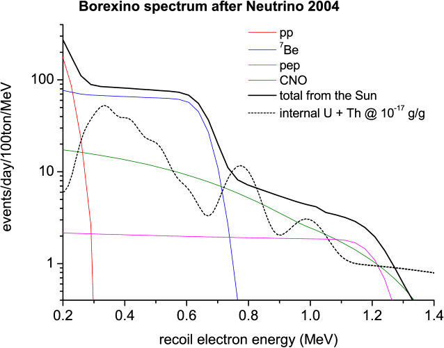
  Figure 12: Expected solar neutrino rates in Borexino. The solid line is the expected total neutrino spectrum between 0.2 and 1.4 MeV, based on the MSW LMA solution and BP04 [71]. The dotted line is the internal background from U and Th, assumed at a level of $10^{-17}$ g/g, shown as a reference. Other sources of background are not included.

  illustrates background from the U and Th chains if their concentrations are at $10^{-17}$ g/g and no additional cuts are applied. The background shown in Figure 12 can further be reduced by various cuts, including $\alpha\backslash\beta$ separation which is expected to reduce the alphas by more than a factor of 10. The U and Th concentrations are 10 times lower than our current limits, but consistent with recent data from KamLAND. If backgrounds are low enough to measure ⁷Be neutrinos to 5$\%$, the pep neutrinos should also be measurable, with a precision better than 10$\%$.

  Borexino and other experiments at Gran Sasso were placed under judicial sequestration following a small spill of scintillator in August 2002. The sequestration stopped all work underground. In the spring of 2003 a partial lifting of the sequestration was granted to permit mechanical construction of the detector to restart. However, the ban on fluid use remained in force, owing to the discovery of flaws in the drainage system. In June 2003 a special commissioner was appointed by the italian government to assume responsibility for repairing the laboratory infrastructure and restoring the laboratory to full operations. As of June 2004, the commissioner’s staff is still implementing the repairs. A full lifting of the sequestration is expected late this summer, two years after the incident. The first operations that will occur after the sequestration is lifted will be filling the detector with high purity water and studies of scintillator purification with the Counting Test Facility.

3.4.2 $pp$

Measurement of the $pp$ neutrino flux will require an experimental technique that allows very low radioactive backgrounds for energies $<300$ keV. In contrast to other low energy solar experiments done so far, the proposed experiments aim at measuring the full spectrum below 2 MeV, therefore including the fluxes from all the major sources in the Sun. Proposed $pp$ experiments fall in two classes: neutrino- electron scattering (ES) and charge current neutrino absorption (CC).

The ES proposals (CLEAN and HERON) have the advantage of promising very low internal backgrounds by virtue of the cleanliness of their detection media. Helium, as a superfluid at 50 mK, is completely free of any activity; Neon at 27 K can be ultra-purified. Neutrino-electron elastic scattering cross-sections are well known from electroweak theory, so ES experiments do not need to be calibrated with a neutrino source. CC experiments are attractive because they exclusively yield the electron flavor flux of ⁷Be neutrinos in particular, complementing the NC flavor content obtainable from present ES experiments such as Borexino and Kamland. Of course, measuring fluxes both via ES and CC reactions could allow a determination of the total active $pp$ neutrino flux independent of the mixing parameters.

Both types of experiments must be located deep underground to avoid backgrounds from muon spallation. CLEAN and HERON have very different approaches to rejection of gamma ray backgrounds. CLEAN would use the relatively dense liquid neon to absorb external gamma rays before they reach the inner fiducial region, then cut gamma ray events using position resolution. HERON would have sufficient position resolution to distinguish point sources (signal) from distributed sources (gamma rays).

The CC proposal (LENS) would use a target of Indium incorporated into organic scintillator. Because Indium emits a delayed gamma ray after neutrino absorption, coincidence techniques can be used to greatly reduce radioactive backgrounds, including bremstrahlung from Indium $\beta$-decay. The delayed coincidence signature distinguishes a neutrino event from background, and allows the simultaneous measurement of signal and background independently. Also, because the neutrino energy is entirely captured, the shape of the $pp$ and ⁷Be neutrino spectra may be directly measured. LENS has only a modest depth requirement ($>$ 2000 m.w.e.). For an accurate $pp$ neutrino measurement, the neutrino absorption cross- section must be calibrated using a MCi neutrino source, probably $\rm{}^{37}Ar$.

Figure 13 shows the expected reconstructed energy spectra from simulations of neutrino interactions and backgrounds in these experiments.

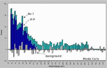
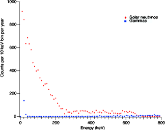
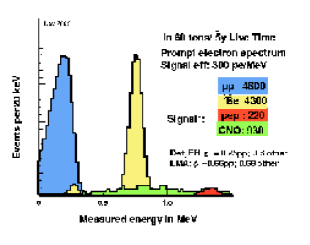
Figure 13: Simulations of reconstructed energy spectra for future low energy solar neutrino experiments. From top to bottom are the simulations for the HERON experiment, the CLEAN experiment, and the LENS experiment.

While the technical challenges of these experiments are of high order, there has been much progress in overcoming them. Below we detail some of the expectations for the precision of the different experiments, and some of the specific challenges and advantages of each method.

• HERON

  The estimates on the uncertainties for HERON are shown in Table 4, and have been made on the basis of extensive prototype experimentation on the particle detection properties of superfluid helium and on the wafer detector devices to be used in a full scale device. Also, detailed simulations of signal and background events from energy deposition to full event reconstruction in a full-scale detector design have been used. The detector is assumed to be at a depth of at least 4500 m.w.e., externally shielded, and residual backgrounds due to site environmental sources have been shown to be negligible. The dominant source of background are the materials of the cryostat and moderator; they have been taken for the copper cryostat: primordials and cosmogenics (as measured by double beta decay and dark matter experiments as well as by ICPMS and NAA measurements). For the moderator N2 : primordials, cosmogenics and anthropogenics from the Heidelberg LN2 extensive studies. Activity concentrations for plastics are taken from the large studies at SNO and KamLAND.

  Table 4: Uncertainties on $pp$ flux for HERON.

  	$pp$ uncert. (%)
  Threshold cut (Energy scale and $\sigma$)	1.25
  Fiducial volume	1.3
  Efficiency	1.5
  Signal/backgrounds separation fit	2.5
  Internal background	0.0
  Density uniformity of target vol.	0.0
  cross section	0.25
  Deadtime	0.04
  pp/7Be separation	0.25
  Total systematic (quadrature sum)	3.4
  Statistics ($pp$)	1.0
  Statistics (7Be)	1.5
  Total	3.5

  The energy threshold used to produce the numbers in Table 4 is set at 45 keV visible electron recoil energy and the energy resolution (FWHM) ranged from 3.2% at 600 keV to 10.3% at 45 keV. The absolute scale assumed at 2%, and the helium fiducial volume of 68 m³ with position resolution of $\sigma_{x}=1.62$ cm, $\sigma_{y}=1.54$ cm,and $\sigma_{z}=2.46$ cm. The signal and backgrounds can be separated by their distinct energy and spatial distributions both inside and outside the fiducial volumes, as well as the Earth orbital eccentricity variation of the signal neutrino flux. The superfluid helium itself is entirely free of any activity.

• CLEAN

  Table 5 summarizes the projected uncertainties for solar neutrino flux measurements with a 300 cm radius liquid neon detector (CLEAN), assuming both 1 year and 5 year runs. A fiducial volume defined by a 200 cm radial cut is assumed, for a total active mass of 40 tonnes. The detector is assumed to be at a depth of 6000 m water equivalent, where cosmic-ray induced backgrounds and related uncertainties are negligible. Dominant sources of backgrounds are assumed to be internal radioactivity, and radioactivity from the PMT glass found in certain commercially available phototubes (30 ppb uranium, thorium, 60 ppm potassium). Above the neutrino analysis threshold of 35 keV the fiducial volume cut is expected to remove essentially all background events from PMT activity. The total event rates for $pp$ and ⁷Be neutrino interactions are calculated assuming the current best-fit LMA solution, and SSM fluxes. Two analysis windows are defined: 35-300 keV for $pp$ events, and 300-800 keV for ⁷Be events. Fluxes are derived from the event rates in these windows. Uncertainties related to the neutrino mixing model are not considered.

  Table 5: Uncertainties on $pp$ and ⁷Be fluxes for CLEAN.

  	$pp$ uncert.		7Be uncert.
  	(%)		(%)
  	1 y	5 y	1 y	5 y
  Energy scale	0.34	0.34	0.87	0.87
  Fiducial volume	0.90	0.90	0.90	0.90
  Internal krypton	0.25	0.25	1.87	1.87
  External backgrounds	0.04	0.02	0.15	0.07
  7Be $\nu$’s	0.25	0.11	0	0
  Total systematic	1.03	1.00	2.26	2.25
  Statistics	0.86	0.38	2.87	1.28
  Total	1.34	1.07	3.65	2.59

  In Table 5, the absolute energy scale uncertainty is assumed to be 1%, and is assumed to be determined by deploying $\gamma$-ray calibration sources throughout the detector volume many times. The dominant uncertainty is expected to arise from the uncertainty in converting absolute $\gamma$-ray energies to electron energies with a Monte Carlo model. The uncertainty in the neutrino flux arising from the uncertainty on energy resolution is negligible.

  The dominant uncertainty on the measurement of the $pp$ flux is the uncertainty on the fiducial volume. If CLEAN can do $\sim$ 3 times better than SNO, then the uncertainty $\frac{\Delta R}{R}=0.3\%$, leading to less than a 1% uncertainty on volume. Doing as well as 0.3% will require source positioning to be accurate to 0.6 cm, and the positioning system will need to be able to reach nearly all positions within the detector volume.

  Internal background from Krypton, Uranium, and Thorium are expected to be small, and in the worst case (Krypton) known to 25%. These backgrounds will be measured by assaying the neon, or by measuring them in-situ with the PMT data.

  External backgrounds, dominated by PMT activity, will be removed primarily by the fiducial volume cut, and can be tested by deploying a very hot source exterior to the volume and counting the number of events which reconstruct inside. The fiducial volume cut is particularly effective because of the high density of liquid neon (1.2 g/cc). Position resolution in CLEAN is based on PMT hit pattern and timing, and is confirmed in detailed Monte Carlo simulations.

• LENS

  The following tables summarize preliminary estimates of precision expected in $pp$ and ⁷Be flux measurements in the LENS-Sol solar detector in conjunction with the LENS-Cal ³⁷Ar source calibration. The results are obtained for two different Indium target masses, 60 and 30 tons to illustrate the roles of statistical and systematic errors. The latter is set identical for both target masses. LENS is planned to have a modular detector architecture, thus the performance of the full-scale detector can be closely predicted from bench top tests of individual modules

  Table 6: Uncertainties on $pp$ and ⁷Be fluxes for LENS.

  	$pp$ uncert.		7Be uncert.
  	(%)		(%)
  	30 t	60 t	30 t	60 t
  Signal/Background Statistics	2.33	1.65	2.12	1.5
  Coincidence Detection Efficiency	0.7	0.70	0.70	0.70
  Number of Target Nuclei	0.3	0.3	0.3	0.3
  Cross Section (Q-value)	0.3	0.3	0.16	0.16
  Cross Section (G-T matrix element)	1.8	1.8	1.8	1.8
  Total Uncertainty	3.05	2.57	2.87	2.46

  The only correlated backgrounds to the triple coincidence arise from cosmogenic (p,n) reactions on Indium. These are expected to be about 5% of the solar signal at a depth of 1600 m.w.e., but will be vetoed by tagging the initiating cosmic. The triple-coincidence detection efficiency has been estimated through Monte Carlo simulation, and includes cuts on energy, time, and the In and In-free parts of the detector. For the $pp$ neutrinos the efficiency is expected to be $\sim$25%, and for ⁷Be neutrinos $\sim$80%. An experimental determination of the coincidence efficiency can be made by using a small surface detector and using cosmic-ray induced products, which can produce the same signals as the neutrino events. These measurements are expected to yield the uncertainty shown in Table 6.

  The segmentation of the detector will allow the fiducial volume to be determined by the dimensions of the detector, not on an offline-cut, and the uncertainty on the number of target nuclei will depend primarily on the chemical determination of the Indium content in the In-loaded liquid scintillator.

  To determine uncertainties associated with the cross section (knowledge of the Q-value as well as the matrix element) a 5-ton calibration detector and strong (2-MCi) ³⁷Ar source will be used.

3.5 Supporting Nuclear Physics Measurements

As described in Sections 3,3.2.1, and 3.2.5 comparison of the neutrino fluxes to the predictions of the Standard Solar Model allow us to search for both new astrophysics and new particle physics. To make the comparison meaningful, we would like for the precision of the predictions to be comparable to that of the measurements.

A global analysis of all solar experiments and KamLAND yields the total ⁸B solar neutrino flux with a precision of $\pm$ 4% [17]. We would therefore hope to reduce the uncertainties on the Standard Solar Model prediction to a level of 5% or smaller.

Recently, new measurements have been made of the C, N, O, Ne, and Ar abundances on the surface of the Sun [77]. The current uncertainty in solar composition (Z/X) leads to a large 8% and 20% uncertainty  [78, 79, 80] in the predicted ⁷Be and ⁸B solar neutrino flux, respectively, and therefore to improve the precision on the prediction, we need new measurements.

Nuclear inputs to the SSM, in particular the cross sections $S_{17}(0)$ and $S_{34}(0)$ , as defined by Adelberger et al. [81], need to be known with a precision better than 5%. High precision (3-5%) measurements of $S_{17}$ are now available from experiments using very different methods or experimental procedures [83, 84, 85, 86]. The mean of the modern direct measurements below the 630-keV $1^{+}$ resonance gives S₁₇(0) to 4%. Significant differences are apparent, however, between the indirect (Coulomb dissociation and heavy-ion transfer) and direct determinations of S₁₇(0), which merit further exploration—see Fig. 14. An additional high-precision direct measurement is in progress.

The most recent evaluation of $S_{34}(0)$ was performed in 1999 by Adelberger et al. [81] and unfortunately no new data on $S_{34}(0)$ were reported in the intervening time period. A 13% discrepancy between the low and high values of $S_{34}(0)$ was found by Adelberger et al., who quote $S_{34}(0)$ with a 9% accuracy. Additional direct experimental measurements are necessary to reduce the uncertainty on S₃₄(0) below 5%.

As a particular example we note that the precision value measured by the Seattle group $S_{17}(0)$ = 22.1 $\pm$ 0.6 [83], together with the larger value of $S_{34}(0)$ = 572 $\pm$ 26 eV-b deduced from ⁷Be activity measurements [81, 87] yield a predicted total ⁸B neutrino flux that is 20% larger than measured by SNO. The smaller value of $S_{34}(0)$ = 507 $\pm$ 16 eV-b [81] on the other hand reduces the discrepancy to 9%. Currently the ⁸B solar neutrino flux is predicted with 23% uncertainty [71] with the main uncertainty due to the solar composition (Z), as discussed above. Such a discrepancy can only be considered significant with an improved precision of the prediction of the SSM, and it may for example provide evidence of oscillation into sterile neutrino.

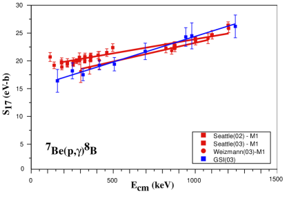
Figure 14: A comparison of a selection of the recent Seattle(02) [83], Weizmann(03) [84], and GSI [85, 86] data. An M1 contribution due to the resonance at 632 keV is subtracted from the direct capture data. The slope of the indirect Coulomb breakup results appear to disagree somewhat with that of the direct cross section measurements. A detailed theoretical re-evaluation is in progress.

3.6 Other Physics with Solar Neutrino Detectors

Nearly all detectors described in the previous sections are capable of doing other physics besides solar neutrino observations. The detection of neutrinos from supernovae can be done particularly well by large-scale water Cerenkov experiments, but also by many of the other detectors as well. The detection of the constituents of dark matter are an explicit goal of some of the $pp$ experiments. In addition, many of these experiments can serve as antineutrino detectors as well, perhaps able to observe (or limit) the flux of geoneutrinos originating within the Earth. Although the focus of this report is solar and atmospheric neutrino detection, we do want to emphasize the fact that the detectors themselves have a justification that includes a range of physics outside that focus.

4 Atmospheric Neutrino Experiments

The study of atmospheric neutrinos—neutrinos produced by the interactions of cosmic rays with the atmosphere—should have been straightforward. While the detection of such neutrinos was by themselves interesting, and while some envisioned the possibilities for these neutrinos to help us discover leptonic flavor transformation, the primary physics we expected to learn was how cosmic rays interact in the atmosphere, what the fluxes of different types of neutrinos were, and what the neutrino energy spectra were.

It was clear almost from the outset, however, that something was wrong. The two largest experiments capable of detecting atmospheric neutrinos—IMB [2, 3] and Kamiokande [4]—both saw that the ratio of $\nu_{\mu}$’s to $\nu_{e}$’s was significantly different than expectations. One possibility which explained such an observation was that upward $\nu_{\mu}$’s were disappearing due to neutrino oscillations, but other possibilities were still considered. In addition, if oscillations were the explanation, the data indicated that the mixing between the neutrino mass states was maximal or nearly so—something which contradicted the prejudices based on the small quark mixing angles.

It was not until 1998, when the Super-Kamiokande collaboration published a high statistics plot of the number of detected neutrinos as a function of zenith angle, that the oscillation hypothesis was clearly demonstrated [37]. Figure 15 shows an updated

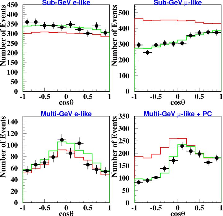
Figure 15: Zenith angle distributions for atmospheric neutrino interactions in Super-Kamiokande [115].

version of the $\cos{\theta_{z}}$ distribution for both $\nu_{e}$’s and $\nu_{\mu}$’s, compared to the oscillation hypothesis. We can see that the fit to the data for an oscillation of $\nu_{\mu}$’s is extremely good, and that the null hypothesis of no transformation is not possible. Other experiments—MACRO [39] and Soudan 2 [40]—using very different methods subsequently confirmed Super-Kamiokande’s measurements. Fig. 16 [88] shows the summary of the results on the mixing parameters determined by all the atmospheric experiments.

In the following sections, we describe both the role that future atmospheric experiments can play in testing the three-flavor oscillation model, as well as the potentially critical role they may play in resolving the mass hierarchy. We finish with a short discussion of some of the non-oscillation physics which can be done with these experiments.

4.1 Testing the Neutrino Oscillation Model

As discussed in Section 3.2, our model of neutrino flavor transformation requires the addition of (at least) seven new fundamental parameters to the Standard Model of particle physics: three mixing angles, a complex phase, and three neutrino masses. With these new parameters, the Model predicts all transformation phenomena regardless of energy, baseline, lepton number, flavor, or intervening matter. To test the Model, we therefore need to measure the parameters and compare them across experimental regimes such as energy, baseline, etc., verify some of the explicit predictions of the Model such as the oscillatory nature of the transformation, look for the predicted sub-dominant effects, and search for some of the possible non-Standard Model transformation signatures.

The enormous experimental regime covered by the atmospheric measurements means that they are particularly sensitive tests, and in many ways the atmospheric sector is far ahead of the solar sector in verifying some of the finer details of the transformation model.

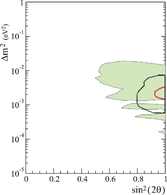
Figure 16: The shaded region shows the allowed region from the latest Soudan 2 results; the outer unfilled black contour shows the allowed region from MACRO upward-going muons; and the inner solid red contour shows the results from Super-Kamiokande.. Figure taken from Ref. [88].

4.1.1 Precision Measurements in the (2,3) Sector

The wide dynamic range of neutrino energies and baselines in the atmospheric sector mean that atmospheric experiments provide their own tests of the oscillation model—the predictions can be shown to hold across all the accessible experimental regimes. Improved precision in these experiments thus provide interesting tests of the oscillation model even in the absence of other experimental approaches.

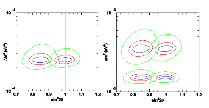
Figure 17: Allowed regions showing expected sensitivity to dominant oscillation parameters for Super-Kamiokande (or similar water Cerenkov detector). Each set of contours corresponds to a particular assumption of true oscillation parameters. For each set of contours, the outer (green) one represents a 113 kton-year exposure (5 years of SK); the red represents 450 kton-years (20 years of SK); the inner (blue) one represents 1800 kton-years (80 years of SK). Figures taken from Ref. [100].

Figure 17 shows the expected sensitivity to the dominant oscillation parameters from atmospheric neutrinos, for various exposures of Super-Kamiokande and various assumed true values of the parameters. These results assume use of an analysis similar to the high resolution L/E analysis of Ref. [90] (and see Section 4.1.2). The size of the regions shrink with the square root of the exposure, as expected, but it is clear from the plot that ultimate sensitivity to $\Delta m^{2}$ depends also on the actual values of the parameters. Of course, the sensitivities of the next generation of long baseline accelerator experiments are competitive with the measurements made by the atmospheric experiments.

The first long baseline accelerator neutrino experiment K2K [55, 89] has confirmed this picture, thus providing the first test of the oscillation model in the atmospheric sector. Further data from Super-K, K2K and MINOS will enable more precise determination of these two-flavor mixing parameters, and comparison of these experiments provide more stringent tests of the three-flavor oscillation model.

4.1.2 Direct Observations of the Oscillatory Behavior

One of the most explicit tests of the oscillation model is to observe the oscillations themselves—up until recently, no measurement of flavor transformation could show the expected oscillation with baseline and energy (L/E) which is a fundamental prediction of the model. That has changed now that the Super-Kamiokande (SK) collaboration has shown an “oscillation dip” in the $L/E-$dependence, of the $\mu-$like atmospheric neutrino events (see Fig. 18, Ref.  [90]) , $L$ and $E$ being the distance traveled by neutrinos and the neutrino energy. As is well known, the SK atmospheric neutrino data are best described in terms of dominant two-neutrino $\nu_{\mu}\rightarrow\nu_{\tau}$ ($\bar{\nu}_{\mu}\rightarrow\bar{\nu}_{\tau}$) vacuum oscillations with maximal mixing, $\sin^{2}2\theta_{23}\cong 1$ with $\Delta m^{2}_{23}$ being the neutrino mass squared difference responsible for the atmospheric $\nu_{\mu}$ and $\bar{\nu}_{\mu}$ oscillations. This result represents the first ever observation of a direct oscillatory dependence of $L/E$.

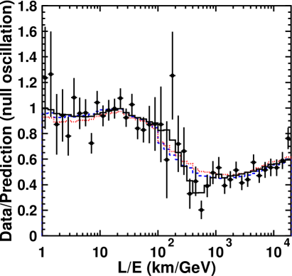
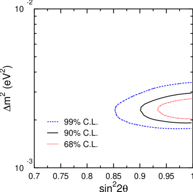
Figure 18: Left: ratio of data to Monte Carlo events without neutrino oscillation (points) as a function of reconstructed L/E, with best-fit expectation for two-flavor $\nu_{\mu}\rightarrow\nu_{\tau}$ oscillations (solid line). The dashed and dotted lines show disfavored decay and decoherence models. Right: corresponding allowed oscillation parameter regions. Figures taken from Ref. [90].

Future, larger-scale experiments such as UNO [33] or Hyper-Kamiokande [72] should be able to see this kind of effect with far greater signficance. Figure 19 shows the oscillation pattern which could be observed by the UNO detector.

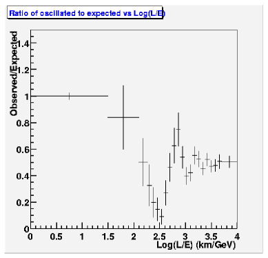
Figure 19: Simulated oscillation pattern observable by UNO [33].

4.1.3 Searches for Sub-Dominant Effects

The $\nu_{\mu}\rightarrow\nu_{e}$ ($\bar{\nu}_{\mu}\rightarrow\bar{\nu}_{e}$) and $\nu_{e}\rightarrow\nu_{\mu(\tau)}$ ($\bar{\nu}_{e}\rightarrow\bar{\nu}_{\mu(\tau)}$) subdominant oscillations of atmospheric neutrinos should exist and their effects could be observable if genuine three-flavor-neutrino mixing takes place in vacuum, i.e., if $\sin^{2}2\theta_{13}\neq 0$, and if $\sin^{2}2\theta_{13}$ is sufficiently large [102, 103, 104]. The subdominant $\Delta m^{2}_{21}$ effects depend crucially on the value of $\theta_{23}$, i.e. whether it is larger or smaller than 45^o. These effects, as those associated with $\delta$ (CP-violating phase), only show up at sub-GeV energies, for which the oscillation length due to $\Delta m^{2}_{21}$ becomes comparable to the typical distances for atmospheric neutrinos crossing the Earth.

In addition, if $\sin^{2}2\theta_{13}$ is sufficiently large, subdominant effects should exist in the multi-GeV range too. In this case, $\nu_{\mu}\rightarrow\nu_{e}$ ($\bar{\nu}_{\mu}\rightarrow\bar{\nu}_{e}$) and $\nu_{e}\rightarrow\nu_{\mu(\tau)}$ ($\bar{\nu}_{e}\rightarrow\bar{\nu}_{\mu(\tau)}$) transitions of atmospheric neutrinos are amplified by Earth matter effects. But matter affects neutrinos and antineutrinos differently, and thus the study of these subdominant effects can provide unique information (see Section 4.2).

The analytic analyses of references [105, 106] imply that in the case under study the effects of the $\nu_{\mu}\rightarrow\nu_{e}$, $\bar{\nu}_{\mu}\rightarrow\bar{\nu}_{e}$, and $\nu_{e}\rightarrow\nu_{\mu(\tau)}$, $\bar{\nu}_{e}\rightarrow\bar{\nu}_{\mu(\tau)}$, oscillations i) increase with the increase of $s^{2}_{23}$ and are maximal for the largest allowed value of $s^{2}_{23}$, ii) should be considerably larger in the multi-GeV samples of events than in the sub-GeV samples, iii) in the case of the multi-GeV samples, they lead to an increase of the rate of $e-$like events and to a slight decrease of the $\mu-$like event rate. This analysis suggests that in water-Čerenkov detectors, the quantity most sensitive to the effects of the oscillations of interest should be the ratio of the $\mu-$like and $e-$like multi-GeV events (or event rates), $N_{\mu}/N_{e}$.

The magnitudes of the effects we are interested in depend also on the 2-neutrino oscillation probabilities. In the case of oscillations in vacuum we have $P_{2\nu}(\mbox{$\Delta m^{2}_{23}$},\theta_{13};E,\theta_{n})=\bar{P}_{2\nu}(\mbox{$\Delta m^{2}_{23}$},\theta_{13};E,\theta_{n})\sim\sin^{2}2\theta_{13}$. Given the existing limits on $\sin^{2}2\theta_{13}$, the probabilities $P_{2\nu}$ and $\bar{P}_{2\nu}$ cannot be large if the oscillations take place in vacuum. However, $P_{2\nu}$ or $\bar{P}_{2\nu}$ can be strongly enhanced by the Earth matter effects (see Section 4.2).

For small $\theta_{13}$ the only effect able to discriminate the octant of $\theta_{23}$ is associated with subdominant $\Delta m^{2}_{21}$ oscillations which are neglected in the hierarchical approximation used in the standard three-neutrino oscillation analysis. This effect can be understood in terms of approximate analytical expressions developed in Ref. [42, 43].

The sensitivity for future experiments can be determined by constructing a $\chi^{2}$ which is a function of the oscillation parameters and the data (see Ref. [43]), and evaluating the difference in $\chi^{2}$ for “false” and “true” $\theta_{23}$ minima. Figure 20 summarizes the results of ref [43]: it shows that unless $\theta_{23}$ is very close to maximal mixing, there is good discrimination power from a high statistics future atmospheric neutrino experiment. This effect is much increased if the theoretical uncertainties on the atmospheric fluxes and the interaction cross section as well as the experimental systematic uncertainties are reduced.

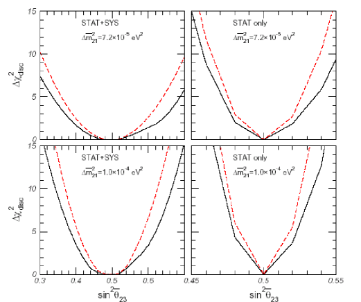
Figure 20: $\Delta\chi^{2}$ between the “false” and “true” $\theta_{23}$ minima for future ATM (+OTHERS) experiments as a function of the simulated $\overline{\sin^{2}\theta_{23}}$. The upper (lower) panels are for the simulated parameters : $\overline{\Delta m^{2}_{21}}=7.2\;(10)\;\times 10^{-5}\;{\rm eV}^{2}$, $\overline{\tan^{2}\theta_{21}}=0.42$, $\overline{\Delta m^{2}_{31}}=2.2\times 10^{-3}\;{\rm eV}^{2}$ $\overline{\sin^{2}\theta_{13}}=0$, $\overline{\delta}=0$. The left panel assumes 20 times SK statistics but the same theoretical and systematic errors. In the right panel, no theoretical and systematic errors are included.

4.1.4 Other Transformation Hypotheses

As discussed in Section 3.2.1, any new physics which leads to differences in neutrino propagation may lead to neutrino transformation effects. Although these effects are now all excluded as the dominant source of flavor transformation in both the solar and atmospheric sectors, in the atmospheric sector they are severely restricted even at the sub-dominant level.

The atmospheric neutrino data span several decades in neutrino energy and distance. As a consequence it is very sensitive to these forms of new physics. The question arises, therefore, at what point the possible presence of these forms of new physics, even if sub-dominant, may affect the derived ranges of masses and mixing from the oscillation analysis of the atmospheric data. Or in other words, to what level our present determination of the neutrino masses and mixing is robust under the presence of phenomenologically allowed new physics effects.

This question has been recently answered in Ref. [53] in which a global analysis of the atmospheric is performed with $\nu_{\mu}\to\nu_{\tau}$ transitions driven by neutrino masses and mixing in the presence of these forms of new physics.

In general when both neutrino masses and mixing and some of these generic forms of new physics coexist, the evolution of the neutrinos is governed by the equation

$$\mathbf{H}_{\pm}\equiv\frac{\Delta m^{2}}{4E}{\mathbf{U}_{\theta}}\left(\begin{array}[]{cc}-1&~{}0\\ \hphantom{-}0&~{}1\end{array}\right){\mathbf{U}_{\theta}^{\dagger}}+\sigma_{n}^{\pm}\frac{{\Delta\delta_{n}}\,{E^{n}}}{2}{\mathbf{U}_{\xi_{n}}}\left(\begin{array}[]{cc}-1&~{}0\\ \hphantom{-}0&~{}1\end{array}\right){\mathbf{U}_{\xi_{n}}^{\dagger}}\;,$$ (6)

where $\Delta m^{2}$ is the mass–squared difference between the two neutrino mass eigenstates, $\sigma_{n}^{\pm}$ accounts for a possible relative sign of the NP effects between neutrinos and antineutrinos and $\Delta\delta_{n}$ parametrizes the size of the NP terms. $\mathbf{U}_{\theta}$ ($\mathbf{U}_{\xi_{n},\pm\eta_{n}}$) is the rotation matrices between the flavor states and the mass eigenstates (NP eigenstates). In general a non-vanishing relative phase $\eta_{n}$ is also possible.

For Violation of Equivalence Principle

$${\Delta\delta_{1}=2|\phi|(\gamma_{1}-\gamma_{2})\equiv 2|\phi|\Delta\gamma}\,,\qquad\sigma_{1}^{+}=\sigma_{1}^{-}\,.$$

For Violation of Lorentz Invariance:

$${\Delta\delta_{1}=(v_{1}-v_{2})\equiv\,\delta v}\,,\qquad\sigma_{1}^{+}=\sigma_{1}^{-}\,.$$

For Coupling to a space-time torsion field

$${\Delta\delta_{0}=Q(k_{1}-k_{2})\equiv Q\,\delta k}\,,\qquad\sigma_{0}^{+}=\sigma_{0}^{-}\,.$$

For Violation of Lorentz Invariance via CPT violation

$${\Delta\delta_{0}=b_{1}-b_{2}\equiv\delta b}\,,\qquad\sigma_{0}^{+}=-\sigma_{0}^{-}$$

For NSNI

$${\Delta\delta_{0}}=2\sqrt{2}\,G_{F}\,N_{f}(\vec{r}){\sqrt{\varepsilon_{\mu\tau}^{2}+\frac{(\varepsilon_{\mu\mu}-\varepsilon_{\tau\tau})^{2}}{4}}}\qquad{\sin^{2}2\xi=\frac{\varepsilon_{\mu\tau}}{\sqrt{\varepsilon_{\mu\tau}^{2}+\frac{(\varepsilon_{\mu\mu}-\varepsilon_{\tau\tau})^{2}}{4}}}}\qquad\sigma_{0}^{+}=-\sigma_{0}^{-}$$

In all these scenarios the oscillation probabilities can be written as:

$$P_{\nu_{\mu}\to\nu_{\mu}}=1-P_{\nu_{\mu}\to\nu_{\tau}}=1-\sin^{2}2\Theta\,\sin^{2}\left(\frac{\Delta m^{2}L}{4E}\,\mathcal{R}\right)\,.$$ (7)

where the correction to the $\Delta m^{2}$-OSC wavelength, $\mathcal{R}$, and to the global mixing angle, $\Theta$, verify

$${\mathcal{R}}\cos 2\Theta\, =\cos 2\theta+R_{n}\,\cos 2\xi_{n}\,,$$ (8)

$${\mathcal{R}}\sin 2\Theta\ =|\sin 2\theta+R_{n}\,\sin 2\xi_{n}\,e^{i\eta_{n}}|\,,$$ (9)

with $R_{n}$ being the ratio between the NP–induced and $\Delta m^{2}$–induced contributions to the oscillation wavelength. For $P_{\bar{\nu}_{\mu}\to\bar{\nu}_{\mu}}$ the same expressions hold with the exchange $\sigma_{n}^{+}\to\sigma_{n}^{-}$ and $\eta_{n}\to-\eta_{n}$.

Ther results of the analysis of the present atmospheric data is shown in Fig. 21 and  22.

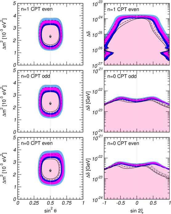
Figure 21: Allowed parameter regions for the analysis of atmospheric and K2K data in presence of $\nu_{\mu}\to\nu_{\tau}$ oscillations and different NP effects as labeled in the figure. The different contours correspond to the allowed regions at 90%, 95%, 99% and $3\sigma$ CL. The filled areas in the left panels show the projected two-dimensional allowed region on the oscillation parameters $\Delta m^{2}$–$\sin^{2}\theta$ plane. The best fit point is marked with a star. We also show the lines corresponding to the contours in the absence of new physics and mark with a triangle the position of the best fit point. The regions on the right panels show the allowed values for the parameters characterizing the strength and mixing of the NP. The full regions corresponds to arbitrary values of the phase $\eta_{n}$ while the lines correspond to the case $\eta_{n}\in\{0,\,\pi\}$.

The figure demonstrates that the data does not show any evidence of presence of NP even as a sub-dominant effect and the robustness of the allowed ranges of mass and mixing derived from the analysis of atmospheric and K2K data under the presence of these generic NP effects. Thus the analysis allow us to derive well-defined upper bounds on the NP strength. At 95% CL

$$|\delta v|\leq 8.1\times 10^{-25}$$

$$|\phi\,\Delta\gamma|\leq 4.0\times 10^{-25}$$

$$|\delta b|\leq 3.2\times 10^{-23}$$

$$|Q\,\delta k|\leq 4.0\times 10^{-23}$$

$$|\varepsilon_{\mu\mu}-\varepsilon_{\tau\tau}|\leq 0.013~{}$$

$$|\varepsilon_{\mu\tau}|\leq 0.034~{}$$

These limits are among the strongest constraints on these forms of NP.

Next we illustrate the attainable sensitivity at a future atmospheric neutrino experiment. In order to show this we have assumed a SK-like detector with 20 times the present SK statistics with the same theoretical and systematic uncertainties as SK. The results are shown in Figs. 23 and  24. In Fig 23 we have assumed that the observed rates will correspond to the present SK data. The figure illustrates that within the fluctuations in the existing data there is still room for NP. In Fig 24 we have assumed that the observed rates will correspond to the present best fit point for pure $\Delta m^{2}$ oscillations. The figure illustrates the possible improvement in the constraints on the NP strength due to the improved statistics.

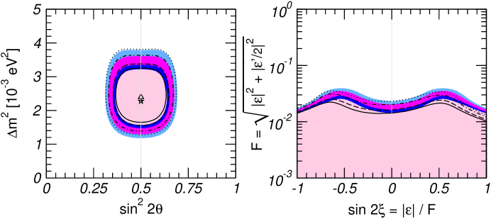
Figure 22: Same as Fig. 21 for the case of $\Delta m^{2}$-OSC+NSI. For the sake of concretness we have assumed NSI to $d$-quarks

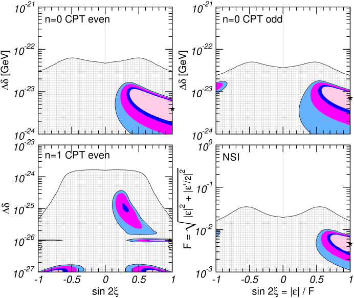
Figure 23: Allowed regions for the NP parameters for a future atmospheric neutrino experiment with 20 SK exposure and observed rates corresponding to the present SK data. The filled contours show the allowed region at 90%, 95%, 99% and $3\sigma$ CL. The hatched area is the presently excluded region at $3\sigma$.

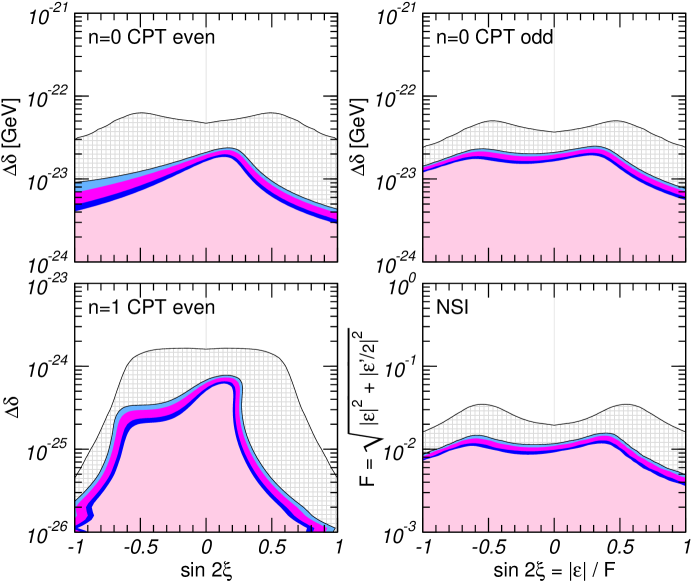
Figure 24: Allowed regions for the NP parameters for a future atmospheric neutrino experiment with 20 SK exposure and observed rates corresponding to the simulated $\Delta m^{2}$ oscillation best fit point. The filled contours show the allowed region at 90%, 95%, 99% and $3\sigma$ CL. The hatched area is the presently excluded region at $3\sigma$.

where the correction to the $\Delta m^{2}$-OSC wavelength, $\mathcal{R}$, and to the global mixing angle, $\Theta$, verify

$${\mathcal{R}}\cos 2\Theta\, =\cos 2\theta+R_{n}\,\cos 2\xi_{n}\,,$$ (10)

$${\mathcal{R}}\sin 2\Theta\ =|\sin 2\theta+R_{n}\,\sin 2\xi_{n}\,e^{i\eta_{n}}|\,,$$ (11)

with $R_{n}$ being the ratio between the NP–induced and $\Delta m^{2}$–induced contributions to the oscillation wavelength. For $P_{\bar{\nu}_{\mu}\to\bar{\nu}_{\mu}}$ the same expressions hold with the exchange $\sigma_{n}^{+}\to\sigma_{n}^{-}$ and $\eta_{n}\to-\eta_{n}$.

A more recent analysis [101], which included the effects of all three flavors found that non-standard interactions could play a role as large as Standard Model oscillations. If so, the mixing angle $\theta_{23}$ could be non-maximal, and $\Delta m_{23}^{2}$ somewhat higher than its present value.

4.2 The Matter Effect and the Mass Hierarchy

If $\sin^{2}\theta_{13}\neq 0$, the Earth matter effects can resonantly enhance either the $\nu_{\mu}\rightarrow\nu_{e}$ and $\nu_{e}\rightarrow\nu_{\mu}$, or the $\bar{\nu}_{\mu}\rightarrow\bar{\nu}_{e}$ and $\bar{\nu}_{e}\rightarrow\bar{\nu}_{\mu}$ transitions, depending on the sign of $\Delta m^{2}_{23}$. For $\mbox{$\Delta m^{2}_{23}$}>0$, the $\nu_{\mu}\rightarrow\nu_{e}$ and $\nu_{e}\rightarrow\nu_{\mu}$ transitions in the Earth lead to a reduction of the rate of the multi-GeV $\mu^{-}$ events, observable in detectors with charge discrimination, with respect to the case of absence of these transitions [102, 106, 104, 107]. If $\mbox{$\Delta m^{2}_{23}$}<0$, the $\mu^{+}$ event rate will be reduced. Correspondingly, as an observable which is sensitive to the Earth matter effects, and thus to the value of $\sin^{2}\theta_{13}$ and the sign of $\Delta m^{2}_{23}$, as well as to $\sin^{2}\theta_{23}$, we can consider the nadir-angle distributions of the $N(\mu^{-})-N(\mu^{+})$ asymmetry of the multi-GeV $\mu^{-}$ and $\mu^{+}$ event rates.

We note that atmospheric neutrino experiments are the only method other than long baseline experiments of determining the mass hierarchy, and for some values of the mixing parameters, they may be the only method.

In a water-Cerenkov detector the distinction between neutrino and antineutrino events is not possible (on an event-by-event basis), and in principle determining the type of neutrino mass hierarchy does not seem feasible. However, due to the difference of cross sections for neutrinos and antineutrinos, approximately 2/3 of the total rate of the $\mu-$like and $e-$like multi-GeV atmospheric neutrino events in a water-Cerenkov detector, i.e., $\sim 2N_{\mu}/3$ and $\sim 2N_{e}/3$, are due to neutrinos $\nu_{\mu}$ and $\nu_{e}$, respectively, while the remaining $\sim 1/3$ of the multi-GeV event rates, i.e., $\sim N_{\mu}/3$ and $\sim N_{e}/3$, are produced by antineutrinos $\bar{\nu}_{\mu}$ and $\bar{\nu}_{e}$. This implies that the Earth matter effects in the multi-GeV samples of $\mu-$like events will be smaller and that of $e-$like will be larger if $\mbox{$\Delta m^{2}_{23}$}>0$, i.e., if the neutrino mass spectrum is with normal hierarchy, than if $\mbox{$\Delta m^{2}_{23}$}<0$ and the spectrum is with inverted hierarchy. Thus, the ratio $N_{\mu}/N_{e}$ of the multi-GeV $\mu-$like and $e-$like event rates measured in the SK experiment could be sensitive, in principle, to the type of the neutrino mass spectrum.

It follows from the simple analysis of reference [108] that Earth matter effects can amplify $P_{2\nu}$ significantly when the neutrinos cross only the mantle i) for $E\sim(5-10)$ GeV, i.e., in the multi-GeV range of neutrino energies, and ii) only for sufficiently long neutrino paths in the mantle, i.e., for $\cos\theta_{n}\mathrel{\hbox to0.0pt{\raise 2.20013pt\hbox{$>$}\hss}{\lower 2.20013pt\hbox{$\sim$}}}0.4$. The magnitude of the matter effects in the ratio $N_{\mu}/N_{e}$ of interest increases with increasing $\sin^{2}\theta_{13}$. The same conclusions are valid for the antineutrino oscillation probability $\bar{P}_{2\nu}$ in the case of $\mbox{$\Delta m^{2}_{23}$}<0$. As a consequence, the ideal situation for distinguishing the type of mass hierarchy would be a detector with charge discrimination, such that neutrino interactions can be distinguished from those due to antineutrinos.

In the case of atmospheric neutrinos crossing the Earth core, new resonant effects become apparent. For $\sin^{2}\theta_{13}<0.05$ and $\mbox{$\Delta m^{2}_{23}$}>0$, we can have $P_{2\nu}\cong 1$ only due to the effect of maximal constructive interference between the amplitudes of the the $\nu_{e}\rightarrow\nu^{\prime}_{\tau}$ transitions in the Earth mantle and in the Earth core [102, 107, 109]. The effect differs from the MSW effect [102] and the resonances happen at lower energies, between the resonance energies corresponding to the density in the mantle and that of the core. The mantle-core enhancement effect is caused by the existence (for a given neutrino trajectory through the Earth core) of points of resonance-like total neutrino conversion, $P_{2\nu}=1$, in the corresponding space of neutrino oscillation parameters [107, 109]. The location of these points determines the regions where $P_{2\nu}$ is large, $P_{2\nu}\mathrel{\hbox to0.0pt{\raise 2.20013pt\hbox{$>$}\hss}{\lower 2.20013pt\hbox{$\sim$}}}0.5$. These regions vary slowly with the nadir angle; they are remarkably wide in the nadir angle and are rather wide in the neutrino energy [107], so that the transitions of interest produce noticeable effects: we have $\delta E/E\cong 0.3$ for the values of $\sin^{2}\theta_{13}$ of interest.

The effects of the mantle-core enhancement of $P_{2\nu}$ (or $\bar{P}_{2\nu}$) increase rapidly with $\sin^{2}\theta_{13}$ as long as $\sin^{2}\theta_{13}\mathrel{\hbox to0.0pt{\raise 2.20013pt\hbox{$<$}\hss}{\lower 2.20013pt\hbox{$\sim$}}}0.01$, and should exhibit a rather weak dependence on $\sin^{2}\theta_{13}$ for $0.01\mathrel{\hbox to0.0pt{\raise 2.20013pt\hbox{$<$}\hss}{\lower 2.20013pt\hbox{$\sim$}}}\sin^{2}\theta_{13}<0.05$. If 3-neutrino oscillations of atmospheric neutrinos take place, the magnitude of the matter effects in the multi-GeV $e-$like and $\mu-$like event samples, produced by neutrinos crossing the Earth core, should be larger than in the event samples due to neutrinos crossing only the Earth mantle (but not the core). This is a consequence of the fact that in the energy range of interest the atmospheric neutrino fluxes decrease rather rapidly with energy (approximately as $E^{-2.7}$), while the neutrino interaction cross section rises only linearly with $E$, and that the maximum of $P_{2\nu}$ (or $\bar{P}_{2\nu}$) due to the these new resonance-like effects takes place at approximately one half the energy than that due to the MSW effect for neutrinos crossing only the Earth mantle (e.g., at $E\cong(4.2-4.7)~{}{\rm GeV}$ and $E\cong 10~{}{\rm GeV}$, respectively, for $\mbox{$\Delta m^{2}_{23}$}=3\times 10^{-3}~{}{\rm eV^{2}}$).

Thus, summarizing, from the study of the Earth matter effects on atmospheric neutrinos one can conclude that: i) the medium effects, which discriminate between neutrino and antineutrino propagation, can help to determine the sign of the atmospheric $\Delta m^{2}_{23}$ [95]; ii) for $\sin\theta_{13}=0$ electron neutrinos decouple from the oscillations of the atmospheric neutrinos in matter, whereas they mix with the third (heaviest) mass eigenstate neutrino and take part in the atmospheric neutrino oscillations if $\sin\theta_{13}\not=0$, although their mixing with the first (lightest) mass eigenstate neutrino still vanishes; iii) non-resonant medium effects are already apparent in the sub-dominant channels $\nu_{e}\rightarrow\nu_{\mu}$ and $\bar{\nu}_{e}\rightarrow\bar{\nu}_{\mu}$, for baselines $L\sim 3000$ km, in both the mixing and oscillation phase shift (see also refs. [108, 96]); iv) in order for the medium effects in the muon neutrino survival probability to be observable, the resonant MSW effect in the $\nu_{e(\mu)}\rightarrow\nu_{\mu(e)}$ or $\bar{\nu}_{e(\mu)}\rightarrow\bar{\nu}_{\mu(e)}$ transitions must be operational, which requires baselines larger than $L\sim 7000$ km, the optimal baseline being a function of the value of $\sin\theta_{13}$; v) taking into account the initial atmospheric $\nu_{\mu}$, $\bar{\nu}_{\mu}$, and $\nu_{e}$, $\bar{\nu}_{e}$ fluxes and the relevant charged current neutrino-nucleon deep inelastic scattering cross-sections, it was shown that the matter-induced CPT-odd [110] and CP-odd [95, 108, 96] asymmetries are observable.

Observables: Water Cerenkov Detectors       

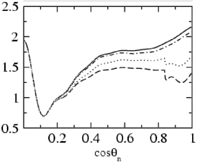
Figure 25: The dependence on $\cos\theta_{n}$ of the ratios of the multi-GeV $\mu^{-}$ and $e^{-}$ like events (or event rates), integrated over the neutrino energy in the interval $E=(2.0-10.0)$ GeV, in the cases i) of 2-neutrino $\nu_{\mu}\rightarrow\nu_{\tau}$ and $\bar{\nu}_{\mu}\rightarrow\bar{\nu}_{\tau}$ oscillations in vacuum and no $\nu_{e}$ and $\bar{\nu}_{e}$ oscillations, $N^{2\nu}_{\mu}/N^{0}_{e}$ (solid lines), ii) 3-neutrino oscillations in vacuum of $\nu_{\mu}$, $\bar{\nu}_{\mu}$, $\nu_{e}$ and $\bar{\nu}_{e}$, $(N^{3\nu}_{\mu}/N^{3\nu}_{e})_{vac}$ (dash-dotted lines), iii) 3-neutrino oscillations of $\nu_{\mu}$, $\bar{\nu}_{\mu}$ $\nu_{e}$ and $\bar{\nu}_{e}$ in the Earth and neutrino mass spectrum with normal hierarchy $(N^{3\nu}_{\mu}/N^{3\nu}_{e})_{\rm NH}$ (dashed lines), or with inverted hierarchy, $(N^{3\nu}_{\mu}/N^{3\nu}_{e})_{\rm IH}$ (dotted lines). The results shown are for $|\mbox{$\Delta m^{2}_{23}$}|=3\times 10^{-3}~{}{\rm eV^{2}}$, $\sin^{2}\theta_{23}=~{}0.64$, and $\sin^{2}2\theta_{13}=0.05$. Figure taken from Ref. [111].

The predicted dependence on $\cos\theta_{n}$ of the ratios of the multi-GeV $\mu-$ and $e-$ like events (or event rates), integrated over the neutrino energy from the interval $E=(2.0-10.0)$ GeV, for various cases, and for a particular choice of parameters, are shown in Fig. 25 [111].

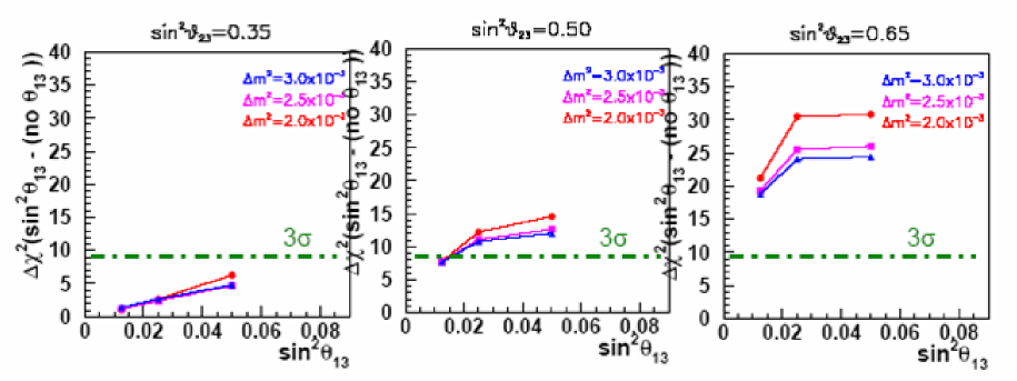
Figure 26: Statistical significance of a non-zero $\sin^{2}\theta_{13}$ with a water-Cerenkov detector with an exposure of 450 kton yrs (assuming normal hierarchy, i.e., $\mbox{$\Delta m^{2}_{23}$}>0$) for $\mbox{$\Delta m^{2}_{23}$}=2.0\times 10^{-3}~{}{\rm eV}^{2}~{}{(\rm red~{}line;)}~{}2.5\times 10^{-3}~{}{\rm eV}^{2}~{}{\rm(pink~{}line);and}~{}3.0\times 10^{-3}~{}{\rm eV}^{2}~{}{\rm(blue~{}line)}$ and $\sin^{2}\theta_{23}=0.35~{}{\rm(left~{}panel);}~{}0.50~{}{\rm(middle~{}panel)~{}and}~{}0.65~{}{\rm(right~{}panel)}$. Figure taken from Ref. [100].

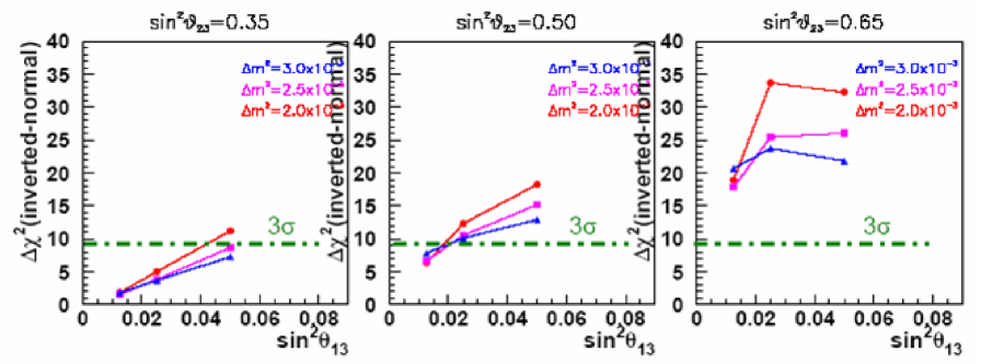
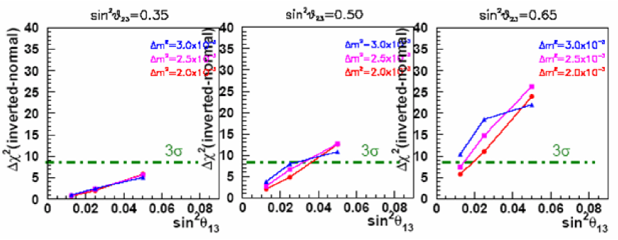
Figure 27: Statistical significance for measuring the sign of $\Delta m^{2}_{23}$ for an exposure of 1.8 Mton yrs if the true hierarchy turns out to be normal (upper plots) or inverted (lower plots), for different values of $|\mbox{$\Delta m^{2}_{23}$}|$ and $\sin^{2}\theta_{23}$, as a function of $\sin^{2}\theta_{13}$ (same as in Fig. 26). Figure taken from Ref. [100].

In Fig. 26, we show the statistical significance (assuming normal hierarchy) for a non-zero $\sin^{2}{\theta_{13}}$ with 20 years of data taking by Super-Kamiokande (450 kton yrs) for different values of $\Delta m^{2}_{23}$ [100]. We can see that not only a large enough value of $\theta_{13}$ is needed, but also $\sin^{2}{\theta_{23}}\mathrel{\hbox to0.0pt{\raise 2.20013pt\hbox{$>$}\hss}{\lower 2.20013pt\hbox{$\sim$}}}0.5$. We see that for $\sin^{2}{2\theta_{13}}\mathrel{\hbox to0.0pt{\raise 2.20013pt\hbox{$<$}\hss}{\lower 2.20013pt\hbox{$\sim$}}}0.025$ there is an increase of sensitivity with $\theta_{13}$, whereas for larger values a constant sensitivity is obtained.

In Fig. 27, we show the possibilities to disentangle the type of mass hierarchy with 80 years of data from Super-Kamiokande (1.8 Mton yrs), but just about four for a detector like UNO or less than two for HyperKamiokande. The upper plot shows the case if the true neutrino mass hierarchy is normal and the lower plot if it is inverted. The same set of parameters as in Fig. 26 are used [100]. We see again that, even with this huge exposure, $\sin^{2}{\theta_{23}}\mathrel{\hbox to0.0pt{\raise 2.20013pt\hbox{$>$}\hss}{\lower 2.20013pt\hbox{$\sim$}}}0.5$ is needed and that the case of inverted hierarchy is the most difficult to distinguish, because just 1/3 of the (multi-GeV) events are being affected by matter, in comparison to 2/3 in the case of normal hierarchy.

Observables: Magnetized Detectors

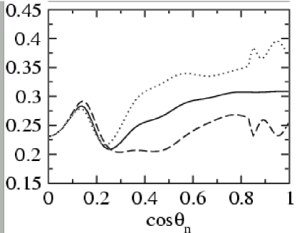
Figure 28: The nadir angle distribution of the charge asymmetry, $A_{\mu^{-}\mu^{+}}\equiv\frac{N(\mu^{-})-N(\mu^{+})}{N(\mu^{-})+N(\mu^{+})}$, measurable in magnetized calorimeters, of the multi-GeV $\mu^{-}-$ and $\mu^{+}-$ like events (or event rates), integrated over the neutrino (and muon) energy in the interval $E=(2.0-10.0)$ GeV, in the cases i) of two-neutrino $\nu_{\mu}\rightarrow\nu_{\tau}$ and $\bar{\nu}_{\mu}\rightarrow\bar{\nu}_{\tau}$ oscillations in vacuum and no $\nu_{e}$ and $\bar{\nu}_{e}$ oscillations, $A_{\mu^{-}\mu^{+}}^{2\nu}$ (solid lines), ii) three-neutrino oscillations of $\nu_{\mu}$, $\bar{\nu}_{\mu}$ $\nu_{e}$ and $\bar{\nu}_{e}$ in the Earth and neutrino mass spectrum with normal hierarchy $(A_{\mu^{-}\mu^{+}}^{3\nu})_{\rm NH}$ (dashed lines), or with inverted hierarchy, $(A_{\mu^{-}\mu^{+}}^{3\nu})_{\rm IH}$ (dotted lines). The results shown are for $|\mbox{$\Delta m^{2}_{23}$}|=3\times 10^{-3}~{}{\rm eV^{2}}$, $\sin^{2}\theta_{23}=~{}0.64$, and $\sin^{2}2\theta_{13}=0.05$. Figure taken from Ref. [113].

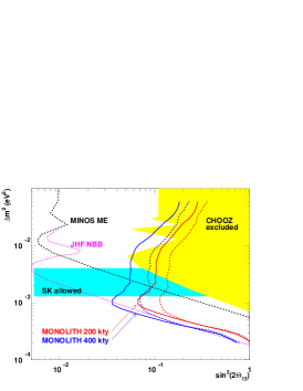
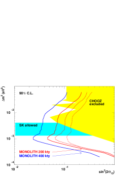
Figure 29: Left: Sensitivity regions at 90% C.L. in a MONOLITH-like iron calorimeter for 200 kton yrs (red lines) and 400 kton yrs (blue lines), for $\mbox{$\Delta m^{2}_{23}$}>0$ (solid lines) and $\mbox{$\Delta m^{2}_{23}$}<0$ (dashed lines). The regions excluded by CHOOZ and allowed by Super-Kamiokande (at the time this analysis was done), together with the expected sensitivity regions of MINOS (Medium Energy) and JHF (Low Energy) are also shown. Right: Sensitivity regions at 90% C.L. in a MONOLITH-like iron calorimeter for 200 kton yr (red solid line) and 400 kton yrs (blue line), for which the sign of $\Delta m^{2}_{23}$ can be determined, assuming that $\sin^{2}{2\theta_{13}}$ is known with a 30% accuracy. If no prior knowledge of $\sin^{2}{2\theta_{13}}$ is assumed, the regions over which the sign of $\Delta m^{2}_{23}$ can be determined, if it is positive (red dashed line) or negative (red dashed line), with an exposure of 200 kton-yr, are also depicted. Figures taken from Ref. [114].

Having the capability of discriminating the charge of the neutrino-induced muon, the observable (for magnetized calorimeters) which is the most sensitive to the value of $\sin^{2}{\theta_{13}}$ and the sign of $\Delta m^{2}_{23}$ is the charge asymmetry, $A_{\mu^{-}\mu^{+}}\equiv\frac{N(\mu^{-})-N(\mu^{+})}{N(\mu^{-})+N(\mu^{+})}$ for multi-GeV $\mu^{-}$ and $\mu^{+}$ event rates [113]. The qualitative behavior of this observable can be understood from the already explained matter effects for neutrinos crossing the Earth. In Fig. 28 we show an example of the nadir angle distribution of $A_{\mu^{-}\mu^{+}}$. From this figure we see that the distinction of the type of neutrino mass spectrum is in this case much more clear than in the case of water-Cerenkov detectors, each type having a different sign with respect to the case of 2-neutrino oscillations (see Ref. [113]).

An analysis of the sensitivity for an iron calorimeter like the proposed MONOLITH [114] is shown in Fig. 29; INO should be able to achieve similar results.

From these considerations and Figs. 26, 27,and  29, we learn that a magnetized detector is the preferred experiment to measure the sign of $\Delta m^{2}_{23}$ and the value of $\sin^{2}{2\theta_{13}}$ with atmospheric neutrinos.

4.3 Non-Oscillation Atmospheric Neutrino Studies

Aside from the dramatic physics discussed in previous sections, there are many related topics and many intimately intertwined areas of physics which need to be carried out to facilitate maximum exploitation of the solar and atmospheric neutrino research program. Here we briefly review some of the other physics topics which have been neglected up to this point. We remind the reader of the fantastic physics of supernova neutrinos studies, which lies in energy between solar and atmospheric studies and so is related in technology and backgrounds in physical detectors. We give an overview of the thorny issue of precision atmospheric neutrino calculations, which constrain our ability to use the atmospheric neutrino beam. We mention the necessity of updated accelerator measurements of hadronic and neutrino interactions as input to all this work, and finally we point out the necessity of ongoing support for the computer simulation tools which are mainstays of all these works.

4.3.1 Other Fundamental Physics

As discussed in Section 2, atmospheric neutrino detectors were designed originally to do other physics. The generality of the detector technology has allowed searches for a variety of particles such as magnetic monopoles, quark nuggets, Q-balls, WIMPs, free quarks, mirror particles, etc. In addition, we have studied the cosmic radiation in terms of content, spectrum, particle clustering in space and time, astronomical uniformity, temporal variation (correlation with solar cycles, etc.), sensitivity to atmospheric conditions (season, temperature) and correlations with events such as gamma ray bursts, solar outbreaks and bursting activity from distant quasars.

4.3.2 Supernova Neutrino Studies

As we mentioned in Section 3.6 for the planned solar neutrino experiments., many of the future atmospheric experiments can serve as detectors of neutrinos from supernovae.

The rate of galactic SN Types Ib/c and II (namely gravitational collapse) events in our galaxy is observationally only once per 250 years from historical records. Of course only a small fraction of the galaxy is visible by eye, perhaps 1/6. The rate from external galaxies (averaging over types) is about 1/60 years. We have had almost totally continuous neutrino monitoring now for about 20 years, but waiting for the next galactic SN requires patience. A detector like Super-Kamiokande can see of order 100k events in 10 s for a Type II supernova at the galactic center. Future, large-scale atmospheric experiments may be able to see 50 times more, hopefully allowing us to better understand the still ill-understood physics of stellar collapse.

In addition to seeing a burst of neutrinos from a supernova collapse in ‘real-time’, it may be possible to observe isolated neutrinos arriving from distant and dim SN, the so-called “Supernova relic neutrinos”. Those arriving from great distances (eg. z$>$1) will have significantly down-shifted spectra, encroaching upon the solar neutrino energy regime. Detection of such neutrinos could provide much interesting information on stellar origins and evolution. Antineutrino detectors offer the least background, until one gets down to below about 8 MeV and starts picking up background from terrestrial reactors. SuperK results come within about a factor of three of the most optimistic and credible models, and are limited by cosmic ray neutrino induced backgrounds. A large-scale water Cerenkov detector could see these, if it is located deep enough.

We suggest that the recommendation be that all detectors with SN detection capability should be encouraged, and that they should be encouraged to cooperate on a world wide basis to enable wide and prompt notification of the next supernova. A megaton detector with adequate energy sensitivity (for single neutrons) could provide coverage of the Milky Way.

4.3.3 Atmospheric Neutrino Flux

“Atmospheric neutrinos” arise from interactions of the incoming primary cosmic rays with the Earth’s atmosphere, which being not too dense permits many secondaries to decay, resulting in substantial neutrino fluxes. In fact the dominant neutrino flux on (and below) the earth’s surface between a few tens of MeV and perhaps 10 PeV arises from this halo of cosmic ray interactions typically 20km high in the atmosphere. In the first few GeV energy range, the ratios of neutrino types are well determined by the decay kinematics of pions and muons, of both signs. The ratio of $\pi^{+}$ to $\pi^{-}$ is about 5:4. Hence at such lower energies we have flux ratios known a priori to around 5%.

Calculations of atmospheric neutrino fluxes are generally carried out starting from the flux of primary cosmic rays, including non-trivial amounts of nuclei heavier than hydrogen, hitting air nuclei. Secondary particles may interact and cascade in the atmosphere, particularly at higher energies. Aside from knowing the incoming primary cosmic ray spectrum and compositions, one needs to know nucleus-nucleus cross-sections and partial cross-sections for all secondaries. Much of this is not well known. The most egregious deficiency is perhaps in the knowledge of the pion to kaon ratio in the forward direction. As one goes to higher energies the flux is dominated at first by pion decays, but beyond around 100 GeV by kaon decays.

Further complications in the atmospheric neutrino flux calculations are the earth’s magnetic field, which cuts off the incoming primary cosmic rays (up to a few GeV) depending upon magnetic latitude and which bends the secondary tracks of particles so that a straight line approximation is not adequate below a few GeV. Moreover when one is attempting to do better than tens of percent in these calculations, one needs to use a realistic atmosphere model, and perhaps even include seasonal effects (a warmer atmosphere is less dense and makes more neutrinos). There are also effects due to the state of solar activity, which are at present only crudely modeled.

The atmospheric neutrino flux even today remains frustratingly imprecise in absolute magnitude. The most recent calculations claim the accuracy has improved from around 25% to $<$10% below 10 GeV. Above a TeV it is perhaps uncertain to a factor of two! Even in the latest reduction of data from SuperK I (2004), the absolute normalization of the neutrino flux is allowed to float and they find it to be off (including oscillations) by 14.4% (more events seen than expected). Now one may be tempted to ignore such nuisances, but this lack of knowledge has effects on oscillations studies and every other physics analysis for which atmospheric neutrinos pose a background (eg. proton decay searches and searches for extraterrestrial neutrinos).

It is worth remarking that while variations in the atmospheric flux model have not changed the conclusions at all about muon neutrino oscillations taking place and being nearly maximal, the flux model can indeed move the derived $\Delta m^{2}$ around on the order of a factor of two. There has seemed to be a discrepancy between earlier and smaller experiments which inferred larger $\Delta m^{2}$ values based upon $\mu/e$ ratios, and the results of SuperK, which is pulled to lower values by shape (energy and angle) fits. Thus the influence of atmospheric neutrino flux calculations is significant when we start moving to the era of precise oscillation parameter measurements. Atmospheric neutrino flux measurements are also the limiting factor in searches for sub-dominant processes, and any new physics which might be showing up at second order.

The limited precision of the atmospheric flux calculations means that we remain unable to fully exploit the great dynamic range of the atmospheric natural beam. Our recommendation is that strong support be given to efforts to update hadronic interaction measurements (for which there is also need by those making neutrino beams) at accelerators (HARP, MIPP, NA-49), for better cosmic ray studies into the TeV regime, and for further improvements in flux modeling.

4.3.4 Neutrino Cross-sections

As stated above, improved hadronic cross-sections are needed for atmospheric (and accelerator) neutrino flux calculations. Interaction cross-section improvements are needed on the other end as well, in measurements of the neutrino partial cross sections. A key problem for atmospheric neutrino studies is predictions of interactions in the energy range of a few GeV. This is just the region where the transition from quasi-elastic to deep inelastic takes place, and where the theory is murky. Particularly central is the production of single $\pi^{o}$’s. This is because asymmetric $\pi^{o}$ decay mimics a single (CC) electron (positron), which is background for searches for muon to electron neutrino oscillations. Some work on this is underway or planned at the various long baseline experiments (eg. K2K, MINERVA, T2K).

4.4 Future Atmospheric Experiments

In this section we will briefly outline the future of existing and proposed experiments which may have the potential to carry out the atmospheric neutrino measurements discussed above.

4.4.1 Future of Super-K

Super-K’s current configuration is Super-K II with 47% of inner detector photomultiplier tubes; in this configuration atmospheric neutrino data quality is scarcely diminished from that of Super-K I[115]. Super-K will be replenished to its full complement of tubes during 2005/06, and Super-K III is expected to collect high quality atmospheric neutrino data for many years beyond that. The plots in section 4.2 give a sense of Super-K’s long term reach for $\theta_{13}$ and the sign of $\Delta m^{2}_{23}$, via atmospheric neutrinos.

4.4.2 SNO

Although SNO is a relatively small detector, it has two advantages as an atmospheric neutrino detector. The first is its depth and overburden: at over 6000 m.w.e, it is the deepest operating atmospheric neutrino detector. This depth, and the flat overburden, mean that SNO can measure the atmospheric neutrino flux using throughgoing muons even above the detector horizon (up to $\cos\eta=0.4$) without any contamination from cosmic ray muons. These data above the horizon are important, because they will tell us the unoscillated flux of neutrinos and therefore reduce the reliance on atmospheric neutrino flux models. In addition, the charged current interactions of antineutrinos within SNO should produce additional neutrons compared to neutrinos, and it may be possible to make a crude measurement of the relative rates ot these. SNO will continue running until the end of 2006, at which point it is likely to have over 1000 live-days of data.

4.5 Next Generation Water Cherenkov Detectors

Large next generation underground water Chrenkov detectors are proposed in US (UNO [116] [33]), in Japan (Hyper-Kamiokande [72]) and in Europe. These large megaton class detectors are proposed as multi-purpose detectors that probe physics beyond the sensitivities of the highly successful Super-Kamiokande detector utilizing a well- tested technology. The physics goals of these detectors include: nucleon decay searches, observation of neutrinos from supernova explosions, observation of supernova relic neutrinos, and precision measurements of neutrino oscillation parameters using atmospheric, solar and accelerator produced neutrinos.

The UNO detector is current proposed to be built in the Henderson mine located at Empire, Colorado. The optimal depth of the detector is considered to be about  4,000 mwe. The Hyper-Kamiokande detector is proposed to be build in the Tochibora mine, about 8 km away from the Kamioka mine in the west coast of the main island, Japan. The proposed detector site has a depth of 1400   1900 mwe. In Europe, an UNO-like detector is poposed to be built in the Frejus tunnel, which is located about 130 km from CERN. The detector can be located as deep as  4800 mwe.

Because of their sheer size that provides high statistics data and larger energy containment than Super-K, these detectors have capabilities to observe multiple oscillation minima and possibly determine mass hierarchy as described in the previous sections (see Sections 4.1.2 and 4.2) and to observe $\nu_{\tau}$ appearance in the atmospheric neutrinos. For the scale of detector discussed here, we would expect about 1 tau event per kton-year exposure, yielding about 400 tau events in one year.

4.5.1 MINOS

Among the operating detectors, MINOS is an iron magnetized calorimeter and thus, has muon charge identification capabilities for multi-GeV muons [92]. The MINOS experiment is currently collecting atmospheric neutrino data. The detector has relatively small mass, but after 5 years of data-taking it is expected to collect about 440 atmospheric $\nu_{\mu}$ and about 260 atmospheric $\bar{\nu}_{\mu}$ multi-GeV events (having the interaction vertex inside the detector). Reference [117] gives a summary of physics reach for MINOS from atmospheric neutrinos (in particular what can be learned from $\nu$ versus $\bar{\nu}$ tagging).

4.5.2 INO

There are also plans to build a 30-50 kton magnetized tracking iron calorimeter detector in India within the India-based Neutrino Observatory (INO) project [118]. The primary goal is to study the oscillations of atmospheric $\nu_{\mu}$ and $\bar{\nu}_{\mu}$. This detector is planned to have efficient muon charge identification, high muon energy resolution ($\sim 5\%$) and muon energy threshold of about 2 GeV. It will accumulate sufficiently high statistics of atmospheric $\nu_{\mu}$ and $\bar{\nu}_{\mu}$ induced events over several years, which would permit a search for the effects of the subdominant $\nu_{\mu}\rightarrow\nu_{e}$ ($\nu_{e}\rightarrow\nu_{\mu}$) and $\bar{\nu}_{\mu}\rightarrow\bar{\nu}_{e}$ ($\bar{\nu}_{e}\rightarrow\bar{\nu}_{\mu}$) transitions. The sensitivity to new physics should be comparable to that evaluated for a similar detector, MONOLITH (section 4.2 and Ref. [114]). A 30% effect—roughly the size we would expect for the best values of the mixing parameters—could be observed by INO with 5 years of running.

We have seen that both water Cerenkov and magnetized detectors have sensitivity to these effects; however a magnetized detector is a superior atmospheric neutrino experiment for measurement of the value of $\sin^{2}{2\theta_{13}}$ and the sign of $\Delta m^{2}_{23}$, due to ability to distinguish neutrinos and antineutrinos.

In conclusion, due to their large range of L/E and to the propagation through matter, $\theta_{13}-$driven resonant effects can show up in atmospheric neutrino experiments. Therefore, these experiments have direct access to a fundamental parameter in neutrino physics: the type of neutrino mass hierarchy.

5 Facilities

We note that for nearly all the experiments discussed here, underground facilities are a common element. We therefore recommend the development of underground space for use in both solar and atmospheric neutrino experiments.

References

- [1] R. Davis Jr., Solar neutrinos. II. Experimental, Phys. Rev. Lett. 12 (1964) 303.
- [2] T.J. Haines et al., Phys. Rev. Lett. 57, (1986).
- [3] D. Casper et al. Phys. Rev. Lett. 66, 2561 (1991)
- [4] K.S. Hirata et al., Physics Letters B205 pp. 416-420, 1988.
- [5] K.S. Hirata et al., Phys. Rev. Lett. 63, 16 (1989).
- [6] V.N. Gavrin, Proc. Int. Conf. on Topics in Astroparticle and Underground Physics, Seattle WA, Sept. 5 -9, 2003.
- [7] GALLEX collaboration, W. Hampel et al., GALLEX solar neutrino observations: results for GALLEX IV, Phys. Lett. B 447 (1999) 127.
- [8] S. Fukuda et al., Phys. Lett. B539, 179 (2002); Phys. Rev. Lett. 86, 5651 (2001).
- [9] SNO Collaboration: Q.R. Ahmad et al., Phys. Rev. Lett. 87, 071301 (2001)
- [10] E. Bellotti, Proc. Int. Conf. on Topics in Astroparticle and Underground Physics, Seattle WA, Sept. 5 -9, 2003.
- [11] SNO Collaboration: Q.R. Ahmad et al., Phys. Rev. Lett. 89, 011301 (2002)
- [12] SNO Collaboration: Q.R. Ahmad et al., Phys. Rev. Lett. 89, 011302 (2002).
- [13] SNO Collaboration: S. N. Ahmed et al. nucl-ex/0309004.
- [14] http://www.sns.ias.edu/ jnb/
- [15] M. B.. Smy et al., Phys. Rev. D69, 011104, (2004).
- [16] J.N. Bahcall, Phys. Rev. Lett. 12, pp. 300-302, 1964.
- [17] J.N. Bahcall and C. Peña-Garay, JHEP 0311:004, 2003,(hep-ph/0305159v3).
- [18] B.T. Cleveland et al., Astrophys. J. 496, 505 (1998).
- [19] V. Gavrin, Results from the Russian American gallium experiment (SAGE), talk at VIIIth International Conference on Topics in Astroparticle and Underground Physics (TAUP03), Seattle, Sept. 5–9, 2003; SAGE collaboration, J.N. Abdurashitov et al., J. Exp. Theor. Phys. 95 (2002) 181 [astro-ph/0204245].
- [20] KamLAND Collaboration: K. Eguchi et al. Phys. Rev. Lett 90 021802 (2003) [hep-ex/0212021].
- [21] J. N. Bahcall ”Solar Models: An Historical Overview”, Nucl. Phys. B (Proc. Suppl.), 118, 77 (2003).
- [22] M. Gasperini, Phys. Rev. D 38 (1988) 2635; Phys. Rev. D 39, 3606 (1989);
- [23] V. De Sabbata and M. Gasperini, Nuovo Cimento A 65, 479 (1981).
- [24] S. Coleman and S.L. Glashow, Phys. Lett. B 405, 249 (1997); S.L. Glashow, A. Halprin, P.I. Krastev, C.N. Leung, and J. Pantaleone, Phys. Rev. D 56, 2433 (1997).
- [25] L. Wolfenstein, Phys. Rev. D17, 236 (1978)
- [26] D. Colladay and V.A. Kostelecky, Phys. Rev. D55, 6760 (1997); S. Coleman and S.L. Glashow, Phys. Rev. D 59, 116008 (1999).
- [27] A. M. Gago, M. M. Guzzo, P. C. de Holanda, H. Nunokawa, O. L. G. Peres, V. Pleitez and R. Zukanovich Funchal, Phys. Rev. D 65, 073012 (2002)
- [28] V. Barger, D. Marfatia, K. Whisnant, B. Wood, hep-ph/0204253.
- [29] David B. Kaplan, Ann E. Nelson, and Neal Weiner, hep-ph/0401099.
- [30] J. N. Bahcall and C. Pena-Garay, JHEP 0311, 004 (2003)
- [31] M. M. Guzzo, P. C. de Holanda and O. L. G. Peres, hep-ph/0403134.
- [32] P.C. de Holanda and A.Yu. Smirnov, Astropart. Phys.21, 287-301, (2004).
- [33] Physics Potential and Feasibility of UNO (UNO Whitepaper), ed. D. Casper, C.K. Jung, C. McGrew, and C. Yanagisawa, June 2001, SBHEP01-3.
- [34] M.V. Diwan et al, hep-ex/0306053, June 2003.
- [35] J.N. Bahcall and C. Peña-Garay, New Journal of Physics 6 (2004), 63.
- [36] KamLAND Collaboration: T. Araki et al. [hep-ex/0406035], 2004.
- [37] Y. Fukuda et al. [Super-Kamiokande Collaboration], Phys. Rev. Lett. 81, 1562 (1998).
- [38] T. Toshito, for the Super-Kamiokande Collaboration, hep-ex/0105023
- [39] MACRO Collaboration: M. Ambrosio et al, Phys. Lett. B 434, 451 (1998).
- [40] Soudan-2 Collaboration: W.W.M. Allison et al, Phys. Lett. B 449, 137 (1999).
- [41] C. Saji, Proc. Conf. NOON04, http://www-sk.icrr.u-tokyo.ac.jp/noon2004/.
- [42] O. L. Peres and A. Y. Smirnov, Phys. Lett. B 456, 204 (1999); O. L. Peres and A. Y. Smirnov, Nucl. Phys. Proc. Suppl. 110 (2002) 355.
- [43] M. C. Gonzalez-Garcia and M. Maltoni, Eur. Phys. J. C 26, 417 (2003)
- [44] P. Huber, M. Lindner, M. Rolinec, T. Schwetz and W. Winter, arXiv:hep-ph/0403068.
- [45] L. Wolfenstein, Neutrino oscillations in matter, Phys. Rev. D 17 (1978) 2369; S.P. Mikheyev and A.Y. Smirnov, Resonance enhancement of oscillations in matter and solar neutrino spectroscopy, Sov. Jour. Nucl. Phys. 42 (1985) 913.
- [46] H.A. Bethe, Possible explanation of the solar-neutrino puzzle, Phys. Rev. Lett. 56 (1986) 1305.
- [47] S.P. Mikheev and A.Y. Smirnov, Neutrino oscillations in matter with varying density, Proc. of the 6th Moriond Workshop on Massive Neutrinos in Astrophysics and Particle Physics, eds. O. Fackler and J. Tran Thanh Van (Editions Frontières 1986), p. 355.
- [48] G. L. Fogli, E. Lisi, A. Marrone and G. Scioscia, Phys. Rev. D 60, 053006 (1999)
- [49] A. Messiah, Treatment of electron-neutrino oscillations in solar matter: the MSW Effect, Proc. of the 6th Moriond Workshop on Massive Neutrinos in Astrophysics and Particle Physics, eds. O. Fackler and J. Tran Thanh Van (Editions Frontières 1986), p. 373.
- [50] J.N. Bahcall, Neutrino Astrophysics, Cambridge University Press, Cambridge, 1989.
- [51] M.C. Gonzalez-Garcia and Y. Nir, Neutrino masses and mixing: evidence and implications, Rev. Mod. Phys. 75 (2003) 345 [hep-ph/0202058].
- [52] M.Maltoni, T. Schwetz, M.A. Tórtola, and J.W.F. Valle, hep-ph/0309130v2.
- [53] M.C.Gonzalez-Garcia, M. Maltoni hep-ph/0404085.
- [54] M.C. Gonzalez-Garcia and C. Peña-Garay, hep-ph/0111432v2.
- [55] K2K Collaboration: M.H. Ahn et al. Phys. Rev. Lett. 90, 041801 (2003); hep-ex/0212007.
- [56] G.L. Fogli, E. Lisi, and A. Marrone, Phys. Rev. D64, 093005 (2001); hep-ph/0105139
- [57] G.L. Fogli, E. Lisi, D. Montanino, and A. Palazzo, Phys. Rev. D62, 013002 (2000);hep-ph/9912231
- [58] K.M. Heeger and R.G.H. Robertson, Phys. Rev. Lett. 77, 3720 (1996).
- [59] , R.G.H. Robertson, “Solar Neutrinos and ”, in preparation, 2004.
- [60] J.N. Bahcall, M.C. Gonzalez-Garcia, and C. Peña-Garay, hep-ph/0406294v1 (2004).
- [61] M. Spiro and D. Vignaud, Phys. Lett. B 242, 279 (1990).
- [62] J.N. Bahcall, Phys. Rev. C 65, 025801 (2003).
- [63] J.N. Bahcall and M.H. Pinsonneault, Revs. Mod. Phys. 67, 781(1995).
- [64] J.N. Bahcall, Phys. Rev. 135, B137 (1964); ibid.Nucl. Phys. B (Proc. Suppl.) 38, 98 (1995).
- [65] J.N. Bahcall and R.K. Ulrich, Revs. Mod. Phys. 60, 297(1988).
- [66] J.N. Bahcall, Revs. Mod. Phys. 50, 881 (1978).
- [67] J.N. Bahcall, E. Lisi, D.E. Alburger, L. deBraeckeleer, S.J.Freedman, and J. Napolitano, Phys. Rev. C 54, 411 (1996).
- [68] W. Trinder et al., Phys. Lett. B349, 267 (1995).
- [69] W. Hampel and R. Schlotz, Proc. Intern. Conf. Atomic Massesand Fundamental Constants 7, Darmstadt-Seeheim (TH Darmstadt Lehrdruckerei,1984), p. 89.
- [70] N. Hata and W.C. Haxton, Phys. Lett. B353, 422 (1995).
- [71] J.N. Bahcall and M. H. Pinsonneault; Phys. Rev. Lett. 92(2004)121301.
- [72] Y. Itow et al, hep-ex/0106019v1, 2001.
- [73] The Borexino Collaboration, G. Alimonti et al., “Science and technology of Borexino: a real-time detector for low energy solar neutrinos”, Astrop. Phys., 16(3), 205 (2002).
- [74] L. Cadonati, “The Borexino Solar Neutrino Experiment and its Scintillator Containment Vessel”, Ph.D. Thesis, Princeton University, Jan. 2001.
- [75] A. Pocar, “Low Background Techniques and Experimental Challenges for Borexino and its Nylon Vessels”, Ph.D. Thesis, Princeton University, Nov. 2003.
- [76] G. Alimonti et al., “Ultra-low background measurements in a large volume underground detector”, Astrop. Phys., 8(3), 141 (1998).
- [77] C. Allende Prieto, D.L. Lambert, and M. Asplund; ApJ 556(2001)L63. C. Allende Prieto, D.L. Lambert, and M. Asplund; ApJ 573(2002)L137. M. Asplund, N. Grevesse, A.J. Sauval, C. Allende Prieto, and D. Kiselman, A&A, in press, astro-ph/0312290;
- [78] J.N. Bahcall, and A.M. Serenelli; astro-ph/0403604.
- [79] G. Fiorentini and B. Ricci; astro-ph/0310753.
- [80] S. Couvidat,S. Turck-Chie‘ze, and A. G. Kosovichev; bitemAdel E.G. Adelberger et al.; Rev. of Modern Phys. 70(1998)1265.
- [81] E.G. Adelberger et al.; Rev. of Modern Phys. 70(1998)1265.
- [82] M. Gai; nucl-ex/0312003.
- [83] A.R. Junghans et al.; Phys. Rev. Lett 88(2002)041101, ibid Phys. Rev. C68(2003)065803.
- [84] L.T. Baby et al., Phys. Rev. Lett. 90(2003)022501, ibid Phys. Rev. C67(2003)065805.
- [85] N. Iwasa et al.; Phys. Rev. Lett. 83(1999)2910.
- [86] F. Schumann et al.; Phys. Rev. Lett. 90(2003)232501.
- [87] R.G.H. Robertson et al.; Phys. Rev. C27(1983)27.
- [88] Hugh Gallagher, Neutrino 2004 talk
- [89] T. Nakaya, Neutrino 2004 talk
- [90] [Super-Kamiokande Collaboration], hep-ex/0404034
- [91] M.C. González-García, Talk given at the Int. Workshop on Neutrino Oscillations and their Origin (NOON2004), February 11 - 15, 2004, Tokyo, Japan.
- [92] D. Michael (MINOS Collaboration), Talk at the Int. Conf. on Neutrino Physics and Astrophysics “Neutrino’02”, May 25 - 30, 2002, Munich, Germany.
- [93] M. Komatsu, P. Migliozzi and F. Terranova, J. .Phys. G 29 (2003) 443.
- [94] M. Spiro, Summary talk at the Int. Conf. on Neutrino Physics and Astrophysics “Neutrino’02”, May 25 - 30, 2002, Munich, Germany.
- [95] A. De Rújula, M. B. Gavela and P. Hernández, Nucl. Phys. B 547, 21 (1999); V. Barger et al., Phys. Rev. D 62, 013004 (2000).
- [96] M. Freund et al., Nucl. Phys. B 578 (2000) 27.
- [97] V. Barger, D. Marfatia and K. Whisnant, Phys. Lett. B 560 (2003) 75; P. Huber, M. Lindner and W. Winter, Nucl. Phys. B 654 (2003) 3
- [98] S. M. Bilenky, S. Pascoli and S. T. Petcov, Phys. Rev. D 64 (2001) 053010; S. M. Bilenky et al., Phys. Lett. B 465 (1999) 193.
- [99] S. Pascoli and S. T. Petcov, Phys. Lett. B 544 (2002) 239, and Phys. Lett. B 580 (2004) 280; S. Pascoli, S. T. Petcov and W. Rodejohann, Phys. Lett. B 558 (2003) 141.
- [100] T. Kajita, Talk given at the Int. Workshop on Neutrino Oscillations and their Origin (NOON2004), February 11 - 15, 2004, Tokyo, Japan.
- [101] A. Friedland, C. Lunardini, and Michele Maltoni, Phys. Rev. D 70, p. 111301, (2004).
- [102] S. T. Petcov, Phys. Lett. B 434 (1998) 321, (E) ibid. B 444 (1998) 584.
- [103] E. K. Akhmedov et al., Nucl. Phys. B 542, 3 (1999).
- [104] J. Bernabéu, S. Palomares-Ruiz, A. Pérez and S. T. Petcov, Phys. Lett. B 531, 90 (2002)
- [105] S. T. Petcov, Phys. Lett. B 214, 259 (1988).
- [106] S. T. Petcov, Nucl. Phys. B (Proc. Suppl.) 77 (1999) 93, hep-ph/9809587, hep-ph/9811205 and hep-ph/9907216; M. V. Chizhov, M. Maris and S. T. Petcov, hep-ph/9810501.
- [107] M. V. Chizhov and S. T. Petcov, Phys. Rev. D 63 (2001) 073003.
- [108] M. C. Bañuls, G. Barenboim and J. Bernabéu, Phys. Lett. B 513, 391 (2001); J. Bernabéu and S. Palomares-Ruiz, hep-ph/0112002, and Nucl. Phys. Proc. Suppl. 110, 339 (2002), hep-ph/0201090.
- [109] M. V. Chizhov and S.T. Petcov, Phys. Rev. Lett. 83 (1999) 1096.
- [110] P. Langacker et al., Nucl. Phys. B282 (1987) 589.
- [111] J. Bernabéu, S. Palomares Ruiz and S. T. Petcov, Nucl. Phys. B 669, 255 (2003); S. Palomares-Ruiz and J. Bernabéu, hep-ph/0312038.
- [112] S. T. Petcov and S. Palomares-Ruiz, hep-ph/0406106.
- [113] S. Palomares-Ruiz and S. T. Petcov, hep-ph/0406096.
- [114] T. Tabarelli de Fatis, Eur. Phys. J. C 24 (2002) 43.
- [115] E. Kearns, Neutrino 2004 talk
- [116] C.K. Jung, Feasibility of a Next Generation Underground Water Cherenkov Detector: UNO, (hep-ex/0005046); Next Generation Nucleon Decay and Neutrino Detector, AIP Conf. Proc. 533, edited by M.V. Diwan and C.K. Jung (2000).
-
[117]
MINOS collaboration document,
http://www-numi.fnal.gov/numinotes/public/ps/numi1037/numi1037.ps.gz -
[118]
See http://www.imsc.res.in/ino
and working reports and talks therein.