EUROPEAN ORGANIZATION FOR NUCLEAR RESEARCH

CERN-PH-EP/2004-069

LEPEWWG/2004-01

ALEPH 2004-010 PHYSIC 2004-002

DELPHI 2004-049 PHYS 943

L3 Note 2828

OPAL PR 406

hep-ex/0412015

6 December 2004

A Combination of Preliminary
Electroweak Measurements and
Constraints on the Standard Model

The LEP Collaborations ALEPH, DELPHI, L3, OPAL,
the LEP Electroweak Working Group,
the SLD Electroweak and Heavy Flavour Groups

Prepared from Contributions of the LEP and SLD Experiments
to the 2004 Summer Conferences.

This note presents a combination of published and preliminary electroweak results from the four LEP collaborations and the SLD collaboration which were prepared for the 2004 summer conferences. Averages from $\mathrm{Z}$ resonance results are derived for hadronic and leptonic cross sections, the leptonic forward-backward asymmetries, the $\tau$ polarisation asymmetries, the $\mathrm{b\overline{b}}$ and $\mathrm{c\overline{c}}$ partial widths and forward-backward asymmetries and the $\mathrm{q\overline{q}}$ charge asymmetry. Above the $\mathrm{Z}$ resonance, averages are derived for di-fermion cross sections and forward-backward asymmetries, photon-pair, W-pair, Z-pair, single-W and single-Z cross sections, electroweak gauge boson couplings, W mass and width and W decay branching ratios. Also, an investigation of the interference of photon and Z-boson exchange is presented, and colour reconnection and Bose-Einstein correlation analyses in W-pair production are combined. The main changes with respect to the experimental results presented in summer 2003 are updates to the W branching fractions and four-fermion cross sections measured at LEP-2, and the SLD/LEP heavy-flavour results measured at the Z pole.

The results are compared with precise electroweak measurements from other experiments, notably the final result on the electroweak mixing angle determined in neutrino-nucleon scattering by the NuTeV collaboration, the latest result in atomic parity violation in Caesium, and the measurement of the electroweak mixing angle in Moller scattering. The parameters of the Standard Model are evaluated, first using the combined LEP electroweak measurements, and then using the full set of high-$Q^{2}$ electroweak results.

Chapter 1 Introduction

This paper presents an update of combined results on electroweak parameters by the four LEP experiments and SLD using published and preliminary measurements, superseding previous analyses[1]. Results derived from the $\mathrm{Z}$ resonance are based on data recorded until the end of 1995 for the LEP experiments and 1998 for SLD. Since 1996 LEP has run at energies above the W-pair production threshold. In 2000, the final year of data taking at LEP, the total delivered luminosity was as high as in 1999; the maximum centre-of-mass energy attained was close to 209 GeV although most of the data taken in 2000 was collected at 205 and 207 GeV. By the end of LEP-II operation, a total integrated luminosity of approximately 700$\mathrm{pb^{-1}}$ per experiment has been recorded above the Z resonance.

The LEP-I (1990-1995) $\mathrm{Z}$-pole measurements consist of the hadronic and leptonic cross sections, the leptonic forward-backward asymmetries, the $\tau$ polarisation asymmetries, the $\mathrm{b\overline{b}}$ and $\mathrm{c\overline{c}}$ partial widths and forward-backward asymmetries and the $\mathrm{q\overline{q}}$ charge asymmetry. The measurements of the left-right cross section asymmetry, the $\mathrm{b\overline{b}}$ and $\mathrm{c\overline{c}}$ partial widths and left-right-forward-backward asymmetries for b and c quarks from SLD are treated consistently with the LEP data. Many technical aspects of their combination are described in References 2, 3 and references therein.

The LEP-II (1996-2000) measurements are di-fermion cross sections and forward-backward asymmetries; di-photon production, W-pair, Z-pair, single-W and single-Z production cross sections, and electroweak gauge boson self couplings. W boson properties, like mass, width and decay branching ratios are also measured. New studies on photon/Z interference in fermion-pair production as well as on colour reconnection and Bose-Einstein correlations in W-pair production are presented.

Several measurements included in the combinations are still preliminary.

This note is organised as follows:

Chapter 2

$\mathrm{Z}$ line shape and leptonic forward-backward asymmetries;

Chapter 3

$\tau$ polarisation;

Chapter 4

Measurement of polarised asymmetries at SLD;

Chapter 5

Heavy flavour analyses;

Chapter 6

Inclusive hadronic charge asymmetry;

Chapter 7

Photon-pair production at energies above the Z;

Chapter 8

Fermion-pair production at energies above the Z;

Chapter 9

Photon/Z-boson interference;

Chapter 10

W and four-fermion production;

Chapter 11

Electroweak gauge boson self couplings;

Chapter 12

Colour reconnection in W-pair events;

Chapter 13

Bose-Einstein correlations in W-pair events;

Chapter 14

W-boson mass and width;

Chapter 15

Interpretation of the Z-pole results in terms of effective couplings of the neutral weak current;

Chapter 16

Interpretation of all results, also including results from neutrino interaction and atomic parity violation experiments as well as from CDF and DØ  in terms of constraints on the Standard Model

Chapter 17

Conclusions including prospects for the future.

To allow a quick assessment, a box highlighting the updates is given at the beginning of each chapter.

Chapter 2 $\mathrm{Z}$ Lineshape and Lepton Forward-Backward Asymmetries

Updates with respect to summer 2003:
Unchanged w.r.t. summer 2000: All experiments have published final results which enter in the combination. The final combination procedure is used, the obtained averages are final.

The results presented here are based on the full LEP-I data set. This includes the data taken during the energy scans in 1990 and 1991 in the range $|\sqrt{s}-m_{\mathrm{Z}}|<3$ GeV, the data collected at the $\mathrm{Z}$ peak in 1992 and 1994 and the precise energy scans in 1993 and 1995 ($|\sqrt{s}-m_{\mathrm{Z}}|<1.8$ GeV). The total event statistics are given in Table 2.1. Details of the individual analyses can be found in References 4, 5, 6, 7.

$\mathrm{q\overline{q}}$ year A D L O all ’90/91 433 357 416 454 1660 ’92 633 697 678 733 2741 ’93 630 682 646 649 2607 ’94 1640 1310 1359 1601 5910 ’95 735 659 526 659 2579 total 4071 3705 3625 4096 15497

$\ell^{+}\ell^{-}$ year A D L O all ’90/91 53 36 39 58 186 ’92 77 70 59 88 294 ’93 78 75 64 79 296 ’94 202 137 127 191 657 ’95 90 66 54 81 291 total 500 384 343 497 1724

Table 2.1: The $\mathrm{q\overline{q}}$ and $\ell^{+}\ell^{-}$ event statistics, in units of $10^{3}$, used for the analysis of the $\mathrm{Z}$ line shape and lepton forward-backward asymmetries by the experiments ALEPH (A), DELPHI (D), L3 (L) and OPAL (O).

For the averaging of results the LEP experiments provide a standard set of 9 parameters describing the information contained in hadronic and leptonic cross sections and leptonic forward-backward asymmetries. These parameters are convenient for fitting and averaging since they have small correlations. They are:

• The mass $m_{\mathrm{Z}}$ and total width $\Gamma_{\mathrm{Z}}$ of the Z boson, where the definition is based on the Breit-Wigner denominator $(s-m_{\mathrm{Z}}^{2}+is\Gamma_{\mathrm{Z}}/m_{\mathrm{Z}})$ with $s$-dependent width [8].

• The hadronic pole cross section of Z exchange:

  $$\sigma_{\mathrm{h}}^{0}\equiv{12\pi\over m_{\mathrm{Z}}^{2}}{\Gamma_{\mathrm{ee}}\Gamma_{\mathrm{had}}\over\Gamma_{\mathrm{Z}}^{2}}\,.$$ (2.1)

  Here $\Gamma_{\mathrm{ee}}$ and $\Gamma_{\mathrm{had}}$ are the partial widths of the $\mathrm{Z}$ for decays into electrons and hadrons.

• The ratios:

  $$R^{0}_{\mathrm{e}}\equiv\Gamma_{\mathrm{had}}/\Gamma_{\mathrm{ee}},\;\;R^{0}_{\mu}\equiv\Gamma_{\mathrm{had}}/\Gamma_{\mu\mu}\;\mbox{and}\;R^{0}_{\tau}\equiv\Gamma_{\mathrm{had}}/\Gamma_{\tau\tau}.$$ (2.2)

  Here $\Gamma_{\mu\mu}$ and $\Gamma_{\tau\tau}$ are the partial widths of the $\mathrm{Z}$ for the decays $\mathrm{Z}\rightarrow\mu^{+}\mu^{-}$ and $\mathrm{Z}\rightarrow\tau^{+}\tau^{-}$. Due to the mass of the $\tau$ lepton, a difference of 0.2% is expected between the values for $R^{0}_{\mathrm{e}}$ and $R^{0}_{\mu}$, and the value for $R^{0}_{\tau}$, even under the assumption of lepton universality [9].

• The pole asymmetries, $A^{0,\,{\mathrm{e}}}_{\mathrm{FB}}$, $A^{0,\,\mu}_{\mathrm{FB}}$ and $A^{0,\,\tau}_{\mathrm{FB}}$, for the processes $\mathrm{e}^{+}\mathrm{e}^{-}\rightarrow\mathrm{e}^{+}\mathrm{e}^{-}$, $\mathrm{e}^{+}\mathrm{e}^{-}\rightarrow\mu^{+}\mu^{-}$ and $\mathrm{e}^{+}\mathrm{e}^{-}\rightarrow\tau^{+}\tau^{-}$. In terms of the real parts of the effective vector and axial-vector neutral current couplings of fermions, $g_{\mathrm{Vf}}$ and $g_{\mathrm{Af}}$, the pole asymmetries are expressed as

  $$A^{0,\,{\mathrm{f}}}_{\mathrm{FB}}\equiv{3\over 4}{\cal A}_{\mathrm{e}}{\cal A}_{\mathrm{f}}$$ (2.3)

  with

  $${\cal A}_{\mathrm{f}}\equiv\frac{2g_{\mathrm{Vf}}g_{\mathrm{Af}}}{g_{\mathrm{Vf}}^{2}+g_{\mathrm{Af}}^{2}}\ =2\frac{g_{\mathrm{Vf}}/g_{\mathrm{Af}}}{1+(g_{\mathrm{Vf}}/g_{\mathrm{Af}})^{2}}\,.$$ (2.4)

The imaginary parts of the vector and axial-vector coupling constants as well as real and imaginary parts of the photon vacuum polarisation are taken into account explicitly in the fitting formulae and are fixed to their Standard Model values. The fitting procedure takes into account the effects of initial-state radiation [8] to ${\cal O}(\alpha^{3})$ [10, 11, 12], as well as the $t$-channel and the $s$-$t$ interference contributions in the case of $\mathrm{e}^{+}\mathrm{e}^{-}$ final states.

The set of 9 parameters does not describe hadron and lepton-pair production completely, because it does not include the interference of the $s$-channel $\mathrm{Z}$ exchange with the $s$-channel $\gamma$ exchange. For the results presented in this section and used in the rest of the note, the $\gamma$-exchange contributions and the hadronic $\gamma\mathrm{Z}$ interference terms are fixed to their Standard Model values. The leptonic $\gamma\mathrm{Z}$ interference terms are expressed in terms of the effective couplings.

		correlations
		$m_{\mathrm{Z}}$	$\Gamma_{\mathrm{Z}}$	$\sigma_{\mathrm{h}}^{0}$	$R^{0}_{\mathrm{e}}$	$R^{0}_{\mu}$	$R^{0}_{\tau}$	$A^{0,\,{\mathrm{e}}}_{\mathrm{FB}}$	$A^{0,\,\mu}_{\mathrm{FB}}$	$A^{0,\,\tau}_{\mathrm{FB}}$
$\phantom{00}\chi^{2}/N_{\rm df}\,=\,169/176$		ALEPH
$m_{\mathrm{Z}}$ [GeV]	91.1891 $\pm$ 0.0031	1.00
$\Gamma_{\mathrm{Z}}$ [GeV]	2.4959 $\pm$ 0.0043	.038	1.00
$\sigma_{\mathrm{h}}^{0}$ [nb]	41.558 $\pm$ 0.057	$-$.091	$-$.383	1.00
$R^{0}_{\mathrm{e}}$	20.690 $\pm$ 0.075	.102	.004	.134	1.00
$R^{0}_{\mu}$	20.801 $\pm$ 0.056	$-$.003	.012	.167	.083	1.00
$R^{0}_{\tau}$	20.708 $\pm$ 0.062	$-$.003	.004	.152	.067	.093	1.00
$A^{0,\,{\mathrm{e}}}_{\mathrm{FB}}$	0.0184 $\pm$ 0.0034	$-$.047	.000	$-$.003	$-$.388	.000	.000	1.00
$A^{0,\,\mu}_{\mathrm{FB}}$	0.0172 $\pm$ 0.0024	.072	.002	.002	.019	.013	.000	$-$.008	1.00
$A^{0,\,\tau}_{\mathrm{FB}}$	0.0170 $\pm$ 0.0028	.061	.002	.002	.017	.000	.011	$-$.007	.016	1.00
$\phantom{00}\chi^{2}/N_{\rm df}\,=\,177/168$		DELPHI
$m_{\mathrm{Z}}$ [GeV]	91.1864 $\pm$ 0.0028	1.00
$\Gamma_{\mathrm{Z}}$ [GeV]	2.4876 $\pm$ 0.0041	.047	1.00
$\sigma_{\mathrm{h}}^{0}$ [nb]	41.578 $\pm$ 0.069	$-$.070	$-$.270	1.00
$R^{0}_{\mathrm{e}}$	20.88 $\pm$ 0.12	.063	.000	.120	1.00
$R^{0}_{\mu}$	20.650 $\pm$ 0.076	$-$.003	$-$.007	.191	.054	1.00
$R^{0}_{\tau}$	20.84 $\pm$ 0.13	.001	$-$.001	.113	.033	.051	1.00
$A^{0,\,{\mathrm{e}}}_{\mathrm{FB}}$	0.0171 $\pm$ 0.0049	.057	.001	$-$.006	$-$.106	.000	$-$.001	1.00
$A^{0,\,\mu}_{\mathrm{FB}}$	0.0165 $\pm$ 0.0025	.064	.006	$-$.002	.025	.008	.000	$-$.016	1.00
$A^{0,\,\tau}_{\mathrm{FB}}$	0.0241 $\pm$ 0.0037	.043	.003	$-$.002	.015	.000	.012	$-$.015	.014	1.00
$\phantom{00}\chi^{2}/N_{\rm df}\,=\,158/166$		L3
$m_{\mathrm{Z}}$ [GeV]	91.1897 $\pm$ 0.0030	1.00
$\Gamma_{\mathrm{Z}}$ [GeV]	2.5025 $\pm$ 0.0041	.065	1.00
$\sigma_{\mathrm{h}}^{0}$ [nb]	41.535 $\pm$ 0.054	.009	$-$.343	1.00
$R^{0}_{\mathrm{e}}$	20.815 $\pm$ 0.089	.108	$-$.007	.075	1.00
$R^{0}_{\mu}$	20.861 $\pm$ 0.097	$-$.001	.002	.077	.030	1.00
$R^{0}_{\tau}$	20.79 $\phantom{0}\pm$ 0.13	.002	.005	.053	.024	.020	1.00
$A^{0,\,{\mathrm{e}}}_{\mathrm{FB}}$	0.0107 $\pm$ 0.0058	$-$.045	.055	$-$.006	$-$.146	$-$.001	$-$.003	1.00
$A^{0,\,\mu}_{\mathrm{FB}}$	0.0188 $\pm$ 0.0033	.052	.004	.005	.017	.005	.000	.011	1.00
$A^{0,\,\tau}_{\mathrm{FB}}$	0.0260 $\pm$ 0.0047	.034	.004	.003	.012	.000	.007	$-$.008	.006	1.00
$\phantom{00}\chi^{2}/N_{\rm df}\,=\,155/194$		OPAL
$m_{\mathrm{Z}}$ [GeV]	91.1858 $\pm$ 0.0030	1.00
$\Gamma_{\mathrm{Z}}$ [GeV]	2.4948 $\pm$ 0.0041	.049	1.00
$\sigma_{\mathrm{h}}^{0}$ [nb]	41.501 $\pm$ 0.055	.031	$-$.352	1.00
$R^{0}_{\mathrm{e}}$	20.901 $\pm$ 0.084	.108	.011	.155	1.00
$R^{0}_{\mu}$	20.811 $\pm$ 0.058	.001	.020	.222	.093	1.00
$R^{0}_{\tau}$	20.832 $\pm$ 0.091	.001	.013	.137	.039	.051	1.00
$A^{0,\,{\mathrm{e}}}_{\mathrm{FB}}$	0.0089 $\pm$ 0.0045	$-$.053	$-$.005	.011	$-$.222	$-$.001	.005	1.00
$A^{0,\,\mu}_{\mathrm{FB}}$	0.0159 $\pm$ 0.0023	.077	$-$.002	.011	.031	.018	.004	$-$.012	1.00
$A^{0,\,\tau}_{\mathrm{FB}}$	0.0145 $\pm$ 0.0030	.059	$-$.003	.003	.015	$-$.010	.007	$-$.010	.013	1.00

Table 2.2: Line Shape and asymmetry parameters from fits to the data of the four LEP experiments and their correlation coefficients.

The four sets of nine parameters provided by the LEP experiments are presented in Table 2.2. For performing the average over these four sets of nine parameters, the overall covariance matrix is constructed from the covariance matrices of the individual LEP experiments and taking into account common systematic errors [2]. The common systematic errors include theoretical errors as well as errors arising from the uncertainty in the LEP beam energy. The beam energy uncertainty contributes an uncertainty of $\pm 1.7\leavevmode\nobreak\ {\mathrm{Me\kern-1.00006ptV}}$ to $m_{\mathrm{Z}}$ and $\pm 1.2\leavevmode\nobreak\ {\mathrm{Me\kern-1.00006ptV}}$ to $\Gamma_{\mathrm{Z}}$. In addition, the uncertainty in the centre-of-mass energy spread of about $\pm 1\leavevmode\nobreak\ {\mathrm{Me\kern-1.00006ptV}}$ contributes $\pm 0.2\leavevmode\nobreak\ {\mathrm{Me\kern-1.00006ptV}}$ to $\Gamma_{\mathrm{Z}}$. The theoretical error on calculations of the small-angle Bhabha cross section is $\pm$0.054 %[13] for OPAL and $\pm$0.061 %[14] for all other experiments, and results in the largest common systematic uncertainty on $\sigma_{\mathrm{h}}^{0}$. QED radiation, dominated by photon radiation from the initial state electrons, contributes a common uncertainty of $\pm$0.02 % on $\sigma_{\mathrm{h}}^{0}$, of $\pm 0.3$ MeV on $m_{\mathrm{Z}}$ and of $\pm 0.2$ MeV on $\Gamma_{\mathrm{Z}}$. The contribution of $t$-channel diagrams and the $s$-$t$ interference in $\mathrm{Z}\rightarrow\mathrm{e}^{+}\mathrm{e}^{-}$ leads to an additional theoretical uncertainty estimated to be $\pm 0.024$ on $R^{0}_{\mathrm{e}}$ and $\pm 0.0014$ on $A^{0,\,{\mathrm{e}}}_{\mathrm{FB}}$, which are fully anti–correlated. Uncertainties from the model-independent parameterisation of the energy dependence of the cross section are almost negligible, if the definitions of Reference [15] are applied. Through unavoidable remaining Standard Model assumptions, dominated by the need to fix the $\gamma$-$\mathrm{Z}$ interference contribution in the $\mathrm{q\overline{q}}$ channel, there is some small dependence of $\pm 0.2$ MeV of $m_{\mathrm{Z}}$ on the Higgs mass, $m_{\mathrm{H}}$ (in the range 100 GeV to 1000 GeV) and the value of the electromagnetic coupling constant. Such “parametric” errors are negligible for the other results. The combined parameter set and its correlation matrix are given in Table 2.3.

without lepton universality		correlations
$\phantom{00}\chi^{2}/N_{\rm df}\,=\,32.6/27$		$m_{\mathrm{Z}}$	$\Gamma_{\mathrm{Z}}$	$\sigma_{\mathrm{h}}^{0}$	$R^{0}_{\mathrm{e}}$	$R^{0}_{\mu}$	$R^{0}_{\tau}$	$A^{0,\,{\mathrm{e}}}_{\mathrm{FB}}$	$A^{0,\,\mu}_{\mathrm{FB}}$	$A^{0,\,\tau}_{\mathrm{FB}}$
$m_{\mathrm{Z}}$ [GeV]	91.1876$\pm$ 0.0021	1.00
$\Gamma_{\mathrm{Z}}$ [GeV]	2.4952 $\pm$ 0.0023	$-$.024	1.00
$\sigma_{\mathrm{h}}^{0}$ [nb]	41.541 $\pm$ 0.037	$-$.044	$-$.297	1.00
$R^{0}_{\mathrm{e}}$	20.804 $\pm$ 0.050	.078	$-$.011	.105	1.00
$R^{0}_{\mu}$	20.785 $\pm$ 0.033	.000	.008	.131	.069	1.00
$R^{0}_{\tau}$	20.764 $\pm$ 0.045	.002	.006	.092	.046	.069	1.00
$A^{0,\,{\mathrm{e}}}_{\mathrm{FB}}$	0.0145 $\pm$ 0.0025	$-$.014	.007	.001	$-$.371	.001	.003	1.00
$A^{0,\,\mu}_{\mathrm{FB}}$	0.0169 $\pm$ 0.0013	.046	.002	.003	.020	.012	.001	$-$.024	1.00
$A^{0,\,\tau}_{\mathrm{FB}}$	0.0188 $\pm$ 0.0017	.035	.001	.002	.013	$-$.003	.009	$-$.020	.046	1.00
with lepton universality
$\phantom{00}\chi^{2}/N_{\rm df}\,=\,36.5/31$		$m_{\mathrm{Z}}$	$\Gamma_{\mathrm{Z}}$	$\sigma_{\mathrm{h}}^{0}$	$R^{0}_{\ell}$	$A^{0,\,\ell}_{\mathrm{FB}}$
$m_{\mathrm{Z}}$ [GeV]	91.1875$\pm$ 0.0021	1.00
$\Gamma_{\mathrm{Z}}$ [GeV]	2.4952 $\pm$ 0.0023	$-$.023	1.00
$\sigma_{\mathrm{h}}^{0}$ [nb]	41.540 $\pm$ 0.037	$-$.045	$-$.297	1.00
$R^{0}_{\ell}$	20.767 $\pm$ 0.025	.033	.004	.183	1.00
$A^{0,\,\ell}_{\mathrm{FB}}$	0.0171 $\pm$ 0.0010	.055	.003	.006	$-$.056	1.00

Table 2.3: Average line shape and asymmetry parameters from the data of the four LEP experiments, without and with the assumption of lepton universality.

If lepton universality is assumed, the set of 9 parameters is reduced to a set of 5 parameters. $R^{0}_{\ell}$ is defined as $R^{0}_{\ell}\equiv\Gamma_{\mathrm{had}}/\Gamma_{\ell\ell}$, where $\Gamma_{\ell\ell}$ refers to the partial $\mathrm{Z}$ width for the decay into a pair of massless charged leptons. The data of each of the four LEP experiments are consistent with lepton universality (the difference in $\chi^{2}$ over the difference in d.o.f. with and without the assumption of lepton universality is 3/4, 6/4, 5/4 and 3/4 for ALEPH, DELPHI, L3 and OPAL, respectively). The lower part of Table 2.3 gives the combined result and the corresponding correlation matrix. Figure 2.1 shows, for each lepton species and for the combination assuming lepton universality, the resulting 68% probability contours in the $R^{0}_{\ell}$-$A^{0,\,\ell}_{\mathrm{FB}}$ plane. Good agreement is observed.

For completeness the partial decay widths of the $\mathrm{Z}$ boson are listed in Table 2.4, although they are more correlated than the ratios given in Table 2.3. The leptonic pole cross-section, $\sigma_{\ell}^{0}$, defined as

$$\sigma_{\ell}^{0} \equiv {12\pi\over m_{\mathrm{Z}}^{2}}{\Gamma_{\ell\ell}^{2}\over\Gamma_{\mathrm{Z}}^{2}}\,,$$ (2.5)

in analogy to $\sigma_{\mathrm{h}}^{0}$, is shown in the last line of the Table. Because QCD final state corrections appear twice in the denominator via $\Gamma_{\mathrm{Z}}$, $\sigma_{\ell}^{0}$ has a higher sensitivity to $\alpha_{s}$ than $\sigma_{\mathrm{h}}^{0}$ or $R^{0}_{\ell}$, where the dependence on QCD corrections is only linear.

without lepton universality		correlations
		$\Gamma_{\mathrm{had}}$	$\Gamma_{\mathrm{ee}}$	$\Gamma_{\mu\mu}$	$\Gamma_{\tau\tau}$
$\Gamma_{\mathrm{had}}$ [MeV]	1745.8$\phantom{0}\pm$2.7	1.00
$\Gamma_{\mathrm{ee}}$ [MeV]	83.92$\pm$0.12	$-$0.29	1.00
$\Gamma_{\mu\mu}$ [MeV]	83.99$\pm$0.18	0.66	$-$0.20	1.00
$\Gamma_{\tau\tau}$ [MeV]	84.08$\pm$0.22	0.54	$-$0.17	0.39	1.00
with lepton universality		correlations
		$\Gamma_{\mathrm{inv}}$	$\Gamma_{\mathrm{had}}$	$\Gamma_{\ell\ell}$
$\Gamma_{\mathrm{inv}}$ [MeV]	499.0$\phantom{00}\pm$1.5	1.00
$\Gamma_{\mathrm{had}}$ [MeV]	1744.4$\phantom{00}\pm$2.0	$-$0.29	1.00
$\Gamma_{\ell\ell}$ [MeV]	83.984$\pm$0.086	0.49	0.39	1.00
$\Gamma_{\mathrm{inv}}/\Gamma_{\ell\ell}$	5.9420$\pm$0.016
$\sigma_{\ell}^{0}$ [nb]	2.0003$\pm$0.0027

Table 2.4: Partial decay widths of the $\mathrm{Z}$ boson, derived from the results of the 9-parameter averages in Table 2.3. In the case of lepton universality, $\Gamma_{\ell\ell}$ refers to the partial $\mathrm{Z}$ width for the decay into a pair of massless charged leptons.

2.1 Number of Neutrino Species

An important aspect of our measurement concerns the information related to $\mathrm{Z}$ decays into invisible channels. Using the results of Table 2.3, the ratio of the $\mathrm{Z}$ decay width into invisible particles and the leptonic decay width is determined:

$$\Gamma_{\mathrm{inv}}/\Gamma_{\ell\ell} = 5.942\pm 0.016\,.$$ (2.6)

The Standard Model value for the ratio of the partial widths to neutrinos and charged leptons is:

$$(\Gamma_{\nu\nu}/\Gamma_{\ell\ell})_{\mathrm{SM}} = 1.9912\pm 0.0012\,.$$ (2.7)

The central value is evaluated for $m_{\mathrm{Z}}=91.1875$ GeV and the error quoted accounts for a variation of $m_{\mathrm{t}}$ in the range $m_{\mathrm{t}}=178.0\pm 4.3\leavevmode\nobreak\ {\mathrm{Ge\kern-1.00006ptV}}$ and a variation of $m_{\mathrm{H}}$ in the range $100\leavevmode\nobreak\ {\mathrm{Ge\kern-1.00006ptV}}\leq m_{\mathrm{H}}\leq 1000\leavevmode\nobreak\ {\mathrm{Ge\kern-1.00006ptV}}$. The number of light neutrino species is given by the ratio of the two expressions listed above:

$$N_{\nu} = 2.9841\pm 0.0083,$$ (2.8)

which is two standard deviations below the value of 3 expected from 3 observed fermion families.

Alternatively, one can assume 3 neutrino species and determine the width from additional invisible decays of the Z. This yields

$$\Delta\Gamma_{\mathrm{inv}} = -2.7\pm 1.6\ {\mathrm{Me\kern-1.00006ptV}}.$$ (2.9)

The measured total width is below the Standard Model expectation. If a conservative approach is taken to limit the result to only positive values of $\Delta\Gamma_{\mathrm{inv}}$ and normalising the probability for $\Delta\Gamma_{\mathrm{inv}}\geq 0$ to be unity, then the resulting 95% CL upper limit on additional invisible decays of the Z is

$$\Delta\Gamma_{\mathrm{inv}} < 2.0\ {\mathrm{Me\kern-1.00006ptV}}.$$ (2.10)

The theoretical error on the luminosity[14] constitutes a large part of the uncertainties on $N_{\nu}$ and $\Delta\Gamma_{\mathrm{inv}}$.

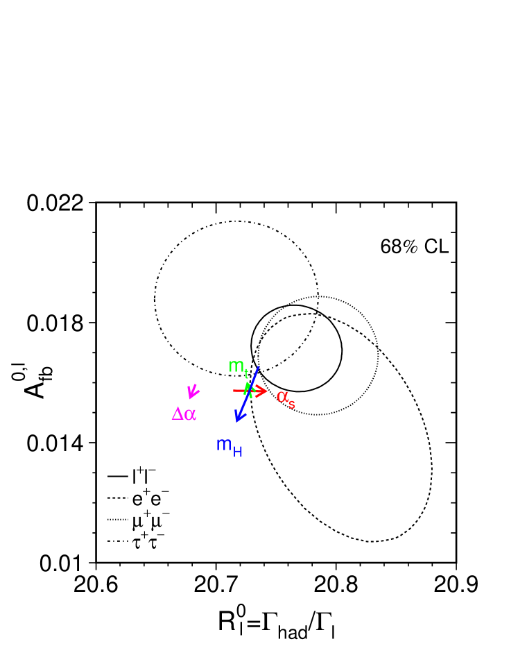
Figure 2.1: Contours of 68% probability in the $R^{0}_{\ell}$-$A^{0,\,\ell}_{\mathrm{FB}}$ plane. For better comparison the results for the $\tau$ lepton are corrected to correspond to the massless case. The Standard Model prediction for $m_{\mathrm{Z}}=91.1875$ GeV, $m_{\mathrm{t}}=178.0$ GeV, $m_{\mathrm{H}}=300$ GeV, and $\alpha_{\mathrm{S}}(m_{\mathrm{Z}}^{2})=0.118$ is also shown. The lines with arrows correspond to the variation of the Standard Model prediction when $m_{\mathrm{t}}$, $m_{\mathrm{H}}$, $\alpha_{\mathrm{S}}(m_{\mathrm{Z}}^{2})$ and $\Delta\alpha_{\mathrm{had}}^{(5)}(m_{\mathrm{Z}}^{2})$ are varied in the intervals $m_{\mathrm{t}}=178.0\pm 4.3$ GeV, $m_{\mathrm{H}}=300^{+700}_{-186}\leavevmode\nobreak\ {\mathrm{Ge\kern-1.00006ptV}}$, $\alpha_{\mathrm{S}}(m_{\mathrm{Z}}^{2})=0.118\pm 0.002$ and $\Delta\alpha_{\mathrm{had}}^{(5)}(m_{\mathrm{Z}}^{2})=0.02761\pm 0.00036$, respectively. The arrows point in the direction of increasing values of $m_{\mathrm{t}}$, $m_{\mathrm{H}}$, $\alpha_{\mathrm{S}}$ and $\Delta\alpha_{\mathrm{had}}^{(5)}(m_{\mathrm{Z}}^{2})$.

Chapter 3 The $\tau$ Polarisation

Updates with respect to summer 2003:
Unchanged w.r.t. summer 2002: All experiments have published final results which enter the combination. The final combination procedure is used, the obtained averages are final.

The longitudinal $\tau$ polarisation $\cal{P}_{\tau}$ of $\tau$ pairs produced in $\mathrm{Z}$ decays is defined as

$${\cal P}_{\tau} \equiv \frac{\sigma_{\mathrm{R}}-\sigma_{\mathrm{L}}}{\sigma_{\mathrm{R}}+\sigma_{\mathrm{L}}}\,,$$ (3.1)

where $\sigma_{\mathrm{R}}$ and $\sigma_{\mathrm{L}}$ are the $\tau$-pair cross sections for the production of a right-handed and left-handed $\tau^{-}$, respectively. The distribution of ${\cal P}_{\tau}$ as a function of the polar scattering angle $\theta$ between the $\mathrm{e}^{-}$ and the $\tau^{-}$, at $\sqrt{s}=m_{\mathrm{Z}}$, is given by

$${\cal P}_{\tau}(\cos\theta) = -\frac{{\cal A}_{\tau}(1+\cos^{2}\theta)+2{\cal A}_{\mathrm{e}}\cos\theta}{1+\cos^{2}\theta+2{\cal A}_{\tau}{\cal A}_{\mathrm{e}}\cos\theta}\,,$$ (3.2)

with ${\cal A}_{\mathrm{e}}$ and ${\cal A}_{\tau}$ as defined in Equation (2.4). Equation (3.2) is valid for pure Z exchange. The effects of $\gamma$ exchange, $\gamma$-$\mathrm{Z}$ interference and electromagnetic radiative corrections in the initial and final states are taken into account in the experimental analyses. In particular, these corrections account for the $\sqrt{s}$ dependence of the $\tau$ polarisation, which is important because the off-peak data are included in the event samples for all experiments. When averaged over all production angles $\cal{P}_{\tau}$ is a measurement of ${\cal A}_{\tau}$. As a function of $\cos\theta$, $\cal{P}_{\tau}(\cos\theta)$ provides nearly independent determinations of both ${\cal A}_{\tau}$ and ${\cal A}_{\mathrm{e}}$, thus allowing a test of the universality of the couplings of the $\mathrm{Z}$ to $\mathrm{e}$ and $\tau$.

Each experiment makes separate ${\cal P}_{\tau}$ measurements using the five $\tau$ decay modes e$\nu\overline{\nu}$, $\mu\nu\overline{\nu}$, $\pi\nu$, $\rho\nu$ and $a_{1}\nu$[16, 17, 18, 19]. The $\rho\nu$ and $\pi\nu$ are the most sensitive channels, contributing weights of about $40\%$ each in the average. DELPHI and L3 also use an inclusive hadronic analysis. The combination is made using the results from each experiment already averaged over the $\tau$ decay modes.

3.1 Results

Tables 3.1 and 3.2 show the most recent results for ${\cal A}_{\tau}$ and ${\cal A}_{\mathrm{e}}$ obtained by the four LEP collaborations[16, 17, 18, 19] and their combination. Although the sizes of the event samples used by the four experiments are roughly equal, smaller errors are quoted by ALEPH. This is largely associated with the higher angular granularity of the ALEPH electromagnetic calorimeter. Common systematic errors arise from uncertainties in radiative corrections (decay radiation) in the $\pi\nu$ and $\rho\nu$ channels, and in the modelling of the $a_{1}$ decays[20]. These errors and their correlations need further investigation, but are already taken into account in the combination (see also Reference 18). The statistical correlation between the extracted values of ${\cal A}_{\tau}$ and ${\cal A}_{\mathrm{e}}$ is small ($\leq$ 5%).

The average values for ${\cal A}_{\tau}$ and ${\cal A}_{\mathrm{e}}$:

$${\cal A}_{\tau} = 0.1439\pm 0.0043$$ (3.3)

$${\cal A}_{\mathrm{e}} = 0.1498\pm 0.0049\,,$$ (3.4)

with a correlation of 0.012, are compatible, in good agreement with neutral-current lepton universality. This combination is performed including the small common systematic errors between ${\cal A}_{\tau}$ and ${\cal A}_{\mathrm{e}}$ within each experiment and between experiments. Assuming $\mathrm{e}$-$\tau$ universality, the values for ${\cal A}_{\tau}$ and ${\cal A}_{\mathrm{e}}$ can be combined. The combined result of ${\cal A}_{\tau}$ and ${\cal A}_{\mathrm{e}}$ is:

$${\cal A}_{\ell} = 0.1465\pm 0.0033\,,$$ (3.5)

where the error includes a systematic component of 0.0016.

Experiment		${\cal A}_{\tau}$
ALEPH	(90 - 95), final	$0.1451\pm 0.0052\pm 0.0029$
DELPHI	(90 - 95), final	$0.1359\pm 0.0079\pm 0.0055$
L3	(90 - 95), final	$0.1476\pm 0.0088\pm 0.0062$
OPAL	(90 - 95), final	$0.1456\pm 0.0076\pm 0.0057$
LEP Average	final	$0.1439\pm 0.0035\pm 0.0026$

Table 3.1: LEP results for ${\cal A}_{\tau}$. The first error is statistical and the second systematic.

Experiment		${\cal A}_{\mathrm{e}}$
ALEPH	(90 - 95), final	$0.1504\pm 0.0068\pm 0.0008$
DELPHI	(90 - 95), final	$0.1382\pm 0.0116\pm 0.0005$
L3	(90 - 95), final	$0.1678\pm 0.0127\pm 0.0030$
OPAL	(90 - 95), final	$0.1454\pm 0.0108\pm 0.0036$
LEP Average	final	$0.1498\pm 0.0048\pm 0.0009$

Table 3.2: LEP results for ${\cal A}_{\mathrm{e}}$. The first error is statistical and the second systematic.

Chapter 4 Measurement of polarised lepton asymmetries at SLC

Updates with respect to summer 2003:
Unchanged w.r.t. summer 2000: SLD has published final results for $A_{\mathrm{LR}}$ and the leptonic left-right forward-backward asymmetries.

The measurement of the left-right cross section asymmetry ($A_{\mathrm{LR}}$) by SLD[21] at the SLC provides a systematically precise, statistics-dominated determination of the coupling ${\cal A}_{\mathrm{e}}$, and is presently the most precise single measurement, with the smallest systematic error, of this quantity. In principle the analysis is straightforward: one counts the numbers of Z bosons produced by left and right longitudinally polarised electrons, forms an asymmetry, and then divides by the luminosity-weighted e^- beam polarisation magnitude (the e⁺ beam is not polarised):

$$A_{\mathrm{LR}}=\frac{N_{\mathrm{L}}-N_{\mathrm{R}}}{N_{\mathrm{L}}+N_{\mathrm{R}}}\frac{1}{P_{\mathrm{e}}}.$$ (4.1)

Since the advent of high polarisation “strained lattice” GaAs photo-cathodes (1994), the average electron polarisation at the interaction point has been in the range 73% to 77%. The method requires no detailed final state event identification ($\mathrm{e}^{+}\mathrm{e}^{-}$ final state events are removed, as are non-Z backgrounds) and is insensitive to all acceptance and efficiency effects. The small total systematic error of 0.64% relative is dominated by the 0.50% relative systematic error in the determination of the e^- polarisation. The relative statistical error on $A_{\mathrm{LR}}$ is about 1.3%.

The precision Compton polarimeter detects beam electrons that are scattered by photons from a circularly polarised laser. Two additional polarimeters that are sensitive to the Compton-scattered photons and which are operated in the absence of positron beam, have verified the precision polarimeter result and are used to set a calibration uncertainty of 0.4% relative. In 1998, a dedicated experiment was performed in order to test directly the expectation that accidental polarisation of the positron beam was negligible; the e⁺ polarisation was found to be consistent with zero ($-0.02\pm 0.07$)%.

The $A_{\mathrm{LR}}$ analysis includes several very small corrections. The polarimeter result is corrected for higher order QED and accelerator related effects, a total of ($-0.22\pm 0.15$)% relative for 1997/98 data. The event asymmetry is corrected for backgrounds and accelerator asymmetries, a total of ($+0.15\pm 0.07$)% relative, for 1997/98 data.

The translation of the $A_{\mathrm{LR}}$ result to a “pole” value is a ($-2.5\pm 0.4$)% relative shift, where the uncertainty arises from the precision of the centre-of-mass energy determination. This small error due to the beam energy measurement reflects the results of a scan of the Z peak used to calibrate the energy spectrometers to $m_{\mathrm{Z}}$ from LEP data. The pole value, $A^{0}_{\mathrm{LR}}$, is equivalent to a measurement of ${\cal A}_{\mathrm{e}}$.

The 2000 result is included in a running average of all of the SLD $A_{\mathrm{LR}}$ measurements (1992, 1993, 1994/1995, 1996, 1997 and 1998). This updated result for $A^{0}_{\mathrm{LR}}$ (${\cal A}_{\mathrm{e}}$) is $0.1514\pm 0.0022$. In addition, the left-right forward-backward asymmetries for leptonic final states are measured[22]. From these, the parameters ${\cal A}_{\mathrm{e}}$, ${\cal A}_{\mu}$ and ${\cal A}_{\tau}$ can be determined. The results are ${\cal A}_{\mathrm{e}}=0.1544\pm 0.0060$, ${\cal A}_{\mu}=0.142\pm 0.015$ and ${\cal A}_{\tau}=0.136\pm 0.015$. The lepton-based result for ${\cal A}_{\mathrm{e}}$ can be combined with the $A^{0}_{\mathrm{LR}}$ result to yield ${\cal A}_{\mathrm{e}}=0.1516\pm 0.0021$, including small correlations in the systematic errors. The correlation of this measurement with ${\cal A}_{\mu}$ and ${\cal A}_{\tau}$ is indicated in Table 4.1.

Assuming lepton universality, the $A_{\mathrm{LR}}$ result and the results on the leptonic left-right forward-backward asymmetries can be combined, while accounting for small correlated systematic errors, yielding

$${\cal A}_{\ell}=0.1513\pm 0.0021.$$ (4.2)

	${\cal A}_{\mathrm{e}}$	${\cal A}_{\mu}$	${\cal A}_{\tau}$
${\cal A}_{\mathrm{e}}$	1.000
${\cal A}_{\mu}$	0.038	1.000
${\cal A}_{\tau}$	0.033	0.007	1.000

Table 4.1: Correlation coefficients between ${\cal A}_{\mathrm{e}}$, ${\cal A}_{\mu}$ and ${\cal A}_{\tau}$

Chapter 5 Results from b and c Quarks

Updates with respect to summer 2003:
All experimental inputs are final, although some publications are pending. The combination is still preliminary.

5.1 Introduction

The relevant quantities in the heavy quark sector at LEP-I/SLD which are currently determined by the combination procedure are:

• The ratios of the b and c quark partial widths of the Z to its total hadronic partial width: $R_{\mathrm{b}}^{0}\equiv\Gamma_{\mathrm{b\overline{b}}}/\Gamma_{\mathrm{had}}$ and $R_{\mathrm{c}}^{0}\equiv\Gamma_{\mathrm{c\overline{c}}}/\Gamma_{\mathrm{had}}$. (The symbols $R_{\mathrm{b}}$, $R_{\mathrm{c}}$ are used to denote the experimentally measured ratios of event rates or cross sections.)

• The forward-backward asymmetries, $A_{\mathrm{FB}}^{\mathrm{b\overline{b}}}$ and $A_{\mathrm{FB}}^{\mathrm{c\overline{c}}}$.

• The final state coupling parameters ${\cal A}_{\mathrm{b}},\,{\cal A}_{\mathrm{c}}$ obtained from the left-right-forward-backward asymmetry at SLD.

• The semileptonic branching ratios, $\mathrm{BR}(\rm b\rightarrow\ell^{-})$, $\mathrm{BR}(\mathrm{b\rightarrow c\rightarrow\ell^{+}})$ and $\mathrm{BR}(\mathrm{c}\rightarrow\ell^{+})$, and the average time-integrated ${\rm B}^{0}{\overline{{\rm B}^{0}}}$ mixing parameter, $\overline{\chi}$. These are often determined at the same time or with similar methods as the asymmetries. Including them in the combination greatly reduces the errors. For example $\overline{\chi}$ parameterises the probability that a b-quark decays into a negative lepton which is the charge tagging efficiency in the asymmetry analyses. For this reason the errors coming from the mixture of different lepton sources in $\mathrm{b\overline{b}}$ events cancel largely in the asymmetries if they are analyses together with $\overline{\chi}$.

• The probability that a c quark produces a ${\rm D}^{+}$, ${\rm{D_{s}}}$, ${\rm D}^{*+}$ meson or a charmed baryon. The probability that a c quark fragments into a ${\rm D}^{0}$ is calculated from the constraint that the probabilities for the weakly decaying charmed hadrons add up to one.

A full description of the averaging procedure is published in [3]; the main motivations for the procedure are outlined here. Several analyses measure more than one parameter simultaneously, for example the asymmetry measurements with leptons or D mesons. Some of the measurements of electroweak parameters depend explicitly on the values of other parameters, for example $R_{\mathrm{b}}$ depends on $R_{\mathrm{c}}$. The common tagging and analysis techniques lead to common sources of systematic uncertainty, in particular for the double-tag measurements of $R_{\mathrm{b}}$. The starting point for the combination is to ensure that all the analyses use a common set of assumptions for input parameters which give rise to systematic uncertainties. The input parameters are updated and extended [23] to accommodate new analyses and more recent measurements. The correlations and interdependencies of the input measurements are then taken into account in a $\chi^{2}$ minimisation which results in the combined electroweak parameters and their correlation matrix.

5.2 Summary of Measurements and Averaging Procedure

All measurements are presented by the LEP and SLD collaborations in a consistent manner for the purpose of combination. The tables prepared by the experiments include a detailed breakdown of the systematic error of each measurement and its dependence on other electroweak parameters. Where necessary, the experiments apply small corrections to their results in order to use agreed values and ranges for the input parameters to calculate systematic errors. The measurements, corrected where necessary, are summarised in Appendix A in Tables A.1–A.20, where the statistical and systematic errors are quoted separately. The correlated systematic entries are from physics sources shared with one or more other results in the tables and are derived from the full breakdown of common systematic uncertainties. The uncorrelated systematic entries come from the remaining sources.

5.2.1 Averaging Procedure

A $\chi^{2}$ minimisation procedure is used to derive the values of the heavy-flavour electroweak parameters, following the procedure described in Reference 3. The full statistical and systematic covariance matrix for all measurements is calculated. This correlation matrix takes into account correlations between different measurements of one experiment and between different experiments. The explicit dependence of each measurement on the other parameters is also accounted for.

Since c-quark events form the main background in the $R_{\mathrm{b}}$ analyses, the value of $R_{\mathrm{b}}$ depends on the value of $R_{\mathrm{c}}$. If $R_{\mathrm{b}}$ and $R_{\mathrm{c}}$ were measured in the same analysis, this would be reflected in the correlation matrix for the results. However the analyses do not determine $R_{\mathrm{b}}$ and $R_{\mathrm{c}}$ simultaneously but instead measure $R_{\mathrm{b}}$ for an assumed value of $R_{\mathrm{c}}$. In this case the dependence is parameterised as

$$R_{\mathrm{b}} = R_{\mathrm{b}}^{\rm{meas}}+a(R_{\mathrm{c}})\frac{(R_{\mathrm{c}}-R_{\mathrm{c}}^{\rm{used}})}{R_{\mathrm{c}}}.$$ (5.1)

In this expression, $R_{\mathrm{b}}^{\rm{meas}}$ is the result of the analysis assuming a value of $R_{\mathrm{c}}=R_{\mathrm{c}}^{\rm{used}}$. The values of $R_{\mathrm{c}}^{\rm{used}}$ and the coefficients $a(R_{\mathrm{c}})$ are given in Table A.1 where appropriate. The dependence of all other measurements on other electroweak parameters is treated in the same way, with coefficients $a(x)$ describing the dependence on parameter $x$.

5.2.2 Partial Width Measurements

The measurements of $R_{\mathrm{b}}$ and $R_{\mathrm{c}}$ fall into two categories. In the first, called a single-tag measurement, a method to select b or c events is devised, and the number of tagged events is counted. This number must then be corrected for backgrounds from other flavours and for the tagging efficiency to calculate the true fraction of hadronic $\mathrm{Z}$ decays of that flavour. The dominant systematic errors come from understanding the branching ratios and detection efficiencies which give the overall tagging efficiency. For the second technique, called a double-tag measurement, each event is divided into two hemispheres. With $N_{t}$ being the number of tagged hemispheres, $N_{tt}$ the number of events with both hemispheres tagged and $N_{\rm{had}}$ the total number of hadronic $\mathrm{Z}$ decays one has

$$\frac{N_{t}}{2N_{\rm{had}}} = \varepsilon_{\mathrm{b}}R_{\mathrm{b}}+\varepsilon_{\mathrm{c}}R_{\mathrm{c}}+\varepsilon_{\mathrm{uds}}(1-R_{\mathrm{b}}-R_{\mathrm{c}}),$$ (5.2)

$$\frac{N_{tt}}{N_{\rm{had}}} = {\cal C}_{\rm b}\varepsilon_{\mathrm{b}}^{2}R_{\mathrm{b}}+{\cal C}_{\rm c}\varepsilon_{\mathrm{c}}^{2}R_{\mathrm{c}}+{\cal C}_{\mathrm{uds}}\varepsilon_{\mathrm{uds}}^{2}(1-R_{\mathrm{b}}-R_{\mathrm{c}}),$$ (5.3)

where $\varepsilon_{\mathrm{b}}$, $\varepsilon_{\mathrm{c}}$ and $\varepsilon_{\mathrm{uds}}$ are the tagging efficiencies per hemisphere for b, c and light-quark events, and ${\cal C}_{\rm q}\neq 1$ accounts for the fact that the tagging efficiencies between the hemispheres may be correlated. In the case of $R_{\mathrm{b}}$ one has $\varepsilon_{\mathrm{b}}\gg\varepsilon_{\mathrm{c}}\gg\varepsilon_{\mathrm{uds}}$, ${\cal C}_{\rm b}\approx 1$. The correlations for the other flavours can be neglected. These equations can be solved to give $R_{\mathrm{b}}$ and $\varepsilon_{\mathrm{b}}$. Neglecting the c and uds backgrounds and the correlations, they are approximately given by

$$\varepsilon_{\mathrm{b}} \approx 2N_{tt}/N_{t},$$ (5.4)

$$R_{\mathrm{b}} \approx N_{t}^{2}/(4N_{tt}N_{\rm{had}}).$$ (5.5)

The double-tagging method has the advantage that the b tagging efficiency is derived from the data, reducing the systematic error. The residual background of other flavours in the sample, and the evaluation of the correlation between the tagging efficiencies in the two hemispheres of the event are the main sources of systematic uncertainty in such an analysis.

In the standard approach each hemisphere is simply tagged as b or non-b. This method can be enhanced by using more tags. All additional efficiencies can be determined from the data, reducing the statistical uncertainties without adding new systematic uncertainties.

Small corrections must be applied to the results to obtain the partial width ratios $R_{\mathrm{b}}^{0}$ and $R_{\mathrm{c}}^{0}$ from the cross section ratios $R_{\mathrm{b}}$ and $R_{\mathrm{c}}$. These corrections depend slightly on the invariant mass cutoff of the simulations used by the experiments; they are applied by the collaborations before the combination.

The partial width measurements included are:

• Lifetime (and lepton) double-tag measurements for $R_{\mathrm{b}}$ from ALEPH[24], DELPHI[25], L3[26], OPAL[27] and SLD[28]. These are the most precise determinations of $R_{\mathrm{b}}$. Since they completely dominate the combined result, no other $R_{\mathrm{b}}$ measurements are used at present. The basic features of the double-tag technique are discussed above. In the ALEPH, DELPHI, OPAL and SLD measurements the charm rejection is enhanced by using the invariant mass information. DELPHI, OPAL and SLD also add kinematic information from the particles at the secondary vertex. The ALEPH and DELPHI measurements make use of several different tags, which significantly reduces the statistical error. This in turn allows a harder cut on the primary b-tag to be used, leading to a higher b-purity and a corresponding reduction in the systematic error.

• Analyses with D/${\mathrm{D}}^{*\pm}$ mesons to measure $R_{\mathrm{c}}$ from ALEPH, DELPHI and OPAL. All measurements are constructed in such a way that no assumptions about charm fragmentation are necessary as these are determined from the LEP-I data. The available measurements can be divided into three groups:

  • inclusive/exclusive double tag (ALEPH[29], DELPHI[30, 31], OPAL[32]): In a first step ${\mathrm{D}}^{*\pm}$ mesons are reconstructed in the decay channel ${\rm D}^{*+}\rightarrow\pi^{+}{\rm D}^{0}$ using several decay channels of the ${\rm D}^{0}$ and their production rate is measured, which depends on the product $R_{\mathrm{c}}\times\mathrm{P(c\rightarrow D^{*+})}\times\mathrm{BR(D^{*+}\rightarrow\pi^{+}D^{0})}$. This sample of $\mathrm{c\overline{c}}$ (and $\mathrm{b\overline{b}}$) events is then used to measure $\mathrm{P(c\rightarrow D^{*+})}\times\mathrm{BR(D^{*+}\rightarrow\pi^{+}D^{0})}$ using a slow pion tag in the opposite hemisphere. In the ALEPH measurement only $R_{\mathrm{c}}$ is given and no explicit $\mathrm{P(c\rightarrow D^{*+})}\times\mathrm{BR(D^{*+}\rightarrow\pi^{+}D^{0})}$ is available.

  • exclusive double tag (ALEPH[29]): This analysis uses exclusively reconstructed ${\rm D}^{*+}$, ${\rm D}^{0}$ and ${\rm D}^{+}$ mesons in different decay channels. It has lower statistics but better purity than the inclusive analyses.

  • reconstruction of all weakly decaying charmed states (ALEPH[33], DELPHI[31], OPAL[34]): These analyses make the assumption that the production fractions of ${\rm D}^{0}$, ${\rm D}^{+}$, ${\rm{D_{s}}}$ and ${\rm{\Lambda_{c}}}$ in c-quark jets of $\mathrm{c\overline{c}}$ events add up to one with small corrections due to unmeasured charmed strange baryons. This is a single tag measurement, relying only on knowing the decay branching ratios of the charm hadrons. These analyses are also used to measure the c hadron production ratios which are needed for the $R_{\mathrm{b}}$ analyses.

• A lifetime plus mass double tag from SLD to measure $R_{\mathrm{c}}$[35]. This analysis uses the same tagging algorithm as the SLD $R_{\mathrm{b}}$ analysis, but with the neural net tuned to tag charm. Although the charm tag has a purity of about 84%, most of the background is from b which can be measured with high precision from the b/c mixed tag rate.

• A measurement of $R_{\mathrm{c}}$ using single leptons assuming $\mathrm{BR}(\mathrm{c}\rightarrow\ell^{+})$ from ALEPH [29].

To avoid effects from nonlinearities in the fit, for the inclusive/exclusive single/double tag and for the charm-counting analyses, the products $\mathrm{R_{c}P(c\rightarrow D^{*+})\times BR(D^{*+}\rightarrow\pi^{+}D^{0})}$, ${\rm{R_{c}f_{D^{0}}}}$, ${\rm{R_{c}f_{D^{+}}}}$, ${\rm{R_{c}f_{D_{s}}}}$ and ${\rm{R_{c}f_{\Lambda_{c}}}}$that are actually measured in the analyses are directly used as inputs to the fit. The measurements of the production rates of weakly decaying charmed hadrons, especially ${\rm{R_{c}f_{D_{s}}}}$ and ${\rm{R_{c}f_{\Lambda_{c}}}}$ have substantial errors due to the uncertainties in the branching ratios of the decay mode used. These errors are relative so that the absolute errors are smaller when the measurements fluctuate downwards, leading to a potential bias towards lower averages. To avoid this bias, for the production rates of weakly decaying charmed hadrons the logarithm of the production rates instead of the rates themselves are input to the fit. For ${\rm{R_{c}f_{D^{0}}}}$ and ${\rm{R_{c}f_{D^{+}}}}$ the difference between the results using the logarithm or the value itself is negligible. For ${\rm{R_{c}f_{D_{s}}}}$ and ${\rm{R_{c}f_{\Lambda_{c}}}}$ the difference in the extracted value of $R_{\mathrm{c}}$ is about one tenth of a standard deviation.

5.2.3 Asymmetry Measurements

All b and c asymmetries given by the experiments correspond to full acceptance.

The QCD corrections to the forward-backward asymmetries depend strongly on the experimental analyses. For this reason the numbers given by the collaborations are also corrected for QCD effects. A detailed description of the procedure can be found in [36] with updates reported in [23].

For the heavy-flavour combinations described in this chapter, the LEP peak and off-peak asymmetries are corrected to $\sqrt{s}=91.26$ GeV using the predicted dependence from ZFITTER[37]. The slope of the asymmetry around $m_{\mathrm{Z}}$ depends only on the axial coupling and the charge of the initial and final state fermions and is thus independent of the value of the asymmetry itself, i.e., the effective electroweak mixing angle.

After calculating the overall averages, the quark pole asymmetries $A^{0,\,{\mathrm{q}}}_{\mathrm{FB}}$, defined in terms of effective couplings, are derived from the measured asymmetries by applying corrections as listed in Table 5.1. These corrections are due to the energy shift from 91.26 GeV to $m_{\mathrm{Z}}$, initial state radiation, $\gamma$ exchange and $\gamma$-$\mathrm{Z}$ interference. A very small correction due to the nonzero value of the b quark mass is included in the last correction. All corrections are calculated using ZFITTER. Recently, a small inconsistency was discovered in the treatment of b-quarks for the latest sets of raditive corrections in ZFITTER. To account for these inconsistencies a systematic error of 0.0005 is added to $A^{0,\,{\mathrm{b}}}_{\mathrm{FB}}$.

Source	$\delta A_{\mathrm{FB}}^{\mathrm{b}}$	$\delta A_{\mathrm{FB}}^{\mathrm{c}}$
$\sqrt{s}=m_{\mathrm{Z}}$	$-0.0013$	$-0.0034$
QED corrections	$+0.0041$	$+0.0104$
$\gamma$, $\gamma$-$\mathrm{Z}$, mass	$-0.0003$	$-0.0008$
Total	$+0.0025$	$+0.0062$

Table 5.1: Corrections to be applied to the quark asymmetries as $A_{\mathrm{FB}}^{0}=A_{\mathrm{FB}}^{\mathrm{meas}}+\delta A_{\mathrm{FB}}$.

The SLD left-right-forward-backward asymmetries are also corrected for all radiative effects and are directly presented in terms of ${\cal A}_{\mathrm{b}}$ and ${\cal A}_{\mathrm{c}}$.

The measurements used are:

• Measurements of $A_{\mathrm{FB}}^{\mathrm{b\overline{b}}}$ and $A_{\mathrm{FB}}^{\mathrm{c\overline{c}}}$ using leptons from ALEPH[39], DELPHI[40], L3[41] and OPAL[42]. These analyses measure either $A_{\mathrm{FB}}^{\mathrm{b\overline{b}}}$ only or $A_{\mathrm{FB}}^{\mathrm{b\overline{b}}}$ and $A_{\mathrm{FB}}^{\mathrm{c\overline{c}}}$ from a fit to the lepton spectra. In the case of OPAL the lepton information is combined with hadronic variables in a neural net. DELPHI uses in addition lifetime information and jet-charge in the hemisphere opposite to the lepton to separate the different lepton sources. Some asymmetry analyses also measure $\overline{\chi}$ within the same analysis.

• Measurements of $A_{\mathrm{FB}}^{\mathrm{b\overline{b}}}$ based on lifetime tagged events with a hemisphere charge measurement from ALEPH[43], DELPHI[44], L3[45] and OPAL[46]. These measurements dominate the combined result.

• Analyses with D mesons to measure $A_{\mathrm{FB}}^{\mathrm{c\overline{c}}}$ from ALEPH[47] or $A_{\mathrm{FB}}^{\mathrm{c\overline{c}}}$ and $A_{\mathrm{FB}}^{\mathrm{b\overline{b}}}$ from DELPHI[48] and OPAL[49].

• Measurements of ${\cal A}_{\mathrm{b}}$ and ${\cal A}_{\mathrm{c}}$ from SLD. These results include measurements using lepton [50], D meson [51] and vertex mass plus hemisphere charge [52] tags, which have similar sources of systematic errors as the LEP asymmetry measurements. SLD also uses vertex mass for bottom or charm tagging in conjunction with a kaon tag or a vertex charge tag for both ${\cal A}_{\mathrm{b}}$ and ${\cal A}_{\mathrm{c}}$ measurements [53, 54].

Since all asymmetry measurements use the full event sample the analyses using different techniques from the same collaboration are statistically correlated. These correlations are evaluated by the experiments and included in the combination procedure. The correlations between the b-asymmetry measurements with jetcharge and with leptons range between 6% and 30%.

5.2.4 Other Measurements

The measurements of the charmed hadron fractions $\mathrm{P(c\rightarrow D^{*+})}\times\mathrm{BR(D^{*+}\rightarrow\pi^{+}D^{0})}$, $f({\rm D}^{+})$, $f({\rm{D_{s}}})$ and $f({\mathrm{c_{baryon}}})$ are included in the $R_{\mathrm{c}}$ measurements and are described there.

ALEPH[55], DELPHI[56], L3[57, 26] and OPAL[58] measure $\mathrm{BR}(\rm b\rightarrow\ell^{-})$, $\mathrm{BR}(\mathrm{b\rightarrow c\rightarrow\ell^{+}})$ and $\overline{\chi}$ or a subset of them from a sample of leptons opposite to a b-tagged hemisphere and from a double lepton sample. DELPHI[30] and OPAL[59] measure $\mathrm{BR}(\mathrm{c}\rightarrow\ell^{+})$ from a sample opposite to a high energy ${\mathrm{D}}^{*\pm}$.

5.3 Results

In a first fit the asymmetry measurements on peak, above peak and below peak are corrected to three common centre-of-mass energies and are then combined at each energy point. The results of this fit, including the SLD results, are given in Appendix B. The dependence of the average asymmetries on centre-of-mass energy agrees with the prediction of the Standard Model, as shown in Figure 5.1. A second fit is made to derive the pole asymmetries $A^{0,\,{\mathrm{q}}}_{\mathrm{FB}}$ from the measured quark asymmetries, in which all the off-peak asymmetry measurements are corrected to the peak energy before combining. This fit determines a total of 14 parameters: the two partial widths, two LEP asymmetries, two coupling parameters from SLD, three semileptonic branching ratios, the average mixing parameter and the probabilities for c quark to fragment into a ${\rm D}^{+}$, a ${\rm{D_{s}}}$, a ${\rm D}^{*+}$, or a charmed baryon. If the SLD measurements are excluded from the fit there are 12 parameters to be determined. Results for the non-electroweak parameters are independent of the treatment of the off-peak asymmetries and the SLD data.

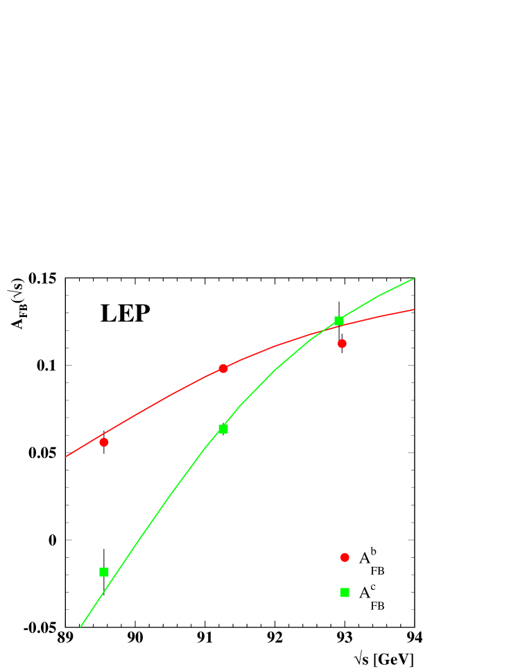
Figure 5.1: Measured asymmetries for b and c quark final states as a function of the centre-of-mass energy. The Standard-Model expectations are shown as the lines calculated for $m_{\mathrm{t}}=175\leavevmode\nobreak\ {\mathrm{Ge\kern-1.00006ptV}}$ and $m_{\mathrm{H}}=300\leavevmode\nobreak\ {\mathrm{Ge\kern-1.00006ptV}}$.

5.3.1 Results of the 12-Parameter Fit to the LEP Data

Using the full averaging procedure gives the following combined results for the electroweak parameters:

$$R_{\mathrm{b}}^{0} = 0.21643\pm 0.00073$$ (5.6)

$$R_{\mathrm{c}}^{0} = 0.1691\pm 0.0047$$

$$A^{0,\,{\mathrm{b}}}_{\mathrm{FB}} = 0.0998\pm 0.0017$$

$$A^{0,\,{\mathrm{c}}}_{\mathrm{FB}} = 0.0702\pm 0.0035\,,$$

where all corrections to the asymmetries and partial widths are applied. The $\chi^{2}/$d.o.f. is $49/(96-12)$. The corresponding correlation matrix is given in Table 5.2.

	$R_{\mathrm{b}}^{0}$	$R_{\mathrm{c}}^{0}$	$A^{0,\,{\mathrm{b}}}_{\mathrm{FB}}$	$A^{0,\,{\mathrm{c}}}_{\mathrm{FB}}$
$R_{\mathrm{b}}^{0}$	$1.00$	$-0.17$	$-0.11$	$0.08$
$R_{\mathrm{c}}^{0}$	$-0.17$	$1.00$	$0.05$	$-0.06$
$A^{0,\,{\mathrm{b}}}_{\mathrm{FB}}$	$-0.11$	$0.05$	$1.00$	$0.15$
$A^{0,\,{\mathrm{c}}}_{\mathrm{FB}}$	$0.08$	$-0.06$	$0.15$	$1.00$

Table 5.2: The correlation matrix for the four electroweak parameters from the 12-parameter fit.

5.3.2 Results of the 14-Parameter Fit to LEP and SLD Data

Including the SLD results for $R_{\mathrm{b}}$, $R_{\mathrm{c}}$, ${\cal A}_{\mathrm{b}}$ and ${\cal A}_{\mathrm{c}}$ into the fit the following results are obtained:

$$R_{\mathrm{b}}^{0} = 0.21630\pm 0.00066\,,$$ (5.7)

$$R_{\mathrm{c}}^{0} = 0.1723\pm 0.0031\,,$$

$$A^{0,\,{\mathrm{b}}}_{\mathrm{FB}} = 0.0998\pm 0.0017\,,$$

$$A^{0,\,{\mathrm{c}}}_{\mathrm{FB}} = 0.0706\pm 0.0035\,,$$

$${\cal A}_{\mathrm{b}} = 0.923\pm 0.020\,,$$

$${\cal A}_{\mathrm{c}} = 0.670\pm 0.027\,,$$

with a $\chi^{2}/$d.o.f. of $53/(105-14)$. The corresponding correlation matrix is given in Table 5.3 and the largest errors for the electroweak parameters are listed in Table 5.4. As a cross check the fit has been repeated using statistical errors only, resulting in consistent central values and a $\chi^{2}/$d.o.f. of $92/(105-14)$. In this case a large contribution to the $\chi^{2}$ comes from $\mathrm{BR}(\rm b\rightarrow\ell^{-})$ measurements, which is sharply reduced when detector systematics are included. Subtracting the $\chi^{2}$ contribution from $\mathrm{BR}(\rm b\rightarrow\ell^{-})$ measurements one gets $\chi^{2}/{\rm d.o.f.}=65/(99-13)$. This shows that the low $\chi^{2}$ largely comes from a statistical fluctuation. In addition many systematic errors are estimated very conservatively. Several error sources are evaluated by comparing test quantities between data and simulation. The statistical errors of these tests are taken as systematic uncertainties but no correction is applied, since one has good reasons to believe that the Monte Carlo describes the truth better than suggested by the test. Also in some cases, such as for the $\rm b\rightarrow\ell^{-}$ model fairly conservative assumptions are used for the error evaluation which are extreme enough to be clearly incompatible with the data. However it should be noted that especially for the quark forward backward asymmetries the systematic errors are much smaller than the statistical ones so that a possible overestimate of these errors cannot hide disagreements with other electroweak measurements.

In deriving these results the parameters ${\cal A}_{\mathrm{b}}$ and ${\cal A}_{\mathrm{c}}$ are treated as independent of the forward-backward asymmetries $A^{0,\,{\mathrm{b}}}_{\mathrm{FB}}$ and $A^{0,\,{\mathrm{c}}}_{\mathrm{FB}}$ (but see Section 15.1 for a joint analysis). In Figure 5.2 the results for $R_{\mathrm{b}}^{0}$ and $R_{\mathrm{c}}^{0}$ are shown compared with the Standard Model expectation.

	$R_{\mathrm{b}}^{0}$	$R_{\mathrm{c}}^{0}$	$A^{0,\,{\mathrm{b}}}_{\mathrm{FB}}$	$A^{0,\,{\mathrm{c}}}_{\mathrm{FB}}$	${\cal A}_{\mathrm{b}}$	${\cal A}_{\mathrm{c}}$
$R_{\mathrm{b}}^{0}$	$1.00$	$-0.18$	$-0.10$	$0.07$	$-0.08$	$0.04$
$R_{\mathrm{c}}^{0}$	$-0.18$	$1.00$	$0.04$	$-0.06$	$0.04$	$-0.06$
$A^{0,\,{\mathrm{b}}}_{\mathrm{FB}}$	$-0.10$	$0.04$	$1.00$	$0.15$	$0.06$	$0.01$
$A^{0,\,{\mathrm{c}}}_{\mathrm{FB}}$	$0.07$	$-0.06$	$0.15$	$1.00$	$-0.02$	$0.04$
${\cal A}_{\mathrm{b}}$	$-0.08$	$0.04$	$0.06$	$-0.02$	$1.00$	$0.11$
${\cal A}_{\mathrm{c}}$	$0.04$	$-0.06$	$0.01$	$0.04$	$0.11$	$1.00$

Table 5.3: The correlation matrix for the six electroweak parameters from the 14-parameter fit.

	$R_{\mathrm{b}}^{0}$	$R_{\mathrm{c}}^{0}$	$A^{0,\,{\mathrm{b}}}_{\mathrm{FB}}$	$A^{0,\,{\mathrm{c}}}_{\mathrm{FB}}$	${\cal A}_{\mathrm{b}}$	${\cal A}_{\mathrm{c}}$
	$(10^{-3})$	$(10^{-3})$	$(10^{-3})$	$(10^{-3})$	$(10^{-2})$	$(10^{-2})$
statistics	$0.44$	$2.4$	$1.4$	$3.0$	$1.5$	$2.2$
internal systematics	$0.28$	$1.2$	$0.4$	$1.4$	$1.2$	$1.5$
QCD effects	$0.18$	$\mathrm{𝟎}$	$0.4$	$0.1$	$0.3$	$0.2$
BR(D $\rightarrow$ neut.)	$0.13$	$0.3$	$\mathrm{𝟎}$	$\mathrm{𝟎}$	$\mathrm{𝟎}$	$\mathrm{𝟎}$
D decay multiplicity	$0.13$	$0.6$	$\mathrm{𝟎}$	$0.2$	$\mathrm{𝟎}$	$\mathrm{𝟎}$
B decay multiplicity	$0.11$	$\mathrm{𝟎}$	$\mathrm{𝟎}$	$0.2$	$\mathrm{𝟎}$	$\mathrm{𝟎}$
BR(D${}^{+}\rightarrow$ K${}^{-}\pi^{+}\pi^{+})$	$0.09$	$0.2$	$\mathrm{𝟎}$	$0.1$	$\mathrm{𝟎}$	$\mathrm{𝟎}$
BR(${\rm{D_{s}}}\rightarrow\phi\pi^{+})$	$0.02$	$0.5$	$\mathrm{𝟎}$	$0.1$	$\mathrm{𝟎}$	$\mathrm{𝟎}$
BR($\Lambda_{\mathrm{c}}\rightarrow$p K${}^{-}\pi^{+})$	$0.05$	$0.5$	$\mathrm{𝟎}$	$0.1$	$\mathrm{𝟎}$	$\mathrm{𝟎}$
D lifetimes	$0.07$	$0.6$	$\mathrm{𝟎}$	$0.2$	$\mathrm{𝟎}$	$\mathrm{𝟎}$
B decays	$\mathrm{𝟎}$	$\mathrm{𝟎}$	$0.1$	$0.4$	$\mathrm{𝟎}$	$0.1$
decay models	$\mathrm{𝟎}$	$0.1$	$0.1$	$0.5$	$0.1$	$0.1$
non incl. mixing	$\mathrm{𝟎}$	$0.1$	$0.1$	$0.4$	$\mathrm{𝟎}$	$\mathrm{𝟎}$
gluon splitting	$0.23$	$0.9$	$0.1$	$0.2$	$0.1$	$0.1$
c fragmentation	$0.11$	$0.3$	$0.1$	$0.1$	$0.1$	$0.1$
light quarks	$0.07$	$0.1$	$\mathrm{𝟎}$	$0.3$	$\mathrm{𝟎}$	$\mathrm{𝟎}$
beam polarisation	$\mathrm{𝟎}$	$\mathrm{𝟎}$	$\mathrm{𝟎}$	$\mathrm{𝟎}$	$0.5$	$0.3$
ZFITTER corrections	$\mathrm{𝟎}$	$\mathrm{𝟎}$	$0.5$	$\mathrm{𝟎}$	$\mathrm{𝟎}$	$\mathrm{𝟎}$
total correlated	$0.42$	$1.5$	$0.6$	$0.9$	$0.6$	$0.4$
total error	$0.66$	$3.1$	$1.7$	$3.5$	$2.0$	$2.7$

Table 5.4: The dominant error sources for the electroweak parameters from the 14-parameter fit.

Amongst the non-electroweak observables the B semileptonic branching fraction ($\mbox{$\mathrm{BR}(\rm b\rightarrow\ell^{-})$}\,=\,0.1071\pm 0.0022$) is of special interest. The dominant error source on this quantity is the dependence on the semileptonic decay models $\rm b\rightarrow\ell^{-}$, $\mathrm{c}\rightarrow\ell^{+}$ with

$$\Delta\mbox{$\mathrm{BR}(\rm b\rightarrow\ell^{-})$}_{\rm b\rightarrow\ell^{-}-\rm{modelling}}=0.0012.$$ (5.8)

Extensive studies have been made to understand the size of this error. Amongst the electroweak quantities the quark asymmetries with leptons depend also on the assumptions on the decay model while the asymmetries using other methods usually do not. The fit implicitly requires that the different methods give consistent results. This effectively constrains the decay model and thus reduces the error from this source in the fit result for $\mathrm{BR}(\rm b\rightarrow\ell^{-})$.

To get a conservative estimate of the modelling error in $\mathrm{BR}(\rm b\rightarrow\ell^{-})$ the fit is repeated removing all asymmetry measurements. The result of this fit is

$$\mbox{$\mathrm{BR}(\rm b\rightarrow\ell^{-})$}\,=\,0.1069\pm 0.0022$$ (5.9)

with

$$\Delta\mbox{$\mathrm{BR}(\rm b\rightarrow\ell^{-})$}_{\rm b\rightarrow\ell^{-}-\rm{modelling}}=0.0013.$$ (5.10)

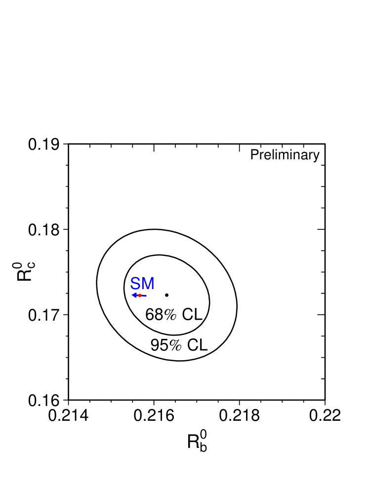
Figure 5.2: Contours in the ($R_{\mathrm{b}}^{0}$,$R_{\mathrm{c}}^{0}$) plane derived from the LEP+SLD data, corresponding to 68% and 95% confidence levels assuming Gaussian systematic errors. The Standard Model prediction for $m_{\mathrm{t}}=178.0\pm 4.3$ GeV is also shown. The arrow points in the direction of increasing values of $m_{\mathrm{t}}$.

Chapter 6 The Hadronic Charge Asymmetry ${\langle Q_{\mathrm{FB}}\rangle}$

Updates with respect to summer 2003:
Unchanged w.r.t. summer 2002: All experiments have published final results which enter the combination. The final combination procedure is used, the obtained averages are final.

The LEP experiments ALEPH[60], DELPHI[61], L3[45] and OPAL[62] provide measurements of the hadronic charge asymmetry based on the mean difference in jet charges measured in the forward and backward event hemispheres, ${\langle Q_{\mathrm{FB}}\rangle}$. DELPHI also provides a related measurement of the total charge asymmetry by making a charge assignment on an event-by-event basis and performing a likelihood fit[61]. The experimental values quoted for the average forward-backward charge difference, ${\langle Q_{\mathrm{FB}}\rangle}$, cannot be directly compared as some of them include detector dependent effects such as acceptances and efficiencies. Therefore the effective electroweak mixing angle, $\sin^{2}\theta_{\mathrm{eff}}^{\mathrm{lept}}$, as defined in Section 15.3, is used as a means of combining the experimental results summarised in Table 6.1.

Experiment		$\sin^{2}\theta_{\mathrm{eff}}^{\mathrm{lept}}$
ALEPH	(90-94), final	$0.2322\pm 0.0008\pm 0.0011$
DELPHI	(91-91), final	$0.2345\pm 0.0030\pm 0.0027$
L3	(91-95), final	$0.2327\pm 0.0012\pm 0.0013$
OPAL	(90-91), final	$0.2326\pm 0.0012\pm 0.0029$
LEP Average		$0.2324\pm 0.0012$

Table 6.1: Summary of the determination of $\sin^{2}\theta_{\mathrm{eff}}^{\mathrm{lept}}$ from inclusive hadronic charge asymmetries at LEP. For each experiment, the first error is statistical and the second systematic. The latter, amounting to 0.0010 in the average, is dominated by fragmentation and decay modelling uncertainties.

The dominant source of systematic error arises from the modelling of the charge flow in the fragmentation process for each flavour. All experiments measure the required charge properties for $\mathrm{Z}\rightarrow\mathrm{b\overline{b}}$ events from the data. ALEPH also determines the charm charge properties from the data. The fragmentation model implemented in the JETSET Monte Carlo program[63] is used by all experiments as reference; the one of the HERWIG Monte Carlo program[64] is used for comparison. The JETSET fragmentation parameters are varied to estimate the systematic errors. The central values chosen by the experiments for these parameters are, however, not the same. The smaller of the two fragmentation errors in any pair of results is treated as common to both. The present average of $\sin^{2}\theta_{\mathrm{eff}}^{\mathrm{lept}}$ from ${\langle Q_{\mathrm{FB}}\rangle}$ and its associated error are not very sensitive to the treatment of common uncertainties. The ambiguities due to QCD corrections may cause changes in the derived value of $\sin^{2}\theta_{\mathrm{eff}}^{\mathrm{lept}}$. These are, however, well below the fragmentation uncertainties and experimental errors. The effect of fully correlating the estimated systematic uncertainties from this source between the experiments has a negligible effect upon the average and its error.

There is also some correlation between these results and those for $A_{\mathrm{FB}}^{\mathrm{b\overline{b}}}$ using jet charges. The dominant source of correlation is again through uncertainties in the fragmentation and decay models used. The typical correlation between the derived values of $\sin^{2}\theta_{\mathrm{eff}}^{\mathrm{lept}}$ from the ${\langle Q_{\mathrm{FB}}\rangle}$ and the $A_{\mathrm{FB}}^{\mathrm{b\overline{b}}}$ jet charge measurements is estimated to be about 20% to 25%. This leads to only a small change in the relative weights for the $A_{\mathrm{FB}}^{\mathrm{b\overline{b}}}$ and ${\langle Q_{\mathrm{FB}}\rangle}$ results when averaging their $\sin^{2}\theta_{\mathrm{eff}}^{\mathrm{lept}}$ values (Section 15.3). Thus, the correlation between ${\langle Q_{\mathrm{FB}}\rangle}$ and $A_{\mathrm{FB}}^{\mathrm{b\overline{b}}}$ from jet charge has little impact on the overall Standard Model fit, and is neglected at present.

Chapter 7 Photon-Pair Production at LEP-II

Updates with respect to summer 2003:
Unchanged w.r.t. summer 2002: ALEPH, L3 and OPAL have provided final results for the complete LEP-2 dataset, DELPHI up to 1999 data and preliminary results for the 2000 data.

7.1 Introduction

The reaction $\mathrm{e}^{+}\mathrm{e}^{-}\rightarrow\gamma\gamma(\gamma)$ provides a clean test of QED at LEP energies and is well suited to detect the presence of non-standard physics. The differential QED cross-section at the Born level in the relativistic limit is given by [65, 66]:

$$\left(\frac{d\sigma}{d\Omega}\right)_{\rm Born}=\frac{\alpha^{2}}{s}\frac{1+\cos^{2}\theta}{1-\cos^{2}\theta}\;.$$ (7.1)

Since the two final state particles are identical the polar angle $\theta$ is defined such that $\cos{\theta}>0$. Various models with deviations from this cross-section will be discussed in section 7.4. Results on the $\geq$2-photon final state using the high energy data collected by the four LEP collaborations are reported by the individual experiments [67]. Here the results of the LEP working group dedicated to the combination of the $\mathrm{e}^{+}\mathrm{e}^{-}\rightarrow\gamma\gamma(\gamma)$ measurements are reported. Results are given for the averaged total cross-section and for global fits to the differential cross-sections.

7.2 Event Selection

This channel is very clean and the event selection, which is similar for all experiments, is based on the presence of at least two energetic clusters in the electromagnetic calorimeters. A minimum energy is required, typically $(E_{1}+E_{2})/\sqrt{s}$ larger than 0.3 to 0.6, where $E_{1}$ and $E_{2}$ are the energies of the two most energetic photons. In order to remove $\mathrm{e}^{+}\mathrm{e}^{-}$ events, charged tracks are in general not allowed except when they can be associated to a photon conversion in one hemisphere.

The polar angle is defined in order to minimise effects due to initial state radiation as

$$\cos{\theta}=\left.\left|\sin(\frac{\theta_{1}-\theta_{2}}{2})\right|\right/\sin(\frac{\theta_{1}+\theta_{2}}{2})\;,$$

where $\theta_{1}$ and $\theta_{2}$ are the polar angles of the two most energetic photons. The acceptance in polar angle is in the range of 0.90 to 0.96 on $|\cos{\theta}|$, depending on the experiment.

With these criteria, the selection efficiencies are in the range of 68% to 98% and the residual background (from $\mathrm{e}^{+}\mathrm{e}^{-}$ events and from $\mathrm{e}^{+}\mathrm{e}^{-}\rightarrow\tau^{+}\tau^{-}$ with $\tau^{\pm}\rightarrow\rm e^{\pm}\nu\bar{\nu}$) is very small, 0.1% to 1%. Detailed descriptions of the event selections performed by the four collaborations can be found in [67].

7.3 Total cross-section

The total cross-sections are combined using a $\chi^{2}$ minimisation. For simplicity, given the different angular acceptances, the ratios of the measured cross-sections relative to the QED expectation, $r=\sigma_{\rm meas}/\sigma_{\rm QED}$, are averaged. Figure 7.1 shows the measured ratios $r_{i,k}$ of the experiments $i$ at energies $k$ with their statistical and systematic errors added in quadrature. There are no significant sources of experimental systematic errors that are correlated between experiments. The theoretical error on the QED prediction, which is fully correlated between energies and experiments is taken into account after the combination.

Denoting with $\Delta$ the vector of residuals between the measurements and the expected ratios, three different averages are performed:

1. per energy $k=1,\ldots,7$: $\Delta_{i,k}=r_{i,k}-x_{k}$

2. per experiment $i=1,\ldots,4$: $\Delta_{i,k}=r_{i,k}-y_{i}$

3. global value: $\Delta_{i,k}=r_{i,k}-z$

The seven fit parameters per energy $x_{k}$ are shown in Figure 7.1 as LEP combined cross-sections. They are correlated with correlation coefficients ranging from 5% to 20%. The four fit-parameters per experiment $y_{i}$ are uncorrelated between each other, the results are given in Table 7.1 together with the single global fit parameter $z$.

No significant deviations from the QED expectations are found. The global ratio is below unity by 1.8 standard deviations not accounting for the error on the radiative corrections. This theory error can be assumed to be about 10% of the applied radiative correction and hence depends on the selection. For this combination it is assumed to be 1% which is of same size as the experimental error (1.0%).

Experiment	cross-section ratio
ALEPH	0.953$\pm$	0.024
DELPHI	0.976$\pm$	0.032
L3	0.978$\pm$	0.018
OPAL	0.999$\pm$	0.016
global	0.982$\pm$	0.010

Table 7.1: Cross-section ratios $r=\sigma_{\rm meas}/\sigma_{\rm QED}$ for the four LEP experiments averaged over all energies and the global average over all experiments and energies. The error includes the statistical and experimental systematic error but no error from theory.

Figure 7.1: Cross-section ratios $r=\sigma_{\rm meas}/\sigma_{\rm QED}$ at different energies. The measurements of the single experiments are displaced by $\pm$ 200 or 400 MeV from the actual energy for clarity. Filled symbols indicate published results, open symbols stand for preliminary numbers. The average over the experiments at each energy is shown as a star. Measurements between 203 and 209 GeV are averaged to one energy point. The theoretical error is not included in the experimental errors but is represented as the shaded band.

Figure 7.2: Examples for angular distributions of the four LEP experiments. Points are the data and the curves are the QED prediction (solid) and the individual fit results for $\Lambda_{\pm}$ (dashed). ALEPH shows the uncorrected number of observed events, the expectation is presented as histogram.

7.4 Global fit to the differential cross-sections

	data used		sys. error $[\%]$		$\left|\rm{cos}\theta\right|$
	published	preliminary	experimental	theory
ALEPH	189 – 207	–	2	1	0.95
DELPHI	189 – 202	206	2.5	1	0.90
L3	183 – 207	–	2.1	1	0.96
OPAL	183 – 207	–	0.6 – 2.9	1	0.93

Table 7.2: The data samples used for the global fit to the differential cross-sections, the systematic errors, the assumed error on the theory and the polar angle acceptance for the LEP experiments.

The global fit is based on angular distributions at energies between 183 and 207 GeV from the individual experiments. As an example, angular distributions from each experiment are shown in Figure 7.2. Combined differential cross-sections are not available yet, since they need a common binning of the distributions. All four experiments give results including the whole year 2000 data-taking. Apart from the 2000 DELPHI data all inputs are final, as shown in Table 7.2. The systematic errors arise from the luminosity evaluation (including theory uncertainty on the small-angle Bhabha cross-section computation), from the selection efficiency and the background evaluations and from radiative corrections. The last contribution, owing to the fact that the available $\mathrm{e}^{+}\mathrm{e}^{-}\rightarrow\gamma\gamma(\gamma)$ cross-section calculation is based on $\cal O$$(\alpha^{3})$ code, is assumed to be 1% and is considered correlated among energies and experiments.

Various model predictions are fitted to these angular distributions taking into account the experimental systematic error correlated between energies for each experiment and the error on the theory. A binned log likelihood fit is performed with one free parameter for the model and five fit parameters used to keep the normalisation free within the systematic errors of the theory and the four experiments. Additional fit parameters are needed to accommodate the angular dependent systematic errors of OPAL.

The following models of new physics are considered. The simplest ansatz is a short-range exponential deviation from the Coulomb field parameterised by cut-off parameters $\Lambda_{\pm}$ [68, 69]. This leads to a differential cross-section of the form

$$\left(\frac{d\sigma}{d\Omega}\right)_{\Lambda_{\pm}}=\left(\frac{d\sigma}{d\Omega}\right)_{\rm Born}\pm\frac{\alpha^{2}\pi s}{\Lambda_{\pm}^{4}}(1+\cos^{2}{\theta})\;.$$ (7.2)

New effects can also be introduced in effective Lagrangian theory [70]. Here dimension-6 terms lead to anomalous $\rm ee\gamma$ couplings. The resulting deviations in the differential cross-section are similar in form to those given in Equation 7.2, but with a slightly different definition of the parameter: $\Lambda_{6}^{4}=\frac{2}{\alpha}\Lambda_{+}^{4}$. While for the ad hoc included cut-off parameters $\Lambda_{\pm}$ both signs are allowed the physics motivated parameter $\Lambda_{6}$ occurs only with the positive sign. Dimension 7 and 8 Lagrangians introduce $\rm ee\gamma\gamma$ contact interactions and result in an angle-independent term added to the Born cross-section:

$$\left(\frac{d\sigma}{d\Omega}\right)_{\rm\Lambda^{\prime}}=\left(\frac{d\sigma}{d\Omega}\right)_{\rm Born}+\frac{s^{2}}{16}\frac{1}{\Lambda^{\prime}{}^{6}}\;.$$ (7.3)

The associated parameters are given by $\Lambda_{7}=\Lambda^{\prime}$ and $\Lambda_{8}^{4}=m_{\rm e}{\Lambda^{\prime}}^{3}$ for dimension 7 and dimension 8 couplings, respectively. The subscript refers to the dimension of the Lagrangian.

Instead of an ordinary electron, an excited electron $\rm e^{\ast}$ with mass $M_{\rm e^{\ast}}$ could be exchanged in the $t$-channel [69, 71]. In the most general case $\rm\rm e^{\ast}e\gamma$ couplings would lead to a large anomalous magnetic moment of the electron [72]. This effect can be avoided by a chiral magnetic coupling of the form [73]:

$${\cal L}_{\rm e^{\ast}e\gamma}=\frac{1}{2\Lambda}\bar{e^{\ast}}\sigma^{\mu\nu}\left[gf\frac{\tau}{2}W_{\mu\nu}+g^{\prime}f^{\prime}\frac{Y}{2}B_{\mu\nu}\right]e_{L}+\mbox{h.c.}\;,$$ (7.4)

where $\tau$ are the Pauli matrices and $Y$ is the hypercharge. The parameters of the model are the compositeness scale $\Lambda$ and the weight factors $f$ and $f^{\prime}$ associated to the gauge fields $W$ and $B$ with Standard Model couplings $g$ and $g^{\prime}$. For the process $\mathrm{e}^{+}\mathrm{e}^{-}\rightarrow\gamma\gamma(\gamma)$, the following cross-section results [74]:

$$\left(\frac{d\sigma}{d\Omega}\right)_{\rm e^{\ast}} = \left(\frac{d\sigma}{d\Omega}\right)_{\rm Born}$$

$$+ \frac{\alpha^{2}\pi}{2}\frac{f_{\gamma}^{4}}{\Lambda^{4}}M_{\rm e^{\ast}}^{2}\left[\frac{p^{4}}{(p^{2}-M_{\rm e^{\ast}}^{2})^{2}}+\frac{q^{4}}{(q^{2}-M_{\rm e^{\ast}}^{2})^{2}}+\frac{\frac{1}{2}s^{2}\sin^{2}\theta}{(p^{2}-M_{\rm e^{\ast}}^{2})(q^{2}-M_{\rm e^{\ast}}^{2})}\right]\;,$$

with $f_{\gamma}=-\frac{1}{2}(f+f^{\prime})$, $p^{2}=-\frac{s}{2}(1-\cos{\theta})$ and $q^{2}=-\frac{s}{2}(1+\cos{\theta})$. Effects vanish in the case of $f=-f^{\prime}$. The cross-section does not depend on the sign of $f_{\gamma}$.

Theories of quantum gravity in extra spatial dimensions could solve the hierarchy problem because gravitons would be allowed to travel in more than 3+1 space-time dimensions [75]. While in these models the Planck mass $M_{D}$ in $D=n+4$ dimensions is chosen to be of electroweak scale the usual Planck mass $M_{\rm Pl}$ in four dimensions would be

$$M_{\rm Pl}^{2}=R^{n}M_{D}^{n+2}\;,$$ (7.6)

where $R$ is the compactification radius of the additional dimensions. Since gravitons couple to the energy-momentum tensor, their interaction with photons is as weak as with fermions. However, the huge number of Kaluza-Klein excitation modes in the extra dimensions may give rise to observable effects. These effects depend on the scale $M_{s}(\sim M_{D})$ which may be as low as ${\cal O}(\rm TeV)$. Model dependencies are absorbed in the parameter $\lambda$ which cannot be explicitly calculated without knowledge of the full theory, the sign is undetermined. The parameter $\lambda$ is expected to be of ${\cal O}(1)$ and for this analysis it is assumed that $\lambda=\pm 1$. The expected differential cross-section is given by [75]:

$$\left(\frac{d\sigma}{d\Omega}\right)_{\rm M_{s}}=\left(\frac{d\sigma}{d\Omega}\right)_{\rm Born}-{\alpha s}\;\frac{\lambda}{M_{s}^{4}}\;(1+\cos^{2}{\theta})+\frac{s^{3}}{8\pi}\;\frac{\lambda^{2}}{M_{s}^{8}}\;(1-\cos^{4}{\theta})\;.$$ (7.7)

7.5 Fit Results

Where possible the fit parameters are chosen such that the likelihood function is approximately Gaussian. The preliminary results of the fits to the differential cross-sections are given in Table 7.3. No significant deviations with respect to the QED expectations are found (all the parameters are compatible with zero) and therefore 95% confidence level limits are obtained by renormalising the probability distribution of the fit parameter to the physically allowed region. The asymmetric limits $x_{95}^{\pm}$ on the fitting parameter are obtained by:

$$\frac{\int^{x_{95}^{+}}_{0}\Gamma(x,\mu,\sigma)dx}{\int^{\infty}_{0}\Gamma(x,\mu,\sigma)dx}=0.95\;\hskip 19.91692pt\mbox{and}\hskip 19.91692pt\frac{\int_{x_{95}^{-}}^{0}\Gamma(x,\mu,\sigma)dx}{\int_{-\infty}^{0}\Gamma(x,\mu,\sigma)dx}=0.95\;,$$ (7.8)

where $\Gamma$ is a Gaussian with the central value and error of the fit result denoted by $\mu$ and $\sigma$, respectively. This is equivalent to the integration of a Gaussian probability function as a function of the fit parameter. The 95 % CL limits on the model parameters are derived from the limits on the fit parameters, e.g. the limit on $\Lambda_{+}$ is obtained as $[x_{95}^{+}(\Lambda^{-4}_{\pm})]^{-1/4}$.

The only model with more than one free model parameter is the search for excited electrons. In this case only one out of the two parameters $f_{\gamma}$ and $M_{\rm e^{\ast}}$ is determined while the other is fixed. It is assumed that $\Lambda=M_{\rm e^{\ast}}$. For limits on the coupling $f_{\gamma}/\Lambda$ a scan over $M_{\rm e^{\ast}}$ is performed. The fit result at $M_{\rm e^{\ast}}=200\mbox{GeV}$ is included in Table 7.3, limits for all masses are presented in Figure 7.4. For the determination of the excited electron mass the fit cannot be expressed in terms of a linear fit parameter. For $|f_{\gamma}|=1$ the curve of the negative log likelihood, $\Delta\mbox{LogL}$, as a function of $M_{\rm e^{\ast}}$ is shown in Figure 7.4. The value corresponding to $\Delta\mbox{LogL}=1.92$ is $M_{\rm e^{\ast}}$ = 248 GeV.

Fit parameter	Fit result	95% CL limit [GeV]
		$\Lambda_{+}>$	392
$\Lambda_{\pm}^{-4}$	$\left(-12.5{+25.1\atop-24.7}\right)\cdot 10^{-12}$ GeV-4	$\Lambda_{-}>$	364
$\Lambda_{7}^{-6}$	$\left(-0.91{+1.81\atop-1.78}\right)\cdot 10^{-18}$ GeV-6	$\Lambda_{7}>$	831
derived from $\Lambda_{+}$		$\Lambda_{6}>$	1595
derived from $\Lambda_{7}$		$\Lambda_{8}>$	23.3
		$\lambda=+1$: $M_{s}>$	933
$\lambda/M_{s}^{4}$	$\left(0.29{+0.57\atop-0.58}\right)\cdot 10^{-12}$ GeV-4	$\lambda=-1$: $M_{s}>$	1010
$f_{\gamma}^{4}(M_{\rm e^{\ast}}=200\rm{\mathrm{Ge\kern-1.00006ptV}})$	$0.037{+0.202\atop-0.198}$	$f_{\gamma}/\Lambda<3.9\mbox{ {Te\kern-1.00006ptV}}^{-1}$

Table 7.3: The preliminary combined fit parameters and the 95$\%$ confidence level limits for the four LEP experiments.

7.6 Conclusion

The LEP collaborations study the $\mathrm{e}^{+}\mathrm{e}^{-}\rightarrow\gamma\gamma(\gamma)$ channel up to the highest available centre-of-mass energies. The total cross-section results are combined in terms of the ratios with respect to the QED expectations. No deviations are found. The differential cross-sections are fit following different parametrisations from models predicting deviations from QED. No evidence for deviations is found and therefore combined 95% confidence level limits are given.

Figure 7.3: 95% CL limits on the coupling $f_{\gamma}/\Lambda$ of an excited electron as a function of $M_{\rm e^{\ast}}$. In the case of $f=f^{\prime}$ it follows that $|f_{\gamma}|=f$. It is assumed that $\Lambda=M_{\rm e^{\ast}}$.

Figure 7.4: Log likelihood difference $\Delta\mbox{LogL}=-\ln{\cal L}+\ln{\cal L}_{\rm max}$ as a function of $M_{\rm e^{\ast}}^{-4}$. The coupling is fixed at $f=f^{\prime}=1$. The value corresponding to $\Delta\mbox{LogL}=1.92$ is $M_{\rm e^{\ast}}$ = 248 GeV.

Chapter 8 Fermion-Pair Production at LEP-II

Updates with respect to summer 2003:
Unchanged w.r.t. summer 2003: Results are preliminary.

8.1 Introduction

Year	Nominal Energy	Actual Energy	Luminosity
	${\mathrm{Ge\kern-1.00006ptV}}$	${\mathrm{Ge\kern-1.00006ptV}}$	pb-1
1995	130	130.2	$\sim 3$
	136	136.2	$\sim 3$
	$133^{\ast}$	133.2	$\sim 6$
1996	161	161.3	$\sim 10$
	172	172.1	$\sim 10$
	$167^{\ast}$	166.6	$\sim 20$
1997	130	130.2	$\sim 2$
	136	136.2	$\sim 2$
	183	182.7	$\sim 50$
1998	189	188.6	$\sim 170$
1999	192	191.6	$\sim 30$
	196	195.5	$\sim 80$
	200	199.5	$\sim 80$
	202	201.6	$\sim 40$
2000	205	204.9	$\sim 80$
	207	206.7	$\sim 140$

Table 8.1: The nominal and actual centre-of-mass energies for data collected during LEP-II operation in each year. The approximate average luminosity analysed per experiment at each energy is also shown. Values marked with a ^∗ are average energies for 1995 and 1996 used for heavy flavour results. The data taken at nominal energies of 130 GeV and 136 GeV in 1995 and 1997 are combined by most experiments.

During the LEP-II program LEP delivered collisions at energies from $\sim 130$ ${\mathrm{Ge\kern-1.00006ptV}}$ to $\sim 209$ ${\mathrm{Ge\kern-1.00006ptV}}$. The 4 LEP experiments have made measurements on the $\mathrm{e}^{+}\mathrm{e}^{-}\rightarrow\mathrm{f\overline{f}}$ process over this range of energies, and a preliminary combination of these data is discussed in this note.

In the years 1995 through 1999 LEP delivered luminosity at a number of distinct centre-of-mass energy points. In 2000 most of the luminosity was delivered close to 2 distinct energies, but there was also a significant fraction of the luminosity delivered in, more-or-less, a continuum of energies. To facilitate the combination of the data, the 4 LEP experiments all divided the data they collected in 2000 into two energy bins: from 202.5 to 205.5 ${\mathrm{Ge\kern-1.00006ptV}}$; and 205.5 ${\mathrm{Ge\kern-1.00006ptV}}$ and above. The nominal and actual centre-of-mass energies to which the LEP data are averaged for each year are given in Table 8.1.

A number of measurements on the process $\mathrm{e}^{+}\mathrm{e}^{-}\rightarrow\mathrm{f\overline{f}}$ exist and are combined. The preliminary averages of cross-section and forward-backward asymmetry measurements are discussed in Section 8.2. The results presented in this section update those presented in [76]. Complete results of the combinations are available on the web page [77]. In Section 8.3 a preliminary average of the differential cross-sections measurements, $\frac{{\mathrm{d}}\sigma}{{\mathrm{d}}\cos\theta}$, for the channels $\mathrm{e}^{+}\mathrm{e}^{-}\rightarrow\mathrm{e}^{+}\mathrm{e}^{-}$, $\mathrm{e}^{+}\mathrm{e}^{-}\rightarrow\mu^{+}\mu^{-}$ and $\mathrm{e}^{+}\mathrm{e}^{-}\rightarrow\tau^{+}\tau^{-}$ is presented. In Section 8.4 a preliminary combination of the heavy flavour results $R_{\mathrm{b}}$, $R_{\mathrm{c}}$, $A_{\mathrm{FB}}^{\mathrm{b\overline{b}}}$ and $A_{\mathrm{FB}}^{\mathrm{c\overline{c}}}$ from LEP-II is presented. In Section 8.5 the combined results are interpreted in terms of contact interactions and the exchange of $\mathrm{Z^{\prime}}$ bosons, the exchange of leptoquarks or squarks and the exchange of gravitons in large extra dimensions. The results are summarised in section 8.6.

8.2 Averages for Cross-sections and Asymmetries

In this section the results of the preliminary combination of cross-sections and asymmetries are given. The individual experiments’ analyses of cross-sections and forward-backward asymmetries are discussed in [78].

Cross-section results are combined for the $\mathrm{e}^{+}\mathrm{e}^{-}\rightarrow\mathrm{q\overline{q}}$, $\mathrm{e}^{+}\mathrm{e}^{-}\rightarrow\mu^{+}\mu^{-}$ and $\mathrm{e}^{+}\mathrm{e}^{-}\rightarrow\tau^{+}\tau^{-}$ channels, forward-backward asymmetry measurements are combined for the $\mu^{+}\mu^{-}$ and $\tau^{+}\tau^{-}$ final states. The averages are made for the samples of events with high effective centre-of-mass energies, $\sqrt{{s^{\prime}}}$.

Figure 8.1: Diagrams leading to the the production of initial state non-singlet electron-positron pairs in $\mathrm{e}^{+}\mathrm{e}^{-}\rightarrow\mu^{+}\mu^{-}$, which are considered as signal in the common signal definition.

Individual experiments have their own $\mathrm{f\overline{f}}$ signal definitions; corrections are applied to bring the measurements to a common signal definitions:

• $\sqrt{{s^{\prime}}}$ is taken to be the mass of the $s$-channel propagator, with the $\mathrm{f\overline{f}}$ signal being defined by the cut $\sqrt{{s^{\prime}}/s}>0.85$.

• ISR-FSR photon interference is subtracted to render the propagator mass unambiguous.

• Results are given for the full $4\pi$ angular acceptance.

• Initial state non-singlet diagrams [79], see for example Figure 8.1, which lead to events containing additional fermions pairs are considered as part of the two fermion signal. In such events, the additional fermion pairs are typically lost down the beampipe of the experiments, such that the visible event topologies are usually similar to a difermion events with photons radiated from the initial state.

The corrected measurement of a cross-section or a forward backward asymmetry, $\mathrm{M_{LEP}}$, corresponding to the common signal definition, is computed from the experimental measurement $\mathrm{M_{exp}}$,

$${\mathrm{M_{LEP}}}={\mathrm{M_{exp}}}+({\mathrm{P_{LEP}}}-{\mathrm{P_{exp}}}),$$ (8.1)

where $\mathrm{P_{exp}}$ is the prediction for the measurement obtained for the experiments signal definition and $\mathrm{P_{LEP}}$ is the prediction for the common signal definition. The predictions are computed with ZFITTER [80].

In choosing a common signal definition there is a tension between the need to have a definition which is practical to implement in event generators and semi-analytical calculations, one which comes close to describing the underlying hard processes and one which most closely matches what is actually measured in experiments. Different signal definitions represent different balances between these needs. To illustrate how different choices would effect the quoted results a second signal definition is studied by calculating different predictions using ZFITTER:

• For dilepton events, $\sqrt{{s^{\prime}}}$ is taken to be the bare invariant mass of the outgoing difermion pair (i.e., the invariant mass excluding all radiated photons).

• For hadronic events, it is taken to be the mass of the $s$-channel propagator.

• In both cases, ISR-FSR photon interference is included and the signal is defined by the cut $\sqrt{{s^{\prime}}/s}>0.85$. When calculating the contribution to the hadronic cross-section due to ISR-FSR interference, since the propagator mass is ill-defined, it is replaced by the bare $\mathrm{q\overline{q}}$ mass.

The definition of the hadronic cross-section is close to that used to define the signal for the heavy quark measurements given in Section 8.4.

Theoretical uncertainties associated with the Standard Model predictions for each of the measurements are not included during the averaging procedure, but must be included when assessing the compatibility of the data with theoretical predictions. The theoretical uncertainties on the Standard Model predictions amount to $0.26\%$ on $\sigma(\mathrm{q\overline{q}})$, $0.4\%$ on $\sigma(\mu^{+}\mu^{-})$ and $\sigma(\tau^{+}\tau^{-})$, $2\%$ on $\sigma(\mathrm{e}^{+}\mathrm{e}^{-})$, and 0.004 on the leptonic forward-backward asymmetries [79].

The average is performed using the best linear unbiased estimator technique (BLUE) [81], which is equivalent to a $\chi^{2}$ minimisation. All data from nominal centre-of-mass energies of 130–207 GeV are averaged at the same time.

Particular care is taken to ensure that the correlations between the hadronic cross-sections are reasonably estimated. The errors are broken down into 5 categories, with the ensuing correlations accounted for in the combinations:

• The statistical uncertainty plus uncorrelated systematic uncertainties, combined in quadrature.

• The systematic uncertainty for the final state X which is fully correlated between energy points for that experiment.

• The systematic uncertainty for experiment Y which is fully correlated between different final states for this energy point.

• The systematic uncertainty for the final state X which is fully correlated between energy points and between different experiments.

• The systematic uncertainty which is fully correlated between energy points and between different experiments for all final states.

Uncertainties in the hadronic cross-sections arising from fragmentation models and modelling of ISR are treated as fully correlated between experiments. Despite some differences between the models used and the methods of evaluating the errors in the different experiments, there are significant common elements in the estimation of these sources of uncertainty.

New, preliminary, results from ALEPH are included in the average. The updated ALEPH measurements use a lower cut on the effective centre-of-mass energy, which makes the signal definition of ALEPH closer to the combined LEP signal definition.

Table 8.2 gives the averaged cross-sections and forward-backward asymmetries for all energies. The differences in the results obtained when using predictions of ZFITTER for the second signal definition are also given. The differences are significant when compared to the precision obtained from averaging together the measurements at all energies. The $\chi^{2}$ per degree of freedom for the average of the LEP-II $\mathrm{f\overline{f}}$ data is $160/180$. Most correlations are rather small, with the largest components at any given pair of energies being between the hadronic cross-sections. The other off-diagonal terms in the correlation matrix are smaller than $10\%$. The correlation matrix between the averaged hadronic cross-sections at different centre-of-mass energies is given in Table 8.3.

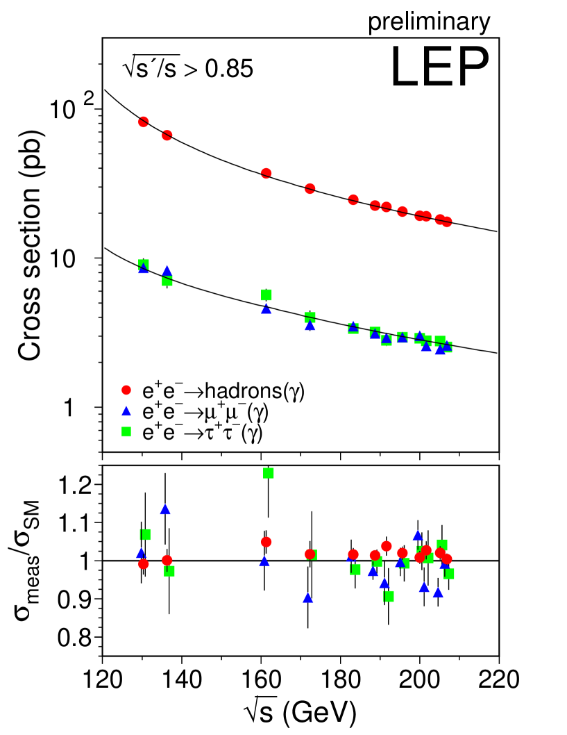
Figure 8.2: Preliminary combined LEP results on the cross-sections for $\mathrm{q\overline{q}}$, $\mu^{+}\mu^{-}$ and $\tau^{+}\tau^{-}$ final states, as a function of centre-of-mass energy. The expectations of the SM, computed with ZFITTER [80], are shown as curves. The lower plot shows the ratio of the data divided by the SM.

Figures 8.2 and 8.3 show the LEP averaged cross-sections and asymmetries, respectively, as a function of the centre-of-mass energy, together with the SM predictions. There is good agreement between the SM expectations and the measurements of the individual experiments and the combined averages. The cross-sections for hadronic final states at most of the energy points are somewhat above the SM expectations. Taking into account the correlations between the data points and also taking into account the theoretical error on the SM predictions, the ratio of the measured cross-sections to the SM expectations, averaged over all energies, is approximately a $1.7$ standard deviation excess. It is concluded that there is no significant evidence in the results of the combinations for physics beyond the SM in the process $\mathrm{e}^{+}\mathrm{e}^{-}\rightarrow\mathrm{f\overline{f}}$.

$\sqrt{s}$ Average (${\mathrm{Ge\kern-1.00006ptV}}$) Quantity value SM $\Delta$ 130 $\sigma(q\overline{q})$ 82.1$\pm$ 2.2 82.8 -0.3 130 $\sigma(\mu^{+}\mu^{-})$ 8.62$\pm$ 0.68 8.44 -0.33 130 $\sigma(\tau^{+}\tau^{-})$ 9.02$\pm$ 0.93 8.44 -0.11 130 $\mathrm{A_{FB}}(\mu^{+}\mu^{-})$ 0.694$\pm$ 0.060 0.705 0.012 130 $\mathrm{A_{FB}}(\tau^{+}\tau^{-})$ 0.663$\pm$ 0.076 0.704 0.012 136 $\sigma(q\overline{q})$ 66.7$\pm$ 2.0 66.6 -0.2 136 $\sigma(\mu^{+}\mu^{-})$ 8.27$\pm$ 0.67 7.28 -0.28 136 $\sigma(\tau^{+}\tau^{-})$ 7.078$\pm$ 0.820 7.279 -0.091 136 $\mathrm{A_{FB}}(\mu^{+}\mu^{-})$ 0.708$\pm$ 0.060 0.684 0.013 136 $\mathrm{A_{FB}}(\tau^{+}\tau^{-})$ 0.753$\pm$ 0.088 0.683 0.014 161 $\sigma(q\overline{q})$ 37.0$\pm$ 1.1 35.2 -0.1 161 $\sigma(\mu^{+}\mu^{-})$ 4.61$\pm$ 0.36 4.61 -0.18 161 $\sigma(\tau^{+}\tau^{-})$ 5.67$\pm$ 0.54 4.61 -0.06 161 $\mathrm{A_{FB}}(\mu^{+}\mu^{-})$ 0.538$\pm$ 0.067 0.609 0.017 161 $\mathrm{A_{FB}}(\tau^{+}\tau^{-})$ 0.646$\pm$ 0.077 0.609 0.016 172 $\sigma(q\overline{q})$ 29.23$\pm$ 0.99 28.74 -0.12 172 $\sigma(\mu^{+}\mu^{-})$ 3.57$\pm$ 0.32 3.95 -0.16 172 $\sigma(\tau^{+}\tau^{-})$ 4.01$\pm$ 0.45 3.95 -0.05 172 $\mathrm{A_{FB}}(\mu^{+}\mu^{-})$ 0.675$\pm$ 0.077 0.591 0.018 172 $\mathrm{A_{FB}}(\tau^{+}\tau^{-})$ 0.342$\pm$ 0.094 0.591 0.017 183 $\sigma(q\overline{q})$ 24.59$\pm$ 0.42 24.20 -0.11 183 $\sigma(\mu^{+}\mu^{-})$ 3.49$\pm$ 0.15 3.45 -0.14 183 $\sigma(\tau^{+}\tau^{-})$ 3.37$\pm$ 0.17 3.45 -0.05 183 $\mathrm{A_{FB}}(\mu^{+}\mu^{-})$ 0.559$\pm$ 0.035 0.576 0.018 183 $\mathrm{A_{FB}}(\tau^{+}\tau^{-})$ 0.608$\pm$ 0.045 0.576 0.018 189 $\sigma(q\overline{q})$ 22.47$\pm$ 0.24 22.156 -0.101 189 $\sigma(\mu^{+}\mu^{-})$ 3.123$\pm$ 0.076 3.207 -0.131 189 $\sigma(\tau^{+}\tau^{-})$ 3.20$\pm$ 0.10 3.20 -0.048 189 $\mathrm{A_{FB}}(\mu^{+}\mu^{-})$ 0.569$\pm$ 0.021 0.569 0.019 189 $\mathrm{A_{FB}}(\tau^{+}\tau^{-})$ 0.596$\pm$ 0.026 0.569 0.018

$\sqrt{s}$ Average (${\mathrm{Ge\kern-1.00006ptV}}$) Quantity value SM $\Delta$ 192 $\sigma(q\overline{q})$ 22.05$\pm$ 0.53 21.24 -0.10 192 $\sigma(\mu^{+}\mu^{-})$ 2.92$\pm$ 0.18 3.10 -0.13 192 $\sigma(\tau^{+}\tau^{-})$ 2.81$\pm$ 0.23 3.10 -0.05 192 $\mathrm{A_{FB}}(\mu^{+}\mu^{-})$ 0.553$\pm$ 0.051 0.566 0.019 192 $\mathrm{A_{FB}}(\tau^{+}\tau^{-})$ 0.615$\pm$ 0.069 0.566 0.019 196 $\sigma(q\overline{q})$ 20.53$\pm$ 0.34 20.13 -0.09 196 $\sigma(\mu^{+}\mu^{-})$ 2.94$\pm$ 0.11 2.96 -0.12 196 $\sigma(\tau^{+}\tau^{-})$ 2.94$\pm$ 0.14 2.96 -0.05 196 $\mathrm{A_{FB}}(\mu^{+}\mu^{-})$ 0.581$\pm$ 0.031 0.562 0.019 196 $\mathrm{A_{FB}}(\tau^{+}\tau^{-})$ 0.505$\pm$ 0.044 0.562 0.019 200 $\sigma(q\overline{q})$ 19.25$\pm$ 0.32 19.09 -0.09 200 $\sigma(\mu^{+}\mu^{-})$ 3.02$\pm$ 0.11 2.83 -0.12 200 $\sigma(\tau^{+}\tau^{-})$ 2.90$\pm$ 0.14 2.83 -0.04 200 $\mathrm{A_{FB}}(\mu^{+}\mu^{-})$ 0.524$\pm$ 0.031 0.558 0.019 200 $\mathrm{A_{FB}}(\tau^{+}\tau^{-})$ 0.539$\pm$ 0.042 0.558 0.019 202 $\sigma(q\overline{q})$ 19.07$\pm$ 0.44 18.57 -0.09 202 $\sigma(\mu^{+}\mu^{-})$ 2.58$\pm$ 0.14 2.77 -0.12 202 $\sigma(\tau^{+}\tau^{-})$ 2.79$\pm$ 0.20 2.77 -0.04 202 $\mathrm{A_{FB}}(\mu^{+}\mu^{-})$ 0.547$\pm$ 0.047 0.556 0.020 202 $\mathrm{A_{FB}}(\tau^{+}\tau^{-})$ 0.589$\pm$ 0.059 0.556 0.019 205 $\sigma(q\overline{q})$ 18.17$\pm$ 0.31 17.81 -0.09 205 $\sigma(\mu^{+}\mu^{-})$ 2.45$\pm$ 0.10 2.67 -0.11 205 $\sigma(\tau^{+}\tau^{-})$ 2.78$\pm$ 0.14 2.67 -0.042 205 $\mathrm{A_{FB}}(\mu^{+}\mu^{-})$ 0.565$\pm$ 0.035 0.553 0.020 205 $\mathrm{A_{FB}}(\tau^{+}\tau^{-})$ 0.571$\pm$ 0.042 0.553 0.019 207 $\sigma(q\overline{q})$ 17.49$\pm$ 0.26 17.42 -0.08 207 $\sigma(\mu^{+}\mu^{-})$ 2.595$\pm$ 0.088 2.623 -0.111 207 $\sigma(\tau^{+}\tau^{-})$ 2.53$\pm$ 0.11 2.62 -0.04 207 $\mathrm{A_{FB}}(\mu^{+}\mu^{-})$ 0.542$\pm$ 0.027 0.552 0.020 207 $\mathrm{A_{FB}}(\tau^{+}\tau^{-})$ 0.564$\pm$ 0.037 0.551 0.019

Table 8.2: Preliminary combined LEP results for $\mathrm{e}^{+}\mathrm{e}^{-}\rightarrow\mathrm{f\overline{f}}$, with cross section quoted in units of picobarn. All the results correspond to the first signal definition. The Standard Model predictions are from ZFITTER [80]. The difference, $\Delta$, in the predictions of ZFITTER for second definition relative to the first are given in the final column. The quoted uncertainties do not include the theoretical uncertainties on the corrections discussed in the text.

$\begin{array}[b]{c}\sqrt{s}\\ ({\mathrm{Ge\kern-1.00006ptV}})\end{array}$	130	136	161	172	183	189	192	196	200	202	205	207
130	1.000	0.071	0.080	0.072	0.114	0.146	0.077	0.105	0.120	0.086	0.117	0.138
136	0.071	1.000	0.075	0.067	0.106	0.135	0.071	0.097	0.110	0.079	0.109	0.128
161	0.080	0.075	1.000	0.077	0.120	0.153	0.080	0.110	0.125	0.090	0.124	0.145
172	0.072	0.067	0.077	1.000	0.108	0.137	0.072	0.099	0.112	0.081	0.111	0.130
183	0.114	0.106	0.120	0.108	1.000	0.223	0.117	0.158	0.182	0.129	0.176	0.208
189	0.146	0.135	0.153	0.137	0.223	1.000	0.151	0.206	0.235	0.168	0.226	0.268
192	0.077	0.071	0.080	0.072	0.117	0.151	1.000	0.109	0.126	0.090	0.118	0.138
196	0.105	0.097	0.110	0.099	0.158	0.206	0.109	1.000	0.169	0.122	0.162	0.190
200	0.120	0.110	0.125	0.112	0.182	0.235	0.126	0.169	1.000	0.140	0.184	0.215
202	0.086	0.079	0.090	0.081	0.129	0.168	0.090	0.122	0.140	1.000	0.132	0.153
205	0.117	0.109	0.124	0.111	0.176	0.226	0.118	0.162	0.184	0.132	1.000	0.213
207	0.138	0.128	0.145	0.130	0.208	0.268	0.138	0.190	0.215	0.153	0.213	1.000

Table 8.3: The correlation coefficients between averaged hadronic cross-sections at different energies.

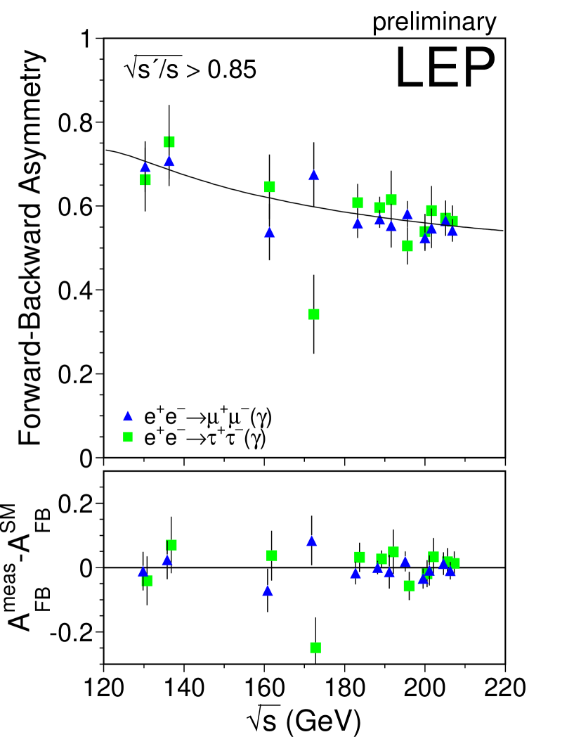
Figure 8.3: Preliminary combined LEP results on the forward-backward asymmetry for $\mu^{+}\mu^{-}$ and $\tau^{+}\tau^{-}$ final states as a function of centre-of-mass energy. The expectations of the SM computed with ZFITTER [80], are shown as curves. The lower plot shows differences between the data and the SM.

8.3 Averages for Differential Cross-sections

8.3.1 $\mathrm{e}^{+}\mathrm{e}^{-}$ final state

The LEP experiments have measured the differential cross-section, $\frac{{\mathrm{d}}\sigma}{{\mathrm{d}}\cos\theta}$, for the $\mathrm{e}^{+}\mathrm{e}^{-}\rightarrow\mathrm{e}^{+}\mathrm{e}^{-}$ channel.A preliminary combination of these results is made by performing a $\chi^{2}$ fit to the measured differential cross-sections, using the statistical errors as given by the experiments. In contrast to the muon and tau channels (Section 8.3.2) the higher statistics makes the use of expected statistical errors unnecessary. The combination includes data from 189 ${\mathrm{Ge\kern-1.00006ptV}}$ to 207 ${\mathrm{Ge\kern-1.00006ptV}}$ from all experiments but DELPHI. The data used in the combination are summarised in Table 8.4.

Each experiment’s data are binned according to an agreed common definition, which takes into account the large forward peak of Bhabha scattering:

• 10 bins for $\cos\theta$ between $0.0$ and $0.90$ and

• 5 bins for $\cos\theta$ between $-0.90$ and $0.0$

at each energy. The scattering angle, $\theta$, is the angle of the negative lepton with respect to the incoming electron direction in the lab coordinate system. The outer acceptances of the most forward and most backward bins for which the experiments present their data are different. The ranges in $\cos\theta$ of the individual experiments and the average are given in Table 8.5. Except for the binning, each experiment uses their own signal definition, for example different experiments have different acollinearity cuts to select events. The signal definition used for the LEP average corresponds to an acollinearity cut of $\rm 10^{\circ}$. The experimental measurements are corrected to the common signal definition following the procedure described in Section 8.2. The theoretical predictions are taken from the Monte Carlo event generator BHWIDE [82].

Correlated systematic errors between different experiments, energies and bins at the same energy, arising from uncertainties on the overall normalisation, and from migration of events between forward and backward bins with the same absolute value of $\cos\theta$ due to uncertainties in the corrections for charge confusion, were considered in the averaging procedure.

An average for all energies between 189–207 ${\mathrm{Ge\kern-1.00006ptV}}$ is performed. The results of the averages are shown in Figure 8.4. The $\chi^{2}$ per degree of freedom for the average is $190.8/189$.

The correlations between bins in the average are well below $5\%$ of the total error on the averages in each bin for most of the cases, and exceed $10\%$ for the most forward bin for the energy points with the highest accumulated statistics. The agreement between the averaged data and the predictions from the Monte Carlo generator BHWIDE is good.

8.3.2 $\mu^{+}\mu^{-}$and $\tau^{+}\tau^{-}$ final states

The LEP experiments have measured the differential cross-section, $\frac{{\mathrm{d}}\sigma}{{\mathrm{d}}\cos\theta}$, for the $\mathrm{e}^{+}\mathrm{e}^{-}\rightarrow\mu^{+}\mu^{-}$ and $\mathrm{e}^{+}\mathrm{e}^{-}\rightarrow\tau^{+}\tau^{-}$ channels for samples of events with high effective centre-of-mass energy, $\sqrt{s^{\prime}/s}>0.85$. A preliminary combination of these results is made using the BLUE technique. The statistical error associated with each measurement is taken as the expected statistical error on the differential cross-section, computed from the expected number of events in each bin for each experiment. Using a Monte Carlo simulation it has been shown that this method provides a good approximation to the exact likelihood method based on Poisson statistics [83].

The combination includes data from 183 ${\mathrm{Ge\kern-1.00006ptV}}$ to 207 ${\mathrm{Ge\kern-1.00006ptV}}$, but not all experiments provided data at all energies. The data used in the combination are summarised in Table 8.6.

Each experiment’s data are binned in 10 bins of $\cos\theta$ at each energy, using their own signal definition. The scattering angle, $\theta$, is the angle of the negative lepton with respect to the incoming electron direction in the lab coordinate system. The outer acceptances of the most forward and most backward bins for which the four experiments present their data are different. This was accounted for as part of the correction to a common signal definition. The ranges in $\cos\theta$ for the measurements of the individual experiments and the average are given in Table 8.7. The signal definition used corresponded to the first definition given in Section 8.2.

Correlated systematic errors between different experiments, channels and energies, arising from uncertainties on the overall normalisation are considered in the averaging procedure. All data from all energies are combined in a single fit to obtain averages at each centre-of-mass energy yielding the full covariance matrix between the different measurements at all energies.

The results of the averages are shown in Figures 8.5 and 8.6. The correlations between bins in the average are less that $2\%$ of the total error on the averages in each bin. Overall the agreement between the averaged data and the predictions is reasonable, with a $\chi^{2}$ of $200$ for $160$ degrees of freedom. At 202 ${\mathrm{Ge\kern-1.00006ptV}}$ the measured differential cross-sections in the most backward bins, $-1.00<\cos\theta<0.8$, for both muon and tau final states are above the predictions. The data at 202 ${\mathrm{Ge\kern-1.00006ptV}}$ suffer from rather low delivered luminosity, with less than 4 events expected in each experiment in each channel in this backward $\cos\theta$ bin. The agreement between the data and the predictions in the same $\cos\theta$ bin is more consistent at higher energies.

	$\mathrm{e}^{+}\mathrm{e}^{-}\rightarrow\mathrm{e}^{+}\mathrm{e}^{-}$
$\sqrt{s}$(${\mathrm{Ge\kern-1.00006ptV}}$)	A	D	L	O
189	P	-	P	F
192–202	P	-	P	P
205–207	P	-	P	P

Table 8.4: Differential cross-section data provided by the LEP collaborations (ALEPH, DELPHI, L3 and OPAL) for $\mathrm{e}^{+}\mathrm{e}^{-}\rightarrow\mathrm{e}^{+}\mathrm{e}^{-}$. Data indicated with F are final, published data. Data marked with P are preliminary. Data marked with a - were not available for combination.

Experiment	$\cos\theta_{min}$	$\cos\theta_{max}$
ALEPH ($\sqrt{s^{\prime}/s}>0.85$)	$-0.90$	$0.90$
L3 (acol. $<\ 25^{\circ}$)	$-0.72$	$0.72$
OPAL (acol. $<\ 10^{\circ}$)	$-0.90$	$0.90$
Average (acol. $<\ 10^{\circ}$)	$-0.90$	$0.90$

Table 8.5: The acceptances for which experimental data are presented for the $\mathrm{e}^{+}\mathrm{e}^{-}\rightarrow\mathrm{e}^{+}\mathrm{e}^{-}$ channel and the acceptance for the LEP average.

	$\mathrm{e}^{+}\mathrm{e}^{-}\rightarrow\mu^{+}\mu^{-}$				$\mathrm{e}^{+}\mathrm{e}^{-}\rightarrow\tau^{+}\tau^{-}$
$\sqrt{s}$(${\mathrm{Ge\kern-1.00006ptV}}$)	A	D	L	O	A	D	L	O
183	-	F	-	F	-	F	-	F
189	P	F	F	F	P	F	F	F
192–202	P	P	P	P	P	P	-	P
205–207	P	P	P	P	P	P	-	P

Table 8.6: Differential cross-section data provided by the LEP collaborations (ALEPH, DELPHI, L3 and OPAL) for $\mathrm{e}^{+}\mathrm{e}^{-}\rightarrow\mu^{+}\mu^{-}$ and $\mathrm{e}^{+}\mathrm{e}^{-}\rightarrow\tau^{+}\tau^{-}$ combination at different centre-of-mass energies. Data indicated with F are final, published data. Data marked with P are preliminary. Data marked with a - were not available for combination.

Experiment	$\cos\theta_{min}$	$\cos\theta_{max}$
ALEPH	$-0.95$	$0.95$
DELPHI ($\mathrm{e}^{+}\mathrm{e}^{-}\rightarrow\mu^{+}\mu^{-}$ 183)	$-0.94$	$0.94$
DELPHI ($\mathrm{e}^{+}\mathrm{e}^{-}\rightarrow\mu^{+}\mu^{-}$ 189–207)	$-0.97$	$0.97$
DELPHI ($\mathrm{e}^{+}\mathrm{e}^{-}\rightarrow\tau^{+}\tau^{-}$)	$-0.96$	$0.96$
L3	$-0.90$	$0.90$
OPAL	$-1.00$	$1.00$
Average	$-1.00$	$1.00$

Table 8.7: The acceptances for which experimental data are presented and the acceptance for the LEP average. For DELPHI the acceptance is shown for the different channels and for the muons for different centre of mass energies. For all other experiments the acceptance is the same for muon and tau-lepton channels and for all energies provided.

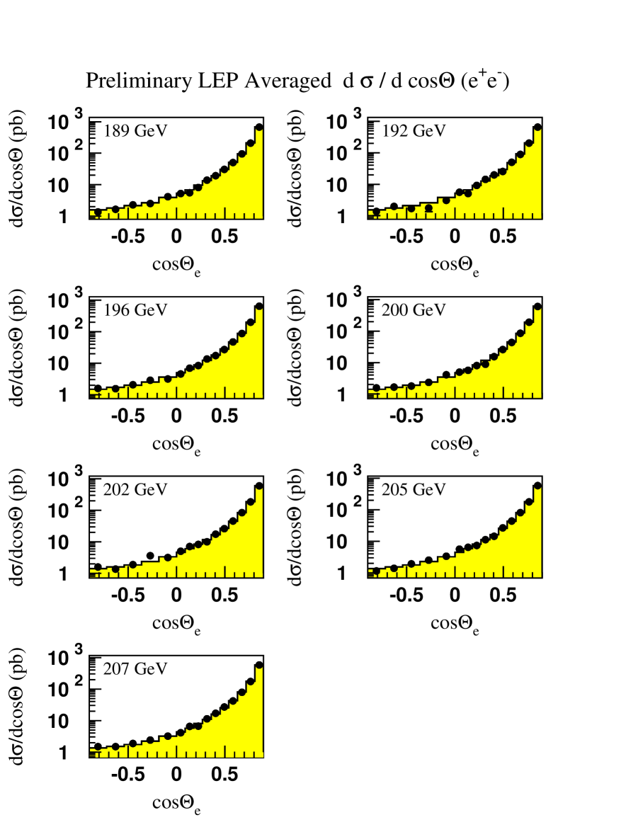
Figure 8.4: LEP averaged differential cross-sections for $\mathrm{e}^{+}\mathrm{e}^{-}\rightarrow\mathrm{e}^{+}\mathrm{e}^{-}$ at energies of 189–207 ${\mathrm{Ge\kern-1.00006ptV}}$. The SM predictions, shown as solid histograms, are computed with BHWIDE [82].

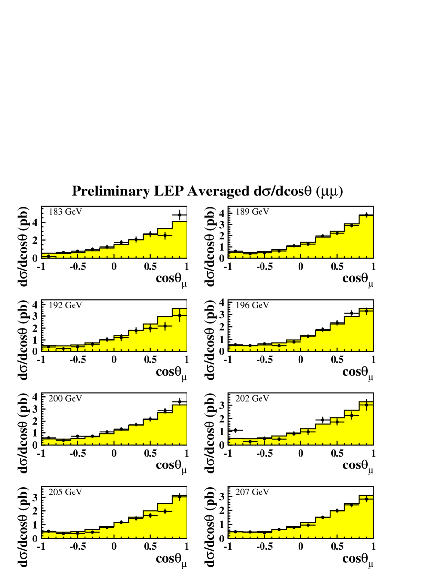
Figure 8.5: LEP averaged differential cross-sections for $\mathrm{e}^{+}\mathrm{e}^{-}\rightarrow\mu^{+}\mu^{-}$ at energies of 183–207 ${\mathrm{Ge\kern-1.00006ptV}}$. The SM predictions, shown as solid histograms, are computed with ZFITTER [80].

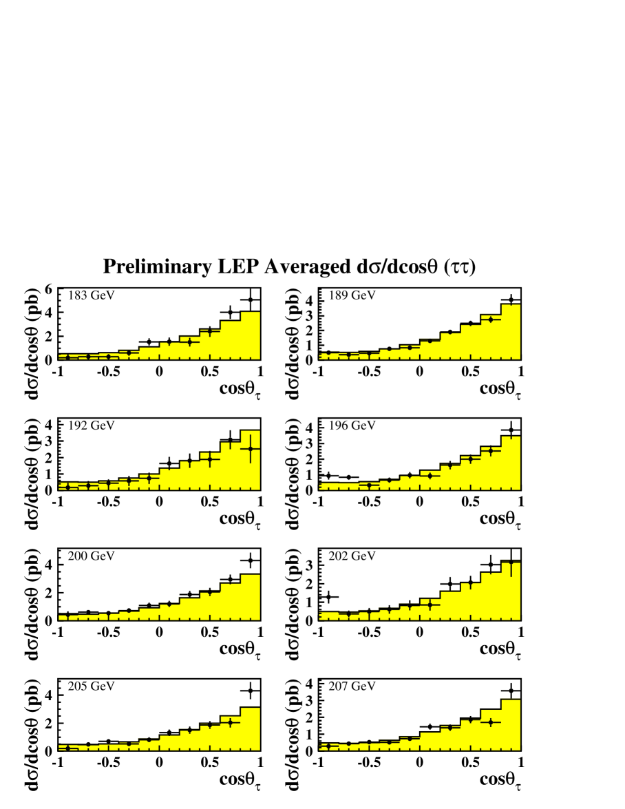
Figure 8.6: LEP averaged differential cross-sections for $\mathrm{e}^{+}\mathrm{e}^{-}\rightarrow\tau^{+}\tau^{-}$ at energies of 183–207 ${\mathrm{Ge\kern-1.00006ptV}}$. The SM predictions, shown as solid histograms, are computed with ZFITTER [80].

8.4 Averages for Heavy Flavour Measurements

This section presents a preliminary combination of both published [84] and preliminary [85] measurements of the ratios cross section ratios $R_{\mathrm{q}}$ defined as ${\mathrm{\frac{\sigma_{q\overline{q}}}{\sigma_{had}}}}$ for b and c production, $R_{\mathrm{b}}$ and $R_{\mathrm{c}}$, and the forward-backward asymmetries, $A_{\mathrm{FB}}^{\mathrm{b\overline{b}}}$ and $A_{\mathrm{FB}}^{\mathrm{c\overline{c}}}$, from the LEP collaborations at centre-of-mass energies in the range of 130 ${\mathrm{Ge\kern-1.00006ptV}}$ to 207 ${\mathrm{Ge\kern-1.00006ptV}}$. Table 8.8 summarises all the inputs that have been combined so far.

A common signal definition is defined for all the measurements, requiring:

• an effective centre-of-mass energy $\sqrt{s^{\prime}}>0.85\sqrt{s}$

• no subtraction of ISR and FSR photon interference contribution and

• extrapolation to full angular acceptance.

Systematic errors are divided into three categories: uncorrelated errors, errors correlated between the measurements of each experiment, and errors common to all experiments.

Due to the fact that $R_{\mathrm{c}}$ measurements are only provided by a single experiment and are strongly correlated with $R_{\mathrm{b}}$ measurements, it was decided to fit the b sector and c sector separately, the other flavour’s measurements being fixed to their Standard Model predictions. In addition, these fitted values are used to set limits upon physics beyond the Standard Model, such as contact term interactions, in which only one quark flavour is assumed to be effected by the new physics during each fit, therefore this averaging method is consistent with the interpretations.

Full details concerning the combination procedure can be found in [86].

The results of the combination are presented in Table 8.9 and Table 8.10 and in Figures 8.7 and 8.8. The results for both b and c sector are in agreement with the Standard Model predictions of ZFITTER. The averaged discrepancies with respect to the Standard Model predictions is -2.08 $\sigma$ for $R_{\mathrm{b}}$, +0.30 $\sigma$ for $R_{\mathrm{c}}$, -1.56 $\sigma$ for $A_{\mathrm{FB}}^{\mathrm{b\overline{b}}}$ and -0.24 $\sigma$ for $A_{\mathrm{FB}}^{\mathrm{c\overline{c}}}$. A list of the error contributions from the combination at 189 ${\mathrm{Ge\kern-1.00006ptV}}$ is shown in Table 8.11.

$\sqrt{s}$ (${\mathrm{Ge\kern-1.00006ptV}}$)	$R_{\mathrm{b}}$				$R_{\mathrm{c}}$				$A_{\mathrm{FB}}^{\mathrm{b\overline{b}}}$				$A_{\mathrm{FB}}^{\mathrm{c\overline{c}}}$
	A	D	L	O	A	D	L	O	A	D	L	O	A	D	L	O
133	F	F	F	F	-	-	-	-	-	F	-	F	-	F	-	F
167	F	F	F	F	-	-	-	-	-	F	-	F	-	F	-	F
183	F	P	F	F	F	-	-	-	F	-	-	F	P	-	-	F
189	P	P	F	F	P	-	-	-	P	P	F	F	P	-	-	F
192 to 202	P	P	P	-	P*	-	-	-	P	P	-	-	-	-	-	-
205 and 207	-	P	P	-	P	-	-	-	P	P	-	-	-	-	-	-

Table 8.8: Data provided by the ALEPH, DELPHI, L3, OPAL collaborations for combination at different centre-of-mass energies. Data indicated with F are final, published data. Data marked with P are preliminary and for data marked with P*, not all energies are supplied. Data marked with a - were not supplied for combination.

$\sqrt{s}$ (${\mathrm{Ge\kern-1.00006ptV}}$)	$R_{\mathrm{b}}$	$A_{\mathrm{FB}}^{\mathrm{b\overline{b}}}$
133	0.1822 $\pm$ 0.0132	0.367 $\pm$ 0.251
	(0.1867)	(0.504)
167	0.1494 $\pm$ 0.0127	0.624 $\pm$ 0.254
	(0.1727)	(0.572)
183	0.1646 $\pm$ 0.0094	0.515 $\pm$ 0.149
	(0.1692)	(0.588)
189	0.1565 $\pm$ 0.0061	0.529 $\pm$ 0.089
	(0.1681)	(0.593)
192	0.1551 $\pm$ 0.0149	0.424 $\pm$ 0.267
	(0.1676)	(0.595)
196	0.1556 $\pm$ 0.0097	0.535 $\pm$ 0.151
	(0.1670)	(0.598)
200	0.1683 $\pm$ 0.0099	0.596 $\pm$ 0.149
	(0.1664)	(0.600)
202	0.1646 $\pm$ 0.0144	0.607 $\pm$ 0.241
	(0.1661)	(0.601)
205	0.1606 $\pm$ 0.0126	0.715 $\pm$ 0.214
	(0.1657)	(0.603)
207	0.1694 $\pm$ 0.0107	0.175 $\pm$ 0.156
	(0.1654)	(0.604)

Table 8.9: Combined results on $R_{\mathrm{b}}$ and $A_{\mathrm{FB}}^{\mathrm{b\overline{b}}}$. Quoted errors represent the statistical and systematic errors added in quadrature. For comparison, the Standard Model predictions computed with ZFITTER [87] are given in parentheses.

$\sqrt{s}$ (${\mathrm{Ge\kern-1.00006ptV}}$)	$R_{\mathrm{c}}$	$A_{\mathrm{FB}}^{\mathrm{c\overline{c}}}$
133	-	0.630 $\pm$ 0.313
		(0.684)
167	-	0.980 $\pm$ 0.343
		(0.677)
183	0.2628 $\pm$ 0.0397	0.717 $\pm$ 0.201
	(0.2472)	(0.663)
189	0.2298 $\pm$ 0.0213	0.542 $\pm$ 0.143
	(0.2490)	(0.656)
196	0.2734 $\pm$ 0.0387	-
	(0.2508)
200	0.2535 $\pm$ 0.0360	-
	(0.2518)
205	0.2816 $\pm$ 0.0394	-
	(0.2530)
207	0.2890 $\pm$ 0.0350	-
	(0.2533)

Table 8.10: Combined results on $R_{\mathrm{c}}$ and $A_{\mathrm{FB}}^{\mathrm{c\overline{c}}}$. Quoted errors represent the statistical and systematic errors added in quadrature. For comparison, the Standard Model predictions computed with ZFITTER [87] are given in parentheses.

Error list	$R_{\mathrm{b}}$ (189 ${\mathrm{Ge\kern-1.00006ptV}}$)	$A_{\mathrm{FB}}^{\mathrm{b\overline{b}}}$ (189 ${\mathrm{Ge\kern-1.00006ptV}}$)	$R_{\mathrm{c}}$ (189 ${\mathrm{Ge\kern-1.00006ptV}}$)	$A_{\mathrm{FB}}^{\mathrm{c\overline{c}}}$ (189 ${\mathrm{Ge\kern-1.00006ptV}}$)
statistics	0.0057	0.084	0.0169	0.119
internal syst	0.0020	0.025	0.0109	0.042
common syst	0.0007	0.011	0.0072	0.069
total syst	0.0021	0.027	0.0130	0.081
total error	0.0061	0.089	0.0213	0.143

Table 8.11: Error breakdown at 189 ${\mathrm{Ge\kern-1.00006ptV}}$.

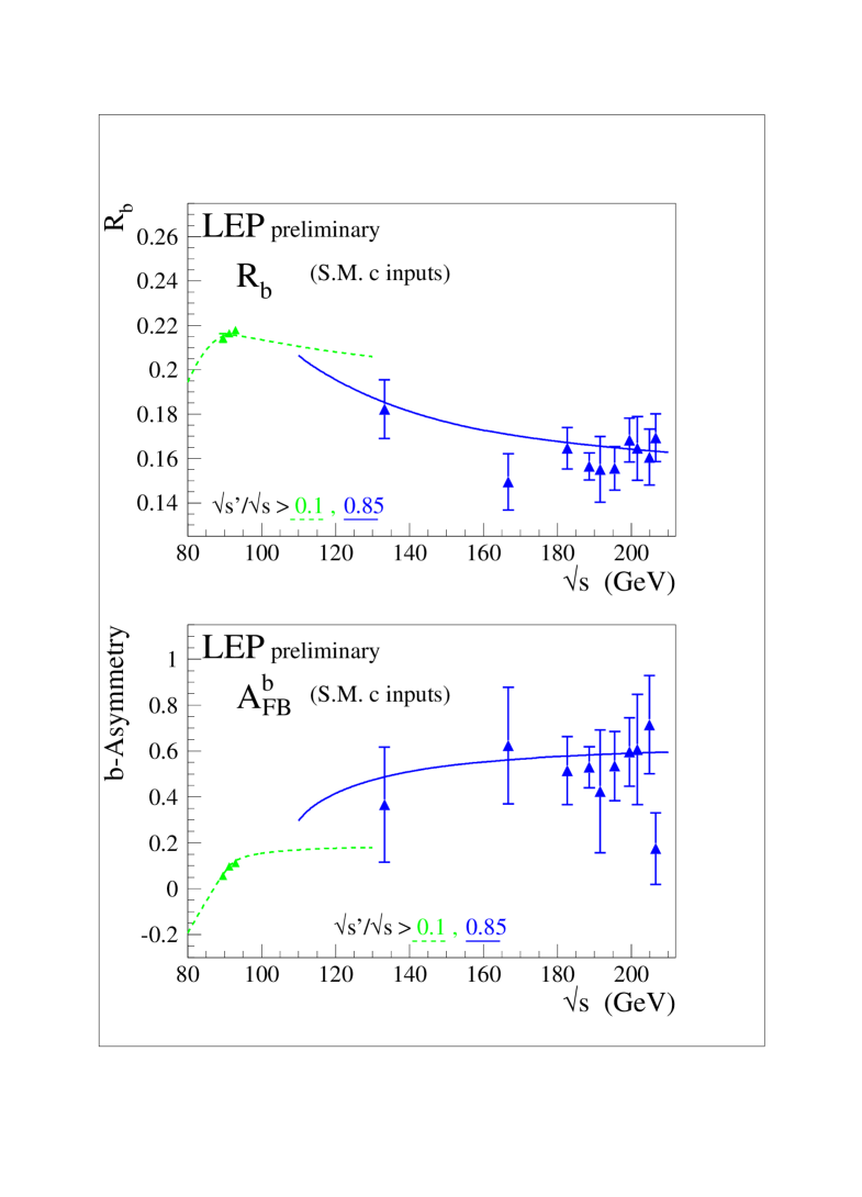
Figure 8.7: Preliminary combined LEP measurements of $R_{\mathrm{b}}$ and $A_{\mathrm{FB}}^{\mathrm{b\overline{b}}}$. Solid lines represent the Standard Model prediction for the high $\sqrt{s^{\prime}}$ selection used at LEP-II and dotted lines the inclusive prediction used at LEP-I. Both are computed with ZFITTER[87]. The LEP-I measurements have been taken from [88].

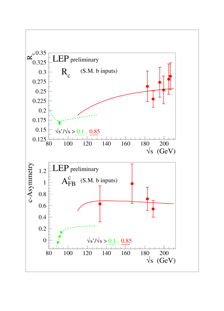
Figure 8.8: Preliminary combined LEP measurements of $R_{\mathrm{c}}$ and $A_{\mathrm{FB}}^{\mathrm{c\overline{c}}}$. Solid lines represent the Standard Model prediction for the high $\sqrt{s^{\prime}}$ selection used at LEP-II and dotted lines the inclusive prediction used at LEP-I. Both are computed with ZFITTER [87]. The LEP-I measurements have been taken from [88].

8.5 Interpretation

The combined measurements presented above are interpreted in a variety of models. The cross-section and asymmetry results are used to place limits on contact interactions between leptons and quarks and, using the results on heavy flavour production, on contact interaction between electrons and $b$ and $c$ quarks specifically. Limits on the mass of a possible additional heavy neutral boson, $\mathrm{Z^{\prime}}$, are obtained for a variety of models. Using the combined differential cross-sections for $\mathrm{e}^{+}\mathrm{e}^{-}$ final states, limits on contact interactions in the $\mathrm{e}^{+}\mathrm{e}^{-}\rightarrow\mathrm{e}^{+}\mathrm{e}^{-}$ channel and limits on the scale of gravity in models with large extra-dimensions are presented. Limits are also derived on the masses of leptoquarks - assuming a coupling of electromagnetic strength. In all cases the Born level predictions for the physics beyond the Standard Model have been corrected to take into account QED radiation.

8.5.1 Contact Interactions

The averages of cross-sections and forward-backward asymmetries for muon-pair and tau-lepton pair and the cross-sections for $\mathrm{q\overline{q}}$ final states are used to search for contact interactions between fermions.

Following [89], contact interactions are parameterised by an effective Lagrangian, $\cal{L}_{\mathrm{eff}}$, which is added to the Standard Model Lagrangian and has the form:

$$\mbox{$\cal{L}$}_{\mathrm{eff}}=\frac{g^{2}}{(1+\delta)\Lambda^{2}}\sum_{i,j=L,R}\eta_{ij}\overline{e}_{i}\gamma_{\mu}e_{i}\overline{f}_{j}\gamma^{\mu}f_{j},$$ (8.2)

where $g^{2}/{4\pi}$ is taken to be 1 by convention, $\delta=1(0)$ for $f=e\leavevmode\nobreak\ (f\neq e)$, $\eta_{ij}=\pm 1$ or $\mathrm{𝟎}$ for different interaction types, $\Lambda$ is the scale of the contact interactions, $e_{i}$ and $f_{j}$ are left or right-handed spinors. By assuming different helicity coupling between the initial state and final state currents, a set of different models can be defined from this Lagrangian [90], with either constructive ($+$) or destructive ($-$) interference between the Standard Model process and the contact interactions. The models and corresponding choices of $\eta_{ij}$ are given in Table 8.12. The models LL^±, RR^±, VV^±, AA^±, LR^±, RL^±, V0^±, A0^± are considered here since these models lead to large deviations in $\mathrm{e}^{+}\mathrm{e}^{-}\rightarrow\mathrm{f\overline{f}}$ at LEP II. The corresponding energies scales for the models with constructive or destructive interference are denoted by $\Lambda^{+}$ and $\Lambda^{-}$ respectively.

For leptonic final states 4 different fits are made

• individual fits to contact interactions in $\mathrm{e}^{+}\mathrm{e}^{-}\rightarrow\mu^{+}\mu^{-}$ and $\mathrm{e}^{+}\mathrm{e}^{-}\rightarrow\tau^{+}\tau^{-}$ using the measured cross-sections and asymmetries,

• fits to $\mathrm{e}^{+}\mathrm{e}^{-}\rightarrow\ell^{+}\ell^{-}$ (simultaneous fits to $\mathrm{e}^{+}\mathrm{e}^{-}\rightarrow\mu^{+}\mu^{-}$ and $\mathrm{e}^{+}\mathrm{e}^{-}\rightarrow\tau^{+}\tau^{-}$) again using the measured cross-sections and asymmetries,

• fits to $\mathrm{e}^{+}\mathrm{e}^{-}\rightarrow\mathrm{e}^{+}\mathrm{e}^{-}$, using the measured differential cross-sections.

For the inclusive hadronic final states three different model assumptions are used to fit the total hadronic cross-section

• the contact interactions affect only one quark flavour of up-type using the measured hadronic cross-sections,

• the contact interactions affect only one quark flavour of down-type using the measured hadronic cross-sections,

• the contact interactions contribute to all quark final states with the same strength.

Limits on contact interactions between electrons and $b$ and $c$ quarks are obtained using all the heavy flavour LEP-II combined results from 133 ${\mathrm{Ge\kern-1.00006ptV}}$ to 207 ${\mathrm{Ge\kern-1.00006ptV}}$ given in Tables 8.9 and 8.10. For the purpose of fitting contact interaction models to the data, $R_{\mathrm{b}}$ and $R_{\mathrm{c}}$ are converted to cross-sections $\sigma_{\mathrm{b\overline{b}}}$ and $\sigma_{\mathrm{c\overline{c}}}$ using the averaged ${\mathrm{q\overline{q}}}$ cross-section of section 8.2 corresponding to the second signal definition. In the calculation of errors, the correlations between $R_{\mathrm{b}}$, $R_{\mathrm{c}}$ and $\sigma_{\mathrm{q\overline{q}}}$ are assumed to be negligible. These results are of particular interest since they are inaccessible to ${\mathrm{p\bar{p}}}$ or ep colliders.

For the purpose of fitting contact interaction models to the data, the parameter $\epsilon=1/\Lambda^{2}$ is used, with $\epsilon=0$ in the limit that there are no contact interactions. This parameter is allowed to take both positive and negative values in the fits. Theoretical uncertainties on the Standard Model predictions are taken from [79].

The values of $\epsilon$ extracted for each model are all compatible with the Standard Model expectation $\epsilon=0$, at the two standard deviation level. As expected, the errors on $\epsilon$ are typically a factor of two smaller than those obtained from a single LEP experiment with the same data set. The fitted values of $\epsilon$ are converted into $95\%$ confidence level lower limits on $\Lambda$. The limits are obtained by integrating the likelihood function in $\epsilon$ over the physically allowed values, $\epsilon\geq 0$ for each $\Lambda^{+}$ limit and $\epsilon\leq 0$ for $\Lambda^{-}$ limits.

The fitted values of $\epsilon$ and their 68$\%$ confidence level uncertainties together with the 95$\%$ confidence level lower limit on ${\mathrm{\Lambda}}$ are shown in Table 8.13 for the fits to $\mathrm{e}^{+}\mathrm{e}^{-}\rightarrow\ell^{+}\ell^{-}$ ($\ell\neq e$), $\mathrm{e}^{+}\mathrm{e}^{-}\rightarrow\mathrm{e}^{+}\mathrm{e}^{-}$ , inclusive $\mathrm{e}^{+}\mathrm{e}^{-}\rightarrow\mathrm{q\overline{q}}$, $\mathrm{e}^{+}\mathrm{e}^{-}\rightarrow\mathrm{b\overline{b}}$ and $\mathrm{e}^{+}\mathrm{e}^{-}\rightarrow\mathrm{c\overline{c}}$. Table 8.14 shows only the limits obtained on the scale $\Lambda$ for other fits. The limits are shown graphically in Figure 8.9.

For the VV model with positive interference and assuming electromagnetic coupling strength instead of $g^{2}/{4\pi}=1$, the scale $\Lambda$ obtained in the $\mathrm{e}^{+}\mathrm{e}^{-}\rightarrow\mathrm{e}^{+}\mathrm{e}^{-}$ channel is converted to an upper limit on the electron size:

$$\mathrm{r_{e}<1.4\times 10^{-19}m}$$ (8.3)

Models with stronger couplings will make this upper limit even tighter.

Model	$\eta_{LL}$	$\eta_{RR}$	$\eta_{LR}$	$\eta_{RL}$
LL±	$\pm 1$	0	0	0
RR±	0	$\pm 1$	0	0
VV±	$\pm 1$	$\pm 1$	$\pm 1$	$\pm 1$
AA±	$\pm 1$	$\pm 1$	$\mp 1$	$\mp 1$
LR±	0	0	$\pm 1$	0
RL±	0	0	0	$\pm 1$
V0±	$\pm 1$	$\pm 1$	0	0
A0±	0	0	$\pm 1$	$\pm 1$

Table 8.12: Choices of $\eta_{ij}$ for different contact interaction models

.

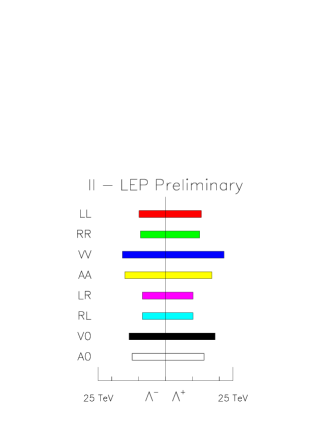
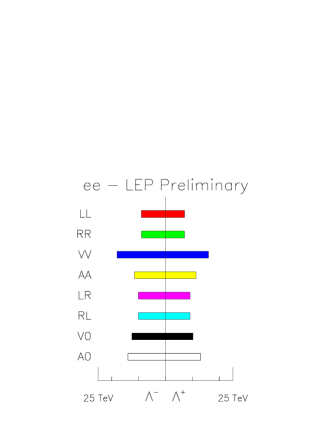
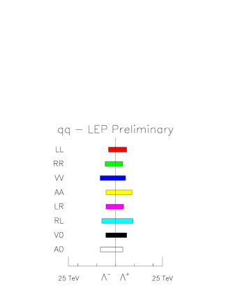
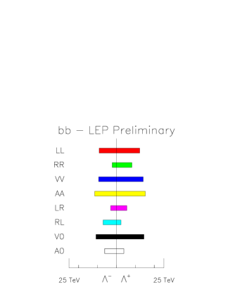
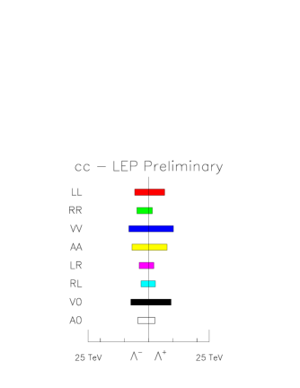
Figure 8.9: The limits on $\Lambda$ for $\mathrm{e}^{+}\mathrm{e}^{-}\rightarrow\ell^{+}\ell^{-}$ assuming universality in the contact interactions between $\mathrm{e}^{+}\mathrm{e}^{-}\rightarrow\ell^{+}\ell^{-}$ ($\ell\neq e$), for $\mathrm{e}^{+}\mathrm{e}^{-}\rightarrow\mathrm{e}^{+}\mathrm{e}^{-}$, for $\mathrm{e}^{+}\mathrm{e}^{-}\rightarrow\mathrm{q\overline{q}}$ assuming equal strength contact interactions for quarks and for $\mathrm{e}^{+}\mathrm{e}^{-}\rightarrow\mathrm{b\overline{b}}$ and $\mathrm{e}^{+}\mathrm{e}^{-}\rightarrow\mathrm{c\overline{c}}$.

$\mathrm{e}^{+}\mathrm{e}^{-}\rightarrow\ell^{+}\ell^{-}$ $\epsilon$ $\Lambda^{-}$ $\Lambda^{+}$ Model (TeV-2) (TeV) (TeV)     LL -0.0044${}^{+0.0035}_{-0.0035}$ 9.8 13.3 RR -0.0049${}^{+0.0039}_{-0.0039}$ 9.3 12.7 VV -0.0016${}^{+0.0013}_{-0.0014}$ 16.0 21.7 AA -0.0013${}^{+0.0017}_{-0.0017}$ 15.1 17.2 LR -0.0036${}^{+0.0052}_{-0.0054}$ 8.6 10.2 RL -0.0036${}^{+0.0052}_{-0.0054}$ 8.6 10.2 V0 -0.0023${}^{+0.0018}_{-0.0018}$ 13.5 18.4 A0 -0.0018${}^{+0.0026}_{-0.0026}$ 12.4 14.3	$\mathrm{e}^{+}\mathrm{e}^{-}\rightarrow\mathrm{e}^{+}\mathrm{e}^{-}$ $\epsilon$ $\Lambda^{-}$ $\Lambda^{+}$ Model (TeV-2) (TeV) (TeV)     LL  0.0049${}^{+0.0084}_{-0.0084}$ 9.0 7.1 RR  0.0056${}^{+0.0082}_{-0.0092}$ 8.9 7.0 VV  0.0004${}^{+0.0022}_{-0.0016}$ 18.0 15.9 AA  0.0009${}^{+0.0041}_{-0.0039}$ 11.5 11.3 LR  0.0008${}^{+0.0064}_{-0.0052}$ 10.0 9.1 RL  0.0008${}^{+0.0064}_{-0.0052}$ 10.0 9.1 V0  0.0028${}^{+0.0038}_{-0.0045}$ 12.5 10.2 A0 -0.0008${}^{+0.0028}_{-0.0030}$ 14.0 13.0
$\mathrm{e}^{+}\mathrm{e}^{-}\rightarrow\mathrm{q\overline{q}}$ $\epsilon$ $\Lambda^{-}$ $\Lambda^{+}$ Model (TeV-2) (TeV) (TeV)     LL  0.0152${}^{+0.0064}_{-0.0076}$ 3.7 6.0 RR -0.0208${}^{+0.0103}_{-0.0082}$ 5.5 3.9 VV -0.0096${}^{+0.0051}_{-0.0037}$ 8.1 5.3 AA  0.0068${}^{+0.0033}_{-0.0034}$ 5.1 8.8 LR -0.0308${}^{+0.0172}_{-0.0055}$ 5.1 4.3 RL -0.0108${}^{+0.0057}_{-0.0054}$ 7.2 9.3 V0  0.0174${}^{+0.0057}_{-0.0074}$ 5.1 6.0 A0 -0.0092${}^{+0.0049}_{-0.0041}$ 8.0 3.9
$\mathrm{e}^{+}\mathrm{e}^{-}\rightarrow\mathrm{b\overline{b}}$ $\epsilon$ $\Lambda^{-}$ $\Lambda^{+}$ Model (TeV-2) (TeV) (TeV)     LL -0.0038${}^{+0.0044}_{-0.0047}$ 9.1 12.3 RR -0.1729${}^{+0.1584}_{-0.0162}$ 2.2 8.1 VV -0.0040${}^{+0.0039}_{-0.0041}$ 9.4 14.1 AA -0.0022${}^{+0.0029}_{-0.0031}$ 11.5 15.3 LR -0.0620${}^{+0.0692}_{-0.0313}$ 3.1 5.5 RL 0.0180${}^{+0.1442}_{-0.0249}$ 7.0 2.4 V0 -0.0028${}^{+0.0032}_{-0.0033}$ 10.8 14.5 A0 0.0375${}^{+0.0193}_{-0.0379}$ 6.3 3.9	$\mathrm{e}^{+}\mathrm{e}^{-}\rightarrow\mathrm{c\overline{c}}$ $\epsilon$ $\Lambda^{-}$ $\Lambda^{+}$ Model (TeV-2) (TeV) (TeV)     LL -0.0091${}^{+0.0126}_{-0.0126}$ 5.7 6.6 RR 0.3544${}^{+0.0476}_{-0.3746}$ 4.9 1.5 VV -0.0047${}^{+0.0057}_{-0.0060}$ 8.2 10.3 AA -0.0059${}^{+0.0095}_{-0.0090}$ 6.9 7.6 LR 0.1386${}^{+0.0555}_{-0.1649}$ 3.9 2.1 RL 0.0106${}^{+0.0848}_{-0.0757}$ 3.1 2.8 V0 -0.0058${}^{+0.0075}_{-0.0071}$ 7.4 9.2 A0 0.0662${}^{+0.0564}_{-0.0905}$ 4.5 2.7

Table 8.13: The fitted values of $\epsilon$ and the derived 95% confidence level lower limits on the parameter $\Lambda$ of contact interaction derived from fits to lepton-pair cross-sections and asymmetries and from fits to hadronic cross-sections. The limits $\Lambda_{+}$ and $\Lambda_{-}$ given in TeV correspond to the upper and lower signs of the parameters $\eta_{ij}$ in Table 8.12. For $\ell^{+}\ell^{-}$ ($\ell\neq e$) the couplings to $\mu^{+}\mu^{-}$ and $\tau^{+}\tau^{-}$ are a assumed to be universal and for inclusive $\mathrm{q\overline{q}}$ final states all quarks are assumed to experience contact interactions with the same strength.

leptons $\mu^{+}\mu^{-}$ $\tau^{+}\tau^{-}$ Model   $\Lambda_{-}$   $\Lambda_{+}$   $\Lambda_{-}$   $\Lambda_{+}$     LL 8.5 12.5 9.1 8.6 RR 8.1 11.9 8.7 8.2 VV 14.3 19.7 14.2 14.5 AA 12.7 16.4 14.0 11.3 LR 7.9 8.9 2.2 7.9 RL 7.9 8.9 2.2 7.9 V0 11.7 17.2 12.7 11.8 A0 11.5 12.4 9.8 10.8

hadrons up-type down-type Model   $\Lambda_{-}$   $\Lambda_{+}$   $\Lambda_{-}$   $\Lambda_{+}$     LL 6.7 10.2 10.6 6.0 RR 5.7 8.3 2.2 4.3 VV 9.6 14.3 11.4 7.0 AA 8.0 11.5 13.3 7.7 LR 4.2 2.3 2.7 3.5 RL 3.5 2.8 4.2 2.4 V0 8.7 13.4 12.5 7.1 A0 4.9 2.8 4.2 3.3

Table 8.14: The 95% confidence level lower limits on the parameter $\Lambda$ of contact interaction derived from fits to lepton-pair cross-sections and asymmetries and from fits to hadronic cross-sections. The limits $\Lambda_{+}$ and $\Lambda_{-}$ given in TeV correspond to the upper and lower signs of the parameters $\eta_{ij}$ in Table 8.12. For hadrons the limits for up-type and down-type quarks are derived assuming a single up or down type quark undergoes contact interactions.

8.5.2 Models with $\mathbf{\mathrm{Z^{\prime}}}$ Bosons

The combined hadronic and leptonic cross-sections and the leptonic forward-backward asymmetries are used to fit the data to models including an additional, heavy, neutral boson, $\mathrm{Z^{\prime}}$.

Fits are made to $\mathrm{M}_{\mathrm{Z}^{{}^{\prime}}}$, the mass of a $\mathrm{Z^{\prime}}$ for models resulting from an E₆ GUT and L-R symmetric models [91] and for the Sequential Standard Model (SSM) [92], which proposes the existence of a $\mathrm{Z^{\prime}}$ with exactly the same coupling to fermions as the standard Z. LEP-II data alone does not significantly constrain the mixing angle between the Z and $\mathrm{Z^{\prime}}$ fields, $\Theta_{\mathrm{Z}\mathrm{Z}^{{}^{\prime}}}$. However results from a single experiment, in which LEP-I data is used in the fit, show that the mixing is consistent with zero (see for example [93]). So for these fits $\Theta_{\mathrm{Z}\mathrm{Z}^{{}^{\prime}}}$ was fixed to zero.

No significant evidence is found for the existence of a $\mathrm{Z^{\prime}}$ boson in any of the models. The procedure to find limits on the Z^′ mass corresponds to that in case of contact interactions: for large masses the exchange of a Z^′ can be approximated by contact terms, $\Lambda\propto\mbox{$\mathrm{M}_{\mathrm{Z}^{{}^{\prime}}}$}$. The lower limits on the Z^′ mass are shown in Figure 8.10 varying the parameters $\theta_{6}$ for the E₆ models and $\alpha_{\mathrm{LR}}$ for the left-right models. The results for the specific models $\chi,\leavevmode\nobreak\ \psi\leavevmode\nobreak\ ,\eta$ ($\theta_{6}=0,\leavevmode\nobreak\ \pi/2,\leavevmode\nobreak\ -\arctan\sqrt{5/3}$), L-R ($\alpha_{\mathrm{LR}}$=1.53) and SSM are shown in Table 8.15.

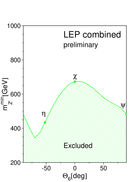
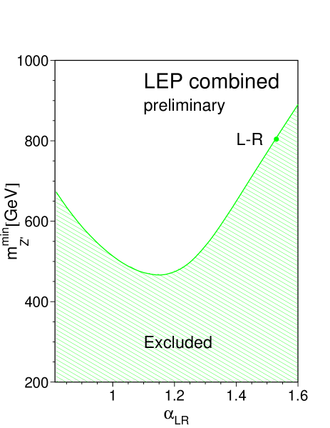
Figure 8.10: The 95% confidence level limits on $\mathrm{M}_{\mathrm{Z}^{{}^{\prime}}}$ as a function of the model parameter $\theta_{6}$ for E₆ models and $\alpha_{\mathrm{LR}}$ for left-right models. The Z-$\mathrm{Z^{\prime}}$ mixing is fixed, $\mbox{$\Theta_{\mathrm{Z}\mathrm{Z}^{{}^{\prime}}}$}=0$.

Z′ model	$\chi$	$\psi$	$\eta$	L-R	SSM
M${}_{Z^{\prime}}^{limit}$ (GeV/c2)	673	481	434	804	1787

Table 8.15: The 95% confidence level lower limits on the $\mathrm{Z^{\prime}}$ mass for $\chi,\leavevmode\nobreak\ \psi,\leavevmode\nobreak\ \eta$, L-R and SSM models.

8.5.3 Leptoquarks and R-parity violating squarks

Leptoquarks (LQ) would mediate quark-lepton transitions. Following the notations in Reference [94, 95], scalar leptoquarks, $S_{I}$, and vector leptoquarks,$V_{I}$ are indicated based on spin and isospin $I$. Leptoquarks with the same Isospin but with different hypercharges are distinguished by an additional tilde. See Reference 95 for further details. They carry fermion numbers, $F=L+3B$. It is assumed that leptoquark couplings to quark-lepton pairs preserve baryon- and lepton-number. The couplings $g_{L},\leavevmode\nobreak\ g_{R}$, are labelled according to the chirality of the lepton.

$\mathrm{\tilde{S}_{1/2}(L)}$ and $\mathrm{S_{0}(L})$ leptoquarks are equivalent to up-type anti-squarks and down-type squarks, respectively. Limits in terms of the leptoquark coupling are then exactly equivalent to limits on $\mathrm{\lambda}_{1jk}$ in the Lagrangian ${\mathrm{\lambda}_{1jk}L_{1}Q_{j}\bar{D}_{k}}$.

At LEP, the exchange of a leptoquark can modify the hadronic cross-sections and asymmetries, as described at the Born level by the equations given in Reference 95. Using the LEP combined measurements of hadronic cross-sections, and the measurements of heavy quark production, $R_{\mathrm{b}}$, $R_{\mathrm{c}}$, $A_{\mathrm{FB}}^{\mathrm{b\overline{b}}}$ and $A_{\mathrm{FB}}^{\mathrm{c\overline{c}}}$, upper limits can be set on the leptoquark’s coupling $g$ as a function of its mass $M_{\mathrm{L}Q}$ for leptoquarks coupling electrons to first, second and third generation quarks. For convenience, one type of leptoquark is assumed to be much lighter than the others. Furthermore, experimental constraints on the product $g_{L}g_{R}$ allow the study leptoquarks assuming either only $g_{L}\neq 0$ or $g_{R}\neq 0$. Limits are then denoted by either (L) for leptoquarks coupling to left handed leptons or (R) for leptoquarks coupling to right handed leptons.

In the processes $\mathrm{e}^{+}\mathrm{e}^{-}\rightarrow\mathrm{u\overline{u}}$ and $\mathrm{e}^{+}\mathrm{e}^{-}\rightarrow\mathrm{d\overline{d}}$ first generation leptoquarks could be exchanged in $u$- or $t$-channel (F=2 or F=0) which would lead to a change of the hadronic cross-section. In the processes $\mathrm{e}^{+}\mathrm{e}^{-}\rightarrow\mathrm{c\overline{c}}$ and $\mathrm{e}^{+}\mathrm{e}^{-}\rightarrow\mathrm{b\overline{b}}$ the exchange of leptoquarks with cross-generational couplings can alter the $\mathrm{q\overline{q}}$ angular distribution, especially at low polar angle. The reported measurements on heavy quark production have been extrapolated to $4\pi$ acceptance, using SM predictions, from the measurements performed in restricted angular ranges, corresponding to the acceptance of the vertex-detector in each experiment. Therefore, when fitting limits on leptoquarks’ coupling to the 2nd or 3rd generation of quarks, the LEP combined results for b and c sector are extrapolated back to an angular range of $\left|\cos\theta\right|<0.85$ using ZFITTER predictions.

The following measurements are used to constrain different types of leptoquarks

• For leptoquarks coupling electrons to 1^st generation quarks, all LEP combined hadronic cross-sections at centre-of-mass energies from 130 GeV to 207 GeV are used

• For leptoquarks coupling electrons to 2^nd generation quarks, $\sigma_{\mathrm{c\overline{c}}}$ is calculated from $R_{\mathrm{c}}$ and the hadronic cross-section at the energy points where $R_{\mathrm{c}}$ is measured. The measurements of $\sigma_{\mathrm{c\overline{c}}}$ and $A_{\mathrm{FB}}^{\mathrm{c\overline{c}}}$ are then extrapolated back to $\left|\cos\theta\right|<0.85$. Since measurements in the c-sector are scarce and originate from, at most, 2 experiments, hadronic cross-sections, extrapolated down to $\left|\cos\theta\right|<0.85$ are also used in the fit, with an average $10\%$ correlated errors.

• For leptoquarks coupling electrons to 3^rd generation quarks, only ${\mathrm{\sigma}_{b\bar{b}}}$ and $A_{\mathrm{FB}}^{\mathrm{b\overline{b}}}$, extrapolated back to a $\left|\cos\theta\right|<0.85$ are used.

The 95$\%$ confidence level lower limits on masses $M_{\mathrm{L}Q}$ are derived assuming a coupling of electromagnetic strength, $g=\sqrt{4\pi\alpha_{em}}$, where $\alpha_{em}$ is the fine structure constant. The results are summarised in Table 8.16. These results complement the leptoquark searches at HERA [96, 97] and the Tevatron [98]. Figures 8.11 and 8.12 give the 95% confidence level limits on the coupling as a function of the leptoquark mass for leptoquarks coupling electrons to the second and third generations of quarks.

Limit on scalar LQ mass (GeV/$c^{2}$)
	$\mathrm{S_{0}(L})$	$\mathrm{S_{0}(R)}$	$\mathrm{\tilde{S}_{0}(R)}$	$\mathrm{S_{\mbox{\tiny$\frac{1}{2}$}}(L})$	$\mathrm{S_{\mbox{\tiny$\frac{1}{2}$}}(R)}$	$\mathrm{\tilde{S}_{\mbox{\tiny$\frac{1}{2}$}}(L)}$	$\mathrm{S_{1}(L})$
$LQ_{1st}$	655	520	202	178	232	-	361
$LQ_{2nd}$	539	430	285	269	309	-	478
$LQ_{3rd}$	NA	NA	465	NA	389	107	1050
Limit on vector LQ mass (GeV/$c^{2}$)
	$\mathrm{V_{0}(L)}$	$\mathrm{V_{0}(R)}$	$\mathrm{\tilde{V}_{0}(R)}$	$\mathrm{V_{\mbox{\tiny$\frac{1}{2}$}}(L)}$	$\mathrm{V_{\mbox{\tiny$\frac{1}{2}$}}(R)}$	$\mathrm{\tilde{V}_{\mbox{\tiny$\frac{1}{2}$}}(L)}$	$\mathrm{V_{1}(L)}$
$LQ_{1st}$	917	165	489	303	227	176	659
$LQ_{2nd}$	692	183	630	357	256	187	873
$LQ_{3rd}$	829	170	NA	451	183	NA	829

Table 8.16: $95\%$ confidence level lower limits on the LQ mass for leptoquarks coupling between electrons and the first, second and third generation of quarks. A dash indicates that no limit can be set and N.A denotes leptoquarks coupling only to top quarks and hence not visible at LEP.

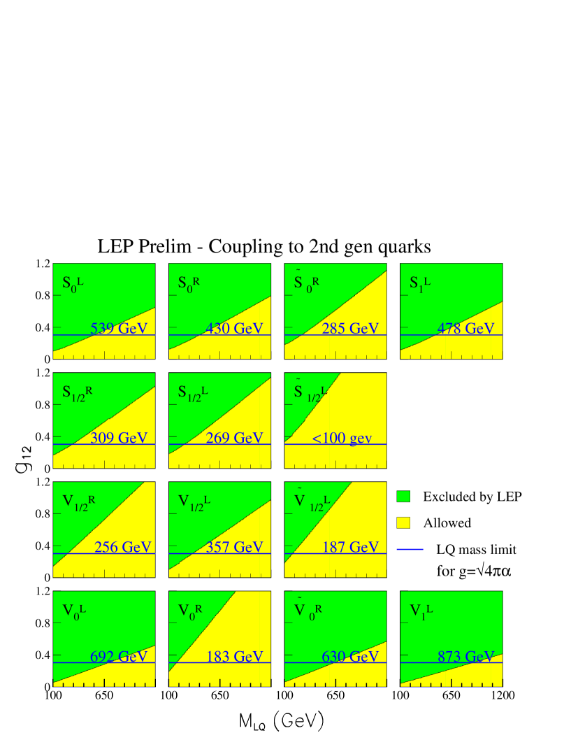
Figure 8.11: 95% confidence level limit on the coupling of leptoquarks to 2nd generation of quarks.

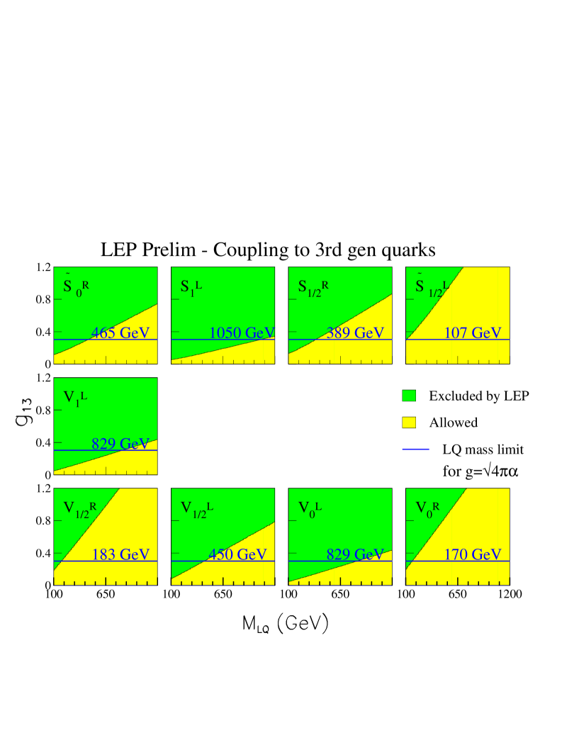
Figure 8.12: 95% confidence level limit on the coupling of leptoquarks to 3rd generation of quarks.

8.5.4 Low Scale Gravity in Large Extra Dimensions

The averaged differential cross-sections for $\mathrm{e}^{+}\mathrm{e}^{-}\rightarrow\mathrm{e}^{+}\mathrm{e}^{-}$ are used to search for the effects of graviton exchange in large extra dimensions.

A new approach to the solution of the hierarchy problem has been proposed in [99, 100, 101], which brings close the electroweak scale $\rm m_{EW}\sim 1\;TeV$ and the Planck scale $\rm M_{Pl}=\frac{1}{\sqrt{G_{N}}}\sim 10^{15}\;TeV$. In this framework the effective 4 dimensional $\rm M_{Pl}$ is connected to a new $\rm M_{Pl(4+n)}$ scale in a (4+n) dimensional theory:

$$\mathrm{M_{Pl}^{2}\sim M_{Pl(4+n)}^{2+n}R^{n}},$$ (8.4)

where there are n extra compact spatial dimensions of radius $\rm\sim R$.

In the production of fermion- or boson-pairs in $\mathrm{e}^{+}\mathrm{e}^{-}$ collisions this class of models can be manifested through virtual effects due to the exchange of gravitons (Kaluza-Klein excitations). As discussed in [102, 103, 104, 105, 106], the exchange of spin-2 gravitons modifies in a unique way the differential cross-sections for fermion pairs, providing clear signatures. These models introduce an effective scale (ultraviolet cut-off). Adopting the notation from [102] the gravitational mass scale is called $\mathrm{M_{H}}$. The cut-off scale is supposed to be of the order of the fundamental gravity scale in 4+n dimensions.

The parameter $\varepsilon_{H}$ is defined as

$$\varepsilon_{H}=\frac{\lambda}{\mathrm{M_{H}^{4}}},$$ (8.5)

where the coefficient $\rm\lambda$ is of $\rm\mathcal{O}(1)$ and can not be calculated explicitly without knowledge of the full quantum gravity theory. In the following analysis we will assume that $\rm\lambda=\pm 1$ in order to study both the cases of positive and negative interference. To compute the deviations from the Standard Model due to virtual graviton exchange the calculations [104, 103] were used.

Theoretical uncertainties on the Standard Model predictions are taken from [79]. The full correlation matrix of the differential cross-sections, obtained in our averaging procedure, is used in the fits. This is an improvement compared to previous combined analyses of published or preliminary LEP data on Bhabha scattering, performed before this detailed information was available (see e.g. [107, 108, 109]).

The extracted value of $\varepsilon_{H}$ is compatible with the Standard Model expectation $\varepsilon_{H}=0$. The errors on $\varepsilon_{H}$ are $\sim 1.5$ smaller than those obtained from a single LEP experiment with the same data set. The fitted value of $\varepsilon_{H}$ is converted into $95\%$ confidence level lower limits on $\mathrm{M_{H}}$ by integrating the likelihood function over the physically allowed values, $\varepsilon_{H}\geq 0$ for $\lambda=+1$ and $\varepsilon_{H}\leq 0$ for $\lambda=-1$ giving:

$$\mathrm{M_{H}} > 1.20\leavevmode\nobreak\ {\mathrm{Te\kern-1.00006ptV}}\qquad\mathrm{for}\leavevmode\nobreak\ \lambda=+1\,,$$ (8.6)

$$\mathrm{M_{H}} > 1.09\leavevmode\nobreak\ {\mathrm{Te\kern-1.00006ptV}}\qquad\mathrm{for}\leavevmode\nobreak\ \lambda=-1\,.$$ (8.7)

An example of our analysis for the highest energy point is shown in Figure 8.13.

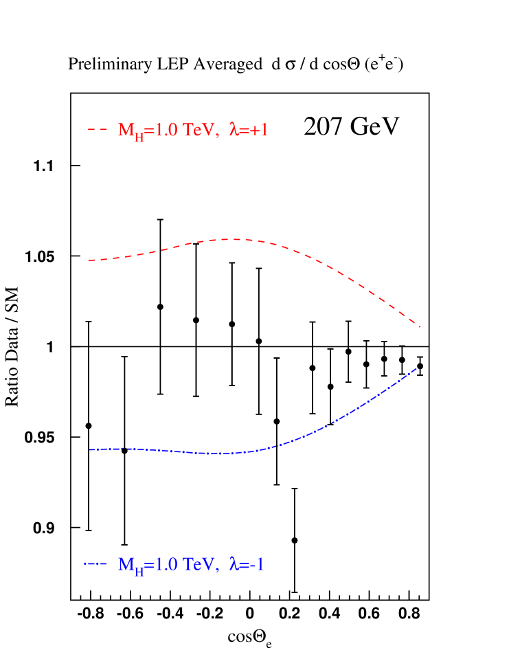
Figure 8.13: Ratio of the LEP averaged differential cross-section for $\mathrm{e}^{+}\mathrm{e}^{-}\rightarrow\mathrm{e}^{+}\mathrm{e}^{-}$ at energy of 207 ${\mathrm{Ge\kern-1.00006ptV}}$ compared to the SM prediction. The effects expected from virtual graviton exchange are also shown.

The interference of virtual graviton exchange amplitudes with both t-channel and s-channel Bhabha scattering amplitudes makes this the most sensitive search channel at LEP. The results obtained here would not be strictly valid if the luminosity measurements of the LEP experiments, based on the very same process, are also significantly affected by graviton exchange. As shown in [107], the effect on the cross-section in the luminosity angular range is so small that it can safely be neglected in this analysis.

8.6 Summary

A preliminary combination of the LEP-II $\mathrm{e}^{+}\mathrm{e}^{-}\rightarrow\mathrm{f\overline{f}}$ cross-sections (for hadron, muon and tau-lepton final states) and forward-backward asymmetries (for muon and tau final states) from LEP running at energies from 130 ${\mathrm{Ge\kern-1.00006ptV}}$ to 207 ${\mathrm{Ge\kern-1.00006ptV}}$ has been made. The results from the four LEP experiments are in good agreement with each other. The averages for all energies are shown given in Table 8.2. Overall the data agree with the Standard Model predictions of ZFITTER, although the combined hadronic cross-sections are on average $1.7$ standard deviations above the predictions. Further information is available at [77].

Preliminary differential cross-sections, $\frac{{\mathrm{d}}\sigma}{{\mathrm{d}}\cos\theta}$, for $\mathrm{e}^{+}\mathrm{e}^{-}\rightarrow\mathrm{e}^{+}\mathrm{e}^{-}$, $\mathrm{e}^{+}\mathrm{e}^{-}\rightarrow\mu^{+}\mu^{-}$ and $\mathrm{e}^{+}\mathrm{e}^{-}\rightarrow\tau^{+}\tau^{-}$ were combined. Results are shown in Figures 8.4, 8.5 and 8.6.

A preliminary average of results on heavy flavour production at LEP-II has also been made for measurements of $R_{\mathrm{b}}$, $R_{\mathrm{c}}$, $A_{\mathrm{FB}}^{\mathrm{b\overline{b}}}$ and $A_{\mathrm{FB}}^{\mathrm{c\overline{c}}}$, using results from LEP centre-of-mass energies from 130 to 207 ${\mathrm{Ge\kern-1.00006ptV}}$. Results are given in Tables 8.9 and 8.10 and shown graphically in Figures 8.7 and 8.8. The results are in good agreement with the predictions of the SM.

The preliminary averaged cross-section and forward-backward asymmetry results together with the combined results on heavy flavour production have been interpreted in a variety of models. Limits on the scale of contact interactions between leptons and quarks and in $\mathrm{e}^{+}\mathrm{e}^{-}\rightarrow\mathrm{e}^{+}\mathrm{e}^{-}$ and also between electrons and specifically $\mathrm{b\overline{b}}$ and $\mathrm{c\overline{c}}$ final states have been determined. A full set of limits are given in Tables 8.13 and 8.14. The LEP-II averaged cross-sections have been used to obtain lower limits on the mass of a possible $\mathrm{Z^{\prime}}$ boson in different models. Limits range from $340$ to $1787$ ${\mathrm{Ge\kern-1.00006ptV}}/c^{2}$ depending on the model. Limits on the masses of leptoquarks have been derived from the hadronic cross-sections. The limits range from $101$ to $1036$ ${\mathrm{Ge\kern-1.00006ptV}}/c^{2}$ depending on the type of leptoquark. Limits on the scale of gravity in models with large extra dimensions have been obtained from combined differential cross-sections for $\mathrm{e}^{+}\mathrm{e}^{-}\rightarrow\mathrm{e}^{+}\mathrm{e}^{-}$; for positive interference between the new physics and the Standard model the limit is $1.20$ TeV and for negative interference $1.09$ TeV.

Chapter 9 Investigation of the Photon/Z-Boson Interference

Updates with respect to summer 2003:
Unchanged w.r.t. summer 2002: Results are preliminary.

9.1 Introduction

The S-Matrix ansatz provides a coherent way of describing LEP measurements of the cross-section and forward-backward asymmetries in $s$-channel $\mathrm{e}^{+}\mathrm{e}^{-}\rightarrow\mathrm{f\overline{f}}$ processes at centre-of-mass energies around the $\mathrm{Z}$ resonance, from the LEP-I program, and the measurements at centre-of-mass energies from 130 – 207 GeV from the LEP-II program.

Compared with the standard 5 and 9 parameter descriptions of the measurements at the $\mathrm{Z}$ [110], the S-Matrix formalism includes an extra 3 parameters (assuming lepton universality) or 7 parameters (without lepton universality) which explicitly determine the contributions to the cross-sections and forward-backward asymmetries of the interference between the exchange of a $\mathrm{Z}$ and a photon. The LEP-I data alone cannot tightly constrain these interference terms, in particular the interference term for hadronic cross-sections, since their contributions are small around the $\mathrm{Z}$ resonance and change sign at the pole. Due to strong correlations between the size of the hadronic interference term and the mass of the $\mathrm{Z}$, this leads to a larger error on the fitted mass of the $\mathrm{Z}$ compared to the standard 5 and 9 parameter fits, where the hadronic interference term is fixed to the value predicted in the Standard Model. Including the LEP-II data leads to a significant improvement in the constraints on the interference terms and a corresponding reduction in the uncertainty on the mass of the $\mathrm{Z}$. This results in a measurement of $m_{\mathrm{Z}}$ which is almost as sensitive as the standard results, but without constraining the interference to the Standard Model prediction.

This chapter describes the first, preliminary, combination of data from the full data sets of the 4 LEP experiments, to obtain a LEP combined results on the parameters of the S-Matrix ansatz. These results update those of a previous combination [111] which was based on preliminary LEP-I data and only partial statistics from the full LEP-II data set.

Different strategies are used to combined the LEP-I and LEP-II data. For LEP-I data, an average of the individual experiment’s results on the S-Matrix parameters is made. This approach is rather similar to the method used to combine the results of the 5 and 9 parameter fits. To include LEP-II data, a fit is made to LEP combined measurements of cross-sections and asymmetries above the $\mathrm{Z}$, taking into account the results of the LEP-I combination of S-Matrix parameters.

In Section 9.2 the parameters of the S-Matrix ansatz are explained. In Sections 9.3.1 and 9.3.2 the average of the LEP-I data and the inclusion of the LEP-II data are described. The results are discussed in Section 9.3.3 and conclusions are drawn in Section 9.4.

9.2 The S-Matrix Ansatz

The S-matrix ansatz [112] is a rigorous approach to describe the cross-sections and forward-backward asymmetries in the $s$-channel $\mathrm{e}^{+}\mathrm{e}^{-}$ annihilations under the assumption that the processes can be parameterised as the exchange of a massless and a massive vector boson, in which the couplings of the bosons including their interference are treated as free parameters.

In this model, the cross-sections can be parametrised as follows:

$$\sigma^{0}_{tot,f}(s)=\frac{4}{3}\pi\alpha^{2}\left[\frac{{g}_{\mathrm{f}}^{tot}}{s}+\frac{{j}_{\mathrm{f}}^{tot}(s-\overline{m}_{\mathrm{Z}}^{2})+{r}_{\mathrm{f}}^{tot}\,s}{(s-\overline{m}_{\mathrm{Z}}^{2})^{2}+\overline{m}_{\mathrm{Z}}^{2}\overline{\Gamma}_{\mathrm{Z}}^{2}}\right]\,\,\,\mathrm{with}\,\,\mathrm{f=had,e,\mu,\tau}\,,$$ (9.1)

while the forward-backward asymmetries are given by:

$$A^{0}_{\mathrm{fb,f}}(s)=\pi\alpha^{2}\left[\frac{{g}_{\mathrm{f}}^{fb}}{s}+\frac{{j}_{\mathrm{f}}^{fb}(s-\overline{m}_{\mathrm{Z}}^{2})+{r}_{\mathrm{f}}^{fb}\,s}{(s-\overline{m}_{\mathrm{Z}}^{2})^{2}+\overline{m}_{\mathrm{Z}}^{2}\overline{\Gamma}_{\mathrm{Z}}^{2}}\right]/{\sigma^{0}_{\mathrm{tot,f}}(s)}\,,$$ (9.2)

where $\sqrt{s}$ is the centre-of-mass energy. The parameters ${r}_{\mathrm{f}}$ and ${j}_{\mathrm{f}}$ scale the $\mathrm{Z}$ exchange and the $\mathrm{Z}-\gamma$ interference contributions to the total cross-section and forward-backward asymmetries. The contribution ${g}_{\mathrm{f}}$ of the pure $\gamma$ exchange was fixed to the value predicted by QED in all fits. Neither the hadronic charge asymmetry, nor the flavour tagged quark forward-backward asymmetries are considered here, which leaves 16 free parameters to described the LEP data: 14 ${r}_{\mathrm{f}}$ and ${j}_{\mathrm{f}}$ parameters and the mass and width of the massive $\mathrm{Z}$ resonance. Applying the constraint of lepton universality reduces this to 8 parameters.

In the Standard Model the $\mathrm{Z}$ exchange term, the $\mathrm{Z}-\gamma$ interference term and the photon exchange term are given in terms of the fermion charges and their effective vector and axial couplings to the $\mathrm{Z}$ by:

$$\begin{array}[]{l@{}l@{}l@{}l}\displaystyle r^{\mathrm{tot}}_{\mathrm{f}}&=&\kappa^{2}\left[g_{\mathrm{Ae}}^{2}+g_{\mathrm{Ve}}^{2}\rule{0.0pt}{11.38109pt}\right]\left[g_{\mathrm{Af}}^{2}+g_{\mathrm{Vf}}^{2}\right]-2\kappa\,g_{\mathrm{Ve}}\,g_{\mathrm{Vf}}C_{Im}\\[14.22636pt] j\mathrm{{}^{tot}_{f}}&=&2\kappa\,g_{\mathrm{Ve}}\,g_{\mathrm{Vf}}\left(C_{Re}+C_{Im}\right)\\[14.22636pt] g\mathrm{{}^{tot}_{f}}&=&Q^{2}_{\mathrm{e}}Q^{2}_{\mathrm{f}}\left|F_{A}(m_{\mathrm{Z}})\right|^{2}\\[14.22636pt] r\mathrm{{}^{fb}_{f}}&=&4\kappa^{2}g_{\mathrm{Ae}}\,g_{\mathrm{Ve}}\,g_{\mathrm{Af}}\,g_{\mathrm{Vf}}-2\kappa\,g_{\mathrm{Ae}}\,g_{\mathrm{Af}}C_{Im}\\[14.22636pt] j\mathrm{{}^{fb}_{f}}&=&2\kappa\,g_{\mathrm{Ae}}\,g_{\mathrm{Af}}\left(C_{Re}+C_{Im}\right)\\[14.22636pt] g\mathrm{{}^{fb}_{f}}&=&0\,,\end{array}$$ (9.3)

with the following definitions:

$$\begin{array}[]{l}\displaystyle\kappa=\frac{\displaystyle G_{F}m_{\mathrm{Z}}^{2}}{\displaystyle 2\sqrt{2\,}\pi\alpha}\approx 1.50\\[14.22636pt] C_{Im}=\frac{\displaystyle\Gamma_{\mathrm{Z}}}{\displaystyle m_{\mathrm{Z}}}\left.Q_{\mathrm{e}}Q_{\mathrm{f}}\right.\mathrm{Im}\left\{F_{A}(m_{\mathrm{Z}})\right\}\\[14.22636pt] C_{Re}=\left.Q_{\mathrm{e}}Q_{\mathrm{f}}\right.\mathrm{Re}\left\{F_{A}(m_{\mathrm{Z}})\right\}\\[14.22636pt] F_{A}(m_{\mathrm{Z}})=\frac{\displaystyle\alpha(m_{\mathrm{Z}})}{\displaystyle\alpha}\,,\end{array}$$ (9.4)

where $\alpha(m_{\mathrm{Z}})$ is the complex fine-structure constant, and $\alpha\equiv\alpha(0)$. The photonic virtual and bremsstrahlung corrections are included through the convolution of Equations 9.1 and 9.2 with radiator functions as in the 5 and 9 parameter fits. The expressions of the S-Matrix parameters in terms of the effective vector and axial-vector couplings given above neglect the imaginary parts of the effective couplings.

The usual definitions of the mass $m_{\mathrm{Z}}$ and width $\Gamma_{\mathrm{Z}}$ of a Breit-Wigner resonance are used, the width being $s$-dependent, such that:

$$\begin{array}[]{lllll@{}c@{}r}m_{\mathrm{Z}}&\equiv&\overline{m}_{\mathrm{Z}}\sqrt{1+\overline{\Gamma}_{\mathrm{Z}}^{2}/\overline{m}_{\mathrm{Z}}^{2}}&\approx&\overline{m}_{\mathrm{Z}}&+&34.20\leavevmode\nobreak\ {\mathrm{Me\kern-1.00006ptV}}/c^{2}\phantom{\,,}\\[8.53581pt] \Gamma_{\mathrm{Z}}&\equiv&\overline{\Gamma}_{\mathrm{Z}}\sqrt{1+\overline{\Gamma}_{\mathrm{Z}}^{2}/\overline{m}_{\mathrm{Z}}^{2}}&\approx&\overline{\Gamma}_{\mathrm{Z}}&+&0.94\leavevmode\nobreak\ {\mathrm{Me\kern-1.00006ptV}}\,.\phantom{/c^{2}}\end{array}$$ (9.5)

In the following fits, the predictions from the S-Matrix ansatz and the QED convolution for cross-sections and asymmetries are made using SMATASY [116], which in turn uses ZFITTER [117] to calculate the QED convolution of the electroweak kernel. In case of the $\mathrm{e}^{+}\mathrm{e}^{-}$ final state, $t$-channel and $s/t$ interference contributions are added to the $s$-channel ansatz.

9.3 LEP combination

In the following sections the combinations of the results from the individual LEP experiments are described: firstly the LEP-I combination, then the combination of both LEP-I and LEP-II data. The results from these combinations are compared in Section 9.3.3. Although all 16 parameters are averaged during the combination, only results for the parameters $m_{\mathrm{Z}}$ and $j\mathrm{{}^{tot}_{had}}$ are reported here. Systematic studies specific to the other parameters are ongoing.

9.3.1 LEP-I combination

Individual LEP experiments have their own determinations of the 16 S-Matrix parameters [118, 119, 120, 121] from LEP-I data alone, using the full LEP-I data sets.

These results are averaged using a multi-parameter BLUE technique based on an extension of Reference 81. Sources of systematic uncertainty correlated between the experiments have been investigated, using techniques described in [110] and are accounted for in the averaging procedure and benefiting from the experience gained in those combinations.

The parameters $m_{\mathrm{Z}}$ and $j\mathrm{{}^{tot}_{had}}$ are the most sensitive of all 16 S-matrix parameters to the inclusion of the LEP-II data, and are also the most interesting ones in the context of the 5 and 9 parameter fits. For these parameters the most significant source of systematic error which is correlated between experiments comes from the uncertainty on the $\mathrm{e}^{+}\mathrm{e}^{-}$ collision energy as determined by models of the LEP RF system and calibrations using the resonant depolarisation technique. These errors amount to $\pm 3$ MeV on $m_{\mathrm{Z}}$ and $\pm 0.16$ on $j\mathrm{{}^{tot}_{had}}$ with a correlation coefficient of $-0.86$. The LEP averaged values of $m_{\mathrm{Z}}$ and $j\mathrm{{}^{tot}_{had}}$ are given in Table 9.1, together with their correlation coefficient. The $\chi^{2}/$D.O.F. for the average of all 16 parameters is 62.0/48, corresponding to a probability of $8\%$, which is acceptable.

	$m_{\mathrm{Z}}$ [GeV]		$j\mathrm{{}^{tot}_{had}}$		correlation
LEP-I only	91.1925$\pm$	0.0059	-0.084$\pm$	0.324	-0.935
LEP-I & LEP-II	91.1869$\pm$	0.0023	0.277$\pm$	0.065	-0.461

Table 9.1: Averaged LEP-I and LEP-II S-Matrix results for $m_{\mathrm{Z}}$ and $j\mathrm{{}^{tot}_{had}}$.

9.3.2 LEP-I and LEP-II combination

Some experiments have determined S-Matrix parameters using their LEP-I and LEP-II measured cross-sections and forward-backward asymmetries [118, 119, 122, 123]. To do a full LEP combination would require each experiment to provide S-Matrix results and would require an analysis of the correlated systematic errors on each measured parameter.

However, preliminary combinations of the measurements of forward-backward asymmetries and cross-sections from all 4 LEP experiments, for the full LEP-II period, have already been made [117] and correlations between these measurements have been estimated. The combination procedure averages measurements of cross-sections and asymmetry for those events with reduced centre-of-mass energies, $\sqrt{s^{\prime}}$, close to the actual centre-of-mass energy of the $\mathrm{e}^{+}\mathrm{e}^{-}$ beams, $\sqrt{s}$, removing those events which are less sensitive to the $\mathrm{Z}-\gamma$ interference where, predominantly, initial state radiation reduces the centre-of-mass energy to close to the mass of the $\mathrm{Z}$. The only significant correlations are those between hadronic cross-section measurements at different energies, which are around 20–40%, depending on energies.

The predictions from SMATASY are fitted to the combined LEP-II cross-section and forward-backward asymmetry measurements [117]. The signal definition 1 of Reference 117 is used for the data and for the predictions of SMATASY. Theoretical uncertainties on the S-Matrix predictions for the LEP-II results and on the corrections of the LEP II data to the common signal defintion are taken to be the same as for the Standard Model predictions of ZFITTER [117] which are dominated by uncertainties in the QED convolution. These amount to a relative uncertainty of $0.26\%$ on the hadronic cross-sections, fully correlated between all LEP-II energies.

The fit also uses as inputs the averaged LEP-I S-Matrix parameters and covariance matrix. These inputs effectively constrain those parameters, such as $m_{\mathrm{Z}}$, which are not accurately determined by LEP-II data. There are no significant correlations between the LEP-I and LEP-II inputs.

The LEP averaged values of $m_{\mathrm{Z}}$ and $j\mathrm{{}^{tot}_{had}}$ for both LEP-I and LEP-II data are given in Table 9.1, together with their correlation coefficient. The $\chi^{2}/$D.O.F. for the average of all 16 parameters is 64.4/60, corresponding to a probability of $33\%$, which is good.

9.3.3 Discussion

In the LEP-I combination the measured values of the Z boson mass $m_{\mathrm{Z}}=91.1925\pm 0.0059$ GeV agrees well with the results of the standard 9 parameter fit ($91.1876\pm 0.0021$ GeV) albeit with a significantly larger error, resulting from the correlation with the large uncertainty on $j\mathrm{{}^{tot}_{had}}$ which is then the dominant source of uncertainty on $m_{\mathrm{Z}}$ in the S-Matrix fits. The measured value of $j\mathrm{{}^{tot}_{had}}=-0.084\pm 0.324$ , also agrees with the prediction of the Standard Model ($0.2201^{+0.0032}_{-0.0137}$).

Including the LEP-II data brings a significant improvement in the uncertainty on the size of the interference between $\mathrm{Z}$ and photon exchange compared to LEP-I data alone. The measured value $j\mathrm{{}^{tot}_{had}}=0.277\pm 0.065$, agrees well with the values predicted from the Standard Model. Correspondingly, the uncertainty on the the mass of the $\mathrm{Z}$ in this ansatz, $2.3$ MeV, is close to the precision obtained from LEP-I data alone using the standard 9 parameter fit, $2.1$ MeV. The slightly larger error is due to the uncertainty on $j\mathrm{{}^{tot}_{had}}$ which amounts to 0.9 MeV. The measured value, $m_{\mathrm{Z}}=91.1869\pm 0.0023$ GeV, agrees with that obtained from the standard 9 parameter fits. The results are summarised in Figure 9.1.

The good agreement found between the values of $m_{\mathrm{Z}}$ and $j\mathrm{{}^{tot}_{had}}$ and their expectations provide a validation of the approach taken in the standard 5 and 9 parameter fits, in which the size of the interference between $\mathrm{Z}$ boson and photon exchange in the hadronic cross-sections was fixed to the Standard Model expectation.

The precision on $j\mathrm{{}^{tot}_{had}}$ is slightly better than that obtained by the VENUS collaboration [124] of $\pm 0.08$, which was obtained using preliminary results from LEP-I and their own measurements of the hadronic cross-section below the $\mathrm{Z}$ resonance. The measurement of the hadronic cross-sections from VENUS [124] and TOPAZ [125] could be included in the future to give a further reduction in the uncertainty on $j\mathrm{{}^{tot}_{had}}$.

Work is in progress to understand those sources of systematic error, correlated between experiments, which are significant for the remaining S-Matrix parameter that have not been presented here. In particular, for $j\mathrm{{}^{tot}_{e}}$ and $j\mathrm{{}^{fb}_{e}}$, it is important to understand the errors resulting from $t$-channel contributions to the $\mathrm{e}^{+}\mathrm{e}^{-}\rightarrow\mathrm{e}^{+}\mathrm{e}^{-}$ process. These errors have only limited impact on the standard 5 and 9 parameter fits.

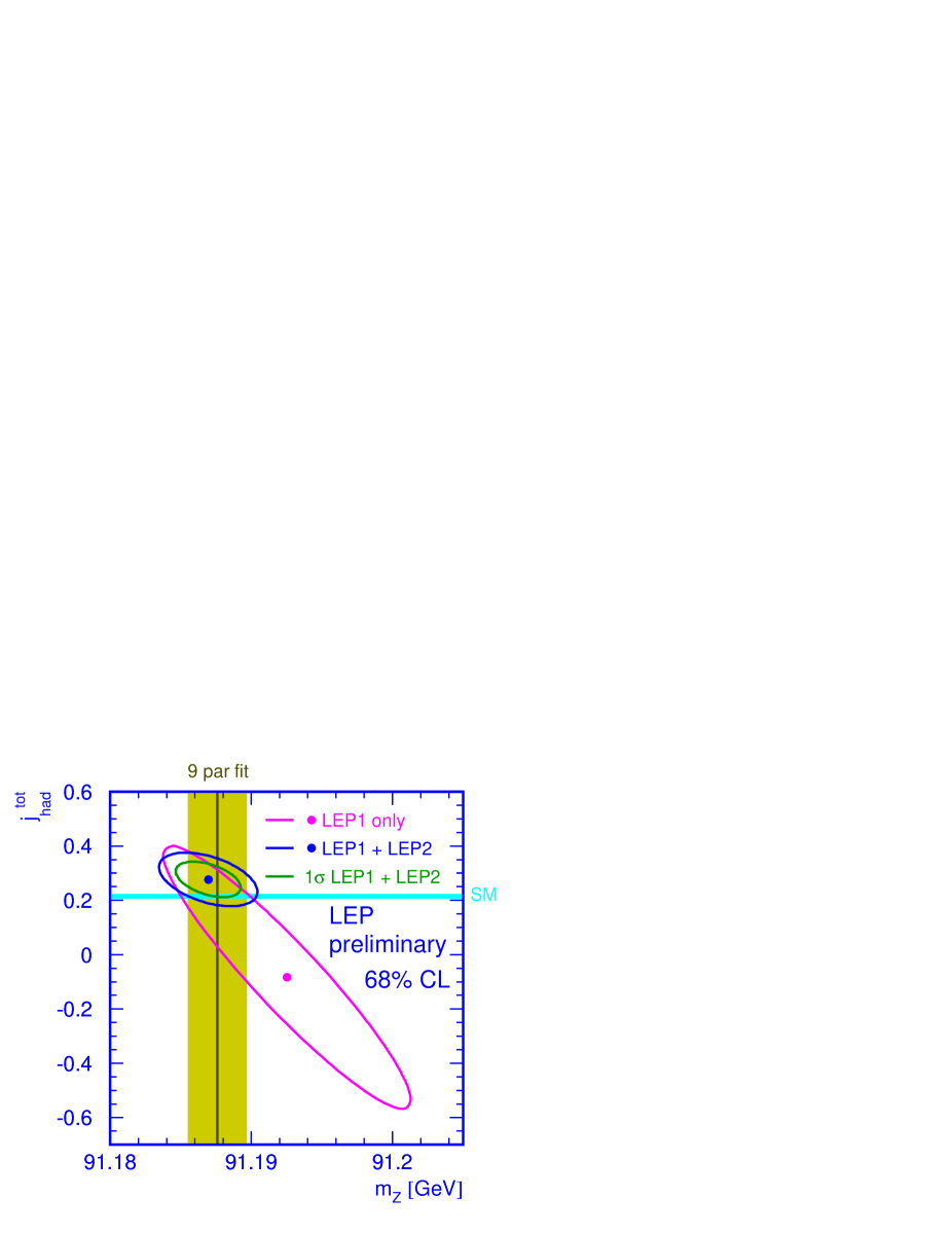
Figure 9.1: Error ellipses for $m_{\mathrm{Z}}$ and $j\mathrm{{}^{tot}_{had}}$ for LEP-I (at 39% and 68%) and the combination of LEP-I and LEP-II (at 68%).

9.4 Conclusion

Results for the S-Matrix parameter $m_{\mathrm{Z}}$ and $j\mathrm{{}^{tot}_{had}}$ have been presented for LEP-I data alone and for a fit using the full data sets for LEP-I and LEP-II from all 4 LEP experiments. Inclusion of LEP-II data brings a significant improvement in the determination of $j\mathrm{{}^{tot}_{had}}$, the fitted value $0.277\pm 0.065$, agrees well with the values predicted from the Standard Model. As a result in the improvement of the uncertainty in $j\mathrm{{}^{tot}_{had}}$, the uncertainty on the fitted value of $m_{\mathrm{Z}}$ approaches that of the standard 5 and 9 parameter fits and the measured value $m_{\mathrm{Z}}=91.1869\pm 0.0023$ GeV is compatible with that from the standard fits.

Chapter 10 W and Four-Fermion Production at LEP-II

Updates with respect to summer 2003:
The WW cross-section, ${\cal{R}}_{\mathrm{WW}}$ and the W branching ratios combinations are updated including the final ALEPH, DELPHI and L3 results. The determination of $|\mathrm{V}_{\mathrm{cs}}|$ is updated with new inputs from the PDG 2002 The ZZ cross-section and ${\cal{R}}_{\mathrm{ZZ}}$ combinations are updated accounting for the final DELPHI  L3 and OPAL results. The Zee cross-section and the corresponding ${\cal{R}}_{\mathrm{Zee}}$ combinations are updated with final ALEPH and L3 results. The single-W combination includes the final ALEPH and L3 results. All combinations are preliminary.

10.1 Introduction

This chapter summarises the present status of the combination of published and preliminary results of the four LEP experiments on four-fermion cross-sections for the Summer 2004 Conferences. If not stated otherwise, all presented results use the full LEP2 data sample at centre–of–mass energies up to 209 GeV, supersede the results presented at the Summer 2003 Conferences [126] and have to be considered as preliminary.

The centre–of–mass energies and the corresponding integrated luminosities are provided by the experiments and are the same used for previous conferences. The LEP energy value in each point (or group of points) is the luminosity-weighted average of those values.

Cross-section results from different experiments are combined by $\chi^{2}$ minimisation using the Best Linear Unbiased Estimate method described in Ref. [81], properly taking into account the correlations between the systematic uncertainties.

The detailed inputs from the experiments and the resulting LEP combined values, with the full breakdown of systematic errors is described in Appendix C. Experimental results are compared with recent theoretical predictions, many of which were developed in the framework of the LEP2 Monte Carlo workshop [127].

10.2 W-pair production cross-section

ALEPH, DELPHI and L3 have presented final results on the W-pair (CC03 [127]) production cross-section and W branching ratios for all LEP2 centre–of–mass energies [128, 129, 130, 131, 132]. OPAL has final results from 161 to 189 GeV [128, 129, 133] and preliminary measurements at $\sqrt{s}=192$–207 GeV [134].

With respect to the Summer 2003 Conferences, new final results from ALEPH and L3 are now included in the LEP averages. The same grouping of the systematic errors consolidated in previous combinations [126] was used.

The detailed inputs used for the combinations are given in Appendix C.

The measured statistical errors are used for the combination; after building the full 32$\times$32 covariance matrix for the measurements, the $\chi^{2}$ minimisation fit is performed by matrix algebra, as described in Ref. [135], and is cross-checked using Minuit [136].

The results from each experiment for the W-pair production cross-section are shown in Table 10.1, together with the LEP combination at each energy. All measurements assume Standard Model values for the W decay branching fractions. The results for centre–of–mass energies between 183 and 207 GeV, for which new LEP averages have been computed, supersede the ones presented in [126]. For completeness, the measurements at 161 and 172 GeV are also listed in the table.

$\sqrt{s}$	WW cross-section (pb)					$\chi^{2}/\textrm{d.o.f.}$
(GeV)	ALEPH	DELPHI	L3	OPAL	LEP
161.3	$\phantom{0}4.23\pm 0.75^{*}$	$\phantom{0}3.67^{\phantom{0}+\phantom{0}0.99\phantom{0}*}_{\phantom{0}-\phantom{0}0.87}$	$\phantom{0}2.89^{\phantom{0}+\phantom{0}0.82\phantom{0}*}_{\phantom{0}-\phantom{0}0.71}$	$\phantom{0}3.62^{\phantom{0}+\phantom{0}0.94\phantom{0}*}_{\phantom{0}-\phantom{0}0.84}$	$\phantom{0}3.69\pm 0.45\phantom{{}^{*}}^{*}$	$\left\}\hskip 5.69054pt\phantom{0}1.3\phantom{0}/\phantom{0}3\right.$
172.1	$11.7\phantom{0}\pm 1.3\phantom{0}^{*}$	$11.6\phantom{0}\pm 1.4\phantom{0}^{*}$	$12.3\phantom{0}\pm 1.4\phantom{0}^{*}$	$12.3\phantom{0}\pm 1.3\phantom{0}^{*}$	$12.0\phantom{0}\pm 0.7\phantom{0}\phantom{{}^{*}}^{*}$	$\left\}\hskip 5.69054pt\phantom{0}0.22/\phantom{0}3\right.$
182.7	$15.90\pm 0.63^{*}$	$16.07\pm 0.70^{*}$	$16.53\pm 0.72^{*}$	$15.43\pm 0.66^{*}$	$15.89\pm 0.35\phantom{{}^{*}}^{*}$	$\left\}\begin{array}[h]{rr}&\hbox{\multirowsetup 26.4/24}\\ &\\ &\\ &\\ &\\ &\\ &\\ &\\ \end{array}\right.$
188.6	$15.76\pm 0.36^{*}$	$16.09\pm 0.42^{*}$	$16.17\pm 0.41^{*}$	$16.30\pm 0.39^{*}$	$16.03\pm 0.21\phantom{{}^{*}}^{*}$
191.6	$17.10\pm 0.90\phantom{{}^{*}}^{*}$	$16.64\pm 1.00^{*}$	$16.11\pm 0.92\phantom{{}^{*}}^{*}$	$16.60\pm 0.99\phantom{{}^{*}}$	$16.56\pm 0.48\phantom{{}^{*}}$
195.5	$16.61\pm 0.54\phantom{{}^{*}}^{*}$	$17.04\pm 0.60^{*}$	$16.22\pm 0.57\phantom{{}^{*}}^{*}$	$18.59\pm 0.75\phantom{{}^{*}}$	$16.90\pm 0.31\phantom{{}^{*}}$
199.5	$16.90\pm 0.52\phantom{{}^{*}}^{*}$	$17.39\pm 0.57^{*}$	$16.49\pm 0.58\phantom{{}^{*}}^{*}$	$16.32\pm 0.67\phantom{{}^{*}}$	$16.75\pm 0.30\phantom{{}^{*}}$
201.6	$16.65\pm 0.71\phantom{{}^{*}}^{*}$	$17.37\pm 0.82^{*}$	$16.01\pm 0.84\phantom{{}^{*}}^{*}$	$18.48\pm 0.92\phantom{{}^{*}}$	$17.00\pm 0.41\phantom{{}^{*}}$
204.9	$16.79\pm 0.54\phantom{{}^{*}}^{*}$	$17.56\pm 0.59^{*}$	$17.00\pm 0.60\phantom{{}^{*}}^{*}$	$15.97\pm 0.64\phantom{{}^{*}}$	$16.78\pm 0.31\phantom{{}^{*}}$
206.6	$17.36\pm 0.43\phantom{{}^{*}}^{*}$	$16.35\pm 0.47^{*}$	$17.33\pm 0.47\phantom{{}^{*}}^{*}$	$17.77\pm 0.57\phantom{{}^{*}}$	$17.13\pm 0.25\phantom{{}^{*}}$

Table 10.1: W-pair production cross-section from the four LEP experiments and combined values at all recorded centre–of–mass energies. All results are preliminary, with the exception of those indicated by ^∗. The measurements between 183 and 207 GeV have been combined in one global fit, taking into account inter-experiment as well as inter-energy correlations of systematic errors. The results for the combined LEP W-pair production cross-section at 161 and 172 GeV are taken from [137, 138] respectively.

Figure 10.1 shows the combined LEP W-pair cross-section measured as a function of the centre–of–mass energy. The experimental points are compared with the theoretical calculations from YFSWW [139] and RACOONWW [140] between 155 and 215 GeV for $m_{\mathrm{W}}=80.35$ GeV. The two codes have been extensively compared and agree at a level better than 0.5% at the LEP2 energies [127]. The calculations above 170 GeV, based for the two programs on the so-called leading pole (LPA) or double pole approximations (DPA) [141], have theoretical uncertainties decreasing from 0.7% at 170 GeV to about 0.4% at centre–of–mass energies larger than 200 GeV, while in the threshold region, where the codes are run in Improved Born Approximation, a larger theoretical uncertainty of 2% is assigned [142]. This theoretical uncertainty is represented by the blue band in Figure 10.1. An error of 50 MeV on the W mass would translate into additional errors of 0.1% (3.0%) on the cross-section predictions at 200 GeV (161 GeV, respectively). All results, up to the highest centre–of–mass energies, are in agreement with the considered theoretical predictions.

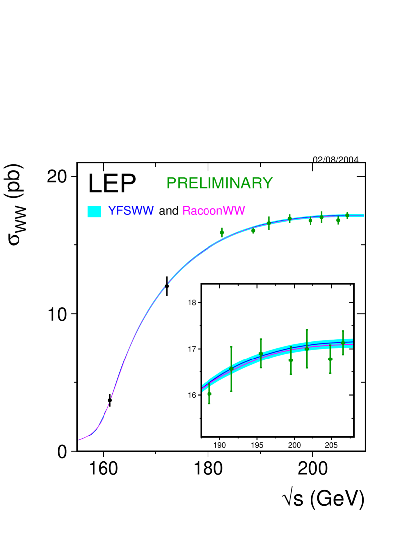
Figure 10.1: Measurements of the W-pair production cross-section, compared to the predictions of RACOONWW [140] and YFSWW [139]. The shaded area represents the uncertainty on the theoretical predictions, estimated in $\pm$2% for $\sqrt{s}\!<\!170$ GeV and ranging from 0.7 to 0.4% above 170 GeV.

The agreement between the measured W-pair cross-section, $\sigma_{\mathrm{WW}}^{\mathrm{meas}}$, and its expectation according to a given theoretical model, $\sigma_{\mathrm{WW}}^{\mathrm{theo}}$, can be expressed quantitatively in terms of their ratio

$${\cal{R}}_{\mathrm{WW}}=\frac{\sigma_{\mathrm{WW}}^{\mathrm{meas}}}{\sigma_{\mathrm{WW}}^{\mathrm{theo}}},$$ (10.1)

averaged over the measurements performed by the four experiments at different energies in the LEP2 region. The above procedure has been used to compare the measurements at the eight energies between 183 and 207 GeV to the predictions of GENTLE [143], KORALW [144], YFSWW [139] and RACOONWW [140]. The measurements at 161 and 172 GeV have not been used in the combination because they were performed using data samples of low statistics and because of the high sensitivity of the cross-section to the value of the W mass at these energies.

The combination of the ratio ${\cal{R}}_{\mathrm{WW}}$ is performed using as input from the four experiments the 32 cross-sections measured at each of the eight energies. These are then converted into 32 ratios by dividing them by the considered theoretical predictions, listed in Appendix C. The full 32$\times$32 covariance matrix for the ratios is built taking into account the same sources of systematic errors used for the combination of the W-pair cross-sections at these energies.

The small statistical errors on the theoretical predictions at the various energies, taken as fully correlated for the four experiments and uncorrelated between different energies, are also translated into errors on the individual measurements of ${\cal{R}}_{\mathrm{WW}}$. The theoretical errors on the predictions, due to the physical and technical precision of the generators used, are not propagated to the individual ratios but are used when comparing the combined values of ${\cal{R}}_{\mathrm{WW}}$ to unity. For each of the four models considered, two fits are performed: in the first, eight values of ${\cal{R}}_{\mathrm{WW}}$ at the different energies are extracted, averaged over the four experiments; in the second, only one value of ${\cal{R}}_{\mathrm{WW}}$ is determined, representing the global agreement of measured and predicted cross-sections over the whole energy range.

$\sqrt{s}$(GeV)	${\cal{R}}_{\mathrm{WW}}^{\footnotesize\mbox{YFSWW}}$	${\cal{R}}_{\mathrm{WW}}^{\footnotesize\mbox{RACOONWW}}$
182.7	$1.034\pm 0.023$	$1.034\pm 0.023$
188.6	$0.985\pm 0.013$	$0.986\pm 0.013$
191.6	$1.000\pm 0.029$	$1.003\pm 0.029$
195.5	$1.003\pm 0.019$	$1.006\pm 0.019$
199.5	$0.984\pm 0.018$	$0.986\pm 0.018$
201.6	$0.996\pm 0.024$	$0.998\pm 0.024$
204.9	$0.979\pm 0.018$	$0.982\pm 0.018$
206.6	$0.999\pm 0.015$	$1.003\pm 0.015$
$\chi^{2}$/d.o.f	26.4/24	26.4/24
Average	$0.993\pm 0.009$	$0.995\pm 0.009$
$\chi^{2}$/d.o.f	32.3/31	32.0/31

Table 10.2: Ratios of LEP combined W-pair cross-section measurements to the expectations according to YFSWW [139] and RACOONWW [140]. For each of the two models, two fits are performed, one to the LEP combined values of ${\cal{R}}_{\mathrm{WW}}$ at the eight energies between 183 and 207 GeV, and another to the LEP combined average of ${\cal{R}}_{\mathrm{WW}}$ over all energies. The results of the fits are given in the table together with the resulting $\chi^{2}$. Both fits take into account inter-experiment as well as inter-energy correlations of systematic errors.

      

Figure 10.2: Ratios of LEP combined W-pair cross-section measurements to the expectations according to YFSWW [139] and RACOONWW [140] The yellow bands represent constant relative errors of 0.5% on the two cross-section predictions.

The results of the two fits to ${\cal{R}}_{\mathrm{WW}}$ for YFSWW and RACOONWW are given in Table 10.2. As already qualitatively noted from Figure 10.1, the LEP measurements of the W-pair cross-section above threshold are in very good agreement to the predictions and can test the theory at the level of better than 1%. In contrast, the predictions from GENTLE and KORALW are about 3% too high with respect to the measurements; the equivalent values of ${\cal{R}}_{\mathrm{WW}}$ in those cases are, respectively, $0.969\pm 0.009$ and $0.974\pm 0.009$.

The main differences between these two sets of predictions come from non-leading ${\cal{O}}(\alpha)$ electroweak radiative corrections to the W-pair production process and non-factorisable corrections, which are included (in the LPA/DPA approximation [141]) in both YFSWW and RACOONWW, but not in GENTLE and KORALW. The data clearly prefer the computations which more precisely include ${\cal{O}}(\alpha)$ radiative corrections.

The results of the fits for YFSWW and RACOONWWare also shown in Figure 10.2, where relative errors of 0.5% on the cross-section predictions have been assumed. For simplicity in the figure the energy dependence of the theory error on the W-pair cross-section has been neglected.

10.3 W branching ratios and $|\mathrm{V}_{cs}|$

From the partial cross-sections WW$\rightarrow\mathrm{4f}$ measured by the four experiments at all energies above 161 GeV, the W decay branching fractions $\mathcal{B}(\mathrm{W}\rightarrow\textrm{f}\overline{\textrm{f}}^{\prime})$ are determined, with and without the assumption of lepton universality.

The two combinations use as inputs from the experiments the three leptonic branching fractions, with their systematic and observed statistical errors and their correlation matrices. In the fit with lepton universality, the branching fraction to hadrons is determined from that to leptons by constraining the sum to unity. The part of the systematic error correlated between experiments is properly accounted for when building the full covariance matrix.

The detailed inputs used for the combinations are given in Appendix C. The results from each experiment are given in Table 10.3 together with the result of the LEP combination. The same results are shown in Figure 10.3.

	Lepton			Lepton
	non–universality			universality
Experiment	$\mathcal{B}$($\mathrm{W}\rightarrow\mathrm{e\overline{\nu}_{e}}$)	$\mathcal{B}$($\mathrm{W}\rightarrow\mu\overline{\nu}_{\mu}$)	$\mathcal{B}$($\mathrm{W}\rightarrow\tau\overline{\nu}_{\tau}$)	$\mathcal{B}$($\mathrm{W}\rightarrow\mathrm{hadrons}$)
	[%]	[%]	[%]	[%]
ALEPH	$10.81\pm 0.29^{*}$	$10.91\pm 0.26^{*}$	$11.15\pm 0.38^{*}$	$67.15\pm 0.40^{*}$
DELPHI	$10.55\pm 0.34^{*}$	$10.65\pm 0.27^{*}$	$11.46\pm 0.43^{*}$	$67.45\pm 0.48^{*}$
L3	$10.78\pm 0.32^{*}$	$10.03\pm 0.31^{*}$	$11.89\pm 0.45^{*}$	$67.50\pm 0.52^{*}$
OPAL	$10.40\pm 0.35$	$10.61\pm 0.35$	$11.18\pm 0.48$	$67.91\pm 0.61$
LEP	$10.66\pm 0.17$	$10.60\pm 0.15$	$11.41\pm 0.22$	$67.49\pm 0.28$
$\chi^{2}/\textrm{d.o.f.}$	6.8/9			15.0/11

Table 10.3: Summary of W branching fractions derived from W-pair production cross sections measurements up to 207 GeV centre–of–mass energy. All results are preliminary with the exception of those indicated by ^∗.

The results of the fit which does not make use of the lepton universality assumption show a negative correlation of 19.1% (13.2%) between the $\mathrm{W}\rightarrow\tau\overline{\nu}_{\tau}$  and $\mathrm{W}\rightarrow\mathrm{e\overline{\nu}_{e}}$  ($\mathrm{W}\rightarrow\mu\overline{\nu}_{\mu}$) branching fractions, while between the electron and muon decay channels there is a positive correlation of 10.9%.

From the results on the leptonic branching ratios an excess of the branching ratio $\mathrm{W}\rightarrow\tau\overline{\nu}_{\tau}$ with respect to the other leptons is evident. The excess can be quantified with the two-by-two comparison of these branching fractions, which represents a test of lepton universality in the decay of on–shell W bosons at the level of 2.9%:

$$\mbox{$\mathcal{B}$}\mathrm{(\mbox{$\mathrm{W}\rightarrow\mu\overline{\nu}_{\mu}$})}\,/\,\mbox{$\mathcal{B}$}\mathrm{(\mbox{$\mathrm{W}\rightarrow\mathrm{e\overline{\nu}_{e}}$})}\, = 0.994\pm 0.020\,,$$

$$\mbox{$\mathcal{B}$}\mathrm{(\mbox{$\mathrm{W}\rightarrow\tau\overline{\nu}_{\tau}$})}\;/\,\mbox{$\mathcal{B}$}\mathrm{(\mbox{$\mathrm{W}\rightarrow\mathrm{e\overline{\nu}_{e}}$})}\, = 1.070\pm 0.029\,,$$

$$\mbox{$\mathcal{B}$}\mathrm{(\mbox{$\mathrm{W}\rightarrow\tau\overline{\nu}_{\tau}$})}\,/\,\mbox{$\mathcal{B}$}\mathrm{(\mbox{$\mathrm{W}\rightarrow\mu\overline{\nu}_{\mu}$})} = 1.076\pm 0.028\,.$$

The branching fractions in taus with respect to electrons and muons differ by more than two standard deviations, where the correlations have been taken into account. The branching fractions of W into electrons and into muons perfectly agree.

Assuming only partial lepton universality the ratio between the tau fractions and the average of electrons and muons can also be computed:

$$2\mbox{$\mathcal{B}$}\mathrm{(\mbox{$\mathrm{W}\rightarrow\tau\overline{\nu}_{\tau}$})}\,/\,(\mbox{$\mathcal{B}$}\mathrm{(\mbox{$\mathrm{W}\rightarrow\mathrm{e\overline{\nu}_{e}}$})}+\mbox{$\mathcal{B}$}\mathrm{(\mbox{$\mathrm{W}\rightarrow\mu\overline{\nu}_{\mu}$})})\, = 1.073\pm 0.026\,$$

resulting in a poor agreement at the level of 2.8 standard deviations, with all correlations included.

If complete lepton universality is assumed, the measured hadronic branching fraction can be determined, yielding $67.49\pm 0.19\mathrm{(stat.)}\pm 0.21\mathrm{(syst.)}\%$, whereas for the leptonic one gets $10.84\pm 0.06\mathrm{(stat.)}\pm 0.07\mathrm{(syst.)}\%$. These results are consistent with their Standard Model expectations, of 67.51% and 10.83% respectively. The systematic error receives equal contributions from the correlated and uncorrelated sources.

      

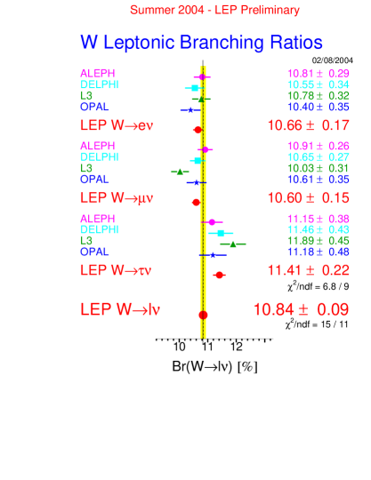
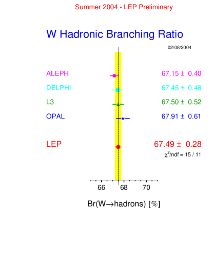
Figure 10.3: Leptonic and hadronic W branching fractions, as measured by the experiments, and the LEP combined values according to the procedures described in the text.

Within the Standard Model, the branching fractions of the W boson depend on the six matrix elements $|\mathrm{V}_{\mathrm{qq^{\prime}}}|$ of the Cabibbo–Kobayashi–Maskawa (CKM) quark mixing matrix not involving the top quark. In terms of these matrix elements, the leptonic branching fraction of the W boson $\mathcal{B}(\mbox{$\mathrm{W}\rightarrow\ell\overline{\nu}_{\ell}$})$ is given by

$$\frac{1}{\mathcal{B}(\mbox{$\mathrm{W}\rightarrow\ell\overline{\nu}_{\ell}$})}\quad=\quad 3\Bigg{\{}1+\bigg{[}1+\frac{\alpha_{s}(\mathrm{M}^{2}_{\mathrm{W}})}{\pi}\bigg{]}\sum_{\tiny\begin{array}[]{c}i=(u,c),\\ j=(d,s,b)\\ \end{array}}|\mathrm{V}_{ij}|^{2}\Bigg{\}},$$

where $\alpha_{s}(\mathrm{M}^{2}_{\mathrm{W}})$ is the strong coupling constant. Taking $\alpha_{s}(\mathrm{M}^{2}_{\mathrm{W}})=0.119\pm 0.002$ [145], and using the experimental knowledge of the sum $|\mathrm{V}_{ud}|^{2}+|\mathrm{V}_{us}|^{2}+|\mathrm{V}_{ub}|^{2}+|\mathrm{V}_{cd}|^{2}+|\mathrm{V}_{cb}|^{2}=1.0476\pm 0.0074$ [145], the above result can be interpreted as a measurement of $|\mathrm{V}_{cs}|$ which is the least well determined of these matrix elements:

$$|\mathrm{V}_{cs}|\quad=\quad 0.976\,\pm\,0.014.$$

The error includes a $\pm 0.0006$ contribution from the uncertainty on $\alpha_{s}$ and a $\pm 0.004$ contribution from the uncertainties on the other CKM matrix elements, the largest of which is that on $|\mathrm{V}_{cd}|$. These contributions are negligible in the error on this determination of $|\mathrm{V}_{cs}|$, which is dominated by the $\pm 0.013$ experimental error from the measurement of the W branching fractions. The value of $|\mathrm{V}_{cs}|$ is in agreement with unity.

10.4 Combination of the cos$\theta_{W^{-}}$ distribution

10.4.1 Introduction and definitions

In addition to measuring the total $\mathrm{W^{+}W^{-}}$ cross-section, the LEP experiments produce results for the differential cross-section, $\mathrm{d}(\sigma_{\mathrm{WW}})/\mathrm{d}(\mbox{$\cos\theta_{\mathrm{W}}$})$ ($\cos\theta_{\mathrm{W}}$ is the polar angle of the produced $\mathrm{W}^{-}$ with respect to the $\mathrm{e}^{-}$ beam direction). The LEP combination of these measurements will allow future theoretical models which predict deviations in this distribution to be tested against the LEP data in a direct and as much as possible model independent manner. To reconstruct the $\cos\theta_{\mathrm{W}}$ distribution it is necessary to identify the charges of the decaying W bosons. This can only be performed without significant ambiguity when one of W-boson decays via $\mathrm{W}\rightarrow e\nu$ or $\mathrm{W}\rightarrow\mu\nu$ (in which case the lepton provides the charge tag). Consequently, the combination of the differential cross-section measurements is performed for the $\mathrm{q\overline{q}}$e$\nu$ and $\mathrm{q\overline{q}}$$\mu\nu$ channels combined. Selected $\mathrm{q\overline{q}}$$\tau\nu$ events are not considered due to the larger backgrounds and difficulties in determining the tau lepton charge.

The measured $\mathrm{q\overline{q}}$e$\nu$ and $\mathrm{q\overline{q}}$$\mu\nu$ differential cross-sections are corrected to correspond to the CC03 set of diagrams with the additional constraint that the charged lepton is more than $20^{\circ}$ away from the $\mathrm{e}^{+}\mathrm{e}^{-}$ beam direction, $|\theta_{\ell^{\pm}}|>20^{\circ}$. This angular requirement corresponds closely to the experimental acceptance of the four LEP experiments and also greatly reduces the difference between the full $4f$ cross-section and the CC03 cross-section by reducing the contribution of $t$-channel diagrams in the $\mathrm{q\overline{q}}$e$\nu$ final state. The anlge $\cos\theta_{\mathrm{W}}$ is reconstructed from the four-momenta of the fermions from the ${\mathrm{W}^{-}}$ decay using the ECALO5 photon recombination scheme[127].

10.4.2 LEP combination method

The LEP combination is performed in ten bins of $\cos\theta_{\mathrm{W}}$. Because the differential cross-section distribution evolves with $\sqrt{s}$, reflecting the changing relative $s-$ and $t-$ channel contributions, the LEP data are divided into four $\sqrt{s}$ ranges: $180.0<\sqrt{s}\leq 184.0$; $184.0<\sqrt{s}\leq 194.0$; $194.0<\sqrt{s}\leq 204.0$; and $204.0<\sqrt{s}\leq 210.0$. It has been verified for each $\sqrt{s}$ range that the differences in the differential cross-sections at the mean value of $\sqrt{s}$ compared to the luminosity weighted sum of the differential cross-sections reflecting the actual distribution of the data across $\sqrt{s}$ are negligible compared to the statistical errors.

The experimental resolution in LEP on the reconstructed minus generated value of $\cos\theta_{\mathrm{W}}$ is typically 0.15-0.2 and, as a result, there is a significant migration between generated and reconstructed bins of $\cos\theta_{\mathrm{W}}$. The effects of bin-to-bin migration are not explicitely unfolded, instead each experiment obtains the cross-section in $i^{th}$ bin of the differential distribution, $\sigma_{i}$, from

$$\sigma_{i} = {{N_{i}-b_{i}}\over{\epsilon_{i}\cal{L}}},$$ (10.2)

where:

• is the observed number of $\mathrm{q\overline{q}}$e$\nu$/$\mathrm{q\overline{q}}$$\mu\nu$ events reconstructed in the $i$th bin of the $\cos\theta_{\mathrm{W}}$ distribution.

• is the expected number of background events in bin $i$. The contribution from four-fermion background is treated as in each of the experiments $\mathrm{W^{+}W^{-}}$ cross-section analyses.

• is the Monte Carlo efficiency in bin $i$, defined as $\epsilon_{i}=S_{i}/G_{i}$ where $S_{i}$ is the number of selected CC03 MC $\mathrm{q\overline{q}}$$\ell\overline{\nu}_{\ell}$ events reconstructed in bin $i$ and $G_{i}$ is the number of MC CC03 $\mathrm{q\overline{q}}$e$\nu$/$\mathrm{q\overline{q}}$$\mu\nu$ events with generated $\cos\theta_{\mathrm{W}}$ (calculated using the ECALO5 recombination scheme) lying in the $i$th bin ($|\theta_{\ell^{\pm}}|>20^{\circ}$). Selected $\mathrm{q\overline{q}}$$\tau\nu$ events are included in the numerator of the efficiency.

This bin-by-bin efficiency correction method has the advantages of simplicity and that the resulting $\sigma_{i}$ are uncorrelated. The main disadvantage of this procedure is that bin-by-bin migrations between generated and reconstructed $\cos\theta_{\mathrm{W}}$ are corrected purely on the basis of the Standard Model expectation. If the data deviate from it the resulting differential cross-section may be therefore biased toward the Standard Model expectation. However, the validity of the simple correction procedure has been tested by considering a range of deviations from the SM. Specifically the SM $\cos\theta_{\mathrm{W}}$ distribution was reweighted by $1+0.10\,(\mbox{$\cos\theta_{\mathrm{W}}$}-1.0)$, $1-0.20\,\mbox{$\cos^{2}\theta_{\mathrm{W}^{-}}$}$ , $1+0.20\,\mbox{$\cos^{2}\theta_{\mathrm{W}^{-}}$}$ and $1-0.40\,\mbox{$\cos^{8}\theta_{\mathrm{W}^{-}}$}$ and data samples generated corresponding to the combined LEP luminosity. These reweighting functions represent deviations which are large compared to the statistics of the combined LEP measurements. The bin-by-bin correction method was found to result in good $\chi^{2}$ distributions when the extracted $\cos\theta_{\mathrm{W}}$ distributions were compared with the underlying generated distribution (e.g. the worst case gave a mean $\chi^{2}$ of 11.3 for the 10 degrees of freedom corresponding to the ten $\cos\theta_{\mathrm{W}}$ bins).

For the LEP combination the systematic uncertainties on measured differential cross-sections are broken down into two terms: errors which are 100 % correlated between bins and experiments and errors which are correlated between bins but uncorrelated between experiments. This procedure reflects the the fact that the dominant systematic errors affect the overall normalisation of the measured distributions rather than the shape.

10.4.3 Results

For the Winter Conferences 2004 a first attempt of producing a LEP combination of the W angular distribution has been completed. It is based on final inputs from the DELPHI collaboration [131] and preliminary inputs from the L3 collaboration [132]. The detailed inputs by the experiments are reported in the appendix C, whereas Table 10.4 presents the combined LEP results according to the above described procedure. In the table the error breakdown bin by bin is also reported.

$\sqrt{s}$ interval (GeV)	Total luminosity (pb-1)	Lumi weighted $\sqrt{s}$ (GeV)
180-184	107.09	182.67

cos$\theta_{W-}$ bin $i$	1	2	3	4	5	6	7	8	9	10
$\sigma_{i}$ (pb)	0.701	0.714	0.819	1.137	1.414	2.171	2.765	2.651	4.317	5.276
$\delta\sigma_{i}$ (pb)	0.208	0.204	0.221	0.257	0.287	0.357	0.404	0.404	0.530	0.607
$\delta\sigma_{i}$(stat) (pb)	0.206	0.203	0.220	0.256	0.285	0.352	0.401	0.400	0.525	0.603
$\delta\sigma_{i}$(syst) (pb)	0.025	0.020	0.022	0.024	0.030	0.059	0.047	0.053	0.073	0.069

$\sqrt{s}$ interval (GeV)	Total luminosity (pb-1)	Lumi weighted $\sqrt{s}$ (GeV)
184-194	384.81	189.10

cos$\theta_{W-}$ bin $i$	1	2	3	4	5	6	7	8	9	10
$\sigma_{i}$ (pb)	0.792	0.847	1.067	1.148	1.406	1.507	1.889	2.758	4.371	5.731
$\delta\sigma_{i}$ (pb)	0.107	0.115	0.129	0.135	0.153	0.162	0.179	0.219	0.283	0.334
$\delta\sigma_{i}$(stat) (pb)	0.104	0.113	0.127	0.133	0.150	0.155	0.175	0.214	0.273	0.324
$\delta\sigma_{i}$(syst) (pb)	0.022	0.017	0.025	0.025	0.029	0.048	0.037	0.047	0.074	0.082

$\sqrt{s}$ interval (GeV)	Total luminosity (pb-1)	Lumi weighted $\sqrt{s}$ (GeV)
194-204	397.02	198.37

$\sigma_{i}$ (pb)	0.638	0.697	1.128	0.988	1.102	1.438	2.115	2.718	3.876	6.383
$\delta\sigma_{i}$ (pb)	0.089	0.099	0.124	0.122	0.131	0.153	0.184	0.209	0.262	0.342
$\delta\sigma_{i}$(stat) (pb)	0.088	0.098	0.123	0.120	0.129	0.146	0.181	0.205	0.252	0.331
$\delta\sigma_{i}$(syst) (pb)	0.016	0.014	0.020	0.022	0.024	0.045	0.034	0.041	0.070	0.086
cos$\theta_{W-}$ bin $i$	1	2	3	4	5	6	7	8	9	10

$\sqrt{s}$ interval (GeV)	Total luminosity (pb-1)	Lumi weighted $\sqrt{s}$ (GeV)
204-210	415.89	205.94

cos$\theta_{W-}$ bin $i$	1	2	3	4	5	6	7	8	9	10
$\sigma_{i}$ (pb)	0.568	0.582	0.685	0.996	1.328	1.486	1.995	2.779	4.612	7.585
$\delta\sigma_{i}$ (pb)	0.089	0.090	0.101	0.122	0.142	0.160	0.178	0.214	0.288	0.382
$\delta\sigma_{i}$(stat) (pb)	0.087	0.089	0.100	0.120	0.139	0.152	0.174	0.209	0.276	0.367
$\delta\sigma_{i}$(syst) (pb)	0.016	0.014	0.017	0.023	0.027	0.050	0.034	0.045	0.083	0.105

Table 10.4: Combined W^- differential angular cross-section in the 10 angular bins for the four chosen energy intervals. For each energy range, the sum of the measured integrated luminosities and the luminosity weighted centre-of-mass energy is reported. The results per angular bin in each of the energy interval are then presented: $\sigma_{i}$ indicates the average of d[$\sigma_{\mathrm{WW}}$(BR_eν+BR_μν)]/dcos$\theta_{\mathrm{W}^{-}}$ in the $i$-th bin of cos$\theta_{\mathrm{W}^{-}}$ with width 0.2. The values, in each bin, of the total, statistical and systematic errors are reported as well. All values are expressed in pb

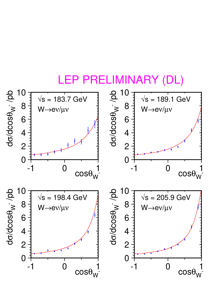
Figure 10.4: LEP combined d[$\sigma_{\mathrm{WW}}$(BR_eν+BR_μν)]/dcos$\theta_{\mathrm{W}^{-}}$ distributions for the four chosen energy intervals. The combined values (points) are superimposed with the four-fermion predictions from KandY [146].

The result is also presented in Figure 10.4, where the combined data are superimposed to the four-fermion theory predictions from KandY to guide the eye. The theory curve will soon be changed with one including only the CC03 component.

10.5 Single-W production cross-section

The LEP combination of the single-W production cross-section has been updated using the final ALEPH [147] and L3 [148, 149] results, and supersede the last combination presented at the 2003 Summer Conferences [126].

Single-W production at LEP2 is defined as the complete $t$-channel subset of Feynman diagrams contributing to e$\nu_{\mathrm{e}}$f$\bar{\mathrm{f}}^{\prime}$ final states, with additional cuts on kinematic variables to exclude the regions of phase space dominated by multiperipheral diagrams, where the cross-section calculation is affected by large uncertainties. The kinematic cuts used in the signal definitions are: $m_{\mathrm{q\overline{q}}}>45$ GeV/c² for the $\mathrm{e}\nu_{\mathrm{e}}\mathrm{q\overline{q}}$ final states, $E_{\ell}>20$ GeV for the $\mathrm{e}\nu_{\mathrm{e}}\mbox{$\ell\overline{\nu}_{\ell}$}$ final states with $\ell=\mu$ or $\tau$, and finally $|\cos\theta_{\mathrm{e^{-}}}|>0.95$, $|\cos\theta_{\mathrm{e^{+}}}|<0.95$ and $E_{\mathrm{e^{+}}}>20$ GeV (or the charge conjugate cuts) for the $\mathrm{e}\nu_{\mathrm{e}}\mathrm{e}\nu_{\mathrm{e}}$ final states.

In the LEP combination the correlation of the systematic errors in energy and among experiments is properly taken into account. The expected statistical errors have been used for all measurements, given the limited statistical precision of the single-W cross-section measurements.

The total and the hadronic single-W cross-sections, less contamined by $\gamma\gamma$ interaction contributions, are combined independently; the inputs by the four LEP experiments between 183 and 207 GeV are listed in Tables 10.5 and 10.6, and the corresponding LEP combined values presented.

$\sqrt{s}$	Single-W hadronic cross-section (pb)
(GeV)	ALEPH	DELPHI	L3	OPAL	LEP	$\chi^{2}/\textrm{d.o.f.}$
182.7	$0.44^{\phantom{0}+\phantom{0}0.29*}_{\phantom{0}-\phantom{0}0.24}\phantom{{}^{*}}$	—	$0.58^{\phantom{0}+\phantom{0}0.23\phantom{0}*}_{\phantom{0}-\phantom{0}0.20}$	—	$0.52\pm 0.17\phantom{{}^{*}}$	$\left\}\begin{array}[h]{rr}&\hbox{\multirowsetup 11.9/16}\\ &\\ &\\ &\\ &\\ &\\ &\\ &\\ \end{array}\right.$
188.6	$0.33^{\phantom{0}+\phantom{0}0.16*}_{\phantom{0}-\phantom{0}0.15}\phantom{{}^{*}}$	$0.44^{\phantom{0}+\phantom{0}0.28}_{\phantom{0}-\phantom{0}0.25}\phantom{{}^{*}}$	$0.52^{\phantom{0}+\phantom{0}0.14\phantom{0}*}_{\phantom{0}-\phantom{0}0.13}$	$0.53^{\phantom{0}+\phantom{0}0.14}_{\phantom{0}-\phantom{0}0.13}\phantom{{}^{*}}$	$0.46\pm 0.08\phantom{{}^{*}}$
191.6	$0.52^{\phantom{0}+\phantom{0}0.52*}_{\phantom{0}-\phantom{0}0.40}\phantom{{}^{*}}$	$0.01^{\phantom{0}+\phantom{0}0.19}_{\phantom{0}-\phantom{0}0.07}\phantom{{}^{*}}$	$0.84^{\phantom{0}+\phantom{0}0.44\phantom{0}*}_{\phantom{0}-\phantom{0}0.37}\phantom{{}^{*}}$	—	$0.54\pm 0.27\phantom{{}^{*}}$
195.5	$0.61^{\phantom{0}+\phantom{0}0.28*}_{\phantom{0}-\phantom{0}0.25}\phantom{{}^{*}}$	$0.78^{\phantom{0}+\phantom{0}0.38}_{\phantom{0}-\phantom{0}0.34}\phantom{{}^{*}}$	$0.66^{\phantom{0}+\phantom{0}0.25\phantom{0}*}_{\phantom{0}-\phantom{0}0.23}\phantom{{}^{*}}$	—	$0.66\pm 0.15\phantom{{}^{*}}$
199.5	$1.06^{\phantom{0}+\phantom{0}0.30*}_{\phantom{0}-\phantom{0}0.27}\phantom{{}^{*}}$	$0.16^{\phantom{0}+\phantom{0}0.29}_{\phantom{0}-\phantom{0}0.17}\phantom{{}^{*}}$	$0.37^{\phantom{0}+\phantom{0}0.22\phantom{0}*}_{\phantom{0}-\phantom{0}0.20}\phantom{{}^{*}}$	—	$0.55\pm 0.14\phantom{{}^{*}}$
201.6	$0.72^{\phantom{0}+\phantom{0}0.39*}_{\phantom{0}-\phantom{0}0.33}\phantom{{}^{*}}$	$0.55^{\phantom{0}+\phantom{0}0.47}_{\phantom{0}-\phantom{0}0.40}\phantom{{}^{*}}$	$1.10^{\phantom{0}+\phantom{0}0.40\phantom{0}*}_{\phantom{0}-\phantom{0}0.35}\phantom{{}^{*}}$	—	$0.81\pm 0.21\phantom{{}^{*}}$
204.9	$0.34^{\phantom{0}+\phantom{0}0.24*}_{\phantom{0}-\phantom{0}0.21}\phantom{{}^{*}}$	$0.50^{\phantom{0}+\phantom{0}0.35}_{\phantom{0}-\phantom{0}0.31}\phantom{{}^{*}}$	$0.42^{\phantom{0}+\phantom{0}0.25\phantom{0}*}_{\phantom{0}-\phantom{0}0.21}\phantom{{}^{*}}$	—	$0.40\pm 0.16\phantom{{}^{*}}$
206.6	$0.64^{\phantom{0}+\phantom{0}0.21*}_{\phantom{0}-\phantom{0}0.19}\phantom{{}^{*}}$	$0.37^{\phantom{0}+\phantom{0}0.24}_{\phantom{0}-\phantom{0}0.21}\phantom{{}^{*}}$	$0.66^{\phantom{0}+\phantom{0}0.20\phantom{0}*}_{\phantom{0}-\phantom{0}0.18}\phantom{{}^{*}}$	—	$0.58\pm 0.13\phantom{{}^{*}}$

Table 10.5: Single-W production cross-section from the four LEP experiments and combined values for the eight energies between 183 and 207 GeV, in the hadronic decay channel of the W boson. All results are preliminary with the exception of those indicated by ^∗.

$\sqrt{s}$	Single-W total cross-section (pb)
(GeV)	ALEPH	DELPHI	L3	OPAL	LEP	$\chi^{2}/\textrm{d.o.f.}$
182.7	$0.60^{\phantom{0}+\phantom{0}0.32*}_{\phantom{0}-\phantom{0}0.26}\phantom{{}^{*}}$	—	$0.80^{\phantom{0}+\phantom{0}0.28\phantom{0}*}_{\phantom{0}-\phantom{0}0.25}$	—	$0.70\pm 0.20\phantom{{}^{*}}$	$\left\}\begin{array}[h]{rr}&\hbox{\multirowsetup 11.1/16}\\ &\\ &\\ &\\ &\\ &\\ &\\ &\\ \end{array}\right.$
188.6	$0.55^{\phantom{0}+\phantom{0}0.18*}_{\phantom{0}-\phantom{0}0.16}\phantom{{}^{*}}$	$0.70^{\phantom{0}+\phantom{0}0.30}_{\phantom{0}-\phantom{0}0.26}\phantom{{}^{*}}$	$0.69^{\phantom{0}+\phantom{0}0.16\phantom{0}*}_{\phantom{0}-\phantom{0}0.15}$	$0.67^{\phantom{0}+\phantom{0}0.17}_{\phantom{0}-\phantom{0}0.15}\phantom{{}^{*}}$	$0.64\pm 0.09\phantom{{}^{*}}$
191.6	$0.89^{\phantom{0}+\phantom{0}0.58*}_{\phantom{0}-\phantom{0}0.44}\phantom{{}^{*}}$	$0.12^{\phantom{0}+\phantom{0}0.29}_{\phantom{0}-\phantom{0}0.14}\phantom{{}^{*}}$	$1.11^{\phantom{0}+\phantom{0}0.48\phantom{0}*}_{\phantom{0}-\phantom{0}0.41}\phantom{{}^{*}}$	—	$0.81\pm 0.30\phantom{{}^{*}}$
195.5	$0.87^{\phantom{0}+\phantom{0}0.31*}_{\phantom{0}-\phantom{0}0.27}\phantom{{}^{*}}$	$0.90^{\phantom{0}+\phantom{0}0.41}_{\phantom{0}-\phantom{0}0.36}\phantom{{}^{*}}$	$0.97^{\phantom{0}+\phantom{0}0.27\phantom{0}*}_{\phantom{0}-\phantom{0}0.25}\phantom{{}^{*}}$	—	$0.91\pm 0.17\phantom{{}^{*}}$
199.5	$1.31^{\phantom{0}+\phantom{0}0.32*}_{\phantom{0}-\phantom{0}0.29}\phantom{{}^{*}}$	$0.45^{\phantom{0}+\phantom{0}0.33}_{\phantom{0}-\phantom{0}0.20}\phantom{{}^{*}}$	$0.88^{\phantom{0}+\phantom{0}0.26\phantom{0}*}_{\phantom{0}-\phantom{0}0.24}\phantom{{}^{*}}$	—	$0.90\pm 0.16\phantom{{}^{*}}$
201.6	$0.80^{\phantom{0}+\phantom{0}0.42*}_{\phantom{0}-\phantom{0}0.35}\phantom{{}^{*}}$	$1.09^{\phantom{0}+\phantom{0}0.52}_{\phantom{0}-\phantom{0}0.43}\phantom{{}^{*}}$	$1.50^{\phantom{0}+\phantom{0}0.45\phantom{0}*}_{\phantom{0}-\phantom{0}0.40}\phantom{{}^{*}}$	—	$1.12\pm 0.23\phantom{{}^{*}}$
204.9	$0.65^{\phantom{0}+\phantom{0}0.27*}_{\phantom{0}-\phantom{0}0.23}\phantom{{}^{*}}$	$0.56^{\phantom{0}+\phantom{0}0.36}_{\phantom{0}-\phantom{0}0.30}\phantom{{}^{*}}$	$0.78^{\phantom{0}+\phantom{0}0.29\phantom{0}*}_{\phantom{0}-\phantom{0}0.25}\phantom{{}^{*}}$	—	$0.67\pm 0.18\phantom{{}^{*}}$
206.6	$0.81^{\phantom{0}+\phantom{0}0.22*}_{\phantom{0}-\phantom{0}0.20}\phantom{{}^{*}}$	$0.58^{\phantom{0}+\phantom{0}0.26}_{\phantom{0}-\phantom{0}0.23}\phantom{{}^{*}}$	$1.08^{\phantom{0}+\phantom{0}0.21\phantom{0}*}_{\phantom{0}-\phantom{0}0.20}\phantom{{}^{*}}$	—	$0.85\pm 0.14\phantom{{}^{*}}$

Table 10.6: Single-W total production cross-section from the four LEP experiments and combined values for the eight energies between 183 and 207 GeV. All results are preliminary with the exception of those indicated by ^∗.

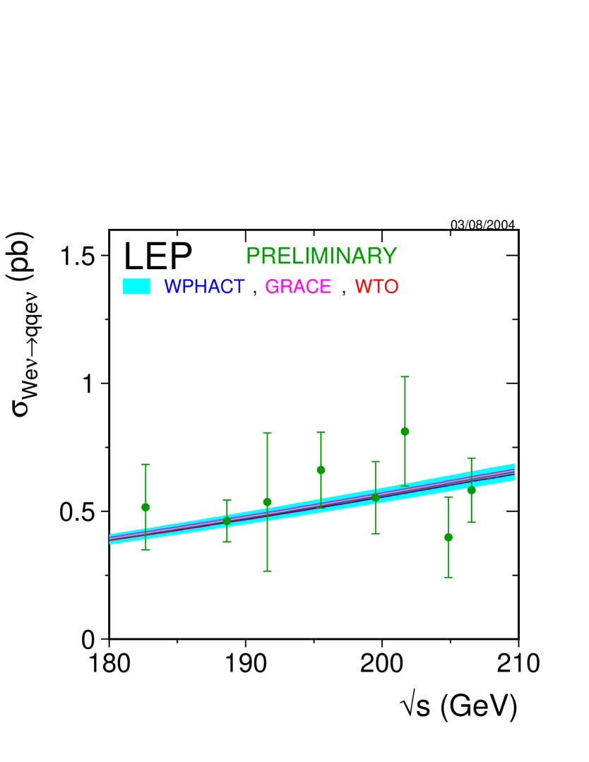
Figure 10.5: Measurements of the single-W production cross-section in the hadronic decay channel of the W boson, compared to the predictions of WTO [150], WPHACT [151] and grc4f [152] . The shaded area represents the $\pm 5$% uncertainty on the predictions.

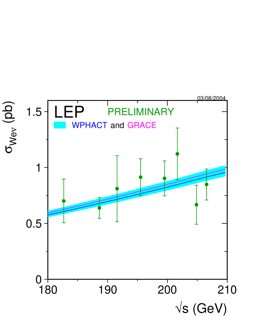
Figure 10.6: Measurements of the single-W total production cross-section, compared to the predictions of WPHACT  and grc4f. The shaded area represents the $\pm 5$% uncertainty on the predictions.

The LEP measurements of the single-W cross-section are shown, as a function of the LEP centre–of–mass energy, in Figure 10.5 for the hadronic decays and in Figure 10.6 for all decays of the W boson. In the two figures, the measurements are compared with the expected values from WPHACT [151] and grc4f [152]. WTO [150], which includes fermion-loop corrections for the hadronic final states, is also used in Figure 10.5. As discussed more in detail in [153] and [127], the theoretical predictions are scaled upward to correct for the implementation of QED radiative corrections at the wrong energy scale s. The full correction factor of 4%, derived [127] by the comparison to the theoretical predictions from SWAP [154], is conservatively taken as a systematic error. This uncertainty dominates the $\pm$5% theoretical error currently assigned to these predictions [153, 127], represented by the shaded area in Figures 10.5 and 10.6. All results, up to the highest centre–of–mass energies, are in agreement with the theoretical predictions.

The agreement can also be appreciated in Table 10.7, where the values of the ratio between measured and expected cross-section values according to the computations by grc4f and WPHACT  are reported. The combination is performed accounting for the energy and experiment correlations of the systematic sources. The results are also presented in Figure 10.7.

$\sqrt{s}$(GeV)	${\cal{R}}_{\mathrm{We\nu}}^{\footnotesize\mbox{\tt grc4f}}$	${\cal{R}}_{\mathrm{We\nu}}^{\footnotesize\mbox{WPHACT}}$
182.7	$1.121\pm 0.312$	$1.156\pm 0.322$
188.6	$0.913\pm 0.133$	$0.941\pm 0.137$
191.6	$1.099\pm 0.400$	$1.133\pm 0.412$
195.5	$1.156\pm 0.209$	$1.192\pm 0.216$
199.5	$1.071\pm 0.185$	$1.103\pm 0.190$
201.6	$1.286\pm 0.265$	$1.325\pm 0.273$
204.9	$0.726\pm 0.191$	$0.748\pm 0.196$
206.6	$0.901\pm 0.147$	$0.923\pm 0.152$
$\chi^{2}$/d.o.f	11.1/16	11.1/16
Average	$0.973\pm 0.073$	$1.002\pm 0.075$
$\chi^{2}$/d.o.f	16.0/23	16.1/23

Table 10.7: Ratios of LEP combined total single-W cross-section measurements to the expectations according to grc4f [152] and WPHACT [151]. The resulting averages over energies are also given. The averages take into account inter-experiment as well as inter-energy correlations of systematic errors.

      

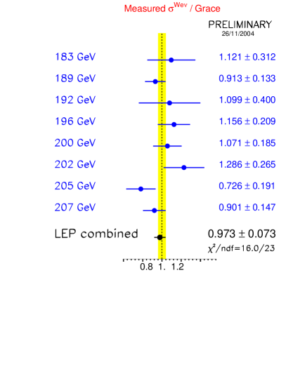
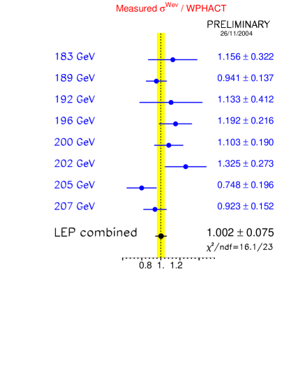
Figure 10.7: Ratios of LEP combined total single-W cross-section measurements to the expectations according to grc4f [152] and WPHACT [151]. The yellow bands represent constant relative errors of 5% on the two cross-section predictions.

The theory predictions and the details of the experimental inputs and the LEP combined values of the single-W cross-sections and the ratios to theory are reported in Appendix C.

10.6 Z-pair production cross-section

The Z-pair production cross-section is defined as the NC02 [127] contribution to four-fermion cross-section. Final results from DELPHI, L3 and OPAL at all centre–of–mass energies are available [155, 156, 157]. ALEPH published final results at 183 and 189 GeV [158] and contributed preliminary results for all other energies up to 207 GeV [159].

$\sqrt{s}$	ZZ cross-section (pb)
(GeV)	ALEPH	DELPHI	L3	OPAL	LEP	$\chi^{2}/\textrm{d.o.f.}$
182.7	$0.11^{\phantom{0}+\phantom{0}0.16\phantom{0}*}_{\phantom{0}-\phantom{0}0.12}$	$0.35^{\phantom{0}+\phantom{0}0.20\phantom{0}*}_{\phantom{0}-\phantom{0}0.15}$	$0.31\pm 0.17^{*}$	$0.12^{\phantom{0}+\phantom{0}0.20\phantom{0}*}_{\phantom{0}-\phantom{0}0.18}$	$0.22\pm 0.08\phantom{{}^{*}}^{*}$	$\left\}\begin{array}[h]{rr}&\hbox{\multirowsetup 16.1/24}\\ &\\ &\\ &\\ &\\ &\\ &\\ &\\ \end{array}\right.$
188.6	$0.67^{\phantom{0}+\phantom{0}0.14\phantom{0}*}_{\phantom{0}-\phantom{0}0.13}$	$0.52^{\phantom{0}+\phantom{0}0.12\phantom{0}*}_{\phantom{0}-\phantom{0}0.11}$	$0.73\pm 0.15\phantom{{}^{*}}^{*}$	$0.80^{\phantom{0}+\phantom{0}0.15\phantom{0}*}_{\phantom{0}-\phantom{0}0.14}$	$0.66\pm 0.07\phantom{{}^{*}}^{*}$
191.6	$0.53^{\phantom{0}+\phantom{0}0.34}_{\phantom{0}-\phantom{0}0.27}\phantom{{}^{0*}}$	$0.63^{\phantom{0}+\phantom{0}0.36*}_{\phantom{0}-\phantom{0}0.30}\phantom{{}^{0*}}$	$0.29\pm 0.22^{*}$	$1.29^{\phantom{0}+\phantom{0}0.48*}_{\phantom{0}-\phantom{0}0.41}\phantom{{}^{0*}}$	$0.65\pm 0.17\phantom{{}^{*}}$
195.5	$0.69^{\phantom{0}+\phantom{0}0.23}_{\phantom{0}-\phantom{0}0.20}\phantom{{}^{0*}}$	$1.05^{\phantom{0}+\phantom{0}0.25*}_{\phantom{0}-\phantom{0}0.22}\phantom{{}^{0*}}$	$1.18\pm 0.26^{*}$	$1.13^{\phantom{0}+\phantom{0}0.27*}_{\phantom{0}-\phantom{0}0.25}\phantom{{}^{0*}}$	$0.99\pm 0.12\phantom{{}^{*}}$
199.5	$0.70^{\phantom{0}+\phantom{0}0.22}_{\phantom{0}-\phantom{0}0.20}\phantom{{}^{0*}}$	$0.75^{\phantom{0}+\phantom{0}0.20*}_{\phantom{0}-\phantom{0}0.18}\phantom{{}^{0*}}$	$1.25\pm 0.27^{*}$	$1.05^{\phantom{0}+\phantom{0}0.26*}_{\phantom{0}-\phantom{0}0.23}\phantom{{}^{0*}}$	$0.90\pm 0.12\phantom{{}^{*}}$
201.6	$0.70^{\phantom{0}+\phantom{0}0.33}_{\phantom{0}-\phantom{0}0.28}\phantom{{}^{0*}}$	$0.85^{\phantom{0}+\phantom{0}0.33*}_{\phantom{0}-\phantom{0}0.28}\phantom{{}^{0*}}$	$0.95\pm 0.39^{*}$	$0.79^{\phantom{0}+\phantom{0}0.36*}_{\phantom{0}-\phantom{0}0.30}\phantom{{}^{0*}}$	$0.81\pm 0.17\phantom{{}^{*}}$
204.9	$1.21^{\phantom{0}+\phantom{0}0.26}_{\phantom{0}-\phantom{0}0.23}\phantom{{}^{0*}}$	$1.03^{\phantom{0}+\phantom{0}0.23*}_{\phantom{0}-\phantom{0}0.20}\phantom{{}^{0*}}$	$0.77^{\phantom{0}+\phantom{0}0.21*}_{\phantom{0}-\phantom{0}0.19}\phantom{{}^{0*}}$	$1.07^{\phantom{0}+\phantom{0}0.28*}_{\phantom{0}-\phantom{0}0.25}\phantom{{}^{0*}}$	$0.98\pm 0.13\phantom{{}^{*}}$
206.6	$1.01^{\phantom{0}+\phantom{0}0.19}_{\phantom{0}-\phantom{0}0.17}\phantom{{}^{0*}}$	$0.96^{\phantom{0}+\phantom{0}0.16*}_{\phantom{0}-\phantom{0}0.15}\phantom{{}^{0*}}$	$1.09^{\phantom{0}+\phantom{0}0.18*}_{\phantom{0}-\phantom{0}0.17}\phantom{{}^{0*}}$	$0.97^{\phantom{0}+\phantom{0}0.20*}_{\phantom{0}-\phantom{0}0.19}\phantom{{}^{0*}}$	$0.99\pm 0.09\phantom{{}^{*}}$

Table 10.8: Z-pair production cross-sections from the four LEP experiments and combined values for the eight energies between 183 and 207 GeV. All results are preliminary with the exception of those indicated by ^∗.

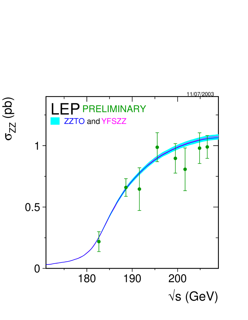
Figure 10.8: Measurements of the Z-pair production cross-section, compared to the predictions of YFSZZ [160] and ZZTO [161]. The shaded area represent the $\pm 2$% uncertainty on the predictions.

$\sqrt{s}$(GeV)	${\cal{R}}_{\mathrm{ZZ}}^{\footnotesize\mbox{ZZTO}}$	${\cal{R}}_{\mathrm{ZZ}}^{\footnotesize\mbox{YFSZZ}}$
182.7	$0.857\pm 0.320$	$0.857\pm 0.320$
188.6	$1.017\pm 0.113$	$1.007\pm 0.111$
191.6	$0.831\pm 0.225$	$0.826\pm 0.224$
195.5	$1.100\pm 0.133$	$1.100\pm 0.133$
199.5	$0.915\pm 0.125$	$0.912\pm 0.124$
201.6	$0.799\pm 0.174$	$0.795\pm 0.173$
204.9	$0.937\pm 0.121$	$0.931\pm 0.120$
206.6	$0.937\pm 0.091$	$0.928\pm 0.090$
$\chi^{2}$/d.o.f	16.1/24	16.1/24
Average	$0.952\pm 0.052$	$0.945\pm 0.052$
$\chi^{2}$/d.o.f	19.1/31	19.1/31

Table 10.9: Ratios of LEP combined Z-pair cross-section measurements to the expectations according to ZZTO [161] and YFSZZ [160]. The results of the combined fits are given in the table together with the resulting $\chi^{2}$. Both fits take into account inter-experiment as well as inter-energy correlations of systematic errors.

      

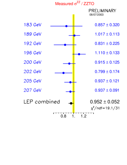
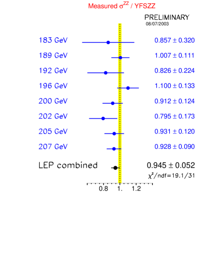
Figure 10.9: Ratios of LEP combined Z-pair cross-section measurements to the expectations according to ZZTO [161] and YFSZZ [160] The yellow bands represent constant relative errors of 2% on the two cross-section predictions.

The combination of results is performed with the same technique used for the WW cross-section. The symmetrized expected statistical error of each analysis is used, to avoid biases due to the limited number of selected events. All the cross-sections used for the combination and presented in Table 10.8 are determined by the experiments using the frequentist approach, i.e. without assuming any prior for the value of the cross-section itself.

The measurements are shown in Figure 10.8 as a function of the LEP centre–of–mass energy, where they are compared to the YFSZZ [160] and ZZTO [161] predictions. Both these calculations have an estimated uncertainty of $\pm 2\%$ [127]. The data do not show any significant deviation from the theoretical expectations.

In analogy with the W-pair cross-section, a value for ${\cal{R}}_{\mathrm{ZZ}}$ can also be determined: its definition and the procedure of the combination follows the one described for ${\cal{R}}_{\mathrm{WW}}$. The data are compared with the YFSZZ and ZZTO predictions; Table 10.9 reports the numerical values of ${\cal{R}}_{\mathrm{ZZ}}$ in energy and combined, whereas figure 10.9 show them in comparison to unity, where the $\pm$2% error on the theoretical ZZ cross-section is shown as a yellow band. The experimental accuracy on the combined value of ${\cal{R}}_{\mathrm{ZZ}}$ is about 5%.

The theory predictions, the details of the experimental inputs with the the breakdown of the error contributions and the LEP combined values of the total cross-sections and the ratios to theory are reported in Appendix C.

10.7 Single-Z production cross-section

Single-Z production at LEP2 is studied considering only the $eeq\bar{q}$, $ee\mu\mu$ final states with the following phase space cuts and assuming one visible electron: $m_{q\bar{q}}(m_{\mu\mu})>60$ GeV/c², $\theta_{\mathrm{e^{+}}}<12$ degrees, 12 degrees$<\theta_{\mathrm{e^{-}}}<$120 degrees and $E_{\mathrm{e^{-}}}>$3 GeV, with obvious notation and where the angle is defined with respect to the beam pipe, with the positron direction being along $+z$ and the electron direction being along $-z$. Corresponding cuts are imposed when the positron is visible: $\theta_{\mathrm{e^{-}}}>168$ degrees, 60 degrees$<\theta_{\mathrm{e^{+}}}<$168 degrees and $E_{\mathrm{e^{+}}}>$3 GeV.

The LEP combination of the single-Z production cross-section uses final results by the ALEPH [147] and the L3 [162] Collaborations and preliminary results from DELPHI [163]. The results concern the hadronic and the leptonic channel and all the centre–of–mass energies from 183 to 209 GeV. The combination was updated with respect to the Summer 2003 Conferences because of the final ALEPH input.

$\sqrt{s}$	Single-Z hadronic cross-section (pb)
(GeV)	ALEPH	DELPHI	L3	OPAL	LEP	$\chi^{2}/\textrm{d.o.f.}$
182.7	$0.27^{\phantom{0}+\phantom{0}0.21\phantom{0}*}_{\phantom{0}-\phantom{0}0.16}$	$0.56^{\phantom{0}+\phantom{0}0.27\phantom{0}}_{\phantom{0}-\phantom{0}0.23}$	$0.51^{\phantom{0}+\phantom{0}0.19\phantom{0}*}_{\phantom{0}-\phantom{0}0.16}$	—	$0.45\pm 0.11\phantom{{}^{*}}$	$\left\}\begin{array}[h]{rr}&\hbox{\multirowsetup 12.9/16}\\ &\\ &\\ &\\ &\\ &\\ &\\ &\\ \end{array}\right.$
188.6	$0.42^{\phantom{0}+\phantom{0}0.14*}_{\phantom{0}-\phantom{0}0.12}\phantom{{}^{*}}$	$0.65^{\phantom{0}+\phantom{0}0.16}_{\phantom{0}-\phantom{0}0.14}\phantom{{}^{*}}$	$0.55^{\phantom{0}+\phantom{0}0.11\phantom{0}*}_{\phantom{0}-\phantom{0}0.10}$	—	$0.53\pm 0.07\phantom{{}^{*}}$
191.6	$0.61^{\phantom{0}+\phantom{0}0.39*}_{\phantom{0}-\phantom{0}0.29}\phantom{{}^{*}}$	$0.63^{\phantom{0}+\phantom{0}0.40}_{\phantom{0}-\phantom{0}0.30}\phantom{{}^{*}}$	$0.60^{\phantom{0}+\phantom{0}0.26*}_{\phantom{0}-\phantom{0}0.21}\phantom{{}^{*}}$	—	$0.61\pm 0.15\phantom{{}^{*}}$
195.5	$0.72^{\phantom{0}+\phantom{0}0.24*}_{\phantom{0}-\phantom{0}0.20}\phantom{{}^{*}}$	$0.66^{\phantom{0}+\phantom{0}0.22}_{\phantom{0}-\phantom{0}0.19}\phantom{{}^{*}}$	$0.40^{\phantom{0}+\phantom{0}0.13*}_{\phantom{0}-\phantom{0}0.11}\phantom{{}^{*}}$	—	$0.55\pm 0.09\phantom{{}^{*}}$
199.5	$0.60^{\phantom{0}+\phantom{0}0.21*}_{\phantom{0}-\phantom{0}0.18}\phantom{{}^{*}}$	$0.57^{\phantom{0}+\phantom{0}0.20}_{\phantom{0}-\phantom{0}0.17}\phantom{{}^{*}}$	$0.33^{\phantom{0}+\phantom{0}0.13*}_{\phantom{0}-\phantom{0}0.11}\phantom{{}^{*}}$	—	$0.47\pm 0.10\phantom{{}^{*}}$
201.6	$0.89^{\phantom{0}+\phantom{0}0.35*}_{\phantom{0}-\phantom{0}0.28}\phantom{{}^{*}}$	$0.19^{\phantom{0}+\phantom{0}0.21}_{\phantom{0}-\phantom{0}0.16}\phantom{{}^{*}}$	$0.81^{\phantom{0}+\phantom{0}0.27*}_{\phantom{0}-\phantom{0}0.23}\phantom{{}^{*}}$	—	$0.67\pm 0.13\phantom{{}^{*}}$
204.9	$0.42^{\phantom{0}+\phantom{0}0.17*}_{\phantom{0}-\phantom{0}0.15}\phantom{{}^{*}}$	$0.37^{\phantom{0}+\phantom{0}0.18}_{\phantom{0}-\phantom{0}0.15}\phantom{{}^{*}}$	$0.56^{\phantom{0}+\phantom{0}0.16*}_{\phantom{0}-\phantom{0}0.14}\phantom{{}^{*}}$	—	$0.47\pm 0.10\phantom{{}^{*}}$
206.6	$0.70^{\phantom{0}+\phantom{0}0.17*}_{\phantom{0}-\phantom{0}0.15}\phantom{{}^{*}}$	$0.68^{\phantom{0}+\phantom{0}0.16}_{\phantom{0}-\phantom{0}0.14}\phantom{{}^{*}}$	$0.59^{\phantom{0}+\phantom{0}0.12*}_{\phantom{0}-\phantom{0}0.11}\phantom{{}^{*}}$	—	$0.65\pm 0.07\phantom{{}^{*}}$

Table 10.10: Single-Z hadronic production cross-section from the four LEP experiments and combined values for the eight energies between 183 and 207 GeV. All results are preliminary with the exception of those indicated by ^∗.

	Single-Z cross-section into muons(pb)
	ALEPH	DELPHI	L3	OPAL	LEP
Av. $\sqrt{s}$(GeV)	196.67	197.10	196.60	—	196.79
$\sigma_{Zee\rightarrow\mu\mu ee}$	$0.055\pm 0.016\phantom{{}^{*}}^{*}$	$0.070^{\phantom{0}+\phantom{0}0.023\phantom{0}}_{\phantom{0}-\phantom{0}0.019}$	$0.043\pm 0.013\phantom{{}^{*}}^{*}$	—	$0.057\pm 0.009\phantom{{}^{*}}$

Table 10.11: Preliminary energy averaged single-Z production cross-section into muons from the four LEP experiments and combined values. The results indicated with ^∗ are final.

Tables 10.10 and 10.11 synthesize the inputs by the experiments and the corresponding LEP combinations in the hadronic and muon channel, respectively. The $ee\mu\mu$ cross-section is already combined in energy by the individual experiments to increase the statistics of the data. The combination accounts for energy and experiment correlation of the systematic errors. The results in the hadronic channel are compared with the WPHACT and grc4f predictions as a function of the centre–of–mass energy and shown in figure 10.10. Table 10.12 and figure 10.11 show the preliminary values of the ratio between measured and expected cross-sections at the various energy points and the combined value; the testing accuracy of the combined value is about 7% with three experiments contributing in the average.

The detailed breakdown of the inputs of the experiments with the split up of the systematic contribution according to the correlations for the single-Z cross-section and its ratio to theory can be found in Appendix C.

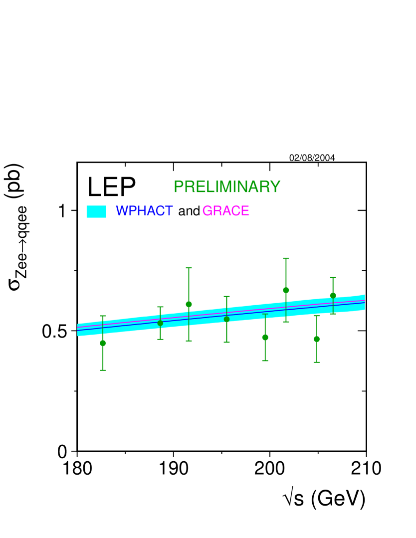
Figure 10.10: Measurements of the single-Z hadronic production cross-section, compared to the predictions of WPHACT and grc4f. The shaded area represents the $\pm 5$% uncertainty on the predictions.

$\sqrt{s}$(GeV)	${\cal{R}}_{\mathrm{Zee}}^{\footnotesize\mbox{\tt grc4f}}$	${\cal{R}}_{\mathrm{Zee}}^{\footnotesize\mbox{WPHACT}}$
182.7	$0.870\pm 0.219$	$0.875\pm 0.220$
188.6	$0.983\pm 0.126$	$0.990\pm 0.127$
191.6	$1.104\pm 0.276$	$1.112\pm 0.278$
195.5	$0.963\pm 0.167$	$0.971\pm 0.169$
199.5	$0.809\pm 0.165$	$0.816\pm 0.167$
201.6	$1.129\pm 0.223$	$1.139\pm 0.224$
204.9	$0.770\pm 0.161$	$0.777\pm 0.162$
206.6	$1.061\pm 0.124$	$1.067\pm 0.125$
$\chi^{2}$/d.o.f	12.2/16	12.2/16
Average	$0.955\pm 0.065$	$0.963\pm 0.065$
$\chi^{2}$/d.o.f	17.0/23	16.9/23

Table 10.12: Ratios of LEP combined single-Z hadronic cross-section measurements to the expectations according to grc4f [152] and WPHACT [151]. The resulting averages over energies are also given. The averages take into account inter-experiment as well as inter-energy correlations of systematic errors.

      

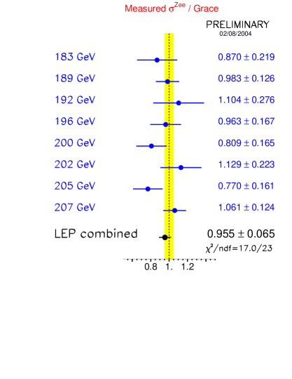
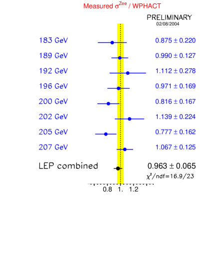
Figure 10.11: Ratios of LEP combined single-Z hadronic cross-section measurements to the expectations according to grc4f [152] and WPHACT [151]. The yellow bands represent constant relative errors of 5% on the two cross-section predictions.

10.8 WW$\gamma$ production cross-section

A LEP combination of the WW$\gamma$ production cross-section has been performed using final DELPHI [164], L3 [165] and OPAL [166] inputs to the Summer 2003 Conferences. The signal is defined as the part of the WW$\gamma$ process with the following cuts to the photon: $E_{\gamma}>$5 GeV, $|\cos\theta_{\gamma}|<$0.95, $|\cos\theta_{\gamma,f}|<$0.90 and $m_{W}-2\Gamma_{W}<m_{ff^{\prime}}<m_{W}+2\Gamma_{W}$ where $\theta_{\gamma,f}$ is the angle between the photon and the closest charged fermion and $m_{ff^{\prime}}$ is the invariant mass of fermions from the Ws.

In order to increase the statistics the LEP combination is performed in energy intervals rather than at each energy point; they are defined according to the LEP2 running period where more statistics was accumulated. The luminosity weighted centre–of–mass per interval is determined in each experiment and then combined to obtain the corresponding value in the combination. Table 10.13 reports those energies and the cross-sections measured by the experiments, together with the combined LEP values.

$\sqrt{s}$	WW$\gamma$ cross-section (pb)
(GeV)	ALEPH	DELPHI	L3	OPAL	LEP
188.6	—	$0.05\pm 0.08\phantom{{}^{*}}$	$0.20\pm 0.09\phantom{{}^{*}}$	$0.16\pm 0.04\phantom{{}^{*}}$	$0.15\pm 0.03\phantom{{}^{*}}$
194.4	—	$0.17\pm 0.12\phantom{{}^{*}}$	$0.17\pm 0.10\phantom{{}^{*}}$	$0.17\pm 0.06\phantom{{}^{*}}$	$0.17\pm 0.05\phantom{{}^{*}}$
200.2	—	$0.34\pm 0.12\phantom{{}^{*}}$	$0.43\pm 0.13\phantom{{}^{*}}$	$0.21\pm 0.06\phantom{{}^{*}}$	$0.27\pm 0.05\phantom{{}^{*}}$
206.1	—	$0.18\pm 0.08\phantom{{}^{*}}$	$0.13\pm 0.08\phantom{{}^{*}}$	$0.30\pm 0.05\phantom{{}^{*}}$	$0.24\pm 0.04\phantom{{}^{*}}$

Table 10.13: WW$\gamma$ production cross-section from the four LEP experiments and combined values for the four energy bins. All results are final.

Figure 10.12 shows the combined data points compared with the cross-section prediction by EEWWG [167] and by RACOONWW. The RACOONWW is shown in the figure without any theory error band.

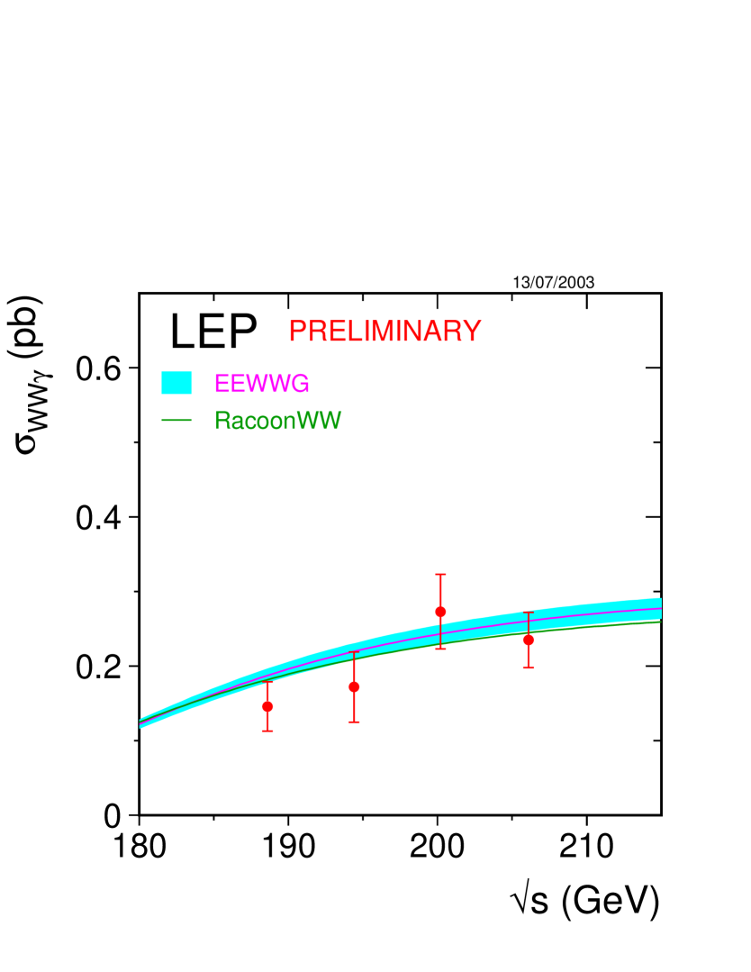
Figure 10.12: Measurements of the WW$\gamma$ production cross-section, compared to the predictions of EEWWG [167] and RACOONWW [140]. The shaded area in the EEWWG curve represents the $\pm 5$% uncertainty on the predictions.

10.9 Summary

The updated LEP combinations of the W-pair and single boson production cross-section, together with the first attempt to combine W angular distributions, have been presented. The combinations are based on data collected up to 209 GeV by the four LEP experiments.

All measurements agree with the expectations. In the fit to the W branching fractions without the assumption of lepton universality an excess of the W branching ratio into $\tau\nu_{\tau}$ with respect to the other lapton families is observed in the data. This excess is above two standard deviations from both the branching ratio into $e\nu_{e}$ and into $\mu\nu_{\mu}$.

This note still reflects a preliminary status of the analyses at the time of the Summer 2004 Conferences. A definitive statement on these results and the ones not updated for these Conferences must wait for publication by each collaboration. Further work on the possibility of providing a LEP combination of other cross-sections in the neutral current sector (Z$\gamma^{*}$, Z$\gamma\gamma$) are ongoing.

Chapter 11 Electroweak Gauge Boson Self Couplings

Updates with respect to summer 2003:
Unchanged w.r.t. summer 2003: Results are preliminary.

11.1 Introduction

The measurement of gauge boson couplings and the search for possible anomalous contributions due to the effects of new physics beyond the Standard Model are among the principal physics aims at LEP-II [168]. Combined preliminary measurements of triple gauge boson couplings are presented here. Results from W-pair production are combined in single and two-parameter fits, including updated results from ALEPH, L3 and OPAL as well as an improved treatment of the main systematic effect in our previous combination, the uncertainty in the $O(\alpha_{em})$ correction. An updated combination of quartic gauge coupling (QGC) results for the $\mathrm{ZZ}\gamma\gamma$  vertex is also presented, including data from ALEPH, L3 and OPAL. The combination of QGCs associated with the $\mathrm{WW}\gamma\gamma$ vertex, including the sign convention as reported in [169, 170] and the reweighting based on [169] is foreseen for our next report. The combination of neutral TGCs measured in ZZ production (f-couplings) has been updated, including new results from L3 and OPAL. The combinations for neutral TGCs accessible through ${\rm Z}\gamma$ production (h-couplings) reported in 2001 still remain valid  [171].

The W-pair production process, $\mathrm{e^{+}e^{-}\rightarrow\mathrm{W^{+}W^{-}}}$, involves charged triple gauge boson vertices between the $\mathrm{W^{+}W^{-}}$ and the Z or photon. During LEP-II operation, about 10,000 W-pair events were collected by each experiment. Single W ($\mathrm{e}\nu\mathrm{W}$) and single photon ($\nu\bar{\nu}\gamma$) production at LEP are also sensitive to the $\mathrm{WW}\gamma$ vertex. Results from these channels are also included in the combination for some experiments; the individual references should be consulted for details.

For the charged TGCs, Monte Carlo calculations (RacoonWW [172] and YFSWW [173]) incorporating an improved treatment of $O(\alpha_{em})$ corrections to the WW production have become our standard by now. The corrections affect the measurements of the charged TGCs in W-pair production. Results, some of them preliminary, including these $O(\alpha_{em})$ corrections have been submitted from all four LEP collaborations ALEPH [174], DELPHI [175], L3 [176] and OPAL [177]. LEP combinations are made for the charged TGC measurements in single- and two-parameter fits.

At centre-of-mass energies exceeding twice the Z boson mass, pair production of Z bosons is kinematically allowed. Here, one searches for the possible existence of triple vertices involving only neutral electroweak gauge bosons. Such vertices could also contribute to Z$\gamma$ production. In contrast to triple gauge boson vertices with two charged gauge bosons, purely neutral gauge boson vertices do not occur in the Standard Model of electroweak interactions.

Within the Standard Model, quartic electroweak gauge boson vertices with at least two charged gauge bosons exist. In $\mathrm{e}^{+}\mathrm{e}^{-}$ collisions at LEP-II centre-of-mass energies, the ${\mathrm{WWZ}\gamma}$ and $\mathrm{WW}\gamma\gamma$ vertices contribute to $\mathrm{WW}\gamma$ and $\nu\bar{\nu}\gamma\gamma$ production in $s$-channel and $t$-channel, respectively. The effect of the Standard Model quartic electroweak vertices is below the sensitivity of LEP-II. Quartic gauge boson vertices with only neutral bosons, like the $\mathrm{ZZ}\gamma\gamma$  vertex, do not exist in the Standard Model. However, anomalous QGCs associated with this vertex are studied at LEP.

Anomalous quartic vertices are searched for in the production of $\mathrm{WW}\gamma$, $\nu\bar{\nu}\gamma\gamma$ and $\mathrm{Z}\gamma\gamma$ final states. The couplings related to the $\mathrm{ZZ}\gamma\gamma$  and $\mathrm{WW}\gamma\gamma$ vertices are assumed to be different [178], and are therefore treated separately. In this report, we only combine the results for the anomalous couplings associated with the $\mathrm{ZZ}\gamma\gamma$  vertex. The combination of the $\mathrm{WW}\gamma\gamma$ vertex couplings is foreseen for the near future.

11.1.1 Charged Triple Gauge Boson Couplings

The parametrisation of the charged triple gauge boson vertices is described in References [179, 180, 181, 182, 183, 184, 168]. The most general Lorentz invariant Lagrangian which describes the triple gauge boson interaction has fourteen independent complex couplings, seven describing the WW$\gamma$ vertex and seven describing the WWZ vertex. Assuming electromagnetic gauge invariance as well as C and P conservation, the number of independent TGCs reduces to five. A common set is {$\mbox{$g_{1}^{\mathrm{Z}}$},\mbox{$\kappa_{\mathrm{Z}}$},\mbox{$\kappa_{\gamma}$},\mbox{$\lambda_{\mathrm{Z}}$}$, $\lambda_{\gamma}$} where $\mbox{$g_{1}^{\mathrm{Z}}$}=\mbox{$\kappa_{\mathrm{Z}}$}=\mbox{$\kappa_{\gamma}$}=1$ and $\mbox{$\lambda_{\mathrm{Z}}$}=\mbox{$\lambda_{\gamma}$}=0$ in the Standard Model. The parameters proposed in [168] and used by the LEP experiments are $g_{1}^{\mathrm{Z}}$, $\lambda_{\gamma}$ and $\kappa_{\gamma}$ with the gauge constraints:

$$\kappa_{\mathrm{Z}} = \mbox{$g_{1}^{\mathrm{Z}}$}-(\mbox{$\kappa_{\gamma}$}-1)\tan^{2}\theta_{\mathrm{W}}\,,$$ (11.1)

$$\lambda_{\mathrm{Z}} = \mbox{$\lambda_{\gamma}$}\,,$$ (11.2)

where $\theta_{W}$ is the weak mixing angle. The couplings are considered as real, with the imaginary parts fixed to zero. In contrast to previous LEP combinations [185, 171], we are quoting the measured coupling values themselves and not their deviation from the Standard Model.

Note that the photonic couplings $\lambda_{\gamma}$ and $\kappa_{\gamma}$ are related to the magnetic and electric properties of the W-boson. One can write the lowest order terms for a multipole expansion describing the W-$\gamma$ interaction as a function of $\lambda_{\gamma}$ and $\kappa_{\gamma}$. For the magnetic dipole moment $\mu_{W}$ and the electric quadrupole moment $q_{W}$ one obtains $e(1+\kappa_{\gamma}+\lambda_{\gamma})/2m_{\mathrm{W}}$ and $-e(\kappa_{\gamma}-\lambda_{\gamma})/m_{\mathrm{W}}^{2}$, respectively.

The inclusion of $O(\alpha_{em})$ corrections in the Monte Carlo calculations has a considerable effect on the charged TGC measurement. Both the total cross-section and the differential distributions are affected. The cross-section is reduced by 1-2% (depending on the energy). Amongst the differential distributions, the effects are naturally more complex. The polar W^- production angle carries most of the information on the TGC parameters; its shape is modified to be more forwardly peaked. In a fit to data, the $O(\alpha_{em})$ effect manifests itself as a negative shift of the obtained TGC values with a magnitude of typically -0.015 for $\lambda_{\gamma}$ and $g_{1}^{\mathrm{Z}}$  and -0.04 for $\kappa_{\gamma}$.

11.1.2 Neutral Triple Gauge Boson Couplings

There are two classes of Lorentz invariant structures associated with neutral TGC vertices which preserve $U(1)_{em}$ and Bose symmetry, as described in [180, 186].

The first class refers to anomalous Z$\gamma\gamma^{*}$ and $\rm Z\gamma\rm Z^{*}$ couplings which are accessible at LEP in the process $\mathrm{e^{+}e^{-}}\rightarrow{\rm Z}\gamma$. The parametrisation contains eight couplings: $h_{i}^{V}$ with $i=1,...,4$ and $V=\gamma$,Z. The superscript $\gamma$ refers to Z$\gamma\gamma^{*}$ couplings and superscript Z refers to $\rm Z\gamma\rm Z^{*}$ couplings. The photon and the Z boson in the final state are considered as on-shell particles, while the third boson at the vertex, the $s$-channel internal propagator, is off shell. The couplings $h_{1}^{V}$ and $h_{2}^{V}$ are CP-odd while $h_{3}^{V}$ and $h_{4}^{V}$ are CP-even.

The second class refers to anomalous $\rm{ZZ}\gamma^{*}$ and $\rm{ZZZ}^{*}$ couplings which are accessible at LEP-II in the process $\mathrm{e^{+}e^{-}}\rightarrow$ ZZ. This anomalous vertex is parametrised in terms of four couplings: $f_{i}^{V}$ with $i=4,5$ and $V=\gamma$,Z. The superscript $\gamma$ refers to ZZ$\gamma^{*}$ couplings and the superscript Z refers to $\rm{ZZZ}^{*}$ couplings, respectively. Both Z bosons in the final state are assumed to be on-shell, while the third boson at the triple vertex, the $s$-channel internal propagator, is off-shell. The couplings $f_{4}^{V}$ are CP-odd whereas $f_{5}^{V}$ are CP-even.

The $h_{i}^{V}$ and $f_{i}^{V}$ couplings are assumed to be real and they vanish at tree level in the Standard Model.

11.1.3 Quartic Gauge Boson Couplings

The couplings associated with the two QGC vertices $\mathrm{WW}\gamma\gamma$ and $\mathrm{ZZ}\gamma\gamma$  are assumed to be different, and are by convention treated as separate couplings at LEP. In this report, we only combine QGCs related to the $\mathrm{ZZ}\gamma\gamma$  vertex. The contribution of such anomalous quartic gauge boson couplings is described by two coupling parameters $a_{c}/\Lambda^{2}$ and $a_{0}/\Lambda^{2}$, which are zero in the Standard Model [187, 167]. Events from $\nu\bar{\nu}\gamma\gamma$ and $\mathrm{Z}\gamma\gamma$ final states can originate from the $\mathrm{ZZ}\gamma\gamma$  vertex and are therefore used to study anomalous QGCs.

11.2 Measurements

The combined results presented here are obtained from charged and neutral electroweak gauge boson coupling measurements, and from quartic gauge boson couplings measurements as discussed above. The individual references should be consulted for details about the data samples used.

The charged TGC analyses of ALEPH, DELPHI, L3 and OPAL use data collected at LEP-II up to centre-of-mass energies of 209 GeV. These analyses use different channels, typically the semileptonic and fully hadronic W-pair decays [174, 175, 176, 177]. The full data set is analysed by ALEPH, L3 and OPAL, whereas DELPHI presently uses all data at 189 ${\mathrm{Ge\kern-1.00006ptV}}$ and above. Anomalous TGCs affect both the total production cross-section and the shape of the differential cross-section as a function of the polar W^- production angle. The relative contributions of each helicity state of the W bosons are also changed, which in turn affects the distributions of their decay products. The analyses presented by each experiment make use of different combinations of each of these quantities. In general, however, all analyses use at least the expected variations of the total production cross-section and the W^- production angle. Results from $\mathrm{e}\nu\mathrm{W}$ and $\nu\bar{\nu}\gamma$ production are included by some experiments. Single W production is particularly sensitive to $\kappa_{\gamma}$, thus providing information complementary to that from W-pair production.

The $h$-coupling analyses of ALEPH, DELPHI and L3 use data collected up to centre-of-mass energies of 209 GeV. The OPAL measurements so far use the data at 189 GeV. The results of the $f$-couplings are obtained from the whole data set above the ZZ-production threshold by all of the experiments. The experiments already pre-combine different processes and final states for each of the couplings. For the neutral TGCs, the analyses use measurements of the total cross sections of Z$\gamma$ and ZZ production and the differential distributions: the $h_{i}^{V}$ couplings [188, 189, 190, 191] and the $f_{i}^{V}$ couplings [188, 189, 192, 193] are determined.

The combination of quartic gauge boson couplings associated with the $\mathrm{ZZ}\gamma\gamma$  vertex is at present based on analyses of ALEPH [194], L3 [195] and OPAL [196]. The L3 analysis uses data from the $\mathrm{q\overline{q}}$$\gamma\gamma$ final state all at centre-of-mass energies above the Z resonance, from 130 GeV to 207 GeV. Both ALEPH and OPAL analyse the $\nu\bar{\nu}\gamma\gamma$ final state, with ALEPH using data from centre-of-mass energies ranging from 183 GeV to 209 GeV, and OPAL from 189 GeV to 209 GeV.

11.3 Combination Procedure

The combination is based on the individual likelihood functions from the four LEP experiments. Each experiment provides the negative log likelihood, $\log{\cal L}$, as a function of the coupling parameters to be combined. The single-parameter analyses are performed fixing all other parameters to their Standard Model values. The two-parameter analyses are performed setting the remaining parameters to their Standard Model values. For the charged TGCs, the gauge constraints listed in Section 11.1.1 are always enforced.

The $\log{\cal L}$ functions from each experiment include statistical as well as those systematic uncertainties which are considered as uncorrelated between experiments. For both single- and multi-parameter combinations, the individual $\log{\cal L}$ functions are combined. It is necessary to use the $\log{\cal L}$ functions directly in the combination, since in some cases they are not parabolic, and hence it is not possible to properly combine the results by simply taking weighted averages of the measurements.

The main contributions to the systematic uncertainties that are uncorrelated between experiments arise from detector effects, background in the selected signal samples, limited Monte Carlo statistics and the fitting method. Their importance varies for each experiment and the individual references should be consulted for details.

In the neutral TGC sector, the systematic uncertainties arising from the theoretical cross section prediction in Z$\gamma$-production ($\simeq 1\%$ in the $\mathrm{q\overline{q}}\gamma$- and $\simeq 2\%$ in the $\nu\bar{\nu}\gamma$ channel) are treated as correlated. For ZZ production, the uncertainty on the theoretical cross section prediction is small compared to the statistical accuracy and therefore is neglected. Smaller sources of correlated systematic uncertainties, such as those arising from the LEP beam energy, are for simplicity treated as uncorrelated.

The combination procedure for neutral TGCs, where the relative systematic uncertainties are small, is unchanged with respect to the previous LEP combinations of electroweak gauge boson couplings [185, 171]. The correlated systematic uncertainties in the $h$-coupling analyses are taken into account by scaling the combined log-likelihood functions by the squared ratio of the sum of statistical and uncorrelated systematic uncertainty over the total uncertainty including all correlated uncertainties. For the general case of non-Gaussian probability density functions, this treatment of the correlated errors is only an approximation; it also neglects correlations in the systematic uncertainties between the parameters in multi-parameter analyses.

In the charged TGC sector, systematic uncertainties considered correlated between the experiments are the theoretical cross section prediction ($0.5\%$ for W-pair production and $5\%$ for single W production), hadronisation effects, the final state interactions, namely Bose-Einstein correlations and colour reconnection, and the uncertainty in the radiative corrections themselves. The latter was the dominant systematic error in our previous combination, where we used a conservative estimate, the full effect from applying the $O(\alpha_{em})$ corrections. New preliminary analyses on the subject are now available from several LEP experiments [174], based on comparisons of fully simulated events using two different leading-pole approximation schemes (LPA-A and LPA-B) [197]. In addition, the availability of comparisons of both generators incorporating $O(\alpha_{em})$ corrections (RacoonWW and YFSWW [172, 173]) makes it now possible to perform a more realistic estimation of this effect. In general, the TGC shift measured in the comparison of the two generators is found to be larger than the effect from the different LPA schemes. This improved estimation, whilst still being conservative, reduces the systematic uncertainty from $O(\alpha_{em})$ corrections by about a third for $g_{1}^{\mathrm{Z}}$ and $\lambda_{\gamma}$ and roughly halves it for $\kappa_{\gamma}$, compared to the full $O(\alpha_{em})$ correction applied previously. The application of this reduced systematic error renders the charged TGC measurements statistics dominated.

In case of the charged TGCs, the systematic uncertainties considered correlated between the experiments amount to 58% of the combined statistical and uncorrelated uncertainties for $\lambda_{\gamma}$ and $g_{1}^{\mathrm{Z}}$, while for $\kappa_{\gamma}$ it is 68%. This means that the measurements of $\lambda_{\gamma}$, $g_{1}^{\mathrm{Z}}$ and $\kappa_{\gamma}$ are now clearly limited by statistics. An improved combination procedure [198] is used for the charged TGCs. This procedure allows the combination of statistical and correlated systematic uncertainties, independently of the analysis method chosen by the individual experiments.

The combination of charged TGCs uses the likelihood curves and correlated systematic errors submitted by each of the four experiments. The procedure is based on the introduction of an additional free parameter to take into account the systematic uncertainties, which are treated as shifts on the fitted TGC value, and are assumed to have a Gaussian distribution. A simultaneous minimisation of both parameters (TGC and systematic error) is performed to the log-likelihood function.

In detail, the combination proceeds in the following way: the set of measurements from the LEP experiments ALEPH, DELPHI, OPAL and L3 is given with statistical plus uncorrelated systematic uncertainties in terms of likelihood curves: $-\log{\mathcal{L}}^{A}_{stat}(x)$, $-\log{\mathcal{L}}^{D}_{stat}(x)$ $-\log{\mathcal{L}}^{L}_{stat}(x)$ and $-\log{\mathcal{L}}^{O}_{stat}(x)$, respectively, where $x$ is the coupling parameter in question. Also given are the shifts for each of the five totally correlated sources of uncertainty mentioned above; each source $S$ is leading to systematic errors $\sigma^{S}_{A}$, $\sigma^{S}_{D}$, $\sigma^{S}_{L}$ and $\sigma^{S}_{O}$.

Additional parameters $\Delta^{S}$ are included in order to take into account a Gaussian distribution for each of the systematic uncertainties. The procedure then consists in minimising the function:

$$-\log{\mathcal{L}}_{total}=\sum_{E=A,D,L,O}\log{\mathcal{L}}^{E}_{stat}(x-\sum_{S=DPA,\sigma_{WW},HAD,BE,CR}(\sigma^{S}_{E}\Delta^{S}))+\sum_{S}{\displaystyle\frac{(\Delta^{S})^{2}}{2}}$$ (11.3)

where $x$ and $\Delta_{S}$ are the free parameters, and the sums run over the four experiments and the five systematic errors. The resulting uncertainty on $x$ will take into account all sources of uncertainty, yielding a measurement of the coupling with the error representing statistical and systematic sources. The projection of the minima of the log-likelihood as a function of $x$ gives the combined log-likelihood curve including statistical and systematic uncertainties. The advantage over the scaling method used previously is that it treats systematic uncertainties that are correlated between the experiments correctly, while not forcing the averaging of these systematic uncertainties into one global LEP systematics scaling factor. In other words, the (statistical) precision of each experiment now gets reduced by its own correlated systematic errors, instead of an averaged LEP systematic error. The method has been cross-checked against the scaling method, and was found to give comparable results. The inclusion of the systematic uncertainties lead to small differences as expected by the improved treatment of correlated systematic errors, a similar behaviour as seen in Monte Carlo comparisons of these two combinations methods  [199]. Furthermore, it was shown that the minimisation-based combination method used for the charged TGCs agrees with the method based on optimal observables, where systematic effects are included directly in the mean values of the optimal observables (see [199]), for any realistic ratio of statistical and systematic uncertainties. Further details on the improved combination method can be found in [198].

In the combination of the QGCs, the influence of correlated systematic uncertainties is considered negligible compared to the statistical error, arising from the small number of selected events. Therefore, the QGCs are combined by adding the log-likelihood curves from the single experiments.

For all single- and multi-parameter results quoted in numerical form, the one standard deviation uncertainties (68% confidence level) are obtained by taking the coupling values for which $\Delta\log{\cal L}=+0.5$ above the minimum. The 95% confidence level (C.L.) limits are given by the coupling values for which $\Delta\log{\cal L}=+1.92$ above the minimum. Note that in the case of the neutral TGCs, double minima structures appear in the negative log-likelihood curves. For multi-parameter analyses, the two dimensional 68% C.L. contour curves for any pair of couplings are obtained by requiring $\Delta\log{\cal L}=+1.15$, while for the 95% C.L. contour curves $\Delta\log{\cal L}=+3.0$ is required. Since the results on the different parameters and parameter sets are obtained from the same data sets, they cannot be combined.

11.4 Results

We present results from the four LEP experiments on the various electroweak gauge boson couplings, and their combination. The charged TGC combination has been updated with the inclusion of recent results from ALEPH, L3 and OPAL. The neutral TGC results include an update of the $f_{i}^{V}$ combinations, whilst the $h_{i}^{V}$ combinations remain unchanged since our last note [171]. The results quoted for each individual experiment are calculated using the methods described in Section 11.3. Therefore they may differ slightly from those reported in the individual references, as the experiments in general use other methods to combine the data from different channels, and to include systematic uncertainties. In particular for the charged couplings, experiments using a combination method based on optimal observables (ALEPH, OPAL) obtain results with small differences compared to the values given by our combination technique. These small differences have been studied in Monte Carlo tests and are well understood [199]. For the $h$-coupling result from OPAL and DELPHI, a slightly modified estimate of the systematic uncertainty due to the theoretical cross section prediction is responsible for slightly different limits compared to the published results.

11.4.1 Charged Triple Gauge Boson Couplings

The individual analyses and results of the experiments for the charged couplings are described in [174, 175, 176, 177].

Single-Parameter Analyses

The results of single-parameter fits from each experiment are shown in Table 11.1, where the errors include both statistical and systematic effects. The individual $\log{\cal L}$ curves and their sum are shown in Figure 11.1. The results of the combination are given in Table 11.2. A list of the systematic errors treated as fully correlated between the LEP experiments, and their shift on the combined fit result are given in Table  11.3.

Two-Parameter Analyses

Contours at 68% and 95% confidence level for the combined two-parameter fits are shown in Figure 11.2. The numerical results of the combination are given in Table 11.4. The errors include both statistical and systematic effects.

Parameter	ALEPH	DELPHI	L3	OPAL
$g_{1}^{\mathrm{Z}}$	$1.026^{+0.034}_{-0.033}$	$1.002^{+0.038}_{-0.040}$	$0.928^{+0.042}_{-0.041}$	$0.985^{+0.035}_{-0.034}$
$\kappa_{\gamma}$	$1.022^{+0.073}_{-0.072}$	$0.955^{+0.090}_{-0.086}$	$0.922^{+0.071}_{-0.069}$	$0.929^{+0.085}_{-0.081}$
$\lambda_{\gamma}$	$0.012^{+0.033}_{-0.032}$	$0.014^{+0.044}_{-0.042}$	$-0.058^{+0.047}_{-0.044}$	$-0.063^{+0.036}_{-0.036}$

Table 11.1: The measured central values and one standard deviation errors obtained by the four LEP experiments. In each case the parameter listed is varied while the remaining two are fixed to their Standard Model values. Both statistical and systematic errors are included. The values given here differ slightly from the ones quoted in the individual contributions from the four LEP experiments, as a different combination method is used. See text in section 11.3 for details.

Parameter	68% C.L.	95% C.L.
$g_{1}^{\mathrm{Z}}$	$0.991^{+0.022}_{-0.021}$	[$0.949,\leavevmode\nobreak\ \leavevmode\nobreak\ 1.034$]
$\kappa_{\gamma}$	$0.984^{+0.042}_{-0.047}$	[$0.895,\leavevmode\nobreak\ \leavevmode\nobreak\ 1.069$]
$\lambda_{\gamma}$	$-0.016^{+0.021}_{-0.023}$	[$-0.059,\leavevmode\nobreak\ \leavevmode\nobreak\ 0.026$]

Table 11.2: The combined 68% C.L. errors and 95% C.L. intervals obtained combining the results from the four LEP experiments. In each case the parameter listed is varied while the other two are fixed to their Standard Model values. Both statistical and systematic errors are included.

Source	$g_{1}^{\mathrm{Z}}$	$\lambda_{\gamma}$	$\kappa_{\gamma}$
$O(\alpha_{em})$ correction	0.010	0.010	0.020
$\sigma_{WW}$ prediction	0.003	0.005	0.014
Hadronisation	0.004	0.002	0.004
Bose-Einstein Correlation	0.005	0.004	0.009
Colour Reconnection	0.005	0.004	0.010
$\sigma_{singleW}$ prediction	-	-	0.011

Table 11.3: The systematic uncertainties considered correlated between the LEP experiments in the charged TGC combination and their effect on the combined fit results.

Parameter	68% C.L.	95% C.L.	Correlations
$g_{1}^{\mathrm{Z}}$	$1.004^{+0.024}_{-0.025}$	[$+0.954,\leavevmode\nobreak\ \leavevmode\nobreak\ +1.050$]	1.00	+0.11
$\kappa_{\gamma}$	$0.984^{+0.049}_{-0.049}$	[$+0.894,\leavevmode\nobreak\ \leavevmode\nobreak\ +1.084$]	+0.11	1.00
$g_{1}^{\mathrm{Z}}$	$1.024^{+0.029}_{-0.029}$	[$+0.966,\leavevmode\nobreak\ \leavevmode\nobreak\ +1.081$]	1.00	-0.40
$\lambda_{\gamma}$	$-0.036^{+0.029}_{-0.029}$	[$-0.093,\leavevmode\nobreak\ \leavevmode\nobreak\ +0.022$]	-0.40	1.00
$\kappa_{\gamma}$	$1.026^{+0.048}_{-0.051}$	[$+0.928,\leavevmode\nobreak\ \leavevmode\nobreak\ +1.127$]	1.00	+0.21
$\lambda_{\gamma}$	$-0.024^{+0.025}_{-0.021}$	[$-0.068,\leavevmode\nobreak\ \leavevmode\nobreak\ +0.023$]	+0.21	1.00

Table 11.4: The measured central values, one standard deviation errors and limits at 95% confidence level, obtained by combining the four LEP experiments for the two-parameter fits of the charged TGC parameters. Since the shape of the log-likelihood is not parabolic, there is some ambiguity in the definition of the correlation coefficients and the values quoted here are approximate. The listed parameters are varied while the remaining one is fixed to its Standard Model value. Both statistical and systematic errors are included.

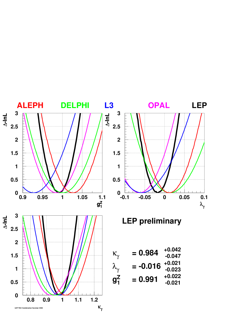
Figure 11.1: The $\log{\cal L}$ curves of the four experiments (thin lines) and the LEP combined curve (thick line) for the three charged TGCs $g_{1}^{\mathrm{Z}}$, $\kappa_{\gamma}$ and $\lambda_{\gamma}$. In each case, the minimal value is subtracted.

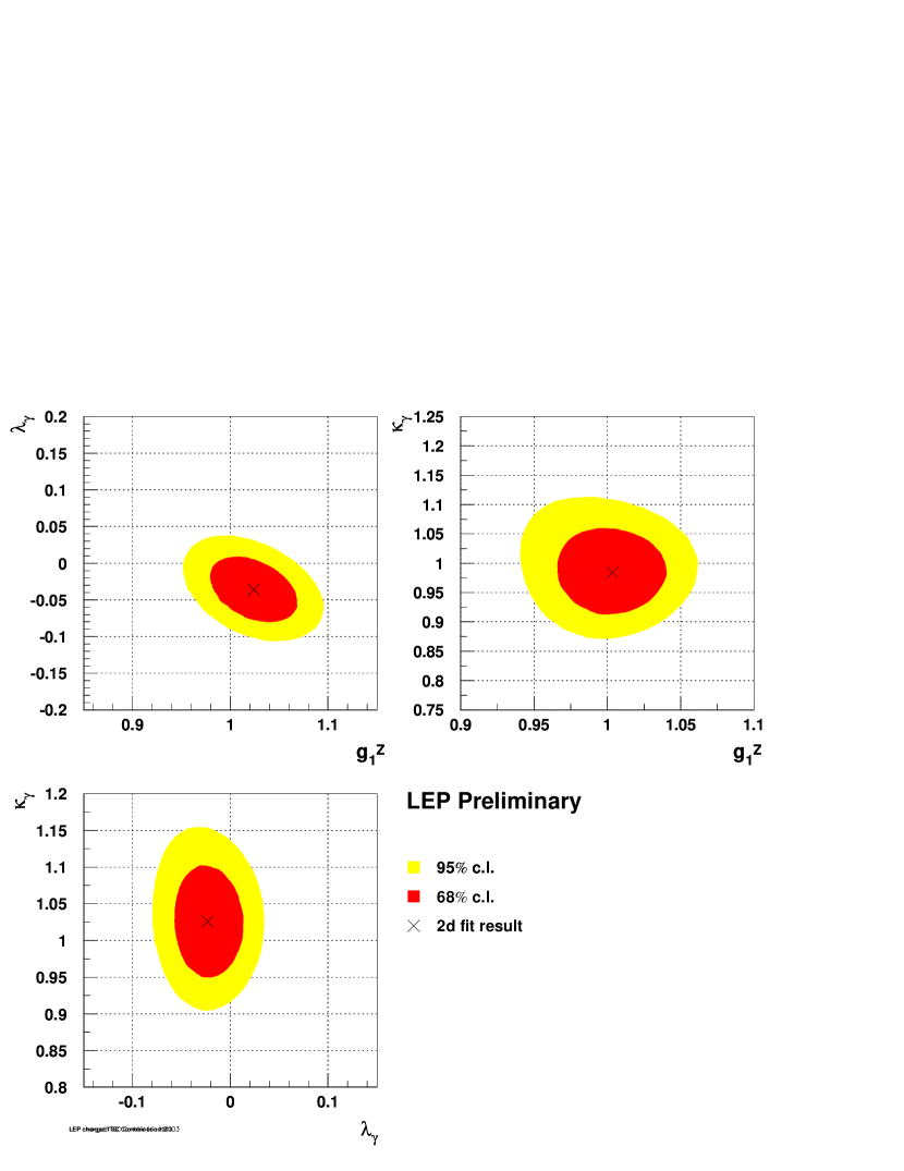
Figure 11.2: The 68% and 95% confidence level contours for the three two-parameter fits to the charged TGCs $g_{1}^{\mathrm{Z}}$-$\lambda_{\gamma}$, $g_{1}^{\mathrm{Z}}$-$\kappa_{\gamma}$ and $\lambda_{\gamma}$-$\kappa_{\gamma}$. The fitted coupling value is indicated with a cross; the Standard Model value for each fit is in the centre of the grid. The contours include the contribution from systematic uncertainties.

11.4.2 Neutral Triple Gauge Boson Couplings in Z$\gamma$ Production

The individual analyses and results of the experiments for the $h$-couplings are described in [188, 189, 190, 191].

Single-Parameter Analyses

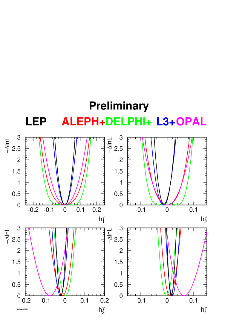
Figure 11.3: The $\log{\cal L}$ curves of the four experiments, and the LEP combined curve for the four neutral TGCs $h_{i}^{\gamma},\leavevmode\nobreak\ i=1,2,3,4$. In each case, the minimal value is subtracted.

The results for each experiment are shown in Table 11.5, where the errors include both statistical and systematic uncertainties. The individual $\log{\cal L}$ curves and their sum are shown in Figures 11.3 and 11.4. The results of the combination are given in Table 11.6. From Figures 11.3 and 11.4 it is clear that the sensitivity of the L3 analysis [190] is the highest amongst the LEP experiments. This is partially due to the use of a larger phase space region, which increases the statistics by about a factor two, and partially due to additional information from using an optimal-observable technique.

Two-Parameter Analyses

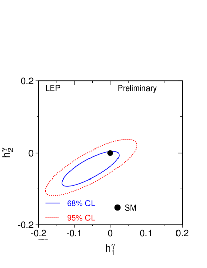
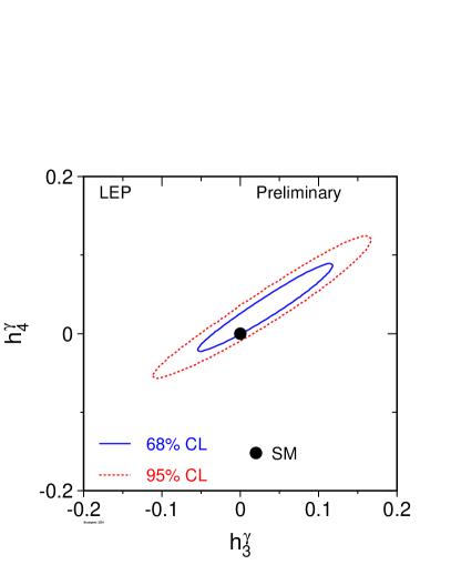
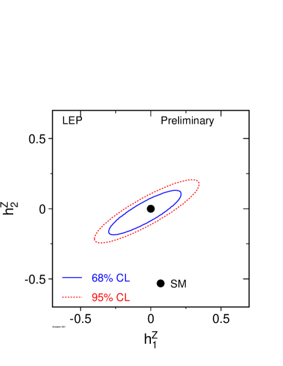
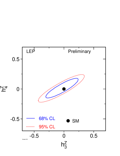
Figure 11.5: Contour curves of 68% C.L. and 95% C.L. in the planes $(h_{1}^{\gamma},h_{2}^{\gamma})$, $(h_{3}^{\gamma},h_{4}^{\gamma})$, $(h_{1}^{Z},h_{2}^{Z})$ and $(h_{3}^{Z},h_{4}^{Z})$ showing the LEP combined result.

The results for each experiment are shown in Table 11.7, where the errors include both statistical and systematic uncertainties. The 68% C.L. and 95% C.L. contour curves resulting from the combinations of the two-dimensional likelihood curves are shown in Figure 11.5. The LEP average values are given in Table 11.8.

Parameter	ALEPH	DELPHI	L3	OPAL
$h_{1}^{\gamma}$	[$-0.14,\leavevmode\nobreak\ \leavevmode\nobreak\ +0.14$]	[$-0.15,\leavevmode\nobreak\ \leavevmode\nobreak\ +0.15$]	[$-0.06,\leavevmode\nobreak\ \leavevmode\nobreak\ +0.06$]	[$-0.13,\leavevmode\nobreak\ \leavevmode\nobreak\ +0.13$]
$h_{2}^{\gamma}$	[$-0.07,\leavevmode\nobreak\ \leavevmode\nobreak\ +0.07$]	[$-0.09,\leavevmode\nobreak\ \leavevmode\nobreak\ +0.09$]	[$-0.053,\leavevmode\nobreak\ \leavevmode\nobreak\ +0.024$]	[$-0.089,\leavevmode\nobreak\ \leavevmode\nobreak\ +0.089$]
$h_{3}^{\gamma}$	[$-0.069,\leavevmode\nobreak\ \leavevmode\nobreak\ +0.037$]	[$-0.047,\leavevmode\nobreak\ \leavevmode\nobreak\ +0.047$]	[$-0.062,\leavevmode\nobreak\ \leavevmode\nobreak\ -0.014$]	[$-0.16,\leavevmode\nobreak\ \leavevmode\nobreak\ +0.00$]
$h_{4}^{\gamma}$	[$-0.020,\leavevmode\nobreak\ \leavevmode\nobreak\ +0.045$]	[$-0.032,\leavevmode\nobreak\ \leavevmode\nobreak\ +0.030$]	[$-0.004,\leavevmode\nobreak\ \leavevmode\nobreak\ +0.045$]	[$+0.01,\leavevmode\nobreak\ \leavevmode\nobreak\ +0.13$]
$h_{1}^{Z}$	[$-0.23,\leavevmode\nobreak\ \leavevmode\nobreak\ +0.23$]	[$-0.24,\leavevmode\nobreak\ \leavevmode\nobreak\ +0.25$]	[$-0.17,\leavevmode\nobreak\ \leavevmode\nobreak\ +0.16$]	[$-0.22,\leavevmode\nobreak\ \leavevmode\nobreak\ +0.22$]
$h_{2}^{Z}$	[$-0.12,\leavevmode\nobreak\ \leavevmode\nobreak\ +0.12$]	[$-0.14,\leavevmode\nobreak\ \leavevmode\nobreak\ +0.14$]	[$-0.10,\leavevmode\nobreak\ \leavevmode\nobreak\ +0.09$]	[$-0.15,\leavevmode\nobreak\ \leavevmode\nobreak\ +0.15$]
$h_{3}^{Z}$	[$-0.28,\leavevmode\nobreak\ \leavevmode\nobreak\ +0.19$]	[$-0.32,\leavevmode\nobreak\ \leavevmode\nobreak\ +0.18$]	[$-0.23,\leavevmode\nobreak\ \leavevmode\nobreak\ +0.11$]	[$-0.29,\leavevmode\nobreak\ \leavevmode\nobreak\ +0.14$]
$h_{4}^{Z}$	[$-0.10,\leavevmode\nobreak\ \leavevmode\nobreak\ +0.15$]	[$-0.12,\leavevmode\nobreak\ \leavevmode\nobreak\ +0.18$]	[$-0.08,\leavevmode\nobreak\ \leavevmode\nobreak\ +0.16$]	[$-0.09,\leavevmode\nobreak\ \leavevmode\nobreak\ +0.19$]

Table 11.5: The 95% C.L. intervals ($\Delta\log{\cal L}=1.92$) measured by the ALEPH, DELPHI, L3 and OPAL. In each case the parameter listed is varied while the remaining ones are fixed to their Standard Model values. Both statistical and systematic uncertainties are included.

Parameter	95% C.L.
$h_{1}^{\gamma}$	[$-0.056,\leavevmode\nobreak\ \leavevmode\nobreak\ +0.055$]
$h_{2}^{\gamma}$	[$-0.045,\leavevmode\nobreak\ \leavevmode\nobreak\ +0.025$]
$h_{3}^{\gamma}$	[$-0.049,\leavevmode\nobreak\ \leavevmode\nobreak\ -0.008$]
$h_{4}^{\gamma}$	[$-0.002,\leavevmode\nobreak\ \leavevmode\nobreak\ +0.034$]
$h_{1}^{Z}$	[$-0.13,\leavevmode\nobreak\ \leavevmode\nobreak\ +0.13$]
$h_{2}^{Z}$	[$-0.078,\leavevmode\nobreak\ \leavevmode\nobreak\ +0.071$]
$h_{3}^{Z}$	[$-0.20,\leavevmode\nobreak\ \leavevmode\nobreak\ +0.07$]
$h_{4}^{Z}$	[$-0.05,\leavevmode\nobreak\ \leavevmode\nobreak\ +0.12$]

Table 11.6: The 95% C.L. intervals ($\Delta\log{\cal L}=1.92$) obtained combining the results from the four experiments. In each case the parameter listed is varied while the remaining ones are fixed to their Standard Model values. Both statistical and systematic uncertainties are included.

Parameter	ALEPH	DELPHI	L3
$h_{1}^{\gamma}$	[$-0.32,\leavevmode\nobreak\ \leavevmode\nobreak\ +0.32$]	[$-0.28,\leavevmode\nobreak\ \leavevmode\nobreak\ +0.28$]	[$-0.17,\leavevmode\nobreak\ \leavevmode\nobreak\ +0.04$]
$h_{2}^{\gamma}$	[$-0.18,\leavevmode\nobreak\ \leavevmode\nobreak\ +0.18$]	[$-0.17,\leavevmode\nobreak\ \leavevmode\nobreak\ +0.18$]	[$-0.12,\leavevmode\nobreak\ \leavevmode\nobreak\ +0.02$]
$h_{3}^{\gamma}$	[$-0.17,\leavevmode\nobreak\ \leavevmode\nobreak\ +0.38$]	[$-0.48,\leavevmode\nobreak\ \leavevmode\nobreak\ +0.20$]	[$-0.09,\leavevmode\nobreak\ \leavevmode\nobreak\ +0.13$]
$h_{4}^{\gamma}$	[$-0.08,\leavevmode\nobreak\ \leavevmode\nobreak\ +0.29$]	[$-0.08,\leavevmode\nobreak\ \leavevmode\nobreak\ +0.15$]	[$-0.04,\leavevmode\nobreak\ \leavevmode\nobreak\ +0.11$]
$h_{1}^{Z}$	[$-0.54,\leavevmode\nobreak\ \leavevmode\nobreak\ +0.54$]	[$-0.45,\leavevmode\nobreak\ \leavevmode\nobreak\ +0.46$]	[$-0.48,\leavevmode\nobreak\ \leavevmode\nobreak\ +0.33$]
$h_{2}^{Z}$	[$-0.29,\leavevmode\nobreak\ \leavevmode\nobreak\ +0.30$]	[$-0.29,\leavevmode\nobreak\ \leavevmode\nobreak\ +0.29$]	[$-0.30,\leavevmode\nobreak\ \leavevmode\nobreak\ +0.22$]
$h_{3}^{Z}$	[$-0.58,\leavevmode\nobreak\ \leavevmode\nobreak\ +0.52$]	[$-0.57,\leavevmode\nobreak\ \leavevmode\nobreak\ +0.38$]	[$-0.43,\leavevmode\nobreak\ \leavevmode\nobreak\ +0.39$]
$h_{4}^{Z}$	[$-0.29,\leavevmode\nobreak\ \leavevmode\nobreak\ +0.31$]	[$-0.31,\leavevmode\nobreak\ \leavevmode\nobreak\ +0.28$]	[$-0.23,\leavevmode\nobreak\ \leavevmode\nobreak\ +0.28$]

Table 11.7: The 95% C.L. intervals ($\Delta\log{\cal L}=1.92$) measured by ALEPH, DELPHI and L3. In each case the two parameters listed are varied while the remaining ones are fixed to their Standard Model values. Both statistical and systematic uncertainties are included.

Parameter	95% C.L.	Correlations
$h_{1}^{\gamma}$	[$-0.16,\leavevmode\nobreak\ \leavevmode\nobreak\ +0.05$]	$1.00$	$+0.79$
$h_{2}^{\gamma}$	[$-0.11,\leavevmode\nobreak\ \leavevmode\nobreak\ +0.02$]	$+0.79$	$1.00$
$h_{3}^{\gamma}$	[$-0.08,\leavevmode\nobreak\ \leavevmode\nobreak\ +0.14$]	$1.00$	$+0.97$
$h_{4}^{\gamma}$	[$-0.04,\leavevmode\nobreak\ \leavevmode\nobreak\ +0.11$]	$+0.97$	$1.00$
$h_{1}^{Z}$	[$-0.35,\leavevmode\nobreak\ \leavevmode\nobreak\ +0.28$]	$1.00$	$+0.77$
$h_{2}^{Z}$	[$-0.21,\leavevmode\nobreak\ \leavevmode\nobreak\ +0.17$]	$+0.77$	$1.00$
$h_{3}^{Z}$	[$-0.37,\leavevmode\nobreak\ \leavevmode\nobreak\ +0.29$]	$1.00$	$+0.76$
$h_{4}^{Z}$	[$-0.19,\leavevmode\nobreak\ \leavevmode\nobreak\ +0.21$]	$+0.76$	$1.00$

Table 11.8: The 95% C.L. intervals ($\Delta\log{\cal L}=1.92$) obtained combining the results from ALEPH, DELPHI and L3. In each case the two parameters listed are varied while the remaining ones are fixed to their Standard Model values. Both statistical and systematic uncertainties are included. Since the shape of the log-likelihood is not parabolic, there is some ambiguity in the definition of the correlation coefficients and the values quoted here are approximate.

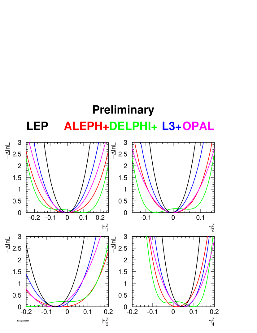
Figure 11.4: The $\log{\cal L}$ curves of the four experiments, and the LEP combined curve for the four neutral TGCs $h_{i}^{Z},\leavevmode\nobreak\ i=1,2,3,4$. In each case, the minimal value is subtracted.

11.4.3 Neutral Triple Gauge Boson Couplings in ZZ Production

The individual analyses and results of the experiments for the $f$-couplings are described in [188, 189, 192, 193].

Single-Parameter Analyses

The results for each experiment are shown in Table 11.9, where the errors include both statistical and systematic uncertainties. The individual $\log{\cal L}$ curves and their sum are shown in Figure 11.6. The results of the combination are given in Table 11.10.

Two-Parameter Analyses

The results from each experiment are shown in Table 11.11, where the errors include both statistical and systematic uncertainties. The 68% C.L. and 95% C.L. contour curves resulting from the combinations of the two-dimensional likelihood curves are shown in Figure 11.7. The LEP average values are given in Table 11.12.

Parameter	ALEPH	DELPHI	L3	OPAL
$f_{4}^{\gamma}$	[$-0.26,\leavevmode\nobreak\ \leavevmode\nobreak\ +0.26$]	[$-0.26,\leavevmode\nobreak\ \leavevmode\nobreak\ +0.28$]	[$-0.28,\leavevmode\nobreak\ \leavevmode\nobreak\ +0.28$]	[$-0.32,\leavevmode\nobreak\ \leavevmode\nobreak\ +0.33$]
$f_{4}^{Z}$	[$-0.44,\leavevmode\nobreak\ \leavevmode\nobreak\ +0.43$]	[$-0.49,\leavevmode\nobreak\ \leavevmode\nobreak\ +0.42$]	[$-0.48,\leavevmode\nobreak\ \leavevmode\nobreak\ +0.46$]	[$-0.45,\leavevmode\nobreak\ \leavevmode\nobreak\ +0.58$]
$f_{5}^{\gamma}$	[$-0.54,\leavevmode\nobreak\ \leavevmode\nobreak\ +0.56$]	[$-0.48,\leavevmode\nobreak\ \leavevmode\nobreak\ +0.61$]	[$-0.39,\leavevmode\nobreak\ \leavevmode\nobreak\ +0.47$]	[$-0.71,\leavevmode\nobreak\ \leavevmode\nobreak\ +0.59$]
$f_{5}^{Z}$	[$-0.73,\leavevmode\nobreak\ \leavevmode\nobreak\ +0.83$]	[$-0.42,\leavevmode\nobreak\ \leavevmode\nobreak\ +0.69$]	[$-0.35,\leavevmode\nobreak\ \leavevmode\nobreak\ +1.03$]	[$-0.94,\leavevmode\nobreak\ \leavevmode\nobreak\ +0.25$]

Table 11.9: The 95% C.L. intervals ($\Delta\log{\cal L}=1.92$) measured by ALEPH, DELPHI, L3 and OPAL. In each case the parameter listed is varied while the remaining ones are fixed to their Standard Model values. Both statistical and systematic uncertainties are included.

Parameter	95% C.L.
$f_{4}^{\gamma}$	[$-0.17,\leavevmode\nobreak\ \leavevmode\nobreak\ +0.19$]
$f_{4}^{Z}$	[$-0.30,\leavevmode\nobreak\ \leavevmode\nobreak\ +0.30$]
$f_{5}^{\gamma}$	[$-0.32,\leavevmode\nobreak\ \leavevmode\nobreak\ +0.36$]
$f_{5}^{Z}$	[$-0.34,\leavevmode\nobreak\ \leavevmode\nobreak\ +0.38$]

Table 11.10: The 95% C.L. intervals ($\Delta\log{\cal L}=1.92$) obtained combining the results from all four experiments. In each case the parameter listed is varied while the remaining ones are fixed to their Standard Model values. Both statistical and systematic uncertainties are included.

Parameter	ALEPH	DELPHI	L3	OPAL
$f_{4}^{\gamma}$	[$-0.26,\leavevmode\nobreak\ \leavevmode\nobreak\ +0.26$]	[$-0.26,\leavevmode\nobreak\ \leavevmode\nobreak\ +0.28$]	[$-0.28,\leavevmode\nobreak\ \leavevmode\nobreak\ +0.28$]	[$-0.32,\leavevmode\nobreak\ \leavevmode\nobreak\ +0.33$]
$f_{4}^{Z}$	[$-0.44,\leavevmode\nobreak\ \leavevmode\nobreak\ +0.43$]	[$-0.49,\leavevmode\nobreak\ \leavevmode\nobreak\ +0.42$]	[$-0.48,\leavevmode\nobreak\ \leavevmode\nobreak\ +0.46$]	[$-0.47,\leavevmode\nobreak\ \leavevmode\nobreak\ +0.58$]
$f_{5}^{\gamma}$	[$-0.52,\leavevmode\nobreak\ \leavevmode\nobreak\ +0.53$]	[$-0.52,\leavevmode\nobreak\ \leavevmode\nobreak\ +0.61$]	[$-0.52,\leavevmode\nobreak\ \leavevmode\nobreak\ +0.62$]	[$-0.67,\leavevmode\nobreak\ \leavevmode\nobreak\ +0.62$]
$f_{5}^{Z}$	[$-0.77,\leavevmode\nobreak\ \leavevmode\nobreak\ +0.86$]	[$-0.44,\leavevmode\nobreak\ \leavevmode\nobreak\ +0.69$]	[$-0.47,\leavevmode\nobreak\ \leavevmode\nobreak\ +1.39$]	[$-0.95,\leavevmode\nobreak\ \leavevmode\nobreak\ +0.33$]

Table 11.11: The 95% C.L. intervals ($\Delta\log{\cal L}=1.92$) measured by ALEPH, DELPHI, L3 and OPAL. In each case the two parameters listed are varied while the remaining ones are fixed to their Standard Model values. Both statistical and systematic uncertainties are included.

Parameter	95% C.L.	Correlations
$f_{4}^{\gamma}$	[$-0.17,\leavevmode\nobreak\ \leavevmode\nobreak\ +0.19$]	$1.00$	$0.07$
$f_{4}^{Z}$	[$-0.30,\leavevmode\nobreak\ \leavevmode\nobreak\ +0.29$]	$0.07$	$1.00$
$f_{5}^{\gamma}$	[$-0.34,\leavevmode\nobreak\ \leavevmode\nobreak\ +0.38$]	$1.00$	$-0.17$
$f_{5}^{Z}$	[$-0.38,\leavevmode\nobreak\ \leavevmode\nobreak\ +0.36$]	$-0.17$	$1.00$

Table 11.12: The 95% C.L. intervals ($\Delta\log{\cal L}=1.92$) obtained combining the results from all four experiments. In each case the two parameters listed are varied while the remaining ones are fixed to their Standard Model values. Both statistical and systematic uncertainties are included. Since the shape of the log-likelihood is not parabolic, there is some ambiguity in the definition of the correlation coefficients and the values quoted here are approximate.

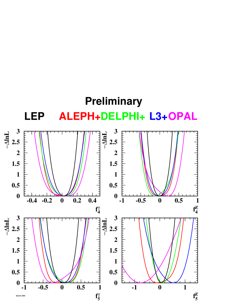
Figure 11.6: The $\log{\cal L}$ curves of the four experiments, and the LEP combined curve for the four neutral TGCs $f_{i}^{V},\leavevmode\nobreak\ V=\gamma,Z,\leavevmode\nobreak\ i=4,5$. In each case, the minimal value is subtracted.

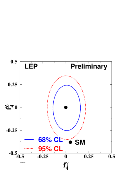
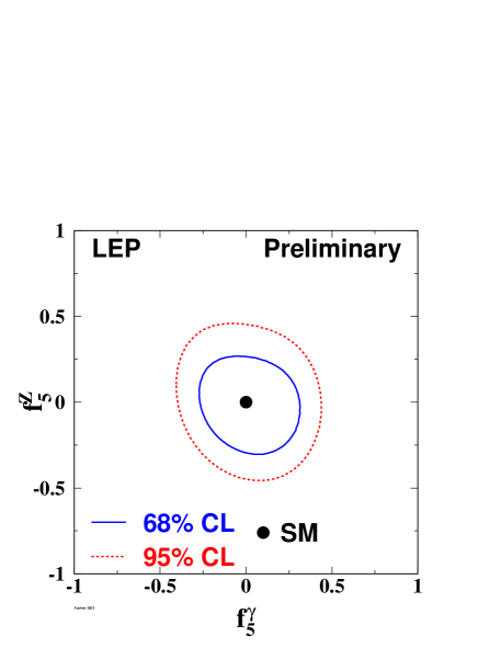
Figure 11.7: Contour curves of 68% C.L. and 95% C.L. in the plane $(f_{4}^{\gamma},f_{4}^{Z})$ and $(f_{5}^{\gamma},f_{5}^{Z})$ showing the LEP combined result.

11.4.4 Quartic Gauge Boson Couplings

The individual numerical results from the experiments participating in the combination, and the combined result are shown in Table 11.13. The corresponding $\log{\cal L}$ curves are shown in Figure 11.8. The errors include both statistical and systematic uncertainties.

Parameter	ALEPH	L3	OPAL	Combined
$a_{c}/\Lambda^{2}$	[$-0.041,\leavevmode\nobreak\ \leavevmode\nobreak\ +0.044$]	[$-0.037,\leavevmode\nobreak\ \leavevmode\nobreak\ +0.054$]	[$-0.045,\leavevmode\nobreak\ \leavevmode\nobreak\ +0.050$]	[$-0.029,\leavevmode\nobreak\ \leavevmode\nobreak\ +0.039$]
$a_{0}/\Lambda^{2}$	[$-0.012,\leavevmode\nobreak\ \leavevmode\nobreak\ +0.019$]	[$-0.014,\leavevmode\nobreak\ \leavevmode\nobreak\ +0.027$]	[$-0.012,\leavevmode\nobreak\ \leavevmode\nobreak\ +0.031$]	[$-0.008,\leavevmode\nobreak\ \leavevmode\nobreak\ +0.021$]

Table 11.13: The limits for the QGCs $a_{c}/\Lambda^{2}$ and $a_{0}/\Lambda^{2}$ associated with the $\mathrm{ZZ}\gamma\gamma$  vertex at 95% confidence level for ALEPH, L3 and OPAL, and the LEP result obtained by combining them. Both statistical and systematic errors are included.

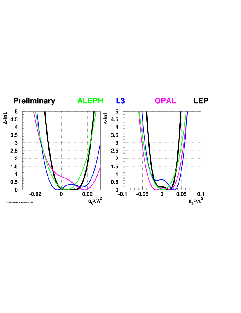
Figure 11.8: The $\log{\cal L}$ curves of L3 and OPAL (thin lines) and the combined curve (thick line) for the QGCs $a_{c}/\Lambda^{2}$ and $a_{0}/\Lambda^{2}$, associated with the $\mathrm{ZZ}\gamma\gamma$   vertex. In each case, the minimal value is subtracted.

Conclusions

Combinations of charged and neutral triple gauge boson couplings, as well as quartic gauge boson couplings associated with the $\mathrm{ZZ}\gamma\gamma$  vertex were made, based on results from the four LEP experiments ALEPH, DELPHI, L3 and OPAL. No significant deviation from the Standard Model prediction is seen for any of the electroweak gauge boson couplings studied. With the LEP-combined charged TGC results, the existence of triple gauge boson couplings among the electroweak gauge bosons is experimentally verified. As an example, these data allow the Kaluza-Klein theory [200], in which $\mbox{$\kappa_{\gamma}$}=-2$, to be excluded completely [201].

Chapter 12 Colour Reconnection in W-Pair Events

Updates with respect to summer 2003:
Unchanged w.r.t. summer 2002: Results are preliminary.

12.1 Introduction

In $\mathrm{W^{+}W^{-}}\rightarrow\mathrm{q\overline{q}}\mathrm{q\overline{q}}$ events, the products of the two (colour singlet) W decays in general have a significant space-time overlap as the separation of their decay vertices, $\tau_{W}\sim 1/\Gamma_{W}\approx 0.1$ fm, is small compared to characteristic hadronic distance scales of $\sim 1$ fm. Colour reconnection, also known as colour rearrangement (CR), was first introduced in[202] and refers to a reorganisation of the colour flow between the two W bosons. A precedent is set for such effects by colour suppressed B meson decays, e.g. $B\rightarrow J/\psi K$, where there is “cross-talk” between the two original colour singlets, $\bar{\mathrm{c}}$+s and c+spectator[202, 203].

QCD interference effects between the colour singlets in $\mathrm{W^{+}W^{-}}$ decays during the perturbative phase are expected to be small, affecting the W mass by $\sim(\frac{\alpha_{\mathrm{S}}}{\pi N_{\mathrm{colours}}})^{2}\Gamma_{W}$ $\sim\cal{O}(\mathrm{1\leavevmode\nobreak\ {\mathrm{Me\kern-1.00006ptV}}})$ [203]. In contrast, non-perturbative effects involving soft gluons with energies less than $\Gamma_{\mathrm{W}}$ may be significant, with effects on $m_{\mathrm{W}}$ $\sim\cal{O}(\mathrm{10\leavevmode\nobreak\ {\mathrm{Me\kern-1.00006ptV}}})$. To estimate the impact of this phenomenon a variety of phenomenological models have been developed [203, 204, 205, 206, 207, 208], some of which are compared with data in this note.

Many observables have been considered in the search for an experimental signature of colour reconnection. The inclusive properties of events such as the mean charged particle multiplicity, distributions of thrust, rapidity, transverse momentum and $\ln(1/x_{p})$ are found to have limited sensitivity[209, 210, 211, 212]. The effects of CR are predicted to be numerically larger in these observables when only higher mass hadrons such as kaons and protons are considered[213]. However, experimental investigations[210, 214] find no significant gain in sensitivity due to the low production rate of such species in W decays and the finite size of the data sample.

More recently, in analogy with the “string effect” analysis in 3-jet $\mathrm{e}^{+}\mathrm{e}^{-}\rightarrow\mathrm{q\overline{q}}g$ events[215], the so-called “particle flow” method [222, 223, 224] has been investigated by all LEP collaborations [225, 226, 227, 228]. In this, pairs of jets in $\mathrm{W^{+}W^{-}}\rightarrow\mathrm{q\overline{q}}\mathrm{q\overline{q}}$ events are associated with the decay of a W, after which four jet-jet regions are chosen: two corresponding to jets sharing the same W parent (intra-W), and two in which the parents differ (inter-W). As there is a two-fold ambiguity in the assignment of inter-W regions, the configuration having the smaller sum of inter-W angles is chosen.

Particles are projected onto the planes defined by these jet pairs and the particle density constructed as a function of $\phi$, the projected angle relative to one jet in each plane. To account for the variation in the opening angles, $\phi_{0}$, of the jet-jet pairs defining each plane, the particle densities in $\phi$ are constructed as functions of normalised angles, $\phi_{r}=\phi/\phi_{0}$, by a simple rescaling of the projected angles for each particle, event by event. Particles having projected angles $\phi$ smaller than $\phi_{0}$ in at least one of the four planes are considered further. This gives particle densities, $\frac{1}{N_{\mathrm{event}}}\frac{\mathrm{d}n}{\mathrm{d}\phi_{r}}$, in four regions with $\phi_{r}$ in the range 0–1, and where $n$ and $N_{\mathrm{event}}$ are the number of particles and events, respectively.

As particle density reflects the colour flow in an event, CR models predict a change in the relative particle densities between inter-W and intra-W regions. On average, colour reconnection is expected to affect the particle densities of both inter-W regions in the same way and so they are added together, as are the two intra-W regions. The observable used to quantify such changes, $R_{N}$, is defined:

$$R_{N}=\frac{\frac{1}{N_{\mathrm{event}}}\int^{0.8}_{0.2}\frac{\mathrm{d}n}{\mathrm{d}\phi_{r}}(\mathrm{intra-W})\mathrm{d}\phi_{r}}{\frac{1}{N_{\mathrm{event}}}\int^{0.8}_{0.2}\frac{\mathrm{d}n}{\mathrm{d}\phi_{r}}(\mathrm{inter-W})\mathrm{d}\phi_{r}}\,.$$ (12.1)

As the effects of CR are expected to be enhanced for low momentum particles far from the jet axis, the range of integration excludes jet cores ($\phi_{r}\approx 0$ and $\phi_{r}\approx 1$). The precise upper and lower limits are optimised by model studies of predicted sensitivity.

Each LEP experiment has developed its own variation on this analysis, differing primarily in the selection of $\mathrm{W^{+}W^{-}}\rightarrow\mathrm{q\overline{q}}\mathrm{q\overline{q}}$ events. In L3[227] and DELPHI[226], events are selected in a very particular configuration (“topological selection”) by imposing restrictions on the jet-jet angles and on the jet resolution parameter for the three- to four-jet transition (Durham or LUCLUS schemes). This selects events which are more planar than those in the inclusive $\mathrm{W^{+}W^{-}}\rightarrow\mathrm{q\overline{q}}\mathrm{q\overline{q}}$ sample and the association between jet pairs and W’s is given by the relative angular separation of the jets. The overall efficiency for selecting events is $\sim 15$%. The ALEPH[225] and OPAL[228] event selections are based on their W mass analyses. Assignment of pairs of jets to W’s also follows that used in measuring $m_{\mathrm{W}}$, using either a 4-jet matrix element [229] or a multivariate algorithm [230]. These latter selections have much higher efficiencies, varying from 45% to 90%, but lead to samples of events having a less planar topology and hence a more complicated colour flow. ALEPH also uses the topological selection for consistency checks.

The data are corrected bin-by-bin for background contamination in the inter-W and intra-W regions separately. The possibility of CR effects existing in background processes, such as $\mathrm{ZZ}\rightarrow\mathrm{q\overline{q}}\mathrm{q\overline{q}}$, is neglected. Since the data are not corrected for the effects of event selection, momentum resolution and finite acceptance, the values of $R_{N}$ measured by the experiments cannot be compared directly with one another. However, it is possible to perform a relative comparison by using a common sample of Monte Carlo events, processed using the detector simulation program of each experiment.

12.2 Combination Procedure

The measured values of $R_{N}$ can be compared after they have been normalised using a common sample of events, processed using the detector simulation and particle flow analysis of each experiment. A variable, $r$, is constructed:

$$r=\frac{R_{N}^{\mathrm{data}}}{R_{N}^{\mathrm{no-CR}}}\,,$$ (12.2)

where $R_{N}^{\mathrm{data}}$ and $R_{N}^{\mathrm{no-CR}}$ are the values of $R_{N}$ measured by each experiment in data and in a common sample of events without CR. In the absence of CR, all experiments should find $r$ consistent with unity. The default no-CR sample used for this normalisation consists of $\mathrm{e}^{+}\mathrm{e}^{-}\rightarrow\mathrm{W^{+}W^{-}}$ events produced using the KORALW[231] event generator and hadronised using either the JETSET[63], ARIADNE[232] or HERWIG[205] model depending on the colour reconnection model being tested. Input from experiments used to perform the combination is given in terms of $R_{N}$ and detailed in Appendix D.1.

12.2.1 Weights

The statistical precision of $R_{N}$ measured by the experiments does not reflect directly the sensitivity to CR, for example the measurements of ALEPH and OPAL have efficiencies several times larger than the topological selections of L3 and DELPHI, yet only yield comparable sensitivity. The relative sensitivity of the experiments may also be model dependent. Therefore, results are averaged using model dependent weights, i.e.

$$w_{i}=\frac{(R^{i}_{N}-R_{N}^{i,\mathrm{no-CR}})^{2}}{\sigma^{2}_{R_{N}}(\mathrm{stat.})+\sigma^{2}_{R_{N}}(\mathrm{syst.})}\,,$$ (12.3)

where $R^{i}_{N}$ and $R_{N}^{i,\mathrm{no-CR}}$ represent the $R_{N}$ values for CR model $i$ and its corresponding no-CR scenario, and $\sigma^{2}_{R_{N}}$ are the total statistical and systematic uncertainties. To test models, $R_{N}$ values using common samples are provided by experiments for each of the following models:

1. SK-I, 100% reconnected (KORALW $+$ JETSET),

2. ARIADNE-II, inter-W reconnection rate about 22% (KORALW $+$ ARIADNE),

3. HERWIG CR, reconnected fraction $\frac{1}{9}$ (KORALW $+$ HERWIG).

Samples in parentheses are the corresponding no-CR scenarios used to define $w_{i}$. In each case, KORALW is used to generate the events at least up to the four-fermion level. These special Monte Carlo samples (called “Cetraro” samples) have been generated with the ALEPH tuned parameters, obtained with hadronic Z decays, and have been processed through the detector simulation of each experiment.

12.2.2 Combination of centre-of-mass energies

The common files required to perform the combination are only available at a single centre-of-mass energy ($E_{\mathrm{cm}}$) of 188.6 GeV. The data from the experiments can only therefore be combined at this energy. The procedure adopted to combine all LEP data is summarised below.

$R_{N}$ is measured in each experiment at each centre-of-mass energy, in both data and Monte Carlo. The predicted variation of $R_{N}$ with centre-of-mass energy is determined separately by each experiment using its own samples of simulated $\mathrm{e}^{+}\mathrm{e}^{-}\rightarrow\mathrm{W^{+}W^{-}}$ events, with hadronisation performed using the no-CR JETSET model. This variation is parametrised by fitting a polynomial to these simulated $R_{N}$. The $R_{N}$ measured in data are subsequently extrapolated to the reference energy of 189 GeV using this function, and the weighted average of the rescaled values in each experiment is used as input to the combination.

12.3 Systematics

The sources of potential systematic uncertainty identified are separated into those which are correlated between experiments and those which are not. For correlated sources, the component correlated between all experiments is assigned as the smallest uncertainty found in any single experiment, with the quadrature remainder treated as an uncorrelated contribution. Preliminary estimates of the dominant systematics on $R_{N}$ are given in Appendix D.1 for each experiment, and described below.

12.3.1 Hadronisation

This is assigned by comparison of the single sample of $\mathrm{W^{+}W^{-}}$ events generated using KORALW, and hadronised with three different models, i.e. JETSET, HERWIG and ARIADNE. The systematic is assigned as the spread of the $R_{N}$ values obtained when using the various models given in Appendix D.1. This is treated as a correlated uncertainty.

12.3.2 Bose-Einstein Correlations

Although a recent analysis by DELPHI reports the observation of inter-W Bose-Einstein correlation (BEC) in $\mathrm{W^{+}W^{-}}\rightarrow\mathrm{q\overline{q}}\mathrm{q\overline{q}}$ events with a significance of 2.9 standard deviations for like-sign pairs and 1.9 standard deviations for unlike-sign pairs [233], analyses by other collaborations[234, 235, 236] find no significant evidence for such effects, see also chapter 13. Therefore, BEC effects are only considered within each W separately. The estimated uncertainty is assigned, using common MC samples, as the difference in $R_{N}$ between an intra-W BEC sample and the corresponding no-BEC sample. This is treated as correlated between experiments.

12.3.3 Background

Background is dominated by the $\mathrm{e}^{+}\mathrm{e}^{-}\rightarrow\mathrm{q\overline{q}}$ process, with a smaller contribution from $\mathrm{ZZ}\rightarrow\mathrm{q\overline{q}}\mathrm{q\overline{q}}$ diagrams. As no common background samples exist, apart from dedicated ones for BEC analyses, experiment specific samples are used. The uncertainty is defined as the difference in the $R_{N}$ value relative to that obtained using the default background model and assumed cross-sections in each experiment.

$\mathrm{e}^{+}\mathrm{e}^{-}\rightarrow\mathrm{q\overline{q}}$

The systematic is separated into two components, one accounting for the shape of the background, the other for the uncertainty in the value of the background cross-section, $\sigma(\mathrm{e}^{+}\mathrm{e}^{-}\rightarrow\mathrm{q\overline{q}})$.

Uncertainty in the shape is estimated by comparing hadronisation models. Experiments typically have large samples simulated using 2-fermion event generators hadronised with various models. This uncertainty is assigned as $\pm\frac{1}{2}$ of the largest difference between any pair of hadronisation models and treated as uncorrelated between experiments.

The second uncertainty arises due to the accuracy of the experimentally measured cross-sections. The systematic is assigned as the larger of the deviations in $R_{N}$ caused when $\sigma(\mathrm{e}^{+}\mathrm{e}^{-}\rightarrow\mathrm{q\overline{q}})$ is varied by $\pm 10$% from its default value. This variation was based on the conclusions of a study comparing four-jet data with models[237], and is significantly larger than the $\sim 1$% uncertainty in the inclusive $\mathrm{e}^{+}\mathrm{e}^{-}\rightarrow\mathrm{q\overline{q}}$ ($\sqrt{s^{\prime}/s}>0.85$) cross-section measured by the LEP2 2-fermion group. It is treated as correlated between experiments.

$\mathrm{ZZ}\rightarrow\mathrm{q\overline{q}}\mathrm{q\overline{q}}$

Similarly to the $\mathrm{e}^{+}\mathrm{e}^{-}\rightarrow\mathrm{q\overline{q}}$ case, this background cross-section is varied by $\pm 15$%. For comparison, the uncertainty on $\sigma(\mathrm{ZZ})$ measured by the LEP2 4-fermion group is $\sim 11$% at $\sqrt{s}\simeq 189$ GeV. It is treated as correlated between experiments.

$\mathrm{W^{+}W^{-}}\rightarrow\mathrm{q\overline{q}}\ell\nu_{\ell}$

Semi-leptonic WW decays which are incorrectly identified as $\mathrm{W^{+}W^{-}}\rightarrow\mathrm{q\overline{q}}\mathrm{q\overline{q}}$ events are the third main category of background, and its contribution is very small. The fraction of $\mathrm{W^{+}W^{-}}\rightarrow\mathrm{q\overline{q}}\ell\nu_{\ell}$ events present in the sample used for the particle flow analysis varies in the range 0.04–2.2% between the experiments. The uncertainty in this background consists of hadronisation effects and also uncertainty in the cross-section. As this source is a very small background relative to those discussed above, and the effect of either varying the cross-section by its measured uncertainty or of changing the hadronisation model do not change the measured $R_{N}$ significantly, this source is neglected.

12.3.4 Detector Effects

The data are not corrected for the effects of finite resolution or acceptance. Various studies have been carried out, e.g. by analysing $\mathrm{W^{+}W^{-}}\rightarrow\mathrm{q\overline{q}}\ell\nu_{\ell}$ events in the same way as $\mathrm{W^{+}W^{-}}\rightarrow\mathrm{q\overline{q}}\mathrm{q\overline{q}}$ events in order to validate the method and the choice of energy flow objects used to measure the particle yields between jets [227]. To take into account the effects of detector resolution and acceptance, ALEPH, L3 and OPAL have studied the impact of changing the object definition entering the particle flow distributions and have assigned a systematic error from the difference in the measured $R_{N}$.

12.3.5 Centre-of-mass energy dependence

As there may be model dependence in the parametrised energy dependence, the second order polynomial used to perform the extrapolation to the reference energy of 189 GeV is usually determined using several different models, with and without colour reconnection. DELPHI, L3 and OPAL use differences relative to the default no-CR model to assign a systematic uncertainty while ALEPH takes the spread of the results obtained with all the models with and without CR which have been used. This error is assumed to be uncorrelated between experiments.

12.3.6 Weighting function

The weighting function of Equation 12.3 could justifiably be modified such that only the uncorrelated components of the systematic uncertainty appear in the denominator. To accommodate this, the average is performed using both variants of the weighting function. This has an insignificant effect on the consistency between data and model under test, e.g. for SK-I the result is changed by 0.02 standard deviations, and this effect is therefore neglected.

12.4 Combined Results

Experiments provide their results in the form of $R_{N}$ (or changes to $R_{N}$) at a reference centre-of-mass energy of 189 GeV by scaling results obtained at various energies using the predicted energy dependence of their own no-CR MC samples. This avoids having to generate common samples at multiple centre-of-mass energies.

The detailed results from all experiments are included in Appendix D.1. These consist of preliminary results, taken from the publicly available notes[225, 226, 227, 228], and additional information from analysis of Monte Carlo samples. The averaging procedure itself is carried out by each of the experiments and good agreement is obtained.

An example of this averaging to test an extreme scenario of the SK-I CR model (full reconnection) is given in Appendix D.3. The average obtained in this case is:

$$r(data) = 0.969\pm 0.011(\mathrm{stat.})\pm 0.009(\mathrm{syst.\leavevmode\nobreak\ corr.})\pm 0.006(\mathrm{syst.\leavevmode\nobreak\ uncorr.})\,,$$ (12.4)

$$r(\mathrm{\mbox{SK-I}}\ 100\%) = 0.8909\,.$$ (12.5)

The measurements of each experiment and this combined result are shown in Figure 12.1. As the sensitivity of the analysis is different for each experiment, the value of $r$ predicted by the SK-I model is indicated separately for each experiment by a dashed line in the figure. Thus the data disagree with the extreme scenario of this particular model at a level of 5.2 standard deviations. The data from the four experiments are consistent with each other and tend to prefer an intermediate colour reconnection scenario rather than the no colour reconnection one at the level of 2.2 standard deviations in the SK-I framework.

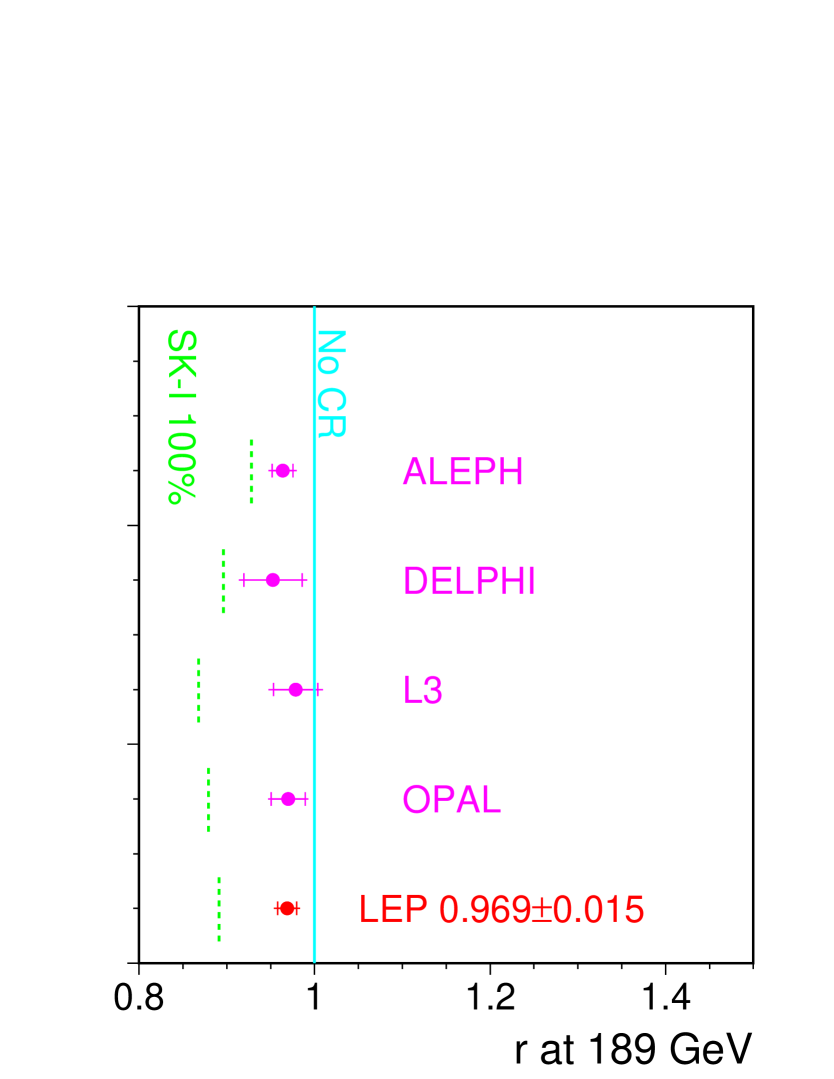
Figure 12.1: Preliminary particle flow results using all data, combined to test the limiting case of the SK-I model in which more than 99.9% of the events are colour reconnected. The error bars correspond to the total error with the inner part showing the statistical uncertainty. The predicted values of $r$ for this CR model are indicated separately for the analysis of each experiment by dashed lines.

12.4.1 Parameter space in SK-I model

In the SK-I model, the reconnection probability is governed by an arbitrary, free parameter, $k_{I}$. By comparing the data with model predictions evaluated at a variety of $k_{I}$ values, it is possible to determine the reconnection probability that is most consistent with data, which can in turn be used to estimate the corresponding bias in the measured $m_{\mathrm{W}}$. By repeating the averaging procedure using model inputs for the set of $k_{I}$ values given in Table D.2, including a re-evaluation of the weights for each value of $k_{I}$, it is found that the data prefer a value of $k_{I}=1.18$ as shown in Figure 12.2. The 68% confidence level lower and upper limits are 0.39 and 2.13 respectively. The LEP averages in $r$ obtained for the different $k_{I}$ values are summarised in Table D.4. They correspond to a preferred reconnection probability of 49% in this model at 189 GeV as illustrated in Figure 12.3.

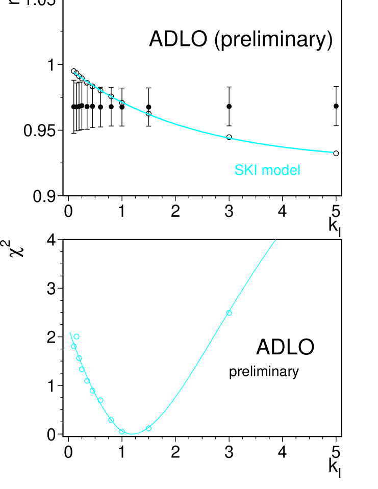
Figure 12.2: Comparison of the LEP average $r$ values with the SK-I model prediction obtained as a function of the $k_{I}$ parameter. The comparisons are performed after extrapolation of data to the reference centre-of-mass energy of 189 GeV. In the upper plot, the solid line is the result of fitting a function of the form $r(k_{I})=p_{1}(1-exp(-p_{2}k_{I}))+p_{3}$ to the MC predictions. The lower plot shows the corresponding $\chi^{2}$ curve obtained from this comparison. The best agreement between the model and the data is obtained when $k_{I}=1.18$.

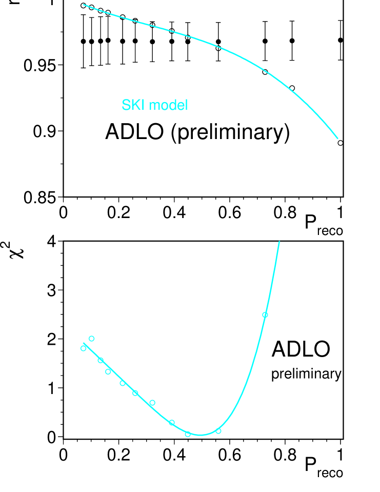
Figure 12.3: Comparison of the LEP average $r$ values with the SK-I model prediction obtained as a function of the reconnection probability. In the upper plot, the solid line is the result of fitting a third order polynomial function to the MC predictions. The lower plot shows a $\chi^{2}$ curve obtained from this comparison using all LEP data at the reference centre-of-mass energy of 189 GeV. The best agreement between the model and the data is obtained when 49% of events are reconnected in this model.

The small variations observed in the LEP average value of $r$ and its corresponding error as a function of $k_{I}$ (or $P_{reco}$) are essentially due to changes in the relative weighting of the experiments.

12.4.2 ARIADNE and HERWIG models

The combination procedure has been applied to common samples of ARIADNE and HERWIG Monte Carlo models. The $R_{N}$ average values obtained with these models based on their respective predicted sensitivity are summarised in Table D.5. The four experiments have observed a weak sensitivity to these colour reconnected samples with the particle flow analysis, as can be seen from Figure 12.4.

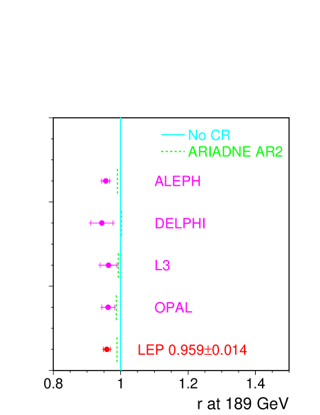
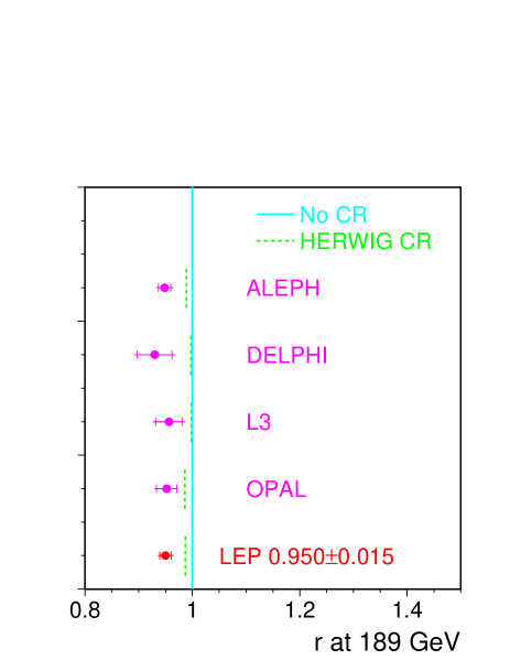
Figure 12.4: Preliminary particle flow results using all data, combined to test the ARIADNE and HERWIG colour reconnection models, based on the predicted sensitivity. The predicted values of $r$ for this CR model are indicated separately for the analysis of each experiment by dashed lines.

12.5 Summary

A first, preliminary combination of the LEP particle flow results is presented, using the entire LEP2 data sample. The data disfavour by 5.2 standard deviations an extreme version of the SK-I model in which colour reconnection has been forced to occur in essentially all events. The combination procedure has been generalised to the SK-I model as a function of its variable reconnection probability. The combined data are described best by the model where 49% of events at 189 GeV are reconnected, corresponding to $k_{I}=1.18$. The LEP data, averaged using weights corresponding to $k_{I}=1.0$, i.e. closest to the optimal fit, do not exclude the no colour reconnection hypothesis, deviating from it by 2.2 standard deviations. A 68% confidence level range has been determined for $k_{I}$ and corresponds to [0.39,2.13].

For both the ARIADNE and HERWIG models, which do not contain adjustable colour reconnection parameters, differences between the results of the colour reconnected and the no-CR scenarios are small and do not allow the particle flow analysis to discriminate between them. To test consistency between data and the no-CR models, the data are averaged using weights where the factor accounting for predicted sensitivity to a given CR model has been set to unity. The $R_{N}$ values obtained with the no colour reconnection HERWIG and ARIADNE models, using the common Cetraro samples, differ from the measured data value by 3.7 and 3.1 standard deviations.

The observed deviations of the $R_{N}$ values from all no colour reconnection models may indicate a possible systematic effect in the description of particle flow for 4-jet events. Independent studies of particle flow in WW semileptonic events as well as other CR-oriented analyses are required to investigate this.

Chapter 13 Bose-Einstein Correlations in W-Pair Events

Updates with respect to summer 2003:
Unchanged w.r.t. summer 2003: Results are preliminary.

13.1 Introduction

The LEP experiments have measured the strength of particle correlations between two hadronic systems obtained from W-pair decay occuring close in space-time at LEP-II. The work presented in this chapter is focused on so-called Bose-Einstein (BE) correlations, i.e., the enhanced probability of production of pairs (multiplets) of identical mesons close together in phase space. The effect is readily observed in particle physics, in particular in hadronic decays of the Z boson, and is qualitatively understood as a result of quantum-mechanical interference originating from the symmetry of the amplitude of the particle production process under exchange of identical mesons.

The presence of correlations between hadrons coming from the decay of a $\mathrm{W^{+}W^{-}}$ pair, in particular those between hadrons originating from different Ws, can affect the direct reconstruction of the mass of the initial W bosons. The measurement of the strength of these correlations can be used for the estimation of the systematic uncertainty of the W mass measurement.

13.2 Method

The principal method [238], called “mixing method”, used in this measurement is based on the direct comparison of 2-particle spectra of genuine hadronic WW events and of mixed WW events. The latter are constructed by mixing the hadronic parts of two semileptonic WW events (first used in  [239]). Such a reference sample has the advantage of reproducing the correlations between particles belonging to the same W, while the particles from different Ws are uncorrelated by construction.

This method gives a model-independent estimate of the interplay between the two hadronic systems, for which BE correlations and also colour reconnection are considered as dominant sources. The possibility of establishing the strength of inter-W correlations in a model-independent way is rather unique; most correlations do carry an inherent model dependence on the reference sample. In the present measurement, the model dependence is limited to the background subtraction.

13.3 Distributions

The two-particle correlations are evaluated using two-particle densities defined in terms of the 4-momentum transfer $Q=\sqrt{-(p_{1}-p_{2})^{2}}$, where $p_{1},p_{2}$ are the 4-momenta of the two particles:

$$\rho_{2}(Q)=\frac{1}{N_{ev}}\frac{dn_{pairs}}{dQ}$$ (13.1)

Here $n_{pairs}$ stands for number of like-sign (unlike-sign) 2-particle permutations. In the case of two stochastically independent hadronically decaying Ws the two-particle inclusive density is given by:

$$\rho_{2}^{WW}\leavevmode\nobreak\ =\leavevmode\nobreak\ \rho_{2}^{W^{+}}+\rho_{2}^{W^{-}}+2\rho_{2}^{mix},$$ (13.2)

where $\rho_{2}^{mix}$ can be expressed via single-particle inclusive density $\rho_{1}(p)$ as:

$$\rho_{2}^{mix}(Q)\leavevmode\nobreak\ =\leavevmode\nobreak\ \int d^{4}p_{1}d^{4}p_{2}\rho^{W^{+}}(p_{1})\rho^{W^{-}}(p_{2})\delta(Q^{2}+(p_{1}-p_{2})^{2})\delta(p_{1}^{2}-m_{\pi}^{2})\delta(p_{2}^{2}-m_{\pi}^{2}).$$ (13.3)

Assuming further that:

$$\rho_{2}^{W^{+}}(Q)\leavevmode\nobreak\ =\leavevmode\nobreak\ \rho_{2}^{W^{-}}(Q)\leavevmode\nobreak\ =\leavevmode\nobreak\ \rho_{2}^{W}(Q),$$ (13.4)

we obtain:

$$\rho_{2}^{WW}(Q)\leavevmode\nobreak\ =\leavevmode\nobreak\ 2\rho_{2}^{W}(Q)+2\rho_{2}^{mix}(Q).$$ (13.5)

In the mixing method, we obtain $\rho_{2}^{mix}$ by combining two hadronic W systems from two different semileptonic WW events. The direct search for inter-W BE correlations is done using the difference of 2-particle densities:

$$\Delta\rho(Q)\leavevmode\nobreak\ =\leavevmode\nobreak\ \rho_{2}^{WW}(Q)-2\rho_{2}^{W}(Q)-2\rho_{2}^{mix}(Q),$$ (13.6)

or, alternatively, their ratio:

$$D(Q)\leavevmode\nobreak\ =\leavevmode\nobreak\ \frac{\rho_{2}^{WW}(Q)}{2\rho_{2}^{W}(Q)+2\rho^{mix}(Q)}\leavevmode\nobreak\ =\leavevmode\nobreak\ 1+\frac{\Delta\rho(Q)}{2\rho_{2}^{W}(Q)+2\rho^{mix}(Q)}.$$ (13.7)

In case of $\Delta\rho(Q)$, we look for a deviation from 0, while in case of $D(Q)$, inter-W BE correlations would manifest themselves by deviation from 1. The event mixing procedure may introduce artificial distortions, or may not fully account for some detector effects or for correlations other than BE correlations, causing a deviation of $\Delta\rho(Q)$ from zero or D from unity for data as well as Monte Carlo without inter-W BE correlations. These possible effects are reduced by using the double ratio or the double difference:

$$D^{\prime}(Q)\leavevmode\nobreak\ =\leavevmode\nobreak\ \frac{D(Q)_{data}}{D(Q)_{MC,nointer}}\hskip 5.69046pt,\hskip 28.45274pt\Delta\rho^{\prime}(Q)\leavevmode\nobreak\ =\leavevmode\nobreak\ \Delta\rho(Q)_{data}-\Delta\rho(Q)_{MC,nointer}\hskip 5.69046pt,$$ (13.8)

where $D(Q)_{MC,nointer}$ and $\Delta\rho(Q)_{MC,nointer}$ are derived from a MC without inter-W BE correlations.

In addition to the mixing method, ALEPH [240] also uses the double ratio of like-sign pairs ($N_{\pi}^{++,--}(Q)$) and unlike-sign pairs $N_{\pi}^{+-}(Q)$ corrected with Monte-Carlo simulations not including BE effects:

$$R^{*}(Q)\leavevmode\nobreak\ =\leavevmode\nobreak\ \left.\left(\frac{N_{\pi}^{++,--}(Q)}{N_{\pi}^{+-}(Q)}\right)^{data}\right/\left(\frac{N_{\pi}^{++,--}(Q)}{N_{\pi}^{+-}(Q)}\right)^{MC}_{noBE}.$$ (13.9)

13.4 Results

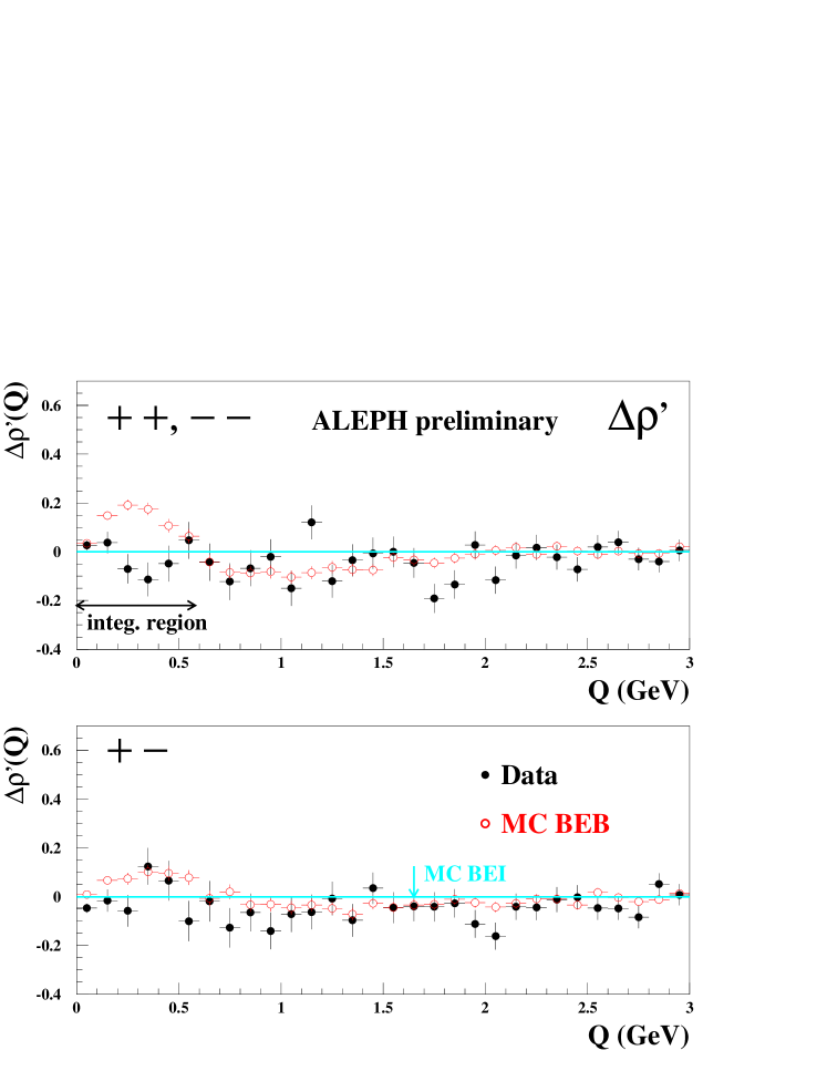
Figure 13.1: Distribution of the quantity $\Delta\rho^{\prime}$ for like- and unlike-sign pairs as a function of $Q$ as measured by the ALEPH collaboration.

Four LEP experiment have submitted results applying the mixing method to the full LEP2 data sample. As examples, the distributions of $\Delta\rho$ measured by ALEPH [241], D measured by DELPHI [233], D and D’ measured by L3 [235] and $\Delta\rho$ measured by OPAL [242] are shown in Figures 13.1, 13.2, 13.3 and 13.4, respectively. In addition ALEPH have submitted results using $R^{*}(Q)$ variable based on data collected at centre-of-mass energies up to $189\leavevmode\nobreak\ {\mathrm{Ge\kern-1.00006ptV}}$ [240].

A simple combination procedure is available through a $\chi^{2}$ average of the numerical results of each experiment with respect to a specific BE model under study, here based on comparisons with various (tuned) versions of the LUBOEI model [243, 244, 241, 233, 235, 242]. The tuning is performed by adjusting the parameters of the model to reproduce correlations in samples of Z⁰ and semileptonic W decays, and applying identical parameters to the modelling of inter-W correlations (so-called “full BE” scenario). In this way the tuning of each experiment takes into account detector systematics in track measurements of different experiments.

An important advantage of the combination procedure used here is that it allows the combination of results obtained using different analyses. The combination procedure assumes a linear dependence of the observed size of BE correlations on various estimators used to analyse the different distributions. It is also verified that there is a linear dependence between the measured W mass shift and the values of these estimators [245]. The estimators are: the integral of the $\Delta\rho(Q)$ distribution (ALEPH, L3, OPAL); the parameter $\Lambda$ when fitting the function $N(1+\delta Q)(1+\Lambda\exp(-k^{2}Q^{2}))$ to the $D^{\prime}(Q)$ distribution, with $N$ fixed to unity (L3), or $\delta$ fixed to zero and $k$ fixed to the value obtained from a fit to the full BE sample (ALEPH); the parameter $\Lambda$ when fitting the function $N(1+\delta Q)(1+\Lambda\exp(-RQ))$ to the $D(Q)$ distribution, with $R$ fixed to the value obtained from a fit to the full BE sample (DELPHI, L3); and finally the integral of the term describing the BE correlation part, $\int\lambda\exp(-\sigma^{2}Q^{2})$, when fitting the function $\kappa(1+\epsilon Q)(1+\lambda\exp(-\sigma^{2}Q^{2}))$ to the $R^{*}(Q)$ distribution (ALEPH).

The size of the correlations for like-sign pairs of particles measured in terms of these estimators is compared with the values expected in the model with and without inter-W correlations in Table 13.1. Table 13.2 summarizes the normalized fractions of the model seen. Note that DELPHI also finds a 1.9 standard deviation effect for pairs of unlike-sign particles from different W bosons[233], similar to the prediction of the LUBOEI model with full strength correlations.

For the combination of the above measurements one has to take into account correlations between them. Correlations between results of the same experiment are strong and are not available. It is however found, for example, that taking reasonable value of these correlations and combining three ALEPH measurements, one obtaines the normalized fractions of the model seen very close to the one of the most precise measurement. Therefore, for simplicity, the combination of the most precise measurements of each experiment is made here: D’ from ALEPH, D from Delphi, D’ from L3 and $\Delta\rho$ from OPAL. In this combination only the uncertainties in the understanding of the background contribution in the data are treated as correlated between experiments (denoted as “corr. syst.” in Table 13.1). The combination via a MINUIT fit gives:

$$\frac{\mathrm{data-model(noBE)}}{\mathrm{model(fullBE)-model(noBE)}}\leavevmode\nobreak\ =\leavevmode\nobreak\ 0.23\pm 0.13\,,$$ (13.10)

where “noBE” includes correlations between decay products of each W, but not the ones between decay products of different Ws and “fullBE” includes all the correlations. A $\chi^{2}$/dof=5.4/3 of the fit is observed. The measurements and their average are shown in Figure 13.5. The measurements used in the combination are marked with arrow.

	data–noBE	stat.	syst.	corr. syst.	fullBE–noBE	Ref.
ALEPH (fit to D’)	$-$0.001	0.015	0.014	0.002	0.077	[241]
ALEPH (integral of $\Delta\rho$)	$-$0.124	0.148	0.200	0.001	0.720	[241]
ALEPH (fit to $R^{*}$)	$-$0.004	0.0062	0.0036	negligible	0.0177	[240]
DELPHI (fit to $D$)	$+$0.241	0.075	0.038	0.017	0.36	[233]
L3 (fit to $D^{\prime}$)	$+$0.008	0.018	0.012	0.004	0.103	[235]
L3 (integral of $\Delta\rho$)	$+$0.03	0.33	0.15	0.055	1.38	[235]
OPAL (integral of $\Delta\rho$)	$-$0.01	0.27	0.21	negligible	0.77	[242]
OPAL (fit to D)	$+$0.069	0.105	0.069	0.010	0.139	[242]

Table 13.1: An overview of the input values for the $\chi^{2}$ combination: the difference between the measured correlations and the model without inter-W correlations (data–noBE), the corresponding statistical (stat.) and total systematic (syst.) errors, the correlated systematic error contribution (corr. syst.), and the difference between “full BE” and “no BE” scenario.

	fraction of the model	stat.	syst.
ALEPH (fit to D’)	$-$0.01	0.19	0.18
ALEPH (integral of $\Delta\rho$)	$-$0.17	0.21	0.28
ALEPH (fit to $R^{*}$)	$-$0.23	0.35	0.20
DELPHI (fit to $D$)	$+$0.67	0.21	0.11
L3 (fit to $D^{\prime}$)	$+$0.08	0.17	0.12
L3 (integral of $\Delta\rho$)	$+$0.02	0.24	0.11
OPAL (integral of $\Delta\rho$)	$-$0.01	0.35	0.27
OPAL (fit to $D$)	$+$0.50	0.76	0.50

Table 13.2: The measured size of correlations expressed as the relative fraction of the model with inter-W correlations.

The result of the $\chi^{2}$ combination of the measurements can be translated into a 68% confidence level upper limit on the shift of the W mass measurements due to the BE correlations between particles from different Ws, $\Delta m_{\mathrm{W}}$, assuming a linear dependence of $\Delta m_{\mathrm{W}}$ on the size of the correlation. For the specific BE model investigated, LUBOEI, a shift of $-35\leavevmode\nobreak\ {\mathrm{Me\kern-1.00006ptV}}$ in the W mass is obtained at full BE correlation strength[246]. Thus the preliminary 68% CL upper limit on the magnitude of the mass shift within the LUBOEI model is:

$$|\Delta m_{\mathrm{W}}| = (0.23+0.13)\cdot 35\leavevmode\nobreak\ {\mathrm{Me\kern-1.00006ptV}}\leavevmode\nobreak\ =\leavevmode\nobreak\ 13\leavevmode\nobreak\ {\mathrm{Me\kern-1.00006ptV}}\leavevmode\nobreak\ \leavevmode\nobreak\ (+1\leavevmode\nobreak\ \sigma\leavevmode\nobreak\ \mathrm{limit})\,.$$ (13.11)

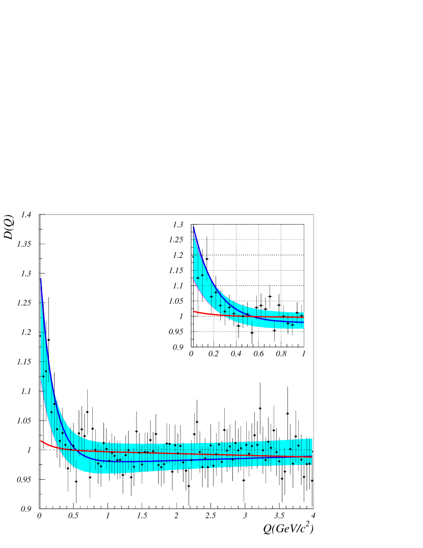
Figure 13.2: Distributions of the quantity D for like-sign pairs as a function of $Q$ as measured by the DELPHI collaboration.The shadowed region shows the fit results.

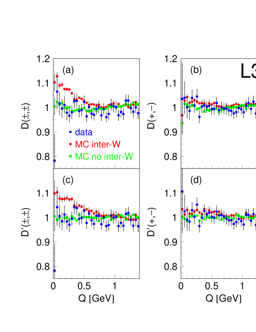
Figure 13.3: Distributions of the quantity D and D’ for like- and unlike-sign pairs as a function of $Q$ as measured by the L3 collaboration.

Figure 13.4: Distribution of the quantity $\Delta\rho$ for like- and unlike-sign pairs as a function of $Q$ as measured by the OPAL collaboration.

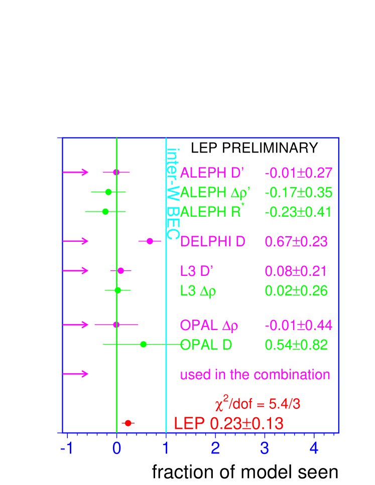
Figure 13.5: $\chi^{2}$ combination of the measured size of correlations expressed as the relative fraction of the model with inter-W correlations.

Chapter 14 W-Boson Mass and Width at LEP-II

Updates with respect to summer 2003:
Unchanged w.r.t. summer 2003: Results are preliminary.

14.1 Introduction

The W boson mass and width results presented in this chapter are obtained from data recorded over a range of centre-of-mass energies, $\sqrt{s}=161-209$ GeV, during the 1996-2000 operation of the LEP collider. The results reported by the ALEPH, DELPHI and L3 collaborations include an analysis of the year 2000 data, and have an integrated luminosity per experiment of about $700$ $\mathrm{pb^{-1}}$. The OPAL collaboration has analysed the data up to and including 1999 and has an integrated luminosity of approximately $450$ $\mathrm{pb^{-1}}$. The ALEPH result does not include an analysis of the small amount of data (about $10$ $\mathrm{pb^{-1}}$) collected in 1996 at a centre-of-mass energy of 172 GeV.

The results on the W mass and width quoted below correspond to a definition based on a Breit-Wigner denominator with an $s$-dependent width, $|(s-m_{\mathrm{W}}^{2})+is\mbox{$\Gamma_{\mathrm{W}}$}/m_{\mathrm{W}}|$.

14.2 W Mass Measurements

Since 1996 the LEP $\mathrm{e}^{+}\mathrm{e}^{-}$ collider has been operating above the threshold for $\mathrm{W^{+}W^{-}}$ pair production. Initially, 10 $\mathrm{pb^{-1}}$ of data were recorded close to the $\mathrm{W^{+}W^{-}}$ pair production threshold. At this energy the $\mathrm{W^{+}W^{-}}$ cross section is sensitive to the W boson mass, $m_{\mathrm{W}}$. Table 14.1 summarises the W mass results from the four LEP collaborations based on these data [247].

THRESHOLD ANALYSIS [247]
Experiment	$m_{\mathrm{W}}$(threshold)/GeV
ALEPH	$80.14\pm 0.35$
DELPHI	$80.40\pm 0.45$
L3	$80.80^{+0.48}_{-0.42}$
OPAL	$80.40^{+0.46}_{-0.43}$

Table 14.1: W mass measurements from the $\mathrm{W^{+}W^{-}}$ threshold cross section at $\sqrt{s}=161$ GeV. The errors include statistical and systematic contributions.

Subsequently LEP has operated at energies significantly above the $\mathrm{W^{+}W^{-}}$ threshold, where the $\mathrm{e}^{+}\mathrm{e}^{-}\rightarrow\mathrm{W^{+}W^{-}}$ cross section has little sensitivity to $m_{\mathrm{W}}$. For these higher energy data $m_{\mathrm{W}}$ is measured through the direct reconstruction of the W boson’s invariant mass from the observed jets and leptons. Table 14.2 summarises the W mass results presented individually by the four LEP experiments using the direct reconstruction method. The combined values of $m_{\mathrm{W}}$ from each collaboration take into account the correlated systematic uncertainties between the decay channels and between the different years of data taking. In addition to the combined numbers, each experiment presents mass measurements from $\mathrm{W^{+}W^{-}}$$\rightarrow$$\mathrm{q\overline{q}}$$\ell\overline{\nu}_{\ell}$ and $\mathrm{W^{+}W^{-}}$$\rightarrow$$\mathrm{q\overline{q}}$$\mathrm{q\overline{q}}$ channels separately. The DELPHI and OPAL collaborations provide results from independent fits to the data in the $\mathrm{q\overline{q}}$$\ell\overline{\nu}_{\ell}$ and $\mathrm{q\overline{q}}$$\mathrm{q\overline{q}}$ decay channels separately and hence account for correlations between years but do not need to include correlations between the two channels. The $\mathrm{q\overline{q}}$$\ell\overline{\nu}_{\ell}$ and $\mathrm{q\overline{q}}$$\mathrm{q\overline{q}}$ results quoted by the ALEPH and L3 collaborations are obtained from a simultaneous fit to all data which, in addition to other correlations, takes into account the correlated systematic uncertainties between the two channels. The L3 result is unchanged when determined through separate fits. The systematic uncertainties in the $\mathrm{W^{+}W^{-}}$$\rightarrow$$\mathrm{q\overline{q}}$$\mathrm{q\overline{q}}$ channel show a large variation between experiments; this is caused by differing estimates of the possible effects of Colour Reconnection (CR) and Bose-Einstein Correlations (BEC), discussed below. The systematic errors in the $\mathrm{W^{+}W^{-}}$$\rightarrow$$\mathrm{q\overline{q}}$$\ell\overline{\nu}_{\ell}$ channel are dominated by uncertainties from hadronisation, with estimates ranging from 15 to 30 ${\mathrm{Me\kern-1.00006ptV}}$.

The results presented in this note differ from those in the previous combination [76] due to revised measurements from the ALEPH Collaboration [248]; otherwise the results are identical. The ALEPH measurements have been revised due to a change in their event reconstruction algorithm. This change makes the analysis less sensitive to detector simulation inaccuracies which were not taken into account in their previous preliminary result.

	DIRECT RECONSTRUCTION
	$\mathrm{W^{+}W^{-}}$$\rightarrow$$\mathrm{q\overline{q}}$$\ell\overline{\nu}_{\ell}$	$\mathrm{W^{+}W^{-}}$$\rightarrow$$\mathrm{q\overline{q}}$$\mathrm{q\overline{q}}$	Combined
Experiment	$m_{\mathrm{W}}$/GeV	$m_{\mathrm{W}}$/GeV	$m_{\mathrm{W}}$/GeV
ALEPH [248]	$80.375\pm 0.062$	$80.431\pm 0.117$	$80.385\pm 0.058$
DELPHI [249, 250, 251, 252]	$80.414\pm 0.089$	$80.374\pm 0.119$	$80.402\pm 0.075$
L3 [253, 254, 255, 256, 257]	$80.314\pm 0.087$	$80.485\pm 0.127$	$80.367\pm 0.078$
OPAL[258, 259, 260, 261, 262]	$80.516\pm 0.073$	$80.407\pm 0.120$	$80.495\pm 0.067$

Table 14.2: Preliminary W mass measurements from direct reconstruction ($\sqrt{s}=172-209$ GeV). Results are given for the semi-leptonic, fully-hadronic channels and the combined value. The $\mathrm{W^{+}W^{-}}$$\rightarrow$$\mathrm{q\overline{q}}$$\ell\overline{\nu}_{\ell}$ results from the OPAL collaboration include mass information from the $\mathrm{W^{+}W^{-}}$$\rightarrow$$\ell\overline{\nu}_{\ell}$$\ell\overline{\nu}_{\ell}$ channel. The results given here differ from those in the publications of the individual experiments as they have been recalculated imposing common FSI uncertainties.

14.3 Combination Procedure

A combined LEP W mass measurement is obtained from the results of the four experiments. In order to perform a reliable combination of the measurements, a more detailed input than that given in Table 14.2 is required. Each experiment provided a W mass measurement for both the $\mathrm{W^{+}W^{-}}$$\rightarrow$$\mathrm{q\overline{q}}$$\ell\overline{\nu}_{\ell}$ and $\mathrm{W^{+}W^{-}}$$\rightarrow$$\mathrm{q\overline{q}}$$\mathrm{q\overline{q}}$ channels for each of the data taking years (1996-2000) that it had analysed. In addition to the four threshold measurements a total of 36 direct reconstruction measurements are supplied: DELPHI provided 10 measurements (1996-2000), L3 gave 8 measurements (1996-2000) having already combined the 1996 and 1997 results, ALEPH provided 8 measurements (1997-2000) and OPAL also gave 8 measurements (1996-1999). The $\mathrm{W^{+}W^{-}}$$\rightarrow$$\ell\overline{\nu}_{\ell}$$\ell\overline{\nu}_{\ell}$ channel is also analysed by the OPAL(1997-1999) collaboration; the lower precision results obtained from this channel are combined with the $\mathrm{W^{+}W^{-}}$$\rightarrow$$\mathrm{q\overline{q}}$$\ell\overline{\nu}_{\ell}$ channel mass determinations.

Subdividing the results by data-taking years enables a proper treatment of the correlated systematic uncertainty from the LEP beam energy and other dependences on the centre-of-mass energy or data-taking period. A detailed breakdown of the sources of systematic uncertainty are provided for each result and the correlations specified. The inter-year, inter-channel and inter-experiment correlations are included in the combination. The main sources of correlated systematic errors are: colour reconnection, Bose-Einstein correlations, hadronisation, the LEP beam energy, and uncertainties from initial and final state radiation. The full correlation matrix for the LEP beam energy is employed[263]. The combination is performed and the evaluation of the components of the total error assessed using the Best Linear Unbiased Estimate (BLUE) technique, see Reference 81.

Figure 14.1: W mass bias obtained in the SK-I model of colour reconnection relative to a simulation without colour reconnection as a function of the fraction of events reconnected for the fully-hadronic decay channel at a centre of mass energy of 189 GeV. The analyses of the four LEP experiments show similar sensitivity to this effect. The points connected by the lines have correlated uncertainties increasing to the right in the range indicated.

A preliminary study of colour reconnection has been made by the LEP experiments using the particle flow method [264] on a sample of fully-hadronic WW events, see chapter 12. These results are interpreted in terms of the reconnection parameter $k_{i}$ of the SK-I model [265] and yield a $68\%$ confidence level range of:

$$0.39<k_{i}<2.13\,.$$ (14.1)

The method was found to be insensitive to the HERWIG and ARIADNE-II models of colour reconnection.

Figure 14.2: The values used in the W Mass combination for the uncertainty due to colour reconnection are shown as a function of the centre of mass energy. These values were obtained from a linear fit to simulation results obtained with the SK1 model of colour reconnection at $k_{i}=2.13$.

Studies of simulation samples have demonstrated that the four experiments are equally sensitive to colour reconnection effects, i.e. when looking at the same CR model similar biases are seen by all experiments. This is shown in Figure 14.1 for the SKI model as a function of the fraction of reconnected events. For this reason a common value for all experiments of the CR systematic uncertainty is used in the combination.

For this combination, no offset has been applied to the central value of $m_{\mathrm{W}}$ due to colour reconnection effects and a symmetric systematic error has been imposed. The $m_{\mathrm{W}}$ error is set from a linear extrapolation of simulation results obtained at $k_{i}=2.13$, the values used in the combination ere: $74\leavevmode\nobreak\ {\mathrm{Me\kern-1.00006ptV}}$ shift for the 1996 data at a centre-of-mass energy of $172\leavevmode\nobreak\ {\mathrm{Ge\kern-1.00006ptV}}$, $84\leavevmode\nobreak\ {\mathrm{Me\kern-1.00006ptV}}$ for 1997 at $183\leavevmode\nobreak\ {\mathrm{Ge\kern-1.00006ptV}}$, $90\leavevmode\nobreak\ {\mathrm{Me\kern-1.00006ptV}}$ for 1998 at $189\leavevmode\nobreak\ {\mathrm{Ge\kern-1.00006ptV}}$, $95\leavevmode\nobreak\ {\mathrm{Me\kern-1.00006ptV}}$ for 1999 at $195\leavevmode\nobreak\ {\mathrm{Ge\kern-1.00006ptV}}$ and $105\leavevmode\nobreak\ {\mathrm{Me\kern-1.00006ptV}}$ for 2000 at $207\leavevmode\nobreak\ {\mathrm{Ge\kern-1.00006ptV}}$, they are shown in Figure 14.2. Previous $m_{\mathrm{W}}$ combinations have relied upon theoretical expectations of colour reconnection effects, in which there is considerable uncertainty. This new data driven approach achieves a more robust uncertainty estimate at the expense of a significantly increased colour reconnection uncertainty. The ARIADNE-II and HERWIG models of colour reconnection have also been studied and the W Mass shift was found to be lower than that from SK1 with $k_{i}=2.13$ used for the combination.

For Bose-Einstein correlations, a similar test has been made of the respective experimental sensitivities with the LUBOEI [266] model: the experiments observed compatible mass shifts. A common value of the systematic uncertainty from BEC of 35 MeV is assumed from studies of the LUBOEI model. This value may be compared with recent direct measurements from LEP of this effect, Chapter 13, where the observed Bose-Einstein effect was of smaller magnitude than in the LUBOEI model, see chapter 13. Hence, the currently assigned 35 MeV uncertainty is considered a conservative estimate.

14.4 LEP Combined W Boson Mass

The combined W mass from direct reconstruction is

$$m_{\mathrm{W}}(\mathrm{direct})=80.412\pm 0.029(\mathrm{stat.})\pm 0.031(\mathrm{syst.})\leavevmode\nobreak\ {\mathrm{Ge\kern-1.00006ptV}},$$ (14.2)

with a $\chi^{2}$/d.o.f. of 28.2/33, corresponding to a $\chi^{2}$ probability of 70%. The weight of the fully-hadronic channel in the combined fit is 0.10. This reduced weight is a consequence of the relatively large size of the current estimates of the systematic errors from CR and BEC. Table 14.3 gives a breakdown of the contribution to the total error of the various sources of systematic errors. The largest contribution to the systematic error comes from hadronisation uncertainties, which are conservatively treated as correlated between the two channels, between experiments and between years. In the absence of systematic effects the current LEP statistical precision on $m_{\mathrm{W}}$ would be $21$ ${\mathrm{Me\kern-1.00006ptV}}$: the statistical error contribution in the LEP combination is larger than this (29 ${\mathrm{Me\kern-1.00006ptV}}$) due to the significantly reduced weight of the fully-hadronic channel.

Source	Systematic Error on $m_{\mathrm{W}}$ (${\mathrm{Me\kern-1.00006ptV}}$)
	$\mathrm{q\overline{q}}$$\ell\overline{\nu}_{\ell}$	$\mathrm{q\overline{q}}$$\mathrm{q\overline{q}}$	Combined
ISR/FSR	8	8	8
Hadronisation	19	18	18
Detector Systematics	14	10	14
LEP Beam Energy	17	17	17
Colour Reconnection	$-$	90	9
Bose-Einstein Correlations	$-$	35	3
Other	4	5	4
Total Systematic	31	101	31
Statistical	32	35	29
Total	44	107	43
Statistical in absence of Systematics	32	28	21

Table 14.3: Error decomposition for the combined LEP W mass results. Detector systematics include uncertainties in the jet and lepton energy scales and resolution. The ‘Other’ category refers to errors, all of which are uncorrelated between experiments, arising from: simulation statistics, background estimation, four-fermion treatment, fitting method and event selection. The error decomposition in the $\mathrm{q\overline{q}}$$\ell\overline{\nu}_{\ell}$ and $\mathrm{q\overline{q}}$$\mathrm{q\overline{q}}$ channels refers to the independent fits to the results from the two channels separately.

In addition to the above results, the W boson mass is measured at LEP from the 10 $\mathrm{pb^{-1}}$ per experiment of data recorded at threshold for W pair production:

$${m_{\mathrm{W}}(\mathrm{threshold})=80.40\pm 0.20(\mathrm{stat.})\pm 0.07(\mathrm{syst.})\pm 0.03(\mathrm{E_{beam}})\leavevmode\nobreak\ {\mathrm{Ge\kern-1.00006ptV}}}.$$ (14.3)

When the threshold measurements are combined with the much more precise results obtained from direct reconstruction one achieves a W mass measurement of

$$m_{\mathrm{W}}=80.412\pm 0.029(\mathrm{stat.})\pm 0.031(\mathrm{syst.}){\mathrm{Ge\kern-1.00006ptV}}.$$ (14.4)

The LEP beam energy uncertainty is the only correlated systematic error source between the threshold and direct reconstruction measurements. The threshold measurements have a weight of only $0.03$ in the combined fit. This LEP combined result is compared with the results (threshold and direct reconstruction combined) of the four LEP experiments in Figure 14.3.

14.5 Consistency Checks

The difference between the combined W boson mass measurements obtained from the fully-hadronic and semi-leptonic channels, $\Delta m_{\mathrm{W}}(\mbox{$\mathrm{q\overline{q}}$$\mathrm{q\overline{q}}$}-\mbox{$\mathrm{q\overline{q}}$\mbox{$\ell\overline{\nu}_{\ell}$}})$, is determined:

$$\Delta m_{\mathrm{W}}(\mbox{$\mathrm{q\overline{q}}$$\mathrm{q\overline{q}}$}-\mbox{$\mathrm{q\overline{q}}$\mbox{$\ell\overline{\nu}_{\ell}$}})=+22\pm 43\leavevmode\nobreak\ {\mathrm{Me\kern-1.00006ptV}}.$$

A significant non-zero value for $\Delta m_{\mathrm{W}}$ could indicate that CR and BEC effects are biasing the value of $m_{\mathrm{W}}$ determined from $\mathrm{W^{+}W^{-}}$$\rightarrow$$\mathrm{q\overline{q}}$$\mathrm{q\overline{q}}$ events. Since $\Delta m_{\mathrm{W}}$ is primarily of interest as a check of the possible effects of final state interactions, the errors from CR and BEC are set to zero in its determination. The result is obtained from a fit where the imposed correlations are the same as those for the results given in the previous sections. This result is almost unchanged if the systematic part of the error on $m_{\mathrm{W}}$ from hadronisation effects is considered as uncorrelated between channels, although the uncertainty increases by 16%: $\Delta m_{\mathrm{W}}=19\pm 50\leavevmode\nobreak\ {\mathrm{Me\kern-1.00006ptV}}$.

The masses from the two channels obtained from this fit with the BEC and CR errors now included are:

$$m_{\mathrm{W}}(\mbox{$\mathrm{W^{+}W^{-}}$$\rightarrow$$\mathrm{q\overline{q}}$\mbox{$\ell\overline{\nu}_{\ell}$}})=80.411\pm 0.032(\mathrm{stat.})\pm 0.030(\mathrm{syst.})\leavevmode\nobreak\ {\mathrm{Ge\kern-1.00006ptV}},$$

$$m_{\mathrm{W}}(\mbox{$\mathrm{W^{+}W^{-}}$$\rightarrow$$\mathrm{q\overline{q}}$$\mathrm{q\overline{q}}$})=80.420\pm 0.035(\mathrm{stat.})\pm 0.101(\mathrm{syst.})\leavevmode\nobreak\ {\mathrm{Ge\kern-1.00006ptV}}.$$

These two results are correlated and have a correlation coefficient of 0.18. The value of $\chi^{2}$/d.o.f is 28.2/32, corresponding to a $\chi^{2}$ probability of 66$\%$. These results and the correlation between them can be used to combine the two measurements or to form the mass difference. The LEP combined results from the two channels are compared with those quoted by the individual experiments in Figure 14.4, where the common CR and BEC errors have been imposed.

Experimentally, separate $m_{\mathrm{W}}$ measurements are obtained from the $\mathrm{W^{+}W^{-}}$$\rightarrow$$\mathrm{q\overline{q}}$$\ell\overline{\nu}_{\ell}$ and $\mathrm{W^{+}W^{-}}$$\rightarrow$$\mathrm{q\overline{q}}$$\mathrm{q\overline{q}}$ channels for each of the years of data. The combination using only the $\mathrm{q\overline{q}}$$\ell\overline{\nu}_{\ell}$ measurements yields:

$$\mbox{$m_{\mathrm{W}}^{\mathrm{indep}}$}(\mbox{$\mathrm{W^{+}W^{-}}$$\rightarrow$$\mathrm{q\overline{q}}$\mbox{$\ell\overline{\nu}_{\ell}$}})=80.413\pm 0.032(\mathrm{stat.})\pm 0.031(\mathrm{syst.})\leavevmode\nobreak\ {\mathrm{Ge\kern-1.00006ptV}}.$$

The systematic error is dominated by hadronisation uncertainties ($\pm 19$ ${\mathrm{Me\kern-1.00006ptV}}$) and the uncertainty in the LEP beam energy ($\pm 17$ ${\mathrm{Me\kern-1.00006ptV}}$). The combination using only the $\mathrm{q\overline{q}}$$\mathrm{q\overline{q}}$ measurements gives:

$$\mbox{$m_{\mathrm{W}}^{\mathrm{indep}}$}(\mbox{$\mathrm{W^{+}W^{-}}$$\rightarrow$$\mathrm{q\overline{q}}$$\mathrm{q\overline{q}}$})=80.411\pm 0.035(\mathrm{stat.})\pm 0.107(\mathrm{syst.})\leavevmode\nobreak\ {\mathrm{Ge\kern-1.00006ptV}}.$$

where the dominant contributions to the systematic error are from CR ($\pm 90$ ${\mathrm{Me\kern-1.00006ptV}}$) and BEC ($\pm 35$ ${\mathrm{Me\kern-1.00006ptV}}$).

14.6 LEP Combined W Boson Width

The method of direct reconstruction is also well suited to the direct measurement of the width of the W boson. The results of the four LEP experiments are shown in Table 14.4 and in Figure 14.3.

Experiment	$\Gamma_{\mathrm{W}}$ (GeV)
ALEPH	$2.13\pm 0.11\pm 0.09$
DELPHI	$2.11\pm 0.10\pm 0.07$
L3	$2.24\pm 0.11\pm 0.15$
OPAL	$2.04\pm 0.16\pm 0.09$

Table 14.4: Preliminary W width measurements ($\sqrt{s}=172-209$ GeV) from the individual experiments. The first error is statistical and the second systematic.

Each experiment provided a W width measurement for both $\mathrm{W^{+}W^{-}}$$\rightarrow$$\mathrm{q\overline{q}}$$\ell\overline{\nu}_{\ell}$ and $\mathrm{W^{+}W^{-}}$$\rightarrow$$\mathrm{q\overline{q}}$$\mathrm{q\overline{q}}$ channels for each of the data taking years (1996-2000) that it has analysed. A total of 25 measurements are supplied: ALEPH provided 3 $\mathrm{W^{+}W^{-}}$$\rightarrow$$\mathrm{q\overline{q}}$$\mathrm{q\overline{q}}$ results (1998-2000) and two $\mathrm{W^{+}W^{-}}$$\rightarrow$$\mathrm{q\overline{q}}$$\ell\overline{\nu}_{\ell}$ results (1998-1999), DELPHI 8 measurements (1997-2000), L3 8 measurements (1996-2000) having already combined the 1996 and 1997 results and OPAL provided 4 measurements (1996-1998) where for the first two years the $\mathrm{W^{+}W^{-}}$$\rightarrow$$\mathrm{q\overline{q}}$$\ell\overline{\nu}_{\ell}$ and $\mathrm{W^{+}W^{-}}$$\rightarrow$$\mathrm{q\overline{q}}$$\mathrm{q\overline{q}}$ results are already combined.

A common colour reconnection error of 65 ${\mathrm{Me\kern-1.00006ptV}}$ and a common Bose-Einstein correlation error of 35 ${\mathrm{Me\kern-1.00006ptV}}$ are used in the combination. These common errors were determined such that the same error was obtained on $\Gamma_{\mathrm{W}}$ as when using the BEC/CR errors supplied by the experiments. The change in the value of the width is only 2 MeV. The BEC and CR values supplied by the experiments were based on studies of phenomenological models of these effects, the uncertainty has not yet been determined from the particle flow measurements of colour reconnection.

A simultaneous fit to the results of the four LEP collaborations is performed in the same way as for the $m_{\mathrm{W}}$ measurement. Correlated systematic uncertainties are taken into account and the combination gives:

$$\mbox{$\Gamma_{\mathrm{W}}$}=2.150\pm 0.068(\mathrm{stat.})\pm 0.060(\mathrm{syst.})\leavevmode\nobreak\ {\mathrm{Ge\kern-1.00006ptV}},$$ (14.5)

with a $\chi^{2}$/d.o.f. of 19.7/24, corresponding to a $\chi^{2}$ probability of 71$\%$.

14.7 Summary

The results of the four LEP experiments on the mass and width of the W boson are combined taking into account correlated systematic uncertainties, giving:

$$m_{\mathrm{W}} = 80.412\pm 0.042\leavevmode\nobreak\ {\mathrm{Ge\kern-1.00006ptV}},$$

$$\Gamma_{\mathrm{W}} = 2.150\pm 0.091\leavevmode\nobreak\ {\mathrm{Ge\kern-1.00006ptV}}.$$

The statistical correlation between mass and width is small and neglected. Their correlation due to common systematic effects is under study.

Figure 14.3: The combined results for the measurements of the W mass (left) and W width (right) compared to the results obtained by the four LEP collaborations. The combined values take into account correlations between experiments and years and hence, in general, do not give the same central value as a simple average. In the LEP combination of the $\mathrm{q\overline{q}}$$\mathrm{q\overline{q}}$ results common values (see text) for the CR and BEC errors are used. The individual and combined $m_{\mathrm{W}}$ results include the measurements from the threshold cross section. The $m_{\mathrm{W}}$ values from the experiments have been recalculated for this plot including the common LEP CR and BEC errors.

Figure 14.4: The W mass measurements from the $\mathrm{W^{+}W^{-}}$$\rightarrow$$\mathrm{q\overline{q}}$$\ell\overline{\nu}_{\ell}$ (left) and $\mathrm{W^{+}W^{-}}$$\rightarrow$$\mathrm{q\overline{q}}$$\mathrm{q\overline{q}}$ (right) channels obtained by the four LEP collaborations compared to the combined value. The combined values take into account correlations between experiments, years and the two channels. In the LEP combination of the $\mathrm{q\overline{q}}$$\mathrm{q\overline{q}}$ results common values (see text) for the CR and BEC errors are used. The ALEPH and L3 $\mathrm{q\overline{q}}$$\ell\overline{\nu}_{\ell}$ and $\mathrm{q\overline{q}}$$\mathrm{q\overline{q}}$ results are correlated since they are obtained from a fit to both channels taking into account inter-channel correlations. The $m_{\mathrm{W}}$ values from the experiments have been recalculated for this plot including the common LEP CR and BEC errors.

Chapter 15 Effective Couplings of the Neutral Weak Current

Updates with respect to summer 2003:
Updated preliminary and published measurements as discussed in the previous chapters are taken into account. Results are preliminary.

15.1 The Coupling Parameters ${\cal A}_{\mathrm{f}}$

The coupling parameters ${\cal A}_{\mathrm{f}}$ are defined in terms of the effective vector and axial-vector neutral current couplings of fermions (Equation (2.4)). The LEP measurements of the forward-backward asymmetries of charged leptons (Chapter 2) and b and c quarks (Chapter 5) determine the products $A^{0,\,{\mathrm{f}}}_{\mathrm{FB}}=\frac{3}{4}{\cal A}_{\mathrm{e}}{\cal A}_{\mathrm{f}}$ (Equation (2.3)). The LEP measurements of the $\tau$ polarisation (Chapter 3), ${\cal P}_{\tau}(\cos\theta)$, determine ${\cal A}_{\tau}$ and ${\cal A}_{\mathrm{e}}$ separately (Equation (3.2)). Owing to polarised beams at SLC, SLD measures the coupling parameters directly with the left-right and forward-backward left-right asymmetries (Chapters 4 and 5).

Table 15.1 shows the results for the leptonic coupling parameter ${\cal A}_{\ell}$ from the LEP and SLD measurements, assuming lepton universality.

	${\cal A}_{\ell}$	Cumulative Average	$\chi^{2}$/d.o.f.
$A^{0,\,\ell}_{\mathrm{FB}}$	$0.1512\pm 0.0042$
${\cal P}_{\tau}$	$0.1465\pm 0.0033$	$0.1482\pm 0.0026$	0.8/1
${\cal A}_{\ell}$ (SLD)	$0.1513\pm 0.0021$	$0.1501\pm 0.0016$	1.6/2

Table 15.1: Determination of the leptonic coupling parameter ${\cal A}_{\ell}$ assuming lepton universality. The second column lists the ${\cal A}_{\ell}$ values derived from the quantities listed in the first column. The third column contains the cumulative averages of the ${\cal A}_{\ell}$ results up to and including this line. The $\chi^{2}$ per degree of freedom for the cumulative averages is given in the last column.

	LEP	SLD	LEP+SLD	Standard
	(${\cal A}_{\ell}=0.1482\pm 0.0026$)		(${\cal A}_{\ell}=0.1501\pm 0.0016$)	Model fit
${\cal A}_{\mathrm{b}}$	$0.898\pm 0.021$	$0.923\pm 0.020$	$0.903\pm 0.013$	0.935
${\cal A}_{\mathrm{c}}$	$0.632\pm 0.033$	$0.670\pm 0.026$	$0.654\pm 0.020$	0.668

Table 15.2: Determination of the quark coupling parameters ${\cal A}_{\mathrm{b}}$ and ${\cal A}_{\mathrm{c}}$ from LEP data alone (using the LEP average for ${\cal A}_{\ell}$), from SLD data alone, and from LEP+SLD data (using the LEP+SLD average for ${\cal A}_{\ell}$) assuming lepton universality.

Using the measurements of ${\cal A}_{\ell}$ one can extract ${\cal A}_{\mathrm{b}}$ and ${\cal A}_{\mathrm{c}}$ from the LEP measurements of the b and c quark asymmetries. The SLD measurements of the left-right forward-backward asymmetries for b and c quarks are direct determinations of ${\cal A}_{\mathrm{b}}$ and ${\cal A}_{\mathrm{c}}$. Table 15.2 shows the results on the quark coupling parameters ${\cal A}_{\mathrm{b}}$ and ${\cal A}_{\mathrm{c}}$ derived from LEP measurements (Equations 5.6) and SLD measurements separately, and from the combination of LEP+SLD measurements (Equation 5.7).

The LEP extracted values of ${\cal A}_{\mathrm{b}}$ and ${\cal A}_{\mathrm{c}}$ are in agreement with the SLD measurements, but somewhat lower than the Standard Model predictions (0.935 and 0.668, respectively, essentially independent of $m_{\mathrm{t}}$ and $m_{\mathrm{H}}$). The combination of LEP and SLD of ${\cal A}_{\mathrm{b}}$ is 2.5 sigma below the Standard Model, while ${\cal A}_{\mathrm{c}}$ agrees well with the expectation. This is mainly because the ${\cal A}_{\mathrm{b}}$ value, deduced from the measured $A^{0,\,{\mathrm{b}}}_{\mathrm{FB}}$ and the combined ${\cal A}_{\ell}$, is significantly lower than both the Standard Model and the direct measurement of ${\cal A}_{\mathrm{b}}$, this can also be seen in Figure 15.1.

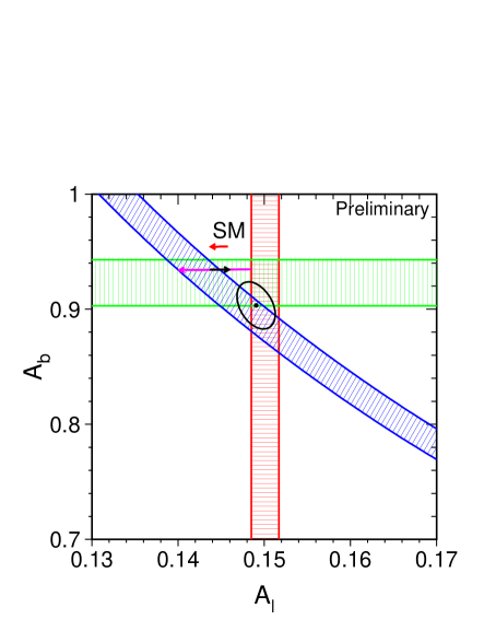
Figure 15.1: The measurements of the combined LEP+SLD ${\cal A}_{\ell}$ (vertical band), SLD ${\cal A}_{\mathrm{b}}$,${\cal A}_{\mathrm{c}}$ (horizontal bands) and LEP $A^{0,\,{\mathrm{b}}}_{\mathrm{FB}}$,$A^{0,\,{\mathrm{c}}}_{\mathrm{FB}}$ (diagonal bands), compared to the Standard Model expectations (arrows). The arrow pointing to the left shows the variation in the Standard Model prediction for $m_{\mathrm{H}}$ in the range $300^{+700}_{-186}$ GeV, and the arrow pointing to the right for $m_{\mathrm{t}}$ in the range $178.0\pm 4.3$ GeV. Varying the hadronic vacuum polarisation by $\Delta\alpha^{(5)}_{\mathrm{had}}(m_{\mathrm{Z}}^{2})=0.02761\pm 0.00036$ yields an additional uncertainty on the Standard Model prediction, oriented in direction of the Higgs-boson arrow and size corresponding to the top-quark arrow. Also shown is the 68% confidence level contour for the two asymmetry parameters resulting from the joint analyses. Although the $A^{0,\,{\mathrm{b}}}_{\mathrm{FB}}$ measurements prefer a high Higgs mass, the Standard Model fit to the full set of measurements prefers a low Higgs mass, for example because of the influence of ${\cal A}_{\ell}$.

15.2 The Effective Vector and Axial-Vector Coupling Constants

The partial widths of the $\mathrm{Z}$ into leptons and the lepton forward-backward asymmetries (Section 2), the $\tau$ polarisation and the $\tau$ polarisation asymmetry (Section 3) are combined to determine the effective vector and axial-vector couplings for $\rm e$, $\mu$ and $\tau$. The asymmetries (Equations (2.3) and (3.2)) determine the ratio $g_{\mathrm{V\ell}}/g_{\mathrm{A\ell}}$ (Equation (2.4)), while the leptonic partial widths determine the sum of the squares of the couplings:

$$\Gamma_{\ell\ell} = {{G_{\mathrm{F}}m_{\mathrm{Z}}^{3}}\over{6\pi\sqrt{2}}}(g_{\mathrm{V\ell}}^{2}+g_{\mathrm{A\ell}}^{2})(1+\delta^{QED}_{\ell})\,,$$ (15.1)

where $\delta^{QED}_{\ell}=3q^{2}_{\ell}\alpha(m_{\mathrm{Z}}^{2})/(4\pi)$, with $q_{\ell}$ denoting the electric charge of the lepton, accounts for final state photonic corrections. Corrections due to lepton masses, neglected in Equation 15.1, are taken into account for the results presented below.

The averaged results for the effective lepton couplings are given in Table 15.3 for both the LEP data alone as well as for the LEP and SLD measurements. Figure 15.2 shows the 68% probability contours in the $g_{\mathrm{A\ell}}$-$g_{\mathrm{V\ell}}$ plane for the individual lepton species. The signs of $g_{\mathrm{A\ell}}$ and $g_{\mathrm{V\ell}}$ are based on the convention $g_{\mathrm{Ae}}<0$. With this convention the signs of the couplings of all charged leptons follow from LEP data alone. The measured ratios of the $\rm e$, $\mu$ and $\tau$ couplings provide a test of lepton universality and are shown in Table 15.3. All values are consistent with lepton universality. The combined results assuming universality are also given in the table and are shown as a solid contour in Figure 15.2.

The neutrino couplings to the $\mathrm{Z}$ can be derived from the measured value of the invisible width of the $\mathrm{Z}$, $\Gamma_{\mathrm{inv}}$ (see Table 2.4), attributing it exclusively to the decay into three identical neutrino generations ($\Gamma_{\mathrm{inv}}=3\Gamma_{\nu\nu}$) and assuming $g_{{A}{\nu}}\equiv g_{{V}{\nu}}\equiv g_{\nu}$. The relative sign of $g_{\nu}$ is chosen to be in agreement with neutrino scattering data[267], resulting in $g_{\nu}=+0.50077\pm 0.00077$.

In addition, the couplings analysis is extended to include also the heavy-flavour measurements as presented in Section 5.3. Assuming neutral-current lepton universality, the effective coupling constants are determined jointly for leptons as well as for b and c quarks. QCD corrections, modifying Equation 15.1, are taken from the Standard Model, as is also done to obtain the quark pole asymmetries, see Section 5.2.3.

The results are also reported in Table 15.3 and shown in Figure 15.3. The deviation of the b-quark couplings from the Standard Model expectation is mainly caused by the combined value of ${\cal A}_{\mathrm{b}}$ being low as discussed in Section 15.1 and shown in Figure 15.1.

	Without Lepton Universality:
	LEP	LEP+SLD
$g_{\mathrm{Ae}}$	$-0.50112\pm 0.00035$	$-0.50111\pm 0.00035$
$g_{\mathrm{A\mu}}$	$-0.50115\pm 0.00056$	$-0.50120\pm 0.00054$
$g_{\mathrm{A\tau}}$	$-0.50204\pm 0.00064$	$-0.50204\pm 0.00064$
$g_{\mathrm{Ve}}$	$-0.0378\pm 0.0011$	$-0.03816\pm 0.00047$
$g_{\mathrm{V\mu}}$	$-0.0376\pm 0.0031$	$-0.0367\pm 0.0023$
$g_{\mathrm{V\tau}}$	$-0.0368\pm 0.0011$	$-0.0366\pm 0.0010$
	Ratios of couplings:
	LEP	LEP+SLD
$g_{\mathrm{A\mu}}/g_{\mathrm{Ae}}$	$1.0001\pm 0.0014$	$1.0002\pm 0.0014$
$g_{\mathrm{A\tau}}/g_{\mathrm{Ae}}$	$1.0018\pm 0.0015$	$1.0019\pm 0.0015$
$g_{\mathrm{V\mu}}/g_{\mathrm{Ve}}$	$0.995\pm 0.095$	$0.962\pm 0.063$
$g_{\mathrm{V\tau}}/g_{\mathrm{Ve}}$	$0.972\pm 0.041$	$0.958\pm 0.029$
	With Lepton Universality:
	LEP	LEP+SLD
$g_{\mathrm{A\ell}}$	$-0.50126\pm 0.00026$	$-0.50123\pm 0.00026$
$g_{\mathrm{V\ell}}$	$-0.03736\pm 0.00066$	$-0.03783\pm 0.00041$
$g_{\nu}$	$+0.50077\pm 0.00077$	$+0.50077\pm 0.00077$
	With Lepton Universality
	and Heavy Flavour Results:
	LEP	LEP+SLD
$g_{\mathrm{A\ell}}$	$-0.50126\pm 0.00026$	$-0.50125\pm 0.00026$
$g_{\mathrm{Ab}}$	$-0.5152\pm 0.0082$	$-0.5130\pm 0.0053$
$g_{\mathrm{Ac}}$	$+0.5016\pm 0.0081$	$+0.5036\pm 0.0054$
$g_{\mathrm{V\ell}}$	$-0.03735\pm 0.00066$	$-0.03757\pm 0.00037$
$g_{\mathrm{Vb}}$	$-0.321\pm 0.012$	$-0.3243\pm 0.0080$
$g_{\mathrm{Vc}}$	$+0.178\pm 0.011$	$+0.1874\pm 0.0069$

Table 15.3: Results for the effective vector and axial-vector couplings derived from the LEP data and the combined LEP and SLD data without and with the assumption of lepton universality. Note that the results, in particular for b quarks, are highly correlated.

Figure 15.2: Contours of 68% probability in the ($g_{\mathrm{V\ell}}$,$g_{\mathrm{A\ell}}$) plane from LEP and SLD measurements. The solid contour results from a fit to the LEP and SLD results assuming lepton universality. The shaded region corresponds to the Standard Model prediction for $m_{\mathrm{t}}=178.0\pm 4.3$ GeV and $m_{\mathrm{H}}=300^{+700}_{-186}\leavevmode\nobreak\ {\mathrm{Ge\kern-1.00006ptV}}$. The arrows point in the direction of increasing values of $m_{\mathrm{t}}$ and $m_{\mathrm{H}}$. Varying the hadronic vacuum polarisation by $\Delta\alpha^{(5)}_{\mathrm{had}}(m_{\mathrm{Z}}^{2})=0.02761\pm 0.00036$ yields an additional uncertainty on the Standard Model prediction indicated by the corresponding arrow.

Figure 15.3: Contours of 68.3, 95.5 and 99.5% probability in the ($g_{\mathrm{V}q}$,$g_{\mathrm{A}q}$) plane from LEP and SLD measurements for b and c quarks and assuming lepton universality. The dot corresponds to the Standard Model prediction for $m_{\mathrm{t}}=178.0\pm 4.3$ GeV, $m_{\mathrm{H}}=300^{+700}_{-186}\leavevmode\nobreak\ {\mathrm{Ge\kern-1.00006ptV}}$ and $\Delta\alpha^{(5)}_{\mathrm{had}}(m_{\mathrm{Z}}^{2})=0.02761\pm 0.00036$.

15.3 The Leptonic Effective Electroweak Mixing Angle $\sin^{2}\theta_{\mathrm{eff}}^{\mathrm{lept}}$

The asymmetry measurements from LEP and SLD can be combined into a single parameter, the effective electroweak mixing angle, $\sin^{2}\theta_{\mathrm{eff}}^{\mathrm{lept}}$, defined as:

$$\sin^{2}\theta_{\mathrm{eff}}^{\mathrm{lept}} \equiv \frac{1}{4}\left(1-\frac{g_{\mathrm{V\ell}}}{g_{\mathrm{A\ell}}}\right)\,,$$ (15.2)

without making strong model-specific assumptions.

For a combined average of $\sin^{2}\theta_{\mathrm{eff}}^{\mathrm{lept}}$ from $A^{0,\,\ell}_{\mathrm{FB}}$, ${\cal A}_{\tau}$ and ${\cal A}_{\mathrm{e}}$ only the assumption of lepton universality, already inherent in the definition of $\sin^{2}\theta_{\mathrm{eff}}^{\mathrm{lept}}$, is needed. Also the value derived from the measurements of ${\cal A}_{\ell}$ from SLD is given. We also include the hadronic forward-backward asymmetries, assuming the difference between $\sin^{2}\theta_{\mathrm{eff}}^{{\rm f}}$ for quarks and leptons to be given by the Standard Model. This is justified within the Standard Model as the hadronic asymmetries $A^{0,\,{\mathrm{b}}}_{\mathrm{FB}}$ and $A^{0,\,{\mathrm{c}}}_{\mathrm{FB}}$ have a reduced sensitivity to the small non-universal corrections specific to the quark vertex. The results of these determinations of $\sin^{2}\theta_{\mathrm{eff}}^{\mathrm{lept}}$ and their combination are shown in Table 15.4 and in Figure 15.4. The combinations based on the leptonic results plus ${\cal A}_{\ell}$(SLD) and on the hadronic forward-backward asymmetries differ by 2.8 standard deviations, caused by the two most precise measurements of $\sin^{2}\theta_{\mathrm{eff}}^{\mathrm{lept}}$, ${\cal A}_{\ell}$ (SLD) dominated by $A^{0}_{\mathrm{LR}}$, and $A^{0,\,{\mathrm{b}}}_{\mathrm{FB}}$ (LEP), likewise differing by 2.8 standard deviations. This is the same effect as discussed already in sections 15.1 and 15.2 and shown in Figures 15.1 and 15.3: the deviation in ${\cal A}_{\mathrm{b}}$ as extracted from $A^{0,\,{\mathrm{b}}}_{\mathrm{FB}}$ discussed above is reflected in the value of $\sin^{2}\theta_{\mathrm{eff}}^{\mathrm{lept}}$ extracted from $A^{0,\,{\mathrm{b}}}_{\mathrm{FB}}$ in this analysis.

	$\sin^{2}\theta_{\mathrm{eff}}^{\mathrm{lept}}$	Average by Group	Cumulative
		of Observations	Average	$\chi^{2}$/d.o.f.
$A^{0,\,\ell}_{\mathrm{FB}}$	$0.23099\pm 0.00053$
${\cal A}_{\ell}\leavevmode\nobreak\ ({\cal P}_{\tau})$	$0.23159\pm 0.00041$	$0.23137\pm 0.00033$		0.8/1
${\cal A}_{\ell}$ (SLD)	$0.23098\pm 0.00026$		$0.23113\pm 0.00021$	1.6/2
$A^{0,\,{\mathrm{b}}}_{\mathrm{FB}}$	$0.23210\pm 0.00030$
$A^{0,\,{\mathrm{c}}}_{\mathrm{FB}}$	$0.23223\pm 0.00081$
${\langle Q_{\mathrm{FB}}\rangle}$	$0.2324\pm 0.0012$	$0.23213\pm 0.00029$	$0.23147\pm 0.00017$	9.7/5

Table 15.4: Determinations of $\sin^{2}\theta_{\mathrm{eff}}^{\mathrm{lept}}$ from asymmetries. The second column lists the $\sin^{2}\theta_{\mathrm{eff}}^{\mathrm{lept}}$ values derived from the quantities listed in the first column. The third column contains the averages of these numbers by groups of observations, where the groups are separated by the horizontal lines. The fourth column shows the cumulative averages. The $\chi^{2}$ per degree of freedom for the cumulative averages is also given. The averages are performed including the small correlation between $A^{0,\,{\mathrm{b}}}_{\mathrm{FB}}$ and $A^{0,\,{\mathrm{c}}}_{\mathrm{FB}}$. The average of all six results has a probability of 8.4%.

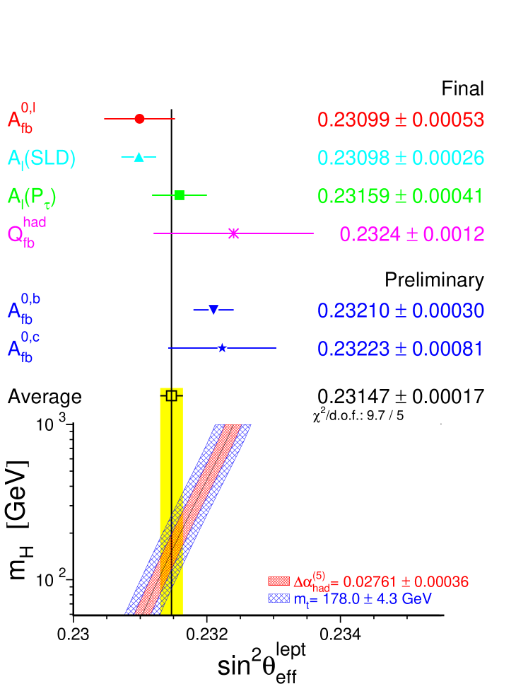
Figure 15.4: Comparison of several determinations of $\sin^{2}\theta_{\mathrm{eff}}^{\mathrm{lept}}$ from asymmetries. In the average, the small correlation between $A^{0,\,{\mathrm{b}}}_{\mathrm{FB}}$ and $A^{0,\,{\mathrm{c}}}_{\mathrm{FB}}$ is included. Also shown is the prediction of the Standard Model as a function of $m_{\mathrm{H}}$. The width of the Standard Model band is due to the uncertainties in $\Delta\alpha_{\mathrm{had}}^{(5)}(m_{\mathrm{Z}}^{2})$ (see Chapter 16), $m_{\mathrm{Z}}$ and $m_{\mathrm{t}}$. The total width of the band is the linear sum of these effects.

Chapter 16 Constraints on the Standard Model

Updates with respect to summer 2003:
Updated preliminary and published measurements as discussed in the previous chapters are taken into account, as well as new corrections in the measurement of atomic parity violation in Caesim and the new measurements of the electroweak mixing angle in Moller scattering. Newly calculated two-loop corrections in the SM calculation of the W-boson mass and the effective electroweak mixing angle are used for setting constraints on SM parameters.

16.1 Introduction

The precise electroweak measurements performed at LEP and SLC and elsewhere can be used to check the validity of the Standard Model and, within its framework, to infer valuable information about its fundamental parameters. The accuracy of the measurements makes them sensitive to the mass of the top quark $m_{\mathrm{t}}$, and to the mass of the Higgs boson $m_{\mathrm{H}}$ through loop corrections. While the leading $m_{\mathrm{t}}$ dependence is quadratic, the leading $m_{\mathrm{H}}$ dependence is logarithmic. Therefore, the inferred constraints on $m_{\mathrm{H}}$ are much weaker than those on $m_{\mathrm{t}}$.

16.2 Measurements

The LEP and SLD measurements used are summarised in Table 16.1. Also shown are the results of the Standard Model fit to all results.

The final results on the W-boson mass by UA2[268] and CDF[269, 270] and DØ[271] in Run-I, and the W-boson width by CDF[272] and DØ[273] in Run-I were recently combined based on a detailed treatment of common systematic uncertainties by the Tevatron Electroweak Working Group. The results are[274]: $m_{\mathrm{W}}=80452\pm 59\leavevmode\nobreak\ {\mathrm{Me\kern-1.00006ptV}}$, $\Gamma_{\mathrm{W}}=2102\pm 106\leavevmode\nobreak\ {\mathrm{Me\kern-1.00006ptV}}$, with a correlation of $-17.4\%$. Combining these results with the preliminary LEP-2 measurements as presented in Chapter 14, the new preliminary world averages used in the following analyses are:

$$m_{\mathrm{W}} = 80.425\pm 0.034\leavevmode\nobreak\ {\mathrm{Ge\kern-1.00006ptV}}$$ (16.1)

$$\Gamma_{\mathrm{W}} = 2.133\pm 0.069\leavevmode\nobreak\ {\mathrm{Ge\kern-1.00006ptV}}\,$$ (16.2)

with a correlation of $-6.7\%$.

For the mass of the top quark, $m_{\mathrm{t}}$, the published results from CDF [275] and DØ [276], including the recently published precise measurement from the DØ collaboration, are combined by the Tevatron Electroweak Working Group [277], with the result $m_{\mathrm{t}}=178.0\pm 4.3\leavevmode\nobreak\ {\mathrm{Ge\kern-1.00006ptV}}$.

In addition, the final result of the NuTeV collaboration on neutrino-nucleon neutral to charged current cross section ratios [278], the measurements of atomic parity violation in caesium[279, 280], with the numerical result[281] taken from a recently published revised analysis of QED radiative corrections applied to the raw measurement, and the effective electroweak mixing angle measured in Moller scattering [282], are included in some of the analyses shown below, see Table 16.2. Although the $\nu{\cal N}$ result is quoted in terms of $\sin^{2}\theta_{\mathrm{W}}=1-m_{\mathrm{W}}^{2}/m_{\mathrm{Z}}^{2}=0.2277\pm 0.0016$, radiative corrections result in small $m_{\mathrm{t}}$ and $m_{\mathrm{H}}$ dependences that are included in the fit. Note that the NuTeV result in terms of the on-shell electroweak mixing angle is about 3 standard deviations higher than the expectation.

An additional input parameter, not shown in the table, is the Fermi constant $G_{F}$, determined from the $\mu$ lifetime, $G_{F}=1.16637(1)\cdot 10^{-5}{\mathrm{Ge\kern-1.00006ptV}}^{-2}$[283]. The relative error of $G_{F}$ is comparable to that of $m_{\mathrm{Z}}$; both errors have negligible effects on the fit results.

		Measurement with	Systematic	Standard	Pull
		Total Error	Error	Model fit
	$\Delta\alpha^{(5)}_{\mathrm{had}}(m_{\mathrm{Z}}^{2})$[284]	$0.02761\pm 0.00036$	0.00035	0.02767	$-0.2$
a)	LEP
	line-shape and
	lepton asymmetries:
	$m_{\mathrm{Z}}$ [GeV]	$91.1875\pm 0.0021\phantom{0}$	(a)0.0017	91.1875	$0.0$
	$\Gamma_{\mathrm{Z}}$ [GeV]	$2.4952\pm 0.0023\phantom{0}$	(a)0.0012	2.4966	$-0.6$
	$\sigma_{\mathrm{h}}^{0}$ [nb]	$41.540\pm 0.037\phantom{00}$	(b)0.028	41.481	$1.6$
	$R^{0}_{\ell}$	$20.767\pm 0.025\phantom{00}$	(b)0.007	20.739	$1.1$
	$A^{0,\,\ell}_{\mathrm{FB}}$	$0.0171\pm 0.0010\phantom{0}$	(b)0.0003	0.0165	$0.7$
	+ correlation matrix Table 2.3
	$\tau$ polarisation:
	${\cal A}_{\ell}\leavevmode\nobreak\ ({\cal P}_{\tau})$	$0.1465\pm 0.0033\phantom{0}$	0.0016	0.1483	$-0.6$
	$\mathrm{q\overline{q}}$ charge asymmetry:
	$\sin^{2}\theta_{\mathrm{eff}}^{\mathrm{lept}}({Q^{\mathrm{had}}_{\mathrm{FB}}})$	$0.2324\pm 0.0012\phantom{0}$	0.0010	0.2314	$0.9$
b)	SLD[285]
	${\cal A}_{\ell}$ (SLD)	$0.1513\pm 0.0021\phantom{0}$	0.0010	0.1483	$1.4$
c)	LEP and SLD Heavy Flavour
	$R_{\mathrm{b}}^{0}{}$	$0.21630\pm 0.00066$	0.00050	0.21562	$1.0$
	$R_{\mathrm{c}}^{0}{}$	$0.1723\pm 0.0031\phantom{0}$	0.0019	0.1723	$0.0$
	$A^{0,\,{\mathrm{b}}}_{\mathrm{FB}}{}$	$0.0998\pm 0.0017\phantom{0}$	0.0009	0.1040	$-2.4$
	$A^{0,\,{\mathrm{c}}}_{\mathrm{FB}}{}$	$0.0706\pm 0.0035\phantom{0}$	0.0017	0.0744	$-1.1$
	${\cal A}_{\mathrm{b}}$	$0.923\pm 0.020\phantom{00}$	0.013	0.935	$-0.6$
	${\cal A}_{\mathrm{c}}$	$0.670\pm 0.026\phantom{00}$	0.015	0.668	$0.1$
	+ correlation matrix Table 5.3
d)	Additional
	$m_{\mathrm{W}}$ [GeV] ($\mathrm{p\overline{p}}$ and LEP-2)	$80.425\pm 0.034\phantom{00}$		80.394	$0.9$
	$\Gamma_{\mathrm{W}}$ [GeV] ($\mathrm{p\overline{p}}$ and LEP-2)	$2.133\pm 0.069\phantom{00}$		2.093	$0.6$
	$m_{\mathrm{t}}$ [GeV] ($\mathrm{p\overline{p}}$[277])	$178.0\pm 4.3\phantom{00}\phantom{00}$	3.3	178.1	$0.0$

Table 16.1: Summary of high-$Q^{2}$ measurements included in the combined analysis of Standard Model parameters. Section a) summarises LEP averages, Section b) SLD results ($\sin^{2}\theta_{\mathrm{eff}}^{\mathrm{lept}}$ includes $A_{\mathrm{LR}}$ and the polarised lepton asymmetries), Section c) the LEP and SLD heavy flavour results and Section d) electroweak measurements from $\mathrm{p\overline{p}}$ colliders and LEP-2. The total errors in column 2 include the systematic errors listed in column 3. Although the systematic errors include both correlated and uncorrelated sources, the determination of the systematic part of each error is approximate. The Standard Model results in column 4 and the pulls (difference between measurement and fit in units of the total measurement error) in column 5 are derived from the Standard Model fit including all data (Table 16.3, column 5) with the Higgs mass treated as a free parameter.
^(a)The systematic errors on $m_{\mathrm{Z}}$ and $\Gamma_{\mathrm{Z}}$ contain the errors arising from the uncertainties in the LEP energy only.
^(b)Only common systematic errors are indicated.

16.3 Theoretical and Parametric Uncertainties

Detailed studies of the theoretical uncertainties in the Standard Model predictions due to missing higher-order electroweak corrections and their interplay with QCD corrections are carried out by the working group on ‘Precision calculations for the $\mathrm{Z}$ resonance’[286], and more recently in [15]. Theoretical uncertainties are evaluated by comparing different but, within our present knowledge, equivalent treatments of aspects such as resummation techniques, momentum transfer scales for vertex corrections and factorisation schemes. The effects of these theoretical uncertainties are reduced by the inclusion of higher-order corrections[287, 288] in the electroweak libraries[289].

Recently, the complete (fermionic and bosonic) two-loop corrections for the calculation of $m_{\mathrm{W}}$ [290], and the complete fermionic two-loop corrections for the calculation of $\sin^{2}\theta_{\mathrm{eff}}^{\mathrm{lept}}$ [291] have been calculated. Including three-loop top-quark contributions to the $\rho$ parameter in the limit of large $m_{\mathrm{t}}$ [292], efficient routines for evaluating these corrections have been implemented in the new version 6.40 of the semi-analytical program ZFITTER. The remaining theoretical uncertainties are estimated to be $4\leavevmode\nobreak\ {\mathrm{Me\kern-1.00006ptV}}$ on $m_{\mathrm{W}}$ and 0.000049 on $\sin^{2}\theta_{\mathrm{eff}}^{\mathrm{lept}}$. The latter uncertainty dominates the theoretical uncertainty in SM fits and the extraction of constraints on the mass of the Higgs boson presented below. For a complete picture, the complete two-loop calculation for the partial Z decay widths should be calculated.

The use of the QCD corrections[288] increases the value of $\alpha_{\mathrm{S}}(m_{\mathrm{Z}}^{2})$ by 0.001, as expected. The effects of missing higher-order QCD corrections on $\alpha_{\mathrm{S}}(m_{\mathrm{Z}}^{2})$ covers missing higher-order electroweak corrections and uncertainties in the interplay of electroweak and QCD corrections and is estimated to be at least 0.002 [293]. A discussion of theoretical uncertainties in the determination of $\alpha_{\mathrm{S}}$ can be found in References 286 and 293. The determination of the size of remaining theoretical uncertainties is under continued study.

The theoretical errors discussed above are not included in the results presented in Table 16.3. At present the impact of theoretical uncertainties on the determination of Standard Model parameters from the precise electroweak measurements is small compared to the error due to the uncertainty in the value of $\alpha(m_{\mathrm{Z}}^{2})$, which is included in the results.

The uncertainty in $\alpha(m_{\mathrm{Z}}^{2})$ arises from the contribution of light quarks to the photon vacuum polarisation ($\Delta\alpha_{\mathrm{had}}^{(5)}(m_{\mathrm{Z}}^{2})$):

$$\alpha(m_{\mathrm{Z}}^{2})=\frac{\alpha(0)}{1-\Delta\alpha_{\ell}(m_{\mathrm{Z}}^{2})-\Delta\alpha_{\mathrm{had}}^{(5)}(m_{\mathrm{Z}}^{2})-\Delta\alpha_{\mathrm{top}}(m_{\mathrm{Z}}^{2})}\,,$$ (16.3)

where $\alpha(0)=1/137.036$. The top contribution, $-0.00007(1)$, depends on the mass of the top quark, and is therefore determined inside the electroweak libraries[289]. The leptonic contribution is calculated to third order[294] to be $0.03150$, with negligible uncertainty.

For the hadronic contribution, we no longer use the value $0.02804\pm 0.00065$[295], but rather the new evaluation $0.02761\pm 0.0036$ [284] which takes into account the recently published results on electron-positron annihilations into hadrons at low centre-of-mass energies by the BES collaboration [296]. This reduced uncertainty still causes an error of 0.00013 on the Standard Model prediction of $\sin^{2}\theta_{\mathrm{eff}}^{\mathrm{lept}}$, and errors of 0.2 GeV and 0.1 on the fitted values of $m_{\mathrm{t}}$ and $\log(m_{\mathrm{H}})$, included in the results presented below. The effect on the Standard Model prediction for $\Gamma_{\ell\ell}$ is negligible. The $\alpha_{\mathrm{S}}(m_{\mathrm{Z}}^{2})$ values for the Standard Model fits presented here are stable against a variation of $\alpha(m_{\mathrm{Z}}^{2})$ in the interval quoted. As presented at the ICHEP04 conference, the effect of the revised published results from CMD-2 and of new results from KLOE on the hadronic cross section at low centre-of-mass energies on $\Delta\alpha^{(5)}_{\mathrm{had}}(m_{\mathrm{Z}}^{2})$ largely cancel each other so that the numerical value quoted above is still valid [297].

There are also several evaluations of $\Delta\alpha^{(5)}_{\mathrm{had}}(m_{\mathrm{Z}}^{2})$[298, 299, 300, 301, 302, 303, 304, 305, 306, 307, 308] which are more theory-driven. One of the most recent of these (Reference 308) also includes the new results from BES, yielding $0.02749\pm 0.00012$. To show the effects of the uncertainty of $\alpha(m_{\mathrm{Z}}^{2})$, we also use this evaluation of the hadronic vacuum polarisation. Note that all these evaluations obtain values for $\Delta\alpha^{(5)}_{\mathrm{had}}(m_{\mathrm{Z}}^{2})$ consistently lower than - but still in agreement with - the old value of $0.02804\pm 0.00065$.

16.4 Selected Results

Figure 16.1 shows a comparison of the leptonic partial width from LEP (Table 2.4) and the effective electroweak mixing angle from asymmetries measured at LEP and SLD (Table 15.4), with the Standard Model. Good agreement with the Standard Model prediction is observed. The point with the arrow indicates the prediction if among the electroweak radiative corrections only the photon vacuum polarisation is included, which shows that LEP+SLD data are sensitive to non-trivial electroweak corrections. Note that the error due to the uncertainty on $\alpha(m_{\mathrm{Z}}^{2})$ (shown as the length of the arrow) is not much smaller than the experimental error on $\sin^{2}\theta_{\mathrm{eff}}^{\mathrm{lept}}$ from LEP and SLD. This underlines the continued importance of a precise measurement of $\sigma(\mathrm{e^{+}e^{-}\rightarrow hadrons})$ at low centre-of-mass energies.

Of the measurements given in Table 16.1, $R^{0}_{\ell}$ is one of the most sensitive to QCD corrections. For $m_{\mathrm{Z}}=91.1875$ GeV, and imposing $m_{\mathrm{t}}=178.0\pm 4.3$ GeV as a constraint, $\alpha_{\mathrm{S}}=0.1226\pm 0.0038$ is obtained. Alternatively, $\sigma_{\ell}^{0}$ (see Table 2.4) which has higher sensitivity to QCD corrections and less dependence on $m_{\mathrm{H}}$ yields: $\alpha_{\mathrm{S}}=0.1183\pm 0.0030$. Typical errors arising from the variation of $m_{\mathrm{H}}$ between $100\leavevmode\nobreak\ {\mathrm{Ge\kern-1.00006ptV}}$ and $200\leavevmode\nobreak\ {\mathrm{Ge\kern-1.00006ptV}}$ are of the order of $0.001$, somewhat smaller for $\sigma_{\ell}^{0}$. These results on $\alpha_{\mathrm{S}}$, as well as those reported in the next section, are in very good agreement with recently determined world averages ($\alpha_{\mathrm{S}}(m_{\mathrm{Z}}^{2})=0.118\pm 0.002$[309], or $\alpha_{\mathrm{S}}(m_{\mathrm{Z}}^{2})=0.1178\pm 0.0033$ based solely on NNLO QCD results excluding the LEP lineshape results and accounting for correlated errors[310]).

16.5 Standard Model Analyses

In the following, several different Standard Model fits to the data reported in Table 16.3 are discussed. The $\chi^{2}$ minimisation is performed with the program MINUIT [136], and the predictions are calculated with TOPAZ0 [311] and ZFITTER [37]. The somewhat increased $\chi^{2}$/d.o.f. for all of these fits is caused by the same effect as discussed in the previous chapter, namely the large dispersion in the values of the leptonic effective electroweak mixing angle measured through the various asymmetries. For the analyses presented here, this dispersion is interpreted as a fluctuation in one or more of the input measurements, and thus we neither modify nor exclude any of them. A further drastic increase in $\chi^{2}$/d.o.f. is observed when the NuTeV result on $\sin^{2}\theta_{\mathrm{W}}$ is included in the analysis.

To test the agreement between the LEP data and the Standard Model, a fit to the LEP data (including the LEP-II $m_{\mathrm{W}}$ and $\Gamma_{\mathrm{W}}$ determinations) leaving the top quark mass and the Higgs mass as free parameters is performed. The result is shown in Table 16.3, column 1. This fit shows that the LEP data predicts the top mass in good agreement with the direct measurements. In addition, the data prefer an intermediate Higgs-boson mass, albeit with very large errors. The strongly asymmetric errors on $m_{\mathrm{H}}$ are due to the fact that to first order, the radiative corrections in the Standard Model are proportional to $\log(m_{\mathrm{H}})$.

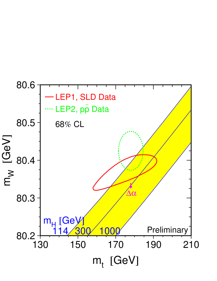
Figure 16.2: The comparison of the indirect measurements of $m_{\mathrm{W}}$ and $m_{\mathrm{t}}$ (LEP-I+ SLD data) (solid contour) and the direct measurements ($\mathrm{p\overline{p}}$ colliders and LEP-II data) (dashed contour). In both cases the 68% CL contours are plotted. Also shown is the Standard Model relationship for the masses as a function of the Higgs mass. The arrow labelled $\Delta\alpha$ shows the variation of this relation if $\alpha(m_{\mathrm{Z}}^{2})$ is changed by one standard deviation. This variation gives an additional uncertainty to the Standard Model band shown in the figure.

The data can also be used within the Standard Model to determine the top quark and W masses indirectly, which can be compared to the direct measurements performed at the $\mathrm{p\overline{p}}$ colliders and LEP-II. In the second fit, all LEP and SLD results in Table 16.1, except the measurements of $m_{\mathrm{W}}$ and $\Gamma_{\mathrm{W}}$, are used. The results are shown in column 2 of Table 16.3. The indirect measurements of $m_{\mathrm{W}}$ and $m_{\mathrm{t}}$ from this data sample are shown in Figure 16.2, compared with the direct measurements. Also shown are the Standard Model predictions for Higgs masses between 114 and 1000 GeV. As can be seen in the figure, the indirect and direct measurements of $m_{\mathrm{W}}$ and $m_{\mathrm{t}}$ are in good agreement, and both sets prefer a low value of the Higgs mass.

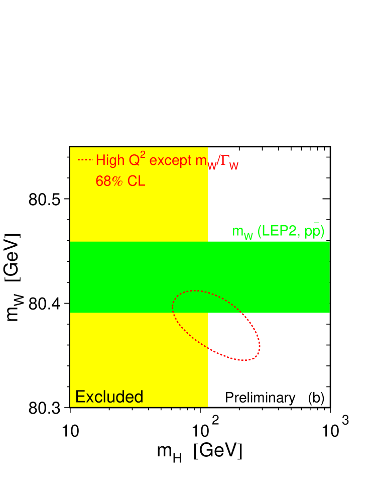
Figure 16.3: The 68% confidence level contour in $m_{\mathrm{W}}$ and $m_{\mathrm{H}}$ for the fit to all data except the direct measurement of $m_{\mathrm{W}}$, indicated by the shaded horizontal band of $\pm 1$ sigma width. The vertical band shows the 95% CL exclusion limit on $m_{\mathrm{H}}$ from the direct search.

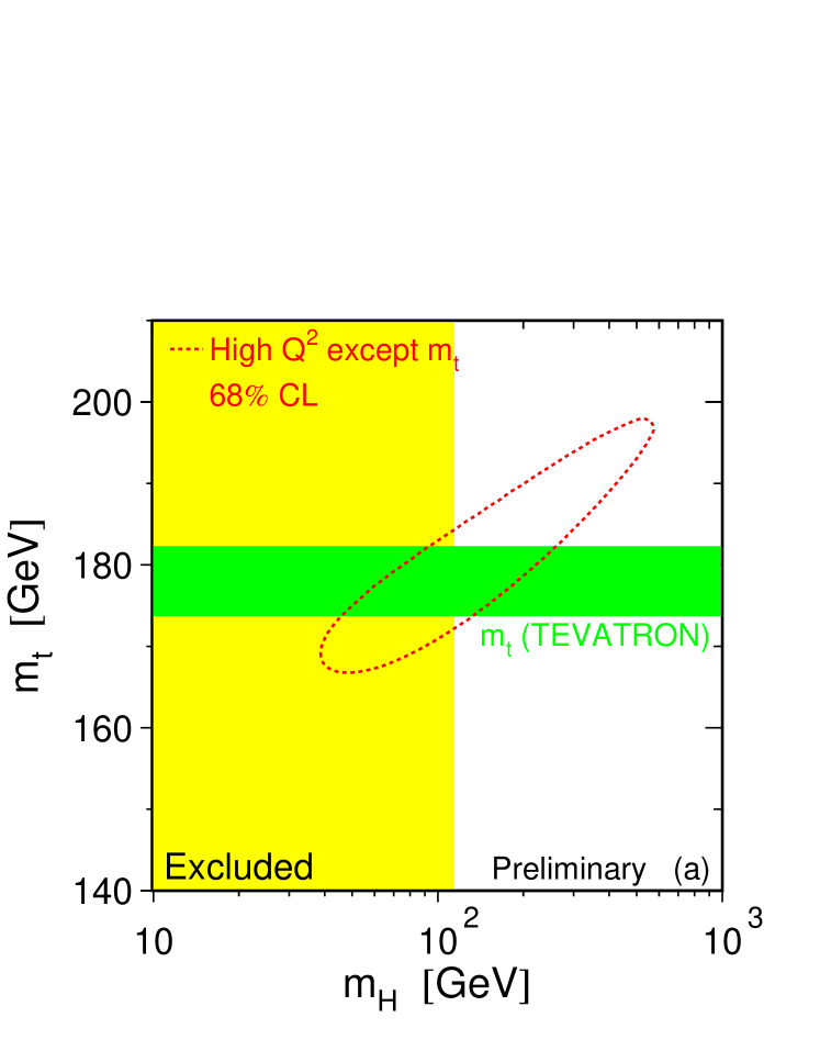
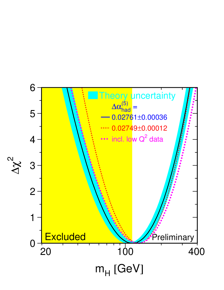
Figure 16.4: The 68% confidence level contour in $m_{\mathrm{t}}$ and $m_{\mathrm{H}}$ for the fit to all data except the direct measurement of $m_{\mathrm{t}}$, indicated by the shaded horizontal band of $\pm 1$ sigma width. The vertical band shows the 95% CL exclusion limit on $m_{\mathrm{H}}$ from the direct search.

For the third fit, the direct $m_{\mathrm{t}}$ measurement is used to obtain the best indirect determination of $m_{\mathrm{W}}$. The result is shown in column 3 of Table 16.3 and in Figure 16.3. Also here, the indirect determination of W boson mass $80.379\pm 0.023$ GeV is in good agreement with the combination of direct measurements from LEP-II and $\mathrm{p\overline{p}}$ colliders of $m_{\mathrm{W}}=80.425\pm 0.034$ GeV. For the next fit, (column 4 of Table 16.3 and Figure 16.4), the direct $m_{\mathrm{W}}$ and $\Gamma_{\mathrm{W}}$ measurements from LEP and $\mathrm{p\overline{p}}$ colliders are included to obtain $m_{\mathrm{t}}=179^{+12}_{-9}$ GeV, in very good agreement with the direct measurement of $m_{\mathrm{t}}=178.0\pm 4.3$ GeV. Compared to the second fit, the error on $\log m_{\mathrm{H}}$ increases due to effects from higher-order terms.

Finally, the best constraints on $m_{\mathrm{H}}$ are obtained when all high-$Q^{2}$ measurements are used in the fit. The results of this fit are shown in column 5 of Table 16.3. The predictions of this fit for observables measured in high-$Q^{2}$ and low-$Q^{2}$ reactions are listed in Tables 16.1 and 16.2, respectively. In Figure 16.5 the observed value of $\Delta\chi^{2}\equiv\chi^{2}-\chi^{2}_{\mathrm{min}}$ as a function of $m_{\mathrm{H}}$ is plotted for the fit including all data. The solid curve is the result using ZFITTER, and corresponds to the last column of Table 16.3. The shaded band represents the uncertainty due to uncalculated higher-order corrections, as estimated by TOPAZ0 and ZFITTER.

The 95% confidence level upper limit on $m_{\mathrm{H}}$ (taking the band into account) is 260 GeV. The 95% C.L. lower limit on $m_{\mathrm{H}}$ of 114.4 GeV obtained from direct searches[312] is not used in the determination of this limit. Also shown is the result (dashed curve) obtained when using $\Delta\alpha^{(5)}_{\mathrm{had}}(m_{\mathrm{Z}}^{2})$ of Reference 306.

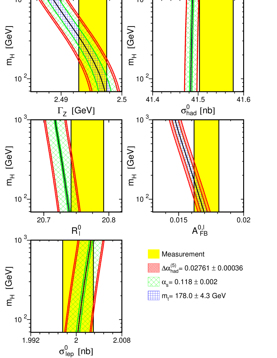
Figure 16.6: Comparison of LEP-I measurements with the Standard Model prediction as a function of $m_{\mathrm{H}}$. The measurement with its error is shown as the vertical band. The width of the Standard Model band is due to the uncertainties in $\Delta\alpha^{(5)}_{\mathrm{had}}(m_{\mathrm{Z}}^{2})$, $\alpha_{\mathrm{S}}(m_{\mathrm{Z}}^{2})$ and $m_{\mathrm{t}}$. The total width of the band is the linear sum of these effects.

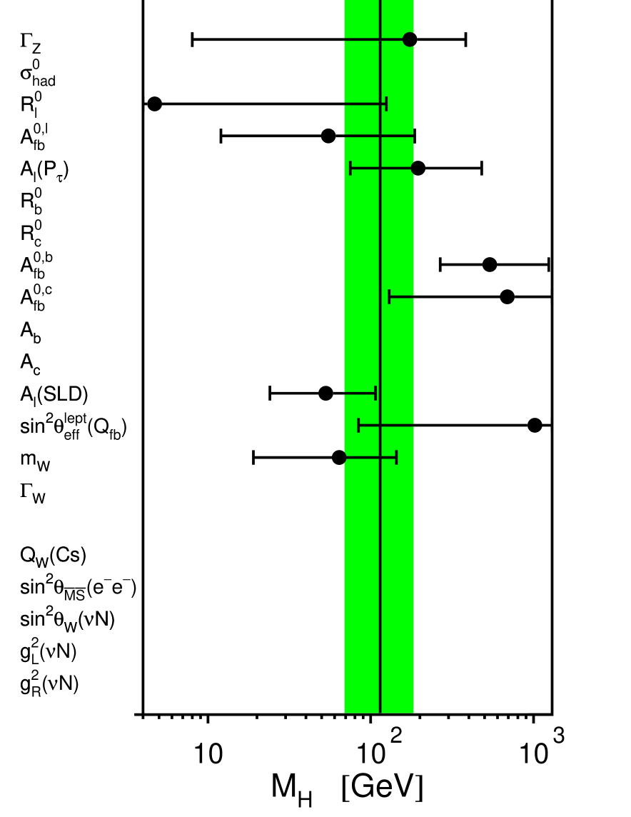
Figure 16.10: Constraints on the mass of the Higgs boson from each pseudo-observable. The Higgs-boson mass and its 68% CL uncertainty is obtained from a five-parameter Standard Model fit to the observable, constraining $\Delta\alpha^{(5)}_{\mathrm{had}}(m_{\mathrm{Z}}^{2})=0.02761\pm 0.00036$, $\alpha_{\mathrm{S}}(m_{\mathrm{Z}}^{2})=0.118\pm 0.002$, $m_{\mathrm{Z}}=91.1875\pm 0.0021\leavevmode\nobreak\ {\mathrm{Ge\kern-1.00006ptV}}$ and $m_{\mathrm{t}}=178.0\pm 4.3\leavevmode\nobreak\ {\mathrm{Ge\kern-1.00006ptV}}$. Because of these four common constraints the resulting Higgs-boson mass values cannot be combined. The shaded band denotes the overall constraint on the mass of the Higgs boson derived from all pseudo-observables including the above four Standard Model parameters as reported in the last column of Table 16.3.

In Figures 16.6 to 16.9 the sensitivity of the LEP and SLD measurements to the Higgs mass is shown. Besides the measurement of the W mass, the most sensitive measurements are the asymmetries, i.e., $\sin^{2}\theta_{\mathrm{eff}}^{\mathrm{lept}}$. A reduced uncertainty for the value of $\alpha(m_{\mathrm{Z}}^{2})$ would therefore result in an improved constraint on $\log m_{\mathrm{H}}$ and thus $m_{\mathrm{H}}$, as already shown in Figures 16.1 and 16.5. Given the constraints on the other four Standard Model input parameters, each observable is equivalent to a constraint on the mass of the Standard Model Higgs boson. The constraints on the mass of the Standard Model Higgs boson resulting from each observable are compared in Figure 16.10. For vey low Higgs-masses, these constraints are qualitative only as the effects of real Higgs-strahlung, neither included in the experimental analyses nor in the SM calculations of expectations, may then become sizeable [313].

		Measurement with	Systematic	Standard	Pull
		Total Error	Error	Model fit
	$Q_{\mathrm{W}}(\mathrm{Cs})$ [314]	$-72.74\pm 0.46\phantom{00}\phantom{0}$	0.36	$-72.93\phantom{0}\phantom{00}$	$0.4$
	$\sin^{2}\theta_{\overline{MS}}(m_{\mathrm{Z}})$ [282]	$0.2330\pm 0.0016\phantom{0}$	0.0012	0.2311	$1.2$
	$\sin^{2}\theta_{\mathrm{W}}$ ($\nu{\cal N}$[278])	$0.2277\pm 0.0016\phantom{0}$	0.0009	0.2227	$3.1$

Table 16.2: Summary of measurements performed in low-$Q^{2}$ reactions, namely atomic parity violation, $E^{-}e^{-}$ Moller scattering and neutrino-nucleon scattering. The total errors in column 2 include the systematic errors listed in column 3. The Standard Model results in column 4 and the pulls (difference between measurement and fit in units of the total measurement error) in column 5 are derived from the Standard Model fit including all high-$Q^{2}$ data (Table 16.3, column 5) with the Higgs mass treated as a free parameter.

	- 1 -	- 2 -	- 3 -	- 4 -	- 5 -
	LEP including	all Z-pole	all Z-pole data	all Z-pole data	all Z-pole data
	LEP-II $m_{\mathrm{W}}$, $\Gamma_{\mathrm{W}}$	data	plus $m_{\mathrm{t}}$	plus $m_{\mathrm{W}}$, $\Gamma_{\mathrm{W}}$	plus $m_{\mathrm{t}},m_{\mathrm{W}},\Gamma_{\mathrm{W}}$
$m_{\mathrm{t}}$ [GeV]	$180^{+14}_{-11}$	$172^{+13}_{-9}$	$177.3^{+4.1}_{-4.1}$	$179^{+12}_{-9}$	$178.2^{+4.0}_{-3.9}$
$m_{\mathrm{H}}$ [GeV]	$214^{+400}_{-129}$	$92^{+150}_{-48}$	$136^{+88}_{-55}$	$124^{+207}_{-69}$	$114^{+69}_{-45}$
$\log(m_{\mathrm{H}}/{\mathrm{Ge\kern-1.00006ptV}})$	$2.33^{+0.46}_{-0.40}$	$1.96^{+0.42}_{-0.32}$	$2.13^{+0.22}_{-0.23}$	$2.09^{+0.43}_{-0.35}$	$2.06^{+0.20}_{-0.21}$
$\alpha_{\mathrm{S}}(m_{\mathrm{Z}}^{2})$	$0.1199\pm 0.0030$	$0.1187\pm 0.0027$	$0.1190\pm 0.0027$	$0.1187\pm 0.0028$	$0.1186\pm 0.0027$
$\chi^{2}$/d.o.f. ($P$)	$11.3/9\leavevmode\nobreak\ (25\%)$	$13.9/10\leavevmode\nobreak\ (18\%)$	$14.1/11\leavevmode\nobreak\ (23\%)$	$15.8/12\leavevmode\nobreak\ (20\%)$	$15.8/14\leavevmode\nobreak\ (26\%)$
$\sin^{2}\theta_{\mathrm{eff}}^{\mathrm{lept}}$	$\phantom{0}0.23160$	$\phantom{0}0.23144$	$\phantom{0}0.23144$	$\phantom{0}0.23136$	$\phantom{0}0.23136$
	$\pm 0.00017$	$\pm 0.00016$	$\pm 0.00016$	$\pm 0.00015$	$\pm 0.00014$
$\sin^{2}\theta_{\mathrm{W}}$	$\phantom{0}0.22322$	$\phantom{0}0.22322$	$\phantom{0}0.22300$	$\phantom{0}0.22269$	$\phantom{0}0.22272$
	$\pm 0.00051$	$\pm 0.00062$	$\pm 0.00044$	$\pm 0.00044$	$\pm 0.00036$
$m_{\mathrm{W}}$ [GeV]	$80.368\pm 0.026$	$80.368\pm 0.032$	$80.379\pm 0.023$	$80.395\pm 0.023$	$80.394\pm 0.019$

Table 16.3: Results of the fits to: (1) LEP data alone, (2) all Z-pole data (LEP-1 and SLD), (3) all Z-pole data plus direct $m_{\mathrm{t}}$ determinations, (4) all Z-pole data plus direct $m_{\mathrm{W}}$ and direct $\Gamma_{\mathrm{W}}$ determinations, (5) all Z-pole data plus direct $m_{\mathrm{t}},m_{\mathrm{W}},\Gamma_{\mathrm{W}}$ determinations (i.e., all high-$Q^{2}$ results). As the sensitivity to $m_{\mathrm{H}}$ is logarithmic, both $m_{\mathrm{H}}$ as well as $\log(m_{\mathrm{H}}/{\mathrm{Ge\kern-1.00006ptV}})$ are quoted. The bottom part of the table lists derived results for $\sin^{2}\theta_{\mathrm{eff}}^{\mathrm{lept}}$, $\sin^{2}\theta_{\mathrm{W}}$ and $m_{\mathrm{W}}$. See text for a discussion of theoretical errors not included in the errors above.

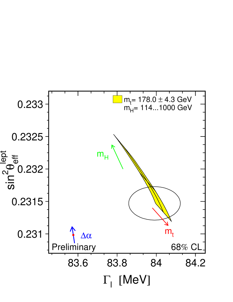
Figure 16.1: LEP-I+SLD measurements of $\sin^{2}\theta_{\mathrm{eff}}^{\mathrm{lept}}$ (Table 15.4) and $\Gamma_{\ell\ell}$ (Table 2.4) and the Standard Model prediction. The point shows the predictions if among the electroweak radiative corrections only the photon vacuum polarisation is included. The corresponding arrow shows variation of this prediction if $\alpha(m_{\mathrm{Z}}^{2})$ is changed by one standard deviation. This variation gives an additional uncertainty to the Standard Model prediction shown in the figure.

Figure 16.5: $\Delta\chi^{2}=\chi^{2}-\chi^{2}_{min}$ vs. $m_{\mathrm{H}}$ curve. The line is the result of the fit using all data (last column of Table 16.3); the band represents an estimate of the theoretical error due to missing higher order corrections. The vertical band shows the 95% CL exclusion limit on $m_{\mathrm{H}}$ from the direct search. The dashed curve is the result obtained using the evaluation of $\Delta\alpha^{(5)}_{\mathrm{had}}(m_{\mathrm{Z}}^{2})$ from Reference 308.

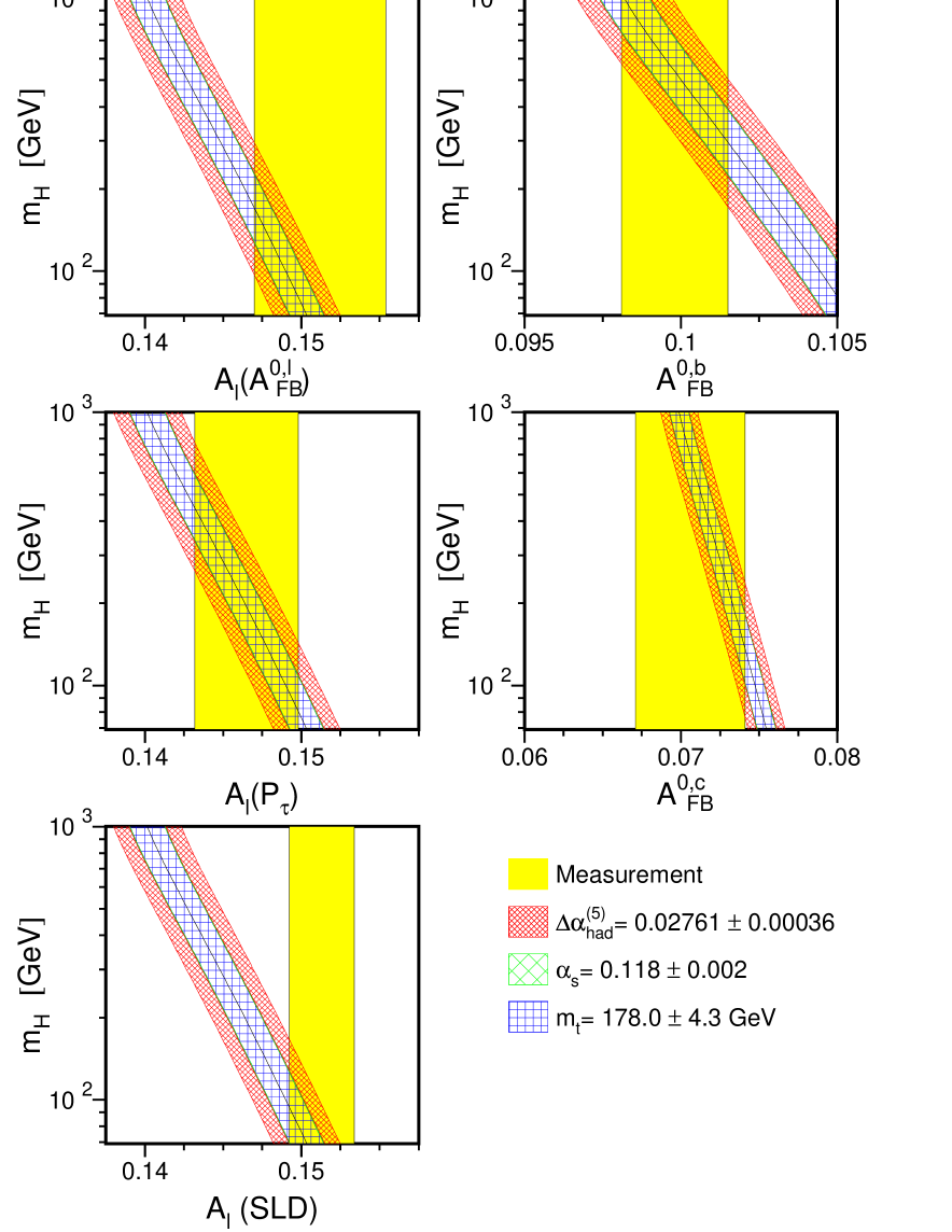
Figure 16.7: Comparison of LEP-I measurements with the Standard Model prediction as a function of $m_{\mathrm{H}}$. The measurement with its error is shown as the vertical band. The width of the Standard Model band is due to the uncertainties in $\Delta\alpha^{(5)}_{\mathrm{had}}(m_{\mathrm{Z}}^{2})$, $\alpha_{\mathrm{S}}(m_{\mathrm{Z}}^{2})$ and $m_{\mathrm{t}}$. The total width of the band is the linear sum of these effects. Also shown is the comparison of the SLD measurement of ${\cal A}_{\ell}$, dominated by $A^{0}_{\mathrm{LR}}$, with the Standard Model.

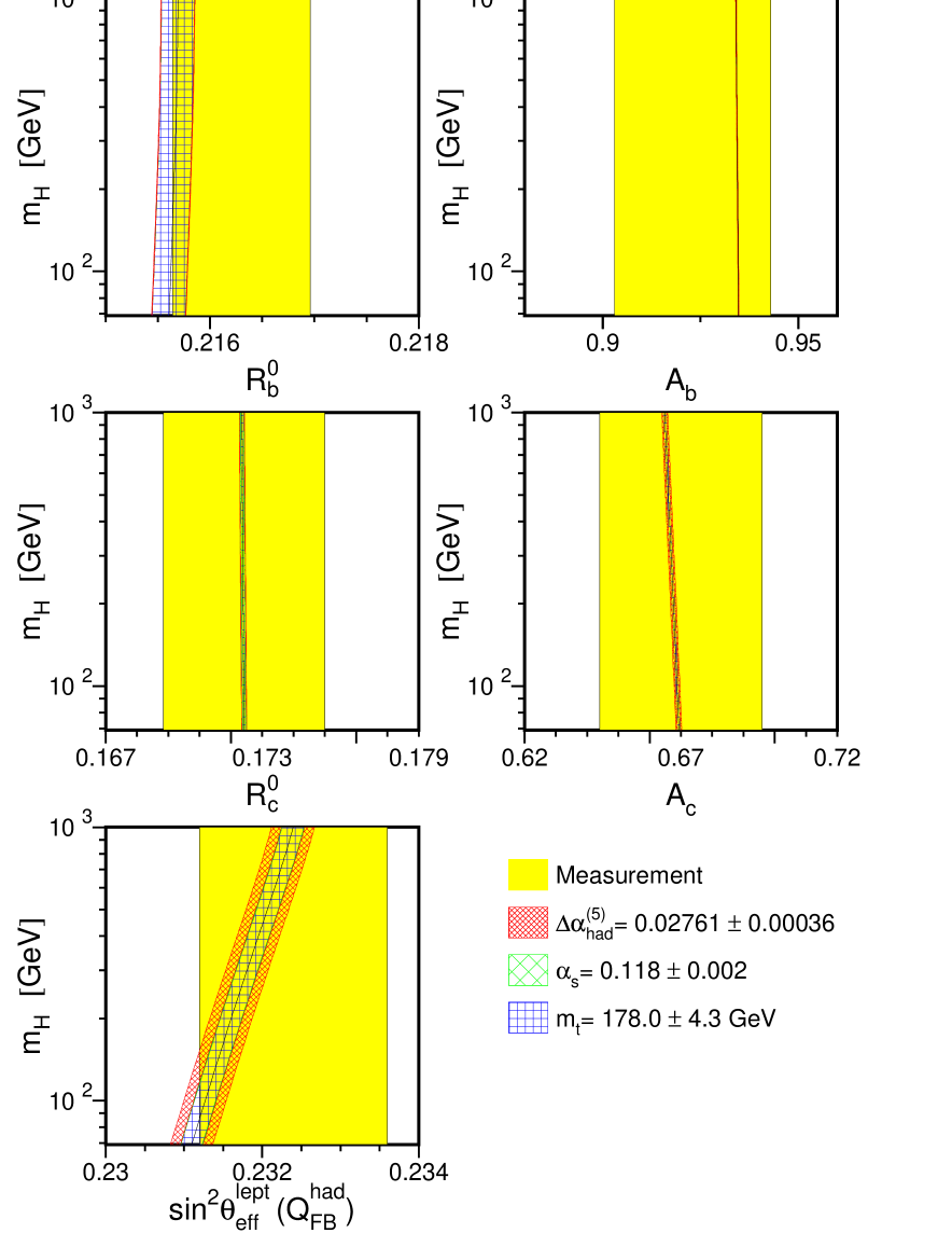
Figure 16.8: Comparison of LEP-I and SLD heavy-flavour measurements with the Standard Model prediction as a function of $m_{\mathrm{H}}$. The measurement with its error is shown as the vertical band. The width of the Standard Model band is due to the uncertainties in $\Delta\alpha^{(5)}_{\mathrm{had}}(m_{\mathrm{Z}}^{2})$, $\alpha_{\mathrm{S}}(m_{\mathrm{Z}}^{2})$ and $m_{\mathrm{t}}$. The total width of the band is the linear sum of these effects. Also shown is the comparison of the LEP-I measurement of the inclusive hadronic charge asymmetry ${Q^{\mathrm{had}}_{\mathrm{FB}}}$ with the Standard Model.

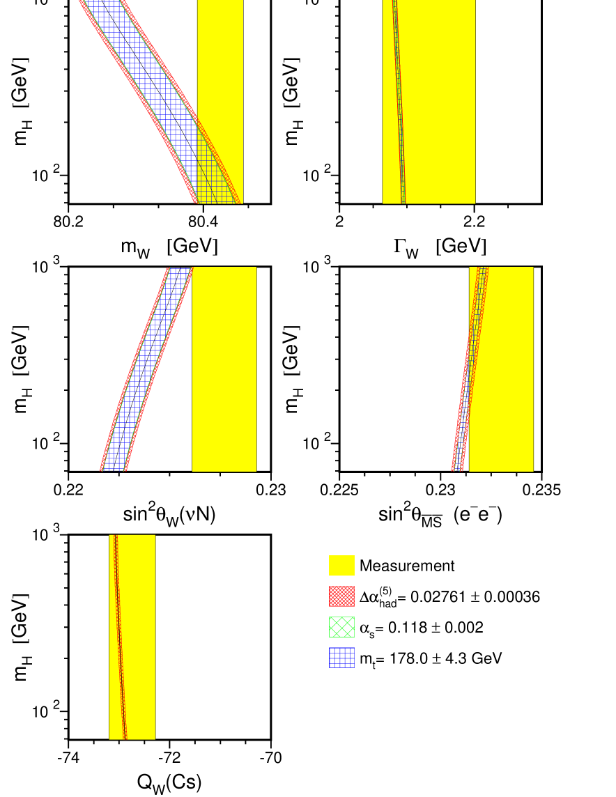
Figure 16.9: Comparison of $m_{\mathrm{W}}$ and $\Gamma_{\mathrm{W}}$ measured at LEP-2 and $\mathrm{p\overline{p}}$ colliders, of $\sin^{2}\theta_{\mathrm{W}}$ measured by NuTeV and of APV in caesium with the Standard Model prediction as a function of $m_{\mathrm{H}}$. The measurement with its error is shown as the vertical band. The width of the Standard Model band is due to the uncertainties in $\Delta\alpha^{(5)}_{\mathrm{had}}(m_{\mathrm{Z}}^{2})$, $\alpha_{\mathrm{S}}(m_{\mathrm{Z}}^{2})$ and $m_{\mathrm{t}}$. The total width of the band is the linear sum of these effects.

Chapter 17 Conclusions

The combination of the many precise electroweak results yields stringent constraints on the Standard Model. In addition, the results are sensitive to the Higgs mass. Most measurements agree well with the predictions. The spread in values of the various determinations of the effective electroweak mixing angle is somewhat larger than expected. Within the Standard Model analysis, this seems to be caused by the measurement of the forward-backward asymmetry in b-quark production, showing the largest pull of all Z-pole measurements w.r.t. the Standard Model expectation. The final result of the NuTeV collaboration on the electroweak mixing angle differs more, by close to three standard deviations from the Standard Model expectation calculated based on all other precision electroweak measurements.

The LEP and SLD experiments wish to stress that this report reflects a preliminary status of their results at the time of the 2004 summer conferences. A definitive statement on these results must wait for publication by each collaboration.

Prospects for the Future

Most of the measurements from data taken at or near the Z resonance, both at LEP as well as at SLC, that are presented in this report are either final or are being finalised. The main improvements will therefore take place in the high energy data, with more than 700 pb^-1 per experiment. The measurements of $m_{\mathrm{W}}$ are likely to reach a precision not too far from the uncertainty on the prediction obtained via the radiative corrections of the $\mathrm{Z}$ data, providing a further important test of the Standard Model. In the measurement of the triple and quartic electroweak gauge boson self couplings, the analysis of the complete LEP-II statistics, together with the increased sensitivity at higher beam energies, will lead to an improvement in the current precision.

Acknowledgements

We would like to thank the CERN accelerator divisions for the efficient operation of the LEP accelerator, the precise information on the absolute energy scale and their close cooperation with the four experiments. The SLD collaboration would like to thank the SLAC accelerator department for the efficient operation of the SLC accelerator. We would also like to thank members of the CDF, DØ and NuTeV collaborations for making results available to us in advance of the conferences and for useful discussions concerning their combination. Finally, the results of the section on Standard Model constraints would not be possible without the close collaboration of many theorists.

Appendix A The Measurements used in the Heavy-Flavour Averages

In the following 20 tables the results used in the combination are listed. In each case an indication of the dataset used and the type of analysis is given. The values of centre-of-mass energy are given where relevant. In each table, the result used as input to the average procedure is given followed by the statistical error, the correlated and uncorrelated systematic errors, the total systematic error, and any dependence on other electroweak parameters. In the case of the asymmetries, the measurement moved to a common energy (89.55 GeV, 91.26 GeV and 92.94 GeV, respectively, for peak$-$2, peak and peak+2 results) is quoted as corrected asymmetry.

Contributions to the correlated systematic error quoted here are from any sources of error shared with one or more other results from different experiments in the same table, and the uncorrelated errors from the remaining sources. In the case of ${\cal A}_{\mathrm{c}}$ and ${\cal A}_{\mathrm{b}}$ from SLD the quoted correlated systematic error has contributions from any source shared with one or more other measurements from LEP experiments. Constants such as $a(x)$ denote the dependence on the assumed value of $x^{\rm{used}}$, which is also given.

	ALEPH	DELPHI	L3	OPAL	SLD
	92-95	92-95	94-95	92-95	93-98
	multi	multi	multi	multi	multi
	[24]	[25]	[26]	[27]	[28]
Published $R_{\mathrm{b}}^{0}$	0.2159	0.21634	0.2174	0.2178	0.21603
Used $R_{\mathrm{b}}^{0}$	0.2158	0.21643	0.2166	0.2176	0.21580
Statistical	0.0009	0.00067	0.0013	0.0011	0.00094
Internal Systematic	0.0007	0.00038	0.0014	0.0009	0.00051
Common Systematic	0.0006	0.00039	0.0018	0.0008	0.00054
Other Param. Sys.	0.0001	0.00014	0.0010	0.0004	0.00016
Total Systematic	0.0009	0.00056	0.0025	0.0012	0.00076
Total Error	0.0013	0.00087	0.0028	0.0017	0.00121

Table A.1: The measurements of $R_{\mathrm{b}}^{0}$. All measurements use a lifetime tag enhanced by other features like invariant mass cuts or high $p_{T}$ leptons.

	ALEPH			DELPHI		OPAL		SLD
	91-95	91-95	92-95	92-95	92-95	91-94	90-95	93-97
	$D$-meson	$c$-count	lepton	$c$-count	$D$-meson	$c$-count	$D$-meson	$D$-meson
		(result)		(result)	(result)	(result)	(result)
	[29]	[33]	[29]	[31]	[30, 31]	[34]	[32]	[35]
Published $R_{\mathrm{c}}^{0}$	0.1689	0.1738	0.1675	0.1692	0.1610	0.167	0.180	0.17397
Used $R_{\mathrm{c}}^{0}$	0.1682	0.1735	0.1685	0.1693	0.1610	0.164	0.177	0.17440
Statistical	0.0082	0.0051	0.0062	0.0050	0.0104	0.012	0.010	0.00310
Internal Systematic	0.0077	0.0057	0.0042	0.0050	0.0064	0.013	0.010	0.00104
Common Systematic	0.0029	0.0094	0.0042	0.0077	0.0061	0.010	0.006	0.00163
Other Param. Sys.	0.0000	0.0000	0.0053	0.0000	0.0008	0.000	0.000	0.00042
Total Systematic	0.0082	0.0110	0.0080	0.0092	0.0089	0.016	0.012	0.00198
Total Error	0.0116	0.0122	0.0101	0.0105	0.0136	0.020	0.015	0.00368

Table A.2: The measurements of $R_{\mathrm{c}}^{0}$. “$c$-count” denotes the determination of $R_{\mathrm{c}}^{0}$ from the sum of production rates of weakly decaying charmed hadrons. “$D$-meson” denotes any single/double tag analysis using exclusive and/or inclusive $D$ meson reconstruction. The columns with the mention “(result)” are not directly used in the global average, only the corresponding measurements ($\mathrm{P(c\rightarrow D^{*+})}$ $\times$ $\mathrm{BR(D^{*+}\rightarrow\pi^{+}D^{0})}$, ${\rm{R_{c}f_{D^{+}}}}$, ${\rm{R_{c}f_{D_{s}}}}$, ${\rm{R_{c}f_{\Lambda_{c}}}}$, ${\rm{R_{c}f_{D^{0}}}}$and $\mathrm{R_{c}P(c\rightarrow D^{*+})\times BR(D^{*+}\rightarrow\pi^{+}D^{0})}$) are included.

	ALEPH				DELPHI			L3	OPAL
	91-95	91-95	91-95	91-95	91-95	92-95	92-00	90-95	91-00	90-00	90-95
	lepton	lepton	lepton	jet	lepton	$D$-meson	multi	lepton	jet	lepton	$D$-meson
	[39]	[39]	[39]	[43]	[40]	[48]	[44]	[41]	[46]	[42]	[49]
$\sqrt{s}$ (GeV)	88.38	89.38	90.21	89.47	89.434	89.434	89.449	89.50	89.50	89.51	89.49
Published $A_{\mathrm{FB}}^{\mathrm{b\overline{b}}}(-2)$	-13.10	5.47	-0.42	4.36	6.6	5.67	6.371	6.11	5.82	4.70	-8.6
Used $A_{\mathrm{FB}}^{\mathrm{b\overline{b}}}(-2)$	5.21			4.60	6.4	4.81	6.638	6.29	5.99	5.24	-4.8
Statistical	1.78			1.19	2.2	7.31	1.432	2.93	1.53	1.77	10.4
Internal Systematic	0.08			0.04	0.2	0.68	0.205	0.31	0.09	0.11	2.0
Common Systematic	0.10			0.01	0.1	0.21	0.025	0.17	0.04	0.05	1.1
Other Param. Sys.	0.15			0.14	0.2	0.75	0.021	0.07	0.09	0.16	0.8
Total Systematic	0.19			0.15	0.3	1.04	0.208	0.36	0.14	0.20	2.4
Total Error	1.79			1.20	2.2	7.39	1.447	2.95	1.54	1.78	10.7

Table A.3: The measurements of $A_{\mathrm{FB}}^{\mathrm{b\overline{b}}}(-2)$. The ”Used” values are quoted at $\sqrt{s}=89.55\,{\mathrm{Ge\kern-1.00006ptV}}$. All numbers are given in %.

	ALEPH				DELPHI		OPAL
	91-95	91-95	91-95	91-95	91-95	92-95	90-00	90-95
	lepton	lepton	lepton	$D$-meson	lepton	$D$-meson	lepton	$D$-meson
	[39]	[39]	[39]	[47]	[40]	[48]	[42]	[49]
$\sqrt{s}$ (GeV)	88.38	89.38	90.21	89.37	89.434	89.434	89.51	89.49
Published $A_{\mathrm{FB}}^{\mathrm{c\overline{c}}}(-2)$	-12.4	-2.28	-0.34	-1.0	3.0	-4.96	-6.83	3.9
Used $A_{\mathrm{FB}}^{\mathrm{c\overline{c}}}(-2)$	-1.50			0.2	3.4	-4.35	-6.23	2.5
Statistical	2.44			4.3	3.4	3.55	2.48	4.9
Internal Systematic	0.17			0.9	0.3	0.34	0.89	0.8
Common Systematic	0.07			0.1	0.1	0.11	0.09	0.3
Other Param. Sys.	0.14			0.2	0.2	0.10	0.25	0.1
Total Systematic	0.23			0.9	0.4	0.37	0.93	0.8
Total Error	2.45			4.4	3.5	3.57	2.65	5.0

Table A.4: The measurements of $A_{\mathrm{FB}}^{\mathrm{c\overline{c}}}(-2)$. The ”Used” values are quoted at $\sqrt{s}=89.55\,{\mathrm{Ge\kern-1.00006ptV}}$. All numbers are given in %.

	ALEPH		DELPHI			L3		OPAL
	91-95	91-95	91-95	92-95	92-00	91-95	90-95	91-00	90-00	90-95
	lepton	jet	lepton	$D$-meson	multi	jet	lepton	jet	lepton	$D$-meson
	[39]	[43]	[40]	[48]	[44]	[45]	[41]	[46]	[42]	[49]
$\sqrt{s}$ (GeV)	91.21	91.23	91.26	91.235	91.231	91.24	91.26	91.26	91.25	91.24
Published $A_{\mathrm{FB}}^{\mathrm{b\overline{b}}}(\mathrm{pk})$	9.52	10.00	10.04	7.62	9.58	9.31	9.80	9.77	9.716	9.4
Used $A_{\mathrm{FB}}^{\mathrm{b\overline{b}}}(\mathrm{pk})$	9.98	10.03	10.15	7.86	9.67	9.28	9.66	9.71	9.767	9.7
Statistical	0.40	0.27	0.55	1.90	0.32	1.01	0.65	0.36	0.398	2.6
Internal Systematic	0.07	0.10	0.17	0.53	0.15	0.51	0.27	0.15	0.073	2.1
Common Systematic	0.10	0.02	0.16	0.57	0.04	0.21	0.16	0.08	0.133	0.3
Other Param. Sys.	0.12	0.05	0.10	0.18	0.03	0.07	0.12	0.05	0.098	0.2
Total Systematic	0.17	0.12	0.25	0.80	0.15	0.56	0.33	0.18	0.180	2.1
Total Error	0.44	0.29	0.60	2.06	0.35	1.15	0.73	0.40	0.437	3.4

Table A.5: The measurements of $A_{\mathrm{FB}}^{\mathrm{b\overline{b}}}(\mathrm{pk})$. The ”Used” values are quoted at $\sqrt{s}=91.26\,{\mathrm{Ge\kern-1.00006ptV}}$. All numbers are given in %.

	ALEPH		DELPHI		L3	OPAL
	91-95	91-95	91-95	92-95	90-95	90-00	90-95
	lepton	$D$-meson	lepton	$D$-meson	lepton	lepton	$D$-meson
	[39]	[47]	[40]	[48]	[41]	[42]	[49]
$\sqrt{s}$ (GeV)	91.21	91.22	91.26	91.235	91.24	91.25	91.24
Published $A_{\mathrm{FB}}^{\mathrm{c\overline{c}}}(\mathrm{pk})$	6.45	6.3	6.31	6.59	7.84	5.683	6.3
Used $A_{\mathrm{FB}}^{\mathrm{c\overline{c}}}(\mathrm{pk})$	6.62	6.3	6.24	6.49	8.18	5.699	6.5
Statistical	0.56	0.9	0.92	0.93	3.03	0.539	1.2
Internal Systematic	0.24	0.2	0.52	0.26	1.71	0.192	0.5
Common Systematic	0.22	0.2	0.26	0.07	0.58	0.221	0.3
Other Param. Sys.	0.20	0.0	0.21	0.03	0.73	0.202	0.0
Total Systematic	0.38	0.3	0.61	0.27	1.95	0.356	0.6
Total Error	0.68	0.9	1.10	0.97	3.60	0.645	1.3

Table A.6: The measurements of $A_{\mathrm{FB}}^{\mathrm{c\overline{c}}}(\mathrm{pk})$. The ”Used” values are quoted at $\sqrt{s}=91.26\,{\mathrm{Ge\kern-1.00006ptV}}$. All numbers are given in %.

	ALEPH				DELPHI			L3	OPAL
	91-95	91-95	91-95	91-95	91-95	92-95	92-00	90-95	91-00	90-00	90-95
	lepton	lepton	lepton	jet	lepton	$D$-meson	multi	lepton	jet	lepton	$D$-meson
	[39]	[39]	[39]	[43]	[40]	[48]	[44]	[41]	[46]	[42]	[49]
$\sqrt{s}$ (GeV)	92.05	92.94	93.90	92.95	92.990	92.990	92.990	93.10	92.91	92.95	92.95
Published $A_{\mathrm{FB}}^{\mathrm{b\overline{b}}}(+2)$	11.10	10.43	13.77	11.72	10.9	8.82	10.41	13.71	12.21	10.31	-2.1
Used $A_{\mathrm{FB}}^{\mathrm{b\overline{b}}}(+2)$	11.11			11.69	11.4	8.59	10.40	13.70	12.24	10.06	-0.2
Statistical	1.43			0.98	1.8	6.16	1.16	2.39	1.23	1.47	8.7
Internal Systematic	0.19			0.11	0.1	0.88	0.27	0.30	0.16	0.09	2.0
Common Systematic	0.16			0.02	0.1	0.48	0.03	0.19	0.12	0.17	1.2
Other Param. Sys.	0.19			0.12	0.2	0.54	0.04	0.14	0.10	0.17	0.7
Total Systematic	0.31			0.16	0.3	1.14	0.28	0.38	0.23	0.26	2.4
Total Error	1.46			0.99	1.8	6.27	1.19	2.42	1.25	1.50	9.0

Table A.7: The measurements of $A_{\mathrm{FB}}^{\mathrm{b\overline{b}}}(+2)$. The ”Used” values are quoted at $\sqrt{s}=92.94\,{\mathrm{Ge\kern-1.00006ptV}}$. All numbers are given in %.

	ALEPH				DELPHI		OPAL
	91-95	91-95	91-95	91-95	91-95	92-95	90-00	90-95
	lepton	lepton	lepton	$D$-meson	lepton	$D$-meson	lepton	$D$-meson
	[39]	[39]	[39]	[47]	[40]	[48]	[42]	[49]
$\sqrt{s}$ (GeV)	92.05	92.94	93.90	92.96	92.990	92.990	92.95	92.95
Published $A_{\mathrm{FB}}^{\mathrm{c\overline{c}}}(+2)$	10.58	11.93	12.09	11.0	10.8	11.80	14.59	15.8
Used $A_{\mathrm{FB}}^{\mathrm{c\overline{c}}}(+2)$	11.93			10.9	10.8	11.42	14.89	14.6
Statistical	1.98			3.3	2.8	3.09	2.02	4.0
Internal Systematic	0.35			0.7	0.4	0.55	0.50	0.7
Common Systematic	0.29			0.1	0.2	0.09	0.24	0.5
Other Param. Sys.	0.34			0.2	0.3	0.09	0.43	0.1
Total Systematic	0.57			0.7	0.5	0.56	0.71	0.9
Total Error	2.06			3.4	2.8	3.15	2.14	4.1

Table A.8: The measurements of $A_{\mathrm{FB}}^{\mathrm{c\overline{c}}}(+2)$. The ”Used” values are quoted at $\sqrt{s}=92.94\,{\mathrm{Ge\kern-1.00006ptV}}$. All numbers are given in %.

	SLD
	93-98	93-98	94-95	96-98
	lepton	jet	$K^{\pm}$	$K$+vertex
	[50]	[52]	[53]	[54]
$\sqrt{s}$ (GeV)	91.28	91.28	91.28	91.28
Published ${\cal A}_{\mathrm{b}}$	0.919	0.907	0.855	0.919
Used ${\cal A}_{\mathrm{b}}$	0.939	0.907	0.855	0.9174
Statistical	0.030	0.020	0.088	0.0184
Internal Systematic	0.018	0.023	0.102	0.0169
Common Systematic	0.009	0.003	0.007	0.0032
Other Param. Sys.	0.011	0.001	0.000	0.0024
Total Systematic	0.023	0.024	0.102	0.0173
Total Error	0.037	0.031	0.135	0.0253

Table A.9: The measurements of ${\cal A}_{\mathrm{b}}$.

	SLD
	93-98	93-98	96-98
	lepton	$D$-meson	$K$+vertex
	[50]	[51]	[54]
$\sqrt{s}$ (GeV)	91.28	91.28	91.28
Published ${\cal A}_{\mathrm{c}}$	0.583	0.688	0.673
Used ${\cal A}_{\mathrm{c}}$	0.587	0.689	0.674
Statistical	0.055	0.035	0.029
Internal Systematic	0.045	0.020	0.023
Common Systematic	0.022	0.004	0.002
Other Param. Sys.	0.017	0.001	0.002
Total Systematic	0.053	0.021	0.023
Total Error	0.076	0.041	0.037

Table A.10: The measurements of ${\cal A}_{\mathrm{c}}$.

	ALEPH	DELPHI	L3		OPAL
	91-95	94-95	94-95	92	92-95	92-95
	multi	multi	multi	multi	multi	multi
	[55]	[56]	[26]	[57]	[58]	[58]
Published $\mathrm{BR}(\rm b\rightarrow\ell^{-})$	10.70	10.70	10.16	10.68	10.78	10.96
Used $\mathrm{BR}(\rm b\rightarrow\ell^{-})$	10.74	10.70	10.26	10.82	10.86
Statistical	0.10	0.14	0.09	0.11	0.09
Internal Systematic	0.15	0.14	0.16	0.36	0.21
Common Systematic	0.23	0.43	0.31	0.22	0.19
Other Param. Sys.	0.03	0.07	0.03	0.09	0.02
Total Systematic	0.28	0.45	0.35	0.43	0.29
Total Error	0.29	0.48	0.36	0.45	0.30

Table A.11: The measurements of $\mathrm{BR}(\rm b\rightarrow\ell^{-})$. All numbers are given in %.

	ALEPH	DELPHI	OPAL
	91-95	94-95	92-95	92-95
	multi	multi	multi	multi
	[55]	[56]	[58]	[58]
Published $\mathrm{BR}(\mathrm{b\rightarrow c\rightarrow\ell^{+}})$	8.18	7.98	8.37	8.17
Used $\mathrm{BR}(\mathrm{b\rightarrow c\rightarrow\ell^{+}})$	8.11	7.98	8.42
Statistical	0.15	0.22	0.15
Internal Systematic	0.18	0.16	0.22
Common Systematic	0.15	0.22	0.32
Other Param. Sys.	0.05	0.04	0.04
Total Systematic	0.24	0.27	0.39
Total Error	0.29	0.35	0.42

Table A.12: The measurements of $\mathrm{BR}(\mathrm{b\rightarrow c\rightarrow\ell^{+}})$. All numbers are given in %.

	DELPHI	OPAL
	92-95	90-95
	$D$+lepton	$D$+lepton
	[30]	[59]
Published $\mathrm{BR}(\mathrm{c}\rightarrow\ell^{+})$	9.58	9.5
Used $\mathrm{BR}(\mathrm{c}\rightarrow\ell^{+})$	9.67	9.6
Statistical	0.42	0.6
Internal Systematic	0.24	0.5
Common Systematic	0.13	0.4
Other Param. Sys.	0.01	0.0
Total Systematic	0.27	0.7
Total Error	0.50	0.9

Table A.13: The measurements of $\mathrm{BR}(\mathrm{c}\rightarrow\ell^{+})$. All numbers are given in %.

	ALEPH	DELPHI	L3	OPAL
	91-95	94-95	90-95	90-00
	multi	multi	lepton	lepton
	[39]	[56]	[41]	[42]
Published $\overline{\chi}$	0.11956	0.127	0.1192	0.13121
Used $\overline{\chi}$	0.11989	0.127	0.1199	0.13184
Statistical	0.00491	0.013	0.0066	0.00463
Internal Systematic	0.00206	0.005	0.0023	0.00149
Common Systematic	0.00402	0.003	0.0026	0.00369
Other Param. Sys.	0.00119	0.001	0.0016	0.00163
Total Systematic	0.00467	0.006	0.0038	0.00430
Total Error	0.00677	0.014	0.0076	0.00632

Table A.14: The measurements of $\overline{\chi}$.

	DELPHI	OPAL
	92-95	90-95
	$D$-meson	$D$-meson
	[30]	[32]
Published $\mathrm{P(c\rightarrow D^{*+})}$ $\times$ $\mathrm{BR(D^{*+}\rightarrow\pi^{+}D^{0})}$	0.174	0.15163
Used $\mathrm{P(c\rightarrow D^{*+})}$ $\times$ $\mathrm{BR(D^{*+}\rightarrow\pi^{+}D^{0})}$	0.174	0.15461
Statistical	0.010	0.00384
Internal Systematic	0.004	0.00451
Common Systematic	0.001	0.00499
Other Param. Sys.	0.000	0.00207
Total Systematic	0.004	0.00704
Total Error	0.011	0.00801

Table A.15: The measurements of $\mathrm{P(c\rightarrow D^{*+})}$ $\times$ $\mathrm{BR(D^{*+}\rightarrow\pi^{+}D^{0})}$.

	ALEPH	DELPHI	OPAL
	91-95	92-95	91-94
	$c$-count	$c$-count	$c$-count
	[33]	[31]	[34]
Published ${\rm{R_{c}f_{D^{+}}}}$	0.0409	0.03840	0.0393
Used ${\rm{R_{c}f_{D^{+}}}}$	0.0402	0.03860	0.0386
Statistical	0.0014	0.00135	0.0056
Internal Systematic	0.0012	0.00122	0.0026
Common Systematic	0.0029	0.00252	0.0028
Other Param. Sys.	0.0012	0.00080	0.0015
Total Systematic	0.0033	0.00291	0.0041
Total Error	0.0036	0.00321	0.0069

Table A.16: The measurements of ${\rm{R_{c}f_{D^{+}}}}$.

	ALEPH	DELPHI	OPAL
	91-95	92-95	91-94
	$c$-count	$c$-count	$c$-count
	[33]	[31]	[34]
Published ${\rm{R_{c}f_{D_{s}}}}$	0.0199	0.02129	0.0161
Used ${\rm{R_{c}f_{D_{s}}}}$	0.0206	0.02134	0.0158
Statistical	0.0036	0.00183	0.0048
Internal Systematic	0.0011	0.00089	0.0007
Common Systematic	0.0047	0.00480	0.0037
Other Param. Sys.	0.0003	0.00038	0.0006
Total Systematic	0.0048	0.00489	0.0038
Total Error	0.0060	0.00522	0.0061

Table A.17: The measurements of ${\rm{R_{c}f_{D_{s}}}}$.

	ALEPH	DELPHI	OPAL
	91-95	92-95	91-94
	$c$-count	$c$-count	$c$-count
	[33]	[31]	[34]
Published ${\rm{R_{c}f_{\Lambda_{c}}}}$	0.0169	0.01695	0.0107
Used ${\rm{R_{c}f_{\Lambda_{c}}}}$	0.0155	0.01702	0.0089
Statistical	0.0017	0.00396	0.0065
Internal Systematic	0.0005	0.00143	0.0008
Common Systematic	0.0038	0.00401	0.0028
Other Param. Sys.	0.0004	0.00039	0.0005
Total Systematic	0.0039	0.00428	0.0030
Total Error	0.0042	0.00583	0.0072

Table A.18: The measurements of ${\rm{R_{c}f_{\Lambda_{c}}}}$.

	ALEPH	DELPHI	OPAL
	91-95	92-95	91-94
	$c$-count	$c$-count	$c$-count
	[33]	[31]	[34]
Published ${\rm{R_{c}f_{D^{0}}}}$	0.0961	0.09274	0.1013
Used ${\rm{R_{c}f_{D^{0}}}}$	0.0966	0.09295	0.1027
Statistical	0.0031	0.00268	0.0080
Internal Systematic	0.0036	0.00264	0.0033
Common Systematic	0.0042	0.00239	0.0038
Other Param. Sys.	0.0018	0.00187	0.0016
Total Systematic	0.0058	0.00402	0.0053
Total Error	0.0066	0.00483	0.0095

Table A.19: The measurements of ${\rm{R_{c}f_{D^{0}}}}$.

	DELPHI	OPAL
	92-95	90-95
	$D$-meson	$D$-meson
	[31]	[32]
Published $\mathrm{R_{c}P(c\rightarrow D^{*+})\times BR(D^{*+}\rightarrow\pi^{+}D^{0})}$	0.02829	0.027180
Used $\mathrm{R_{c}P(c\rightarrow D^{*+})\times BR(D^{*+}\rightarrow\pi^{+}D^{0})}$	0.02837	0.027096
Statistical	0.00072	0.000472
Internal Systematic	0.00082	0.000838
Common Systematic	0.00060	0.001022
Other Param. Sys.	0.00087	0.000126
Total Systematic	0.00133	0.001328
Total Error	0.00151	0.001409

Table A.20: The measurements of $\mathrm{R_{c}P(c\rightarrow D^{*+})\times BR(D^{*+}\rightarrow\pi^{+}D^{0})}$.

Appendix B Heavy-Flavour Fit including Off-Peak Asymmetries

The full 18 parameter fit to the LEP and SLD data gave the following results:

$$R_{\mathrm{b}}^{0} = 0.21629\pm 0.00066$$

$$R_{\mathrm{c}}^{0} = 0.1723\pm 0.0031$$

$$A_{\mathrm{FB}}^{\mathrm{b\overline{b}}}(-2) = 0.0560\pm 0.0066$$

$$A_{\mathrm{FB}}^{\mathrm{c\overline{c}}}(-2) = -0.018\pm 0.013$$

$$A_{\mathrm{FB}}^{\mathrm{b\overline{b}}}(\mathrm{pk}) = 0.0982\pm 0.0017$$

$$A_{\mathrm{FB}}^{\mathrm{c\overline{c}}}(\mathrm{pk}) = 0.0635\pm 0.0036$$

$$A_{\mathrm{FB}}^{\mathrm{b\overline{b}}}(+2) = 0.1125\pm 0.0056$$

$$A_{\mathrm{FB}}^{\mathrm{c\overline{c}}}(+2) = 0.125\pm 0.011$$

$${\cal A}_{\mathrm{b}} = 0.924\pm 0.020$$

$${\cal A}_{\mathrm{c}} = 0.669\pm 0.027$$

$$\mathrm{BR}(\rm b\rightarrow\ell^{-}) = 0.1070\pm 0.0022$$

$$\mathrm{BR}(\mathrm{b\rightarrow c\rightarrow\ell^{+}}) = 0.0802\pm 0.0018$$

$$\mathrm{BR}(\mathrm{c}\rightarrow\ell^{+}) = 0.0971\pm 0.0031$$

$$\overline{\chi} = 0.1250\pm 0.0039$$

$$f({\rm D}^{+}) = 0.235\pm 0.016$$

$$f({\rm{D_{s}}}) = 0.125\pm 0.026$$

$$f({\mathrm{c_{baryon}}}) = 0.093\pm 0.022$$

$$\mathrm{P(c\rightarrow D^{*+})}\times\mathrm{BR(D^{*+}\rightarrow\pi^{+}D^{0})} = 0.1621\pm 0.0048\,$$

with a $\chi^{2}/$d.o.f. of $48/(105-18)$. The corresponding correlation matrix is given in Table B.1. The energy for the peak$-$2, peak and peak+2 results are respectively 89.55 GeV, 91.26 GeV and 92.94 GeV. Note that the asymmetry results shown here are not the pole asymmetries shown in Section 5.3.2. The non-electroweak parameters do not depend on the treatment of the asymmetries.

	$1)$	$2)$	$3)$	$4)$	$5)$	$6)$	$7)$	$8)$	$9)$	$10)$	$11)$	$12)$	$13)$	$14)$	$15)$	$16)$	$17)$	$18)$
	$R_{\mathrm{b}}$	$R_{\mathrm{c}}$	$A_{\mathrm{FB}}^{\mathrm{b\overline{b}}}$	$A_{\mathrm{FB}}^{\mathrm{c\overline{c}}}$	$A_{\mathrm{FB}}^{\mathrm{b\overline{b}}}$	$A_{\mathrm{FB}}^{\mathrm{c\overline{c}}}$	$A_{\mathrm{FB}}^{\mathrm{b\overline{b}}}$	$A_{\mathrm{FB}}^{\mathrm{c\overline{c}}}$	${\cal A}_{\mathrm{b}}$	${\cal A}_{\mathrm{c}}$	BR	BR	BR	$\overline{\chi}$	$f({\rm D}^{+})$	$f({\rm{D_{s}}})$	$f(c_{bar.})$	PcDst
			$(-2)$	$(-2)$	(pk)	(pk)	$(+2)$	$(+2)$			$(1)$	$(2)$	$(3)$
1)	$1.00$	$-0.18$	$-0.02$	$0.00$	$-0.10$	$0.07$	$-0.04$	$0.03$	$-0.08$	$0.04$	$-0.08$	$-0.03$	$0.00$	$0.00$	$-0.15$	$-0.03$	$0.11$	$0.13$
2)	$-0.18$	$1.00$	$0.01$	$0.01$	$0.03$	$-0.06$	$0.01$	$-0.04$	$0.04$	$-0.06$	$0.05$	$-0.01$	$-0.29$	$0.02$	$-0.12$	$0.17$	$0.16$	$-0.44$
3)	$-0.02$	$0.01$	$1.00$	$0.13$	$0.03$	$0.00$	$0.01$	$0.00$	$0.01$	$0.00$	$0.00$	$0.00$	$0.00$	$0.01$	$0.00$	$0.00$	$0.00$	$0.00$
4)	$0.00$	$0.01$	$0.13$	$1.00$	$0.01$	$0.02$	$0.01$	$0.01$	$0.00$	$0.00$	$0.01$	$-0.02$	$0.02$	$0.02$	$0.00$	$0.00$	$0.00$	$0.00$
5)	$-0.10$	$0.03$	$0.03$	$0.01$	$1.00$	$0.15$	$0.08$	$0.02$	$0.06$	$0.01$	$0.00$	$-0.05$	$0.00$	$0.11$	$0.01$	$0.00$	$-0.01$	$-0.02$
6)	$0.07$	$-0.06$	$0.00$	$0.02$	$0.15$	$1.00$	$0.02$	$0.15$	$-0.02$	$0.04$	$0.18$	$-0.23$	$-0.21$	$0.08$	$-0.03$	$-0.02$	$0.04$	$0.04$
7)	$-0.04$	$0.01$	$0.01$	$0.01$	$0.08$	$0.02$	$1.00$	$0.13$	$0.02$	$0.00$	$0.00$	$-0.03$	$0.00$	$0.03$	$0.01$	$0.00$	$0.00$	$-0.01$
8)	$0.03$	$-0.04$	$0.00$	$0.01$	$0.02$	$0.15$	$0.13$	$1.00$	$-0.01$	$0.02$	$0.07$	$-0.08$	$-0.14$	$0.02$	$-0.02$	$-0.02$	$0.02$	$0.02$
9)	$-0.08$	$0.04$	$0.01$	$0.00$	$0.06$	$-0.02$	$0.02$	$-0.01$	$1.00$	$0.11$	$-0.02$	$0.02$	$0.03$	$0.06$	$0.00$	$0.00$	$0.00$	$-0.02$
10)	$0.04$	$-0.06$	$0.00$	$0.00$	$0.01$	$0.04$	$0.00$	$0.02$	$0.11$	$1.00$	$0.02$	$-0.04$	$-0.02$	$0.00$	$0.00$	$0.00$	$0.00$	$0.02$
11)	$-0.08$	$0.05$	$0.00$	$0.01$	$0.00$	$0.18$	$0.00$	$0.07$	$-0.02$	$0.02$	$1.00$	$-0.24$	$0.00$	$0.29$	$0.04$	$0.01$	$-0.02$	$-0.01$
12)	$-0.03$	$-0.01$	$0.00$	$-0.02$	$-0.05$	$-0.23$	$-0.03$	$-0.08$	$0.02$	$-0.04$	$-0.24$	$1.00$	$0.10$	$-0.23$	$0.02$	$0.00$	$-0.01$	$0.01$
13)	$0.00$	$-0.29$	$0.00$	$0.02$	$0.00$	$-0.21$	$0.00$	$-0.14$	$0.03$	$-0.02$	$0.00$	$0.10$	$1.00$	$0.16$	$0.00$	$-0.02$	$-0.01$	$0.13$
14)	$0.00$	$0.02$	$0.01$	$0.02$	$0.11$	$0.08$	$0.03$	$0.02$	$0.06$	$0.00$	$0.29$	$-0.23$	$0.16$	$1.00$	$0.02$	$0.00$	$0.00$	$0.00$
15)	$-0.15$	$-0.12$	$0.00$	$0.00$	$0.01$	$-0.03$	$0.01$	$-0.02$	$0.00$	$0.00$	$0.04$	$0.02$	$0.00$	$0.02$	$1.00$	$-0.40$	$-0.25$	$0.09$
16)	$-0.03$	$0.17$	$0.00$	$0.00$	$0.00$	$-0.02$	$0.00$	$-0.02$	$0.00$	$0.00$	$0.01$	$0.00$	$-0.02$	$0.00$	$-0.40$	$1.00$	$-0.48$	$-0.08$
17)	$0.11$	$0.16$	$0.00$	$0.00$	$-0.01$	$0.04$	$0.00$	$0.02$	$0.00$	$0.00$	$-0.02$	$-0.01$	$-0.01$	$0.00$	$-0.25$	$-0.48$	$1.00$	$-0.13$
18)	$0.13$	$-0.44$	$0.00$	$0.00$	$-0.02$	$0.04$	$-0.01$	$0.02$	$-0.02$	$0.02$	$-0.01$	$0.01$	$0.13$	$0.00$	$0.09$	$-0.08$	$-0.13$	$1.00$

Table B.1: The correlation matrix for the set of the 18 heavy flavour parameters. BR(1), BR(2) and BR(3) denote $\mathrm{BR}(\rm b\rightarrow\ell^{-})$, $\mathrm{BR}(\mathrm{b\rightarrow c\rightarrow\ell^{+}})$ and $\mathrm{BR}(\mathrm{c}\rightarrow\ell^{+})$ respectively, PcDst denotes $\mathrm{P(c\rightarrow D^{*+})}\times\mathrm{BR(D^{*+}\rightarrow\pi^{+}D^{0})}$.

Appendix C Detailed inputs and results on W-boson and four-fermion averages

Tables C.1 - C.17 give the details of the inputs and of the results for the calculation of LEP averages of the four-fermion cross-section and the corresponding cross-section ratios For both inputs and results, whenever relevant, the breakdown of the errors into their various components is given in the table.

For each measurement, the Collaborations have privately provided unpublished information which is necessary for the combination of LEP results, such as the expected statistical error or the split up of the systematic uncertainty into its correlated and uncorrelated components. Unless otherwise specified in the References, all other inputs are taken from published papers and public notes submitted to conferences.

$\sqrt{s}$			(LCEC)	(LUEU)	(LUEC)
(GeV)	$\sigma_{\mathrm{WW}}$	$\Delta\sigma_{\mathrm{WW}}^{\mathrm{stat}}$	$\Delta\sigma_{\mathrm{WW}}^{\mathrm{syst}}$	$\Delta\sigma_{\mathrm{WW}}^{\mathrm{syst}}$	$\Delta\sigma_{\mathrm{WW}}^{\mathrm{syst}}$	$\Delta\sigma_{\mathrm{WW}}^{\mathrm{syst}}$	$\Delta\sigma_{\mathrm{WW}}$
ALEPH [130]
182.7	15.90	$\pm$0.61	$\pm$0.08	$\pm$0.08	$\pm$0.08	$\pm$0.14	$\pm$0.63
188.6	15.76	$\pm$0.34	$\pm$0.07	$\pm$0.05	$\pm$0.09	$\pm$0.12	$\pm$0.36
191.6	17.10	$\pm$0.89	$\pm$0.07	$\pm$0.07	$\pm$0.09	$\pm$0.14	$\pm$0.90
195.5	16.61	$\pm$0.52	$\pm$0.07	$\pm$0.06	$\pm$0.09	$\pm$0.12	$\pm$0.54
199.5	16.90	$\pm$0.50	$\pm$0.07	$\pm$0.06	$\pm$0.09	$\pm$0.12	$\pm$0.52
201.6	16.65	$\pm$0.70	$\pm$0.07	$\pm$0.07	$\pm$0.09	$\pm$0.13	$\pm$0.71
204.9	16.79	$\pm$0.52	$\pm$0.07	$\pm$0.06	$\pm$0.09	$\pm$0.13	$\pm$0.54
206.6	17.36	$\pm$0.41	$\pm$0.07	$\pm$0.06	$\pm$0.09	$\pm$0.13	$\pm$0.43
DELPHI [131]
182.7	16.07	$\pm$0.68	$\pm$0.09	$\pm$0.09	$\pm$0.08	$\pm$0.15	$\pm$0.70
188.6	16.09	$\pm$0.39	$\pm$0.08	$\pm$0.09	$\pm$0.09	$\pm$0.15	$\pm$0.42
191.6	16.64	$\pm$0.99	$\pm$0.09	$\pm$0.10	$\pm$0.09	$\pm$0.16	$\pm$1.00
195.5	17.04	$\pm$0.58	$\pm$0.09	$\pm$0.10	$\pm$0.09	$\pm$0.16	$\pm$0.60
199.5	17.39	$\pm$0.55	$\pm$0.09	$\pm$0.10	$\pm$0.09	$\pm$0.16	$\pm$0.57
201.6	17.37	$\pm$0.80	$\pm$0.10	$\pm$0.10	$\pm$0.09	$\pm$0.17	$\pm$0.82
204.9	17.56	$\pm$0.57	$\pm$0.10	$\pm$0.10	$\pm$0.09	$\pm$0.17	$\pm$0.59
206.6	16.35	$\pm$0.44	$\pm$0.10	$\pm$0.10	$\pm$0.09	$\pm$0.17	$\pm$0.47
L3 [132]
182.7	16.53	$\pm$0.67	$\pm$0.19	$\pm$0.13	$\pm$0.12	$\pm$0.26	$\pm$0.72
188.6	16.17	$\pm$0.37	$\pm$0.11	$\pm$0.06	$\pm$0.11	$\pm$0.17	$\pm$0.41
191.6	16.11	$\pm$0.90	$\pm$0.11	$\pm$0.07	$\pm$0.11	$\pm$0.17	$\pm$0.92
195.5	16.22	$\pm$0.54	$\pm$0.11	$\pm$0.06	$\pm$0.10	$\pm$0.16	$\pm$0.57
199.5	16.49	$\pm$0.56	$\pm$0.11	$\pm$0.07	$\pm$0.11	$\pm$0.17	$\pm$0.58
201.6	16.01	$\pm$0.82	$\pm$0.11	$\pm$0.06	$\pm$0.12	$\pm$0.17	$\pm$0.84
204.9	17.00	$\pm$0.58	$\pm$0.12	$\pm$0.06	$\pm$0.11	$\pm$0.17	$\pm$0.60
206.6	17.33	$\pm$0.44	$\pm$0.12	$\pm$0.04	$\pm$0.11	$\pm$0.17	$\pm$0.47
OPAL [133, 134]
182.7	15.43	$\pm$0.61	$\pm$0.14	$\pm$0.00	$\pm$0.22	$\pm$0.26	$\pm$0.66
188.6	16.30	$\pm$0.35	$\pm$0.11	$\pm$0.12	$\pm$0.07	$\pm$0.18	$\pm$0.39
191.6	16.60	$\pm$0.90	$\pm$0.23	$\pm$0.32	$\pm$0.14	$\pm$0.42	$\pm$0.99
195.5	18.59	$\pm$0.61	$\pm$0.23	$\pm$0.34	$\pm$0.14	$\pm$0.43	$\pm$0.75
199.5	16.32	$\pm$0.55	$\pm$0.23	$\pm$0.26	$\pm$0.14	$\pm$0.37	$\pm$0.67
201.6	18.48	$\pm$0.82	$\pm$0.23	$\pm$0.33	$\pm$0.14	$\pm$0.42	$\pm$0.92
204.9	15.97	$\pm$0.52	$\pm$0.23	$\pm$0.26	$\pm$0.14	$\pm$0.37	$\pm$0.64
206.6	17.77	$\pm$0.42	$\pm$0.23	$\pm$0.28	$\pm$0.14	$\pm$0.38	$\pm$0.57
LEP Averages								$\chi^{2}/\textrm{d.o.f.}$
182.7	15.89	$\pm$0.32	$\pm$0.10	$\pm$0.05	$\pm$0.06	$\pm$0.13	$\pm$0.35	$\left\}\begin{array}[h]{rr}&\hbox{\multirowsetup 26.4/24}\\ &\\ &\\ &\\ &\\ &\\ &\\ &\\ \end{array}\right.$
188.6	16.03	$\pm$0.18	$\pm$0.08	$\pm$0.04	$\pm$0.05	$\pm$0.10	$\pm$0.21
191.6	16.56	$\pm$0.46	$\pm$0.10	$\pm$0.08	$\pm$0.05	$\pm$0.14	$\pm$0.48
195.5	16.90	$\pm$0.29	$\pm$0.09	$\pm$0.06	$\pm$0.05	$\pm$0.12	$\pm$0.31
199.5	16.75	$\pm$0.27	$\pm$0.10	$\pm$0.06	$\pm$0.05	$\pm$0.13	$\pm$0.30
201.6	17.00	$\pm$0.39	$\pm$0.10	$\pm$0.07	$\pm$0.05	$\pm$0.13	$\pm$0.41
204.9	16.78	$\pm$0.28	$\pm$0.10	$\pm$0.07	$\pm$0.05	$\pm$0.13	$\pm$0.31
206.6	17.13	$\pm$0.22	$\pm$0.10	$\pm$0.06	$\pm$0.05	$\pm$0.13	$\pm$0.25

Table C.1: W-pair production cross-section (in pb) for different centre–of–mass energies. The first column contains the centre–of–mass energy and the second the measurements. Observed statistical uncertainties are used in the fit and are listed in the third column; when asymmetric errors are quoted by the Collaborations, the positive error is listed in the table and used in the fit. The fourth, fifth and sixth columns contain the components of the systematic errors, as subdivided by the Collaborations into LEP-correlated energy-correlated (LCEC), LEP-uncorrelated energy-uncorrelated (LUEU), LEP-uncorrelated energy-correlated (LUEC). The total systematic error is given in the seventh column, the total error in the eighth. For the LEP averages, the $\chi^{2}$ of the fit is also given in the ninth column.

$\sqrt{s}$(GeV)	182.7	188.6	191.6	195.5	199.5	201.6	204.9	206.6
182.7	1.000	0.160	0.090	0.128	0.137	0.100	0.141	0.165
188.6	0.160	1.000	0.116	0.168	0.179	0.131	0.182	0.216
191.6	0.090	0.116	1.000	0.092	0.099	0.072	0.101	0.119
195.5	0.128	0.168	0.092	1.000	0.142	0.104	0.145	0.171
199.5	0.137	0.179	0.099	0.142	1.000	0.111	0.154	0.182
201.6	0.100	0.131	0.072	0.104	0.111	1.000	0.113	0.133
204.9	0.141	0.182	0.101	0.145	0.154	0.113	1.000	0.186
206.6	0.165	0.216	0.119	0.171	0.182	0.133	0.186	1.000

Table C.2: Correlation matrix for the LEP combined W-pair cross-sections listed at the bottom of Table C.1. Correlations are all positive and range from 9% to 22%.

$\sqrt{s}$	WW cross-section (pb)
(GeV)	$\sigma_{\mathrm{WW}}^{\footnotesize\mbox{YFSWW}}$	$\sigma_{\mathrm{WW}}^{\footnotesize\mbox{RACOONWW}}$
182.7	$15.361\pm 0.005$	$15.368\pm 0.008$
188.6	$16.266\pm 0.005$	$16.249\pm 0.011$
191.6	$16.568\pm 0.006$	$16.519\pm 0.009$
195.5	$16.841\pm 0.006$	$16.801\pm 0.009$
199.5	$17.017\pm 0.007$	$16.979\pm 0.009$
201.6	$17.076\pm 0.006$	$17.032\pm 0.009$
204.9	$17.128\pm 0.006$	$17.079\pm 0.009$
206.6	$17.145\pm 0.006$	$17.087\pm 0.009$

Table C.3: W-pair cross-section predictions (in pb) for different centre–of–mass energies, according to YFSWW [139] and RACOONWW [140], for $m_{\mathrm{W}}=80.35$ GeV. The errors listed in the table are only the statistical errors from the numerical integration of the cross-section.

$\sqrt{s}$			(LCEU)	(LCEC)	(LUEU)	(LUEC)
(GeV)	${\cal{R}}_{\mathrm{WW}}$	$\Delta{\cal{R}}_{\mathrm{WW}}^{\mathrm{stat}}$	$\Delta{\cal{R}}_{\mathrm{WW}}^{\mathrm{syst}}$	$\Delta{\cal{R}}_{\mathrm{WW}}^{\mathrm{syst}}$	$\Delta{\cal{R}}_{\mathrm{WW}}^{\mathrm{syst}}$	$\Delta{\cal{R}}_{\mathrm{WW}}^{\mathrm{syst}}$	$\Delta{\cal{R}}_{\mathrm{WW}}$	$\chi^{2}/\textrm{d.o.f.}$
YFSWW [139]
182.7	1.034	$\pm$0.021	$\pm$0.000	$\pm$0.006	$\pm$0.003	$\pm$0.004	$\pm$0.023	$\left\}\begin{array}[h]{rr}&\hbox{\multirowsetup 26.4/24}\\ &\\ &\\ &\\ &\\ &\\ &\\ &\\ \end{array}\right.$
188.6	0.985	$\pm$0.011	$\pm$0.000	$\pm$0.005	$\pm$0.003	$\pm$0.003	$\pm$0.013
191.6	1.000	$\pm$0.028	$\pm$0.000	$\pm$0.006	$\pm$0.005	$\pm$0.003	$\pm$0.029
195.5	1.003	$\pm$0.017	$\pm$0.000	$\pm$0.006	$\pm$0.004	$\pm$0.003	$\pm$0.019
199.5	0.984	$\pm$0.016	$\pm$0.000	$\pm$0.006	$\pm$0.004	$\pm$0.003	$\pm$0.018
201.6	0.996	$\pm$0.023	$\pm$0.000	$\pm$0.006	$\pm$0.004	$\pm$0.003	$\pm$0.024
204.9	0.979	$\pm$0.016	$\pm$0.000	$\pm$0.006	$\pm$0.004	$\pm$0.003	$\pm$0.018
206.6	0.999	$\pm$0.013	$\pm$0.000	$\pm$0.006	$\pm$0.003	$\pm$0.003	$\pm$0.015
Average	0.993	$\pm$0.006	$\pm$0.000	$\pm$0.005	$\pm$0.001	$\pm$0.003	$\pm$0.009	32.3/31
RACOONWW [140]
182.7	1.034	$\pm$0.021	$\pm$0.001	$\pm$0.006	$\pm$0.003	$\pm$0.004	$\pm$0.023	$\left\}\begin{array}[h]{rr}&\hbox{\multirowsetup 26.4/24}\\ &\\ &\\ &\\ &\\ &\\ &\\ &\\ \end{array}\right.$
188.6	0.986	$\pm$0.011	$\pm$0.001	$\pm$0.005	$\pm$0.003	$\pm$0.003	$\pm$0.013
191.6	1.003	$\pm$0.028	$\pm$0.001	$\pm$0.006	$\pm$0.005	$\pm$0.003	$\pm$0.029
195.5	1.006	$\pm$0.017	$\pm$0.001	$\pm$0.006	$\pm$0.004	$\pm$0.003	$\pm$0.019
199.5	0.986	$\pm$0.016	$\pm$0.001	$\pm$0.006	$\pm$0.004	$\pm$0.003	$\pm$0.018
201.6	0.998	$\pm$0.023	$\pm$0.001	$\pm$0.006	$\pm$0.004	$\pm$0.003	$\pm$0.024
204.9	0.982	$\pm$0.016	$\pm$0.001	$\pm$0.006	$\pm$0.004	$\pm$0.003	$\pm$0.018
206.6	1.003	$\pm$0.013	$\pm$0.001	$\pm$0.006	$\pm$0.003	$\pm$0.003	$\pm$0.015
Average	0.995	$\pm$0.006	$\pm$0.000	$\pm$0.006	$\pm$0.001	$\pm$0.003	$\pm$0.009	32.0/31

Table C.4: Ratios of LEP combined W-pair cross-section measurements to the expectations of the considered theoretical models, for different centre–of–mass energies and for all energies combined. The first column contains the centre–of–mass energy, the second the combined ratios, the third the statistical errors. The fourth, fifth, sixth and seventh columns contain the sources of systematic errors that are considered as LEP-correlated energy-uncorrelated (LCEU), LEP-correlated energy-correlated (LCEC), LEP-uncorrelated energy-uncorrelated (LUEU), LEP-uncorrelated energy-correlated (LUEC). The total error is given in the eighth column. The only LCEU systematic sources considered are the statistical errors on the cross-section theoretical predictions, while the LCEC, LUEU and LUEC sources are those coming from the corresponding errors on the cross-section measurements. For the LEP averages, the $\chi^{2}$ of the fit is also given in the ninth column.

Decay			(unc)	(cor)			3$\times$3 correlation
channel	$\mathcal{B}$	$\Delta\mbox{$\mathcal{B}$}^{\mathrm{stat}}$	$\Delta\mbox{$\mathcal{B}$}^{\mathrm{syst}}$	$\Delta\mbox{$\mathcal{B}$}^{\mathrm{syst}}$	$\Delta\mbox{$\mathcal{B}$}^{\mathrm{syst}}$	$\Delta\mbox{$\mathcal{B}$}$	for $\Delta\mbox{$\mathcal{B}$}$
ALEPH [130]
$\mathcal{B}(\mathrm{W}\rightarrow\mathrm{e\overline{\nu}_{e}})$	10.81	$\pm$0.27	$\pm$0.09	$\pm$0.04	$\pm$0.10	$\pm$0.29	$\Biggl{(}\negthickspace\negthickspace$ -1.000 -0.012 -0.321 -0.012 -1.000 -0.268 -0.321 -0.268 -1.000 $\negthickspace\negthickspace\Biggr{)}$
$\mathcal{B}(\mathrm{W}\rightarrow\mu\overline{\nu}_{\mu})$	10.91	$\pm$0.25	$\pm$0.07	$\pm$0.04	$\pm$0.08	$\pm$0.26
$\mathcal{B}(\mathrm{W}\rightarrow\tau\overline{\nu}_{\tau})$	11.15	$\pm$0.32	$\pm$0.19	$\pm$0.05	$\pm$0.20	$\pm$0.38
DELPHI [131]
$\mathcal{B}(\mathrm{W}\rightarrow\mathrm{e\overline{\nu}_{e}})$	10.55	$\pm$0.31	$\pm$0.13	$\pm$0.05	$\pm$0.14	$\pm$0.34	$\Biggl{(}\negthickspace\negthickspace$ -1.000 0.030 -0.340 0.030 -1.000 -0.170 -0.340 -0.170 -1.000 $\negthickspace\negthickspace\Biggr{)}$
$\mathcal{B}(\mathrm{W}\rightarrow\mu\overline{\nu}_{\mu})$	10.65	$\pm$0.26	$\pm$0.06	$\pm$0.05	$\pm$0.08	$\pm$0.27
$\mathcal{B}(\mathrm{W}\rightarrow\tau\overline{\nu}_{\tau})$	11.46	$\pm$0.39	$\pm$0.17	$\pm$0.09	$\pm$0.19	$\pm$0.43
L3 [132]
$\mathcal{B}(\mathrm{W}\rightarrow\mathrm{e\overline{\nu}_{e}})$	10.78	$\pm$0.29	$\pm$0.10	$\pm$0.08	$\pm$0.13	$\pm$0.32	$\Biggl{(}\negthickspace\negthickspace$ -1.000 -0.016 -0.279 -0.016 -1.000 -0.295 -0.279 -0.295 -1.000 $\negthickspace\negthickspace\Biggr{)}$
$\mathcal{B}(\mathrm{W}\rightarrow\mu\overline{\nu}_{\mu})$	10.03	$\pm$0.29	$\pm$0.10	$\pm$0.07	$\pm$0.12	$\pm$0.31
$\mathcal{B}(\mathrm{W}\rightarrow\tau\overline{\nu}_{\tau})$	11.89	$\pm$0.40	$\pm$0.17	$\pm$0.11	$\pm$0.20	$\pm$0.45
OPAL [133, 134]
$\mathcal{B}(\mathrm{W}\rightarrow\mathrm{e\overline{\nu}_{e}})$	10.40	$\pm$0.25	$\pm$0.24	$\pm$0.05	$\pm$0.25	$\pm$0.35	$\Biggl{(}\negthickspace\negthickspace$ -1.000 0.141 -0.179 0.141 -1.000 -0.174 -0.179 -0.174 -1.000 $\negthickspace\negthickspace\Biggr{)}$
$\mathcal{B}(\mathrm{W}\rightarrow\mu\overline{\nu}_{\mu})$	10.61	$\pm$0.25	$\pm$0.23	$\pm$0.06	$\pm$0.24	$\pm$0.35
$\mathcal{B}(\mathrm{W}\rightarrow\tau\overline{\nu}_{\tau})$	11.18	$\pm$0.31	$\pm$0.37	$\pm$0.05	$\pm$0.37	$\pm$0.48
LEP Average (without lepton universality assumption)
$\mathcal{B}(\mathrm{W}\rightarrow\mathrm{e\overline{\nu}_{e}})$	10.66	$\pm$0.14	$\pm$0.07	$\pm$0.05	$\pm$0.09	$\pm$0.17	$\Biggl{(}\negthickspace\negthickspace$ -1.000 -0.109 -0.191 -0.109 -1.000 -0.132 -0.191 -0.132 -1.000 $\negthickspace\negthickspace\Biggr{)}$
$\mathcal{B}(\mathrm{W}\rightarrow\mu\overline{\nu}_{\mu})$	10.60	$\pm$0.13	$\pm$0.05	$\pm$0.05	$\pm$0.08	$\pm$0.15
$\mathcal{B}(\mathrm{W}\rightarrow\tau\overline{\nu}_{\tau})$	11.41	$\pm$0.18	$\pm$0.11	$\pm$0.07	$\pm$0.13	$\pm$0.22
$\chi^{2}/\textrm{d.o.f.}$	15.3/9
LEP Average (with lepton universality assumption)
$\mathcal{B}(\mathrm{W}\rightarrow\ell\overline{\nu}_{\ell})$	10.84	$\pm$0.06	$\pm$0.04	$\pm$0.06	$\pm$0.07	$\pm$0.09
$\mathcal{B}(\mathrm{W}\rightarrow\mathrm{had.})$	67.49	$\pm$0.19	$\pm$0.12	$\pm$0.18	$\pm$0.21	$\pm$0.28
$\chi^{2}/\textrm{d.o.f.}$	15.0/11

Table C.5: W branching fraction measurements (in %). The first column contains the decay channel, the second the measurements, the third the statistical uncertainty. The fourth and fifth column list the uncorrelated and correlated components of the systematic errors, as provided by the Collaborations. The total systematic error is given in the sixth column and the total error in the seventh. Correlation matrices for the three leptonic branching fractions are given in the last column.

DELPHI [131]

$\sqrt{s}$ interval (GeV)	Luminosity (pb-1)	Lumi weighted $\sqrt{s}$ (GeV)
180-184	51.63	182.65

cos$\theta_{W-}$ bin $i$	1	2	3	4	5	6	7	8	9	10
$\sigma_{i}$ (pb)	0.715	0.795	1.175	1.365	1.350	1.745	1.995	2.150	4.750	6.040
$\delta\sigma_{i}$(stat) (pb)	0.320	0.315	0.380	0.400	0.400	0.450	0.485	0.510	0.775	0.895
$\delta\sigma_{i}$(stat,exp.) (pb)	0.320	0.315	0.350	0.370	0.405	0.450	0.505	0.580	0.695	0.850
$\delta\sigma_{i}$(syst,unc) (pb)	0.020	0.025	0.035	0.035	0.040	0.085	0.050	0.065	0.095	0.075
$\delta\sigma_{i}$(syst,cor) (pb)	0.045	0.025	0.020	0.015	0.015	0.025	0.015	0.015	0.030	0.035

$\sqrt{s}$ interval (GeV)	Luminosity (pb-1)	Lumi weighted $\sqrt{s}$ (GeV)
184-194	178.32	189.03

cos$\theta_{W-}$ bin $i$	1	2	3	4	5	6	7	8	9	10
$\sigma_{i}$ (pb)	0.865	0.760	0.990	0.930	1.330	1.460	1.675	2.630	4.635	5.4000
$\delta\sigma_{i}$(stat) (pb)	0.180	0.170	0.185	0.180	0.215	0.225	0.240	0.300	0.405	0.4550
$\delta\sigma_{i}$(stat,exp.) (pb)	0.165	0.170	0.180	0.200	0.215	0.240	0.270	0.320	0.385	0.4900
$\delta\sigma_{i}$(syst,unc) (pb)	0.020	0.020	0.035	0.035	0.040	0.085	0.050	0.060	0.100	0.0850
$\delta\sigma_{i}$(syst,cor) (pb)	0.040	0.020	0.020	0.015	0.015	0.020	0.015	0.015	0.025	0.0350

$\sqrt{s}$ interval (GeV)	Luminosity (pb-1)	Lumi weighted $\sqrt{s}$ (GeV)
194-204	193.52	198.46

cos$\theta_{W-}$ bin $i$	1	2	3	4	5	6	7	8	9	10
$\sigma_{i}$ (pb)	0.600	0.675	1.510	1.150	1.055	1.635	2.115	3.175	4.470	7.1400
$\delta\sigma_{i}$(stat) (pb)	0.155	0.160	0.215	0.190	0.185	0.225	0.255	0.320	0.385	0.5000
$\delta\sigma_{i}$(stat,exp.) (pb)	0.150	0.160	0.170	0.180	0.200	0.230	0.260	0.310	0.380	0.5050
$\delta\sigma_{i}$(syst,unc) (pb)	0.015	0.020	0.030	0.035	0.035	0.085	0.045	0.055	0.105	0.1000
$\delta\sigma_{i}$(syst,cor) (pb)	0.025	0.015	0.015	0.015	0.015	0.015	0.010	0.015	0.025	0.0300

$\sqrt{s}$ interval (GeV)	Luminosity (pb-1)	Lumi weighted $\sqrt{s}$ (GeV)
204-210	198.59	205.91

cos$\theta_{W-}$ bin $i$	1	2	3	4	5	6	7	8	9	10
$\sigma_{i}$ (pb)	0.275	0.590	0.575	0.930	1.000	1.190	2.120	2.655	4.585	7.2900
$\delta\sigma_{i}$(stat) (pb)	0.120	0.145	0.140	0.170	0.175	0.195	0.255	0.290	0.385	0.5050
$\delta\sigma_{i}$(stat,exp.) (pb)	0.145	0.150	0.160	0.175	0.195	0.220	0.250	0.300	0.380	0.5200
$\delta\sigma_{i}$(syst,unc) (pb)	0.015	0.020	0.025	0.035	0.035	0.085	0.045	0.055	0.110	0.1100
$\delta\sigma_{i}$(syst,cor) (pb)	0.020	0.015	0.010	0.010	0.015	0.010	0.010	0.010	0.020	0.0300

Table C.6: W^- differential angular cross-section in the 10 angular bins for the four chosen energy intervals for the DELPHI experiment. For each energy range, the measured integrated luminosity and the luminosity weighted centre-of-mass energy is reported. The results per angular bin in each of the energy interval are then presented: $\sigma_{i}$ indicates the average of d[$\sigma_{\mathrm{WW}}$(BR_eν+BR_μν)]/dcos$\theta_{\mathrm{W}^{-}}$ in the $i$-th bin of cos$\theta_{\mathrm{W}^{-}}$ with width 0.2. The values, in each bin, of the measured and expected statistical error and of the systematic errors, LEP uncorrelated and correlated, are reported as well. All values are expressed in pb

L3 [132]

$\sqrt{s}$ interval (GeV)	Luminosity (pb-1)	Lumi weighted $\sqrt{s}$ (GeV)
180-184	55.46	182.68

cos$\theta_{W-}$ bin $i$	1	2	3	4	5	6	7	8	9	10
$\sigma_{i}$ (pb)	0.691	0.646	0.508	0.919	1.477	2.587	3.541	3.167	3.879	4.467
$\delta\sigma_{i}$(stat) (pb)	0.270	0.265	0.243	0.322	0.407	0.539	0.640	0.619	0.708	0.801
$\delta\sigma_{i}$(stat,exp.) (pb)	0.269	0.290	0.329	0.364	0.404	0.453	0.508	0.591	0.704	0.877
$\delta\sigma_{i}$(syst,unc) (pb)	0.016	0.009	0.007	0.011	0.018	0.031	0.043	0.039	0.048	0.058
$\delta\sigma_{i}$(syst,cor) (pb)	0.002	0.002	0.002	0.003	0.005	0.009	0.012	0.011	0.013	0.015

$\sqrt{s}$ interval (GeV)	Luminosity (pb-1)	Lumi weighted $\sqrt{s}$ (GeV)
184-194	206.49	189.16

cos$\theta_{W-}$ bin $i$	1	2	3	4	5	6	7	8	9	10
$\sigma_{i}$ (pb)	0.759	0.902	1.125	1.320	1.472	1.544	2.085	2.870	4.144	6.022
$\delta\sigma_{i}$(stat) (pb)	0.128	0.151	0.173	0.190	0.209	0.213	0.254	0.303	0.370	0.459
$\delta\sigma_{i}$(stat,exp.) (pb)	0.115	0.137	0.160	0.180	0.205	0.223	0.262	0.304	0.367	0.461
$\delta\sigma_{i}$(syst,unc) (pb)	0.017	0.013	0.015	0.015	0.017	0.018	0.024	0.034	0.048	0.074
$\delta\sigma_{i}$(syst,cor) (pb)	0.003	0.003	0.004	0.005	0.005	0.005	0.007	0.010	0.014	0.021

$\sqrt{s}$ interval (GeV)	Luminosity (pb-1)	Lumi weighted $\sqrt{s}$ (GeV)
194-204	203.50	198.30

cos$\theta_{W-}$ bin $i$	1	2	3	4	5	6	7	8	9	10
$\sigma_{i}$ (pb)	0.652	0.709	0.880	0.859	1.140	1.295	2.114	2.334	3.395	5.773
$\delta\sigma_{i}$(stat) (pb)	0.105	0.123	0.146	0.155	0.179	0.192	0.255	0.264	0.333	0.442
$\delta\sigma_{i}$(stat,exp.) (pb)	0.092	0.117	0.140	0.164	0.184	0.209	0.245	0.288	0.354	0.459
$\delta\sigma_{i}$(syst,unc) (pb)	0.014	0.010	0.011	0.010	0.013	0.015	0.024	0.027	0.040	0.071
$\delta\sigma_{i}$(syst,cor) (pb)	0.002	0.002	0.003	0.003	0.004	0.004	0.007	0.008	0.012	0.020

$\sqrt{s}$ interval (GeV)	Luminosity (pb-1)	Lumi weighted $\sqrt{s}$ (GeV)
204-210	217.30	205.96

cos$\theta_{W-}$ bin $i$	1	2	3	4	5	6	7	8	9	10
$\sigma_{i}$ (pb)	0.678	0.578	0.768	1.052	1.620	1.734	1.873	2.903	4.638	7.886
$\delta\sigma_{i}$(stat) (pb)	0.111	0.114	0.140	0.168	0.212	0.226	0.238	0.302	0.394	0.534
$\delta\sigma_{i}$(stat,exp.) (pb)	0.089	0.117	0.141	0.164	0.186	0.216	0.251	0.303	0.387	0.528
$\delta\sigma_{i}$(syst,unc) (pb)	0.015	0.008	0.010	0.012	0.019	0.020	0.021	0.034	0.054	0.097
$\delta\sigma_{i}$(syst,cor) (pb)	0.002	0.002	0.003	0.004	0.006	0.006	0.006	0.010	0.016	0.027

Table C.7: W^- differential angular cross-section in the 10 angular bins for the four chosen energy intervals for the L3 experiment. For each energy range, the measured integrated luminosity and the luminosity weighted centre-of-mass energy is reported. The results per angular bin in each of the energy interval are then presented: $\sigma_{i}$ indicates the average of d[$\sigma_{\mathrm{WW}}$(BR_eν+BR_μν)]/dcos$\theta_{\mathrm{W}^{-}}$ in the $i$-th bin of cos$\theta_{\mathrm{W}^{-}}$ with width 0.2. The values, in each bin, of the measured and expected statistical error and of the systematic errors, LEP uncorrelated and correlated, are reported as well. All values are expressed in pb

$\sqrt{s}$			(LCEC)	(LUEU)	(LUEC)
(GeV)	$\sigma_{\mathrm{We\nu\ (tot)}}$	$\Delta\sigma_{\mathrm{We\nu\ (tot)}}^{\mathrm{stat}}$	$\Delta\sigma_{\mathrm{We\nu\ (tot)}}^{\mathrm{syst}}$	$\Delta\sigma_{\mathrm{We\nu\ (tot)}}^{\mathrm{syst}}$	$\Delta\sigma_{\mathrm{We\nu\ (tot)}}^{\mathrm{syst}}$	$\Delta\sigma_{\mathrm{We\nu\ (tot)}}$	$\Delta\sigma_{\mathrm{We\nu\ (tot)}}^{\mathrm{stat\,(exp)}}$
ALEPH [147]
182.7	0.60	${}^{+0.32}_{-0.26}$	$\pm$0.02	$\pm$0.01	$\pm$0.01	${}^{+0.32}_{-0.26}$	$\pm$0.29
188.6	0.55	${}^{+0.18}_{-0.16}$	$\pm$0.02	$\pm$0.01	$\pm$0.01	${}^{+0.18}_{-0.16}$	$\pm$0.18
191.6	0.89	${}^{+0.58}_{-0.44}$	$\pm$0.02	$\pm$0.01	$\pm$0.02	${}^{+0.58}_{-0.44}$	$\pm$0.48
195.5	0.87	${}^{+0.31}_{-0.27}$	$\pm$0.03	$\pm$0.01	$\pm$0.02	${}^{+0.31}_{-0.27}$	$\pm$0.28
199.5	1.31	${}^{+0.32}_{-0.29}$	$\pm$0.03	$\pm$0.01	$\pm$0.02	${}^{+0.32}_{-0.29}$	$\pm$0.26
201.6	0.80	${}^{+0.42}_{-0.35}$	$\pm$0.03	$\pm$0.01	$\pm$0.02	${}^{+0.42}_{-0.35}$	$\pm$0.38
204.9	0.65	${}^{+0.27}_{-0.23}$	$\pm$0.03	$\pm$0.02	$\pm$0.02	${}^{+0.27}_{-0.23}$	$\pm$0.27
206.6	0.81	${}^{+0.22}_{-0.20}$	$\pm$0.03	$\pm$0.02	$\pm$0.02	${}^{+0.22}_{-0.20}$	$\pm$0.22
DELPHI [315, 316]
188.6	0.70	${}^{+0.29}_{-0.25}$	$\pm$0.00	$\pm$0.07	$\pm$0.00	${}^{+0.30}_{-0.26}$	$\pm$0.26
191.6	0.12	${}^{+0.29}_{-0.12}$	$\pm$0.00	$\pm$0.07	$\pm$0.00	${}^{+0.29}_{-0.14}$	$\pm$0.63
195.5	0.90	${}^{+0.39}_{-0.34}$	$\pm$0.00	$\pm$0.07	$\pm$0.00	${}^{+0.41}_{-0.36}$	$\pm$0.35
199.5	0.45	${}^{+0.31}_{-0.19}$	$\pm$0.00	$\pm$0.07	$\pm$0.00	${}^{+0.33}_{-0.20}$	$\pm$0.28
201.6	1.09	${}^{+0.52}_{-0.43}$	$\pm$0.00	$\pm$0.07	$\pm$0.00	${}^{+0.52}_{-0.43}$	$\pm$0.44
204.9	0.56	${}^{+0.36}_{-0.30}$	$\pm$0.00	$\pm$0.06	$\pm$0.00	${}^{+0.36}_{-0.30}$	$\pm$0.35
206.6	0.58	${}^{+0.25}_{-0.22}$	$\pm$0.00	$\pm$0.06	$\pm$0.00	${}^{+0.26}_{-0.23}$	$\pm$0.28
L3 [148, 149]
182.7	0.80	${}^{+0.28}_{-0.25}$	$\pm$0.04	$\pm$0.04	$\pm$0.01	${}^{+0.28}_{-0.25}$	$\pm$0.26
188.6	0.69	${}^{+0.16}_{-0.14}$	$\pm$0.03	$\pm$0.03	$\pm$0.01	${}^{+0.16}_{-0.15}$	$\pm$0.15
191.6	1.11	${}^{+0.48}_{-0.41}$	$\pm$0.02	$\pm$0.04	$\pm$0.01	${}^{+0.48}_{-0.41}$	$\pm$0.46
195.5	0.97	${}^{+0.27}_{-0.25}$	$\pm$0.02	$\pm$0.02	$\pm$0.01	${}^{+0.27}_{-0.25}$	$\pm$0.25
199.5	0.88	${}^{+0.26}_{-0.24}$	$\pm$0.02	$\pm$0.03	$\pm$0.01	${}^{+0.26}_{-0.24}$	$\pm$0.25
201.6	1.50	${}^{+0.45}_{-0.40}$	$\pm$0.03	$\pm$0.04	$\pm$0.02	${}^{+0.45}_{-0.40}$	$\pm$0.38
204.9	0.78	${}^{+0.29}_{-0.25}$	$\pm$0.02	$\pm$0.03	$\pm$0.01	${}^{+0.29}_{-0.25}$	$\pm$0.29
206.6	1.08	${}^{+0.21}_{-0.20}$	$\pm$0.02	$\pm$0.03	$\pm$0.01	${}^{+0.21}_{-0.20}$	$\pm$0.23
OPAL [317]
188.6 GeV	0.67	${}^{+0.16}_{-0.14}$	$\pm$0.04	$\pm$0.04	$\pm$0.00	${}^{+0.17}_{-0.15}$	$\pm$0.16
LEP							$\chi^{2}/\textrm{d.o.f.}$
182.7	0.70	$\pm$0.19	$\pm$0.03	$\pm$0.02	$\pm$0.01	$\pm$0.20	$\left\}\begin{array}[h]{rr}&\hbox{\multirowsetup 11.1/16}\\ &\\ &\\ &\\ &\\ &\\ &\\ &\\ \end{array}\right.$
188.6	0.64	$\pm$0.09	$\pm$0.03	$\pm$0.02	$\pm$0.01	$\pm$0.09
191.6	0.81	$\pm$0.29	$\pm$0.03	$\pm$0.02	$\pm$0.01	$\pm$0.30
195.5	0.91	$\pm$0.16	$\pm$0.02	$\pm$0.02	$\pm$0.01	$\pm$0.17
199.5	0.90	$\pm$0.15	$\pm$0.02	$\pm$0.02	$\pm$0.01	$\pm$0.16
201.6	1.12	$\pm$0.23	$\pm$0.02	$\pm$0.02	$\pm$0.01	$\pm$0.23
204.9	0.67	$\pm$0.17	$\pm$0.02	$\pm$0.02	$\pm$0.01	$\pm$0.18
206.6	0.85	$\pm$0.14	$\pm$0.02	$\pm$0.02	$\pm$0.01	$\pm$0.14

Table C.8: Single-W total production cross-section (in pb) at different energies. The first column contains the LEP centre–of–mass energy, and the second the measurements. The third column reports the statistical error, whereas in the fourth to the sixth columns the different systematic uncertainties are listed. The seventh column contains the total error and the eight lists, for the four LEP measurements, the symmetrized expected statistical error, and for the LEP combined value, the $\chi^{2}$ of the fit.

$\sqrt{s}$			(LCEC)	(LUEU)	(LUEC)
(GeV)	$\sigma_{\mathrm{We\nu\ (had)}}$	$\Delta\sigma_{\mathrm{We\nu\ (had)}}^{\mathrm{stat}}$	$\Delta\sigma_{\mathrm{We\nu\ (had)}}^{\mathrm{syst}}$	$\Delta\sigma_{\mathrm{We\nu\ (had)}}^{\mathrm{syst}}$	$\Delta\sigma_{\mathrm{We\nu\ (had)}}^{\mathrm{syst}}$	$\Delta\sigma_{\mathrm{We\nu\ (had)}}$	$\Delta\sigma_{\mathrm{We\nu\ (had)}}^{\mathrm{stat\,(exp)}}$
ALEPH [147]
182.7	0.44	${}^{+0.29}_{-0.24}$	$\pm$0.01	$\pm$0.01	$\pm$0.01	${}^{+0.29}_{-0.24}$	$\pm$0.26
188.6	0.33	${}^{+0.16}_{-0.14}$	$\pm$0.02	$\pm$0.01	$\pm$0.01	${}^{+0.16}_{-0.15}$	$\pm$0.16
191.6	0.52	${}^{+0.52}_{-0.40}$	$\pm$0.02	$\pm$0.01	$\pm$0.01	${}^{+0.52}_{-0.40}$	$\pm$0.45
195.5	0.61	${}^{+0.28}_{-0.25}$	$\pm$0.02	$\pm$0.01	$\pm$0.01	${}^{+0.28}_{-0.25}$	$\pm$0.25
199.5	1.06	${}^{+0.30}_{-0.27}$	$\pm$0.02	$\pm$0.01	$\pm$0.01	${}^{+0.30}_{-0.27}$	$\pm$0.24
201.6	0.72	${}^{+0.39}_{-0.33}$	$\pm$0.02	$\pm$0.01	$\pm$0.02	${}^{+0.39}_{-0.33}$	$\pm$0.34
204.9	0.34	${}^{+0.24}_{-0.21}$	$\pm$0.02	$\pm$0.01	$\pm$0.02	${}^{+0.24}_{-0.21}$	$\pm$0.25
206.6	0.64	${}^{+0.21}_{-0.19}$	$\pm$0.02	$\pm$0.01	$\pm$0.02	${}^{+0.21}_{-0.19}$	$\pm$0.19
DELPHI [315, 316]
188.6	0.44	${}^{+0.27}_{-0.24}$	$\pm$0.00	$\pm$0.07	$\pm$0.00	${}^{+0.28}_{-0.25}$	$\pm$0.25
191.6	0.01	${}^{+0.18}_{-0.01}$	$\pm$0.00	$\pm$0.07	$\pm$0.00	${}^{+0.19}_{-0.07}$	$\pm$0.57
195.5	0.78	${}^{+0.37}_{-0.33}$	$\pm$0.00	$\pm$0.07	$\pm$0.00	${}^{+0.38}_{-0.34}$	$\pm$0.33
199.5	0.16	${}^{+0.28}_{-0.16}$	$\pm$0.00	$\pm$0.07	$\pm$0.00	${}^{+0.29}_{-0.17}$	$\pm$0.27
201.6	0.55	${}^{+0.46}_{-0.39}$	$\pm$0.00	$\pm$0.07	$\pm$0.00	${}^{+0.47}_{-0.40}$	$\pm$0.43
204.9	0.50	${}^{+0.34}_{-0.30}$	$\pm$0.00	$\pm$0.06	$\pm$0.00	${}^{+0.35}_{-0.31}$	$\pm$0.33
206.6	0.37	${}^{+0.23}_{-0.20}$	$\pm$0.00	$\pm$0.06	$\pm$0.00	${}^{+0.24}_{-0.21}$	$\pm$0.26
L3 [148, 149]
182.7	0.58	${}^{+0.23}_{-0.20}$	$\pm$0.03	$\pm$0.03	$\pm$0.00	${}^{+0.23}_{-0.20}$	$\pm$0.21
188.6	0.52	${}^{+0.14}_{-0.13}$	$\pm$0.02	$\pm$0.02	$\pm$0.00	${}^{+0.14}_{-0.13}$	$\pm$0.14
191.6	0.84	${}^{+0.44}_{-0.37}$	$\pm$0.03	$\pm$0.03	$\pm$0.00	${}^{+0.44}_{-0.37}$	$\pm$0.41
195.5	0.66	${}^{+0.24}_{-0.22}$	$\pm$0.02	$\pm$0.03	$\pm$0.00	${}^{+0.25}_{-0.23}$	$\pm$0.21
199.5	0.37	${}^{+0.22}_{-0.20}$	$\pm$0.01	$\pm$0.02	$\pm$0.00	${}^{+0.22}_{-0.20}$	$\pm$0.22
201.6	1.10	${}^{+0.40}_{-0.35}$	$\pm$0.05	$\pm$0.05	$\pm$0.00	${}^{+0.40}_{-0.35}$	$\pm$0.35
204.9	0.42	${}^{+0.25}_{-0.21}$	$\pm$0.02	$\pm$0.03	$\pm$0.00	${}^{+0.25}_{-0.21}$	$\pm$0.25
206.6	0.66	${}^{+0.19}_{-0.17}$	$\pm$0.02	$\pm$0.03	$\pm$0.00	${}^{+0.20}_{-0.18}$	$\pm$0.20
OPAL [317]
188.6	0.53	${}^{+0.13}_{-0.12}$	$\pm$0.04	$\pm$0.04	$\pm$0.00	${}^{+0.14}_{-0.13}$	$\pm$0.14
LEP							$\chi^{2}/\textrm{d.o.f.}$
182.7	0.52	$\pm$0.16	$\pm$0.02	$\pm$0.02	$\pm$0.00	$\pm$0.17	$\left\}\begin{array}[h]{rr}&\hbox{\multirowsetup 11.9/16}\\ &\\ &\\ &\\ &\\ &\\ &\\ &\\ \end{array}\right.$
188.6	0.46	$\pm$0.08	$\pm$0.02	$\pm$0.02	$\pm$0.00	$\pm$0.08
191.6	0.54	$\pm$0.27	$\pm$0.02	$\pm$0.02	$\pm$0.00	$\pm$0.27
195.5	0.66	$\pm$0.15	$\pm$0.02	$\pm$0.02	$\pm$0.00	$\pm$0.15
199.5	0.55	$\pm$0.14	$\pm$0.01	$\pm$0.02	$\pm$0.01	$\pm$0.14
201.6	0.81	$\pm$0.21	$\pm$0.02	$\pm$0.03	$\pm$0.01	$\pm$0.21
204.9	0.40	$\pm$0.16	$\pm$0.01	$\pm$0.02	$\pm$0.01	$\pm$0.16
206.6	0.58	$\pm$0.12	$\pm$0.02	$\pm$0.02	$\pm$0.01	$\pm$0.13

Table C.9: Single-W hadronic production cross-section (in pb) at different energies. The first column contains the LEP centre–of–mass energy, and the second the measurements. The third column reports the statistical error, whereas in the fourth to the sixth columns the different systematic uncertainties are listed. The seventh column contains the total error and the eight lists, for the four LEP measurements, the symmetrized expected statistical error, and for the LEP combined value, the $\chi^{2}$ of the fit.

$\sqrt{s}$	We$\nu\rightarrow$qqe$\nu$ cross-section (pb)			We$\nu$ total cross-section (pb)
(GeV)	$\sigma_{\mathrm{We\nu\ (had)}}^{\footnotesize\mbox{\tt grc4f}}$	$\sigma_{\mathrm{We\nu\ (had)}}^{\footnotesize\mbox{WPHACT}}$	$\sigma_{\mathrm{We\nu\ (had)}}^{\footnotesize\mbox{WTO}}$	$\sigma_{\mathrm{We\nu\ (tot)}}^{\footnotesize\mbox{\tt grc4f}}$	$\sigma_{\mathrm{We\nu\ (tot)}}^{\footnotesize\mbox{WPHACT}}$
182.7	0.4194[1]	0.4070[2]	0.40934[8]	0.6254[1]	0.6066[2]
188.6	0.4699[1]	0.4560[2]	0.45974[9]	0.6999[1]	0.6796[2]
191.6	0.4960[1]	0.4810[2]	0.4852[1]	0.7381[2]	0.7163[2]
195.5	0.5308[2]	0.5152[2]	0.5207[1]	0.7896[2]	0.7665[3]
199.5	0.5673[2]	0.5509[3]	0.5573[1]	0.8431[2]	0.8182[3]
201.6	0.5870[2]	0.5704[4]	0.5768[1]	0.8718[2]	0.8474[4]
204.9	0.6196[2]	0.6021[4]	0.6093[2]	0.9185[3]	0.8921[4]
206.6	0.6358[2]	0.6179[4]	0.6254[2]	0.9423[3]	0.9157[5]

Table C.10: Single-W hadronic and total cross-section predictions (in pb) interpolated at the data centre–of–mass energies, according to the grc4f [152], WPHACT [151] and WTO [150] predictions. The numbers in brackets are the errors on the last digit and are coming from the numerical integration of the cross-section only.

$\sqrt{s}$			(LCEU)	(LCEC)	(LUEU)	(LUEC)
(GeV)	${\cal{R}}_{\mathrm{We\nu}}$	$\Delta{\cal{R}}_{\mathrm{We\nu}}^{\mathrm{stat}}$	$\Delta{\cal{R}}_{\mathrm{We\nu}}^{\mathrm{syst}}$	$\Delta{\cal{R}}_{\mathrm{We\nu}}^{\mathrm{syst}}$	$\Delta{\cal{R}}_{\mathrm{We\nu}}^{\mathrm{syst}}$	$\Delta{\cal{R}}_{\mathrm{We\nu}}^{\mathrm{syst}}$	$\Delta{\cal{R}}_{\mathrm{We\nu}}$	$\chi^{2}/\textrm{d.o.f.}$
grc4f [152]
182.7	1.121	$\pm$0.307	$\pm$0.001	$\pm$0.043	$\pm$0.031	$\pm$0.010	$\pm$0.312	$\left\}\begin{array}[h]{rr}&\hbox{\multirowsetup 11.1/16}\\ &\\ &\\ &\\ &\\ &\\ &\\ &\\ \end{array}\right.$
188.6	0.913	$\pm$0.126	$\pm$0.001	$\pm$0.036	$\pm$0.023	$\pm$0.007	$\pm$0.133
191.6	1.099	$\pm$0.398	$\pm$0.001	$\pm$0.024	$\pm$0.025	$\pm$0.010	$\pm$0.400
195.5	1.156	$\pm$0.206	$\pm$0.001	$\pm$0.022	$\pm$0.032	$\pm$0.009	$\pm$0.209
199.5	1.071	$\pm$0.181	$\pm$0.001	$\pm$0.020	$\pm$0.024	$\pm$0.008	$\pm$0.185
201.6	1.286	$\pm$0.263	$\pm$0.001	$\pm$0.024	$\pm$0.027	$\pm$0.010	$\pm$0.265
204.9	0.726	$\pm$0.188	$\pm$0.001	$\pm$0.020	$\pm$0.021	$\pm$0.008	$\pm$0.191
206.6	0.901	$\pm$0.144	$\pm$0.001	$\pm$0.021	$\pm$0.021	$\pm$0.009	$\pm$0.147
Average	0.973	$\pm$0.067	$\pm$0.000	$\pm$0.026	$\pm$0.010	$\pm$0.008	$\pm$0.073	16.0/23
WPHACT [151]
182.7	1.156	$\pm$0.317	$\pm$0.001	$\pm$0.044	$\pm$0.032	$\pm$0.010	$\pm$0.322	$\left\}\begin{array}[h]{rr}&\hbox{\multirowsetup 11.1/16}\\ &\\ &\\ &\\ &\\ &\\ &\\ &\\ \end{array}\right.$
188.6	0.941	$\pm$0.129	$\pm$0.001	$\pm$0.037	$\pm$0.026	$\pm$0.007	$\pm$0.137
191.6	1.133	$\pm$0.410	$\pm$0.001	$\pm$0.025	$\pm$0.033	$\pm$0.010	$\pm$0.412
195.5	1.192	$\pm$0.213	$\pm$0.001	$\pm$0.022	$\pm$0.025	$\pm$0.009	$\pm$0.216
199.5	1.103	$\pm$0.187	$\pm$0.001	$\pm$0.021	$\pm$0.028	$\pm$0.008	$\pm$0.190
201.6	1.325	$\pm$0.271	$\pm$0.001	$\pm$0.025	$\pm$0.028	$\pm$0.010	$\pm$0.273
204.9	0.748	$\pm$0.194	$\pm$0.001	$\pm$0.020	$\pm$0.022	$\pm$0.008	$\pm$0.196
206.6	0.923	$\pm$0.148	$\pm$0.001	$\pm$0.022	$\pm$0.022	$\pm$0.009	$\pm$0.152
Average	1.002	$\pm$0.069	$\pm$0.000	$\pm$0.027	$\pm$0.011	$\pm$0.008	$\pm$0.075	16.0/23

Table C.11: Ratios of LEP combined total single-W cross-section measurements to the expectations, for different centre–of–mass energies and for all energies combined. The first column contains the centre–of–mass energy, the second the combined ratios, the third the statistical errors. The fourth, fifth, sixth and seventh columns contain the sources of systematic errors that are considered as LEP-correlated energy-uncorrelated (LCEU), LEP-correlated energy-correlated (LCEC), LEP-uncorrelated energy-uncorrelated (LUEU), LEP-uncorrelated energy-correlated (LUEC). The total error is given in the eighth column. The only LCEU systematic sources considered are the statistical errors on the cross-section theoretical predictions, while the LCEC, LUEU and LUEC sources are those coming from the corresponding errors on the cross-section measurements.

$\sqrt{s}$			(LCEC)	(LUEU)	(LUEC)
(GeV)	$\sigma_{\mathrm{ZZ}}$	$\Delta\sigma_{\mathrm{ZZ}}^{\mathrm{stat}}$	$\Delta\sigma_{\mathrm{ZZ}}^{\mathrm{syst}}$	$\Delta\sigma_{\mathrm{ZZ}}^{\mathrm{syst}}$	$\Delta\sigma_{\mathrm{ZZ}}^{\mathrm{syst}}$	$\Delta\sigma_{\mathrm{ZZ}}$	$\Delta\sigma_{\mathrm{ZZ}}^{\mathrm{stat\,(exp)}}$
ALEPH [158, 159]
182.7	0.11	${}^{+0.16}_{-0.11}$	$\pm$0.01	$\pm$0.03	$\pm$0.03	${}^{+0.16}_{-0.12}$	$\pm$0.14
188.6	0.67	${}^{+0.13}_{-0.12}$	$\pm$0.01	$\pm$0.03	$\pm$0.03	${}^{+0.14}_{-0.13}$	$\pm$0.13
191.6	0.53	${}^{+0.34}_{-0.27}$	$\pm$0.01	$\pm$0.01	$\pm$0.01	${}^{+0.34}_{-0.27}$	$\pm$0.33
195.5	0.69	${}^{+0.23}_{-0.20}$	$\pm$0.01	$\pm$0.02	$\pm$0.02	${}^{+0.23}_{-0.20}$	$\pm$0.23
199.5	0.70	${}^{+0.22}_{-0.20}$	$\pm$0.01	$\pm$0.02	$\pm$0.02	${}^{+0.22}_{-0.20}$	$\pm$0.23
201.6	0.70	${}^{+0.33}_{-0.28}$	$\pm$0.01	$\pm$0.01	$\pm$0.01	${}^{+0.33}_{-0.28}$	$\pm$0.35
204.9	1.21	${}^{+0.26}_{-0.23}$	$\pm$0.01	$\pm$0.02	$\pm$0.02	${}^{+0.26}_{-0.23}$	$\pm$0.27
206.6	1.01	${}^{+0.19}_{-0.17}$	$\pm$0.01	$\pm$0.01	$\pm$0.01	${}^{+0.19}_{-0.17}$	$\pm$0.18
DELPHI [155]
182.7	0.35	${}^{+0.20}_{-0.15}$	$\pm$0.01	$\pm$0.00	$\pm$0.02	${}^{+0.20}_{-0.15}$	$\pm$0.16
188.6	0.52	${}^{+0.12}_{-0.11}$	$\pm$0.01	$\pm$0.00	$\pm$0.02	${}^{+0.12}_{-0.11}$	$\pm$0.13
191.6	0.63	${}^{+0.36}_{-0.30}$	$\pm$0.01	$\pm$0.01	$\pm$0.02	${}^{+0.36}_{-0.30}$	$\pm$0.35
195.5	1.05	${}^{+0.25}_{-0.22}$	$\pm$0.01	$\pm$0.01	$\pm$0.02	${}^{+0.25}_{-0.22}$	$\pm$0.21
199.5	0.75	${}^{+0.20}_{-0.18}$	$\pm$0.01	$\pm$0.01	$\pm$0.01	${}^{+0.20}_{-0.18}$	$\pm$0.21
201.6	0.85	${}^{+0.33}_{-0.28}$	$\pm$0.01	$\pm$0.01	$\pm$0.01	${}^{+0.33}_{-0.28}$	$\pm$0.32
204.9	1.03	${}^{+0.23}_{-0.20}$	$\pm$0.02	$\pm$0.01	$\pm$0.01	${}^{+0.23}_{-0.20}$	$\pm$0.23
206.6	0.96	${}^{+0.16}_{-0.15}$	$\pm$0.02	$\pm$0.01	$\pm$0.01	${}^{+0.16}_{-0.15}$	$\pm$0.17
L3 [156]
182.7	0.31	$\pm$0.16	$\pm$0.05	$\pm$0.00	$\pm$0.01	$\pm$0.17	$\pm$0.16
188.6	0.73	$\pm$0.15	$\pm$0.02	$\pm$0.02	$\pm$0.02	$\pm$0.15	$\pm$0.15
191.6	0.29	$\pm$0.22	$\pm$0.01	$\pm$0.01	$\pm$0.02	$\pm$0.22	$\pm$0.34
195.5	1.18	$\pm$0.24	$\pm$0.04	$\pm$0.05	$\pm$0.06	$\pm$0.26	$\pm$0.22
199.5	1.25	$\pm$0.25	$\pm$0.04	$\pm$0.05	$\pm$0.07	$\pm$0.27	$\pm$0.24
201.6	0.95	$\pm$0.38	$\pm$0.03	$\pm$0.04	$\pm$0.05	$\pm$0.39	$\pm$0.35
204.9	0.77	${}^{+0.21}_{-0.19}$	$\pm$0.01	$\pm$0.01	$\pm$0.04	${}^{+0.21}_{-0.19}$	$\pm$0.22
206.6	1.09	${}^{+0.17}_{-0.16}$	$\pm$0.02	$\pm$0.02	$\pm$0.06	${}^{+0.18}_{-0.17}$	$\pm$0.17
OPAL [157]
182.7	0.12	${}^{+0.20}_{-0.18}$	$\pm$0.00	$\pm$0.03	$\pm$0.00	${}^{+0.20}_{-0.18}$	$\pm$0.19
188.6	0.80	${}^{+0.14}_{-0.13}$	$\pm$0.01	$\pm$0.05	$\pm$0.03	${}^{+0.15}_{-0.14}$	$\pm$0.14
191.6	1.29	${}^{+0.47}_{-0.40}$	$\pm$0.02	$\pm$0.09	$\pm$0.05	${}^{+0.48}_{-0.41}$	$\pm$0.36
195.5	1.13	${}^{+0.26}_{-0.24}$	$\pm$0.02	$\pm$0.06	$\pm$0.05	${}^{+0.27}_{-0.25}$	$\pm$0.25
199.5	1.05	${}^{+0.25}_{-0.22}$	$\pm$0.02	$\pm$0.05	$\pm$0.04	${}^{+0.26}_{-0.23}$	$\pm$0.25
201.6	0.79	${}^{+0.35}_{-0.29}$	$\pm$0.02	$\pm$0.05	$\pm$0.03	${}^{+0.36}_{-0.30}$	$\pm$0.37
204.9	1.07	${}^{+0.27}_{-0.24}$	$\pm$0.02	$\pm$0.06	$\pm$0.04	${}^{+0.28}_{-0.25}$	$\pm$0.26
206.6	0.97	${}^{+0.19}_{-0.18}$	$\pm$0.02	$\pm$0.05	$\pm$0.04	${}^{+0.20}_{-0.19}$	$\pm$0.20
LEP							$\chi^{2}/\textrm{d.o.f.}$
182.7	0.22	$\pm$0.08	$\pm$0.02	$\pm$0.01	$\pm$0.01	$\pm$0.08	$\left\}\begin{array}[h]{rr}&\hbox{\multirowsetup 16.1/24}\\ &\\ &\\ &\\ &\\ &\\ &\\ &\\ \end{array}\right.$
188.6	0.66	$\pm$0.07	$\pm$0.01	$\pm$0.01	$\pm$0.01	$\pm$0.07
191.6	0.65	$\pm$0.17	$\pm$0.01	$\pm$0.02	$\pm$0.01	$\pm$0.17
195.5	0.99	$\pm$0.11	$\pm$0.02	$\pm$0.02	$\pm$0.02	$\pm$0.12
199.5	0.90	$\pm$0.12	$\pm$0.02	$\pm$0.02	$\pm$0.02	$\pm$0.12
201.6	0.81	$\pm$0.17	$\pm$0.02	$\pm$0.02	$\pm$0.01	$\pm$0.17
204.9	0.98	$\pm$0.12	$\pm$0.01	$\pm$0.01	$\pm$0.02	$\pm$0.13
206.6	0.99	$\pm$0.09	$\pm$0.02	$\pm$0.01	$\pm$0.02	$\pm$0.09

Table C.12: Z-pair production cross-section (in pb) at different energies. The first column contains the LEP centre–of–mass energy, the second the measurements and the third the statistical uncertainty. The fourth, the fifth and the sixth columns list the different components of the systematic errors, as provided by the Collaborations. The total error is given in the seventh column, whereas the eighth column lists, for the four LEP measurements, the symmetrized expected statistical error, and for the LEP combined value, the $\chi^{2}$ of the fit.

$\sqrt{s}$	ZZ cross-section (pb)
(GeV)	$\sigma_{\mathrm{ZZ}}^{\footnotesize\mbox{YFSZZ}}$	$\sigma_{\mathrm{ZZ}}^{\footnotesize\mbox{ZZTO}}$
182.7	0.254[1]	0.25425[2]
188.6	0.655[2]	0.64823[1]
191.6	0.782[2]	0.77670[1]
195.5	0.897[3]	0.89622[1]
199.5	0.981[2]	0.97765[1]
201.6	1.015[1]	1.00937[1]
204.9	1.050[1]	1.04335[1]
206.6	1.066[1]	1.05535[1]

Table C.13: Z-pair cross-section predictions (in pb) interpolated at the data centre–of–mass energies,according to the YFSZZ [160] and ZZTO [161] predictions. The numbers in brackets are the errors on the last digit and are coming from the numerical integration of the cross-section only.

$\sqrt{s}$			(LCEU)	(LCEC)	(LUEU)	(LUEC)
(GeV)	${\cal{R}}_{\mathrm{ZZ}}$	$\Delta{\cal{R}}_{\mathrm{ZZ}}^{\mathrm{stat}}$	$\Delta{\cal{R}}_{\mathrm{ZZ}}^{\mathrm{syst}}$	$\Delta{\cal{R}}_{\mathrm{ZZ}}^{\mathrm{syst}}$	$\Delta{\cal{R}}_{\mathrm{ZZ}}^{\mathrm{syst}}$	$\Delta{\cal{R}}_{\mathrm{ZZ}}^{\mathrm{syst}}$	$\Delta{\cal{R}}_{\mathrm{ZZ}}$	$\chi^{2}/\textrm{d.o.f.}$
YFSZZ [160]
182.7	0.857	$\pm$0.307	$\pm$0.018	$\pm$0.068	$\pm$0.041	$\pm$0.040	$\pm$0.320	$\left\}\begin{array}[h]{rr}&\hbox{\multirowsetup 16.1/24}\\ &\\ &\\ &\\ &\\ &\\ &\\ &\\ \end{array}\right.$
188.6	1.007	$\pm$0.104	$\pm$0.020	$\pm$0.019	$\pm$0.022	$\pm$0.018	$\pm$0.111
191.6	0.826	$\pm$0.220	$\pm$0.017	$\pm$0.014	$\pm$0.025	$\pm$0.017	$\pm$0.224
195.5	1.100	$\pm$0.127	$\pm$0.022	$\pm$0.021	$\pm$0.019	$\pm$0.020	$\pm$0.133
199.5	0.912	$\pm$0.119	$\pm$0.019	$\pm$0.018	$\pm$0.016	$\pm$0.017	$\pm$0.124
201.6	0.795	$\pm$0.170	$\pm$0.016	$\pm$0.017	$\pm$0.015	$\pm$0.013	$\pm$0.173
204.9	0.931	$\pm$0.116	$\pm$0.019	$\pm$0.014	$\pm$0.013	$\pm$0.014	$\pm$0.120
206.6	0.928	$\pm$0.085	$\pm$0.019	$\pm$0.014	$\pm$0.010	$\pm$0.015	$\pm$0.090
Average	0.945	$\pm$0.045	$\pm$0.008	$\pm$0.017	$\pm$0.006	$\pm$0.016	$\pm$0.052	19.1/31
ZZTO [161]
182.7	0.857	$\pm$0.307	$\pm$0.018	$\pm$0.068	$\pm$0.041	$\pm$0.040	$\pm$0.320	$\left\}\begin{array}[h]{rr}&\hbox{\multirowsetup 16.1/24}\\ &\\ &\\ &\\ &\\ &\\ &\\ &\\ \end{array}\right.$
188.6	1.017	$\pm$0.105	$\pm$0.021	$\pm$0.019	$\pm$0.022	$\pm$0.019	$\pm$0.113
191.6	0.831	$\pm$0.222	$\pm$0.017	$\pm$0.014	$\pm$0.025	$\pm$0.017	$\pm$0.225
195.5	1.100	$\pm$0.127	$\pm$0.022	$\pm$0.021	$\pm$0.019	$\pm$0.020	$\pm$0.133
199.5	0.915	$\pm$0.120	$\pm$0.019	$\pm$0.018	$\pm$0.016	$\pm$0.017	$\pm$0.125
201.6	0.799	$\pm$0.171	$\pm$0.016	$\pm$0.017	$\pm$0.015	$\pm$0.013	$\pm$0.174
204.9	0.937	$\pm$0.117	$\pm$0.019	$\pm$0.014	$\pm$0.013	$\pm$0.014	$\pm$0.121
206.6	0.937	$\pm$0.085	$\pm$0.019	$\pm$0.014	$\pm$0.011	$\pm$0.015	$\pm$0.091
Average	0.952	$\pm$0.046	$\pm$0.008	$\pm$0.017	$\pm$0.006	$\pm$0.016	$\pm$0.052	19.1/31

Table C.14: Ratios of LEP combined Z-pair cross-section measurements to the expectations, for different centre–of–mass energies and for all energies combined. The first column contains the centre–of–mass energy, the second the combined ratios, the third the statistical errors. The fourth, fifth, sixth and seventh columns contain the sources of systematic errors that are considered as LEP-correlated energy-uncorrelated (LCEU), LEP-correlated energy-correlated (LCEC), LEP-uncorrelated energy-uncorrelated (LUEU), LEP-uncorrelated energy-correlated (LUEC). The total error is given in the eighth column. The only LCEU systematic sources considered are the statistical errors on the cross-section theoretical predictions, while the LCEC, LUEU and LUEC sources are those coming from the corresponding errors on the cross-section measurements. For the LEP averages, the $\chi^{2}$ of the fit is also given in the ninth column.

$\sqrt{s}$			(LCEC)	(LUEU)	(LUEC)
(GeV)	$\sigma_{\mathrm{Zee}}$	$\Delta\sigma_{\mathrm{Zee}}^{\mathrm{stat}}$	$\Delta\sigma_{\mathrm{Zee}}^{\mathrm{syst}}$	$\Delta\sigma_{\mathrm{Zee}}^{\mathrm{syst}}$	$\Delta\sigma_{\mathrm{Zee}}^{\mathrm{syst}}$	$\Delta\sigma_{\mathrm{Zee}}$	$\Delta\sigma_{\mathrm{Zee}}^{\mathrm{stat\,(exp)}}$
ALEPH [147]
182.7	0.27	${}^{+0.21}_{-0.16}$	$\pm$0.01	$\pm$0.02	$\pm$0.01	${}^{+0.21}_{-0.16}$	$\pm$0.20
188.6	0.42	${}^{+0.14}_{-0.12}$	$\pm$0.01	$\pm$0.03	$\pm$0.01	${}^{+0.14}_{-0.12}$	$\pm$0.12
191.6	0.61	${}^{+0.39}_{-0.29}$	$\pm$0.01	$\pm$0.03	$\pm$0.01	${}^{+0.39}_{-0.29}$	$\pm$0.29
195.5	0.72	${}^{+0.24}_{-0.20}$	$\pm$0.01	$\pm$0.03	$\pm$0.01	${}^{+0.24}_{-0.20}$	$\pm$0.18
199.5	0.60	${}^{+0.21}_{-0.18}$	$\pm$0.01	$\pm$0.03	$\pm$0.01	${}^{+0.21}_{-0.18}$	$\pm$0.17
201.6	0.89	${}^{+0.35}_{-0.28}$	$\pm$0.01	$\pm$0.03	$\pm$0.01	${}^{+0.35}_{-0.28}$	$\pm$0.24
204.9	0.42	${}^{+0.17}_{-0.14}$	$\pm$0.01	$\pm$0.03	$\pm$0.01	${}^{+0.17}_{-0.15}$	$\pm$0.17
206.6	0.70	${}^{+0.17}_{-0.15}$	$\pm$0.01	$\pm$0.03	$\pm$0.01	${}^{+0.17}_{-0.15}$	$\pm$0.14
DELPHI [163]
182.7	0.56	${}^{+0.27}_{-0.22}$	$\pm$0.01	$\pm$0.06	$\pm$0.02	${}^{+0.28}_{-0.23}$	$\pm$0.24
188.6	0.65	${}^{+0.15}_{-0.14}$	$\pm$0.01	$\pm$0.03	$\pm$0.03	${}^{+0.16}_{-0.15}$	$\pm$0.14
191.6	0.63	${}^{+0.40}_{-0.30}$	$\pm$0.01	$\pm$0.03	$\pm$0.03	${}^{+0.40}_{-0.30}$	$\pm$0.33
195.5	0.66	${}^{+0.22}_{-0.18}$	$\pm$0.01	$\pm$0.02	$\pm$0.03	${}^{+0.22}_{-0.19}$	$\pm$0.19
199.5	0.57	${}^{+0.20}_{-0.17}$	$\pm$0.01	$\pm$0.02	$\pm$0.02	${}^{+0.20}_{-0.17}$	$\pm$0.18
201.6	0.19	${}^{+0.21}_{-0.16}$	$\pm$0.01	$\pm$0.02	$\pm$0.01	${}^{+0.21}_{-0.16}$	$\pm$0.25
204.9	0.37	${}^{+0.18}_{-0.15}$	$\pm$0.01	$\pm$0.02	$\pm$0.02	${}^{+0.18}_{-0.15}$	$\pm$0.19
206.6	0.68	${}^{+0.16}_{-0.14}$	$\pm$0.01	$\pm$0.02	$\pm$0.03	${}^{+0.16}_{-0.14}$	$\pm$0.14
L3 [162]
182.7	0.51	${}^{+0.19}_{-0.16}$	$\pm$0.02	$\pm$0.01	$\pm$0.03	${}^{+0.19}_{-0.16}$	$\pm$0.16
188.6	0.55	${}^{+0.10}_{-0.09}$	$\pm$0.02	$\pm$0.01	$\pm$0.03	${}^{+0.11}_{-0.10}$	$\pm$0.09
191.6	0.60	${}^{+0.26}_{-0.21}$	$\pm$0.01	$\pm$0.01	$\pm$0.03	${}^{+0.26}_{-0.21}$	$\pm$0.21
195.5	0.40	${}^{+0.13}_{-0.11}$	$\pm$0.01	$\pm$0.01	$\pm$0.03	${}^{+0.13}_{-0.11}$	$\pm$0.13
199.5	0.33	${}^{+0.12}_{-0.10}$	$\pm$0.01	$\pm$0.01	$\pm$0.03	${}^{+0.13}_{-0.11}$	$\pm$0.14
201.6	0.81	${}^{+0.27}_{-0.23}$	$\pm$0.02	$\pm$0.02	$\pm$0.03	${}^{+0.27}_{-0.23}$	$\pm$0.19
204.9	0.56	${}^{+0.16}_{-0.14}$	$\pm$0.01	$\pm$0.01	$\pm$0.03	${}^{+0.16}_{-0.14}$	$\pm$0.14
206.6	0.59	${}^{+0.12}_{-0.10}$	$\pm$0.01	$\pm$0.01	$\pm$0.03	${}^{+0.12}_{-0.11}$	$\pm$0.11
LEP							$\chi^{2}/\textrm{d.o.f.}$
182.7	0.45	$\pm$0.11	$\pm$0.01	$\pm$0.02	$\pm$0.01	$\pm$0.11	$\left\}\begin{array}[h]{rr}&\hbox{\multirowsetup 12.4/16}\\ &\\ &\\ &\\ &\\ &\\ &\\ &\\ \end{array}\right.$
188.6	0.53	$\pm$0.07	$\pm$0.01	$\pm$0.01	$\pm$0.01	$\pm$0.07
191.6	0.61	$\pm$0.15	$\pm$0.01	$\pm$0.02	$\pm$0.01	$\pm$0.15
195.5	0.55	$\pm$0.09	$\pm$0.01	$\pm$0.01	$\pm$0.01	$\pm$0.10
199.5	0.47	$\pm$0.09	$\pm$0.01	$\pm$0.02	$\pm$0.01	$\pm$0.10
201.6	0.67	$\pm$0.13	$\pm$0.01	$\pm$0.01	$\pm$0.01	$\pm$0.13
204.9	0.47	$\pm$0.10	$\pm$0.01	$\pm$0.01	$\pm$0.01	$\pm$0.10
206.6	0.65	$\pm$0.07	$\pm$0.01	$\pm$0.01	$\pm$0.01	$\pm$0.08

Table C.15: Single-Z hadronic production cross-section (in pb) at different energies. The first column contains the LEP centre–of–mass energy, and the second the measurements. The third column reports the statistical error, whereas in the fourth to the sixth columns the different systematic uncertainties are listed. The seventh column contains the total error and the eight lists, for the four LEP measurements, the symmetrized expected statistical error, and for the LEP combined value, the $\chi^{2}$ of the fit.

$\sqrt{s}$	Zee cross-section (pb)
(GeV)	$\sigma_{\mathrm{Zee}}^{\footnotesize\mbox{WPHACT}}$	$\sigma_{\mathrm{Zee}}^{\footnotesize\mbox{\tt grc4f}}$
182.7	0.51275[4]	0.51573[4]
188.6	0.53686[4]	0.54095[5]
191.6	0.54883[4]	0.55314[5]
195.5	0.56399[5]	0.56891[4]
199.5	0.57935[5]	0.58439[4]
201.6	0.58708[4]	0.59243[4]
204.9	0.59905[4]	0.60487[4]
206.6	0.61752[4]	0.60819[4]

Table C.16: Zee cross-section predictions (in pb) interpolated at the data centre–of–mass energies,according to the WPHACT [151] and grc4f [152] predictions. The numbers in brackets are the errors on the last digit and are coming from the numerical integration of the cross-section only.

$\sqrt{s}$			(LCEU)	(LCEC)	(LUEU)	(LUEC)
(GeV)	${\cal{R}}_{\mathrm{Zee}}$	$\Delta{\cal{R}}_{\mathrm{Zee}}^{\mathrm{stat}}$	$\Delta{\cal{R}}_{\mathrm{Zee}}^{\mathrm{syst}}$	$\Delta{\cal{R}}_{\mathrm{Zee}}^{\mathrm{syst}}$	$\Delta{\cal{R}}_{\mathrm{Zee}}^{\mathrm{syst}}$	$\Delta{\cal{R}}_{\mathrm{Zee}}^{\mathrm{syst}}$	$\Delta{\cal{R}}_{\mathrm{Zee}}$	$\chi^{2}/\textrm{d.o.f.}$
grc4f [152]
182.7	0.870	$\pm$0.214	$\pm$0.000	$\pm$0.020	$\pm$0.035	$\pm$0.025	$\pm$0.219	$\left\}\begin{array}[h]{rr}&\hbox{\multirowsetup 12.4/16}\\ &\\ &\\ &\\ &\\ &\\ &\\ &\\ \end{array}\right.$
188.6	0.983	$\pm$0.120	$\pm$0.000	$\pm$0.022	$\pm$0.023	$\pm$0.024	$\pm$0.126
191.6	1.104	$\pm$0.272	$\pm$0.000	$\pm$0.019	$\pm$0.027	$\pm$0.025	$\pm$0.276
195.5	0.963	$\pm$0.163	$\pm$0.000	$\pm$0.016	$\pm$0.024	$\pm$0.025	$\pm$0.167
199.5	0.809	$\pm$0.160	$\pm$0.000	$\pm$0.018	$\pm$0.030	$\pm$0.023	$\pm$0.165
201.6	1.129	$\pm$0.219	$\pm$0.000	$\pm$0.023	$\pm$0.024	$\pm$0.021	$\pm$0.223
204.9	0.770	$\pm$0.157	$\pm$0.000	$\pm$0.019	$\pm$0.019	$\pm$0.021	$\pm$0.161
206.6	1.061	$\pm$0.119	$\pm$0.000	$\pm$0.018	$\pm$0.018	$\pm$0.024	$\pm$0.124
Average	0.955	$\pm$0.057	$\pm$0.000	$\pm$0.019	$\pm$0.009	$\pm$0.023	$\pm$0.065	17.0/23
WPHACT [151]
182.7	0.875	$\pm$0.215	$\pm$0.000	$\pm$0.020	$\pm$0.035	$\pm$0.025	$\pm$0.220	$\left\}\begin{array}[h]{rr}&\hbox{\multirowsetup 12.9/16}\\ &\\ &\\ &\\ &\\ &\\ &\\ &\\ \end{array}\right.$
188.6	0.990	$\pm$0.120	$\pm$0.000	$\pm$0.022	$\pm$0.023	$\pm$0.025	$\pm$0.127
191.6	1.112	$\pm$0.274	$\pm$0.000	$\pm$0.020	$\pm$0.027	$\pm$0.026	$\pm$0.278
195.5	0.971	$\pm$0.164	$\pm$0.000	$\pm$0.016	$\pm$0.025	$\pm$0.025	$\pm$0.169
199.5	0.816	$\pm$0.161	$\pm$0.000	$\pm$0.019	$\pm$0.030	$\pm$0.023	$\pm$0.167
201.6	1.139	$\pm$0.221	$\pm$0.000	$\pm$0.023	$\pm$0.024	$\pm$0.021	$\pm$0.224
204.9	0.777	$\pm$0.158	$\pm$0.000	$\pm$0.019	$\pm$0.019	$\pm$0.021	$\pm$0.162
206.6	1.067	$\pm$0.120	$\pm$0.000	$\pm$0.018	$\pm$0.018	$\pm$0.024	$\pm$0.125
Average	0.963	$\pm$0.057	$\pm$0.000	$\pm$0.020	$\pm$0.009	$\pm$0.024	$\pm$0.065	16.9/23

Table C.17: Ratios of LEP combined single-Z cross-section measurements to the expectations, for different centre–of–mass energies and for all energies combined. The first column contains the centre–of–mass energy, the second the combined ratios, the third the statistical errors. The fourth, fifth, sixth and seventh columns contain the sources of systematic errors that are considered as LEP-correlated energy-uncorrelated (LCEU), LEP-correlated energy-correlated (LCEC), LEP-uncorrelated energy-uncorrelated (LUEU), LEP-uncorrelated energy-correlated (LUEC). The total error is given in the eighth column. The only LCEU systematic sources considered are the statistical errors on the cross-section theoretical predictions, while the LCEC, LUEU and LUEC sources are those coming from the corresponding errors on the cross-section measurements. For the LEP averages, the $\chi^{2}$ of the fit is also given in the ninth column.

Appendix D Colour Reconnection Combination

D.1 Inputs

	Experiment
$R_{N}$	ALEPH	DELPHI	L3	OPAL
Data	$1.0951\pm 0.0135$	$0.8996\pm 0.0314$	$0.8436\pm 0.0217$	$1.2570\pm 0.0251$
SK-I (100%)	$1.0548\pm 0.0012$	$0.8463\pm 0.0036$	$0.7482\pm 0.0033$	$1.1386\pm 0.0027$
JETSET	$1.1365\pm 0.0013$	$0.9444\pm 0.0039$	$0.8622\pm 0.0037$	$1.2958\pm 0.0028$
AR-2	$1.1341\pm 0.0013$	$0.9552\pm 0.0041$	$0.8696\pm 0.0037$	$1.2887\pm 0.0028$
ARIADNE	$1.1461\pm 0.0013$	$0.9530\pm 0.0039$	$0.8754\pm 0.0037$	$1.3057\pm 0.0028$
HERWIG CR	$1.1416\pm 0.0013$	$0.9649\pm 0.0039$	$0.8805\pm 0.0037$	$1.3016\pm 0.0029$
HERWIG	$1.1548\pm 0.0013$	$0.9675\pm 0.0040$	$0.8822\pm 0.0038$	$1.3204\pm 0.0029$
Systematics
Intra-W BEC	$\pm 0.0020$	$\pm 0.0094$	$\pm 0.0017$	$\pm 0.0015$
$\mathrm{e}^{+}\mathrm{e}^{-}\rightarrow\mathrm{q\overline{q}}$ shape	$\pm 0.0012$	$\pm 0.0013$	$\pm 0.0086$	$\pm 0.0035$
$\pm 10$% $\sigma(\mathrm{e}^{+}\mathrm{e}^{-}\rightarrow\mathrm{q\overline{q}})$	$\pm 0.0036$	$\pm 0.0042$	$\pm 0.0071$	$\pm 0.0040$
$\pm 15$% $\sigma(\mathrm{ZZ}\rightarrow\mathrm{q\overline{q}}\mathrm{q\overline{q}})$	$\pm 0.0004$	$\pm 0.0001$	$\pm 0.0020$	$\pm 0.0013$
Detector effects	$0.0040$	$-$	$\pm 0.0016$	$\pm 0.0072$
$E_{\mathrm{cm}}$ dependence	$\pm 0.0062$	$\pm 0.0012$	$\pm 0.0020$	$\pm 0.0030$

Table D.1: Inputs provided by the experiments for the combination.

$k_{i}$	$P_{reco}$ (%)	ALEPH	DELPHI	L3	OPAL
0.10	07.2	$1.1357\pm 0.0057$	$0.9410\pm 0.0034$	$0.8613\pm 0.0037$	$1.2887\pm 0.0028$
0.15	10.2	$1.1341\pm 0.0057$	$0.9393\pm 0.0032$	0.8598 $\pm$ 0.0037	$1.2859\pm 0.0028$
0.20	13.4	$1.1336\pm 0.0057$	$0.9378\pm 0.0031$	0.8585 $\pm$ 0.0037	$1.2823\pm 0.0028$
0.25	16.1	$1.1336\pm 0.0057$	$0.9363\pm 0.0030$	0.8561 $\pm$ 0.0037	$1.2800\pm 0.0028$
0.35	21.4	$1.1303\pm 0.0057$	$0.9334\pm 0.0028$	0.8551 $\pm$ 0.0037	$1.2741\pm 0.0028$
0.45	25.9	$1.1269\pm 0.0057$	$0.9307\pm 0.0027$	0.8509 $\pm$ 0.0036	$1.2693\pm 0.0028$
0.60	32.1	$1.1216\pm 0.0057$	$0.9271\pm 0.0025$	0.8482 $\pm$ 0.0036	$1.2639\pm 0.0028$
0.80	39.1	$1.1166\pm 0.0056$	$0.9227\pm 0.0024$	0.8414 $\pm$ 0.0037	$1.2576\pm 0.0028$
1.00	44.9	$1.1109\pm 0.0056$	$0.9189\pm 0.0024$	0.8381 $\pm$ 0.0036	$1.2499\pm 0.0028$
1.50	55.9	$1.1048\pm 0.0056$	$0.9110\pm 0.0025$	0.8318 $\pm$ 0.0036	$1.2368\pm 0.0028$
3.00	72.8	$1.0929\pm 0.0056$	$0.8959\pm 0.0028$	0.8135 $\pm$ 0.0036	$1.2093\pm 0.0027$
5.00	82.5	$1.0852\pm 0.0056$	$0.8846\pm 0.0030$	0.7989 $\pm$ 0.0035	$1.1920\pm 0.0022$

Table D.2: SK-I Model predictions for $R_{N}$ obtained with the common LEP samples at 189 GeV. The second column gives the fraction of reconnected events in the common samples obtained for the different choice of $k_{I}$ values.

D.2 Example Average

Model tested	Experiment
SK-I (100%)	ALEPH	DELPHI	L3	OPAL
$R_{N}$ (no-CR)	$1.1365\pm 0.0013$	$0.9444\pm 0.0039$	$0.8622\pm 0.0037$	$1.2958\pm 0.0028$
$R_{N}$ (with CR)	$1.0548\pm 0.0012$	$0.8463\pm 0.0036$	$0.7482\pm 0.0033$	$1.1386\pm 0.0027$
weight	19.688	7.054	18.250	28.202
$r$ ($\equiv$$R_{N}$(data)/$R_{N}^{\mathrm{no-CR}}$)
Data	0.9636	0.9526	0.9784	0.9701
Stat. error	0.0119	0.0332	0.0252	0.0194
Syst. error	0.0110	0.0206	0.0180	0.0121
Uncorrel. syst.
Background	0.0013	0.0035	0.0128	0.0029
Hadronisation	0.0000	0.0094	0.0086	0.0051
Intra-W BEC	0.0013	0.0099	0.0016	0.0000
Detector effects	0.0035	$-$	0.0019	0.0056
$E_{\mathrm{cm}}$ dependence	0.0055	0.0123	0.0023	0.0023
Total uncorr. error	0.0068	0.0187	0.0158	0.0084
Correl. syst.
Background	0.0031	0.0031	0.0031	0.0031
Hadronisation	0.0081	0.0081	0.0081	0.0081
Intra-W BEC	0.0012	0.0012	0.0012	0.0012
Total correl. error	0.0087	0.0087	0.0087	0.0087

Table D.3: Normalised results of particle flow analysis, based on the predicted SK-I 100% sensitivity.

$k_{i}$	$P_{reco}$ (%)	$\langle r\rangle^{MC}$	$\langle r\rangle^{ADLO}$	data-MC ($\sigma$)
0.10	07.2	0.9950	$0.9679\pm 0.0167\pm 0.0087\pm 0.0076$	-1.34
0.15	10.2	0.9935	$0.9677\pm 0.0146\pm 0.0087\pm 0.0065$	-1.42
0.20	13.4	0.9911	$0.9681\pm 0.0148\pm 0.0087\pm 0.0066$	-1.25
0.25	16.1	0.9895	$0.9687\pm 0.0144\pm 0.0087\pm 0.0066$	-1.15
0.35	21.4	0.9861	$0.9680\pm 0.0136\pm 0.0087\pm 0.0062$	-1.05
0.45	25.9	0.9834	$0.9681\pm 0.0123\pm 0.0087\pm 0.0057$	-0.98
0.60	32.1	0.9802	$0.9676\pm 0.0112\pm 0.0087\pm 0.0053$	-0.84
0.80	39.1	0.9757	$0.9678\pm 0.0106\pm 0.0087\pm 0.0052$	-0.54
1.00	44.9	0.9708	$0.9676\pm 0.0103\pm 0.0087\pm 0.0051$	-0.22
1.50	55.9	0.9626	$0.9676\pm 0.0105\pm 0.0087\pm 0.0051$	+0.34
3.00	72.8	0.9447	$0.9680\pm 0.0107\pm 0.0087\pm 0.0053$	+1.58
5.00	82.5	0.9324	$0.9683\pm 0.0108\pm 0.0087\pm 0.0054$	+2.42
10000	100	0.8909	$0.9687\pm 0.0108\pm 0.0087\pm 0.0057$	+5.20

Table D.4: LEP Average values of $r$ in Monte Carlo, $\langle r\rangle^{MC}$ ($\equiv\langle R_{N}/R_{N}^{\mathrm{no-CR}}\rangle^{MC}$), and data, $\langle r\rangle^{ADLO}$ ($\equiv\langle R_{N}/R_{N}^{\mathrm{no-CR}}\rangle^{ADLO}$), for various $k_{I}$ values in SK-I model. The first uncertainty is statistical, the second corresponds to the correlated systematic error and the third corresponds to the uncorrelated systematic error.

Model	$\langle r\rangle^{MC}$	$\langle r\rangle^{ADLO}$	data-MC ($\sigma$)
AR2	0.9888	$0.9589\pm 0.0101\pm 0.0086\pm 0.0050$	-2.10
HERWIG CR	0.9874	$0.9498\pm 0.0105\pm 0.0086\pm 0.0052$	-2.59

Table D.5: LEP Average values of $r$ in Monte Carlo, $\langle r\rangle^{MC}$ ($\equiv\langle R_{N}/R_{N}^{\mathrm{no-CR}}\rangle^{MC}$), and data, $\langle r\rangle^{ADLO}$ ($\equiv\langle R_{N}/R_{N}^{\mathrm{no-CR}}\rangle^{ADLO}$), for ARIADNE and HERWIG models with colour reconnection. The first uncertainty is statistical, the second corresponds to the correlated systematic error and the third corresponds to the uncorrelated systematic error.

Links to LEP results on the World Wide Web

The physics notes describing the preliminary results of the four LEP experiments submitted to the 2004 summer conferences, as well as additional documentation from the LEP electroweak working group are available on the World Wide Web at:
ALEPH: http://alephwww.cern.ch/ALPUB/oldconf/oldconf_04.html DELPHI: http://delphiwww.cern.ch/pubxx/conferences/beijing/ L3: http://l3.web.cern.ch/l3/conferences/Beijing2004// OPAL: http://opal.web.cern.ch/Opal/pubs/ichep2004/abstr.html LEP-EWWG: http://cern.ch/LEPEWWG/

References

- [1] The LEP Collaborations ALEPH, DELPHI, L3, OPAL and the LEP Electroweak Working Group, and the SLD Heavy Flavour Group, A Combination of Preliminary Electroweak Measurements and Constraints on the Standard Model, CERN–EP-2003-91, hep-ex/0312023.
- [2] The LEP Collaborations ALEPH, DELPHI, L3 and OPAL and the LEP Electroweak working group, Combination procedure for the precise determination of Z boson parameters from results of the LEP experiments, CERN–EP-2000-153, hep-ex/0101027.
- [3] The LEP Experiments: ALEPH, DELPHI, L3 and OPAL, Nucl. Inst. Meth. A378 (1996) 101.
-
[4]
ALEPH Collaboration, D. Decamp et al., Z. Phys. C48 (1990) 365;
ALEPH Collaboration, D. Decamp et al., Z. Phys. C53 (1992) 1;
ALEPH Collaboration, D. Buskulic et al., Z. Phys. C60 (1993) 71;
ALEPH Collaboration, D. Buskulic et al., Z. Phys. C62 (1994) 539;
ALEPH Collaboration, R. Barate et al., Eur. Phys. J. C 14 (2000) 1. -
[5]
DELPHI Collaboration, P. Aarnio et al., Nucl. Phys. B367 (1991) 511;
DELPHI Collaboration, P. Abreu et al., Nucl. Phys. B417 (1994) 3;
DELPHI Collaboration, P. Abreu et al., Nucl. Phys. B418 (1994) 403;
DELPHI Collaboration, P. Abreu et al., Eur. Phys. J. C 16 (2000) 371. -
[6]
L3 Collaboration, B. Adeva et al., Z. Phys. C51 (1991) 179;
L3 Collaboration, O. Adriani et al., Phys. Rep. 236 (1993) 1;
L3 Collaboration, M. Acciarri et al., Z. Phys. C62 (1994) 551;
L3 Collaboration, M. Acciarri et al., Eur. Phys. J. C16 (2000) 1-40. -
[7]
OPAL Collaboration, G. Alexander et al., Z. Phys. C52 (1991) 175;
OPAL Collaboration, P.D. Acton et al., Z. Phys. C58 (1993) 219;
OPAL Collaboration, R. Akers et al., Z. Phys. C61 (1994) 19;
OPAL Collaboration, G. Abbiendi et al., Eur. Phys. J. C14 (2000) 373;
OPAL Collaboration, G. Abbiendi et al., Eur. Phys. J. C19 (2001) 587. -
[8]
F.A. Berends et al., in Z Physics at LEP 1, Vol. 1, ed. G. Altarelli,
R. Kleiss and C. Verzegnassi, (CERN Report: CERN 89-08, 1989), p. 89.
M. Böhm et al., in Z Physics at LEP 1, Vol. 1, ed. G. Altarelli, R. Kleiss and C. Verzegnassi, (CERN Report: CERN 89-08, 1989), p. 203. - [9] See, for example, M. Consoli et al., in Z Physics at LEP 1, Vol. 1, ed G. Altarelli, R. Kleiss and C. Verzegnassi, (CERN Report: CERN 89-08, 1989), p. 7.
- [10] S. Jadach, et al., Phys. Lett. B257 (1991) 173.
- [11] M. Skrzypek, Acta Phys. Pol. B23 (1992) 135.
- [12] G. Montagna, et al., Phys. Lett. B406 (1997) 243.
-
[13]
G. Montagna et al., Nucl. Phys. B547 (1999) 39;
G. Montagna et al., Phys. Rev. Lett. 459 (1999) 649. - [14] B.F.L Ward et al., Phys. Lett. B450 (1999) 262.
- [15] D. Bardin, M. Grünewald and G. Passarino, Precision Calculation Project Report, hep-ph/9902452.
-
[16]
ALEPH Collaboration, D. Buskulic et al., Zeit. Phys. C69 (1996) 183;
ALEPH Collaboration, A. Heister et al., Eur. Phys. J. C20 (2001) 401. - [17] DELPHI Collaboration, P. Abreu et al., Eur. Phys. J. C14 (2000) 585.
- [18] L3 Collaboration, M. Acciarri et al., Phys. Lett. B429 (1998) 387.
- [19] OPAL Collaboration, G. Abbiendi et al., Precision Neutral Current Asymmetry Parameter Measurements from the Tau Polarization at LEP, CERN-EP-2001-023, Submitted to Eur. Phys. J. C.
- [20] The LEP Collaborations ALEPH, DELPHI, L3, OPAL and the LEP Electroweak Working Group, Combined Preliminary Data on Parameters from the LEP Experiments and Constraints on the Standard Model, CERN–PPE/94-187.
- [21] SLD Collaboration, K. Abe et al., Phys. Rev. Lett. 84 (2000) 5945.
- [22] SLD Collaboration, K. Abe et al., SLAC-PUB-8618, (2000). Submitted to Phys.Rev.Lett.
-
[23]
The LEP Heavy Flavour Group, Final input parameters for the LEP/SLD heavy
flavour analyses, LEPHF/01-01,
http://www.cern.ch/LEPEWWG/heavy/lephf0101.ps.gz. -
[24]
ALEPH Collaboration, R. Barate et al., Physics Letters B 401 (1997) 150;
ALEPH Collaboration, R. Barate et al., Physics Letters B 401 (1997) 163. - [25] DELPHI Collaboration, P.Abreu et al., Eur. Phys. J. C10 (1999) 415.
- [26] L3 Collaboration, M. Acciarri et al., Eur. Phys. J. C13 (2000) 47.
- [27] OPAL Collaboration, G. Abbiendi et al., Eur. Phys. J. C8 (1999) 217.
-
[28]
SLD Collaboration, K. Abe et al., Phys. Rev. Lett. 80 (1998) 660;
see also [318]. - [29] ALEPH Collaboration, R. Barate et al., Eur. Phys. J. C4 (1998) 557.
- [30] DELPHI Collaboration, P.Abreu et al., Eur. Phys. J. C12 (2000) 209.
- [31] DELPHI Collaboration, P.Abreu et al., Eur. Phys. J. C12 (2000) 225.
- [32] OPAL Collaboration, K. Ackerstaff et al., Eur. Phys. J. C1 (1998) 439.
- [33] ALEPH Collaboration, R. Barate et al., Eur. Phys. J. C16 (2000) 597.
- [34] OPAL Collaboration, G. Alexander et al., Z. Phys. C72 (1996) 1.
-
[35]
SLD Collaboration, A Measurement of with the SLD Detector
SLAC–PUB–7880, contributed paper to ICHEP 98 Vancouver ICHEP’98 #174
;
see also [318]. - [36] D. Abbaneo et al., Eur. Phys. J. C4 (1998) 185.
- [37] D. Bardin et al., Z. Phys. C44 (1989) 493; Comp. Phys. Comm. 59 (1990) 303; Nucl. Phys. B351(1991) 1; Phys. Lett. B255 (1991) 290 and CERN-TH 6443/92 (May 1992); the most recent version of ZFITTER (6.21) is described in DESY 99-070, hep-ph/9908433 (Aug 1999) published in Comp. Phys. Comm. 133 (2001) 229.
- [38] A. Freitas, K. Mönig, Corrections to Quark Asymmetries at LEP, Eprint hep-ph/0411304, 2004, FERMILAB-Pub-04/352-T, DESY 04-225.
- [39] ALEPH Collaboration, A. Heister, et al., Eur. Phys. J. C24 (2002) 177.
- [40] DELPHI Collaboration, J. Abdallah et al., Eur. Phys. J. C34 (2004) 109.
-
[41]
L3 Collaboration, O. Adriani et al., Phys. Lett. B292 (1992) 454;
L3 Collaboration, L3 Results on , and for the Glasgow Conference, L3 Note 1624;
L3 Collaboration, M. Acciarri et al., Phys. Lett. B448 (1999) 152. - [42] OPAL Collaboration, G. Abbiendi et al.Phys. Letts. B577 (2003) 18.
- [43] ALEPH Collaboration, A. Heister et al., Eur. Phys. J. C22 (2001) 201.
- [44] DELPHI Collaboration, J. Abdallah et al., Determination of at the Z pole using inclusive charge reconstruction and lifetime tagging, CERN-PH-EP/2004-062, hep-ex/0412004.
- [45] L3 Collaboration, M. Acciarri et al., Phys. Lett. B439 (1998) 225.
- [46] OPAL Collaboration, G. Abbiendi et al., Phys. Lett. B546 (2002) 29.
- [47] ALEPH Collaboration, R. Barate et al., Phys. Lett. B434 (1998) 415.
- [48] DELPHI Collaboration, P.Abreu et al., Eur. Phys. J. C10 (1999) 219.
- [49] OPAL Collaboration, G. Alexander et al., Z. Phys. C73 (1996) 379.
- [50] SLD Collaboration, K. Abe et al., Phys. Rev. Lett. 88 (2002) 151801.
- [51] SLD Collaboration, K. Abe, et al., Phys Rev. D63 (2001) 032005.
- [52] SLD Collaboration, K. Abe, et al., Phys Rev. Lett. 90 141804 (2003).
- [53] SLD Collaboration, K. Abe et al., Phys. Rev. Lett. 83, 1902 (1999).
- [54] SLD Collaboration, K. Abe et al., hep-ex/0410042, subm. to Phys. Rev. Lett.
- [55] ALEPH Collaboration, A. Heister, et al., Eur. Phys. J., C22 (2002) 613.
- [56] DELPHI Collaboration, P.Abreu et al., Eur. Phys. J. C20 (2001) 455.
- [57] L3 Collaboration, M. Acciarri et al., Z Phys. C71 379 (1996).
- [58] OPAL Collaboration, G. Abbiendi et al., Eur. Phys. J. C13 (2000) 225.
- [59] OPAL Collaboration, G. Abbiendi et al., Eur. Phys. J. C8 (1999) 573.
- [60] ALEPH Collaboration, D. Buskulic et al., Z. Phys. C71 (1996) 357.
- [61] DELPHI Collaboration, P. Abreu et al., Phys. Lett. B277 (1992) 371.
- [62] OPAL Collaboration, P. D. Acton et al., Phys. Lett. B294 (1992) 436.
- [63] T. Sjöstrand, Comp. Phys. Comm. 82 (1994) 74.
- [64] G. Marchesini et al., Comp. Phys. Comm. 67 (1992) 465.
- [65] W. Heitler. Quantum Theory of Radiation. Oxford University Press, 2 edition, 1944. pages 204–207.
- [66] Frits A. Berends and R. Kleiss, Nucl. Phys. B186 (1981) 22.
-
[67]
ALEPH Collab., Eur. Phys. J., C 28 (2003) 1 and ref. therein;
DELPHI Collab., DELPHI 2001-093 CONF 521 and ref. therein;
L3 Collab., Phys. Lett. B531 (2002) 28 and ref. therein;
OPAL Collab., Eur.Phys.J.C26 (2003) 331 and ref. therein. - [68] S. D. Drell, Ann. Phys. 4 (1958) 75.
- [69] F. E. Low, Phys. Rev. Lett. 14 (1965) 238.
- [70] O. J. P. Eboli, A. A. Natale, and S. F. Novaes, Phys. Lett. B271 (1991) 274.
- [71] P. Mery, M. Perrottet, and F. M. Renard, Z. Phys. C38 (1988) 579.
- [72] Stanley J. Brodsky and S. D. Drell, Phys. Rev. D22 (1980) 2236.
- [73] F. Boudjema, A. Djouadi, and J. L. Kneur, Z. Phys. C57 (1993) 425–450.
- [74] B. Vachon. Excited electron contribution to the cross-section. hep-ph/0103132, 2001.
- [75] K. Agashe and N. G. Deshpande, Phys. Lett. B456 (1999) 60.
- [76] The LEP Collaborations ALEPH, DELPHI, L3, OPAL and the LEP Electroweak Working Group, and the SLD Heavy Flavour Group, A Combination of Preliminary Electroweak Measurements and Constraints on the Standard Model, CERN–EP-2002-91, hep-ex/0212036.
- [77] LEPEWWG subgroup: http://www.cern.ch/LEPEWWG/lep2/ .
-
[78]
ALEPH Collaboration “Study of Fermion Pair Production in Collisions at
130-183 GeV”, Eur. Phys. J. C12 (2000) 183;
ALEPH Collaboration, “Fermion Pair Production in Collisions at 189 GeV and Kimits on Physics Beyond the Standard Model”, ALEPH 99-018 CONF 99-013;
ALEPH Collaboration “Fermion Pair Production in Collisions from 192 to 202 GeV and Limits on Physics beyond the Standard Model”, ALEPH 2000-047 CONF 2000-030;
ALEPH Collaboration “Fermion Pair Production in Collisions at high energy and Limits on Physics beyond the Standard Model”, ALEPH 2002-032 CONF 2002-021;
ALEPH Collaboration, “Fermion Pair Production in Collisions at high energy and Limits on Physics beyond the Standard Model ”, ALEPH 2001-019 CONF 2001-016;
DELPHI Collaboration,“Measurement and Interpretation of Fermion-Pair Production at LEP energies from 130 to 172 GeV”, Eur. Phys. J. C11 (1999), 383;
DELPHI Collaboration, “Measurement and Interpretation of Fermion-Pair Production at LEP Energies from 183 to 189 GeV”, Phys.Lett. B485 (2000), 45;
DELPHI Collaboration, “Results on Fermion-Pair Production at LEP running from 192 to 202 GeV”, DELPHI 2000-128 OSAKA CONF 427;
DELPHI Collaboration, “Results on Fermion-Pair Production at LEP running in 2000”, DELPHI 2001-094 CONF 522;
L3 Collaboration, “Measurement of Hadron and Lepton-Pair Production at 161 GeV 172 GeV at LEP”, Phys. Lett. B407 (1997) 361;
L3 Collaboration, “Measurement of Hadron and Lepton-Pair Production at 130 GeV 189 GeV at LEP”, Phys. Lett. B479 (2000), 101.
L3 Collaboration, “Preliminary L3 Results on Fermion-Pair Production in 1999”, L3 note 2563;
L3 Collaboration,“Preliminary L3 Results on Fermion-Pair Production in 2000”, L3 note 2648;
OPAL Collaboration, “Tests of the Standard Model and Constraints on New Physics from Measurements of Fermion Pair Production at 130 - 172 GeV at LEP”, Euro. Phys. J. C2 (1998) 441;
OPAL Collaboration, “Tests of the Standard Model and Constraints on New Physics from Measurements of Fermion Pair Production at 183 GeV at LEP”, Euro. Phys. J. C6 (1999) 1;
OPAL Collaboration, “Tests of the Standard Model and Constraints on New Physics from Measurements of Fermion Pair Production at 189 GeV at LEP”, Euro. Phys. J. C13 (2000) 553;
OPAL Collaboration, “Tests of the Standard Model and Constraints on New Physics from Measurements of Fermion Pair Production at 192-202 GeV at LEP”, OPAL PN424 (2000);
OPAL Collaboration, “Measurement of Standard Model Processes in e+e- Collisions at sqrts 203-209 GeV”, OPAL PN469 (2001). - [79] M. Kobel et al., “Two-Fermion Production in Electron Positron Collisions” in S. Jadach et al. [eds] , “Reports of the Working Groups on Precision Calculations for LEP2 Physics: proceedings” CERN 2000-009, hep-ph/0007180.
-
[80]
D. Bardin et al., CERN-TH 6443/92;
http://www.ifh.de/riemann/Zfitter/zf.html .
Predictions are from ZFITTER versions 6.04 or later.
Definition 1 corresponds to the ZFITTER flags FINR=0 and INTF=0; definition 2 corresponds to FINR=0 and INTF=1 for hadrons, FINR=1 and INTF=1 for leptons. - [81] L. Lyons et al., NIM A270 (1988) 110; A. Valassi, NIM A500 (2003) 391.
- [82] S. Jadach, W. Placzek and B.Ward, Phys. Lett. B390 (1997) 298.
- [83] LEPEWWG Subgroup, C. Geweniger et. al., LEP2FF/00-03,ALEPH 2000-088 PHYSIC 2000-034, DELPHI 2000-168 PHYS 881, L3 note 2624, OPAL TN673.
-
[84]
ALEPH Collaboration, Euro. Phys J. C12 (2000) 183;
DELPHI Collaboration, P.Abreu et al., Euro. Phys J. C11(1999);
L3 Collaboration, M.Acciarri et al., Phys. Lett. B485 (2000) 71;
OPAL Collaboration, G.Abbiendi et al., Euro. Phys. J. C16 (2000) 41. -
[85]
ALEPH Collaboration, ALEPH 99-018 CONF 99-013;
ALEPH Collaboration, ALEPH 2000-046 CONF 2000-029;
ALEPH Collaboration, ICHEP2002, ABS388;
DELPHI Collaboration, DELPHI 2001-095 CONF 523;
L3 Collaboration, L3 Internal note 2640, 1 March 2001. - [86] LEPEWWG Heavy Flavour at LEP2 Subgroup, “Combination of Heavy Flavour Measurements at LEP2”, LEP2FF/00-02.
-
[87]
ZFITTER V6.23 is used.
D. Bardin et al., Preprint hep-ph/9908433.
Relevant ZFITTER settings used are FINR=0 and INTF=1. -
[88]
DELPHI Collaboration, P.Abreu et al., Euro Phys J. C10(1999) 415.